Achieving Quantum Limits of Exoplanet Detection and Localization

Abstract

Discovering exoplanets in orbit around distant stars via direct imaging is fundamentally impeded by the high dynamic range between the star and the planet. Coronagraphs strive to increase the signal-to-noise ratio of exoplanet signatures by optically rejecting light from the host star while leaving light from the exoplanet mostly unaltered. However it is unclear whether coronagraphs constitute an optimal strategy for attaining fundamental limits relevant exoplanet discovery. In this work, we report the quantum information limits of exoplanet detection and localization specified by the Quantum Chernoff Exponent (QCE) and the Quantum Fisher Information Matrix (QFIM) respectively. In view of these quantum limits, we assess and compare several high-performance coronagraph designs that theoretically achieve total rejection of an on-axis point source. We find that systems which exclusively eliminate the fundamental mode of the telescope without attenuating higher-order orthogonal modes are quantum-optimal in the regime of high star-planet contrasts. Importantly, the QFIM is shown to persist well below the diffraction-limit of the telescope, suggesting that quantum-optimal coronagraphs may further expand the domain of accessible exoplanets.

1 Introduction

Exoplanets provide rich opportunities for investigating extrasolar dynamics, planet formation, atmospheric science, and potentially the origins of life [1, 2]. However, the search for exoplanets faces two primary phenomenological challenges that exist independently of the observation instrument. First, star-planet contrast ratios typically span an extremely high range from $10^{5}:1$ for hot giant Jupiter-like planets up to $10^{10}:1$ for colder Earth-like planets [3]. At such high-contrasts, Poisson photon arrivals from the star induce noise levels that overwhelm signal-bearing photons from the exoplanet. Second, the statistical population density of giant exoplanets peaks near 1 to 3 astronomical units (AU) away from their host stars [4], which currently falls near the diffraction limits of resolution for existing space-based telescopes. Earth-like exoplanets in the habitable zone occupy even tighter orbits at typical distances of 0.1 to 1 AU [5]. Taken in concert, these challenges prompt a need for high-resolution telescopes with well-designed coronagraphs that operate at the fundamental limits imposed by physics.

A coronagraph reduces photon noise and pinned speckle noise from the host star by optically nulling the star [6, 7]. While various coronagraph designs have been proposed, each with unique working principles leading to associated real-world implementation advantages and disadvantages, they can universally be modelled as passive mode-selective optical attenuators [8, 9]. Generally, the principal design objective for a coronagraph is to attenuate photons residing in the optical modes excited by the star without unnecessarily attenuating photons spanning optical modes excited by the exoplanet. Typically, the performance of a coronagraph is quantified by its inner working angle and throughput. While these metrics are practically valuable, to the best of our knowledge, no comprehensive information-theoretic analysis of coronagraphy in the context of exoplanet discovery has been undertaken.

In this work, we approach the problem of exoplanet discovery as a detection task followed by a localization task. First we perform a hypothesis test for the presence or absence of an exoplanet around a candidate star. If an exoplanet is in fact present, we then proceed to estimate its 2D positional coordinates within the field of view. Inspired by previous work on the quantum limits of resolution for two incoherent point sources [10, 11, 12, 13, 14], we employ a quantum description of the optical field produced by a star-planet system and calculate two fundamental limits: (1) the Quantum Chernoff Bound (QCB) - which lower bounds the minimum achievable probability of error when heralding the presence/absence of a planet, extending prior work [15, 16] on the quantum limits of false-negative error probability for exoplanet detection, and (2) the Quantum Cramer-Rao Bound (QCRB) - which lower bounds the minimum achievable imprecision for an unbiased estimate of the planet location.

We then compare the classical information-theoretic performance of three state-of-the-art direct-imaging coronagraphs against these quantum information bounds specified for a telescope with a circular aperture. The direct-imaging coronagraphs considered are: (1) the Phase-Induced Amplitude Apodization Complex Mask Coronagraph (PIAACMC), (2) the Vortex Coronagraph (VC), and (3) the Perfect Coronagraph (PC). We find that the PIAACMC and the VC approach the quantum bounds when star-planet separations are large relative to the diffraction limit, but they diverge from the bounds as the star-planet separation decreases below the diffraction limit. Meanwhile, we prove that the PC fully saturates the quantum bounds at all star-planet separations in the limit of high-contrast. We also consider a spatial mode demultiplexing (SPADE) system that measures modal projections of the incident optical field to offer a counterpoint to direct-imaging methods. We show that SPADE also saturates the quantum information bounds, drawing further attention to the promise of mode-sorting solutions for future flagship space-based telescope missions such as NASA’s LUVOIR [17], HabEx [18], and HWO concepts. Hybridizing direct-imaging coronagraphs with programmable spatial mode-sorters (implemented on photonic chips or in free-space) may enable access to sub-diffraction star-planet separations and provide an integrated platform for wavefront error correction [19]. Additionally, we leverage the SPADE system as a pedagogical tool for understanding the performance discrepancies between the PIAACMC, VC, and PC.

The mathematical expressions for the quantum information limits of exoplanet detection and localization admit very natural interpretations that reinforce a long-held intuition of the coronagraphy community: exclusive rejection/isolation of the telescope’s fundamental optical mode is critical to realizing any optimal measurement strategy. Moreover, the quantum bounds indicate that accessible information persists into deeply sub-diffraction star-planet separations where population models predict an abundance of potential exoplanets. This provides an encouraging and practically-relevant incentive for developing quantum-optimal coronagraphs.

2 Preliminaries

2.1 Imaging System Model

We consider a canonical imaging system with a circular pupil of radius $R_{0}$. Let the coordinates of the pupil plane be $(X_{a},Y_{a})$ and the coordinates of the focal plane be $(X_{b},Y_{b})$. The system has focal length $f$ and is assumed to be imaging objects at infinity. For a given wavelength $\lambda$, the traditional diffraction limit of resolution (Rayleigh Limit) is defined to coincide with the first zero of the Airy pattern located a radial distance $\sigma\equiv 1.22\frac{\lambda f}{2R_{0}}$ from the optical axis in the focal plane. We define the dimensionless pupil plane and focal plane coordinate vectors,

$$\mathbf{u} \equiv\frac{1}{R_{0}}(X_{a},Y_{a})$$ (1a)

$$\mathbf{r} \equiv\frac{R_{0}}{\lambda f}(X_{b},Y_{b})$$ (1b)

Here $\mathbf{u}$ are the unit-normalized pupil plane coordinates and $\mathbf{r}$ are the diffraction-normalized focal plane coordinates. The pupil function is given by the disk,

$$\tilde{\psi}_{0}(\mathbf{u})\equiv\frac{1}{\sqrt{\pi}}\begin{cases}1,&u\leq 1\\ 0,&u>1\end{cases}$$ (2)

which satisfies the normalization condition,

$$\int|\tilde{\psi}_{0}(\mathbf{u})|^{2}d^{2}u=1.$$

The point spread function (PSF) of the system is given by the 2D Fourier Transform of the pupil function,

$$\psi_{0}(\mathbf{r})\equiv\mathcal{F}[\tilde{\psi}_{0}(\mathbf{u})]=\int\tilde{\psi}_{0}(\mathbf{u})e^{-i2\pi\mathbf{u}\cdot\mathbf{r}}d^{2}u=\frac{J_{1}(2\pi r)}{\sqrt{\pi}r}$$ (3)

where $J_{1}$ is a Bessel function of the first kind. In general, we will denote Fourier pairs between the pupil and focal planes by tilde notation $\tilde{f}(\mathbf{u})\overset{\mathcal{F}}{\longleftrightarrow}f(\mathbf{r})$.

2.2 Star-Exoplanet Model

We consider an idealized model where the star and exoplanet are assumed to be incoherent quasi-monochromatic thermal point sources, ignoring their finite size and polychromatic emission spectra. We further assume that the scene is effectively static over the measurement period, ignoring the orbital dynamics of the planet around the star. As the star and planet are far away (i.e. the object plane is effectively at infinity) any defocus that may result from the two light sources living in different depth planes along the optical axis is considered negligible. Under these assumptions, the scene is fully characterized by the parameters $\bm{\theta}=\{\mathbf{r}_{s},\mathbf{r}_{e},b\}$,

$$\mathbf{r}_{s} \equiv(x_{s},y_{s})$$ (4a)

$$\mathbf{r}_{e} \equiv(x_{e},y_{e})$$ (4b)

$$b \in(0,1)$$ (4c)

where $\mathbf{r}_{s}$ and $\mathbf{r}_{e}$ are the true location of the star and exoplanet respectively when mapped to the focal plane, and $b$ is the relative brightness of the exoplanet. Alternatively, we may parameterize the scene in terms of the center of intensity $\mathbf{R}=(1-b)\mathbf{r}_{s}+b\mathbf{r}_{e}$ and the separation $\mathbf{r}_{\Delta}=\mathbf{r}_{e}-\mathbf{r}_{s}$. All subsequent analysis takes the optical axis (origin of the coordinate system) to be aligned with the center of intensity $\mathbf{R}=(0,0)$. Then the star and planet coordinates become,

$$\mathbf{r}_{s} =-b\mathbf{r}_{\Delta}$$ (5a)

$$\mathbf{r}_{e} =(1-b)\mathbf{r}_{\Delta}$$ (5b)

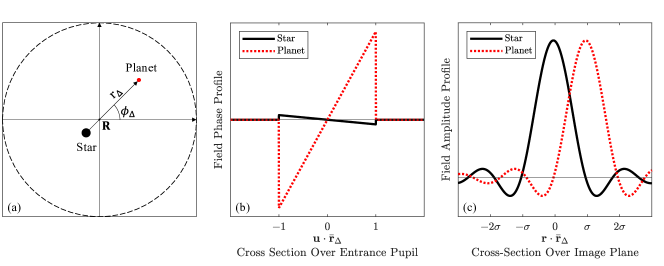
Figure 1: (a) Geometry of the star-planet model with the optical axis aligned to the center of intensity $\mathbf{R}$. The estimation parameters of the system are the polar components of the separation vector $\mathbf{r}_{\Delta}=(r_{\Delta},\phi_{\Delta})$. (b) Cross-section of the phase profiles over the pupil for the field generated by the star and planet independently. Note that the slight wavefront tilt in the field produced by the star arises from the system’s alignment to the center of intensity rather than to the star directly. However, in the high-contrast limit, the center of intensity asymptotically approaches the star position. (c) Cross-section of the amplitude profiles over the image plane for the fields produced by the star and planet independently. In the limit of high-contrast, the field produced by the star approaches the fundamental PSF mode since the optical axis nears coincidence with the star.

The parameters $b$ and $\mathbf{R}$ are taken to be known a priori such that localization amounts to estimating the unknown star-planet separation vector $\mathbf{r}_{\Delta}$. Simultaneous estimation of the separation vector, the centroid, and the relative brightness adds substantial complexity to the quantum information analysis which we defer to future studies. In the meantime, we point the curious reader to [13] for an interesting discussion on how the interdependence of these parameters manifests in the QFIM for the one-dimensional counterpart to our exoplanet localization problem.

2.3 Quantum Formulation of the Optical Field State

Formulating the quantum mechanical state of the optical field produced by our star-planet model allows us to calculate quantum information measures that establish the fundamental limits for exoplanet discovery tasks. Under the weak-source approximation for thermal sources (see Appendix B of [10]), the field in the pupil over a temporal coherence interval is either in the vacuum state with probability $1-\epsilon$ or occasionally in a single-photon excitation state with probability $\epsilon<<1$. Occupation numbers of more than one photon are assumed to be negligibly rare. The density operator describing the total mixed state of the field is therefore,

$$\hat{\rho}\equiv(1-\epsilon)\outerproduct{0}{0}+\epsilon\hat{\rho}_{1}+\mathcal{O}(\epsilon^{2})$$ (6)

where $\ket{0}$ is the vacuum state over all optical modes and,

$$\hat{\rho}_{1}\equiv(1-b)\outerproduct{\psi_{0}(\mathbf{r}_{s})}{\psi_{0}(\mathbf{r}_{s})}+b\outerproduct{\psi_{0}(\mathbf{r}_{e})}{\psi_{0}(\mathbf{r}_{e})}$$ (7)

is the single-photon mixed state encapsulating the possibility that the photon came from either the star or the planet. In particular, $\ket{\psi_{0}(\mathbf{r}_{s})}$ and $\ket{\psi_{0}(\mathbf{r}_{e})}$ are the single-photon pure states of the field for a photon emitted by the star and the planet respectively. These states can be expanded as a superposition of single-photon states in the position basis with amplitudes given by a shifted PSF,

$$\ket{\psi_{0}(\mathbf{s})}\equiv\int\psi_{0}(\mathbf{r}-\mathbf{s})\ket{\mathbf{r}}d^{2}r$$ (8)

The state $\ket{\mathbf{r}}=\hat{a}^{\dagger}(\mathbf{r})\ket{0}$ specifies the creation of single photon at position $\mathbf{r}$ on the image plane.

2.4 Quantum Measurement

Quantum information bounds are intrinsic to the quantum state, not on the measurement used to interrogate the state. Ultimately, it is the choice of measurement that determines whether an achievable quantum bound is reached. A measurement in quantum mechanics is formally defined by a positive operator-valued measure (POVM) - a set of positive semi-definite Hermitian operators $\{\hat{\Pi}_{\alpha}\}$ that sum to the identity operator on the Hilbert space $\sum_{\alpha}\hat{\Pi}_{\alpha}=\hat{I}$. Each operator has an associated outcome $\alpha$. The probability of observing outcome $\alpha$ when measuring a quantum state $\hat{\rho}$ is given by,

$$p_{\alpha}=\text{Tr}(\hat{\rho}\hat{\Pi}_{\alpha}).$$ (9)

Here we limit ourselves to von Neumann projective measurements - POVMs comprised of projectors $\hat{\Pi}_{\alpha}=\outerproduct{\pi_{\alpha}}{\pi_{\alpha}}$ that are orthogonal $\innerproduct{\pi_{\alpha}}{\pi_{\alpha^{\prime}}}=\delta_{\alpha\alpha^{\prime}}$. We find that such measurements suffice for saturating the quantum limits of exoplanet detection and localization. The term Direct Imaging corresponds to the POVM $\{\hat{\Pi}_{\mathbf{r}}=\outerproduct{\mathbf{r}}{\mathbf{r}}\}$ which represents the collection of single-photon states over the position modes. The term Spatial Mode Demultiplexing (SPADE), coined by [10], corresponds to the POVM $\{\hat{\Pi}_{\alpha}=\outerproduct{\psi_{\alpha}}{\psi_{\alpha}}\}$ which represents the collection of single-photon states in the orthonormal transverse spatial modes given by the functions $\psi_{\alpha}(\mathbf{r})$,

$$\ket{\psi_{\alpha}}=\int\psi_{\alpha}(\mathbf{r})\ket{\mathbf{r}}d^{2}r$$ (10)

Note that Direct Imaging is actually a special case of a SPADE measurement where the spatial modes are chosen to be Dirac delta functions $\psi_{\alpha}(\mathbf{r})=\delta(\mathbf{r}-\bm{\alpha})$. However, we typically reserve the term ’SPADE’ for a modal basis with non-trivial spatial variation. We also make note of a convenient mathematical property of hard apertures (i.e. systems with a binary pupil function) in the context of SPADE. Assume a mode basis $\{\tilde{\psi}_{\alpha}(\mathbf{u})\}$ has support over a binary pupil so that $\tilde{\psi}_{\alpha}(\mathbf{u})\tilde{\psi}_{0}(\mathbf{u})\propto\tilde{\psi}_{\alpha}(\mathbf{u})$. Then, the field generated by an off-axis point source at location $\mathbf{s}$ has basis expansion coefficients equal to,

$$\Gamma_{\alpha}(\mathbf{s})\equiv\innerproduct{\psi_{\alpha}}{\psi_{0}(\mathbf{s})}=\int\psi^{*}_{\alpha}(\mathbf{r})\psi_{0}(\mathbf{r}-\mathbf{s})d^{2}r=\frac{1}{\sqrt{\pi}}\psi^{*}_{\alpha}(\mathbf{s})$$ (11)

such that $\psi_{0}(\mathbf{r}-\mathbf{s})=\sum_{\alpha}\Gamma_{\alpha}(\mathbf{s})\psi_{\alpha}(\mathbf{r})$ (Appendix A). In other words, the basis expansion coefficients for the field state generated by a single off-axis source are proportional to the (complex conjugate) mode functions themselves evaluated at the source shift location. Hence the probability of detecting a photon in mode $\psi_{\alpha}$ for a given off-axis source is given by,

$$p_{\alpha}(\mathbf{s})=|\Gamma_{\alpha}(\mathbf{s})|^{2}=\frac{1}{\pi}|\psi^{*}_{\alpha}(\mathbf{s})|^{2}$$ (12)

a useful fact that we employ in later derivations and numerical simulations.

2.5 Quantum Formulation of the Coronagraph Operator

A coronagraph is a passive linear system can be mathematically modelled as a mode-selective optical attenuator [20, 9]. We formalize this description quantum mechanically by an operator,

$$\hat{C}=\sum_{k}\tau_{k}\outerproduct{\chi_{k}}{\chi_{k}}$$ (13)

that acts on the subspace of single-photon states (Appendix E). Here $\chi_{k}(\mathbf{r})$ are the eigenmodes of the propagator for particular coronagraph and $\tau_{k}$ are complex transmission coefficients (eigenvalues) of each eigenmode. Critically, coronagraphs are mathematically defined and distinguished by their eigenmodes and associated transmission coefficients. The eigenmodes form a complete orthonormal basis such that $\innerproduct{\chi_{k}}{\chi_{k^{\prime}}}=\delta_{kk^{\prime}}$. By definition, the coronagraph operator satisfies the eigenequation $\hat{C}\ket{\chi_{k}}=\tau_{k}\ket{\chi_{k}}$, such that propagating the single-photon state $\ket{\chi_{k}}$ through the coronagraph delivers the same state of the optical field up to a complex factor. We emphasize that for any coronagraph which achieves complete nulling of an on-axis source, the fundamental mode of the telescope necessarily lives in the null space of the coronagraph operator. That is, $\chi_{0}(\mathbf{r})\equiv\psi_{0}(\mathbf{r})$ is an eigenmode of the coronagraph with transmission coefficient $\tau_{0}=0$ such that $\hat{C}\ket{\psi_{0}}=0$. In general, propagating any single-photon mixed state through a coronagraph results in the state,

$$\hat{\rho}^{\prime}_{1}=\hat{C}\hat{\rho}_{1}\hat{C}^{\dagger}$$ (14)

Clearly, the output state $\hat{\rho}^{\prime}_{1}$ is no longer unit trace due to light loss from attenuation through the coronagraph,

$$\text{Tr}(\hat{\rho}^{\prime})=\sum_{k}|\tau_{k}|^{2}\matrixelement{\chi_{k}}{\hat{\rho}}{\chi_{k}}$$

As we later show, this fact demands some modification of the classical information measures considered in our work to sensibly handle non-normalized states.

3 Exoplanet Detection and the Quantum Chernoff Bound

Exoplanet detection amounts to performing a binary hypothesis test between two possible quantum states of the incident optical field. The result of this test declares whether an exoplanet is absent or present around a candidate host star. If the exoplanet is absent, then the state is given by the single-photon excitation of the PSF mode $\hat{\rho}_{0}=\outerproduct{\psi_{0}}{\psi_{0}}$ because the optical system is aligned to the star. If the exoplanet is present, then the state is given by $\hat{\rho}_{1}$ defined in Eq. 7. The total probability of error for a detection problem is given by the sum of false-positive probability (type I error) and false-negative probability (type II error). Supposing we measure $N$ identical copies of an unknown single-photon field state (either $\hat{\rho}_{0}$ or $\hat{\rho}_{1}$), the minimum probability of error for discriminating whether the field state is $\hat{\rho}_{0}$ or $\hat{\rho}_{1}$ asymptotically follows the Quantum Chernoff Bound (QCB) in large $N$,

$$P_{e,min}\sim e^{-N\xi_{Q}}$$ (15)

where the Quantum Chernoff Exponent (QCE) is given by [21],

$$\xi_{Q}\equiv-\log(\min_{0\leq s\leq 1}\text{Tr}(\hat{\rho}_{0}^{s}\hat{\rho}_{1}^{1-s}))$$ (16)

Incorporating the relative probability $\epsilon$ of single-photon states over the vacuum into the error probability simply involves replacing $N$ with $\epsilon N$. We find that the QCE for discriminating the absence or presence of an exoplanet (Appendix B) is given by ,

$$\xi_{Q}(\mathbf{r}_{\Delta})=-\log[(1-b)|\Gamma_{0}(-b\mathbf{r}_{\Delta})|^{2}+b|\Gamma_{0}((1-b)\mathbf{r}_{\Delta})|^{2}\bigg{]}$$ (17)

In the high-contrast regime where $b\rightarrow 0$, the QCE tends towards,

$$\boxed{\xi_{Q}(\mathbf{r}_{\Delta})\xrightarrow[]{b<<1}b\bigg{[}1-|\Gamma_{0}(\mathbf{r}_{\Delta})|^{2}\bigg{]}}$$ (18)

Telescope Diameter	$6.5\,\text{m}$ (Next-Gen Space Telescope)
Center Wavelength	$1290$ nm
Bandwidth	$13$ nm ($\sim 1\%$)
Star Visual Magnitude (VM)	$5.357$ (Proxima Centauri J-Band)
Reference Flux (VM=0)	$1589\times 10^{-26}\,\text{W}\text{m}^{-2}\text{Hz}^{-1}$
Photon Flux	$6\times 10^{7}$ Photons $s^{-1}$

Table 1: Reference values for calculating exposure times necessary to reach detection and localization performance isocontours in Fig.s 2b and 3b respectively.

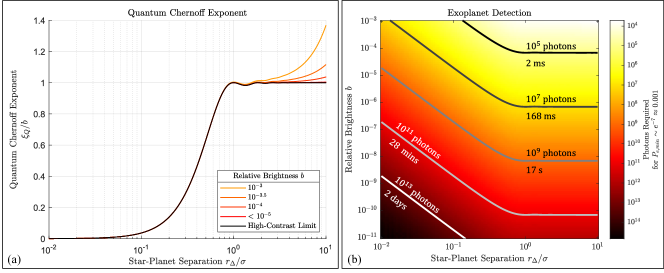
Figure 2: (a) The Quantum Chernoff Exponent (QCE) as a function of the star-planet separation. The QCE has been normalized by the relative brightness $b$ to show convergence towards the high-contrast limit derived in Eq. 18. (b) A map of the photon requirement for reaching an exoplanet detection confidence of $99.9\%$ using a quantum-optimal system that saturates the Quantum Chernoff Bound. The isocontours represent boundaries of the problem space above which declaring the presence or absence of an exoplanet can be made with $\geq 99.9\%$ confidence. To provide a practical sense of the timescales required to achieve the confidence limits, the quoted photon counts are converted to integration times for a given telescope prescription, stellar magnitude, and waveband defined in Table 1.

In this limit, the QCE enjoys a simple interpretation - it approaches the probability that a photon coming from the exoplanet arrives ’outside’ of the fundamental mode (i.e. in the orthogonal complement space of the fundamental mode). The high-contrast QCE suggests that separating photons in the fundamental mode from photons in its orthogonal complement constitutes an optimal strategy for exoplanet detection (proof in [22]). A positive exoplanet detection is declared if any photons are registered in the orthogonal complement space within the integration period.

Fig. 2(a) shows the QCE as a function of the star-planet separation converging to the high-contrast limit,

$$\xi_{Q}(r_{\Delta})\xrightarrow[]{b<<1}b\bigg{[}1-\bigg{(}\frac{J_{1}(2\pi r_{\Delta})}{\pi r_{\Delta}}\bigg{)}^{2}\bigg{]}$$ (19)

for a telescope with a circular pupil. We draw attention to certain values of the high-contrast QCE at different star-planet separations. As one would expect, the QCE disappears at zero separation since distinguishing between one on-axis source and two overlapping on-axis sources is impossible. The QCE is maximal wherever the star-planet separation corresponds to a node (zero) of the PSF. This is because no light from a point source situated at a node couples into the fundamental mode (a consequence of Eq. 11). Necessarily, the light must couple to higher-order modes if energy is to be conserved. Therefore, exoplanets which happen to reside near a node of the PSF may be detected with fewer photon resources. The exponential tails of the QCE observed for intermediate contrasts (e.g. $10^{-3}$ to $10^{-4}$) and large star-planet separations $r_{\Delta}>1$ result from starlight coupling to higher-order modes when the system aligned to the center of intensity. At these moderate contrasts any photon detected outside the PSF mode, whether it be from the star or the exoplanet, is an indication that an exoplanet is present. Fig. 2(b) shows detection working regions for different pairings of relative brightness and star-planet separations.

Formally, a particular measurement defined by POVM $\{\hat{\Pi}_{\alpha}\}$ is said to achieve/saturate the QCB if the Classical Chernoff Exponent (CCE) equals the QCE. The CCE is given by,

$$\xi_{C}\equiv-\log(\min_{0\leq t\leq 1}\sum_{\alpha}p_{0\alpha}^{t}p_{1\alpha}^{1-t})\leq\xi_{Q}$$ (20)

where $p_{0\alpha}=\text{Tr}(\hat{\rho}_{0}\hat{\Pi}_{\alpha})$ and $p_{1\alpha}=\text{Tr}(\hat{\rho}_{1}\hat{\Pi}_{\alpha})$. The sum is promoted to an integral if the outcomes of the measurement are continuous. A sensible rendition of the CCE applicable to coronagraphy is described in Appendix I.

4 Exoplanet Localization and the Quantum Fisher Information Matrix

To localize an exoplanet we consider applying an unbiased estimator over outcomes of measurements on the quantum field state. In general, the covariance matrix of an unbiased estimator $\check{\bm{\theta}}$ of the parameters $\bm{\theta}=[\theta_{1},\ldots,\theta_{n}]$ characterizing a quantum state $\hat{\rho}(\bm{\theta})$ is lower bounded by the Quantum Cramer-Rao Bound (QCRB)

$$\text{Cov}[\check{\bm{\theta}}]\geq\bm{\Sigma}_{Q}=\frac{1}{N}\bm{\mathcal{K}}^{-1}$$ (21)

where $\bm{\mathcal{K}}$ is the Quantum Fisher Information Matrix (QFIM), $N$ is the number of copies of $\hat{\rho}(\bm{\theta})$ measured, and the inequality indicates that $\text{Cov}[\check{\bm{\theta}}]-\bm{\Sigma}_{Q}\geq 0$ is a positive semi-definite matrix. Thus, given a finite number of copies of the state, any set of parameters (or linear combinations thereof) can be estimated up to a minimum uncertainty determined by the laws of physics. The entries of the QFIM are given by,

$$\mathcal{K}_{ij}=\frac{1}{2}\text{Tr}(\hat{\rho}\{\hat{L}_{i},\hat{L}_{j}\})$$ (22)

where $\{\cdot,\cdot\}$ represents the anti-commutator and $\hat{L}_{i}$ is the symmetric logarithmic derivative (SLD) for the parameter $\theta_{i}$ that solves the implicit equation,

$$\partial_{\theta_{i}}\hat{\rho}=\frac{1}{2}(\hat{\rho}\hat{L}_{i}+\hat{L}_{i}\hat{\rho}).$$ (23)

where $\partial_{\theta}=\frac{\partial}{\partial\theta}$ compactly denotes the partial derivative. A measurement defined by POVM $\{\hat{\Pi}_{\alpha}\}$ is said to be quantum-optimal if the Classical Fisher Information Matrix (CFIM) is equal to the QFIM. The CFIM for a set of parameters $\bm{\theta}$ is given by,

$$\mathcal{I}_{ij}=\sum_{\alpha}\mathcal{I}_{\alpha,ij}=\sum_{\alpha}p_{\alpha}\big{(}\partial_{\theta_{i}}\log p_{\alpha}\big{)}\big{(}\partial_{\theta_{j}}\log p_{\alpha}\big{)}$$ (24)

where $\mathcal{I}_{\alpha,ij}$ is the CFI contribution of the POVM element $\hat{\Pi}_{\alpha}$ and the sum over $\alpha$ is promoted to an integral if the measurement outcome probability distribution $p_{\alpha}$ is continuous. Applying this formalism to the exoplanet localization task, we use results from [23] to determine the QFI matrix for any optical system with a real $\tilde{\psi}_{0}(\mathbf{u})\in\mathbb{R}$ and inversion-symmetric pupil function $\tilde{\psi}_{0}(-\mathbf{u})=\tilde{\psi}_{0}(\mathbf{u})$ which give rise to a purely real PSF $\psi_{0}(\mathbf{r})\in\mathbb{R}$. When aligned to the center of intensity, the QFIM of the star-planet separation $\mathbf{r}_{\Delta}$ is given by (Appendix C),

$$\bm{\mathcal{K}}=\frac{1}{4}(1-\kappa^{2})\bigg{[}\bm{\mathcal{K}}_{1}-\kappa^{2}\bm{\mathcal{I}}_{0}\bigg{]}$$ (25)

where the constant $\kappa\equiv(1-b)-b$ is the difference in relative brightness and the matrices $\bm{\mathcal{K}}_{1}$ and $\bm{\mathcal{I}}_{0}$ are,

$$\mathcal{K}_{1,ij} =4\langle\partial_{\theta_{i}}(2\pi\mathbf{u}\cdot\mathbf{r}_{\Delta})\partial_{\theta_{j}}(2\pi\mathbf{u}\cdot\mathbf{r}_{\Delta})\rangle$$ (26a)

$$\mathcal{I}_{0,ij} =4\big{(}\partial_{\theta_{i}}\Gamma_{0}(\mathbf{r}_{\Delta})\big{)}\big{(}\partial_{\theta_{j}}\Gamma_{0}(\mathbf{r}_{\Delta})\big{)}$$ (26b)

with $\langle\cdot\rangle$ indicating an average over the pupil function

$$\langle\tilde{f}(\mathbf{u})\rangle\equiv\int|\tilde{\psi}_{0}(\mathbf{u})|^{2}\tilde{f}(\mathbf{u})d^{2}u$$ (27)

Critically, $\bm{\mathcal{K}}_{1}$ is the QFIM associated with localizing a single point source and $\bm{\mathcal{I}}_{0}$ is the CFIM contribution of the fundamental mode. In the high-contrast limit where $b\rightarrow 0$, we keep terms of linear order in $b$ to arrive at the approximation,

$$\boxed{\bm{\mathcal{K}}\xrightarrow[]{b<<1}b\bigg{[}\bm{\mathcal{K}}_{1}-\bm{\mathcal{I}}_{0}\bigg{]}}$$ (28)

In this form, the QFIM lends itself to an intuitive interpretation - it is the information associated with localizing a single point source if all information in the fundamental mode were unavailable. This interpretation reinforces a long-held intuition within the astronomy community that the fundamental mode is too noisy to be of value in exoplanet searches since it is dominated by photons from the star. The asymptotic QFIM indicates that the fundamental mode can be rejected without incurring information losses about the exoplanet that were otherwise recoverable. In hindsight, it is remarkable that high-contrast QCE of Eq. 18 and the high-contrast QFIM of Eq. 28 allude to identical messages despite being information-theoretic measures for two entirely different tasks. Namely, that the fundamental mode of the imaging system can readily be dispensed with in the high-contrast regime. This theoretical insight is highly suggestive of optimal measurement schemes which we explore in the next section.

For a circular pupil, the QFIM for polar parameterization of the star-planet separation vector $\theta_{i}\in\{r_{\Delta},\phi_{\Delta}\}$ is given by,

$$\bm{\mathcal{K}}^{(r\phi)}=(1-\kappa^{2})\pi^{2}\Bigg{(}\begin{bmatrix}1&0\\ 0&r^{2}_{\Delta}\end{bmatrix}-\kappa^{2}\bigg{(}\frac{2\,J_{2}(2\pi r_{\Delta})}{\pi r_{\Delta}}\bigg{)}^{2}\begin{bmatrix}1&0\\ 0&0\end{bmatrix}\Bigg{)}.$$ (29)

The QFI matrix conveniently becomes diagonal due to the rotational symmetry of the pupil. Note that when the sources have equal brightness ($b=0.5$), the second term vanishes. This recovers the well-known result that the QFI of the separation between two balanced point sources remains constant, irrespective of the separation itself [11]. Otherwise, for unequal brightness ($b\neq 0.5$) the second term persists and the QFI for the star-planet separation acquires a dependence on $r_{\Delta}$. Meanwhile, the QFI for the angular orientation of the sources grows quadratically in $r_{\Delta}$, matching a general intuition that angular sensitivity scales with the length of the lever arm. In the high-contrast limit the QFIM for a circular pupil is well-approximated by,

$$\bm{\mathcal{K}}^{(r\phi)}\xrightarrow[]{b<<1}4\pi^{2}\,b\Bigg{(}\begin{bmatrix}1&0\\ 0&r^{2}_{\Delta}\end{bmatrix}-\bigg{(}\frac{2\,J_{2}(2\pi r_{\Delta})}{\pi r_{\Delta}}\bigg{)}^{2}\begin{bmatrix}1&0\\ 0&0\end{bmatrix}\Bigg{)}$$ (30)

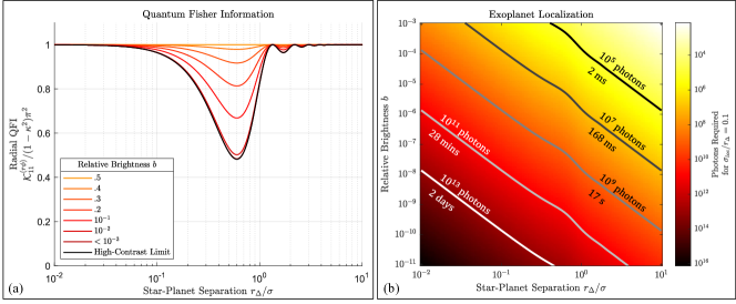
Figure 3: (a) The Quantum Fisher Information (QFI) of the radial parameter $r_{\Delta}$ for different relative brightness values. The QFI has been normalized with respect to the common contrast-dependent factor $(1-\kappa^{2})\pi^{2}$ in Eq. 29 to show the QFI curves approaching the high-contrast limit expressed in Eq. 30. The prominent dip in the QFI corresponds to where the classical Fisher information contribution of the PSF mode is maximal. Since the fundamental mode is dominated by photons from the star, its information is suppressed by a factor of $b$ compared to higher-order modes. (b) A map of the photon requirement for achieving a relative localization error of $\sigma_{loc}/r_{\Delta}=0.1$. Each isocontour demarcates regions of the problem space above which the relative localization imprecision is $\sigma_{loc}/r_{\Delta}<0.1$. To provide a practical sense of the timescales required to achieve the imprecision limits, the quoted photon counts are converted to integration times for a given telescope prescription, stellar magnitude, and waveband defined in Table 1.

Fig. 3(a) shows the convergence of the radial parameter QFI towards the high-contrast limit. To convert the QFIM to a practical measure of the localization precision we consider summing the QCRB variances of the estimation parameters. In polar coordinates, this imprecision is characterized by an uncertainty area patch,

$$\sigma^{2}_{loc}\equiv\sigma_{r_{\Delta}}^{2}+(r_{\Delta}\sigma_{\phi_{\Delta}})^{2}=\frac{1}{N}\bigg{[}\frac{1}{\mathcal{K}^{(r\phi)}_{11}}+\frac{r_{\Delta}^{2}}{\mathcal{K}^{(r\phi)}_{22}}\bigg{]}$$ (31)

A practically valuable metric to consider is the number of photons needed to localize the exoplanet up to a fraction of the star-planet separation $\frac{\sigma_{loc}}{r_{\Delta}}$ (i.e. relative error). Fig. 3(b) shows an isocontour map indicating the number of photons required to reach 10% relative localization error over a range of star-planet separations and contrasts.

5 Quantum-Optimal Systems for Exoplanet Detection and Localization

In this section we describe two quantum-optimal systems: SPADE and the Perfect Coronagraph (PC). We prove that both systems saturate the quantum limits of exoplanet detection and localization in the high-contrast regime (Appendix G for SPADE and Appendix H for PC). Fig. 4 shows possible implementations of either system using an abstract spatial mode-sorting element. Similar implementations of mode-sorter-based coronagraphs have been proposed that employ photonic lanterns [24] and multi-plane light converters [25].

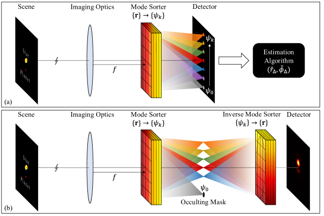
Figure 4: (a) PSF-matched SPADE: A system that decomposes the incident optical field into a set of orthonormal transverse spatial modes and counts the number of photons in each mode channel. In the implementation shown, the field incident on the focal plane is transformed from a position basis $\{\mathbf{r}\}$ into PSF-matched mode basis $\{\psi_{k}(\mathbf{r})\}$ by directing each spatial mode to disjoint diffraction-limited spots on a detector. (b) Perfect Coronagraph (PC): A direct imaging system that exclusively eliminates the fundamental mode of the telescope prior to detection. Higher order modes are left unaffected. In the implementation shown, the field incident on the focal plane is sorted into a PSF-matched mode basis. The fundamental mode is occluded at the sorting plane. Residual light in the orthogonal modes propagates freely to an inverse mode sorter that reverts the light back into the position basis before measuring an intensity distribution at a detector.

5.1 PSF-Matched SPADE

For a SPADE system light incident on the image plane is sorted into a basis of orthogonal transverse spatial modes as shown in Fig. 4(a). Critically, in a PSF-matched SPADE basis the zeroth order mode of the basis is the fundamental mode of the imaging system. A complete measurement consists of counting the total number of photons arriving in each mode channel over a given integration time. A positive exoplanet detection is heralded if a photon arrives in any mode other than the PSF mode. An exoplanet is localized by running an estimator (e.g. maximum likelihood) on the complete measurement outcome. In principle, an image of the scene itself can be retroactively reconstructed if one measures the amplitude and phase of each mode channel instead of measuring their intensity. While photon counting suffices for estimating the location of a single exoplanet, it may be advantageous to reconstruct the field from amplitude and phase measurements if the number of exoplanets is unknown.

In this work, we consider a particular SPADE system that sorts the Zernike modes defined in Appendix F. These modes constitute a PSF-matched basis for imaging systems with a circular pupil. In Fig. 5 we investigate how the distribution of Fisher information over the mode channels varies with respect to the star-planet separation. We see that the fundamental mode contains virtually zero information about the star-planet separation. Instead, the information diffuses into higher-order modes as the star-planet separation increases. For sub-diffraction separations, the information is highly concentrated in the tip-tilt modes. The lack of information in the fundamental mode is mathematically justified by the asymptotic scaling behavior of a PSF-matched mode basis in the high-contrast regime. In Appendix G we show that the CFI contribution of the fundamental mode scales as $\mathcal{I}^{(r\phi)}_{0,ij}\propto b^{2}$ while the CFI contribution of higher-order modes scales as $\mathcal{I}^{(r\phi)}_{k>0,ij}\propto b$.

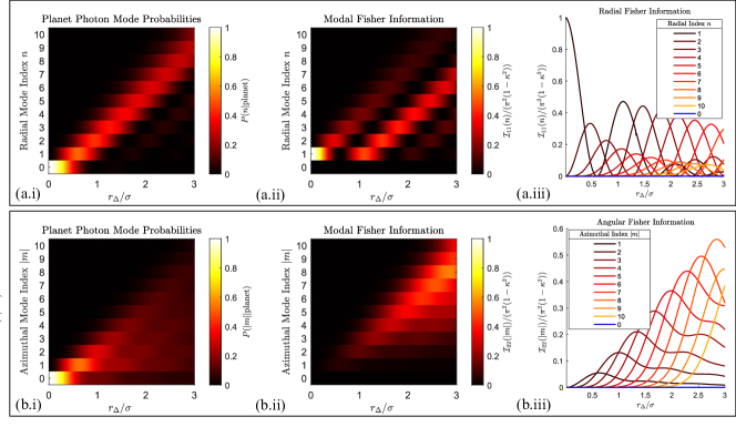
Figure 5: Decomposition of the Classical Fisher Information per Zernike mode over different star-planet separations. (a) Shows the information of the radial parameter $r_{\Delta}$ decomposed by radial mode index $n$. (b) Shows the information of the angular parameter $\phi_{\Delta}$ decomposed by azimuthal mode index $|m|$. The relative brightness was set to $b=10^{-9}$ and the orientation angle of the star-planet system was set to $\phi_{\Delta}=\pi/4$ radians offset from the x-axis. The left-most sub panels show the evolution of the modal coupling probabilities for photons emitted by the exoplanet as a function of the star-planet separation. We see that the coupling probabilities spread to higher-order modes as the star-planet separation increases. The fundamental mode (index $0$) carries virtually no information about the separation parameters, yet starlight overwhelmingly couples into this mode in the high-contrast regime.

5.2 Perfect Coronagraph

The PC is characterized by a direct imaging system that exclusively removes the fundamental mode from the field prior to detection without affecting higher-order modes. It is described compactly by the coronagraph operator,

$$\hat{C}=\hat{\mathds{1}}-\outerproduct{\psi_{0}}{\psi_{0}}$$ (32)

where $\hat{\mathds{1}}$ is the identity. Fig. 4(b) depicts one possible implementation of the PC using mode sorting elements. Like the SPADE system, light is sorted into a set of PSF-matched modes. However, rather than count photons in each mode channel, the PSF mode channel is rejected with a mask while all other modes are left to propagate freely past the sorting plane. Subsequently, an inverse mode sorter is applied to convert the field in the sorting plane back into an image. A positive exoplanet detection is heralded if a photon arrives at the detector plane at all. An exoplanet is localized by running an estimator on the irradiance distribution measured at the detector. Unlike SPADE measurements, direct imaging bears some perceptual resemblance to the scene itself. With the star eliminated the image may be used to infer the presence of multiple exoplanets.

6 High-Performance Coronagraphs

In this section, we define two state-of-the-art coronagraphs: the Phase-Induced Amplitude Apodization Complex Mask Coronagraph (PIAACMC)[26] and the Vortex Coronagraph (VC) [27]. Both the PIAACMC and VC theoretically achieve complete rejection of an on-axis point source. Thus, the fundamental mode lives in the null space of their respective coronagraph operators. These coronagraphs modulate the phase and amplitude of different optical modes at the focal plane using a (generally complex) transmission mask. The masks are designed to offer on-axis nulling of the star by diffracting light outside the clear aperture support of a downstream Lyot stop. We provide a brief overview of each of these coronagraphs. For a more comprehensive explanation of advanced Lyot-style coronagraphs we refer the interested reader to [8].

Figure 6: Two state-of-the-art direct imaging coronagraphs that achieve complete rejection of an on-axis point source.(a) Phase-induced Amplitude Apodization Complex Mask Coronagraph (PIAACMC): Employs aspheric optics to induce a lossless prolate spheroidal apodization. The complex phase mask causes the apodized fundamental mode to destructively interfere and cancel in the clear aperture of the Lyot stop.(b) Vortex Coronagraph (VC): A direct imaging coronagraph that diffracts the fundamental mode outside the Lyot stop using a (charge 2) vortex phase mask with integer topological charge.

6.1 Phase-Induced Amplitude Apodization Complex Mask Coronagraph

For an appropriate choice of pupil apodization in combination with a $\pi$-phase mask placed at the focal plane of the objective (i.e. Roddier and Roddier Coronagraph [28]), complete extinction of an on-axis star can be achieved. The appropriate spatial profile of the apodization function is a member of the prolate spheroids specific to the geometry of the pupil [29, 30, 31]. These are eigenfunctions of the finite Fourier transform over the aperture support. The PIAACMC employs aspheric optics to redistribute the light over the pupil and achieve the required spatial apodization for complete star extinction [26]. The use of refractive elements to induce apodization as opposed to a spatial transmission mask preserves light throughput past the pupil. Phase modulating the apodized fundamental mode at the focal plane with a $\pi$-phase mask causes the field to destructively interfere with itself such that the amplitude is zero within the clear aperture area of a downstream Lyot Stop. For off-axis sources, self-interference induced by the phase mask does not cancel the field and light passes through the Lyot stop. Any distortion generated by the first set of aspheric surfaces is compensated by a set of identical but inverted aspheric surfaces before imaging the field onto a detector.

6.2 Vortex Coronagraph

The vortex coronagraph first proposed by [27] introduces a vortex phase plate with integer topological charge at the focal plane of the objective. This element introduces a helical phase modulation of the field. The phase modulation diffracts light in the fundamental mode outside the clear aperture area of a downstream Lyot stop. Off-axis sources will instead acquire a near-constant phase over the bulk of their field amplitude and pass through the system relatively unaltered. Vortex coronagraphs and vortex fiber nullers have been the subject of several sub-diffraction exoplanet imaging demonstrations in recent years [32, 33, 34, 35, 36]. For all figures and comparative performance analysis presented herein, we consider a charge-2 vortex.

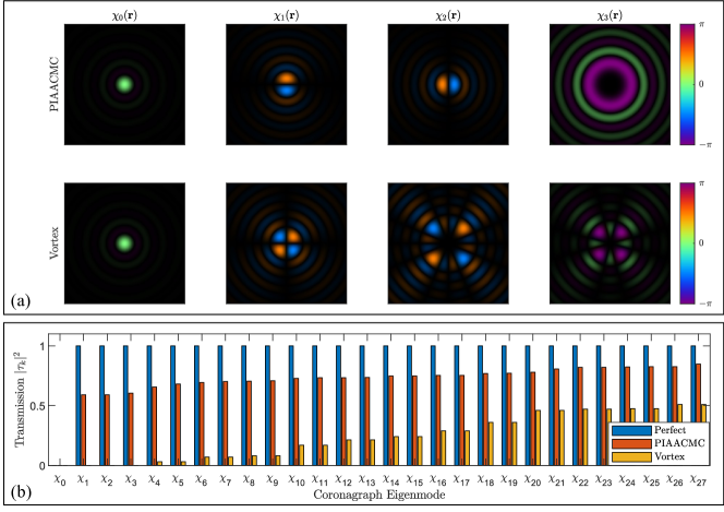
Figure 7: (a) Eigenmodes of the PIAACMC and Vortex coronagraph shown in ascending order of transmission (left to right). Each coronagraph has a unique set of eigenmodes specific to its propagator. Note that the fundamental mode (left panel) is a common eigenmode of both systems and exhibits the lowest transmission. (b) Magnitude squared of the complex transmission coefficients for the first 28 eigenmodes of the Perfect, PIAACMC, and Vortex coronagraph. The Perfect coronagraph nulls only the fundamental mode and has unit transmission for all higher-order eigenmodes. Meanwhile, the PIAACMC and Vortex coronagraph exhibit varying degrees of attenuation for higher-order eigenmodes. In general as the mode order increases the transmission increases quickly for the PIAACMC but slowly for the Vortex.

7 Results

7.1 Exoplanet Detection Comparison

In Fig. 8(a) we compare the CCE of each coronagraph against the QCE limit for three different contrasts. The SPADE and PC saturate the QCE at all contrasts due to complete rejection of hypothesis $\hat{\rho}_{0}$ and minimal attenuation of hypothesis $\hat{\rho}_{1}$. The PIAACMC and the VC demonstrate sub-optimal exoplanet detection performance due to attenuation of modes beyond the fundamental which are active under hypothesis $\hat{\rho}_{1}$. The quantum-optimal SPADE and PC systems achieve $\sim 1.6\times$ and $\sim 2\times$ maximum enhancement in the Chernoff exponent over PIAACMC and VC respectively. In practice, quantum-optimal systems are therefore projected to reach the same level of exoplanet detection confidence as the PIAACMCM and VC in about half the integration time for exoplanets located below the diffraction limit. Table 2 shows the integration time required with each coronagraph to reach progressively lower probabilities of detection error for an example star-planet system and telescope prescription.

In Fig. 7 we show four eigenmodes of the PIAACMC and the VC with lowest transmission factors $|\tau_{k}|^{2}$. We see that the The fundamental mode lies in the null space of both coronagraphs. The next most attenuated eigenmodes for both high-performance coronagraphs are linear combinations of the tip-tilt modes. These modes are active for small off-axis displacements of the exoplanet. Thus, the superior performance of the PIAACMCM compared to the VC at small star-planet separations stems from its comparatively higher transmission of tip-tilt modes.

In Appendix I we show that the high-contrast CCE is the throughput scaled by relative brightness of the exoplanet,

$${}_{C}\xrightarrow[]{b<<1}b \text{Tr}(\hat{C}\outerproduct{\psi_{0}(\mathbf{r}_{\Delta})}{\psi_{0}(\mathbf{r}_{\Delta})}\hat{C}^{\dagger})$$

$$=b \sum_{k}|\tau_{k}|^{2}|\innerproduct{\chi_{k}}{\psi_{0}(\mathbf{r}_{\Delta})}|^{2}$$ (33)

for any direct imaging coronagraph that contains $\ket{\psi_{0}}$ in the null space of its coronagraph operator $\hat{C}$. In these systems, the probability making a detection error arises solely from false-negative events. False-positive events are mathematically impossible. The probability of error is driven down by the likelihood of true-positive events alone. Hence, the CCE is the probability that a photon from the exoplanet avoids being rejected by the coronagraph and arrives successfully at the detector (i.e. throughput).

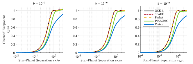
Figure 8: Comparisons between the classical Chernoff exponent (CCE) as a function of star-planet separation different coronagraph systems. All curves are normalized by the star-planet contrast corresponding to each panel. SPADE and the Perfect coronagraph are quantum-optimal exoplanet detection methods as they saturate the quantum Chernoff exponent (QCE). While the PIAACMC and Vortex coronagraph eliminate all on-axis starlight, they also excessively attenuate exoplanet light coupling to higher-order modes leading to sub-optimal exoplanet detection capabilities.

Coronagraph	$P_{e}=10^{-1}$	$P_{e}=10^{-2}$	$P_{e}=10^{-3}$	$P_{e}=10^{-4}$
Perfect/SPADE	1,073	2,146	3,220	4,293
PIAACMC	1,663	3,326	4,990	6,653
Vortex	2,167	4,334	6,501	8,668

Table 2: Integration times (in seconds) required to reach different probability of errors for exoplanet detection. For this example, an exoplanet is located around a star with $r_{\Delta}/\sigma=0.1$ and $b=10^{-9}$. The star photon flux and telescope specifications used are given in Table 1.

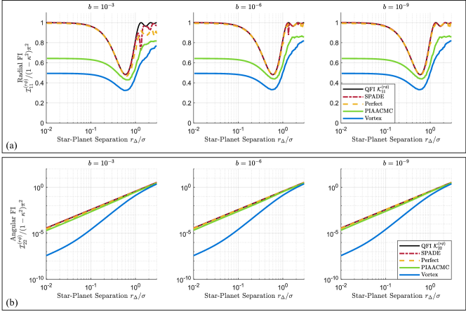
Figure 9: A comparison of the Classical Fisher Information (CFI) of (a) the star-planet separation and (b) the angular orientation achieved with different coronagraphs for three different contrasts $b=10^{-3},10^{-6},10^{-9}$. The upper bound of the CFI is given by the Quantum Fisher Information (QFI) shown in black which we see is saturated by the Perfect coronagraph and the SPADE coronagraph (truncated at a maximum radial mode order of $\max{n}=500$) in the limit of high contrast. The PIAACMC and the Vortex Coronagraph are sub-optimal particularly in the deep sub-Rayleigh regime $r_{\Delta}/\sigma<0.1$.

Coronagraph	$\frac{\sigma_{loc}}{r_{\Delta}}=1$	$\frac{\sigma_{loc}}{r_{\Delta}}=\frac{1}{2}$	$\frac{\sigma_{loc}}{r_{\Delta}}=\frac{1}{10}$	$\frac{\sigma_{loc}}{r_{\Delta}}=\frac{1}{100}$
Perfect/SPADE	6	25	626	62,596
PIAACMC	9	37	927	92,749
Vortex	33	134	3,350	335,000

Table 3: Integration times (in seconds) required to reach different relative localization errors for an exoplanet around a star with $r_{\Delta}/\sigma=0.1$ and $b=10^{-9}$. The star photon flux and telescope specifications used are given in Table 1.

7.2 Exoplanet Localization Comparison

In Fig. 9 we directly compare the radial and angular CFI of SPADE, PC, PIAACMC and VC against the QFI at three different contrast levels. The CFI curves for SPADE and PC fully saturate the QFI at sub-diffraction star-planet separations for all contrasts shown. In the super-diffraction regime they progressively approach the QFI at higher contrasts. In all separation and contrast regimes, the SPADE and PC information curves are strictly greater than those of the PIAACMC and VC. For the radial parameter $r_{\Delta}$, Fig. 9(a) indicates that SPADE and PC are roughly $2\times$ as information-efficient as PIAACMC and VC in the deeply sub-diffraction regime $(r_{\Delta}\lesssim\sigma/10)$ for all contrasts shown. This performance difference occurs due to lower-order mode attenuation in the PIAACMC and VC as shown in 7(b). When the star and exoplanet are well-separated $(r_{\Delta}\gtrsim 2\sigma)$, then the CFI for all systems converge as light begins coupling to higher-order modes that exhibit higher transmission.

For the angular parameter $\phi_{\Delta}$, Fig. 9(b) shows that both SPADE and PC saturate the QFI limit at all contrasts. In the sub-diffraction regime, SPADE and the PC are approximately $2\times$ and $100\times$ more information efficient than the PIAACMC and VC respectively. The drastic sub-optimality of the VC at small star-planet separations can be deduced by inspecting the actual images that each coronagraphs create as shown in Fig 10. The images after the Perfect coronagraph show the double-lobed structure that is expected from the tip-tilt modes after subtraction of the fundamental mode. The modeled PIAACMC has a nearly visually indistinguishable structure with only a lower transmission. This means that the PIAACMC nulls the fundamental mode and small amounts of the tip-tilt modes. The Vortex Coronagraph however, creates doughnut like structures even near the diffraction-limit which increases uncertainty about the angular orientation of the star-planet axis.

Practically, the relative difference in Fisher information between each system dictates the difference in the exposure time each require to achieve a particular exoplanet localization precision. Table 3 compares these exposure times between each coronagraph for an example sub-diffraction star-planet system and telescope prescription. In general, we see that SPADE and PC offer salient performance improvements over PIAACMC and VC primarily in the sub-diffraction regime. To illustrate the prospective value of quantum-optimal systems Fig. 11(b) depicts Monte-Carlo simulations of sub-diffraction exoplanet localization using SPADE measurements.

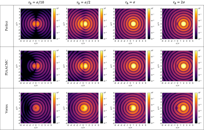
Figure 10: Simulated measurements for direct imaging coronagraphs pointed at the center of intensity of a star-planet system with $b=10^{-9}$. Each column corresponds to a different star-planet separation along an axis oriented at angle $\phi_{\Delta}=0$. In the sub-Rayleigh regime $r_{\Delta}<\sigma$ the detected intensity does not bear perceptual resemblance to a diffraction-limited planet spot. The two-lobe structure visible in column 1 for the PC and PIAACMCM emerges due to dominant coupling to the tilt modes at small separations. Note that the vortex coronagraph does not exhibit a two-lobe structure as the tilt modes are highly attenuated. Consequently, the sensitivity of the Vortex coronagraph to radial separation $r_{\Delta}$ and the angular orientation of the star-planet system suffers as shown by the sub-optimal CFI curves of Fig. 9.

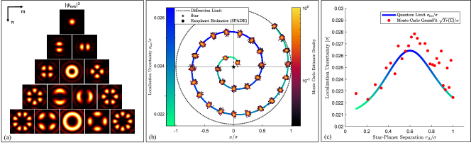
Figure 11: (a) The squared magnitude of the first 15 Fourier-Zernike modes. (b) Monte-Carlo simulations showing localization of an exoplanet at various sub-Rayleigh distances from the star location using maximum likelihood estimation on SPADE measurements in the Fourier Zernike basis, truncated to maximum radial order $\text{max}(n)=10$. For each exoplanet location, $500$ measurement and estimation trials were simulated. The brightness contrast was set to $b=10^{-9}$ and the mean photon count per measurement was taken to be $300\times 10^{9}$ such that, on average, $\sim 300$ photons from the exoplanet were collected per measurement. We have chosen exoplanet locations spaced equally over a spiral to illustrate variations in uncertainty that may depend on radial or angular position in the field of view. (c) Quantified variation in the size of the uncertainty patch for each cluster of exoplanet estimates. For each cluster, we fit a 2D Gaussian distribution and compute an uncertainty patch from the covariance matrix. We see that the size of the uncertainty patches roughly track in accordance with the fundamental bound on the localization uncertainty $\sigma_{loc}$.

8 Discussion and Conclusions

In review, we have reported the fundamental quantum bounds of exoplanet detection (QCE) and localization (QFIM). We summarize the intuitive interpretation of these bounds in the high-contrast limit. In the case of exoplanet detection, the QCE is simply the probability that a photon originates from the exoplanet and is detected outside the fundamental mode. Meanwhile, the QFI is the information available for single-source localization minus the classical information supplied by the fundamental mode. We present two quantum-optimal coronagraphs and numerically evaluate their performance for exoplanet detection and localization. As points of comparison we show that the CCE and CFI of two competitive coronagraphs, the PIAACMC and the Vortex Coronagraph, are sub-optimal in the regime of small star-planet separations. The reason for this sub-optimality stems from excess attenuation of modes beyond the fundamental mode of the telescope.

Encouraged by these results, several future research directions appear ripe for exploration. On a theoretical front, a QFIM analysis remains to be done involving simultaneous estimation of the star-planet separation $\mathbf{r}_{\Delta}$, the centroid $\mathbf{R}$, and the relative brightness $b$ in two dimensions. The centroid and brightness parameters are considered contextual nuisance parameters. Nevertheless, imperfect knowledge of these nuisance parameters ultimately affects the imprecision limits of the star-planet separation $\mathbf{r}_{\Delta}$. In [13], the QFIM for simultaneous estimation of the centroid, relative brightness, and separation is derived in one dimension. The authors also propose a numerically-optimized measurement for simultaneously saturating the QCRB. Moreover, the authors of [37] posit an optimal multi-stage receiver where the initial stages are dedicated to collecting sufficient prior information on nuisance parameters so as to ensure the primary estimation task is executed optimally under constrained photon resources.

Additionally, analysis quantifying the robustness of quantum-optimal measurements in the context of real-world non-idealities will be required to assess their viability as a prospective technology. In particular, we expect modal cross-talk induced by imperfect mode sorters, mode mismatch due to finite spectral bandwidths, starlight leakage due to the finite extent of the star [8], and low-order wavefront instability [33] to pose challenges. Fortunately, related analysis is already underway. For example, the quantum limits of two-source localization in the presence of uniform background illumination has recently been reported [12]. This may serve as a proxy for understanding how ambient light scattered by Zodiacal dust affects fundamental performance limits. Moreover, [38] derives the QFI for the two-source separation with a general spectral power density, and [39] explores an important trade-space when extending the CFI analysis to a SPADE receiver with finite spectral bandwidth. While a broader spectral bandwidth induces greater mode mismatch, it also provides more photons. The author finds that the optimal fractional bandwidth scales with the fractional separation $\frac{\Delta\lambda}{\lambda_{0}}\propto\frac{r_{\Delta}}{\sigma}$. Experimental demonstrations of simultaneous spectral and spatial mode sorting using the MPLCs have recently been reported [40]. Such techniques may enable attainment of quantum-optimal exoplanet detection/localization while concurrently performing spectroscopy.

In this work, we have considered a scene consisting of a star and a single exoplanet. However, it is conceivable that a star is surrounded by multiple exoplanets. In this setting, a direct imaging coronagraph like the PC would appear to be favorable as it provides a measurement that bears perceptual resemblance to the scene itself (minus the star). However, if the pair-wise separation between multiple exoplanets is below the diffraction limit, then spatial mode sorting measurements are likely to provide better localization estimates. A poignant example is [41]’s adaptive SPADE technique for localizing multiple sub-diffraction point sources and estimating their brightness. This technique substantially outperforms direct imaging methods and could be applied to coronagraphy by adaptively updating the mode basis spanning the orthogonal complement space of the fundamental mode. Adaptive mode sorting techniques may also enable integration between wavefront error correction and SPADE measurement.

Quantum limits of exoplanet detection and localization can be achieved simultaneously by separating the fundamental mode of the imaging system from all other modes without attenuation. The astronomy community has long intuited this to be an optimal strategy. By conducting a quantum information analysis, this work grounds their intuition on stronger theoretical footing. Out of necessity, we introduce the quantum coronagraph operator which provides a systematic treatment of any coronagraph that enables mathematical and numerical calculation of information-theoretic quantities. Finally, we find that the QFI for localization persist deep into the Sub-Rayleigh regime where many undiscovered exoplanets are suspected to exist. The quantum-optimal receivers discussed in this work may therefore expand the domain of accessible exoplanets.

Funding

This material is based upon work supported by the National Science Foundation Graduate Research Fellowship under Grant No. DGE-2137419.

Disclosures

The authors declare no conflicts of interest.

Data Availability Statement

Our codebase for (1) generating the figures presented in this work (2) simulating beam propagation through the Perfect, PIAACM, and Vortex coronagraphs (3) determining coronagraph operators, and (4) simulating exoplanet localization with SPADE can be found in the project GitHub Repository [42].

Appendix A Derivation of Eq. 11

Let $\tilde{\psi}_{0}(\mathbf{u})$ be a normalized binary aperture function with area $A$ given by $\tilde{\psi}_{0}(\mathbf{u})=1/\sqrt{A}$ inside the aperture and $\tilde{\psi}_{0}(\mathbf{u})=0$ outside the aperture. Next, let $\psi(\mathbf{r})$ be any valid field function at the focal plane such that $\tilde{\psi}(\mathbf{u})$ and $\tilde{\psi}_{0}(\mathbf{u})$ have the same support. Then, the inner product between $\psi(\mathbf{r})$ and the shifted PSF $\psi_{0}(\mathbf{r}-\mathbf{s})$ is given by,

$$\Gamma(\mathbf{s}) =\langle\psi(\mathbf{r}),\psi_{0}(\mathbf{r}-\mathbf{s})\rangle$$

$$=\langle\tilde{\psi}(\mathbf{u}),\tilde{\psi}_{0}(\mathbf{u})e^{-i2\pi\mathbf{u}\cdot\mathbf{s}}\rangle$$

$$=\frac{1}{\sqrt{A}}\int\tilde{\psi}^{*}(\mathbf{u})e^{-i2\pi\mathbf{u}\cdot\mathbf{s}}d^{2}u$$

$$=\frac{1}{\sqrt{A}}\psi^{*}(\mathbf{s})$$

where the second line follows from the unitary (inner-product-preserving) nature of the Fourier Transform.

Appendix B Derivation of Eq. 17 and Eq. 18

The QCE for discriminating between a single point source located on-axis and an arbitrary normalized incoherent exitance distribution $m(\mathbf{r})\geq 0$ is given by [22],

$$\xi_{Q}=-\log\bigg(\int m(\mathbf{r})|\Gamma_{0}(\mathbf{r})|^{2}d^{2}\mathbf{r}\bigg{missing})$$

Moreover, the authors prove that this bound is achieved using a binary spatial mode sorter which sorts the PSF mode $\hat{\Pi}_{0}=\outerproduct{\psi_{0}}{\psi_{0}}$ and its orthogonal complement $\hat{\Pi}_{1}=\hat{I}-\hat{\Pi}_{0}$. In our star-planet model we have the following exitance distribution,

$$m(\mathbf{r})=(1-b)\delta(\mathbf{r}+b\mathbf{r}_{\Delta})+b\delta(\mathbf{r}-(1-b)\mathbf{r}_{\Delta})$$

Inserting this into the QCE expression, we resolve Eq. 17.

$$\xi_{Q}(\mathbf{r}_{\Delta})=-\log[(1-b)|\Gamma_{0}(-b\mathbf{r}_{\Delta})|^{2}+b|\Gamma_{0}((1-b)\mathbf{r}_{\Delta})|^{2}\bigg{]}$$

To determine the high-contrast Quantum Chernoff Exponent, we Taylor expand Eq. 17 to first order in $b$. To begin, note that $p_{0}(\mathbf{r})=|\Gamma_{0}(\mathbf{r})|^{2}$ as was shown in Eq. 12 such that the Taylor expansion can be written as,

$$\xi_{Q}(\mathbf{r}_{\Delta}) =-\log[(1-b)p_{0}(-b\mathbf{r_{\Delta}})+bp_{0}((1-b)\mathbf{r}_{\Delta})\bigg{]}$$

$$\begin{split}&=-\log[(1-b)\big{[}p_{0}(\mathbf{r})-b\partial_{\mathbf{r}}p_{0}(\mathbf{r})\cdot\mathbf{r}_{\Delta}+\mathcal{O}(b^{2})\big{]}_{\mathbf{r}=0}\\ &\qquad+b\big{[}p_{0}(\mathbf{r}_{\Delta})-b\partial_{\mathbf{r}}p_{0}(\mathbf{r})\cdot\mathbf{r}_{\Delta}+\mathcal{O}(b^{2})\big{]}_{\mathbf{r}=\mathbf{r}_{\Delta}}\bigg{]}\end{split}$$

Next, we invoke the property $p_{0}(0)=1$ as all light from emitted by an on-axis point source couples to the fundamental mode. We also make use of the fact that $\partial_{\mathbf{r}}p_{0}(\mathbf{r})|_{\mathbf{r}=0}=0$ which follows directly from the recognition that $p_{0}(0)$ is necessarily a local maxima. Applying these to the Taylor expansion, we have

$$=-\log[(1-b)+bp_{0}(\mathbf{r}_{\Delta})+\mathcal{O}(b^{2})\bigg{]}$$

$$\approx-\log[1-b(1-p_{0}(\mathbf{r}_{\Delta}))\bigg{]}$$

$$\approx b(1-p_{0}(\mathbf{r}_{\Delta}))=b(1-|\Gamma_{0}(\mathbf{r}_{\Delta})|^{2})$$

which is the high-contrast QCE of Eq. 18.

Appendix C Derivation of Eq. 25

Here we derive the expression for the QFIM given by Eq. 25. We start from the equation derived in [23] for QFIM of estimating the separation between two unbalanced point sources. In the case of a real inversion-symmetric pupil function, the QFIM is given by,

$$\mathcal{K}_{ij}=(1-\kappa^{2})\bigg{[}\langle\partial_{\theta_{i}}(2\pi\mathbf{u}\cdot\mathbf{r}_{\Delta})\partial_{\theta_{j}}(2\pi\mathbf{u}\cdot\mathbf{r}_{\Delta})\rangle-\kappa^{2}\partial_{\theta_{i}}\Delta\partial_{\theta_{j}}\Delta\bigg{]}$$ (34)

where $\Delta\equiv\innerproduct{\psi_{0}(\mathbf{r}_{s})}{\psi_{0}(\mathbf{r}_{e})}$ is the projection between the field states generated by the star and the exoplanet. We will show that the first and second term in $\bm{\mathcal{K}}$ are associated with the single-source localization QFIM $\bm{\mathcal{K}}_{1}$ and the CFIM contribution of the fundamental mode $\bm{\mathcal{I}}_{0}$ respectively. A deeper geometric interpretation of the QFIM can be found in [43] where the authors elucidate how the matrix relates to a metric on the manifold of quantum states parameterized by a general collection of variables $\bm{\theta}$.

C.1 QFIM for Localizing a Single Point Source

Let $\mathbf{r}_{\Delta}$ be the location of a single point source relative to the optical axis such that the single-photon state of the optical field is given by the pure state,

$$\hat{\rho}_{1}=\outerproduct{\psi_{0}(\mathbf{r}_{\Delta})}{\psi_{0}(\mathbf{r}_{\Delta})}$$

The QFIM for pure states is given by [43],

$$\bm{\mathcal{K}}_{1,ij}= 4\real\{\innerproduct{\partial_{\theta_{i}}\psi_{0}(\mathbf{r}_{\Delta})}{\partial_{\theta_{j}}\psi_{0}(\mathbf{r}_{\Delta})}$$

$$- \innerproduct{\partial_{\theta_{i}}\psi_{0}(\mathbf{r}_{\Delta})}{\psi_{0}(\mathbf{r}_{\Delta})}\innerproduct{\psi_{0}(\mathbf{r}_{\Delta})}{\partial_{\theta_{j}}\psi_{0}(\mathbf{r}_{\Delta})}\bigg{\}}$$ (35)

We will evaluate each inner product in Eq. 35 separately. The first inner product is,

$$\innerproduct{\partial_{\theta_{i}}\psi_{0}(\mathbf{r}_{\Delta})}{\partial_{\theta_{j}}\psi_{0}(\mathbf{r}_{\Delta})}= \int\bigg{(}\partial_{\theta_{i}}\tilde{\psi}^{*}_{0}(\mathbf{u})e^{-i2\pi\mathbf{u}\cdot\mathbf{r}_{\Delta}}\bigg{)}$$

$$\times\bigg{(}\partial_{\theta_{j}}\tilde{\psi}_{0}(\mathbf{u})e^{i2\pi\mathbf{u}\cdot\mathbf{r}_{\Delta}}\bigg{)}d^{2}u$$

$$= \int\tilde{\psi}^{2}_{0}(\mathbf{u})\partial_{\theta_{i}}(-i2\pi\mathbf{u}\cdot\mathbf{r}_{\Delta})$$

$$\times\partial_{\theta_{j}}(i2\pi\mathbf{u}\cdot\mathbf{r}_{\Delta})d^{2}u$$

$$= \langle\partial_{\theta_{i}}(2\pi\mathbf{u}\cdot\mathbf{r}_{\Delta})\partial_{\theta_{j}}(2\pi\mathbf{u}\cdot\mathbf{r}_{\Delta})\rangle$$

The remaining inner products are equal to zero as shown,

$$\innerproduct{\partial_{\theta_{i}}\psi_{0}(\mathbf{r}_{\Delta})}{\psi_{0}(\mathbf{r}_{\Delta})}= \int\bigg{(}\partial_{\theta_{i}}\tilde{\psi}^{*}_{0}(\mathbf{u})e^{-i2\pi\mathbf{u}\cdot\mathbf{r}_{\Delta}}\bigg{)}$$

$$\times\bigg{(}\tilde{\psi}_{0}(\mathbf{u})e^{i2\pi\mathbf{u}\cdot\mathbf{r}_{\Delta}}\bigg{)}d^{2}u$$

$$= \int\tilde{\psi}^{2}_{0}(\mathbf{u})\partial_{\theta_{i}}(-i2\pi\mathbf{u}\cdot\mathbf{r}_{\Delta})d^{2}u$$

$$\propto \bigg{[}\int\tilde{\psi}^{2}_{0}(\mathbf{u})\mathbf{u}d^{2}u\bigg{]}\cdot\partial_{\theta_{i}}\mathbf{r}_{\Delta}$$

$$= 0\cdot\partial_{\theta_{i}}\mathbf{r}_{\Delta}$$

$$= 0$$

Therefore, the QFIM for single-source localization is,

$$\mathcal{K}_{1,ij}=4\langle\partial_{\theta_{i}}(2\pi\mathbf{u}\cdot\mathbf{r}_{\Delta})\partial_{\theta_{j}}(2\pi\mathbf{u}\cdot\mathbf{r}_{\Delta})\rangle$$

which we immediately recognize as the first term in Eq. 34 for $\mathcal{K}_{ij}$ up to a proportionality constant. We also point out that since the derivatives in $\bm{\mathcal{K}}_{1}$ act on terms of first order in $\mathbf{r}_{\Delta}$, the Cartesian parameterization of $\bm{\mathcal{K}}_{1}$ is independent of the distance $r_{\Delta}$. A dependence on $r_{\Delta}$ does arise for a polar parameterization, however it only plays the role of a geometric factor intrinsic to the Jacobian. Therefore the uncertainty patch $\sigma_{loc}$ for localizing a single point source is invariant with respect to the position of the source.

C.2 CFIM Contribution of the Fundamental Mode

The inner product between the field states generated by a star and an exoplanet is equal to the expansion coefficient associated with the fundamental mode for shifted point source,

$$\Delta =\innerproduct{\psi_{0}(\mathbf{r}_{s})}{\psi_{0}(\mathbf{r}_{e})}$$

$$=\langle\tilde{\psi}_{0}(\mathbf{u})e^{-i2\pi b\mathbf{u}\cdot\mathbf{r}_{\Delta}},\tilde{\psi}_{0}(\mathbf{u})e^{i2\pi(1-b)\mathbf{u}\cdot\mathbf{r}_{\Delta}}\rangle$$

$$=\langle\tilde{\psi}_{0}(\mathbf{u}),\tilde{\psi}_{0}(\mathbf{u})e^{i2\pi\mathbf{u}\cdot\mathbf{r}_{\Delta}}\rangle$$

$$=\innerproduct{\psi_{0}}{\psi_{0}(\mathbf{r}_{\Delta})}$$

$$=\Gamma_{0}(\mathbf{r}_{\Delta})$$

such that the second term of Eq. 34 is proportional to $\big{(}\partial_{\theta_{i}}\Gamma_{0}(\mathbf{r}_{\Delta})\big{)}\big{(}\partial_{\theta_{j}}\Gamma_{0}(\mathbf{r}_{\Delta})\big{)}$. For a real inversion-symmetric pupil function, the probability of detecting a photon in the PSF mode for a single point source located at $\mathbf{r}_{\Delta}$ from the optical axis is $p_{0}=\Gamma^{2}_{0}(\mathbf{r}_{\Delta})$. This allows us to express the Classical Fisher Information contributed by the fundamental mode as,

$$\mathcal{I}_{0,ij}=\frac{\big{(}\partial_{\theta_{i}}p_{0}\big{)}\big{(}\partial_{\theta_{j}}p_{0}\big{)}}{p_{0}}=4\big{(}\partial_{\theta_{i}}\Gamma_{0}(\mathbf{r}_{\Delta})\big{)}\big{(}\partial_{\theta_{j}}\Gamma_{0}(\mathbf{r}_{\Delta})\big{)}$$

which we immediately recognize as the second term in $\mathcal{K}_{ij}$ up to a proportionality constant. Therefore, we may write the QFIM as,

$$\bm{\mathcal{K}}=\frac{1}{4}(1-\kappa^{2})\bigg{(}\bm{\mathcal{K}}_{1}-\kappa^{2}\bm{\mathcal{I}}_{0}\bigg{)}$$

which is the QFIM of the star-planet separation vector $\mathbf{r}_{\Delta}$ given in Eq. 25.

Appendix D Asymptotic Brightness Analysis for PSF-Matched Bi-SPADE

For a telescope with optical axis aligned to the center of intensity, variation of the relative brightness $b$ gives rise to an interesting trade-off. When $b$ gets small, the optical axis approaches alignment with the star and correspondingly shifts away from the planet. Consequently, the starlight couples more dominantly to the PSF mode while the exoplanet light couples more dominantly to higher-order modes. Higher-order modes are more information-rich for estimating the separation $r_{\Delta}$ as shown in Fig. 5. Hence, this line of argument suggests (perhaps counter-intuitively) that the exoplanet is more easily localized when its comparative brightness to the star is small. This would be true if we consider the quantum information per planet photon. However, small values of $b$ imply that fewer of the total photons detected came from the exoplanet. Therein lies the trade-off - a larger star-planet contrast increases the information per exoplanet photon at the expense of fewer exoplanet photons.

In this analysis, we explore the asymptotic limits of this trade-off in the small $b$ regime and show that the rate of information growth exceeds the rate at which photons from the exoplanet decline. We consider a binary SPADE system that sorts the fundamental PSF mode and its orthogonal complement. For an off-axis point source located at position $\mathbf{r}$, the probability of detection in the fundamental PSF mode is given by $p_{0}(\mathbf{r})=|\Gamma_{0}(\mathbf{r})|^{2}$. In the case of a circular aperture, the PSF is real and rotationally symmetric which extends to the property that $|\Gamma(\mathbf{r})|^{2}=\Gamma^{2}(\mathbf{r})$ and $\Gamma_{0}(\mathbf{r})=\Gamma_{0}(r)$. Thus, the probabilities of detection in the fundamental mode for a photon emitted by the star and the exoplanet are respectively,

$$p_{0s} =p_{0}(\mathbf{r}_{s})=(1-b)\Gamma^{2}_{0}(br_{\Delta})$$ (36a)

$$p_{0e} =p_{0}(\mathbf{r}_{e})=b\Gamma^{2}_{0}((1-b)r_{\Delta})$$ (36b)

The probabilities of detecting a photon emitted by a star or exoplanet in the orthogonal complement space are $p_{1s}=1-p_{0s}$ and $p_{1e}=1-p_{0e}$, respectively. For $b<<1$ we may Taylor expand $p_{1s}$ and $p_{1e}$ around $b=0$ to find that,

$$p_{1s} =-2b^{2}(1-b)r_{\Delta}^{2}\Gamma^{\prime\prime}_{0}(0)+\mathcal{O}(b^{3})$$ (37a)

$$p_{1e} =b(1-\Gamma_{0}^{2}(r_{\Delta}))+2b^{2}r_{\Delta}\Gamma_{0}(r_{\Delta})\Gamma^{\prime}_{0}(r_{\Delta})+\mathcal{O}(b^{3})$$ (37b)

where $p_{1s}$ is positive since $\Gamma_{0}^{\prime\prime}(0)$ is concave down at zero displacement. We see that probability of detecting a photon outside the fundamental mode is quadratic in $b$ for the starlight and linear in $b$ for the exoplanet light. In the high-contrast limit the ratio star-to-exoplanet photons in the orthogonal complement space of the PSF mode approaches

$$\frac{p_{1s}}{p_{1e}}\approx\frac{-2b^{2}r_{\Delta}^{2}\Gamma_{0}^{\prime\prime}(0)}{b(1-\Gamma^{2}_{0}(r_{\Delta}))}\propto b$$ (38)

This insight is critical because it shows that even under intensity-centroid alignment, the vast majority of light detected outside the PSF mode still comes from the exoplanet. To provide a concrete example, consider a star-exoplanet system with a 1B-to-1 brightness contrast $b=10^{-9}$. This scaling relationship tells us that for every billion photons detected in the orthogonal complement of the PSF mode, only about one photon will have originated from the star. The rest will have originated from the exoplanet.

Appendix E Coronagraph Operator Model

Classically, a coronagraph may be modelled as a linear operator over the vector space of square-normalizeable complex scalar electric fields $\mathcal{C}:\mathbb{L}_{2}\rightarrow\mathbb{L}_{2}$ with eigenmodes $\chi_{k}(\mathbf{r})$ and corresponding eigenvalues $\tau_{k}$ such that,

$$\mathcal{C}\{\chi_{k}(\mathbf{r})\}=\tau_{k}\chi_{k}(\mathbf{r})$$

where $\tau_{k}$ physically represents the complex transmission factor through the coronagraph for eigenmode $\chi_{k}$. We formalize the coronagraph operator quantum mechanically by treating the coronagraph as a system of non-interacting two-level systems, each of which independently couple to a single optical mode $\chi_{k}$. One may imagine, for instance, a collection of 2-level atoms located at the output ports of a mode-sorter that demultiplexes the eigenmodes $\{\chi_{k}\}$ as shown in Figure 12. The transition energy between atomic orbitals is tuned to the frequency of the optical field and the coupling strength of each atom to its designated optical eigenmode is $1-|\tau_{k}|^{2}$. Let $\mathcal{H}_{O}$ denote the Hilbert space of single-photon optical field states at the focal plane and let $\mathcal{H}_{C}$ denote the Hilbert space of the coronagraph. The state of the coronagraph is equivalent to a countably infinite qubit register defined by the state $\ket{\bm{\xi}}=\bigotimes_{k}\ket{\xi_{k}}_{k}$ where $\ket{\xi_{k}}_{k}=\alpha_{k}\ket{0}_{k}+\beta_{k}\ket{1}_{k}$. Let $\ket{\psi}\in\mathcal{H}_{F}$ and $\ket{\bm{\xi}}\in\mathcal{H}_{C}$ such that an arbitrary state in the joint Hilbert space of the optical field and the coronagraph $\mathcal{H}_{F}\otimes\mathcal{H}_{C}$ is given by $\ket{\psi,\bm{\xi}}$.

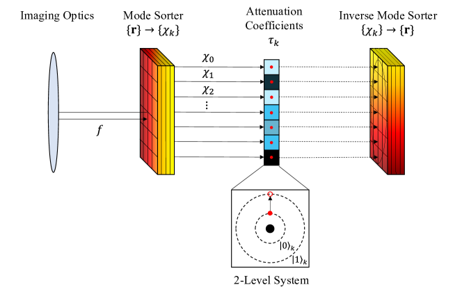
Figure 12: A schematic representation of a quantum mechanical formulation for the coronagraph operator. An arbitrary coronagraph is modelled as a unitary mode transformation from the focal plane to the eigenmodes of the coronagraph propagator. Each optical mode channel interacts with a two-level atom which either absorbs or transmits a photon with probability $1-|\tau_{k}|^{2}$ and $|\tau_{k}|^{2}$ respectively. Finally, the mode channels are transformed back into the spatial domain.

Consider a single optical eigenmode channel in isolation. Suppose the two-level system for this channel is in the ground state $\ket{0}_{k}$ and a single-photon state $\ket{\chi_{k}}$ of an eigenmode sent into the coronagraph. The resulting state is a superposition of the atom having absorbed and transmitted the photon such that,

$$\ket{\chi_{k}}\ket{0}_{k}\rightarrow\sqrt{1-|\tau_{k}|^{2}}\ket{0}\ket{1}_{k}+\tau\ket{\chi}\ket{0}_{k}$$

Since each optical mode channel is independent, we define the coronagraph operator to be the sum of connectors,

$$\hat{\mathcal{C}}=\sum_{k}\bigg{(}\sqrt{1-|\tau_{k}|^{2}}\ket{0,\mathbf{1}_{k}}+\tau_{k}\ket{\chi_{k},\mathbf{0}}\bigg{)}\bra{\chi_{k},\mathbf{0}}$$

where we have used the shorthand $\ket{\mathbf{1}_{k}}\in\mathcal{H}_{C}$ to represent the $k^{th}$ atom in the excited state with all other atoms in the ground state. Applying the coronagraph operator to an arbitrary single-photon optical state with the coronagraph in the ground state,

$$\hat{\mathcal{C}}\ket{\psi,\mathbf{0}}=\sum_{k}\innerproduct{\chi_{k}}{\psi}\bigg{(}\sqrt{1-|\tau_{k}|^{2}}\ket{0,\mathbf{1}_{k}}+\tau_{k}\ket{\chi_{k},\mathbf{0}}\bigg{)}$$

More generally, applying the coronagraph operator to a mixed single-photon state of the optical field given by $\hat{\rho}_{1}=\sum_{j}p_{j}\outerproduct{\psi_{j},\mathbf{0}}{\psi_{j},\mathbf{0}}$ where $\ket{\psi_{j}}$ are single-photon states yields,

$$\begin{split}\hat{\rho}^{\prime}=\hat{\mathcal{C}}\hat{\rho}_{1}\hat{\mathcal{C}}^{\dagger}=\sum_{j}p_{j}\sum_{k,k^{\prime}}&\innerproduct{\chi_{k}}{\psi_{j}}\bigg{(}\sqrt{1-|\tau_{k}|^{2}}\ket{0,\mathbf{1}_{k}}+\tau_{k}\ket{\chi_{k},\mathbf{0}}\bigg{)}\\ \times&\innerproduct{\psi_{j}}{\chi_{k^{\prime}}}\bigg{(}\sqrt{1-|\tau_{k^{\prime}}|^{2}}\bra{0,\mathbf{1}_{k}}+\tau^{*}_{k^{\prime}}\bra{\chi_{k^{\prime}},\mathbf{0}}\bigg{)}\end{split}$$

In the end, we only make measurements of the optical field. Thus we take the partial trace of the resulting state over the Hilbert space of the coronagraph $\mathcal{H}_{C}$

$$\begin{split}\hat{\rho}^{\prime}=&\text{Tr}\big{(}\hat{\rho}^{\prime}\big{)}_{C}\\ =&\sum_{j}p_{j}\sum_{k,k^{\prime}}\innerproduct{\chi_{k}}{\psi_{j}}\innerproduct{\psi_{j}}{\chi_{k^{\prime}}}\\ \times&\bigg{[}\sqrt{(1-|\tau_{k}|^{2})(1-|\tau_{k}^{\prime}|^{2})}\outerproduct{0}{0}+\tau_{k}\tau^{*}_{k^{\prime}}\outerproduct{\chi_{k}}{\chi_{k^{\prime}}}\bigg{]}\end{split}$$

which we see is separable into a vacuum term and single-photon term $\hat{\rho}^{\prime}=\alpha\outerproduct{0}{0}+\hat{\rho}^{\prime}_{1}$. The coronagraph operator can also be split into vacuum and single-photon coupling terms,

$$\hat{\mathcal{C}}=\hat{C}_{0}+\hat{C}_{1}$$

where $\hat{C}_{0}=\sum\sqrt{1-|\tau_{k}|^{2}}\outerproduct{0}{\chi_{k}}$ and $\hat{C}_{1}=\sum\tau_{k}\outerproduct{\chi_{k}}{\chi_{k}}$. We see that the resulting single-photon component $\hat{\rho}^{\prime}_{1}$ may be expressed as,

$$\hat{\rho}^{\prime}_{1}=\hat{C}_{1}\hat{\rho}_{1}\hat{C}_{1}^{\dagger}=\sum_{j}p_{j}\sum_{k,k^{\prime}}\innerproduct{\chi_{k}}{\psi_{j}}\innerproduct{\psi_{j}}{\chi_{k^{\prime}}}\tau_{k}\tau^{*}_{k^{\prime}}\outerproduct{\chi_{k}}{\chi_{k^{\prime}}}$$

Thus the effective coronagraph operator we define in Eqn. 13 is $\hat{C}\equiv\hat{C}_{1}$.

Appendix F The Fourier-Zernike Modes

The Zernike modes $\tilde{\psi}_{nm}$ constitute a PSF-matched basis over a circular pupil,

$$\tilde{\psi}_{nm}(u,\theta) \equiv R_{nm}(u)\Theta_{m}(\theta)\text{circ}(u)$$ (39a)

$$R_{nm}(u) \equiv\sum_{j=0}^{(n-|m|)/2}\frac{(-1)^{j}\sqrt{n+1}(n-j)!}{j![(n+m)/2-j]![(n-m)/2-j]!}u^{n-2j}$$ (39b)

$$\Theta_{m}(\theta) \equiv\begin{cases}\sqrt{2}\cos(|m|\theta)&(m>0)\\ 1&(m=0)\\ \sqrt{2}\sin(|m|\theta)&(m<0)\end{cases}$$ (39c)

$$\text{circ}(u) \equiv\begin{cases}1,&u\leq 1\\ 0,&u>1\end{cases}$$ (39d)

where the radial index range is $n=0,1,2,\ldots,\infty$. The angular index range is $m\in\mathcal{S}_{n}=\{-n,-n+2,\ldots,n-2,n\}$ for a given radial index. These modes are defined to satisfy orthonormality,

$$\int\tilde{\psi}^{*}_{nm}(u,\theta)\tilde{\psi}_{n^{\prime}m^{\prime}}(u,\theta)udud\theta=\delta_{nn^{\prime}}\delta_{mm^{\prime}}$$

The Fourier transform of the Zernike modes over the pupil are found in [44] to be,

$$\psi_{nm}(r,\phi)=i^{n+2|m|}\sqrt{n+1}\frac{J_{n+1}(2\pi r)}{\sqrt{\pi}r}\Theta_{m}(\phi)$$ (40)

Appendix G SPADE CFIM in the Fourier-Zernike Modes

In this section we derive the CFIM for a SPADE system configured to sort the Fourier-Zernike modes. In the first section, we express the complete CFIM free of approximations. In the second section, we consider the CFIM in the high contrast limit and prove that it equals the high-contrast QFIM.

G.1 Complete SPADE CFIM

The polar coordinates for the star and planet vectors are given by,

$$(r_{s},\phi_{s}) =\big{(}br_{\Delta},\phi_{\Delta}+\pi\big{)}$$

$$(r_{e},\phi_{e}) =\big{(}(1-b)r_{\Delta},\phi_{\Delta}\big{)}$$

where $r_{\Delta}\in[0,\infty)$ and $\phi_{\Delta}\in[0,2\pi)$. Let $P_{nm}=(1-b)p_{nm}(r_{s},\phi_{s})+bp_{nm}(r_{e},\phi_{e})$ be the probability of detecting a photon in Fourier-Zernike mode $n,m$ under the star-planet configuration where

$$p_{nm}(r,\phi)=|\Gamma_{nm}(r,\phi)|^{2}=\frac{1}{\pi}\bigg{[}\sqrt{n+1}\frac{J_{n+1}(2\pi r)}{\sqrt{\pi}r}\Theta_{m}(\phi)\bigg{]}^{2}$$

is the probability of detecting a photon in mode $n,m$ if a single point source is located at position $\mathbf{r}$. The CFIM contribution of each mode is given by,

$$\mathcal{I}^{r\phi}_{ij}[n,m]=\frac{\big{(}\partial_{\theta_{i}}P_{nm}\big{)}\big{(}\partial_{\theta_{j}}P_{nm}\big{)}}{P_{nm}}$$

where $\theta_{i}\in\{r_{\Delta},\phi_{\Delta}\}$. Thus, we begin by calculating the partial derivatives of the single-source mode probabilities,

$$p^{(r)}_{nm}(r,\phi) \equiv\partial_{r}p_{nm}(r,\phi)=2\bigg{(}\frac{J_{n+1}(2\pi r)}{r}\bigg{)}$$

$$\times \bigg{[}J_{n-1}(2\pi r)-J_{n-3}(2\pi r)\bigg{]}\bigg{(}\Theta_{m}(\phi)\bigg{)}^{2}$$ (41a)

$$p^{(\phi)}_{nm}(r,\phi) \equiv\partial_{\phi}p_{nm}(r,\phi)=4\bigg{(}\frac{J_{n+1}(2\pi r)}{r}\bigg{)}^{2}$$

$$\times (n+1)(-m)\cos(|m|\phi)\sin(|m|\phi)$$ (41b)

Applying the chain rule, the partial derivatives of the total mode probability is,

$$\partial_{r_{\Delta}}P_{nm} =(1-b)\partial_{r_{\Delta}}p_{nm}(br_{\Delta},\phi_{\Delta}+\pi)+b\partial_{r_{\Delta}}p_{nm}((1-b)r_{\Delta},\phi_{\Delta})$$

$$=b(1-b)\bigg{[}p^{(r)}_{nm}(br_{\Delta},\phi_{\Delta}+\pi)+p^{(r)}_{nm}((1-b)r_{\Delta},\phi_{\Delta})\bigg{]}$$

$$\partial_{\phi_{\Delta}}P_{nm} =(1-b)\partial_{\phi_{\Delta}}p_{nm}(br_{\Delta},\phi_{\Delta}+\pi)+b\partial_{\phi_{\Delta}}p_{nm}((1-b)r_{\Delta},\phi_{\Delta})$$

$$=(1-b)p^{(\phi)}_{nm}(br_{\Delta},\phi_{\Delta}+\pi)+bp^{(\phi)}_{nm}((1-b)r_{\Delta},\phi_{\Delta})$$

We refrain from substituting all elements into one equation as the resulting expression would be excessively long. However, the equations provided enable quick computation of the Fisher information contribution of each Zernike mode $\mathcal{I}_{ij}^{(r\phi)}[n,m]$. Drawing attention to Eq. 41, we see that $p^{(\phi)}_{nm}(r,\phi)=0$ for all $n,m$ when $\phi$ is an integer multiple of $\frac{\pi}{2}$. This implies that the CFI of the angular coordinate is zero when the separation axis of the star-planet system exactly coincides with the x-axis or the y-axis. These apparent ’singularities’ in the CFI can be neglected in practice because the probability of exact alignment along the x and y axes is infinitesimally small. That said, the disappearing CFI has non-negligible effects when considering a finite Zernike mode basis that is truncated at some arbitrarily large order. We find that a good rule of thumb for simulating the localization of point sources near the x and y axes is to use a truncated Zernike mode basis with the max radial being bounded by $n\gtrsim\lceil\frac{\pi}{2|\phi_{min}|}\rceil$ where $\phi_{min}$ is the minimum orientation angle (in radians) that the star-planet separation axis makes with either x or y axes. Alternatively, one may choose a lower mode truncation order and simply rotate the basis by $\pi/4$ radians halfway through the photon collection period to cover the singularities near the x,y axes.

G.2 SPADE CFIM in the High-Contrast Limit

In the high contrast limit where $b\rightarrow 0,\mathbf{r}_{s}\rightarrow 0,$ and $\mathbf{r}_{e}\rightarrow\mathbf{r}_{\Delta}$, the mode probabilities approach

$$P_{k}\rightarrow(1-b)p_{k}(0)+bp(\mathbf{r}_{\Delta})$$

where we have introduced the OSA/ANSI standard linear index of the Zernikes $k=(n(n+2)+m)/2$ for later convenience. Critically, for a PSF-matched SPADE basis, we have $p_{k}(0)=\delta_{k0}$. Moreover, inspecting Eq. 40, we see that the Fourier-Zernike modes are either purely imaginary or purely real based on the parity of $n+2|m|$. Since this is independent of the argument $\mathbf{r}$, we may re-define $\psi_{k}(\mathbf{r})\leftarrow i^{-(n+2|m|)}\psi_{k}(\mathbf{r})$ without loss of generality to make the Fourier-Zernike modes purely real. This allows us to write the magnitude squared of the correlation functions $|\Gamma_{k}(\mathbf{r})|^{2}=\Gamma_{k}(\mathbf{r})^{2}$ such that the CFIM terms adopt the convenient form,

$$\mathcal{I}_{k,ij}\rightarrow 4b^{2}\Gamma^{2}_{k}(\mathbf{r}_{\Delta})\,\frac{\bigg{(}\partial_{\theta_{i}}\Gamma_{k}(\mathbf{r}_{\Delta})\bigg{)}\bigg{(}\partial_{\theta_{j}}\Gamma_{k}(\mathbf{r_{\Delta}})\bigg{)}}{\delta_{k0}+b\Gamma^{2}_{k}(\mathbf{r}_{\Delta})}$$

Note that the presence of the Kronecker Delta in the denominator means the information contribution of the fundamental mode $k=0$ scales as $b^{2}$. Meanwhile, the information contribution of higher-order modes $k>0$ scales as $b$. Thus, in the high-contrast limit the SPADE CFIM approaches

$$\mathcal{I}_{ij}\rightarrow 4b\sum_{k>0}\bigg{(}\partial_{\theta_{i}}\Gamma_{k}(\mathbf{r}_{\Delta})\bigg{)}\bigg{(}\partial_{\theta_{j}}\Gamma_{k}(\mathbf{r}_{\Delta})\bigg{)}$$ (42)

G.3 Asymptotic Optimality of SPADE

To prove the optimality of SPADE for localization, we show that Eq. 42 is equal to the high-contrast QFIM of Eq. 30 for a circular aperture. We note that this derivation also constitutes a proof for the quantum optimality of the Zernike modes in the canonical balanced two-source localization problem involving a circular aperture. While the Zernikes have been conjectured as an optimal basis, the following constitutes, what we believe is, the first formal proof. We begin by evaluating the diagonal terms of the CFIM. Consider the infinite sum of radial derivatives

$$\sum_{k=0}^{\infty}(\partial_{r}\Gamma_{k}(r,\phi))^{2}$$

where in the Fourier-Zernike modes we have,

$$\partial_{r}\Gamma_{nm}(r,\phi)=\frac{\pi}{\sqrt{n+1}}\bigg{[}J_{n-1}(2\pi r)-J_{n+3}(2\pi r)\bigg{]}\Theta_{m}(\phi)$$

$$\sum_{n=0}^{\infty}\sum_{m\in\mathcal{S}_{n}}(\partial_{r}\Gamma_{nm}(r,\phi))^{2}$$

$$= \pi^{2}\sum_{n=0}^{\infty}\frac{1}{(n+1)}\bigg{[}J_{n-1}(2\pi r)-J_{n+3}(2\pi r)\bigg{]}^{2}\sum_{m\in\mathcal{S}_{n}}\bigg{(}\Theta_{m}(\phi)\bigg{)}^{2}$$

$$= \pi^{2}\sum_{n=0}^{\infty}\frac{1}{(n+1)}\bigg{[}J_{n-1}(2\pi r)-J_{n+3}(2\pi r)\bigg{]}^{2}\bigg{(}n+1\bigg{)}$$

$$= \sum_{n=0}^{\infty}\bigg{[}J_{n-1}(2\pi r)-J_{n+3}(2\pi r)\bigg{]}^{2}$$

$$= \pi^{2}$$

In the last line we have used the equation infinite sum below

$$\sum_{n=0}^{\infty}\bigg{[}J_{n-1}(x)-J_{n+3}(x)\bigg{]}^{2}=1\qquad\forall x\geq 0$$ (43)

Next consider the infinite sum of angular derivatives

$$\sum_{k=0}^{\infty}(\partial_{\phi}\Gamma_{k}(r,\phi))^{2}$$

where in the Fourier-Zernike modes we have,

$$\partial_{\phi}\Gamma_{nm}(r,\phi)=\sqrt{n+1}\frac{J_{n+1}(2\pi r)}{\pi r}\bigg{[}-m\Theta_{-m}(\phi)\bigg{]}$$

$$\sum_{n=0}^{\infty}\sum_{m\in\mathcal{S}_{n}}(\partial_{\phi}\Gamma_{nm}(r,\phi))^{2}$$

$$= \sum_{n=0}^{\infty}\frac{1}{(n+1)}\bigg{[}J_{n}(2\pi r)+J_{n+2}(2\pi r)\bigg{]}^{2}\sum_{m\in\mathcal{S}_{n}}m^{2}\Theta^{2}_{-m}(\phi)$$

$$= \sum_{n=0}^{\infty}\frac{1}{(n+1)}\bigg{[}J_{n}(2\pi r)+J_{n+2}(2\pi r)\bigg{]}^{2}\bigg{(}2\frac{n(n+1)(n+2)}{6}\bigg{)}$$

$$= \frac{1}{3}\sum_{n=0}^{\infty}n(n+2)\bigg{[}J_{n}(2\pi r)+J_{n+2}(2\pi r)\bigg{]}^{2}$$

$$= (\pi r)^{2}$$

where in the last line we have made use of the identity,

$$\frac{4}{3}\sum_{n=0}^{\infty}n(n+2)\bigg{[}J_{n}(x)+J_{n+2}(x)\bigg{]}^{2}=x^{2}\qquad\forall x\geq 0$$ (44)

Applying these terms to the high-contrast CFI of Eq. 42, we see that

$$\mathcal{I}^{(r\phi)}_{11} =4b\bigg{(}\pi^{2}-\big{(}\partial_{r_{\Delta}}\Gamma_{0}(r_{\Delta},\phi_{\Delta})\big{)}^{2}\bigg{)}$$

$$=4\pi^{2}b\bigg{(}1-\bigg{(}\frac{2J_{2}(2\pi r_{\Delta})}{\pi r_{\Delta}}\bigg{)}^{2}\bigg{)}$$ (45)

$$\mathcal{I}^{(r\phi)}_{22} =4b\bigg{(}(\pi r_{\Delta})^{2}-\big{(}\partial_{\phi_{\Delta}}\Gamma_{0}(r_{\Delta},\phi_{\Delta})\big{)}^{2}\bigg{)}$$

$$=4\pi^{2}br_{\Delta}^{2}$$ (46)

which are precisely the diagonal terms of the high-contrast QFIM shown in Eq. 30. The off-diagonal terms of the CFIM are equal to zero. This is easily shown by recognizing that the sums over the angular indices evaluate to zero.

$$\mathcal{I}^{(r\phi)}_{12} =\mathcal{I}^{(r\phi)}_{21}=4b\sum_{n=0}^{\infty}\sum_{m\in\mathcal{S}_{n}}\partial_{r}\Gamma_{nm}\partial_{\phi}\Gamma_{nm}$$

$$= 4b\sum_{n=0}^{\infty}\frac{J_{n+1}(2\pi r)}{r}\bigg{(}J_{n-1}(2\pi r)-J_{n+3}(2\pi r)\bigg{)}$$

$$\times\bigg{(}\sum_{m\in\mathcal{S}_{n}}-m\Theta_{m}(\phi)\Theta_{-m}(\phi)\bigg{)}$$

$$= 4b\sum_{n=0}^{\infty}\frac{J_{n+1}(2\pi r)}{r}\bigg{(}J_{n-1}(2\pi r)-J_{n+3}(2\pi r)\bigg{)}$$

$$\times\bigg{(}\sum_{m\in\mathcal{S}_{n}}-2m\sin(|m|\phi)\cos(|m|\phi)\bigg{)}$$

$$= 4b\sum_{n=0}^{\infty}\frac{J_{n+1}(2\pi r)}{r}\bigg{(}J_{n-1}(2\pi r)-J_{n+3}(2\pi r)\bigg{)}\times(0)$$

$$= 0$$

This concludes the proof.

Appendix H Asymptotic Optimality of the Perfect Coronagraph

In this section we will prove that the Perfect Coronagraph (PC) asymptotically approaches the QFIM in the high-contrast regime $b<<1$ between the star and the exoplanet. The coronagraph operator for the PC can be written as $\hat{C}=\hat{I}-\outerproduct{\psi_{0}}{\psi_{0}}$ where $\hat{\mathds{1}}$ is the identity. Therefore the field state post-nulling of the fundamental PSF mode is given by,

$$\hat{\rho}^{\prime} =(\hat{\mathds{1}}-\outerproduct{\psi_{0}}{\psi_{0}})\hat{\rho}(\hat{\mathds{1}}-\outerproduct{\psi_{0}}{\psi_{0}})$$

$$=\hat{\rho}+\matrixelement{\psi_{0}}{\hat{\rho}}{\psi_{0}}\outerproduct{\psi_{0}}{\psi_{0}}-\outerproduct{\psi_{0}}{\psi_{0}}\hat{\rho}-\hat{\rho}\outerproduct{\psi_{0}}{\psi_{0}}$$

where $\ket{\psi_{0}}$ is the single photon state in the fundamental mode. Our goal is to determine the CFI for a direct imaging measurement $\bigg{\{}\hat{\Pi}_{\mathbf{r}}=\outerproduct{\mathbf{r}}{\mathbf{r}}\bigg{\}}$ on the nulled density operator. First we find the probability of detecting a photon at location $\mathbf{r}$ on the image plane.

$$p(\mathbf{r})= \matrixelement{\mathbf{r}}{\hat{\rho}^{\prime}}{\mathbf{r}}$$

$$= \rho(\mathbf{r})+\matrixelement{\psi_{0}}{\hat{\rho}}{\psi_{0}}|\psi_{0}(\mathbf{r})|^{2}$$

$$-\psi_{0}(\mathbf{r})\matrixelement{\psi_{0}}{\hat{\rho}}{\mathbf{r}}-\psi^{*}_{0}(\mathbf{r})\matrixelement{\mathbf{r}}{\hat{\rho}}{\psi_{0}}$$

$$= \rho(\mathbf{r})+\matrixelement{\psi_{0}}{\hat{\rho}}{\psi_{0}}|\psi_{0}(\mathbf{r})|^{2}-2\Re{\psi_{0}(\mathbf{r})\matrixelement{\psi_{0}}{\hat{\rho}}{\mathbf{r}}}$$

which expands to

$$\begin{split}p(\mathbf{r})=&(1-b)|\psi_{0}(\mathbf{r}-\mathbf{r}_{s})|^{2}+b|\psi_{0}(\mathbf{r}-\mathbf{r}_{e})|^{2}\\ &+|\psi_{0}(\mathbf{r})|^{2}\bigg{(}(1-b)|\Gamma_{0}(\mathbf{r}_{s})|^{2}+b|\Gamma_{0}(\mathbf{r}_{e})|^{2}\bigg{)}\\ &-2\real\{\psi_{0}(\mathbf{r})\bigg{(}(1-b)\Gamma_{0}(\mathbf{r}_{s})\psi^{*}_{0}(\mathbf{r}-\mathbf{r}_{s})\\ &+b\Gamma_{0}(\mathbf{r}_{e})\psi^{*}_{0}(\mathbf{r}-\mathbf{r}_{e})\bigg{)}\bigg{\}}\end{split}$$

In the limit of high contrast $b<<1$ where $\mathbf{r}_{s}\rightarrow 0$ and $\mathbf{r}_{e}\rightarrow\mathbf{r}_{\Delta}$, the probability is well-approximated by,

$$\begin{split}p(\mathbf{r})\approx&2(1-b)|\psi_{0}(\mathbf{r})|^{2}+b|\psi_{0}(\mathbf{r}-\mathbf{r}_{\Delta})|^{2}+b|\psi_{0}(\mathbf{r})|^{2}|\Gamma_{0}(\mathbf{r}_{\Delta})|^{2}\\ &-2\Re{\psi_{0}(\mathbf{r})\bigg{(}(1-b)\psi^{*}_{0}(\mathbf{r})+b\Gamma_{0}(\mathbf{r}_{\Delta})\psi^{*}_{0}(\mathbf{r}-\mathbf{r}_{\Delta})\bigg{)}}\end{split}$$

Assuming a real-valued PSF, this further reduces to

$$p(\mathbf{r})\approx b\bigg{[}\psi^{2}_{0}(\mathbf{r}-\mathbf{r}_{\Delta})+\psi^{2}_{0}(\mathbf{r})\Gamma^{2}_{0}(\mathbf{r}_{\Delta})-2\psi_{0}(\mathbf{r})\Gamma_{0}(\mathbf{r}_{\Delta})\psi_{0}(\mathbf{r}-\mathbf{r}_{\Delta})\bigg{]}$$

$$\approx b\bigg{[}\psi_{0}(\mathbf{r}-\mathbf{r}_{\Delta})-\Gamma_{0}(\mathbf{r}_{\Delta})\psi_{0}(\mathbf{r})\bigg{]}^{2}$$

Let us now define the real-valued proxy correlation function

$$\Gamma(\mathbf{r};\mathbf{r}_{\Delta})\equiv\sqrt{b}\bigg{[}\psi_{0}(\mathbf{r}-\mathbf{r}_{\Delta})-\Gamma_{0}(\mathbf{r}_{\Delta})\psi_{0}(\mathbf{r})\bigg{]}$$

such that $p(\mathbf{r})\approx\Gamma^{2}(\mathbf{r};\mathbf{r}_{\Delta})$. Doing so allows us to write the CFI matrix in the convenient form,

$$\mathcal{I}_{ij}\approx\int d^{2}r\frac{(\partial_{\theta_{i}}\Gamma^{2})(\partial_{\theta_{j}}\Gamma^{2})}{\Gamma^{2}}=4\int d^{2}r(\partial_{\theta_{i}}\Gamma)(\partial_{\theta_{j}}\Gamma)$$

Note that $\Gamma(\mathbf{r};\mathbf{r}_{\Delta})$ is proportional to the optical field induced by a shifted PSF minus its component in the fundamental mode. Moreover, the shifted PSF admits an expansion in a PSF-matched orthonormal basis,

$$\psi_{0}(\mathbf{r}-\mathbf{r}_{\Delta})=\sum_{k=0}^{\infty}\Gamma_{k}(\mathbf{r}_{\Delta})\psi_{k}(\mathbf{r})$$

such that we may express the proxy correlation function as,

$$\Gamma(\mathbf{r};\mathbf{r}_{\Delta})=\sqrt{b}\sum_{k>0}\Gamma_{k}(\mathbf{r}_{\Delta})\psi_{k}(\mathbf{r})$$

Substituting this expression into the CFI and invoking the orthogonality of the modes, we have

$$\mathcal{I}_{ij}\rightarrow 4b\sum_{k>0}\big{(}\partial_{\theta_{i}}\Gamma_{k}(\mathbf{r}_{\Delta})\big{)}\big{(}\partial_{\theta_{j}}\Gamma_{k}(\mathbf{r}_{\Delta})\big{)}$$

which we immediately recognize as Eq. 42, the CFIM of SPADE in the high-contrast limit. We proved Eq. 42 approaches QFIM in Appendix G.2. Hence the Perfect coronagraph is quantum optimal.

Appendix I CCE for Direct-Imaging Coronagraphs

For coronagraphs like the PC, PIAACMC, and VC which achieve total nulling of an on-axis star, there is no sensible application of the definition of the Classical Chernoff Exponent provided in Eq. 20 since the post-nulling probability $p^{\prime}_{0}(\mathbf{r})=\matrixelement{\mathbf{r}}{\hat{C}\hat{\rho}_{0}\hat{C}^{\dagger}}{\mathbf{r}}$ goes to zero. In these systems, the only possible type of detection errors that can occur are false-negatives. Therefore, we take the probability of error to be the probability that all photons entering the pupil from hypothesis $\hat{\rho}_{1}$ are blocked by the coronagraph (i.e. none make it to the image plane).

$$P_{e}=\big{[}1-\text{Tr}(\hat{C}\hat{\rho}_{1}\hat{C}^{\dagger})\big{]}^{N}$$

Rewriting the probability of error as,

$$P_{e}=e^{-N\xi_{C}}=e^{N\log(1-\text{Tr}(\hat{C}\hat{\rho}_{1}\hat{C}^{\dagger}))}$$

we see that the CCE for a coronagraph capable of total on-axis nulling is given by,

$$\xi_{C}=-\log(1-\text{Tr}(\hat{C}\hat{\rho}_{1}\hat{C}^{\dagger}))$$

where the probability of photon detection at the image plane can be expanded as,

$$\text{Tr}(\hat{C}\hat{\rho}_{1}\hat{C}^{\dagger})=\sum_{k}|\tau_{k}|^{2}\bigg{[}(1-b)|\innerproduct{\chi_{k}}{\psi_{0}(\mathbf{r}_{s})}|^{2}+b|\innerproduct{\chi_{k}}{\psi_{0}(\mathbf{r}_{e})}|^{2}\bigg{]}$$

In the high-contrast regime, this reduces to,

$$\text{Tr}(\hat{C}\hat{\rho}_{1}\hat{C}^{\dagger})\approx\sum_{k}|\tau_{k}|^{2}\bigg{[}(1-b)|\innerproduct{\chi_{k}}{\psi_{0}}|^{2}+b|\innerproduct{\chi_{k}}{\psi_{0}(\mathbf{r}_{\Delta})}|^{2}\bigg{]}$$

Without loss of generality, we may define $\chi_{0}(\mathbf{r})=\psi_{0}(\mathbf{r})$ which has $\tau_{0}=0$ since $\ket{\psi_{0}}$ lives in the null space of $\hat{C}$. Then the high-contrast photon detection probability becomes,

$$\text{Tr}(\hat{C}\hat{\rho}_{1}\hat{C}^{\dagger}) \approx b\sum_{k}|\tau_{k}|^{2}|\innerproduct{\chi_{k}}{\psi_{0}(\mathbf{r}_{\Delta})}|^{2}$$

$$=b\text{Tr}(\hat{C}\outerproduct{\psi_{0}(\mathbf{r}_{\Delta})}{\psi_{0}(\mathbf{r}_{\Delta})}\hat{C}^{\dagger})$$

Inserting the high-contrast approximation into our definition of the CCE and Taylor expanding the logarithm, we arrive at the high-contrast CCE limit

$$\xi_{C}\xrightarrow[]{b<<1}b\text{Tr}\big{(}\hat{C}\outerproduct{\psi_{0}(\mathbf{r}_{\Delta})}{\psi_{0}(\mathbf{r}_{\Delta})}\hat{C}^{\dagger}\big{)}$$

We see that the high-contrast CCE is proportional to the probability that a photon emitted by a single point source located at $\mathbf{r}_{\Delta}$ arrives at the image plane. The term $\text{Tr}(\hat{C}\outerproduct{\psi_{0}(\mathbf{r}_{\Delta})}{\psi_{0}(\mathbf{r}_{\Delta})}\hat{C}^{\dagger})$ is equivalent to what is commonly called the ’throughput’ of the coronagraph. The proportionality factor $b$ indicates that the high-contrast CCE can be thought of as the probability that an exoplanet photon reaches the detector.

Appendix J CFIM for Direct Imaging Coronagraphs

The probability density over the image plane for detecting a photon at location $\mathbf{r}$ after propagating the state through a general coronagraph is given by,

$$p(\mathbf{r})= \matrixelement{\mathbf{r}}{\hat{C}\hat{\rho}\hat{C}^{\dagger}}{\mathbf{r}}$$

$$= \sum_{kk^{\prime}}\tau_{k}\tau^{*}_{k^{\prime}}\chi_{k}(\mathbf{r})\chi^{*}_{k^{\prime}}(\mathbf{r})$$

$$\times\bigg{[}(1-b)\Gamma_{k}(\mathbf{r}_{s})\Gamma^{*}_{k^{\prime}}(\mathbf{r}_{s})+b\Gamma_{k}(\mathbf{r}_{e})\Gamma^{*}_{k^{\prime}}(\mathbf{r}_{e})\bigg{]}$$

where here we use the correlation function with the coronagraph eigenmodes

$$\Gamma_{k}(\mathbf{s})=\innerproduct{\chi_{k}}{\psi_{0}(\mathbf{s})}$$

For a coronagraph that rejects the fundamental mode such that $\ket{\psi_{0}}\in\text{Null}(\hat{C})$ we define the first eigenmode as $\chi_{0}(\mathbf{r})\equiv\psi_{0}(\mathbf{r})$. Taking the high contrast limit, the probability density is well approximated by,

$$p(\mathbf{r})\approx b\bigg{|}\sum_{k>0}\tau_{k}\Gamma_{k}(\mathbf{r}_{\Delta})\chi_{k}(\mathbf{r})\bigg{|}^{2}$$

which we recognize as the weighted expansion of the shifted PSF in the eigenmode basis of the coronagraph operator. The expansion coefficients are further modulated by the transmission of each mode. Unfortunately, this form for the probability is does not generally lend itself to a reduced expression for the high-contrast direct imaging CFIM. However, we conjecture that the direct imaging CFIM is bounded from above by,

$$\mathcal{I}_{ij}\stackrel{{\scriptstyle?}}{{\leq}}b\sum_{k>0}|\tau_{k}|^{2}\frac{\big{(}\partial_{\theta_{i}}p_{k}(\mathbf{r}_{\Delta})\big{)}\big{(}\partial_{\theta_{j}}p_{k}(\mathbf{r}_{\Delta})\big{)}}{p_{k}(\mathbf{r}_{\Delta})}$$

which is the high-contrast CFIM of a SPADE measurement in the eigenmodes of the coronagraph with $p_{k}(\mathbf{r}_{\Delta})=|\innerproduct{\chi_{k}}{\psi_{0}(\mathbf{r}_{\Delta})}|^{2}$. The information contribution of each mode is weighted by the squared magnitude of the transmission coefficient.

Appendix K Proof of Equations 43 and 44

K.1 Useful Bessel Function Identities

The proofs of Eq 43 and Eq 44 makes use of the following helpful Bessel function identities.

$$J_{-n}(x)=(-1)^{n}J_{n}(x)\qquad n\geq 0$$ (47a)

$$2\frac{nJ_{n}(x)}{x}=J_{n-1}(x)+J_{n+1}(x)$$ (47b)

$$2\frac{dJ_{n}(x)}{dx}=J_{n-1}(x)-J_{n+1}(x)$$ (47c)

$$2\sum_{n=0}^{\infty}J^{2}_{n}(x)=1+J_{0}^{2}(x)$$ (47d)

$$2\sum_{n=1}^{\infty}J_{n}(x)J_{2m+n}(x)=-\sum_{k=n}^{2m}(-1)^{n}J_{n}(x)J_{2m-n}\qquad(m\geq 1)$$ (47e)

These identities can be found either on the Digital Library of Mathematical Functions: (47a [45, (10.4.1)]), (47b [45, (10.6.1)]), (47c [45, (10.6.1)]), (47d [45, (10.23.3)]), (47e [45, (10.23.4)])

K.2 Proof of Equation 43

We drop the arguments of the Bessel functions for notational convenience.

$$\sum_{n=0}^{\infty}\bigg{[}J_{n-1}-J_{n+3}\bigg{]}^{2} =\sum_{n=0}^{\infty}J^{2}_{n-1}+\sum_{n=0}^{\infty}J^{2}_{n+3}-2\sum_{n=0}^{\infty}J_{n-1}J_{n+3}$$

We evaluate each sum independently and combine them at the end.

$$\sum_{n=0}^{\infty}J^{2}_{n-1} =\sum_{n=-1}^{\infty}J^{2}_{n}$$

$$=J^{2}_{-1}+\sum_{n=0}^{\infty}J^{2}_{n}$$

Next, use 47a and equation 47d.

$$=J^{2}_{1}+\bigg{[}\frac{1+J^{2}_{0}}{2}\bigg{]}$$

$$\sum_{n=0}^{\infty}J^{2}_{n+3} =-J^{2}_{0}-J^{2}_{1}-J^{2}_{2}+\sum_{n=0}J^{2}_{n}$$

Next, use equation 47d.

$$=-J^{2}_{0}-J^{2}_{1}-J^{2}_{2}+\bigg{[}\frac{1+J^{2}_{0}}{2}\bigg{]}$$

$$-2\sum_{n=0}^{\infty}J_{n-1}J_{n+3} =-2J_{-1}J_{3}-2J_{0}J_{4}-2\sum_{n=1}^{\infty}J_{n}J_{n+4}$$

Next, use 47a with $$J_{-1}(x)=(-1)J_{1}(x)$$ and 47e with m=2

$$=2J_{1}J_{3}-2J_{0}J_{4}+\bigg{[}\sum_{k=0}^{4}(-1)^{k}J_{k}J_{4-k}\bigg{]}$$

$$=2J_{1}J_{3}-2J_{0}J_{4}+\bigg{[}J_{0}J_{4}-J_{1}J_{3}+J_{2}J_{2}-J_{3}J_{1}-J_{4}J_{0}\bigg{]}$$

$$=J^{2}_{2}$$

Summing all terms we find the following.

$$\mathcal{J}_{rr} =J^{2}_{1}+\bigg{[}\frac{1+J^{2}_{0}}{2}\bigg{]}-J^{2}_{0}-J^{2}_{1}-J^{2}_{2}+\bigg{[}\frac{1+J^{2}_{0}}{2}\bigg{]}+J^{2}_{2}$$

$$=1$$

K.3 Proof of Equation 44

We drop the arguments of the Bessel functions for notational convenience.

$$\frac{4}{3}\sum_{n=0}^{\infty}n(n+2)\bigg{[}J_{n}(x)+J_{n+2}(x)\bigg{]}^{2} =\frac{4}{3}\sum_{n=0}^{\infty}n(n+2)J^{2}_{n}+2n(n+2)J_{n}J_{n+2}+n(n+2)J^{2}_{n+2}$$

We will evaluate each sum independently.

$$\sum_{n=0}^{\infty}n(n+2)J^{2}_{n} =\sum_{n=0}^{\infty}(nJ_{n})^{2}+\sum_{n=0}^{\infty}2nJ_{n}^{2}$$

Apply equation 47b to the first sum above.

$$=\sum_{n=0}^{\infty}\frac{x^{2}}{4}(J_{n-1}+J_{n+1})^{2}+2\sum_{n=0}^{\infty}nJ_{n}^{2}$$

$$=\frac{x^{2}}{4}\bigg{[}\sum_{n=0}^{\infty}J^{2}_{n-1}+2J_{n-1}J_{n+1}+J^{2}_{n+1}\bigg{]}+2\sum_{n=0}^{\infty}nJ_{n}^{2}$$

Apply equation 47d on the squared Bessel terms.

$$=\frac{x^{2}}{4}\bigg{[}J_{-1}^{2}+\frac{1}{2}(1+J^{2}_{0})+\frac{1}{2}(1-J^{2}_{0})+2\sum_{n=0}^{\infty}J_{n-1}J_{n+1}\bigg{]}+2\sum_{n=0}^{\infty}nJ_{n}^{2}$$

Apply equation 47a to the $$J_{-1}$$ term.

$$=\frac{x^{2}}{4}\bigg{[}1+J^{2}_{1}+2\sum_{n=0}^{\infty}J_{n-1}J_{n+1}\bigg{]}+2\sum_{n=0}^{\infty}nJ_{n}^{2}$$

$$=\frac{x^{2}}{4}\bigg{[}1+J^{2}_{1}+2J_{-1}J_{1}+2J_{0}J_{2}+2\sum_{n=2}^{\infty}J_{n-1}J_{n+1}\bigg{]}+2\sum_{n=0}^{\infty}nJ_{n}^{2}$$

Apply equation 47a to the $$J_{-1}$$ term.

$$=\frac{x^{2}}{4}\bigg{[}1-J^{2}_{1}+2J_{0}J_{2}+2\sum_{n=1}^{\infty}J_{n}J_{n+2}\bigg{]}+2\sum_{n=0}^{\infty}nJ_{n}^{2}$$

Apply equation 47e to the infinite sum with $$m=1$$.

$$=\frac{x^{2}}{4}\bigg{[}1-J^{2}_{1}+2J_{0}J_{2}-\sum_{n=0}^{2}(-1)^{n}J_{n}J_{2-n}\bigg{]}+2\sum_{n=0}^{\infty}nJ_{n}^{2}$$

Apply equation 47a to the $$J_{-1}$$ term.

$$=\frac{x^{2}}{4}\bigg{[}1-J^{2}_{1}+2J_{0}J_{2}-\big{(}2J_{0}J_{2}-J^{2}_{1}\big{)}\bigg{]}+2\sum_{n=0}^{\infty}nJ_{n}^{2}$$

$$=\frac{x^{2}}{4}+2\sum_{n=0}^{\infty}nJ_{n}^{2}$$

On the way, we have found the identity $$\sum_{n=0}^{\infty}(nJ_{n})^{2}=\frac{x^{2}}{4}$$.

and the identity $$2\sum_{n=0}^{\infty}J_{n-1}J_{n+1}=-J^{2}_{1}$$

$$\sum_{n=0}^{\infty}2n(n+2)J_{n}J_{n+2} =2\sum_{n=0}^{\infty}\frac{x^{2}}{4}(J_{n-1}+J_{n+1})(J_{n+1}+J_{n+3})$$

Apply equation 47b to each index-bessel pairs in the sum and expand terms.

$$=2\sum_{n=0}^{\infty}\frac{x^{2}}{4}\bigg{[}J_{n-1}J_{n+1}+J_{n-1}J_{n+3}+J^{2}_{n+1}+J_{n+1}J_{n+3}\bigg{]}$$

Each term is a product of bessel functions with an even difference in index.

$$=\frac{x^{2}}{4}\sum_{n=0}^{\infty}2\bigg{[}J_{n-1}J_{n+1}+J_{n-1}J_{n+3}+J^{2}_{n+1}+J_{n+1}J_{n+3}\bigg{]}$$

$$=\frac{x^{2}}{4}\bigg{[}2\sum_{n=0}^{\infty}J_{n-1}J_{n+1}+2\sum_{n=0}^{\infty}J_{n-1}J_{n+3}+2\sum_{n=0}^{\infty}J^{2}_{n+1}+2\sum_{n=0}^{\infty}J_{n+1}J_{n+3}\bigg{]}$$

Apply the identity found for term 1 and equation 47d to term 3.

$$=\frac{x^{2}}{4}\bigg{[}(-J^{2}_{1})+2\bigg{(}J_{-1}J_{3}+J_{0}J_{4}+\sum_{n=1}^{\infty}J_{n}J_{n+4}\bigg{)}+\bigg{(}1-J^{2}_{0}\bigg{)}+2\sum_{n=1}^{\infty}J_{n}J_{n+2}\bigg{]}$$

Apply equation 47e to term 2 with $$(m=1) (m=2)$$ and term 4 .

$$=\frac{x^{2}}{4}\bigg{[}(1-J^{2}_{0}-J^{2}_{1})+\bigg{(}2J_{-1}J_{3}+2J_{0}J_{4}-\sum_{n=0}^{4}(-1)^{n}J_{n}J_{4-n}\bigg{)}-\sum_{n=0}^{2}(-1)^{n}J_{n}J_{2-n}\bigg{]}$$

$$=\frac{x^{2}}{4}\bigg{[}(1-J^{2}_{0}-J^{2}_{1})+\bigg{(}2J_{-1}J_{3}+2J_{0}J_{4}-(2J_{0}J_{4}-2J_{1}J_{3}+J^{2}_{2})\bigg{)}-\bigg{(}2J_{0}J_{2}-J^{2}_{1}\bigg{)}\bigg{]}$$

Apply equation 47a to terms involving $$J_{-1}$$.

$$=\frac{x^{2}}{4}\bigg{[}1-J^{2}_{0}-J^{2}_{1}-2J_{1}J_{3}+2J_{0}J_{4}-2J_{0}J_{4}+2J_{1}J_{3}-J^{2}_{2}-2J_{0}J_{2}+J^{2}_{1}\bigg{]}$$

$$=\frac{x^{2}}{4}\bigg{[}1-J^{2}_{0}-J^{2}_{2}-2J_{0}J_{2}\bigg{]}$$

$$=\frac{x^{2}}{4}\bigg{[}1-\bigg{(}J_{0}+J_{2}\bigg{)}^{2}\bigg{]}$$

Apply equation 47b.

$$=\frac{x^{2}}{4}\bigg{[}1-\bigg{(}\frac{2}{x}J_{1}\bigg{)}\bigg{]}$$

$$=\frac{x^{2}}{4}-J^{2}_{1}$$

$$\sum_{n=0}^{\infty}n(n+2)J^{2}_{n+2} =\sum_{n=0}^{\infty}((n+2)-2)(n+2)J^{2}_{n+2}$$

$$=\sum_{n=0}^{\infty}(n+2)^{2}J^{2}_{n+2}-2\sum_{n=0}^{\infty}(n+2)J^{2}_{n+2}$$

$$=\bigg{[}-J^{2}_{1}+\sum_{n=0}^{\infty}(nJ_{n})^{2}\bigg{]}-2\bigg{[}-J^{2}_{1}+\sum_{n=0}^{\infty}nJ^{2}_{n}\bigg{]}$$

Apply the identity found for the sum of squared bessel times index.

$$=J^{2}_{1}+\frac{x^{2}}{4}-2\sum_{n=0}^{\infty}nJ^{2}_{n}$$

Summing all of the terms we have the desired result

$$\frac{4}{3}\bigg{[}\bigg{(}\frac{x^{2}}{4}+2\sum_{n=0}^{\infty}nJ_{n}^{2}\bigg{)}+\bigg{(}\frac{x^{2}}{4}-J^{2}_{1}\bigg{)}+\bigg{(}J^{2}_{1}+\frac{x^{2}}{4}-2\sum_{n=0}^{\infty}nJ^{2}_{n}\bigg{)}\bigg{]}$$

$$= \frac{4}{3}\bigg{[}\frac{3}{4}x^{2}\bigg{]}$$

$$= x^{2}$$

References

• [1] M A C Perryman. Extra-solar planets. Reports on Progress in Physics, 63(8):1209, aug 2000.
• [2] M. A. C. Perryman. Towards the detection of earth-like extra-solar planets. In Peter A. Shaver, Luigi DiLella, and Alvaro Giménez, editors, Astronomy, Cosmology and Fundamental Physics, pages 371–380, Berlin, Heidelberg, 2003. Springer Berlin Heidelberg.
• [3] W. A. Traub and B. R. Oppenheimer. Direct Imaging of Exoplanets, pages 111–156. Seager, S., 2010.
• [4] Rachel B Fernandes, Gijs D Mulders, Ilaria Pascucci, Christoph Mordasini, and Alexandre Emsenhuber. Hints for a turnover at the snow line in the giant planet occurrence rate. The Astrophysical Journal, 874(1):81, 2019.
• [5] Galen J Bergsten, Ilaria Pascucci, Gijs D Mulders, Rachel B Fernandes, and Tommi T Koskinen. The demographics of kepler’s earths and super-earths into the habitable zone. The Astronomical Journal, 164(5):190, 2022.
• [6] Carole Aimé and R Soummer. The usefulness and limits of coronagraphy in the presence of pinned speckles. The Astrophysical Journal, 612(1):L85, 2004.
• [7] Céline Cavarroc, Anthony Boccaletti, Pierre Baudoz, Thierry Fusco, and Daniel Rouan. Fundamental limitations on earth-like planet detection with extremely large telescopes. Astronomy & Astrophysics, 447(1):397–403, 2006.
• [8] O. Guyon, E. A. Pluzhnik, M. J. Kuchner, B. Collins, and S. T. Ridgway. Theoretical limits on extrasolar terrestrial planet detection with coronagraphs. The Astrophysical Journal Supplement Series, 167(1):81, nov 2006.
• [9] Ruslan Belikov, Dan Sirbu, Jeffrey B. Jewell, Olivier Guyon, and Christopher C. Stark. Theoretical performance limits for coronagraphs on obstructed and unobstructed apertures: how much can current designs be improved? In Stuart B. Shaklan and Garreth J. Ruane, editors, Techniques and Instrumentation for Detection of Exoplanets X, volume 11823, page 118230W. International Society for Optics and Photonics, SPIE, 2021.
• [10] Mankei Tsang, Ranjith Nair, and Xiao-Ming Lu. Quantum theory of superresolution for two incoherent optical point sources. Phys. Rev. X, 6:031033, Aug 2016.
• [11] Shan Zheng Ang, Ranjith Nair, and Mankei Tsang. Quantum limit for two-dimensional resolution of two incoherent optical point sources. Phys. Rev. A, 95:063847, Jun 2017.
• [12] Sudhakar Prasad. Quantum limits on localizing point objects against a uniformly bright disk. Phys. Rev. A, 107:032427, Mar 2023.
• [13] J. Řehaček, Z. Hradil, B. Stoklasa, M. Paúr, J. Grover, A. Krzic, and L. L. Sánchez-Soto. Multiparameter quantum metrology of incoherent point sources: Towards realistic superresolution. Phys. Rev. A, 96:062107, Dec 2017.
• [14] Zachary Dutton, Ronan Kerviche, Amit Ashok, and Saikat Guha. Attaining the quantum limit of superresolution in imaging an object’s length via predetection spatial-mode sorting. Phys. Rev. A, 99:033847, Mar 2019.
• [15] Zixin Huang and Cosmo Lupo. Quantum hypothesis testing for exoplanet detection and spectroscopy. In Optica Quantum 2.0 Conference and Exhibition, page QM2B.5. Optica Publishing Group, 2023.
• [16] Ugo Zanforlin, Cosmo Lupo, Peter W. R. Connolly, Pieter Kok, Gerald S. Buller, and Zixin Huang. Optical quantum super-resolution imaging and hypothesis testing. Nature Communications, 13(1), September 2022.
• [17] LUVOIR Team et al. The luvoir mission concept study final report. arXiv preprint arXiv:1912.06219, 2019.
• [18] B. Scott Gaudi, Sara Seager, Bertrand Mennesson, Alina Kiessling, Keith Warfield, Kerri Cahoy, John T. Clarke, Shawn Domagal-Goldman, Lee Feinberg, Olivier Guyon, Jeremy Kasdin, Dimitri Mawet, Peter Plavchan, Tyler Robinson, Leslie Rogers, Paul Scowen, Rachel Somerville, Karl Stapelfeldt, Christopher Stark, Daniel Stern, Margaret Turnbull, Rashied Amini, Gary Kuan, Stefan Martin, Rhonda Morgan, David Redding, H. Philip Stahl, Ryan Webb, Oscar Alvarez-Salazar, William L. Arnold, Manan Arya, Bala Balasubramanian, Mike Baysinger, Ray Bell, Chris Below, Jonathan Benson, Lindsey Blais, Jeff Booth, Robert Bourgeois, Case Bradford, Alden Brewer, Thomas Brooks, Eric Cady, Mary Caldwell, Rob Calvet, Steven Carr, Derek Chan, Velibor Cormarkovic, Keith Coste, Charlie Cox, Rolf Danner, Jacqueline Davis, Larry Dewell, Lisa Dorsett, Daniel Dunn, Matthew East, Michael Effinger, Ron Eng, Greg Freebury, Jay Garcia, Jonathan Gaskin, Suzan Greene, John Hennessy, Evan Hilgemann, Brad Hood, Wolfgang Holota, Scott Howe, Pei Huang, Tony Hull, Ron Hunt, Kevin Hurd, Sandra Johnson, Andrew Kissil, Brent Knight, Daniel Kolenz, Oliver Kraus, John Krist, Mary Li, Doug Lisman, Milan Mandic, John Mann, Luis Marchen, Colleen Marrese-Reading, Jonathan McCready, Jim McGown, Jessica Missun, Andrew Miyaguchi, Bradley Moore, Bijan Nemati, Shouleh Nikzad, Joel Nissen, Megan Novicki, Todd Perrine, Claudia Pineda, Otto Polanco, Dustin Putnam, Atif Qureshi, Michael Richards, A. J. Eldorado Riggs, Michael Rodgers, Mike Rud, Navtej Saini, Dan Scalisi, Dan Scharf, Kevin Schulz, Gene Serabyn, Norbert Sigrist, Glory Sikkia, Andrew Singleton, Stuart Shaklan, Scott Smith, Bart Southerd, Mark Stahl, John Steeves, Brian Sturges, Chris Sullivan, Hao Tang, Neil Taras, Jonathan Tesch, Melissa Therrell, Howard Tseng, Marty Valente, David Van Buren, Juan Villalvazo, Steve Warwick, David Webb, Thomas Westerhoff, Rush Wofford, Gordon Wu, Jahning Woo, Milana Wood, John Ziemer, Giada Arney, Jay Anderson, Jesús Maíz-Apellániz, James Bartlett, Ruslan Belikov, Eduardo Bendek, Brad Cenko, Ewan Douglas, Shannon Dulz, Chris Evans, Virginie Faramaz, Y. Katherina Feng, Harry Ferguson, Kate Follette, Saavik Ford, Miriam García, Marla Geha, Dawn Gelino, Ylva Götberg, Sergi Hildebrandt, Renyu Hu, Knud Jahnke, Grant Kennedy, Laura Kreidberg, Andrea Isella, Eric Lopez, Franck Marchis, Lucas Macri, Mark Marley, William Matzko, Johan Mazoyer, Stephan McCandliss, Tiffany Meshkat, Christoph Mordasini, Patrick Morris, Eric Nielsen, Patrick Newman, Erik Petigura, Marc Postman, Amy Reines, Aki Roberge, Ian Roederer, Garreth Ruane, Edouard Schwieterman, Dan Sirbu, Christopher Spalding, Harry Teplitz, Jason Tumlinson, Neal Turner, Jessica Werk, Aida Wofford, Mark Wyatt, Amber Young, and Rob Zellem. The habitable exoplanet observatory (habex) mission concept study final report, 2020.
• [19] Niyati Desai, Lorenzo König, Emiel Por, Roser Juanola-Parramon, Ruslan Belikov, Iva Laginja, Olivier Guyon, Laurent Pueyo, Kevin Fogarty, Olivier Absil, Lisa Altinier, Pierre Baudoz, Alexis Bidot, Markus Johannes Bonse, Kimberly Bott, Bernhard Brandl, Alexis Carlotti, Sarah L. Casewell, Elodie Choquet, Nicolas B. Cowan, David Doelman, J. Fowler, Timothy D. Gebhard, Yann Gutierrez, Sebastiaan Y. Haffert, Olivier Herscovici-Schiller, Adrien Hours, Matthew Kenworthy, Elina Kleisioti, Mariya Krasteva, Rico Landman, Lucie Leboulleux, Johan Mazoyer, Maxwell A. Millar-Blanchaer, David Mouillet, Mamadou N’Diaye, Frans Snik, Dirk van Dam, Kyle van Gorkom, Maaike van Kooten, and Sophia R. Vaughan. Integrated photonic-based coronagraphic systems for future space telescopes. In Garreth J. Ruane, editor, Techniques and Instrumentation for Detection of Exoplanets XI, volume 12680, page 126801S. International Society for Optics and Photonics, SPIE, 2023.
• [20] Jonas Zmuidzinas. Cramér–rao sensitivity limits for astronomical instruments: implications for interferometer design. J. Opt. Soc. Am. A, 20(2):218–233, Feb 2003.
• [21] K. M. R. Audenaert, J. Calsamiglia, R. Muñoz Tapia, E. Bagan, Ll. Masanes, A. Acin, and F. Verstraete. Discriminating states: The quantum chernoff bound. Phys. Rev. Lett., 98:160501, Apr 2007.
• [22] Michael R. Grace and Saikat Guha. Identifying objects at the quantum limit for superresolution imaging. Phys. Rev. Lett., 129:180502, Oct 2022.
• [23] Sudhakar Prasad. Quantum limited super-resolution of an unequal-brightness source pair in three dimensions. Physica Scripta, 95(5):054004, mar 2020.
• [24] Yinzi Xin, Nemanja Jovanovic, Garreth Ruane, Dimitri Mawet, Michael P. Fitzgerald, Daniel Echeverri, Jonathan Lin, Sergio Leon-Saval, Pradip Gatkine, Yoo Jung Kim, Barnaby Norris, and Steph Sallum. Efficient detection and characterization of exoplanets within the diffraction limit: Nulling with a mode-selective photonic lantern. The Astrophysical Journal, 938(2):140, oct 2022.
• [25] Joel Carpenter, Nicolas K. Fontaine, Barnaby R. M. Norris, and Sergio Leon-Saval. Spatial mode sorter coronagraphs. In 14th Pacific Rim Conference on Lasers and Electro-Optics (CLEO PR 2020), page $C6G_{3}$. Optica Publishing Group, 2020.
• [26] Olivier Guyon, Frantz Martinache, Ruslan Belikov, and Remi Soummer. High performance piaa coronagraphy with complex amplitude focal plane masks. The Astrophysical Journal Supplement Series, 190(2):220, sep 2010.
• [27] Gregory Foo, David M. Palacios, and Grover A. Swartzlander. Optical vortex coronagraph. Opt. Lett., 30(24):3308–3310, Dec 2005.
• [28] F. Roddier and C. Roddier. Stellar coronograph with phase mask. Publications of the Astronomical Society of the Pacific, 109(737):815, jul 1997.
• [29] Claude Aime, Rémi Soummer, and André Ferrari. Total coronagraphic extinction of rectangular apertures using linear prolate apodizations. Astronomy & Astrophysics, 389(1):334–344, 2002.
• [30] Remi Soummer, Carole Aimé, and PE Falloon. Stellar coronagraphy with prolate apodized circular apertures. Astronomy & Astrophysics, 397(3):1161–1172, 2003.
• [31] Rémi Soummer. Apodized pupil lyot coronagraphs for arbitrary telescope apertures. The Astrophysical Journal, 618(2):L161, dec 2004.
• [32] E. Mari, F. Tamburini, G. A. Swartzlander, A. Bianchini, C. Barbieri, F. Romanato, and B. Thidé. Sub-rayleigh optical vortex coronagraphy. Opt. Express, 20(3):2445–2451, Jan 2012.
• [33] Garreth Ruane, Dimitri Mawet, Bertrand Mennesson, Jeffrey Jewell, and Stuart Shaklan. Vortex coronagraphs for the habitable exoplanet imaging mission concept: theoretical performance and telescope requirements. Journal of Astronomical Telescopes, Instruments, and Systems, 4(1):015004–015004, 2018.
• [34] Garreth Ruane, Daniel Echeverri, Nemanja Jovanovic, Dimitri Mawet, Eugene Serabyn, James K. Wallace, Jason Wang, and Natasha Batalha. Vortex fiber nulling for exoplanet observations: conceptual design, theoretical performance, and initial scientific yield predictions. In Stuart B. Shaklan, editor, Techniques and Instrumentation for Detection of Exoplanets IX. SPIE, sep 2019.
• [35] Daniel Echeverri, Garreth Ruane, Nemanja Jovanovic, Dimitri Mawet, and Nicolas Levraud. Vortex fiber nulling for exoplanet observations. i. experimental demonstration in monochromatic light. Opt. Lett., 44(9):2204–2207, May 2019.
• [36] Daniel Echeverri, Jerry Xuan, Nemanja Jovanovic, Garreth Ruane, Jacques-Robert Delorme, Dimitri Mawet, Bertrand Mennesson, Eugene Serabyn, J. Kent Wallace, Jason Wang, Jean-Baptiste Ruffio, Luke Finnerty, Yinzi Xin, Maxwell Millar-Blanchaer, Ashley Baker, Randall Bartos, Benjamin Calvin, Sylvain Cetre, Greg Doppmann, Michael P. Fitzgerald, Sofia Hillman, Katelyn Horstman, Chih-Chun Hsu, Joshua Liberman, Ronald Lopez, Evan Morris, Jacklyn Pezzato, Caprice L. Phillips, Bin B. Ren, Ben Sappey, Tobias Schofield, Andrew J. Skemer, Connor Vancil, and Ji Wang. Vortex fiber nulling for exoplanet observations: implementation and first light. Journal of Astronomical Telescopes, Instruments, and Systems, 9(3):035002, 2023.
• [37] Michael R. Grace, Zachary Dutton, Amit Ashok, and Saikat Guha. Approaching quantum-limited imaging resolution without prior knowledge of the object location. J. Opt. Soc. Am. A, 37(8):1288–1299, Aug 2020.
• [38] Sudhakar Prasad. Quantum limited source localization and pair superresolution in two dimensions under finite-emission bandwidth. Phys. Rev. A, 102:033726, Sep 2020.
• [39] Michael Robert Grace. Quantum Limits and Optimal Receivers for Passive Sub-Diffraction Imaging. Phd thesis, University of Arizona, Tucson, Az, December 2022. Available at https://repository.arizona.edu/handle/10150/667290.
• [40] Yuanhang Zhang, He Wen, Alireza Fardoost, Shengli Fan, Nicolas K. Fontaine, Haoshuo Chen, Patrick L. Likamwa, and Guifang Li. Simultaneous sorting of wavelengths and spatial modes using multi-plane light conversion, 2020.
• [41] Kwan Kit Lee, Christos N. Gagatsos, Saikat Guha, and Amit Ashok. Quantum-inspired multi-parameter adaptive bayesian estimation for sensing and imaging. IEEE Journal of Selected Topics in Signal Processing, 17(2):491–501, 2023.
• [42] Nico Deshler. Exoplanet quantum limits. Available at https://github.com/I2SL/Exoplanet-Quantum-Limits.
• [43] Jing Liu, Haidong Yuan, Xiao-Ming Lu, and Xiaoguang Wang. Quantum fisher information matrix and multiparameter estimation. Journal of Physics A: Mathematical and Theoretical, 53(2):023001, dec 2019.
• [44] Guang ming Dai. Zernike aberration coefficients transformed to and from fourier series coefficients for wavefront representation. Opt. Lett., 31(4):501–503, Feb 2006.
• [45] NIST Digital Library of Mathematical Functions. https://dlmf.nist.gov/, Release 1.1.12 of 2023-12-15. F. W. J. Olver, A. B. Olde Daalhuis, D. W. Lozier, B. I. Schneider, R. F. Boisvert, C. W. Clark, B. R. Miller, B. V. Saunders, H. S. Cohl, and M. A. McClain, eds.