Testing the $\mathbf{\Lambda}$ CDM Cosmological Model with Forthcoming Measurements of the Cosmic Microwave Background with SPT-3G

K. Prabhu Department of Physics & Astronomy, University of California, One Shields Avenue, Davis, CA 95616, USA S. Raghunathan Center for AstroPhysical Surveys, National Center for Supercomputing Applications, Urbana, IL, 61801, USA M. Millea Department of Physics, University of California, Berkeley, CA, 94720, USA G. P. Lynch Department of Physics & Astronomy, University of California, One Shields Avenue, Davis, CA 95616, USA P. A. R. Ade School of Physics and Astronomy, Cardiff University, Cardiff CF24 3YB, United Kingdom E. Anderes Department of Statistics, University of California, One Shields Avenue, Davis, CA 95616, USA A. J. Anderson Fermi National Accelerator Laboratory, MS209, P.O. Box 500, Batavia, IL, 60510, USA Kavli Institute for Cosmological Physics, University of Chicago, 5640 South Ellis Avenue, Chicago, IL, 60637, USA Department of Astronomy and Astrophysics, University of Chicago, 5640 South Ellis Avenue, Chicago, IL, 60637, USA B. Ansarinejad School of Physics, University of Melbourne, Parkville, VIC 3010, Australia M. Archipley Department of Astronomy, University of Illinois Urbana-Champaign, 1002 West Green Street, Urbana, IL, 61801, USA Center for AstroPhysical Surveys, National Center for Supercomputing Applications, Urbana, IL, 61801, USA L. Balkenhol Institut d’Astrophysique de Paris, UMR 7095, CNRS & Sorbonne Université, 98 bis boulevard Arago, 75014 Paris, France K. Benabed Institut d’Astrophysique de Paris, UMR 7095, CNRS & Sorbonne Université, 98 bis boulevard Arago, 75014 Paris, France A. N. Bender High-Energy Physics Division, Argonne National Laboratory, 9700 South Cass Avenue., Lemont, IL, 60439, USA Kavli Institute for Cosmological Physics, University of Chicago, 5640 South Ellis Avenue, Chicago, IL, 60637, USA Department of Astronomy and Astrophysics, University of Chicago, 5640 South Ellis Avenue, Chicago, IL, 60637, USA B. A. Benson Fermi National Accelerator Laboratory, MS209, P.O. Box 500, Batavia, IL, 60510, USA Kavli Institute for Cosmological Physics, University of Chicago, 5640 South Ellis Avenue, Chicago, IL, 60637, USA Department of Astronomy and Astrophysics, University of Chicago, 5640 South Ellis Avenue, Chicago, IL, 60637, USA F. Bianchini Kavli Institute for Particle Astrophysics and Cosmology, Stanford University, 452 Lomita Mall, Stanford, CA, 94305, USA Department of Physics, Stanford University, 382 Via Pueblo Mall, Stanford, CA, 94305, USA SLAC National Accelerator Laboratory, 2575 Sand Hill Road, Menlo Park, CA, 94025, USA L. E. Bleem High-Energy Physics Division, Argonne National Laboratory, 9700 South Cass Avenue., Lemont, IL, 60439, USA Kavli Institute for Cosmological Physics, University of Chicago, 5640 South Ellis Avenue, Chicago, IL, 60637, USA F. R. Bouchet Institut d’Astrophysique de Paris, UMR 7095, CNRS & Sorbonne Université, 98 bis boulevard Arago, 75014 Paris, France L. Bryant Enrico Fermi Institute, University of Chicago, 5640 South Ellis Avenue, Chicago, IL, 60637, USA E. Camphuis Institut d’Astrophysique de Paris, UMR 7095, CNRS & Sorbonne Université, 98 bis boulevard Arago, 75014 Paris, France J. E. Carlstrom Kavli Institute for Cosmological Physics, University of Chicago, 5640 South Ellis Avenue, Chicago, IL, 60637, USA Enrico Fermi Institute, University of Chicago, 5640 South Ellis Avenue, Chicago, IL, 60637, USA Department of Physics, University of Chicago, 5640 South Ellis Avenue, Chicago, IL, 60637, USA High-Energy Physics Division, Argonne National Laboratory, 9700 South Cass Avenue., Lemont, IL, 60439, USA Department of Astronomy and Astrophysics, University of Chicago, 5640 South Ellis Avenue, Chicago, IL, 60637, USA T. W. Cecil High-Energy Physics Division, Argonne National Laboratory, 9700 South Cass Avenue., Lemont, IL, 60439, USA C. L. Chang High-Energy Physics Division, Argonne National Laboratory, 9700 South Cass Avenue., Lemont, IL, 60439, USA Kavli Institute for Cosmological Physics, University of Chicago, 5640 South Ellis Avenue, Chicago, IL, 60637, USA Department of Astronomy and Astrophysics, University of Chicago, 5640 South Ellis Avenue, Chicago, IL, 60637, USA P. Chaubal School of Physics, University of Melbourne, Parkville, VIC 3010, Australia P. M. Chichura Department of Physics, University of Chicago, 5640 South Ellis Avenue, Chicago, IL, 60637, USA Kavli Institute for Cosmological Physics, University of Chicago, 5640 South Ellis Avenue, Chicago, IL, 60637, USA T.-L. Chou Department of Physics, University of Chicago, 5640 South Ellis Avenue, Chicago, IL, 60637, USA Kavli Institute for Cosmological Physics, University of Chicago, 5640 South Ellis Avenue, Chicago, IL, 60637, USA A. Coerver Department of Physics, University of California, Berkeley, CA, 94720, USA T. M. Crawford Kavli Institute for Cosmological Physics, University of Chicago, 5640 South Ellis Avenue, Chicago, IL, 60637, USA Department of Astronomy and Astrophysics, University of Chicago, 5640 South Ellis Avenue, Chicago, IL, 60637, USA A. Cukierman Kavli Institute for Particle Astrophysics and Cosmology, Stanford University, 452 Lomita Mall, Stanford, CA, 94305, USA SLAC National Accelerator Laboratory, 2575 Sand Hill Road, Menlo Park, CA, 94025, USA Department of Physics, Stanford University, 382 Via Pueblo Mall, Stanford, CA, 94305, USA C. Daley Department of Astronomy, University of Illinois Urbana-Champaign, 1002 West Green Street, Urbana, IL, 61801, USA T. de Haan High Energy Accelerator Research Organization (KEK), Tsukuba, Ibaraki 305-0801, Japan K. R. Dibert Department of Astronomy and Astrophysics, University of Chicago, 5640 South Ellis Avenue, Chicago, IL, 60637, USA Kavli Institute for Cosmological Physics, University of Chicago, 5640 South Ellis Avenue, Chicago, IL, 60637, USA M. A. Dobbs Department of Physics and McGill Space Institute, McGill University, 3600 Rue University, Montreal, Quebec H3A 2T8, Canada Canadian Institute for Advanced Research, CIFAR Program in Gravity and the Extreme Universe, Toronto, ON, M5G 1Z8, Canada A. Doussot Institut d’Astrophysique de Paris, UMR 7095, CNRS & Sorbonne Université, 98 bis boulevard Arago, 75014 Paris, France D. Dutcher Joseph Henry Laboratories of Physics, Jadwin Hall, Princeton University, Princeton, NJ 08544, USA W. Everett Department of Astrophysical and Planetary Sciences, University of Colorado, Boulder, CO, 80309, USA C. Feng Department of Physics, University of Illinois Urbana-Champaign, 1110 West Green Street, Urbana, IL, 61801, USA K. R. Ferguson Department of Physics and Astronomy, University of California, Los Angeles, CA, 90095, USA K. Fichman Department of Physics, University of Chicago, 5640 South Ellis Avenue, Chicago, IL, 60637, USA Kavli Institute for Cosmological Physics, University of Chicago, 5640 South Ellis Avenue, Chicago, IL, 60637, USA A. Foster Joseph Henry Laboratories of Physics, Jadwin Hall, Princeton University, Princeton, NJ 08544, USA S. Galli Institut d’Astrophysique de Paris, UMR 7095, CNRS & Sorbonne Université, 98 bis boulevard Arago, 75014 Paris, France A. E. Gambrel Kavli Institute for Cosmological Physics, University of Chicago, 5640 South Ellis Avenue, Chicago, IL, 60637, USA R. W. Gardner Enrico Fermi Institute, University of Chicago, 5640 South Ellis Avenue, Chicago, IL, 60637, USA F. Ge Department of Physics & Astronomy, University of California, One Shields Avenue, Davis, CA 95616, USA N. Goeckner-Wald Department of Physics, Stanford University, 382 Via Pueblo Mall, Stanford, CA, 94305, USA Kavli Institute for Particle Astrophysics and Cosmology, Stanford University, 452 Lomita Mall, Stanford, CA, 94305, USA R. Gualtieri Department of Physics and Astronomy, Northwestern University, 633 Clark St, Evanston, IL, 60208, USA F. Guidi Institut d’Astrophysique de Paris, UMR 7095, CNRS & Sorbonne Université, 98 bis boulevard Arago, 75014 Paris, France S. Guns Department of Physics, University of California, Berkeley, CA, 94720, USA N. W. Halverson CASA, Department of Astrophysical and Planetary Sciences, University of Colorado, Boulder, CO, 80309, USA Department of Physics, University of Colorado, Boulder, CO, 80309, USA E. Hivon Institut d’Astrophysique de Paris, UMR 7095, CNRS & Sorbonne Université, 98 bis boulevard Arago, 75014 Paris, France G. P. Holder Department of Physics, University of Illinois Urbana-Champaign, 1110 West Green Street, Urbana, IL, 61801, USA W. L. Holzapfel Department of Physics, University of California, Berkeley, CA, 94720, USA J. C. Hood Kavli Institute for Cosmological Physics, University of Chicago, 5640 South Ellis Avenue, Chicago, IL, 60637, USA A. Hryciuk Department of Physics, University of Chicago, 5640 South Ellis Avenue, Chicago, IL, 60637, USA Kavli Institute for Cosmological Physics, University of Chicago, 5640 South Ellis Avenue, Chicago, IL, 60637, USA N. Huang Department of Physics, University of California, Berkeley, CA, 94720, USA F. Kéruzoré High-Energy Physics Division, Argonne National Laboratory, 9700 South Cass Avenue., Lemont, IL, 60439, USA L. Knox Department of Physics & Astronomy, University of California, One Shields Avenue, Davis, CA 95616, USA M. Korman Department of Physics, Case Western Reserve University, Cleveland, OH, 44106, USA K. Kornoelje Department of Astronomy and Astrophysics, University of Chicago, 5640 South Ellis Avenue, Chicago, IL, 60637, USA Kavli Institute for Cosmological Physics, University of Chicago, 5640 South Ellis Avenue, Chicago, IL, 60637, USA C.-L. Kuo Kavli Institute for Particle Astrophysics and Cosmology, Stanford University, 452 Lomita Mall, Stanford, CA, 94305, USA Department of Physics, Stanford University, 382 Via Pueblo Mall, Stanford, CA, 94305, USA SLAC National Accelerator Laboratory, 2575 Sand Hill Road, Menlo Park, CA, 94025, USA A. T. Lee Department of Physics, University of California, Berkeley, CA, 94720, USA Physics Division, Lawrence Berkeley National Laboratory, Berkeley, CA, 94720, USA K. Levy School of Physics, University of Melbourne, Parkville, VIC 3010, Australia A. E. Lowitz Kavli Institute for Cosmological Physics, University of Chicago, 5640 South Ellis Avenue, Chicago, IL, 60637, USA C. Lu Department of Physics, University of Illinois Urbana-Champaign, 1110 West Green Street, Urbana, IL, 61801, USA A. Maniyar Kavli Institute for Particle Astrophysics and Cosmology, Stanford University, 452 Lomita Mall, Stanford, CA, 94305, USA Department of Physics, Stanford University, 382 Via Pueblo Mall, Stanford, CA, 94305, USA SLAC National Accelerator Laboratory, 2575 Sand Hill Road, Menlo Park, CA, 94025, USA F. Menanteau Department of Astronomy, University of Illinois Urbana-Champaign, 1002 West Green Street, Urbana, IL, 61801, USA Center for AstroPhysical Surveys, National Center for Supercomputing Applications, Urbana, IL, 61801, USA J. Montgomery Department of Physics and McGill Space Institute, McGill University, 3600 Rue University, Montreal, Quebec H3A 2T8, Canada Y. Nakato Department of Physics, Stanford University, 382 Via Pueblo Mall, Stanford, CA, 94305, USA T. Natoli Kavli Institute for Cosmological Physics, University of Chicago, 5640 South Ellis Avenue, Chicago, IL, 60637, USA G. I. Noble Dunlap Institute for Astronomy & Astrophysics, University of Toronto, 50 St. George Street, Toronto, ON, M5S 3H4, Canada David A. Dunlap Department of Astronomy & Astrophysics, University of Toronto, 50 St. George Street, Toronto, ON, M5S 3H4, Canada V. Novosad Materials Sciences Division, Argonne National Laboratory, 9700 South Cass Avenue, Lemont, IL, 60439, USA Y. Omori Department of Astronomy and Astrophysics, University of Chicago, 5640 South Ellis Avenue, Chicago, IL, 60637, USA Kavli Institute for Cosmological Physics, University of Chicago, 5640 South Ellis Avenue, Chicago, IL, 60637, USA S. Padin Kavli Institute for Cosmological Physics, University of Chicago, 5640 South Ellis Avenue, Chicago, IL, 60637, USA California Institute of Technology, 1200 East California Boulevard., Pasadena, CA, 91125, USA Z. Pan High-Energy Physics Division, Argonne National Laboratory, 9700 South Cass Avenue., Lemont, IL, 60439, USA Kavli Institute for Cosmological Physics, University of Chicago, 5640 South Ellis Avenue, Chicago, IL, 60637, USA Department of Physics, University of Chicago, 5640 South Ellis Avenue, Chicago, IL, 60637, USA P. Paschos Enrico Fermi Institute, University of Chicago, 5640 South Ellis Avenue, Chicago, IL, 60637, USA K. A. Phadke Department of Astronomy, University of Illinois Urbana-Champaign, 1002 West Green Street, Urbana, IL, 61801, USA Center for AstroPhysical Surveys, National Center for Supercomputing Applications, Urbana, IL, 61801, USA W. Quan Department of Physics, University of Chicago, 5640 South Ellis Avenue, Chicago, IL, 60637, USA Kavli Institute for Cosmological Physics, University of Chicago, 5640 South Ellis Avenue, Chicago, IL, 60637, USA M. Rahimi School of Physics, University of Melbourne, Parkville, VIC 3010, Australia A. Rahlin Fermi National Accelerator Laboratory, MS209, P.O. Box 500, Batavia, IL, 60510, USA Kavli Institute for Cosmological Physics, University of Chicago, 5640 South Ellis Avenue, Chicago, IL, 60637, USA C. L. Reichardt School of Physics, University of Melbourne, Parkville, VIC 3010, Australia M. Rouble Department of Physics and McGill Space Institute, McGill University, 3600 Rue University, Montreal, Quebec H3A 2T8, Canada J. E. Ruhl Department of Physics, Case Western Reserve University, Cleveland, OH, 44106, USA E. Schiappucci School of Physics, University of Melbourne, Parkville, VIC 3010, Australia G. Smecher Three-Speed Logic, Inc., Victoria, B.C., V8S 3Z5, Canada J. A. Sobrin Fermi National Accelerator Laboratory, MS209, P.O. Box 500, Batavia, IL, 60510, USA Kavli Institute for Cosmological Physics, University of Chicago, 5640 South Ellis Avenue, Chicago, IL, 60637, USA A. A. Stark Harvard-Smithsonian Center for Astrophysics, 60 Garden Street, Cambridge, MA, 02138, USA J. Stephen Enrico Fermi Institute, University of Chicago, 5640 South Ellis Avenue, Chicago, IL, 60637, USA A. Suzuki Physics Division, Lawrence Berkeley National Laboratory, Berkeley, CA, 94720, USA C. Tandoi Department of Astronomy, University of Illinois Urbana-Champaign, 1002 West Green Street, Urbana, IL, 61801, USA K. L. Thompson Kavli Institute for Particle Astrophysics and Cosmology, Stanford University, 452 Lomita Mall, Stanford, CA, 94305, USA Department of Physics, Stanford University, 382 Via Pueblo Mall, Stanford, CA, 94305, USA SLAC National Accelerator Laboratory, 2575 Sand Hill Road, Menlo Park, CA, 94025, USA B. Thorne Department of Physics & Astronomy, University of California, One Shields Avenue, Davis, CA 95616, USA C. Trendafilova Center for AstroPhysical Surveys, National Center for Supercomputing Applications, Urbana, IL, 61801, USA C. Tucker School of Physics and Astronomy, Cardiff University, Cardiff CF24 3YB, United Kingdom C. Umilta Department of Physics, University of Illinois Urbana-Champaign, 1110 West Green Street, Urbana, IL, 61801, USA A. Vitrier Institut d’Astrophysique de Paris, UMR 7095, CNRS & Sorbonne Université, 98 bis boulevard Arago, 75014 Paris, France J. D. Vieira Department of Astronomy, University of Illinois Urbana-Champaign, 1002 West Green Street, Urbana, IL, 61801, USA Department of Physics, University of Illinois Urbana-Champaign, 1110 West Green Street, Urbana, IL, 61801, USA Center for AstroPhysical Surveys, National Center for Supercomputing Applications, Urbana, IL, 61801, USA Y. Wan Department of Astronomy, University of Illinois Urbana-Champaign, 1002 West Green Street, Urbana, IL, 61801, USA Center for AstroPhysical Surveys, National Center for Supercomputing Applications, Urbana, IL, 61801, USA G. Wang High-Energy Physics Division, Argonne National Laboratory, 9700 South Cass Avenue., Lemont, IL, 60439, USA N. Whitehorn Department of Physics and Astronomy, Michigan State University, East Lansing, MI 48824, USA W. L. K. Wu Kavli Institute for Particle Astrophysics and Cosmology, Stanford University, 452 Lomita Mall, Stanford, CA, 94305, USA SLAC National Accelerator Laboratory, 2575 Sand Hill Road, Menlo Park, CA, 94025, USA V. Yefremenko High-Energy Physics Division, Argonne National Laboratory, 9700 South Cass Avenue., Lemont, IL, 60439, USA M. R. Young Fermi National Accelerator Laboratory, MS209, P.O. Box 500, Batavia, IL, 60510, USA Kavli Institute for Cosmological Physics, University of Chicago, 5640 South Ellis Avenue, Chicago, IL, 60637, USA J. A. Zebrowski Kavli Institute for Cosmological Physics, University of Chicago, 5640 South Ellis Avenue, Chicago, IL, 60637, USA Department of Astronomy and Astrophysics, University of Chicago, 5640 South Ellis Avenue, Chicago, IL, 60637, USA Fermi National Accelerator Laboratory, MS209, P.O. Box 500, Batavia, IL, 60510, USA K. Prabhu karthikprabhu22@gmail.com S. Raghunathan srinirag@illinois.edu

Abstract

We forecast constraints on cosmological parameters enabled by three surveys conducted with SPT-3G, the third-generation camera on the South Pole Telescope. The surveys cover separate regions of 1500, 2650, and 6000 ${\rm deg}^{2}$ to different depths, in total observing 25% of the sky. These regions will be measured to white noise levels of roughly $2.5$ , $9$ , and $12\ \mu\mathrm{K}{\rm-arcmin}$ , respectively, in CMB temperature units at 150 GHz by the end of 2024. The survey also includes measurements at 95 and 220 GHz, which have noise levels a factor of $\sim$ 1.2 and 3.5 times higher than 150 GHz, respectively, with each band having a polarization noise level $\sim\sqrt{2}$ times higher than the temperature noise. We use a novel approach to obtain the covariance matrices for jointly and optimally estimated gravitational lensing potential bandpowers and unlensed CMB temperature and polarization bandpowers. We demonstrate the ability to test the $\Lambda{\rm CDM}$ model via the consistency of cosmological parameters constrained independently from SPT-3G and Planck data, and consider the improvement in constraints on $\Lambda{\rm CDM}$ extension parameters from a joint analysis of SPT-3G and Planck data. The $\Lambda{\rm CDM}$ cosmological parameters are typically constrained with uncertainties up to $\sim$ 2 times smaller with SPT-3G data, compared to Planck, with the two data sets measuring significantly different angular scales and polarization levels, providing additional tests of the standard cosmological model.

1 Introduction

Observations of the cosmic microwave background (CMB) temperature and polarization anisotropies have played a crucial role in the field of cosmology, particularly in the establishment of a six-parameter standard cosmological model, $\Lambda{\rm CDM}$ . This model which provides an excellent fit to CMB data from Planck (Planck Collaboration et al., 2020), the Atacama Cosmology Telescope (ACT) (Aiola et al., 2020; Choi et al., 2020; Madhavacheril et al., 2023) and the South Pole Telescope (SPT) (Simard et al., 2018; Dutcher et al., 2021; Balkenhol et al., 2021; Pan et al., 2023), as well as a great variety of other astrophysical datasets (Alam et al., 2021; DES Collaboration, 2024; Abbott et al., 2022; Kuijken et al., 2019), has been enormously successful in providing a consistent framework for understanding the universe.

These successes are perhaps surprising, since critical ingredients to the model (dark matter, dark energy, and the generator of primordial fluctuations) appear disconnected from the physics we know of through laboratory experiments. The desire for clues that could deepen our understanding of these ingredients motivates us to continue our testing of the model. One particularly compelling line of testing emerges from the fact that the standard cosmological model, conditioned on data from the Planck satellite, makes extremely precise predictions for the CMB temperature, polarization, and lensing power spectra on angular scales not well measured by Planck.

Additional motivation for testing $\Lambda{\rm CDM}$ (beyond our ignorance about dark matter, dark energy, and the generator of primordial fluctuations) comes from cosmological tensions and anomalies as these might be evidence for beyond- $\Lambda{\rm CDM}$ physics. A prominent issue is the Hubble tension – a notable discrepancy between classical distance ladder determinations (Murakami et al., 2023; Riess et al., 2022) and $\Lambda{\rm CDM}$ -dependent determinations (Planck Collaboration et al., 2020) of the current expansion rate of the universe. An additional, though statistically weaker tension, is in the values of $\sigma_{8}$ , the root mean square of the density field smoothed over $8h^{-1}$ Mpc radius spheres, derived from weak lensing observations in optical galaxy surveys and those inferred from CMB data¹¹1Although this tension is partially resolved in the analysis of Planck PR4 maps (Tristram et al., 2024) (Asgari et al., 2021; Joudaki et al., 2020; Abbott et al., 2022). There are also peculiar patterns in the CMB temperature anisotropies on large angular scales, which, by some calculations, are extremely unlikely in a $\Lambda{\rm CDM}$ universe (Copi et al., 2010; Givans & Kamionkowski, 2023).

Altogether these discrepancies offer some evidence that $\Lambda{\rm CDM}$ is not the final word in cosmology, encouraging us to search for beyond- $\Lambda{\rm CDM}$ signals in our surveys. Indeed, there are alternative models that reduce the $\sigma_{8}$ or $H_{0}$ tensions and make different predictions for the power spectra than is the case for $\Lambda{\rm CDM}$ . In this context, it becomes pertinent to investigate the extent to which upcoming observational data can distinguish between the standard $\Lambda{\rm CDM}$ model and some of these alternatives.

SPT-3G, the third-generation camera on the SPT, has the potential to test the $\Lambda{\rm CDM}$ model by precisely mapping the primary and lensing anisotropies of the CMB. The full SPT-3G data set will comprise three surveys, which, altogether, cover 10000 ${\rm deg}^{2}$ , or $\sim$ 25% of the sky. The SPT-3G Main survey (1500 ${\rm deg}^{2}$ ), observed over five austral winters, is approaching the target depths of the next generation CMB-S4 Deep and Wide survey of 70% of the sky planned to begin next decade (Abazajian et al., 2022). Next-deepest is the SPT-3G Summer survey, a completed collection of three fields observed during four austral summers totaling 2650 ${\rm deg}^{2}$ . The shallowest is the 6000 ${\rm deg}^{2}{}$ SPT-3G Wide survey, which, after one observing season, will still be deeper than surveys from any other existing high-resolution CMB experiment of comparable survey size.

Besides mapping the primary CMB and lensing anisotropies, SPT-3G will provide a powerful set of data for studying a broad range of topics in cosmology and astrophysics. These include the delensing of lensing-induced B-modes (Ade et al., 2021); production of mass-limited catalogs of galaxy clusters out to high redshifts using the thermal Sunyaev-Zel’dovich (tSZ) signature (Bleem et al., 2015; Huang et al., 2020; Bleem et al., 2020, 2023) constraining cosmology with these catalogs (Bocquet et al., 2024); robust measurements of the kinematic Sunyaev-Zel’dovich (kSZ) signal for velocity reconstruction and constraining the epoch of reionization (Schiappucci et al., 2023; Raghunathan & Omori, 2023; Raghunathan et al., 2024); production of mm-wave point source catalogues (Everett et al., 2020); and the detection and monitoring of mm-wave galactic, extragalactic, and solar system transient, variable, and moving objects (Whitehorn et al., 2016; Guns et al., 2021; Chichura et al., 2022; Hood et al., 2023; Tandoi et al., 2024).

Here we demonstrate the capacity of the SPT-3G surveys to test $\Lambda{\rm CDM}$ in several ways, focusing exclusively on the constraining power of CMB and lensing power spectrum measurements. We forecast how well we will measure the temperature and $E$ -mode polarization power spectra, their cross power spectrum, and the power spectrum of the lensing potential.

We also propagate the power spectrum uncertainties forward to constraints on cosmological parameters. From SPT-3G data alone we can obtain constraints on the parameters of the $\Lambda{\rm CDM}$ model that are comparable to, and in some cases, better than those from Planck. When compared to Planck, a greater fraction of the weight of these constraints comes from polarization (see Galli et al., 2014, for example), from smaller angular scales, and from lensing. Therefore, comparison of these parameter estimates with those from Planck will be an excellent test of the $\Lambda{\rm CDM}$ model.

The outcome of such a test could provide evidence for physics beyond $\Lambda{\rm CDM}$ . Looking ahead to this scenario, we also forecast constraints on single- and double-parameter extensions of $\Lambda{\rm CDM}$ from the combination of Planck and SPT-3G data and report how these constraints improve upon those from Planck alone. The test could equally well reveal consistency with $\Lambda{\rm CDM}$ , an outcome that should not be dismissed given the model’s track record. If this is the case, joint Planck+SPT-3G $\Lambda{\rm CDM}$ parameter constraints will be of interest, and we provide forecasts for the combined constraints on $\Lambda{\rm CDM}$ as well.

In addition to our comparison with Planck, we compare with forecasts we make for the high-resolution survey of the Simons Observatory (SO, Simons Observatory Collaboration 2019). SO is expected to survey roughly 40% of the sky (much more sky is available to survey from mid-latitude sites such as the SO site in the Atacama Plateau in Chile compared to the South Pole) to noise levels similar to or slightly better than the SPT-3G Summer fields, leading to constraints on $\Lambda{\rm CDM}$ parameters that are comparable to what we expect from the combined SPT-3G surveys.

For an ongoing analysis of the first two full years of data from the SPT-3G Main survey, one of our analysis approaches is a Bayesian one, which is in principle unbiased and optimal (information lossless) despite the presence of gravitational lensing, and naturally results in joint constraints on the lensing power spectrum and unlensed CMB power spectra. To speed up estimation of the unlensed and lensing power spectra, from this likelihood, we employ the Marginal Unbiased Score Expansion (MUSE) technique (Millea & Seljak, 2021). We refer to this whole inference pipeline from maps to the bandpowers and their covariance matrix as MUSE. Since MUSE can be used to obtain a covariance matrix for all the relevant spectra, it is quite convenient for us to propagate these uncertainties to a parameter error covariance matrix, and compare the results with more traditional forecasting techniques.

This paper is structured as follows: In Sec. 2, we describe the specifications of the SPT-3G instrument, the survey regions and our assumptions about the noise and foregrounds. In Sec. 3 we describe the methodology used to obtain these forecasts. We report the forecasts of the parameter constraints for $\Lambda{\rm CDM}$ with SPT-3G alone and for extensions with SPT-3G combined with Planck in Sec. 4. In Sec. 5, we discuss prospects for SPT-3G to detect departures from $\Lambda{\rm CDM}$ predictions and test alternate models. Finally, we summarize our findings in Sec. 6.

2 Experiment Specifications

Refer to caption — Figure 1: Footprints of the three SPT-3G surveys: SPT-3G Main (green), SPT-3G Summer (yellow), and SPT-3G Wide (red). Also shown are the footprints of other surveys: BICEP3 (pink dash-dotted), DES (black dash-dotted), and SO/LSST (blue dash-dotted). The background is the map of the galactic dust produced by the Planck satellite (Planck Collaboration et al., 2016a).

In this section, we briefly describe the specifications of the SPT-3G experiment along with the details of the three survey regions and a description of the noise characteristics.

2.1 Survey Specifications

Table 1: Sky fraction and temperature white noise levels in the three bands for different SPT surveys considered in this work. The polarization white noise levels are expected to be

\sim

\sqrt{2}

times higher.

Survey	Area	RA	Dec.	Years observed	Noise level ( $\Delta_{T}$ ) [ $\mu\mathrm{K}$ -arcmin]
Survey	[ ${\rm deg}^{2}$ ]	center [deg]	center [deg]	Years observed	95 GHz	150 GHz	220 GHz	Coadded
Completed:
SPT-3G Main	1500	0	-57.5	2019-2023	3.0	2.5	8.9	1.9
SPT-3G Summer-A	1210	75.0	-42.0		9.4	8.7	29.5	6.2
SPT-3G Summer-B	570	25	-36		10.0	9.7	30.3	6.8
SPT-3G Summer-C	860	187.5	-38		10.0	9.2	27.8	6.6
Ongoing+Future:
SPT-3G Main	1500	0	-57.5	2019-2023	2.5	2.1	7.6	1.6
SPT-3G Main	1500	0	-57.5	+ 2025-2026	2.5	2.1	7.6	1.6
SPT-3G Wide	6000	Multiple		2024	14	12	42	8.8

Table 2: Atmospheric noise specifications for the three SPT bands.

Specification	Observation band
Specification	90 GHz	150 GHz	220 GHz
SPT-3G Main:
$\ell_{\text{knee},T}$	1200	2200	2300
$\alpha_{T}$	-3	-4	-4
$\ell_{\text{knee},P}$	300
$\alpha_{P}$	-1
SPT-3G Summer & SPT-3G Wide:
$\ell_{\text{knee},T}$	1600	2600	2600
$\alpha_{T}$	-4.5	-4	-3.9
$\ell_{\text{knee},P}$	300	490	500
$\alpha_{P}$	-2.2	-2	-2.5

SPT is a 10-meter diameter telescope specifically engineered for low-noise and high-resolution measurements of the millimeter-wave sky. The telescope is currently equipped with SPT-3G, the third CMB camera installed on SPT. SPT-3G is a significant upgrade compared to previous cameras, incorporating a polarization sensitive tri-chroic focal plane with almost 16,000 detectors, operating in three frequency bands, 95, 150, and 220 GHz. For more details about the instrument, we refer the readers to Benson et al. (2014); Bender et al. (2018); Anderson et al. (2018); Sobrin et al. (2018, 2022).

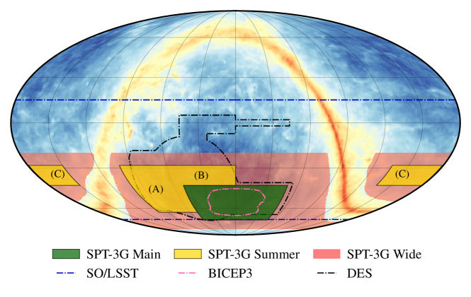
One of the primary science goals of SPT-3G is to create a template of the gravitational-lensing-induced B modes in the patch of sky observed by the BICEP-Keck (BK) family of experiments. This template can be subtracted from the BK data, reducing the primary source of variance in the BK B-mode analysis and potentially improving the sensitivity to primordial gravitational waves by a factor of three. To that end, since 2019, SPT-3G has been used primarily (eight months per year) to observe the 1500 ${\rm deg}^{2}$ SPT-3G Main survey, which overlaps completely with the BICEP3 and BICEP Array sky coverage (see Fig. 1). During the austral summer season (roughly at the beginning of December), when the Sun is above the horizon and gets sufficiently close to the SPT-3G Main survey region, it is picked up by the telescope far sidelobes . Therefore, until sunset, we switch to observing three fields that are safe from sun contamination. These comprise the 2650 ${\rm deg}^{2}$ SPT-3G Summer survey (Fig. 1). We refer to these three fields as Summer-A, Summer-B, and Summer-C.

Even with the added sky coverage of the Summer survey, the constraints on $\Lambda{\rm CDM}$ parameters from SPT-3G data are limited by sample variance. For this reason, we have paused our standard observing strategy for one year to undertake a new survey of all the sky viewable from the South Pole at instrumentally feasible observing elevations and with minimal Galactic foreground contamination. We have empirically determined that, during the winter, we are able to observe with SPT-3G between elevations of roughly $20^{\circ}$ and $80^{\circ}$ (limited by detector linearity at the low end and refrigerator performance on the high end). The intersection of these elevation limits (which, at the South Pole, correspond directly to declination limits) and the Planck GAL080 (Planck Collaboration et al., 2016b) Galactic mask defines our new SPT-3G Wide survey, which totals 6000 ${\rm deg}^{2}$ and is shown in Fig. 1. Observations of the SPT-3G Wide survey commenced in December of 2023 and will continue through the austral winter of 2024. We will refer to the combination of the SPT-3G Main and the SPT-3G Summer surveys as the Ext-4k survey. Similarly, we will refer to the combination of SPT-3G Main, SPT-3G Summer, and SPT-3G Wide surveys as the Ext-10k survey. In Table 1, we summarize the areas and depths for the SPT-3G Main, Summer, and Wide surveys.

The survey footprints for SPT-3G and other surveys are shown in Fig. 1. As is evident from the figure, all the three SPT-3G surveys have an excellent overlap with SO, which will enable a variety of cross-checks to be performed between the two surveys. We list the noise levels and the field centers for the SPT-3G surveys in Table 1. In this work, we produce forecasts both for current noise levels (2019-2023) and for the ones expected from future SPT-3G observations (2024-2026). Besides instrumental noise, our data is also affected by atmospheric noise, which increases towards large angular scales. We model the temperature noise power spectrum as

N_{\ell}=\Delta_{T}^{2}\left[1+\left(\frac{\ell}{\ell_{\text{knee},T}}\right)^{\alpha_{T}}\right]\,,

(1)

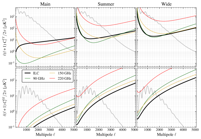
where $\Delta_{T}$ represents the white noise level at a given band in $\mu\mathrm{K}{\rm-arcmin}$ , $\ell_{\text{knee},T}$ and $\alpha_{T}$ are used to parameterize the atmospheric noise. For the SPT-3G Main survey, we adopt the values of $\ell_{\text{knee}}$ and $\alpha$ in Table 2 from previous analyses, but we find that the results of our forecasting are insensitive to the exact values of $\ell_{\text{knee}}$ and $\alpha$ . For the SPT-3G Summer survey, during which the atmospheric opacity and precipitable water vapor levels are higher, we fit real noise data to the model in Eq. 1, and the parameters in the Table 2 are the result of those fits. We also adopt the SPT-3G Summer survey parameters for the SPT-3G Wide survey (which is likely pessimistic for the higher-elevation Wide fields). We extrapolate the white noise levels for deeper integration times. We also fit the noise model parameters for the polarization maps in a similar way. We note that the white noise levels in the polarization maps are roughly $\sqrt{2}\times$ higher than in the temperature maps. In Table 2, we list the $\ell_{\text{knee}}$ and $\alpha$ values adopted for different bands for both temperature and polarization. Finally, we deconvolve the experimental beam window function $B_{\ell}$ from the noise spectra as $N^{\prime}_{\ell}\equiv\dfrac{N_{\ell}}{B_{\ell}^{2}}$ where the beam window function at each frequency is estimated as detailed in Dutcher et al. (2021). We show the model noise spectra in different bands (90 GHz in green, 150 GHz in yellow, and 220 GHz in red) for all the SPT-3G surveys in Fig. 2. These spectra assume integration times of 5 years for the SPT-3G Main survey, 4 years for the SPT-3G Summersurvey, and 1 year for the SPT-3G Wide survey.

3 Forecasting methodology

In this section, we outline the two methods used for calculating the bandpower covariance matrix from which a Fisher matrix for cosmological parameters (Tegmark et al., 1997) can be derived. The first method relies on an analytic approximation (See § 3.2) for the covariance matrix. This approach has been widely adopted in various forecasting studies, and is quite simple and flexible. Our second method employs MUSE (see § 3.3), which is one of the analysis pipelines developed for SPT-3G data. MUSE is more accurate as it readily incorporates non-ideal factors such as covariance between multipoles, covariance between different types of power spectra, and impacts of delensing. Although previous works (for example, Hotinli et al., 2022; Trendafilova, 2023), suggest that these factors may not significantly alter our forecasts, adopting both these methods improves the robustness and reliability of our forecasts. We also describe the method we use to combine Planck data with SPT-3G. We begin with a brief description of how we optimally combine data from multiple frequency bands.

3.1 Linear Combination of Frequency Bands

We combine data from multiple frequency bands listed in Table 1 using a scale-dependent linear combination (LC) technique (Cardoso et al., 2008; Planck Collaboration et al., 2014). In harmonic space denoted by subscript $\ell$ , this corresponds to

S_{\ell m}=\sum_{i=1}^{N_{\mathrm{bands}}}w_{\ell}^{i}M_{\ell m}^{i}\,,

(2)

where $S$ is the desired sky signal (in our case the CMB), $\mathbf{w}_{\ell}$ is the weight, $\mathbf{M}_{\ell m}$ is the spherical harmonic transform of the input map, and the subscript $i$ runs over all the frequency bands. The multipole-dependent weights $\mathbf{w}_{\ell}$ are tuned in order to minimize the overall variance from noise and foregrounds. They are derived as

\mathbf{w}_{\ell}=\frac{\mathbf{C}_{\mathrm{\ell}}^{-1}\mathbf{A_{s}}}{\mathbf{A_{s}}^{\dagger}\mathbf{C}_{\mathrm{\ell}}^{-1}\mathbf{A_{s}}}\,.

(3)

Here $\mathbf{C}_{\mathrm{\ell}}$ is a $N_{\mathrm{bands}}\times N_{\mathrm{bands}}$ matrix containing the covariance of noise and foregrounds across different frequencies at a given multipole $\ell$ ; $\mathbf{A_{s}}=[1\ 1\ ..\ 1]$ is the frequency response of the CMB in different bands and is a $N_{\mathrm{bands}}\times 1$ vector. We model the foreground contribution using results from Reichardt et al. (2021) and the noise modeling is described in § 2.1.

In Fig. 2, we show the LC residuals for all three SPT-3G surveys as the thick black solid curve. The top and bottom panels in the figure are for CMB temperature ( $TT$ ) and polarization ( $EE$ ) power spectra, denoted as gray curves. In the absence of foregrounds, the LC residuals simply correspond to the inverse variance combination of noise from different frequency bands, which is almost true for $EE$ (bottom panels).

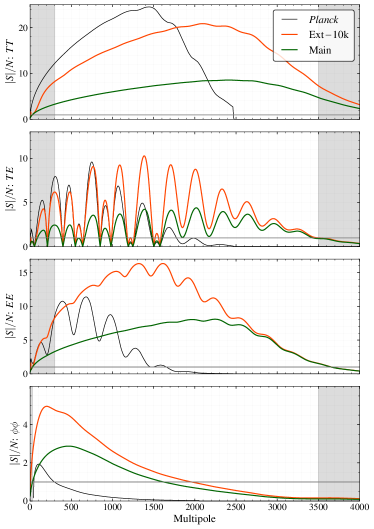
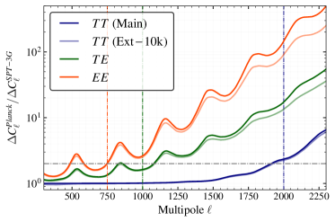
In Fig. 3, we present signal-to-noise ( $S/N$ ) per multipole for $TT/EE/TE/\phi\phi$ spectra for SPT-3G Main (green) and Ext-10k (orange) surveys along with Planck (black). The power spectrum errors were calculated using the analytical formula (see Eq.5) (Knox, 1995; Jungman et al., 1996; Zaldarriaga et al., 1997). Planck has a higher $S/N$ on large scales because of the larger sky coverage. However, the $S/N$ s of SPT-3G Main and Ext-10k surveys are much higher than Planck on small scales. In particular, the $S/N$ s for the Ext-10k survey will surpass Planck beyond $\ell=$ 1800, 800, and 450 for $TT$ , $TE$ , and $EE$ respectively. For $\phi\phi$ , the $S/N$ are better than Planck on all scales. As a result, we can expect significant improvement on cosmological parameters that control structure formation and that are sensitive to the damping tail from SPT-3G compared to Planck as we show later in this work.

3.2 Analytic method

Given a set of power spectra of the lensed CMB and the lensing potential, $X,Y\in[TT,EE,TE,\phi\phi]$ , the Fisher matrix is given by,

\mathcal{F}_{ij}=\sum_{X,Y}\sum_{\ell}\dfrac{\partial C_{\ell}^{X}}{\partial\theta_{i}}\cdot\left(\Sigma_{\ell}^{-1}\right)_{XY}\cdot\dfrac{\partial C_{\ell}^{Y}}{\partial\theta_{j}},

(4)

where $\theta$ s correspond to the cosmological parameters being constrained. The partial derivatives of the spectra with respect to the parameters $\theta$ , denoted as $\partial C_{\ell}/\partial\theta_{j}$ , are obtained using the finite difference method. $\Sigma_{\ell}$ is the covariance of the power spectra, given by Eq.(5) {widetext}

\displaystyle\Sigma_{\ell}=\dfrac{2}{\left(2\ell+1\right)f_{\rm sky}}\begin{pmatrix}(\tilde{C}_{\ell}^{TT})^{2}&(C_{\ell}^{TE})^{2}&\tilde{C}_{\ell}^{TT}C_{\ell}^{TE}&(C_{\ell}^{T\phi})^{2}\\ (C_{\ell}^{TE})^{2}&(\tilde{C}_{\ell}^{EE})^{2}&\tilde{C}_{\ell}^{EE}C_{\ell}^{TE}&(C_{\ell}^{E\phi})^{2}\\ \tilde{C}_{\ell}^{TT}C_{\ell}^{TE}&\tilde{C}_{\ell}^{EE}C_{\ell}^{TE}&\frac{1}{2}\left[(C_{\ell}^{TE})^{2}+\tilde{C}_{\ell}^{TT}\tilde{C}_{\ell}^{EE}\right]&C_{\ell}^{T\phi}C_{\ell}^{E\phi}\\ (C_{\ell}^{T\phi})^{2}&(C_{\ell}^{E\phi})^{2}&C_{\ell}^{T\phi}C_{\ell}^{E\phi}&(\tilde{C}_{\ell}^{\phi\phi})^{2}\end{pmatrix},

(5)

where $f_{\textrm{sky}}$ is the fraction of the sky for the survey under consideration and

\tilde{C}_{\ell}^{X}=C_{\ell}^{X}+N_{\ell}^{X},

(6)

$X=\{TT,EE,\phi\phi\}$ . $N_{\ell}^{TT}$ and $N_{\ell}^{EE}$ are the residual noise and foreground power after combining data from all the bands using the LC method. $N_{\ell}^{\phi\phi}$ is the lensing reconstruction noise derived using Quadratic Lensing Estimator (Hu & Okamoto, 2002). In Table 3 we list the fiducial values of the cosmological parameters at which the Fisher matrix is evaluated and associated priors.

Table 3: Fiducial values of the parameters and priors used in this work. All the applied priors are Gaussian with the widths given below in the table.

Parameter	Fiducial	Prior
$\Lambda{\rm CDM}$ parameters:
Amplitude of scalar	3.044	-
fluctuations ${\rm ln}(10^{10}A_{s})$	3.044
Dark matter density $\Omega_{c}h^{2}$	0.1200
Baryon density $\Omega_{b}h^{2}$	0.02237
Scalar spectral index $n_{s}$	0.9649
Hubble parameter $h$	0.6732
Reionization optical depth $\tau_{\rm re}$	0.0544	0.007
Extensions:
Sum of neutrino masses $\sum m_{\nu}$	0.06 eV	-
Number of relativistic species $N_{\mathrm{eff}}$	3.044
Running of the spectral index $n_{\rm run}$	0
Spatial curvature $\Omega_{k}$	0
Equation of state of dark energy $w_{0}$	-1
Helium abundance $Y_{P}$ ^{${}^{\dagger}$}^{${}^{\dagger}$}footnotemark:	0.245

^†^†footnotetext: Set from BBN (Big Bang nucleosynthesis) consistency when

Y_{P}

is not included in the extension.

We calculate the Fisher matrix for each of the SPT-3G surveys given in Table 1 and combine them to obtain the final SPT-3G Fisher matrices as

$\displaystyle\mathcal{F}_{\rm Summer}$	$\displaystyle=\mathcal{F}_{\rm Summer-A}+\mathcal{F}_{\rm Summer-B}+\mathcal{F}_{\rm Summer-C}$
$\displaystyle\mathcal{F}_{\rm Ext-4k}$	$\displaystyle=\mathcal{F}_{\rm Main}+\mathcal{F}_{\rm Summer}$
$\displaystyle\mathcal{F}_{\rm Ext-10k}$	$\displaystyle=\mathcal{F}_{\rm Main}+\mathcal{F}_{\rm Summer}+\mathcal{F}_{\rm Wide}\,.$	(7)

The parameter covariance matrices are then obtained by inverting the Fisher matrix. We fix the $\ell$ ranges for all the SPT-3G surveys to the following for the Fisher matrix calculation: $300\leq\ell\leq 3500$ for $TT/TE$ ; $300\leq\ell\leq 4000$ for $EE$ ; and $30\leq L\leq 3500$ for $\phi\phi$ . For lensing reconstruction, we use $300\leq\ell\leq 3500$ for T and $300\leq\ell\leq 4000$ for P. We ignore $\ell>3500$ in $TT/TE$ because of the difficulties in modeling the extragalactic foreground signals in the temperature data. We have checked the correlations between the SPT-3G Main and the contiguous SPT-3G Summer surveys and we have found that they are negligible. This is due to the fact that we do not include the large-scale modes $\ell\leq 300$ . Since the extragalactic foregrounds are largely unpolarized (Datta et al., 2019; Gupta et al., 2019), we can set a higher $\ell_{\rm max}$ for $EE$ . We find that extending $\ell_{\rm max}^{EE}>4000$ results in marginal improvements, indicating those modes are noise dominated, as can be inferred from Fig. 3.

3.3 MUSE

MUSE (Millea & Seljak, 2021) is a general algorithm for approximate marginalization over arbitrary latent parameters which yields Gaussianized, asymptotically unbiased and near-optimal constraints on parameters of interest. In our application of MUSE, the parameters of interest are the unlensed $TT$ , $TE$ , $EE$ , and $\phi\phi$ bandpowers, which are weighted averages of the respective power spectra across defined multipole bins. These bandpowers depend on the latent parameters, which are the pixel values of the lensing map and the unlensed CMB field maps.

As previously demonstrated by Millea et al. (2021) using SPTpol data, the standard Quadratic Lensing Estimator is sub-optimal for lensing reconstruction at noise levels below $\Delta_{T}\sim 5\mu\mathrm{K}{\rm-arcmin}$ (Hirata & Seljak, 2003a, b) and hence, using MUSE has an advantage in terms of the lensing reconstruction. Another advantage of MUSE is that it performs optimal delensing on the lensed CMB maps and produces estimates of the unlensed power spectra, lensing potential power spectra and their joint covariance. This covariance naturally includes lensing-induced correlations between different bandpowers ( $\ell-\ell^{\prime}$ ); and also between delensed CMB $TT/EE/TE$ and lensing $\phi\phi$ spectra (Peloton et al., 2017; Trendafilova, 2023).

Despite the above advantages, we do not expect a significant improvement in the constraints from using MUSE over QE methods. This is because the lensing bandpower errors are dominated by sample variance over the angular scales for which MUSE reduces $\phi$ map noise, and the lensing-induced correlations are not important for the current noise levels. Moreover, the optimality of MUSE is non-negligibly better only for the SPT-3G Main survey, and not for the others given their higher noise levels (see Table 1).

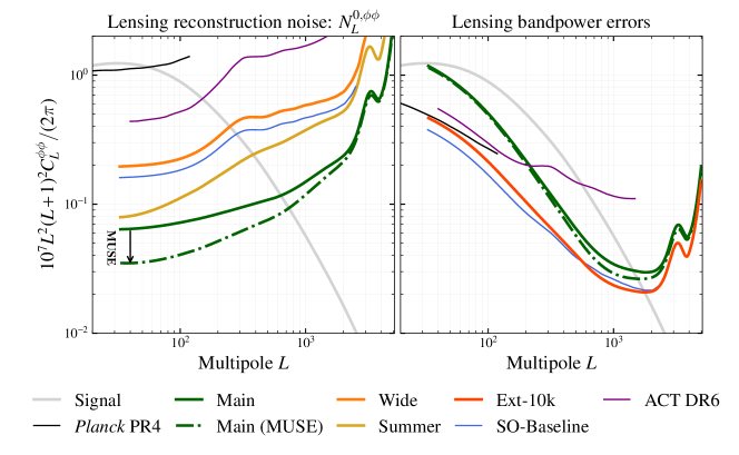
The optimality of the MUSE estimates is useful for other purposes like delensing the lensing-induced B-modes and cross correlations, at least for the SPT-3G Main survey with its low noise levels (see Table 1). We demonstrate this in Fig. 4 which shows the lensing reconstruction noise $N_{L}^{(0,\phi\phi)}$ for different surveys. For the SPT-3G Main survey shown in green, the lensing reconstruction noise goes down by roughly $\times 2.5\ (\times 1.9)$ for polarization-only (including temperature information) lensing estimators when we replace QE (solid) with MUSE (dash-dotted). As mentioned above, the difference between QE and MUSE is negligible for other surveys and hence, not shown.

In MUSE, we express the lensing and unlensed CMB power spectra as scaled versions of the fiducial power spectra, which, for our purposes, are based on the Planck 2015 spectra (Planck Collaboration et al., 2016b). This is given by

C_{\ell}=A_{\ell}C_{\ell}^{\text{fid}}\,,

(8)

where $C_{\ell}^{\text{fid}}$ represents the fiducial power spectrum from the Planck 2015 data, and $A_{\ell}$ is the scaling factor applied to this fiducial spectrum. Here, $C_{\ell}$ is used as a general notation that encompasses all types of power spectra, including unlensed $TT/TE/EE$ and $\phi\phi$ .

In our application of MUSE, we do not estimate the power at each individual multipole but instead bandpower parameters, $A_{b}$ , that each scale a fiducial power spectrum across a band of width $\Delta\ell=100$ . As a result, MUSE produces a covariance matrix of these scaling coefficients $\Sigma_{A_{b}}\equiv\left<A_{b}A_{b}^{*}\right>$ . The $A_{b}$ can be understood as the binned version of $A_{\ell}$ .

As described below, this covariance is subsequently utilized to construct the cosmological parameter-Fisher matrix, from which we derive the constraints on parameters. We provide more details about MUSE in the appendices. Specifically, we describe the derivation of the MUSE covariance matrix in Appendix A, the simulations used for estimating the covariance matrix in Appendix A.1, and the lensing reconstruction noise in Appendix A.2.

The standard Fisher formula described in the previous section Eq.(4) can be adapted to incorporate the MUSE covariance matrix $\Sigma_{A_{b}}$ . Let the covariance matrix of the power spectra be represented by $\Sigma_{C_{\ell}}$ and the covariance matrix of the amplitudes be represented by $\Sigma_{A_{\ell}}$ , then the Fisher matrix can be written as,

$\displaystyle\mathcal{F}_{ij}$	$\displaystyle=\sum_{XY}\sum_{\ell\ell^{\prime}}\dfrac{\partial C_{\ell}^{X}}{\partial\theta_{i}}\left(\Sigma_{C_{\ell}}^{-1}\right)_{XY}^{\ell\ell^{\prime}}\dfrac{\partial C_{\ell^{\prime}}^{Y}}{\partial\theta_{j}}$	(9)
	$\displaystyle=\frac{1}{C^{\text{fid}}_{\ell}}\frac{\partial C_{\ell}}{\partial\theta_{i}}\cdot\left(\Sigma_{A_{\ell}}^{-1}\right)\cdot\frac{1}{C^{\text{fid}}_{\ell}}\frac{\partial C_{\ell}}{\partial\theta_{j}}$	(10)
	$\displaystyle\approx\dfrac{\partial A_{b}}{\partial\theta_{i}}\cdot\left(\Sigma_{A_{b}}^{-1}\right)\cdot\dfrac{\partial A_{b}}{\partial\theta_{j}}.$	(11)

For ease of notation, we drop the summation symbols and transition to using matrix products in the second line. In the last line we assume that the Fisher matrix is approximately equivalent to its binned version. We obtain the derivatives of $A_{b}$ with respect to the cosmological parameters via a minimum-variance binning of $\partial C_{\ell}/\partial\theta$ given by

\dfrac{\partial A_{b}}{\partial\theta}=\dfrac{1}{\sum_{\ell\in b}\dfrac{1}{\sigma_{A_{\ell}}^{2}}}\sum_{\ell\in b}\dfrac{1}{\sigma_{A_{\ell}}^{2}}\dfrac{\partial C_{\ell}/\partial\theta}{C_{\ell}^{\text{fid}}}\,,

(12)

where we use an analytic ansatz for the weighting function $\sigma_{A_{\ell}}^{2}$ . For $X\in[TT,EE,\phi\phi]$ this is given by

\sigma_{A_{\ell}^{X}}^{2}=\frac{\sigma^{2}_{C_{\ell}^{X}}}{(C_{\ell}^{X,\text{fid}})^{2}}\equiv\frac{2}{2\ell+1}\frac{(C_{\ell}^{X}+N_{\ell}^{X})^{2}}{(C_{\ell}^{X,\text{fid}})^{2}}

(13)

and for $TE$ it is

\sigma_{A_{\ell}^{TE}}^{2}=\frac{1}{2\ell+1}\frac{(C_{\ell}^{TE})^{2}+(C_{\ell}^{TT}+N_{\ell}^{TT})(C_{\ell}^{EE}+N_{\ell}^{EE})}{(C_{\ell}^{TE,\text{fid}})^{2}}.

(14)

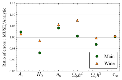
In Fig. 5, we show the ratio of parameter constraints obtained from MUSE and the analytic covariance for SPT-3G Main (green) and the SPT-3G Wide (orange) surveys. We find that these methods are consistent with each other within a 10% margin, which we deem sufficient to satisfy our validation criteria.

There are a number of reasons to expect these errors to differ to some degree, which we already brought up when describing the advantages of MUSE. Another reason is that the analytic results are not binned, but we found that for both the Wide and Main surveys, binning to $\Delta\ell=100$ only leads to at most 2% degradation in constraints. The largest difference is the 8% tighter constraint on $\Omega_{b}h^{2}$ from the analytic forecast for the SPT-3G Wide survey. This is because the analytic estimate does not include the $\ell$ -by- $\ell$ lensing-induced correlations among different CMB multipoles, and that can lead to overly-optimistic constraints. By artificially removing off-diagonal elements from the MUSE covariance matrix²²2Specifically we did this by inverting it, removing the off-diagonals, and inverting back, we were able to largely reproduce this reduced analytic error for both $\Omega_{b}h^{2}$ and $n_{s}$ .

3.4 Combining with Planck data

Comparison of the SPT-only $\Lambda{\rm CDM}$ constraints with those from Planck, as we will see, will enable a powerful test of the $\Lambda{\rm CDM}$ model. If these tests are consistent with $\Lambda{\rm CDM}$ then we will be interested in using the combined SPT-3G+Planck data to estimate $\Lambda{\rm CDM}$ parameters, as Planck provides complementary information on large angular scales. Consistent or not, we will also be interested in using the combined data to constrain $\Lambda{\rm CDM}$ extensions. Hence, we report the expected constraints from the combined datasets under the assumption of $\Lambda{\rm CDM}$ as well as under the assumption of various extensions.

The standard approach to obtain this combination is to add the Fisher matrices from SPT-3G and Planck similar to Eq.(7) as

\displaystyle\mathcal{F}_{{\rm SPT}+{\it Planck}}

\displaystyle=\mathcal{F}_{\rm\widehat{SPT}}+\mathcal{F}_{\widehat{{\it Planck}}},

(15)

where $\mathcal{F}_{\rm\widehat{SPT}}$ is the modified SPT-3G Fisher matrix obtained by taking the inverse variance combination of SPT-3G and Planck noise in the field under consideration; and $\mathcal{F}_{\widehat{{\it Planck}}}$ is the modified Planck Fisher matrix after scaling to remove the overlapping sky region between SPT-3G and Planck. For example, if $f_{\mathrm{sky}}=1$ for $\mathcal{F}_{{\it Planck}}$ , then for $\mathcal{F}_{\widehat{{\it Planck}}}$ , we use $f_{\mathrm{sky}}=1-f_{\mathrm{sky}}^{\rm SPT}$ .

However, obtaining Eq.(15) is non-trivial as it requires us to know the sky fraction used by Planck, which varies for different bands and power spectra (Planck Collaboration et al., 2020). Instead, we follow a different approach which involves two steps: First, we derive the Planck Fisher matrix directly from the publicly available Planck PR3 chains (Planck Collaboration et al., 2020); second, when combining the above Planck Fisher matrix with SPT-3G, we modify the SPT-3G Fisher matrix by removing the large-scale modes from it, to avoid double counting information in the overlapping region.

We use BASE_PLIKHM_TTTEEE_lowL_lowE_lensing³³3Planck chains are downloaded from https://wiki.cosmos.esa.int/planck-legacy-archive/index.php/Cosmological_Parameters chains for the first step unless specified otherwise. These chains, which contain samples from the probability distribution of cosmological parameters, are used to construct a parameter covariance matrix. By inverting this covariance matrix, we obtain the Planck Fisher matrix. For the second step, we restrict the information we use from SPT power spectra to multipoles above some $\ell_{\rm min}$ or $L_{\rm min}$ threshold, set by the approximate multipole at which the $S/N$ for Planck is $\times 2$ lower than that for SPT in the same patch. We find that the choice of $\ell_{min}$ does not change significantly for different SPT-3G surveys. As can be seen from Fig. 6, which shows the ratio of Planck $TT$ , $TE$ , and $EE$ power spectrum uncertainties to those projected for SPT-3G, this threshold is roughly 2000, 1000, and 750 for $TT$ , $TE$ , and $EE$ respectively, and we adopt these values for the joint forecasting. For lensing power spectra, we set $L_{\rm min}=30$ (the same as our fiducial setting) because Planck’s lensing $S/N$ is much lower than SPT on all scales, as can be seen from Fig. 3. However, we find our forecasts to be insensitive to the choice of $L_{\rm min}$ . For example, with $L_{\rm min}=400$ for SPT, our constraints only weaken by $\lesssim 5\%$ .

We validate this approach of using $\ell_{\rm min}$ cuts rather than the $f_{\mathrm{sky}}$ scaling in Eq.(15) by creating a toy model for a Planck-like Fisher matrix with $f_{\mathrm{sky}}=0.5$ . For this toy model, we use the following multipole ranges: $\ell\in[2,2000],\ [30,2000],\ [30,2000]$ respectively for $TT$ , $TE$ , and $EE$ and $L\in[30,400]$ for $\phi\phi$ . Next, we compare the Fisher forecasts from Eq.(15) and the $\ell_{\rm min}$ -cut approach discussed above. We find the results from the $\ell_{\rm min}$ cut approach to be $\lesssim 8\%$ worse than the traditional method. Given that the two methods agree well and given that our $\ell_{\rm min}$ -cut-based forecasts are slightly on the conservative side, we choose to use this approach for the rest of this work.

4 Results

In this section, we begin by presenting our forecasts on cosmological parameters using all three SPT-3G surveys, assuming the 6-parameter $\Lambda{\rm CDM}$ model. Subsequently, we project the extent to which combined SPT-3G and Planck data can constrain both single- and double-parameter extensions to the $\Lambda{\rm CDM}$ model. We also qualitatively investigate how well SPT-3G data can differentiate between $\Lambda{\rm CDM}$ and alternative models that have been proposed in the literature to address current cosmological tensions (for example, Cyr-Racine et al., 2022; Schöneberg et al., 2022; Meiers et al., 2023; Hughes et al., 2023; Khalife et al., 2023; Schöneberg et al., 2022). The models we consider are fully consistent with current CMB and lensing power spectra measurements but make different predictions, from those of $\Lambda{\rm CDM}$ , for signals that can be measured well by SPT-3G.

4.1 Forecasts of constraints on $\Lambda{\rm CDM}$ parameters

We start first with forecasts of constraints on the six parameters of the $\Lambda{\rm CDM}$ model, namely baryon density $\Omega_{b}h^{2}$ , cold dark matter density $\Omega_{c}h^{2}$ , Hubble constant $H_{0}$ , optical depth to reionization $\tau_{\rm re}$ , amplitude (defined at the pivot scale $k_{0}=0.05$ Mpc^-1) and spectral index of scalar fluctuations, $A_{s}$ and $n_{s}$ . For these constraints we fix the neutrino mass to the minimal value of $0.06$ eV. We also include a prior on $\sigma(\tau_{\rm re})=0.007$ from Planck (Planck Collaboration et al., 2020). We use the MUSE approach as described in § 3.3 to derive these constraints, and remind the reader that there is agreement between MUSE and the traditional analytic approach to better than 10%, as shown in Fig. 5.

As we will see below, SPT-3G can produce constraints on $\Lambda{\rm CDM}$ parameters that are tighter than those we have from Planck. Since these constraints are obtained from largely different signals than those from Planck, they provide a robust consistency test for the $\Lambda{\rm CDM}$ model. As mentioned earlier in § 3.4, we also present $\Lambda{\rm CDM}$ forecasts by combining SPT-3G and Planck.

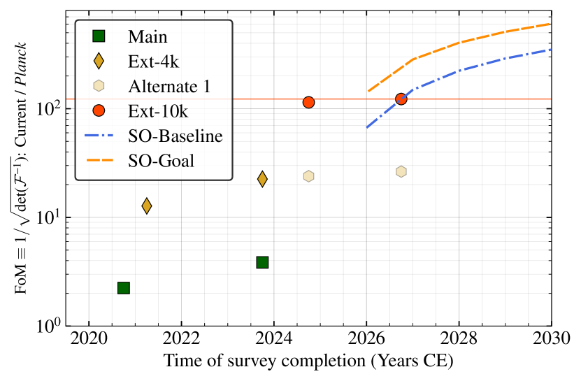
In Fig. 7, we present the projected Figure of Merit (FoM), which is inversely proportional to the volume of allowed 6-dimensional $\Lambda{\rm CDM}$ parameter space. It is calculated as

{\rm FoM}=\sqrt{1/{\rm det}(\mathcal{F}^{-1})}

(16)

for different SPT-3G surveys (SPT-3G Main in green, Ext-4k in yellow, and Ext-10k in orange-red) along with SO (blue). The FoM is inversely proportional to the 6-dimensional volume of the 68% confidence region.⁴⁴4In our Gaussian approximation, this proportionality holds independent of whether it is 68%, 95% or any other such threshold for defining the confidence region We plot it divided by the FoM for Planck.

As is evident from the figure, SPT-3G surveys significantly increase the FoM relative to that from Planck. From just the first two years (2019-2020) of SPT-3G Main survey data, the FoM increases by $\times 2.5$ over Planck, and that jumps to $\times 13$ with the addition of the first two years of SPT-3G Summer data. Both of these are further improved by roughly $\times 1.7$ with the inclusion of SPT-3G Main and SPT-3G Summer survey data through 2023.

The figure also demonstrates the benefit of expanding sky coverage rather than continuing to go deeper on the SPT-3G Main survey patch. One can see this from the minimal improvement to Ext-4k ( $\times 1.1$ ) that we anticipate if we continue with the SPT-3G Main survey patch observations for the 2024 winter, indicated by the semi-transparent yellow circle. On the other hand, switching to the SPT-3G Wide observations in the 2024 season improves the constraining power by $\times 5$ compared to Ext-4k and by $\times 130$ compared to Planck.

Were we to observe the SPT-3G Wide patch for one more year we would not notice a significant increase in the FoM. Instead of doing this we plan to switch back to the SPT-3G Main survey during the 2025 and 2026 winter seasons. Further noise reduction in the SPT-3G Main survey will not increase the FoM much, as can be seen in Fig. 7, but will significantly improve the measurements of the secondary CMB anisotropies including lensing, which will further improve the subtraction of lensed B-modes and hence, the search for B-modes from primordial gravitational waves (Ade et al., 2021).

Table 4: Forecasted

1\sigma

errors on

\Lambda{\rm CDM}

parameters for various survey regions using SPT data. The numbers in the parentheses correspond to the constraints obtained when SPT-3G is combined with Planck. Note that when SPT-3G is combined with Planck, we remove information below

\ell_{\rm min}=2000,1000,750,30

for

TT,TE,EE

and

\phi\phi

power spectra respectively from SPT-3G, to avoid double counting information.

Parameter	SPT-3G Main	SPT-3G Summer	SPT-3G Wide	Ext-4k	Ext-10k
$A_{s}$ [ $10^{-11}$ ]	2.79 (2.47)	2.66 (2.50)	2.54 (2.42)	2.53 (2.38)	2.35 (2.29)
$H_{0}[{\rm km/s/Mpc}]$ [ $10^{-1}$ ]	3.28 (3.16)	3.91 (3.47)	3.49 (3.26)	3.03 (2.95)	2.78 (2.78)
$n_{s}$ [ $10^{-3}$ ]	7.23 (3.14)	6.12 (3.16)	5.10 (3.03)	4.76 (3.00)	3.66 (2.83)
$\Omega_{b}h^{2}$ [ $10^{-5}$ ]	12.9 (7.87)	14.9 (8.68)	11.9 (7.66)	9.5 (6.7)	7.37 (5.67)
$\Omega_{c}h^{2}$ [ $10^{-4}$ ]	8.86 (7.71)	9.84 (8.34)	8.92 (7.97)	8.07 (7.39)	7.36 (7.10)
$\tau_{\rm re}$ [ $10^{-3}$ ]	6.85 (6.64)	6.78 (6.65)	6.59 (6.47)	6.63 (6.42)	6.28 (6.19)

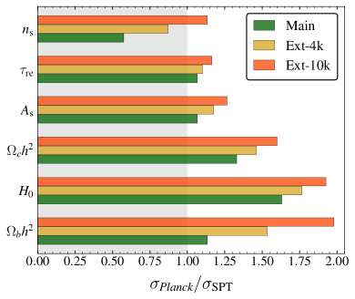
In Table 4 we list our forecasts of $\Lambda{\rm CDM}$ parameter errors for different SPT-3G datasets. We also present them in Fig. 8, where the bars show the ratios of the values of $\sigma(\theta)$ from Planck to those from SPT.

Let us begin by noting two things relevant for interpretation of our $A_{s}$ and $\tau_{\rm re}$ results. First, the calibration of SPT-3G maps relies on data from Planck (Dutcher et al., 2021), and, consequently, SPT-3G constraints on the normalization parameter $A_{s}$ are not entirely independent of Planck. Second, for SPT-only constraints in this work, we include a Planck-like prior on the optical depth, $\sigma(\tau_{\rm re})=0.007$ , since $\tau_{\rm re}$ is primarily constrained by the large-scale $\ell\lesssim 10$ reionization bump in $EE/TE$ , not accessible by SPT. All the $\tau_{\rm re}$ constraints are dominated by this prior. These two points are not unrelated since the combination $A_{s}\ e^{-2\tau_{\rm re}}$ is very tightly constrained by CMB data at $\ell>20$ , so improvements in $\tau_{\rm re}$ determination translate into improvements in $A_{s}$ determination, and vice versa. The small improvements that we do see in $\tau_{\rm re}$ are due to the dependence of the amplitude of gravitational lensing on $A_{s}$ , an amplitude unaffected by $\tau_{\rm re}$ .

Focusing on the other four parameters, we find that the SPT-only constraints are generally comparable to, or better than, those obtained from Planck alone, for each of our three SPT-3G survey combinations. For the case of Ext-10k, the improvements in $H_{0}$ and $\Omega_{b}h^{2}$ are nearly a factor of 2, and for $\Omega_{c}h^{2}$ they are just more than a factor of 1.5. For $n_{s}$ , the relative errors from SPT-3G Main survey and Ext-4k survey are larger compared to those from Planck due to Planck’s significantly broader multipole range. Nonetheless, the Ext-10k survey still manages to achieve slightly tighter constraints on $n_{s}$ than what we have from Planck.

4.1.1 Comparison with SO

In Fig. 7, we also show the expected constraining power from the Simons Observatory for two configurations: SO-Baseline (blue dash-dotted) and SO-Goal (orange dash-dotted), based on the noise levels in Simons Observatory Collaboration (2019). We use the original SO noise model code⁵⁵5https://github.com/simonsobs/so_noise_models to get the noise curves but use the same multipole ranges described in § 3.2 for forecasting. As a check, we compare the constraints that we get from our forecasts for SO against what is reported in Simons Observatory Collaboration (2019) but note that we do not include Planck unlike SO’s original forecasts.

Comparing our forecasts for SO to Table 3 of Simons Observatory Collaboration (2019), our forecasts are slightly better for $H_{0}$ and $\Omega_{c}h^{2}$ but they agree within 10%. For $n_{s}$ and $\Omega_{b}h^{2}$ , we obtain 15-35% worse constraints, which is presumably because we do not add the large-scale information from Planck. On the other hand, we obtain roughly 35% (20%) better constraints on $A_{s}$ ( $\tau_{\rm re}$ ). When we increase the prior uncertainty on optical depth to $\sigma(\tau_{\rm re})=0.009$ to match SO’s forecasting code (see caption of Table 3 in Simons Observatory Collaboration 2019), our results on $A_{s}$ and $\tau_{\rm re}$ match the numbers quoted in Simons Observatory Collaboration (2019). Switching to SO-Goal configuration reduces the errors on all parameters by 5% except for $\Omega_{c}h^{2}$ where the constraining power improves by 15%.

We also note from Fig. 7, the constraining power of the SPT-3G Ext-10k survey for $\Lambda{\rm CDM}$ parameters will be roughly similar to the first two years of SO-Baseline. Such similar levels of constraining power between SPT and SO along with significant sky overlap (see Fig. 1) will allow for comparisons of the two datasets at both the power spectrum and map level (such as the ACT-Planck and SPT-Planck comparisons shown in Louis et al. 2014 and Hou et al. 2018) which will provide useful opportunities for identifying and/or limiting systematic errors in individual datasets.

4.1.2 Real-world effects

In this section, we examine how our forecasts change as we vary our baseline modeling assumptions, and introduce additional non-ideal aspects into our model of the data on which the forecasts are based. We modify our noise curves to account for filtering effects and to include a higher level of complexity in the noise due to the correlated atmospheric signal on large scales in the temperature data. We also investigate the degradation in constraints that could come from galactic foregrounds. We also check the impact of including uncertainties in the calibration of our temperature and polarization maps. As detailed below, we find the degradation of parameter errors relative to the baseline case, from all of these effects, is $\lesssim 10\%$ . Finally, we build further confidence in our forecasts by comparing them to constraints from an ongoing MUSE analysis of the two-year SPT-3G Main data.

Atmospheric noise

The first thing we examine is the impact of the filtering applied to the detector time-ordered data (TOD) before it is processed into maps. To avoid excess noise in the scan direction in the resulting maps, primarily as a result of the large-scale atmospheric noise, we apply filters to remove the long-timescale information from the detector TOD. While this improves the quality of the maps, it results in a reduction of data volume that increases the final power spectrum errors by a factor equivalent to raising map noise levels by roughly 10%. We test the impact of this by increasing the white noise levels in Table 1 by 10%. We found that this results in changes to the parameter constraints at the $\leq 1\%$ level. Secondly, since SPT-3G uses multichroic detectors that can simultaneously observe in multiple frequencies, the large-scale atmospheric noise is expected to be correlated between bands. From the 2019-20 dataset, we estimate the correlation at the largest scales to be $\sim 90\%$ between the 150 and 220 GHz bands, and around $70\%$ between the 90 and 150 GHz bands as well as between the 90 and 220 GHz bands. This degree of correlation diminishes as we move to small scales. To take this into account, we set the cross-frequency noise to be correlated across bands and rerun the LC step to get the residuals. This correlated noise, in fact, reduces the large-scale LC residuals slightly. When we propagate these to parameter constraints, we find changes to the parameter constraints at the $\leq 1\%$ level, indicating that our forecasts are robust to these details about the noise spectra.

Galactic foregrounds and mask

Given that the SPT-3G Wide survey extends close to the plane of the galaxy (see Fig. 1), it is crucial to understand the impact of galactic foregrounds on the parameter constraints. To assess this, we make use of the PySM simulations (Thorne et al., 2017) of galactic foregrounds and the galactic foreground masks (GAL070, GAL080, GAL090) produced by the Planck collaboration (Planck Collaboration et al., 2016b). The names of the above masks correspond to the sky retained after masking the galactic plane. For instance, GAL090 masks 10% of the region with a high level of foregrounds close to the galactic plane while GAL070 removes 30% of the sky and is the most conservative amongst the three.

We use these masks and calculate the level of galactic dust and synchrotron signals in PySM simulations in the following regions: Case (A) GAL080-GAL070; Case (B) GAL090-GAL070; and Case (C) GAL090-GAL080. The three cases correspond to the differences between the respective masks; for instance, GAL080-GAL070 represents the sky area included in mask GAL080 but excluded in GAL070. As expected, we find the galactic foreground in Case (C) to be the highest followed by Cases (B) and (A).

We perform a conservative test by assuming that the galactic foreground levels across the entire SPT-3G Wide survey match one of these three cases. With this assumption, we derive the LC residuals and the subsequent impact on the parameter constraints. Even for Case (C), where the galactic foregrounds are the highest, we find the constraints degrade by only $8\%$ . This is not surprising given that the galactic foregrounds are mostly important on the largest scales and the constraining power of SPT-3G is predominately driven by the high- $\ell$ region.

In the preceding sections, we mentioned that the observing strategy to minimize galactic foreground contamination in the SPT-3G Wide involves observing within the confines of the Planck GAL080 mask, which corresponds to roughly $6000\,{\rm deg}^{2}$ of sky coverage. In the scenario where we might need to adopt a more conservative Planck GAL070 mask, we found that this would lead to a modest degradation in parameter constraints, at 4-5%. While we do not address potential biases due to mismodeling of the galactic foregrounds, we remain confident that any such biases would be minimal, given that the levels of galactic foregrounds are significantly lower than the CMB power spectra levels at the multipoles relevant to this analysis.

Temperature and polarization calibration

Next, we assess the impact of calibration uncertainty on the temperature and polarization maps by including two absolute calibration parameters, $T_{\rm cal}$ and $P_{\rm cal}$ (as defined in Dutcher et al., 2021), in our forecasts and marginalizing over them. In the case where we do not apply a prior, we find a significant $\times 2$ hit on some of the parameters, which is not surprising since parameters like $A_{s}$ are fully degenerate with the calibration parameters. By comparing SPT-3G Main survey maps from 2019-2020 to Planck maps in that same region, we are able to constrain $T_{\rm cal}$ and $P_{\rm cal}$ to roughly 0.2% and 1%, respectively (where the errors are a combination of statistical uncertainty in the comparison and uncertainties in the Planck calibration). If we adopt these as priors, the resulting degradation in the parameter constraints are $\leq 5\%$ for all parameters. If we loosen the $T_{\rm cal}$ prior to 1%, the degradation increases to $\sim 20\%$ . If we assume either parameter is estimated perfectly and allow for uncertainty in only one calibration parameter, we find the resulting degradation to be negligible, even without any prior, consistent with the results from Galli et al. (2021).

Finally, we replace the covariance matrix for the 2-year SPT-3G Main survey from this work with the one from an ongoing MUSE analysis performed on the real data from the same survey. The latter takes into account certain effects that are present in the real data but not taken into account in our forecasts. These include anisotropic noise, anisotropic filtering, and masking. With this covariance swap, we find that the degradation in the parameter constraints is $\leq 10\%$ .

4.2 Single-parameter extensions to $\Lambda{\rm CDM}$

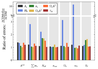
Now we turn our attention towards extensions to the $\Lambda{\rm CDM}$ model. For extensions, we always combine SPT-3G with Planck. We consider 7 different cases by varying the following parameters one at a time along with the 6 $\Lambda{\rm CDM}$ parameters: dark-energy equation of state ( $w_{0}$ ), Helium mass fraction ( $Y_{P}$ ), running of the spectral index ( $n_{\rm run}\equiv{\rm d}n_{s}/{\rm d}\ln k$ ), sum of neutrino masses ( $\sum m_{\nu}$ ), effective number of neutrino species ( $N_{\mathrm{eff}}$ ) and the spatial curvature parameter ( $\Omega_{k}$ ). The forecasted constraints for Ext-10k are reported in Fig. 9. As before, we show the improvement in constraints compared to Planck using the bars. The actual parameter constraints are given in the text boxes. The constraints from other SPT-3G surveys are presented in Table 5 of Appendix B.

We find a significant ( $\times 2-\times 3$ ) reduction of the errors in many of these parameters, namely $\sum m_{\nu}$ , $w_{0}$ , $Y_{P}$ , and $N_{\mathrm{eff}}$ . For other parameters, namely $\Omega_{k}$ , and $n_{\rm run}$ , the improvement is $\times 1.4-\times 1.7$ compared to Planck. Some of these improvements are driven by the inclusion of lensing ( $\Omega_{k},w_{0}$ ) while others come from higher-redshift information in the damping tail of the CMB, whose extraction benefits from wide sky coverage ( $n_{\rm run}$ , $Y_{P}$ , and $N_{\mathrm{eff}}$ ).

We also investigate the degradation in $\Lambda{\rm CDM}$ constraints due to degeneracies with the extension parameters. We present these error degradations in Fig. 10 for Ext-10k+Planck; the full list can be found in Table 6 of Appendix B. As can be inferred from the figure, the constraints on the Hubble constant $H_{0}$ degrade significantly when we free $\theta\in[\sum m_{\nu},N_{\mathrm{eff}},\Omega_{k},w_{0}]$ . Note that these degradations largely disappear with the addition of external datasets that constrain the redshift-distance relationship down to $z\lesssim 0.1$ , namely supernova brightness measurements. This is the reason why these extensions are not viable solutions to the $H_{0}$ tension (Knox & Millea, 2020). The degradation is less severe ( $\sim\times 1.6$ ) for $n_{s},\Omega_{b}h^{2}$ when we vary $\theta\in[N_{\mathrm{eff}},Y_{P}]$ . For the rest, the constraints are robust and the degradation is $\lesssim\times 1.3$ .

In expanding the parameter space from $\Lambda{\rm CDM}$ to $\Lambda{\rm CDM}$ + $w_{0}$ , we notice an unexpected tightening in the constraints for parameters $\Omega_{b}h^{2}$ , $\Omega_{c}h^{2}$ , and $n_{s}$ . We suspect that this arises from our use of a Gaussian approximation for a posterior that is significantly non-Gaussian. The non-Gaussianity is visually evident in the one and two-dimensional marginal posteriors derived from the appropriate Planck chains. With the addition of an $H_{0}$ prior, the range of acceptable $w$ values tightens significantly, reducing the degree of non-Gaussianity, and this anomalous behavior of our forecasts no longer appears.

4.3 Double-parameter extensions to $\Lambda{\rm CDM}$

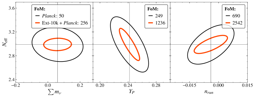
We also explore two-parameter extensions similar to those considered in Planck Collaboration et al. (2020). These are (a) $N_{\mathrm{eff}}$ and $Y_{P}$ , (b) $N_{\mathrm{eff}}$ and $n_{\rm run}$ , and (c) $N_{\mathrm{eff}}$ and $\sum m_{\nu}$ . In Fig. 11, we present the marginalized two-dimensional contours for the above extensions from both Planck (black) and Ext-10k+Planck (orange). The FoM for the two-parameter extensions, calculated similar to Fig. 7, is given in the legend. In most cases, we find an improvement of greater than a factor of 2 relative to Planck alone.

In case (a), we vary the effective number of neutrino species $N_{\mathrm{eff}}$ and the fraction of baryonic mass in helium $Y_{P}$ simultaneously. Such constraints are useful for constraining scenarios in which the value of $N_{\rm eff}$ at big bang nucleosynthesis differs from that at recombination (Millea et al., 2015; Cyburt et al., 2016; Particle Data Group et al., 2020). Since both these parameters affect the damping tail of the CMB, they are partially degenerate and, as expected, the constraints on both parameters degrade by more than $\times 2$ compared to the single-parameter extensions in Fig. 9.

In case (b), we vary $N_{\mathrm{eff}}$ and $n_{\rm run}$ which are also degenerate to some level leading to $\times 1.5$ weaker constraints compared to Fig. 9.

In case (c), we vary $N_{\mathrm{eff}}$ and the sum of neutrino masses $\sum m_{\nu}$ since one can expect some level of correlation between the two (Planck Collaboration et al., 2020). However, this correlation depends on the datasets being considered. In our case, $\sum m_{\nu}$ is primarily constrained by lensing while $N_{\mathrm{eff}}$ constraints are dominated by the small-scale $TT$ , $EE$ , and $TE$ power spectra. Subsequently, the degradation in the constraints on these two parameters is negligible compared to what we obtain for the single-parameter extensions in Fig. 9.

5 Power spectrum predictions from $\Lambda{\rm CDM}$ and alternatives

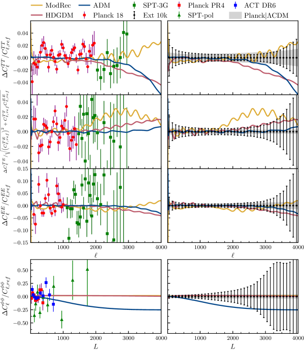
In this section we discuss, in a qualitative manner, prospects for using SPT-3G data to detect departures from $\Lambda{\rm CDM}$ predictions for CMB power spectra conditioned on Planck data. Many alternative models that resolve cosmological tensions, such as the $H_{0}$ and $\sigma_{8}$ tensions, predict power spectra that differ from $\Lambda{\rm CDM}$ predictions at small angular scales, and we use a selection of such models to guide our discussion. In Fig. 12, we present the $\Lambda{\rm CDM}$ predictions for angular power spectra given Planck data, the predictions of alternative models that fit the Planck data well while either having a high $H_{0}$ or a low $\sigma_{8}$ , and the forecasted Ext-10k error bars.

The selected alternative models are (a) a phenomenological model of non-perturbatively modified recombination (ModRec) (Lynch et al. 2024, in preparation); (b) an atomic dark matter (ADM) model arising from a hidden dark sector charged under a U(1) gauge interaction (Hughes et al., 2023); and (c) a model featuring an additional dark fluid with an equation of state parameter that is a free function of redshift, hereafter “high dimensional generalized dark matter” (HDGDM) (Meiers et al., 2023).

We present one set of spectra from each of these models in Fig. 12 as a relative shift $\Delta C_{\ell}^{X}=C_{\ell}^{X}-C_{\ell,{\rm ref}}^{X}$ compared to the reference $\Lambda{\rm CDM}$ mean Planck $C_{\ell,{\rm ref}}^{X}$ , normalized as described in the figure caption. Here $X$ corresponds to one of the primary lensed CMB $TT/EE/TE$ or the lensing $\phi\phi$ power spectra. Each of these spectra are drawn from posterior distributions conditioned on Planck and BAO data, although the HDGDM spectra also includes uncalibrated supernovae data in the fit. It should be noted that the specific BAO datasets used in these constraints differ: please see the appropriate references for details.

The left-hand panels of Fig. 12 show these spectra in relation to existing CMB measurements from Planck, SPTpol (Bianchini et al., 2020), SPT-3G 2018 (Dutcher et al., 2021) and ACT DR6 (Qu et al., 2024). For angular scales that have been probed by multiple experiments, only the most constraining dataset has been plotted. This set of panels highlights that although these models make predictions that differ from $\Lambda{\rm CDM}$ , they are currently not ruled out by the data. To the right, we show the 68% confidence region for angular power spectrum predictions conditioned on Planck data and assuming $\Lambda{\rm CDM}$ , along with forecasted bandpower errors for Ext-10k in black.

The Planck data, along with the assumption of $\Lambda{\rm CDM}$ , make tight predictions for the power spectrum residuals even at angular scales not probed by Planck. This is evident from the righthand panels of Figure 12, where the gray confidence interval extends to no more than about 2% for the $TT$ , $TE$ , and $EE$ power spectra. This range represents the expected region that the power spectra observed by SPT-3G will fall in if measurements continue to be consistent with $\Lambda{\rm CDM}$ . As is evident in these panels, the alternative models presented here exhibit deviations which are larger than this expected range, and larger than the expected precision of SPT-3G. We now discuss each of these models in turn.

The potential role of changes to recombination in alleviating the $H_{0}$ tension has been explored in Chiang & Slosar (2018); Hart & Chluba (2020a); Sekiguchi & Takahashi (2021); Lee et al. (2023); Cyr-Racine et al. (2022). Physical models which have a modified recombination epoch include models with varying fundamental constants (Ade et al., 2015; Hart & Chluba, 2018, 2020b; Sekiguchi & Takahashi, 2021), primordial magnetic fields (Jedamzik & Pogosian, 2020; Galli et al., 2022; Rashkovetskyi et al., 2021), or energy injection from decaying dark matter (Galli et al., 2013; Slatyer & Wu, 2017; Finkbeiner et al., 2012). The ModRec model presented here is an extension of $\Lambda{\rm CDM}$ that allows for a purely phenomenological modification of the ionization fraction as a function of redshift through the epoch of hydrogen recombination, in order to study the role of these changes independently of the details of particular physical models. We note that the different modified ionization fractions predicted by the above physical models can be well approximated within the ModRec model using seven parameters characterizing deviations from the standard recombination scenario.

This additional freedom allows for higher values of $H_{0}$ to provide good fits to the Planck data. The ModRec model accommodates a high value of $H_{0}$ by altering the recombination process, shifting last scattering to higher redshifts and increasing the width of the visibility function. This reduces the comoving size of the sound horizon at recombination, so that the shorter distance to last-scattering associated with a higher $H_{0}$ does not shift the well-determined angular size of the sound horizon. It also impacts the damping scale, an effect ameliorated by the change to the visibility function width.

In Fig. 12 we show predictions within the ModRec model for a set of parameters which fit Planck and eBOSS BAO data at least as well as a $\Lambda{\rm CDM}$ best-fit, while having $H_{0}=70.48$ km/s/Mpc. To maintain the fit with Planck data, residuals with respect to the fiducial cosmology get shifted to higher multipoles, which, while unprobed by Planck, are expected to be measured with high SNR by SPT-3G. We see that SPT-3G has clear potential to rule out such a model, particularly through measurements of the $TE$ spectrum. We note that without including BAO data, much higher values of $H_{0}$ are achievable within the ModRec model while staying consistent with Planck. In this case, if SPT-3G measurements remain consistent with $\Lambda{\rm CDM}$ , solutions to the $H_{0}$ tension which modify recombination will be seriously challenged by CMB data alone.

Another approach to resolving the $H_{0}$ tension is to leave the recombination history unmodified and to instead introduce more freedom in the dark sector. The HDGDM model is another phenomenological model that uses the generalized dark matter (GDM) model of Hu (1998) and allows the equation of state parameter for the GDM to be an arbitrary function of redshift. Meiers et al. (2023) used such a model to approximate, and perturb around, a more physical model, the “step-like” model of Aloni et al. (2022). These authors introduce a massive particle which becomes non-relativistic before decaying, in equilibrium, into a massless final state. The equation of state parameter $w(z)$ for such a species begins at 1/3, drops as the particle becomes non-relativistic, and returns to 1/3 in the final massless state. This new component affects the expansion history in a non-trivial way, and alters the time-dependent gravitational driving of the plasma. They found that a transition at $z\sim 20000$ could accommodate a higher $H_{0}$ . In Figure 12, we present the best-fit spectrum of the “step-like restricted” model of Meiers et al. (2023) constrained using the “ $\mathcal{D}+$ ” data combination in that work, which includes Planck BAO, uncalibrated supernovae data, as well a Gaussian likelihood centered at the SH0ES measurement $H_{0}=73.04\pm 1.04$ km/s/Mpc (Riess et al., 2022). This model has $H_{0}=71.88$ km/s/Mpc, illustrating how the HDGDM model can accommodate higher values of $H_{0}$ . However, the TT damping tail predictions from this model differ from the $\Lambda{\rm CDM}$ prediction using the Planck mean parameters at a more than 2% for $\ell>3000$ , which should be distinguishable with SPT-3G.

In addition to the $H_{0}$ tension, in recent years there has been increased attention to the potential discrepancy between different measurements of the amplitude of matter fluctuations on $8h^{-1}$ Mpc scales, $\sigma_{8}$ . Inferences from Planck, that depend on assuming the $\Lambda{\rm CDM}$ model, give a value of $\sigma_{8}=0.811\pm 0.006$ , whereas the KiDS-1000 survey, measuring cosmic shear, gives a value of $\sigma_{8}=0.76^{+0.025}_{-0.020}$ (Planck Collaboration et al., 2020; Heymans et al., 2020). Although, DES sees less of a $\sigma_{8}$ tension compared to KiDS (Dark Energy Survey and Kilo-Degree Survey Collaboration, 2023). In the ADM model considered here, this tension is addressed through the introduction of two dark fermions interacting with a dark photon, where the dark fermions make up some fraction $f_{\text{ADM}}$ of the dark matter. This results in dark sector dynamics analogous to the dynamics of the baryon-photon plasma. The pressure support from the dark photon at early times, prior to the formation of dark atoms, suppresses the growth of structure. In general, this leads to effects in the CMB power spectra observable by Planck but if the dark sector temperature is cool enough, the epoch of significant dark photon pressure support is early enough, and the Planck observables are relatively unaffected. More direct inferences of $\sigma_{8}$ are impacted by smaller scales than those to which Planck is sensitive; so, at the right dark photon temperature with a suppressed $\sigma_{8}$ , Planck observables are unaffected. In Fig. 12, we present the best-fit model identified in Hughes et al. (2023), coming from a region of parameter space consistent with Planck data, with $\sigma_{8}=0.7869$ , a low dark photon temperature, and high $f_{\text{ADM}}$ . For this fit, both CMB data from Planck were used, as were BAO measurements (see Hughes et al. 2023 for details).

From this survey of alternatives to $\Lambda{\rm CDM}$ we conclude that measurements of temperature, polarization, and lensing power spectra from SPT-3G are capable of clarifying existing cosmological tensions.

6 Conclusions

We presented forecasts of constraints on cosmological parameters that can be derived from the estimates of lensing, temperature and E-mode polarization power spectra to come from completed and ongoing SPT-3G sky surveys. We made forecasts for three combinations of the three SPT-3G surveys of varying sizes and depths, with particular emphasis on the combination of all three of these surveys, called Ext-10k, covering $\sim 10000\,{\rm deg}^{2}$ (25% of the sky). We showed that SPT-3G will enable some powerful tests of the $\Lambda{\rm CDM}$ model.

We showed that the constraining power of the full SPT-3G dataset will surpass that of Planck for the power spectra at modes $\ell\gtrsim 1800$ in $TT$ , $\ell\gtrsim 800$ in $TE$ , at $\ell\gtrsim 450$ for $EE$ and at $L\gtrsim 30$ in $\phi\phi$ . We calculated the predictions of the $\Lambda{\rm CDM}$ model, conditioned on Planck data, and found that they are highly precise in the power spectra on these scales, setting us up for a powerful test of $\Lambda{\rm CDM}$ .

We also demonstrated that SPT-3G will facilitate testing of the $\Lambda{\rm CDM}$ model at the level of cosmological parameters. By propagating the uncertainties on power spectra to uncertainties on cosmological parameters, our analysis suggests that data from SPT-3G will be able to achieve similar, or in some cases, tighter constraints than those from Planck. Since these constraints incorporate higher weights from polarization, from small angular scales in temperature, and from lensing when compared to those from Planck, a consistency check between the two will be a powerful test of $\Lambda{\rm CDM}$ . The constraints on the current expansion rate ( $H_{0}$ ) and baryon density ( $\Omega_{b}h^{2}$ ) improve by roughly a factor of 2 when compared with the constraints from Planck, while for the dark matter density ( $\Omega_{c}h^{2}$ ), the improvement is a factor of 1.5. We find that the full SPT-3G dataset is expected to achieve an improvement in the $\Lambda{\rm CDM}$ FoM of 130; i.e., SPT-3G will reduce the allowed six-dimensional parameter volume by a factor of 130 compared to Planck.

This reduction in volume is comparable to what is expected from the first two years of the SO-Baseline dataset. This similarity in constraining power, plus the substantial amount of overlap in sky coverage, provides an opportunity for significant map-level consistency tests. These can be used to detect, or limit, sources of systematic error, increasing the robustness of the parameter determinations from both SO and SPT-3G.

We also explored how well we can test $\Lambda{\rm CDM}$ by forecasting constraints on single- and double- parameter extensions with the combination of Planck+SPT-3G. We found that the combined data will result in considerable improvements over Planck alone. For example, we found that the constraints on single-parameter extensions improve by more than $\times 2$ for $\theta\in[\sum m_{\nu},N_{\mathrm{eff}},w_{0},Y_{P}]$ and roughly $\times 1.5$ for $\theta\in[n_{\rm run},\Omega_{k}]$ compared to Planck-only constraints. We also showed that including these extensions does not significantly degrade the constraints on the $\Lambda{\rm CDM}$ model parameters, except for $H_{0}$ , which is highly degenerate with some of the extensions like $w_{0}$ .

In addition to showing the highly-precise predictions of the $\Lambda{\rm CDM}$ model on angular scales to be measured by SPT-3G, we showed that there are also alternative models that are consistent with current data, with significantly different predictions on these same angular scales. We considered three different models that could address existing cosmological tensions. While all of these models are consistent with Planck data, they exhibit deviations from the $\Lambda{\rm CDM}$ predictions—deviations that are larger than the forecasted SPT-3G error bars. This set of alternative models illuminates the potential discovery space of SPT-3G observations.

These SPT-3G tests of $\Lambda{\rm CDM}$ will begin soon and then improve in precision over the next five years. Later this year, we expect to release the first cosmological constraints from the first two years of the SPT-3G Main survey observations, and soon afterwards, from the first two years of Ext-4k survey. We forecast that this early dataset will offer constraining power on the $\Lambda{\rm CDM}$ model parameters that is comparable to that achieved by Planck, improving the $\Lambda{\rm CDM}$ FoM by a factor of 2 (SPT-3G Main) and 13 (Ext-4k) relative to Planck. A significant portion of the SPT-3G Wide survey has already been completed and we could expect Ext-10k results as early as sometime in 2025.

Acknowledgments

SR acknowledges support by the Illinois Survey Science Fellowship from the Center for AstroPhysical Surveys at the National Center for Supercomputing Applications. Work at Argonne National Lab is supported by UChicago Argonne LLC, Operator of Argonne National Laboratory (Argonne). Argonne, a U.S. Department of Energy Office of Science Laboratory, is operated under contract no. DE-AC02-06CH11357.

The South Pole Telescope program is supported by the National Science Foundation (NSF) through award OPP-1852617. Partial support is also provided by the Kavli Institute of Cosmological Physics at the University of Chicago.

This work made use of the following computing resources: Illinois Campus Cluster, a computing resource that is operated by the Illinois Campus Cluster Program (ICCP) in conjunction with the National Center for Supercomputing Applications (NCSA) and which is supported by funds from the University of Illinois at Urbana-Champaign; the computational and storage services associated with the Hoffman2 Shared Cluster provided by UCLA Institute for Digital Research and Education’s Research Technology Group; the computing resources provided on Crossover, a high-performance computing cluster operated by the Laboratory Computing Resource Center at Argonne National Laboratory; and the National Energy Research Scientific Computing Center, which is supported by the Office of Science of the U.S. Department of Energy under Contract No. DE-AC02-05CH11231.

Appendix A Derivation of the MUSE covariance matrix

In the context of parameter inferences from CMB data, the observed maps ( $x$ ), do not depend just on cosmological parameters ( $\theta$ ) but also on unobserved latent variables ( $z$ ) such as the unlensed CMB field and the lensing potential field. In such a scenario, the likelihood ( $\mathcal{L}(x\mid\theta)$ ) involves marginalizing the joint likelihood $\mathcal{L}(x,z\mid\theta)$ over the latent space.

\mathcal{L}(x\mid\theta)=\int\mathrm{d}^{N}z\mathcal{L}(x,z\mid\theta)=\int\mathrm{d}^{N}z\mathcal{L}(x\mid z,\theta)\mathcal{L}(z\mid\theta),

(A1)

where $\mathcal{L}(z\mid\theta)$ represents the likelihood of the unlensed CMB field or the lensing potential $z$ , given a set of cosmological parameters $\theta$ . For parameter inferences, we are often interested in the gradient of this marginal likelihood, a quantity called the marginal score $s_{i}$ .

s_{i}(\theta,x)\equiv\frac{d}{d\theta_{i}}\log\mathcal{L}(x\mid\theta).

(A2)

However, performing the integral over the maps of unlensed CMB and lensing potential which contain an order of million pixels is a computationally challenging task and analytic solutions only exist for the simplest cases. MUSE gets around this problem by approximating the marginal score. The key ingredient of the MUSE score is a quantity referred to as $s^{\mathrm{MAP}}$ , which is the gradient of the joint likelihood evaluated at the maximum a posteriori (MAP) estimate of the unlensed CMB field and the lensing potential, $\hat{z}_{\theta,x}\equiv\underset{z}{\operatorname{argmax}}\log\mathcal{L}(x,z\mid\theta)$

s_{i}^{\mathrm{MAP}}(\theta,x)\equiv\frac{d}{d\theta_{i}}\log\mathcal{L}\left(x,\hat{z}_{\theta,x}\mid\theta\right)

(A3)

and the MUSE score is defined as

s_{i}^{\mathrm{MUSE}}(\theta,x)\equiv s_{i}^{\mathrm{MAP}}(\theta,x)-\left\langle s_{i}^{\mathrm{MAP}}\left(\theta,x^{\prime}\right)\right\rangle_{x^{\prime}\sim\mathcal{P}\left(x^{\prime}\mid\theta\right)},

(A4)

where the second term is calculated by averaging over simulations $x^{\prime}$ drawn from a probability distribution generated at the specified value of $\theta$ . Once we have the MUSE score, we can define an estimator for the bandpowers $\theta$ as the root of the equation $s_{i}^{\mathrm{MUSE}}(\theta^{\mathrm{MUSE}},x)=0$

and the bandpower covariance can be constructed by two related matrices, J and H defined as:

$\displaystyle J_{ij}=$	$\displaystyle\left\langle s_{i}^{\mathrm{MAP}}\left(\theta^{},x\right)s_{j}^{\mathrm{MAP}}\left(\theta^{},x\right)\right\rangle_{x\sim\mathcal{P}\left(x\mid\theta^{*}\right)}$	(A5)
	$\displaystyle-\left\langle s_{i}^{\mathrm{MAP}}\left(\theta^{},x\right)\right\rangle\left\langle s_{j}^{\mathrm{MAP}}\left(\theta^{},x\right)\right\rangle_{x\sim\mathcal{P}\left(x\mid\theta^{*}\right)}$
$\displaystyle H_{ij}=$	$\displaystyle\left.\frac{d}{d\theta_{j}}\left[\left\langle s_{i}^{\mathrm{MAP}}\left(\theta^{},x\right)\right\rangle_{x\sim\mathcal{P}(x\mid\theta)}\right]\right\|_{\theta=\theta^{}}.$

$J$ is the covariance of the MAP gradients at the true value of bandpowers $\theta^{*}$ . We use simulations of the data in order to calculate this quantity. $H$ can be thought of as the response matrix of the MAP gradients with respect to small changes in parameters that generate the simulated data. The bandpower covariance is constructed as follows:

\Sigma_{ij}^{\mathrm{MUSE}}\equiv\left\langle\Delta\hat{\theta}_{i}^{\mathrm{MUSE}}\Delta\hat{\theta}_{j}^{\mathrm{MUSE}}\right\rangle=\left(H^{-1}JH^{-1\dagger}\right)_{ij}.

(A6)

A.1 Simulations

We create simulations of the data, which consists of the lensed CMB along with noise as described in Table 1. Utilizing the best-fit Planck ’15 spectrum, we produce a suite of 1000 flat-sky realizations of unlensed $T,Q,$ and $U$ CMB maps on a 512x512 pixel grid, spanning an area of $300$ ${\rm deg}^{2}$ , which are subsequently lensed by the lenseflow algorithm (Millea et al., 2019). We do not simulate the entire observation patch to limit the computational cost, thereby allowing us to run a large number of simulations. We do not expect this to have a significant impact as lensing is a local operation and the induced deflections are coherent only across a few degrees. Subsequently, we scaled this covariance matrix using an appropriate factor that corresponds to the ratio between our survey area and the simulated patch size. For the purposes of this forecast, we use a simplified version of the data model, which will be used in the actual analysis, whereby we ignore the effect of masking and filtering as is generally done with traditional fisher forecasts. We don’t anticipate these to have a significant impact on the parameter constraints.

The data model used in this work can be written as:

		$\displaystyle d=\mathbb{F}\cdot\mathbb{B}\cdot\mathbb{L}(\phi)f+n$
		$\displaystyle f\sim\mathbb{C}_{f}\left(\boldsymbol{C}_{\ell}^{\mathrm{TT}/\mathrm{TE}/\mathrm{EE}}\right)$
		$\displaystyle\phi\sim\mathbb{C}_{\phi}\left(\boldsymbol{C}_{\ell}^{\phi\phi}\right)$
		$\displaystyle n\sim\mathbb{C}_{n}(N_{\ell}),$

where, $d$ is the data; $f$ is a Gaussian realization of the unlensed CMB map; $\phi$ is a Gaussian realization of the gravitational lensing potential; $\mathbb{L}(\phi)$ is a linear lensing operator acting on $f$ ; $\mathbb{B}$ is the instrumental beam function; $\mathbb{F}$ is a mid-pass Fourier filter that cuts off $\ell$ s below 300 and above 3500(4000) for $TT,TE(EE)$ , and $N_{\ell}$ is the white+ $1/f$ noise power spectrum as defined in Table 1.

A.2 Effective lensing reconstruction map noise

The effective lensing reconstruction noise is defined such that for an unbiased estimate of the lensing potential harmonic coefficients, $\hat{\phi}_{LM}$ , the per-mode variance of the residual to the true $\phi$ map is

N_{L}^{\phi\phi}=\big{\langle}(\hat{\phi}_{LM}-\phi_{LM}^{\rm true})^{2}\big{\rangle}.

(A7)

For the quadratic estimate, for example, this is given by the sum of the $N^{0}$ , $N^{1}$ , $N^{3/2}$ , etc.. noise bias terms (Hu & Okamoto, 2002; Madhavacheril et al., 2020). Note that if one has a biased estimate of the lensing potential, $\bar{\phi}=A\phi+n$ with some unknown normalization bias, $A$ , and effective noise, $n$ , the noise power can be written as

N_{L}^{\phi\phi}=C_{L}^{\phi\phi}\left(\frac{1}{\rho_{L}}-1\right),

(A8)

where,

\rho_{L}=\frac{\langle\phi_{LM}^{\rm true}\bar{\phi}_{LM}\rangle}{\sqrt{\langle\phi_{LM}^{\rm true}\phi_{LM}^{\rm true}\rangle\langle\bar{\phi}_{LM}\bar{\phi}_{LM}\rangle}}

(A9)

is the average correlation coefficient between the true and estimated lensing potential. This allows computing the effective noise without ever explicitly debiasing the lensing estimate to remove the bias, $A$ .

The per-mode noise enters the error bars on the estimated lensing power spectrum as,

\big{\langle}(\Delta C_{L}^{\phi\phi})^{2}\big{\rangle}=\frac{2(C_{L}^{\phi\phi}+N_{L}^{\phi\phi})^{2}}{(f_{\rm sky}(2L+1))}.

(A10)

Our MUSE forecasts do not compute an unbiased lensing map estimate, $\hat{\phi}_{LM}$ , nor do they explicitly compute $N_{L}^{\phi\phi}$ or use Eq.(A10). Instead, MUSE directly computes the total posterior bandpower covariance, including signal and noise contributions, using Eq.(A6). It is useful however to explore the effective noise levels which are reached. This can be conveniently performed by computing the averages in $\rho_{L}$ via Monte Carlo methods, where the biased lensing map estimate, $\bar{\phi}$ , is the MAP estimate of $\phi$ , which is a byproduct of the MUSE inference procedure.

Appendix B Additional details about parameter constraints

In Table 5 we present the constraints on the single-parameter extensions to $\Lambda{\rm CDM}$ from all the SPT-3G datasets. A comparison of the Ext-10k dataset with Planck is presented in Fig. 9. In Table 6, we present the degradation in cosmological parameters when we add one more parameter to the $\Lambda{\rm CDM}$ model. This is the same as the information presented in Fig. 10.

Table 5: Forecasted

1\sigma

errors on single-parameter extensions to the

\Lambda{\rm CDM}

for various SPT-3G surveys in combination with Planck.

Parameter	SPT-3G Main	SPT-3G Summer	SPT-3G Wide	Ext-4k	Ext-10k
$N_{\mathrm{eff}}$ [ $10^{-2}$ ]	10.1	10.9	9.23	8.27	6.75
$n_{\rm run}$ [ $10^{-3}$ ]	4.94	4.99	4.59	4.44	3.93
$\Omega_{k}$ [ $10^{-3}$ ]	2.46	2.49	2.38	2.35	2.26
$\sum m_{\nu}$ [eV] [ $10^{-2}$ ]	5.99	6.15	5.91	5.78	5.57
$w_{0}$ [ $10^{-}2$ ]	10.23	10.44	10.03	9.91	9.64
$Y_{P}$ [ $10^{-3}$ ]	6.48	6.68	5.75	5.34	4.43

Table 6: Degradation in constraints on standard cosmological parameters when the

\Lambda{\rm CDM}

model is extended by single additional parameters. Note that

H_{0}

is poorly constrained when

w_{0}

is allowed to vary.

Parameter	$A_{s}$ [ $10^{-11}$ ]	$H_{0}$ [ $10^{-1}$ ]	$n_{s}$ [ $10^{-3}$ ]	$\Omega_{b}h^{2}$ [ $10^{-5}$ ]	$\Omega_{c}h^{2}$ [ $10^{-4}$ ]	$\tau_{\rm re}$ [ $10^{-3}$ ]
$\Lambda{\rm CDM}$	2.29	2.78	2.83	5.67	7.10	6.19
$N_{\mathrm{eff}}$	2.51	6.18	4.88	9.61	10.80	6.39
$n_{\rm run}\equiv{\rm d}n_{s}/{\rm d}{\rm ln}k$	2.43	2.83	2.94	6.90	7.14	6.35
$\Omega_{k}$	2.55	8.73	3.10	5.73	9.56	6.42
$\sum m_{\nu}$ [eV]	2.78	7.84	3.00	5.77	9.19	6.90
$w_{0}$	2.75	28.35	2.72	5.62	6.53	7.02
$Y_{P}$	2.52	3.31	4.44	9.34	7.49	6.67

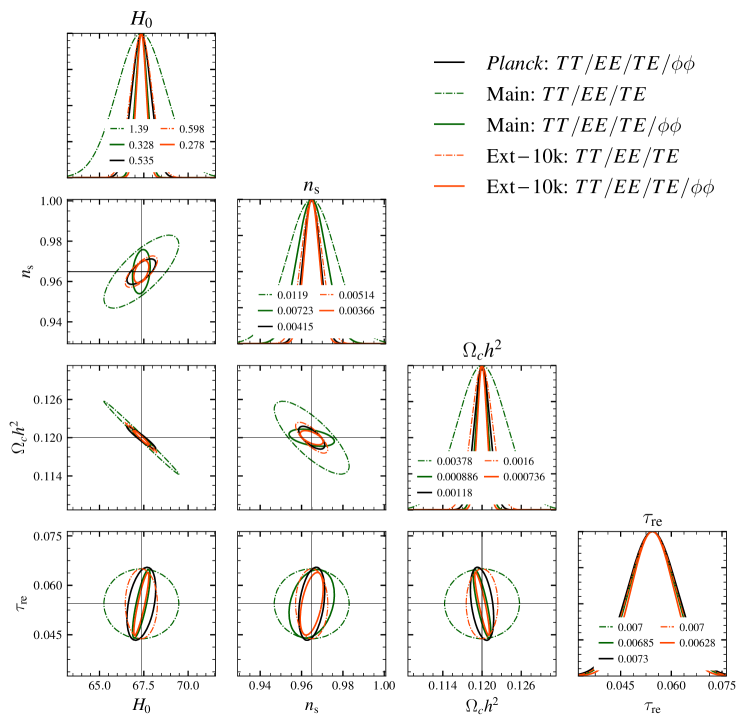
In Fig. 13, we demonstrate the parameter constraints from Planck in black, and SPT-3G Main in green and Ext-10k in orange. For SPT-3G, we show the constraints that we get from $TT/EE/TE$ CMB-only as the dash-dotted and the ones with the inclusion of lensing $\phi\phi$ as the solid curves. It is evident from the figure that the inclusion of lensing breaks parameter degeneracies, which helps in improving the constraints on many cosmological parameters.

References

Abazajian et al. (2022) Abazajian, K., Addison, G. E., Adshead, P., et al. 2022, ApJ, 926, 54, doi: 10.3847/1538-4357/ac1596
Abbott et al. (2022) Abbott, T. M. C., Aguena, M., Alarcon, A., et al. 2022, Phys. Rev. D, 105, 023520, doi: 10.1103/PhysRevD.105.023520
Ade et al. (2015) Ade, P. A. R., et al. 2015, Astron. Astrophys., 580, A22, doi: 10.1051/0004-6361/201424496
Ade et al. (2021) Ade, P. A. R., Ahmed, Z., Amiri, M., et al. 2021, Phys. Rev. Lett., 127, 151301, doi: 10.1103/PhysRevLett.127.151301
Aiola et al. (2020) Aiola, S., Calabrese, E., Maurin, L., et al. 2020, arXiv e-prints, arXiv:2007.07288. https://arxiv.org/abs/2007.07288
Alam et al. (2021) Alam, S., Aubert, M., Avila, S., et al. 2021, Phys. Rev. D, 103, 083533, doi: 10.1103/PhysRevD.103.083533
Aloni et al. (2022) Aloni, D., Berlin, A., Joseph, M., Schmaltz, M., & Weiner, N. 2022, Phys. Rev. D, 105, 123516, doi: 10.1103/PhysRevD.105.123516
Anderson et al. (2018) Anderson, A. J., Ade, P. A. R., Ahmed, Z., et al. 2018, Journal of Low Temperature Physics, doi: 10.1007/s10909-018-2007-z
Asgari et al. (2021) Asgari, M., Lin, C.-A., Joachimi, B., et al. 2021, A&A, 645, A104, doi: 10.1051/0004-6361/202039070
Balkenhol et al. (2021) Balkenhol, L., Dutcher, D., Ade, P. A. R., et al. 2021, Phys. Rev. D, 104, 083509, doi: 10.1103/PhysRevD.104.083509
Bender et al. (2018) Bender, A. N., Ade, P. A. R., Ahmed, Z., et al. 2018, in Proc. SPIE, Vol. 10708, Proc. SPIE, 1070803, doi: 10.1117/12.2312426
Benson et al. (2014) Benson, B. A., Ade, P. A. R., Ahmed, Z., et al. 2014, in Proc. SPIE, Vol. 9153, Millimeter, Submillimeter, and Far-Infrared Detectors and Instrumentation for Astronomy VII, 91531P, doi: 10.1117/12.2057305
Bianchini et al. (2020) Bianchini, F., et al. 2020, Astrophys. J., 888, 119, doi: 10.3847/1538-4357/ab6082
Bleem et al. (2015) Bleem, L. E., Stalder, B., de Haan, T., et al. 2015, ApJS, 216, 27, doi: 10.1088/0067-0049/216/2/27
Bleem et al. (2020) Bleem, L. E., Bocquet, S., Stalder, B., et al. 2020, ApJS, 247, 25, doi: 10.3847/1538-4365/ab6993
Bleem et al. (2023) Bleem, L. E., Klein, M., Abbott, T. M. C., et al. 2023, arXiv e-prints, arXiv:2311.07512, doi: 10.48550/arXiv.2311.07512
Bocquet et al. (2024) Bocquet, S., Grandis, S., Bleem, L. E., et al. 2024, SPT Clusters with DES and HST Weak Lensing. II. Cosmological Constraints from the Abundance of Massive Halos. https://arxiv.org/abs/2401.02075
Cardoso et al. (2008) Cardoso, J.-F., Le Jeune, M., Delabrouille, J., Betoule, M., & Patanchon, G. 2008, IEEE J. Sel. Top. Signal Process., 2, 735, doi: 10.1109/JSTSP.2008.2005346
Chiang & Slosar (2018) Chiang, C.-T., & Slosar, A. 2018, arXiv e-prints, arXiv:1811.03624, doi: 10.48550/arXiv.1811.03624
Chichura et al. (2022) Chichura, P. M., Foster, A., Patel, C., et al. 2022, The Astrophysical Journal, 936, 173, doi: 10.3847/1538-4357/ac89ec
Choi et al. (2020) Choi, S. K., Hasselfield, M., Ho, S.-P. P., et al. 2020, arXiv e-prints, arXiv:2007.07289. https://arxiv.org/abs/2007.07289
Copi et al. (2010) Copi, C. J., Huterer, D., Schwarz, D. J., & Starkman, G. D. 2010, Advances in Astronomy, 2010, 1–17, doi: 10.1155/2010/847541
Cyburt et al. (2016) Cyburt, R. H., Fields, B. D., Olive, K. A., & Yeh, T.-H. 2016, Reviews of Modern Physics, 88, 015004, doi: 10.1103/RevModPhys.88.015004
Cyr-Racine et al. (2022) Cyr-Racine, F.-Y., Ge, F., & Knox, L. 2022, Phys. Rev. Lett., 128, 201301, doi: 10.1103/PhysRevLett.128.201301
Dark Energy Survey and Kilo-Degree Survey Collaboration (2023) Dark Energy Survey and Kilo-Degree Survey Collaboration. 2023, The Open Journal of Astrophysics, 6, 36, doi: 10.21105/astro.2305.17173
Datta et al. (2019) Datta, R., Aiola, S., Choi, S. K., et al. 2019, MNRAS, 486, 5239, doi: 10.1093/mnras/sty2934
DES Collaboration (2024) DES Collaboration. 2024, The Dark Energy Survey: Cosmology Results With 1500 New High-redshift Type Ia Supernovae Using The Full 5-year Dataset. https://arxiv.org/abs/2401.02929
Dutcher et al. (2021) Dutcher, D., Balkenhol, L., Ade, P. A. R., et al. 2021, Phys. Rev. D, 104, 022003, doi: 10.1103/PhysRevD.104.022003
Dutcher et al. (2021) Dutcher, D., et al. 2021, Phys. Rev. D, 104, 022003, doi: 10.1103/PhysRevD.104.022003
Everett et al. (2020) Everett, W. B., Zhang, L., Crawford, T. M., et al. 2020, ApJ, 900, 55, doi: 10.3847/1538-4357/ab9df7
Finkbeiner et al. (2012) Finkbeiner, D. P., Galli, S., Lin, T., & Slatyer, T. R. 2012, Phys. Rev. D, 85, 043522, doi: 10.1103/PhysRevD.85.043522
Galli et al. (2022) Galli, S., Pogosian, L., Jedamzik, K., & Balkenhol, L. 2022, Phys. Rev. D, 105, 023513, doi: 10.1103/PhysRevD.105.023513
Galli et al. (2013) Galli, S., Slatyer, T. R., Valdes, M., & Iocco, F. 2013, Phys. Rev. D, 88, 063502, doi: 10.1103/PhysRevD.88.063502
Galli et al. (2021) Galli, S., Wu, W. L. K., Benabed, K., et al. 2021, Phys. Rev. D, 104, 023518, doi: 10.1103/PhysRevD.104.023518
Galli et al. (2014) Galli, S., Benabed, K., Bouchet, F., et al. 2014, Phys. Rev. D, 90, 063504, doi: 10.1103/PhysRevD.90.063504
Givans & Kamionkowski (2023) Givans, J. J., & Kamionkowski, M. 2023, arXiv e-prints, arXiv:2311.06196, doi: 10.48550/arXiv.2311.06196
Guns et al. (2021) Guns, S., Foster, A., Daley, C., et al. 2021, The Astrophysical Journal, 916, 98, doi: 10.3847/1538-4357/ac06a3
Gupta et al. (2019) Gupta, N., Reichardt, C. L., Ade, P. A. R., et al. 2019, MNRAS, 490, 5712, doi: 10.1093/mnras/stz2905
Hart & Chluba (2018) Hart, L., & Chluba, J. 2018, Mon. Not. Roy. Astron. Soc., 474, 1850, doi: 10.1093/mnras/stx2783
Hart & Chluba (2020a) Hart, L., & Chluba, J. 2020a, MNRAS, 493, 3255, doi: 10.1093/mnras/staa412
Hart & Chluba (2020b) —. 2020b, MNRAS, 495, 4210, doi: 10.1093/mnras/staa1426
Heymans et al. (2020) Heymans, C., Tröster, T., Asgari, M., et al. 2020, arXiv e-prints, arXiv:2007.15632. https://arxiv.org/abs/2007.15632
Hirata & Seljak (2003a) Hirata, C. M., & Seljak, U. 2003a, Phys. Rev. D, 67, 043001, doi: 10.1103/PhysRevD.67.043001
Hirata & Seljak (2003b) —. 2003b, Phys. Rev. D, 68, 083002, doi: 10.1103/PhysRevD.68.083002
Hood et al. (2023) Hood, J. C., I., Simpson, A., McDaniel, A., et al. 2023, ApJ, 945, L23, doi: 10.3847/2041-8213/acbf45
Hotinli et al. (2022) Hotinli, S. C., Meyers, J., Trendafilova, C., Green, D., & van Engelen, A. 2022, J. Cosmology Astropart. Phys, 2022, 020, doi: 10.1088/1475-7516/2022/04/020
Hou et al. (2018) Hou, Z., Aylor, K., Benson, B. A., et al. 2018, ApJ, 853, 3, doi: 10.3847/1538-4357/aaa3ef
Hu (1998) Hu, W. 1998, Astrophys. J., 506, 485, doi: 10.1086/306274
Hu & Okamoto (2002) Hu, W., & Okamoto, T. 2002, ApJ, 574, 566, doi: 10.1086/341110
Huang et al. (2020) Huang, N., Bleem, L. E., Stalder, B., et al. 2020, AJ, 159, 110, doi: 10.3847/1538-3881/ab6a96
Hughes et al. (2023) Hughes, E., Ge, F., Cyr-Racine, F.-Y., Knox, L., & Raghunathan, S. 2023, arXiv e-prints, arXiv:2311.05678, doi: 10.48550/arXiv.2311.05678
Jedamzik & Pogosian (2020) Jedamzik, K., & Pogosian, L. 2020, Phys. Rev. Lett., 125, 181302, doi: 10.1103/PhysRevLett.125.181302
Joudaki et al. (2020) Joudaki, S., Hildebrandt, H., Traykova, D., et al. 2020, A&A, 638, L1, doi: 10.1051/0004-6361/201936154
Jungman et al. (1996) Jungman, G., Kamionkowski, M., Kosowsky, A., & Spergel, D. N. 1996, Physical Review Letters, 76, 1007. http://adsabs.harvard.edu/cgi-bin/nph-bib_query?bibcode=1996PhRvL..76.1007J&db_key=AST
Khalife et al. (2023) Khalife, A., Bahrami Zanjani, M., Galli, S., et al. 2023, arXiv e-prints, arXiv:2312.09814. https://arxiv.org/abs/2312.09814
Knox (1995) Knox, L. 1995, Phys. Rev. D, 52, 4307
Knox & Millea (2020) Knox, L., & Millea, M. 2020, Phys. Rev. D, 101, 043533, doi: 10.1103/PhysRevD.101.043533
Kuijken et al. (2019) Kuijken, K., Heymans, C., Dvornik, A., et al. 2019, A&A, 625, A2, doi: 10.1051/0004-6361/201834918
Lee et al. (2023) Lee, N., Ali-Haïmoud, Y., Schöneberg, N., & Poulin, V. 2023, Phys. Rev. Lett., 130, 161003, doi: 10.1103/PhysRevLett.130.161003
Louis et al. (2014) Louis, T., Addison, G. E., Hasselfield, M., et al. 2014, J. Cosmology Astropart. Phys, 7, 016, doi: 10.1088/1475-7516/2014/07/016
Madhavacheril et al. (2020) Madhavacheril, M. S., Smith, K. M., Sherwin, B. D., & Naess, S. 2020, arXiv e-prints, arXiv:2011.02475, doi: 10.48550/arXiv.2011.02475
Madhavacheril et al. (2023) Madhavacheril, M. S., Qu, F. J., Sherwin, B. D., et al. 2023, arXiv e-prints, arXiv:2304.05203, doi: 10.48550/arXiv.2304.05203
Meiers et al. (2023) Meiers, M., Knox, L., & Schöneberg, N. 2023, Phys. Rev. D, 108, 103527, doi: 10.1103/PhysRevD.108.103527
Millea et al. (2019) Millea, M., Anderes, E., & Wandelt, B. D. 2019, Phys. Rev. D, 100, 023509, doi: 10.1103/PhysRevD.100.023509
Millea et al. (2015) Millea, M., Knox, L., & Fields, B. D. 2015, Phys. Rev. D, 92, 023010, doi: 10.1103/PhysRevD.92.023010
Millea & Seljak (2021) Millea, M., & Seljak, U. 2021, arXiv:2112.09354 [astro-ph, stat]. http://ascl.net/2112.09354
Millea et al. (2021) Millea, M., Daley, C. M., Chou, T. L., et al. 2021, ApJ, 922, 259, doi: 10.3847/1538-4357/ac02bb
Murakami et al. (2023) Murakami, Y. S., Riess, A. G., Stahl, B. E., et al. 2023, J. Cosmology Astropart. Phys, 2023, 046, doi: 10.1088/1475-7516/2023/11/046
Pan et al. (2023) Pan, Z., Bianchini, F., Wu, W. L. K., et al. 2023, arXiv e-prints, arXiv:2308.11608, doi: 10.48550/arXiv.2308.11608
Particle Data Group et al. (2020) Particle Data Group, Zyla, P. A., Barnett, R. M., et al. 2020, Progress of Theoretical and Experimental Physics, 2020, 083C01, doi: 10.1093/ptep/ptaa104
Peloton et al. (2017) Peloton, J., Schmittfull, M., Lewis, A., Carron, J., & Zahn, O. 2017, Phys. Rev. D, 95, 043508, doi: 10.1103/PhysRevD.95.043508
Planck Collaboration et al. (2014) Planck Collaboration, Ade, P. A. R., Aghanim, N., et al. 2014, A&A, 571, A12, doi: 10.1051/0004-6361/201321580
Planck Collaboration et al. (2016a) Planck Collaboration, Adam, R., Ade, P. A. R., et al. 2016a, A&A, 594, A9, doi: 10.1051/0004-6361/201525936
Planck Collaboration et al. (2016b) Planck Collaboration, Ade, P. A. R., Aghanim, N., et al. 2016b, A&A, 594, A13, doi: 10.1051/0004-6361/201525830
Planck Collaboration et al. (2020) Planck Collaboration, Aghanim, N., Akrami, Y., et al. 2020, A&A, 641, A6, doi: 10.1051/0004-6361/201833910
Qu et al. (2024) Qu, F. J., Sherwin, B. D., Madhavacheril, M. S., et al. 2024, ApJ, 962, 112, doi: 10.3847/1538-4357/acfe06
Raghunathan & Omori (2023) Raghunathan, S., & Omori, Y. 2023, ApJ, 954, 83, doi: 10.3847/1538-4357/ace0c6
Raghunathan et al. (2024) Raghunathan, S., Ade, P. A. R., Anderson, A. J., et al. 2024, arXiv e-prints, arXiv:2403.02337, doi: 10.48550/arXiv.2403.02337
Rashkovetskyi et al. (2021) Rashkovetskyi, M., Muñoz, J. B., Eisenstein, D. J., & Dvorkin, C. 2021, Phys. Rev. D, 104, 103517, doi: 10.1103/PhysRevD.104.103517
Reichardt et al. (2021) Reichardt, C. L., Patil, S., Ade, P. A. R., et al. 2021, ApJ, 908, 199, doi: 10.3847/1538-4357/abd407
Riess et al. (2022) Riess, A. G., Yuan, W., Macri, L. M., et al. 2022, ApJ, 934, L7, doi: 10.3847/2041-8213/ac5c5b
Schiappucci et al. (2023) Schiappucci, E., Bianchini, F., Aguena, M., et al. 2023, Phys. Rev. D, 107, 042004, doi: 10.1103/PhysRevD.107.042004
Schöneberg et al. (2022) Schöneberg, N., Abellán, G. F., Sánchez, A. P., et al. 2022, Phys. Rep., 984, 1, doi: 10.1016/j.physrep.2022.07.001
Schöneberg et al. (2022) Schöneberg, N., Franco Abellán, G., Pérez Sánchez, A., et al. 2022, Phys.Rept., 984, 1, doi: 10.1016/j.physrep.2022.07.001
Sekiguchi & Takahashi (2021) Sekiguchi, T., & Takahashi, T. 2021, Phys. Rev. D, 103, 083507, doi: 10.1103/PhysRevD.103.083507
Sekiguchi & Takahashi (2021) Sekiguchi, T., & Takahashi, T. 2021, Phys. Rev. D, 103, 083507, doi: 10.1103/PhysRevD.103.083507
Simard et al. (2018) Simard, G., Omori, Y., Aylor, K., et al. 2018, ApJ, 860, 137, doi: 10.3847/1538-4357/aac264
Simons Observatory Collaboration (2019) Simons Observatory Collaboration. 2019, J. Cosmology Astropart. Phys, 2019, 056, doi: 10.1088/1475-7516/2019/02/056
Slatyer & Wu (2017) Slatyer, T. R., & Wu, C.-L. 2017, Phys. Rev. D, 95, 023010, doi: 10.1103/PhysRevD.95.023010
Sobrin et al. (2018) Sobrin, J. A., Ade, P. A. R., Ahmed, Z., et al. 2018, in Proc. SPIE, Vol. 10708, Proc. SPIE, 107081H, doi: 10.1117/12.2314366
Sobrin et al. (2022) Sobrin, J. A., Anderson, A. J., Bender, A. N., et al. 2022, ApJS, 258, 42, doi: 10.3847/1538-4365/ac374f
Tandoi et al. (2024) Tandoi, C., Guns, S., Foster, A., et al. 2024, Flaring Stars in a Non-targeted mm-wave Survey with SPT-3G. https://arxiv.org/abs/2401.13525
Tegmark et al. (1997) Tegmark, M., Taylor, A. N., & Heavens, A. F. 1997, ApJ, 480, 22
Thorne et al. (2017) Thorne, B., Dunkley, J., Alonso, D., & Næss, S. 2017, MNRAS, 469, 2821, doi: 10.1093/mnras/stx949
Trendafilova (2023) Trendafilova, C. 2023, J. Cosmology Astropart. Phys, 2023, 071, doi: 10.1088/1475-7516/2023/10/071
Tristram et al. (2024) Tristram, M., Banday, A. J., Douspis, M., et al. 2024, Astronomy &; Astrophysics, 682, A37, doi: 10.1051/0004-6361/202348015
Whitehorn et al. (2016) Whitehorn, N., Natoli, T., Ade, P. A. R., et al. 2016, ApJ, 830, 143, doi: 10.3847/0004-637X/830/2/143
Zaldarriaga et al. (1997) Zaldarriaga, M., Spergel, D. N., & Seljak, U. 1997, ApJ, 488, 1, doi: 10.1086/304692

Testing the 𝚲𝚲\mathbf{\Lambda}CDM Cosmological Model with Forthcoming Measurements of the Cosmic Microwave Background with SPT-3G