Multi-Agent Clarity-Aware Dynamic Coverage with Gaussian Processes

Abstract

This paper presents two algorithms for multi-agent dynamic coverage in spatiotemporal environments, where the coverage algorithms are informed by the method of data assimilation. In particular, we show that by considering the information assimilation algorithm, here a Numerical Gaussian Process Kalman Filter, the influence of measurements taken at one position on the uncertainty of the estimate at another location can be computed. We use this relationship to propose new coverage algorithms. Furthermore, we show that the controllers naturally extend to the multi-agent context, allowing for a distributed-control central-information paradigm for multi-agent coverage. Finally, we demonstrate the algorithms through a realistic simulation of a team of UAVs collecting wind data over a region in Austria.

I Introduction

A standard mission for swarms of robots is the collection of information that varies both in time and in space over a domain of interest. To collect such information optimally in some sense, the team of robots must reason about the currently available information, the target level of confidence, the spatiotemporal evolution of the underlying information, the sensing functional, as well as coordinate the actions of the each robot.

The design of informative path planners and dynamic coverage controllers has long been of interest [1, 2, 3], with a variety of techniques proposed including Voronoi partitioning [4], sampling approaches [5, 6], grid/graph based approaches [7, 8] and ergodic search [9, 10].

However, a key limitation of these methods is that simplified heuristics are used to motivate the cost functions used in the informative path planners. For example, the ergodic-search approaches assume that a target spatial distribution is defined. However there has been less work on how one can obtain such a distribution in a principled manner.

The goal of this paper is to demonstrate how such information reward functions can be designed by explicitly considering the information assimilation algorithm used. In particular, when estimating a spatiotemporal field, a common practice is to use Gaussian processes, and treat the spatiotemporal field as a realization of a stochastic partial differential equation [11, 12]. In this case, the sensing function and process noise model are well defined, and therefore the coverage controller should respect those dynamics when designing trajectories.

This paper has three main contributions: (A) We use clarity [13] (discussed below) to quantify the rate of information collection at a position $p$ due to measurements made by a robot at a different position $x_{r}$. This quantifies the value of the robot being at a certain state $x_{r}$. (B) We use this relation to propose two coverage controllers that can be used for information gathering. (C) Being feedback controllers, we show how they can scale to the multi-agent setting. We also demonstrate the algorithms using a realistic simulation, where a team of aerial robots must explore a region of Austria, and estimate the wind speed over the domain of interest.

In our previous work, we demonstrated a connection between coverage controllers and information assimilation based on the Kalman Filter [13]. There, an information metric called clarity was introduced to quantify the quality of the information possessed about a stochastic variable. In particular, if the value of the stochastic variable was known exactly, (i.e., its differential entropy approached $-\infty$), the clarity of the random variable is 1. Similarly, if no information was possessed about this variable, the clarity is 0. In this paper, we use the properties of clarity and in particular the clarity dynamics of an environment to address contribution (A).

The paper is structured as follows. First, we present various preliminaries, and explain the problem statement addressed by this paper. Next, we discuss the information assimilation model in detail, identifying a key function that is used by the coverage controllers. Then we propose the two coverage controllers, and derive the feedback controllers. Finally, we present realistic simulations of information collection in Austria.

II Preliminaries

II-A Notation

Let $\mathbb{Z}$ be the set of integers. Let $\mathbb{R},\mathbb{R}_{\geq 0},\mathbb{R}_{>0},\overline{\mathbb{R}}=\mathbb{R}\cup\{-\infty,\infty\}$ denote the set of reals, nonnegative reals, positive reals, and extended reals respectively. Let $\mathbb{S}_{++}^{n}$ denote the set of symmetric positive definite matrices in $\mathbb{R}^{n\times n}$. Let $I$ denote the identity matrix. Let $\mathbb{H}(\mathbb{R}^{d})$ be the Hilbert Space of functions with domain $\mathbb{R}^{d}$.

II-B Clarity

The notion of “information collection” used in this paper is as follows. The goal is to estimate the value of the spatiotemporal field over a given mission domain, i.e., to decrease the uncertainty about the value of the field to a specified threshold level. To quantify this, the information metric clarity was introduced in [13], and is based on differential entropy.

Definition 1.

[14, Ch. 8] The differential entropy $h[X]\in[-\infty,\infty]$ of a continuous random variable $X$ with support $S$ and density $\rho:S\to\mathbb{R}$ is

$$h[X]=-\int_{S}\rho(x)\log\rho(x)dx.$$ (1)

Notice that when $X$ has a singleton support set, $h[X]=-\infty$. Clarity is defined in terms of differential entropy.

Definition 2.

Let $X$ be a $n$-dimensional continuous random variable with differential entropy $h[X]$. The clarity $q[X]\in[0,1]$ of $X$ is defined as:

$$q[X]=\left(1+\frac{\exp{(2h[X])}}{(2\pi e)^{n}}\right)^{-1}.$$ (2)

In other words, the clarity $q[X]$ about a random variable $X$ lies in $[0,1]$, with $q=0$ corresponding to the limiting case where the uncertainty in $X$ is infinite, and $q=1$ corresponding to the limiting case where $X$ is perfectly known in an idealized (noise-free) setting. For a scalar Gaussian random variable $X\sim\mathcal{N}(\mu,\sigma^{2})$, the clarity is $q[X]=1/(1+\sigma^{2})$.

In an estimation context, we use the clarity of our estimate to quantify the quality of our estimate: as the clarity increases towards 1, the uncertainty of our estimate decreases. In [13] it was shown that when $X$ is estimated using a Kalman filter, the clarity dynamics of the estimate of $X$ can be obtained in closed form.

II-C Gaussian Processes

A Gaussian Process (GP) [15, Ch. 2] is a (scalar) stochastic process

$$f(x)\sim GP(m(x),k(x,x^{\prime}))$$ (3)

that is fully defined by the mean and the kernel

$$m(x) =E[f(x)],$$ (4a)

$$k(x,x^{\prime}) =E[(f(x)-m(x))(f(x^{\prime})-m(x^{\prime}))],$$ (4b)

respectively, where $m:\mathcal{D}\to\mathbb{R}$, $k:\mathcal{D}\times\mathcal{D}\to\mathbb{R}$ for some domain $D\subset\mathbb{R}^{d}$. When the kernel is stationary and isotropic, i.e., it only depends on $\left\|x_{1}-x_{2}\right\|$, we overload $k$ as $k(\left\|x_{1}-x_{2}\right\|)=k(x_{1},x_{2})$. Given a set of measurements $\{(x_{k},y_{k})\}_{k=1}^{N}$, we can update our posterior estimate of $f$, as described in [15, Ch. 2].

II-D Spatiotemporal Gaussian Processes

Our goal is to estimate a spatiotemporal field, i.e., to estimate a function $f(t,p)$, $f:\mathbb{R}\times\mathcal{D}\to\mathbb{R}$. Here $t\in\mathbb{R}$ denotes time, and $\mathcal{D}\subset\mathbb{R}^{d}$ is spatial domain of interest.

We start with the prior that

$$f(t_{0},p)\sim GP(m_{0}(p),k_{0}(p,p^{\prime}))$$ (5)

for given mean and (spatial) kernel functions $m_{0}:\mathcal{D}\to\mathbb{R}$, $k_{0}:\mathcal{D}\times\mathcal{D}\to\mathbb{R}$.

As in [11], we assume the function $f$ evolves according to a linear stochastic differential process, and that (noisy) measurements $y_{k}\in\mathbb{R}$ are available at discrete times $t_{k}$:

$$df(t,p) =\mathcal{A}f(t,p)dt+dW(t,p)$$ (6a)

$$y_{k} =\mathcal{H}_{k}f(t_{k},p)+r_{k}.$$ (6b)

Here, $p\mapsto f(t,p)\in\mathbb{H}(\mathcal{D})$, and $\mathcal{A}:\mathbb{H}(\mathcal{D})\to\mathbb{H}(\mathbb{R}^{d})$ is a linear differential operator describing the evolution of $f$. $W(t,p)$ is a Wiener processes, with joint diffusion operator $Q_{c}(p,p^{\prime})$.

The measurement at time $t_{k}$ is $y_{k}\in\mathbb{R}^{r}$, i.e., the value of $f$ measured by $r$ robots, at positions $P_{r}=\{x_{i}\}_{i=1}^{r}$. Each measurement is perturbed by some $r_{k}\sim\mathcal{N}(0,R_{k})$. Therefore, the measurement operator $\mathcal{H}_{k}:\mathbb{H}(\mathbb{R}^{d})\to\mathbb{R}^{r}$ is the linear operator $\mathcal{H}_{k}f(t_{k},p)=[f(t_{k},x_{1}),\cdots,f(t_{k},x_{r})]^{T}$.

This model is a infinite-dimensional linear Ito stochastic differential equation [11]. In this work, we consider a special case to simplify the analysis. In particular, we assume $\mathcal{A}=0$, i.e., the spatiotemporal field is time-evolving only due to the Wiener process, although the methods in [11, 12] can be used to handle more general cases. Then, the corresponding discrete time model is

$$f(t_{k},p) =f(t_{k-1},p)+w_{k-1}(p)$$ (7a)

$$y_{k} =\mathcal{H}_{k}f(t_{k},p)+r_{k},$$ (7b)

where $w_{k-1}(p)\sim GP(0,Q(p,p^{\prime};\Delta t))$, $\Delta t=t_{k}-t_{k-1}$. As before, $r_{k}\sim\mathcal{N}(0,R_{k})$ for $R_{k}\in\mathbb{S}_{++}^{r}$. For simplicity, we assume $w_{k-1}(p)$ is a noise process independent at each $t$ and each $p$. Therefore $Q(p,p^{\prime};\Delta t)=\sigma_{t}^{2}(p)\delta(p-p^{\prime})\Delta t$. Although this model is in discrete time, it is still an infinite dimensional system, and not computationally tractable.

In [12], the Numerical Gaussian Process Kalman Filter (NGPKF) algorithm is developed make the above tractable. Kuper converts the infinite-dimensional model (7) into a finite-dimensional state-space model, and then employs the Kalman Filter for estimation. This reduces the computational complexity from $\mathcal{O}(N^{3})$ to $\mathcal{O}(N)$ where $N$ is the number of measurements.

As in the standard Kalman Filter (KF), let $m_{k_{2}|k_{1}}$ denote the state estimate at time $t_{k_{2}}$ using measurements upto time $t_{k_{1}}$. Let $\Sigma_{k_{2}|k_{1}}$ denote the corresponding covariance matrix.

In the NGPKF [12], the state estimate is $m_{k|k}\in\mathbb{R}^{g}$ representing the estimate of $f$ evaluated at a set of $g$ grid positions $P_{g}=\{p_{i}^{g}\}_{i=1}^{g}\subset\mathcal{D}$. The covariance is $\Sigma_{k|k}\in\mathbb{S}_{++}^{g}$. The prediction step of the NGPKF is

$$m_{k|k-1} =m_{k-1|k-1}$$ (8a)

$$\Sigma_{k|k-1} =\Sigma_{k-1|k-1}+W_{k-1},$$ (8b)

where $W_{k-1}$ is a diagonal matrix in $\mathbb{R}^{g\times g}$, with the $(i,i)$ element containing $\sigma_{t}^{2}(p_{i})$. The correction step is

$$S_{k} =C_{k}\Sigma_{k|k-1}C_{k}^{T}+V_{k}$$ (9a)

$$L_{k} =\Sigma_{k|k-1}C_{k}^{T}S_{k}^{-1}$$ (9b)

$$m_{k|k} =m_{k|k-1}+L_{k}(y_{k}-C_{k}m_{k|k-1})$$ (9c)

$$\Sigma_{k|k} =\Sigma_{k|k-1}-L_{k}S_{k}L_{k}^{T},$$ (9d)

where

$$C_{k} =K_{rg}K_{gg}^{-1}, C_{k}\in\mathbb{R}^{r\times g},$$ (10a)

$$V_{k} =K_{rr}-C_{k}K_{gr}+R_{k}, V_{k}\in\mathbb{R}^{r\times r},$$ (10b)

$$K_{rr} =K(P_{r},P_{r}), K_{rr}\in\mathbb{R}^{r\times r},$$ (10c)

$$K_{gr} =K(P_{g},P_{r}), K_{gr}\in\mathbb{R}^{g\times r},$$ (10d)

$$K_{gg} =K(P_{g},P_{g}), K_{gg}\in\mathbb{R}^{g\times g},$$ (10e)

Recall $P_{g}$ is the set of NGPKF grid positions, and $P_{r}$ are the measurement positions. The matrix $K(P_{r},P_{g})\in\mathbb{R}^{r\times g}$ denotes the kernel matrix with $k(p_{i}^{r},p_{g}^{j})$ in its $(i,j)$ entry. Note, for numerical reasons it is important to use a numerically stable version of the Kalman Filter [17].

II-E Ergodic Control

Ergodic control [9, 10] is a technique to generate trajectories of a robot to cover a domain $\mathcal{D}=[0,L_{1}]\times\cdots\times[0,L_{d}]\subset\mathbb{R}^{d}$, such that the trajectories have a spatial (position) distribution that closely matches a specified Target Spatial Distribution (TSD), as explained below.

The TSD is a function $\phi:\mathcal{D}\to\mathbb{R}$ representing a desired probability density function for where the user wants the robot to spend time. Given a trajectory $\xi:[0,T]\to\mathcal{D}$, the spatial distribution of the trajectory is defined as $c_{\xi}:\mathcal{D}\to\mathbb{R}$,

$$c_{\xi}(p)=\frac{1}{T}\int_{0}^{T}\delta(p-\xi(\tau)))d\tau$$ (11)

where $\delta:\mathbb{R}^{d}\to\mathbb{R}$ is the Dirac delta function. In words, given a trajectory $\xi$, $c_{\xi}(p)$ is the fraction of time the robot spent at a position $p\in\mathcal{D}$. Then, the ergodicity of the trajectory $\xi$ w.r.t to the TSD $\phi$, is $\mathcal{E}\in\mathbb{R}$,

$$\mathcal{E}=\left\|c_{\xi}-\phi\right\|_{H^{-s}}^{2}$$ (12)

where $\left\|\cdot\right\|_{H^{-s}}$ is the Sobolev space norm of order $s=(d+1)/2$, defined in [9]. The norm is defined by

$$\left\|c_{\xi}-\phi\right\|_{H^{-s}}^{2} =\sum_{l\in\mathbb{N}^{d}}\Lambda_{l}(\hat{c}_{l}-\hat{\phi}_{l})^{2}$$ (13)

where $\Lambda_{l}\in\mathbb{R}$ is a weighting coefficient, and $\hat{(\cdot)}_{l}$ is the $l$-th element of the discrete cosine transform of the function $\cdot$, e.g.

$$\hat{\phi}_{l}=\langle\phi_{l},b_{l}\rangle=\int_{p\in\mathcal{D}}\phi_{l}(p)b_{l}(p)dp$$ (14)

where $b_{l}:\mathcal{D}\to\mathbb{R}$ is the $l$-th basis function. We refer the reader to [9] for further details.

$\mathcal{E}$ is thus a function space norm measuring the difference between the TSD and the spatial distribution of the trajectory. The key benefit of the Sobolev norm is that it prioritizes matching the low spatial frequency differences between $c$ and $\phi$ before the high spatial frequencies. This means that the controllers have a multiscale-spectral nature, where they prioritize covering the domain globally, before returning to the gaps and covering them [9].

In [9] a feedback controller is derived for single and double integrator robot models that minimizes the ergodicity. Various extensions have been presented in, for example, [10, 18] to address other robot models and other goals.

II-F Problem Statement

In this paper, we study the design of multiagent coverage controllers that exploit the information assimilation algorithms used to model information gain. We consider a team of robots that have a control affine dynamical system,

$$\dot{x}_{r}=F(x_{r})+G(x_{r})u$$ (15)

where $x_{r}\in\mathcal{D}$ is the robot state, $u\in\mathbb{R}^{m}$ is the control input, and $F:\mathcal{D}\to\mathbb{R}^{d}$, $G:\mathcal{D}\to\mathbb{R}^{d\times m}$. Given a feedback controller $u=\pi(t,x_{r})$, $\pi:\mathbb{R}\times\mathcal{D}\to\mathcal{U}$, we assume the closed-loop system $\dot{x}_{r}=F(x_{r})+G(x_{r})\pi(t,x_{r})$ admits unique solutions.

For the sake of brevity, in this paper we use $x_{r}\in\mathcal{D}$ to denote the robot state, i.e., only considering the position of the robot. The methods can be extended to the case where the robot state also contains additional states like the velocity.

Our goal is to answer two questions: (A) how does the information assimilation algorithm inform the value of taking measurements at a robot position $x_{r}\in\mathcal{D}$ on the quality of information at a different position $p\in\mathcal{D}$, and (B) how should one design coverage controllers to exploit that relationship? Since the mission is a multiagent coverage problem, we also need to ensure that the proposed coverage algorithms should be scalable to a team of robots. We address each of these two questions in the following two sections.

III Information Assimilation

For any coverage controller, two main functions are required: (A) the information decay rate at each $p\in\mathcal{D}$ when the position $p$ is not being sensed, and (B) the information gain at each $p\in\mathcal{D}$ due to a measurement taken from the robot’s position $x\in\mathcal{D}$. In this section, we discuss how the GP model of the spatiotemporal field can be used to determine these two functions. Note, we consider the hyperparameters of the GP to be specified and constant, although some strategies for estimating these are provided in the simulation section.

In this section we focus on the single position $p\in\mathcal{D}$, and track the evolution of our estimate of $f(t,p)$. We denote our estimate $\hat{f}(t,p)=\mathcal{N}(m(t),\Sigma(t))$, where $m(t)\in\mathbb{R}$ the mean, and $\Sigma(t)\in\mathbb{R}_{>0}$ is the variance of the estimate. At discrete times $t_{k}$, we denote $m(t_{k})=m_{k}$, and similarly for $\Sigma$. As in the standard Kalman Filter, due to the measurements and process noise, $m,\Sigma$ will vary with time.

III-A Information Decay

Recall our discrete-time model,

$$f(t_{k},p) =f(t_{k-1},p)+w_{k-1}(p),$$ (16)

where $w_{k-1}(p)\sim GP(0,\sigma_{t}^{2}(p)\delta(p-p^{\prime})\Delta t)$. $\sigma_{t}:\mathcal{D}\to\mathbb{R}$ is the strength of the Wiener process. By writing $\sigma_{t}(p)$ we emphasize that the strength of the Wiener process can be different in different positions across the domain. Notice that due to the $\delta(p-p^{\prime})$, the noise added at each $p$ is independent of the noise any other $p^{\prime}$. Therefore, our prediction model takes the form

$$m_{k}=m_{k-1},\quad\Sigma_{k}=\Sigma_{k-1}+\sigma_{t}^{2}\Delta t$$ (17)

III-B Information Gain

Next, we must consider the influence of a measurement from a robot position $x_{r}\in\mathcal{D}$ on the quality of the estimate at any position $p\in\mathcal{D}$. In [13], the model

$$y_{k}=C(x_{r},p)f(t,p)+r_{k},\quad r_{k}\sim\mathcal{N}(0,R_{k})$$ (18)

was used, where

$$C(x_{r},p)=\begin{cases}1&\text{ if }\left\|x_{r}-p\right\|\leq d\\ 0&\text{ else }\end{cases}$$ (19)

representing the fact that the measurement $y_{k}$ depends on the value of the spatiotemporal field at $p$ only if the robot is sufficiently close to $p$. While this is intuitively reasonable, it is not clear how $d$ should be chosen given the properties of the spatiotemporal field.

By modeling the spatiotemporal field through a Gaussian Process, the measurement of $f$ at some position $x_{r}\in\mathcal{D}$ is correlated with the value of $f$ at another position $p\in\mathcal{D}$. We can use the spatial kernel of the GP to compute this correlation, and update our estimate of $f$ at $p$ using the measurement at $x_{r}$.

Notice that $y_{k}$ is the measurement of $f(t_{k},x_{r})$,

$$y_{k}=f(t_{k},x_{r})+r_{k},\quad r_{k}\sim\mathcal{N}(0,R_{k}),$$ (20)

but due to the correlation between $f(t_{k},p)$ and $f(t_{k},x_{r})$, $y_{k}$ can equivalently be interpreted as measurement of $f(t_{k},p)$,

$$y_{k}=C(x_{r},p)f(t_{k},p)+v_{k},\quad v_{k}\sim\mathcal{N}(0,V_{k}),$$ (21)

where using (9),

$$C(x_{r},p) =K_{rg}K_{gg}^{-1}=\frac{k(x_{r},p)}{k(p,p)}$$ (22)

$$V(x_{r},p) =K_{rr}-C(x_{r},p)K_{gr}+R_{k}$$

$$=k(x_{r},x_{r})-\frac{k(x_{r},p)k(p,x_{r})}{k(p,p)}+R_{k}.$$ (23)

Therefore, using (9), the discrete-time Kalman gain and covariance update equations can be determined.

III-C Quantifying Information Gain via Clarity Dynamics

Next, we wish to characterize the clarity dynamics, i.e., the time-evolution of the clarity about the spatiotemporal field at any position $p\in\mathcal{D}$ due to measurements taken by a robot at position $x_{r}\in\mathcal{D}$.

First, we must convert our discrete-time model into a continuous-time model. Recall $\Delta t>0$ is the sampling period. The main property we use is that for a Wiener process $W_{t}$, $W_{t_{2}}-W_{t_{1}}\sim\mathcal{N}(0,t_{2}-t_{1})$.

Using (17), the continuous-time model for $f(t,p)$ takes the form

$$\dot{f}(t,p)=w(t),\quad w(t)\sim\mathcal{N}(0,W(p))$$ (24)

where $W(p)=\sigma_{t}^{2}(p)$, and using (21), the continuous-time measurement model is

$$y=C(x_{r},p)f(t,p)+v(t),\quad v(t)\sim\mathcal{N}\left(0,\frac{V(x_{r},p)}{\Delta t}\right)$$ (25)

where we divided $V(x_{r},p)$ by $\Delta t$ to account for the measurement sampling period.

This allows us to define the clarity dynamics of the quality of our estimate of $f(t,p)$:

$$\dot{q}=\frac{C(x_{r},p)^{2}\Delta t}{V(x_{r},p)}(1-q(t,p))^{2}-W(p)q(t,p)^{2}$$ (26)

This expression was first derived in [13, Eq. 12]. To simplify the notation, let $S:\mathcal{D}\times\mathcal{D}\to\mathbb{R}$ be

$$S(x_{r},p)=\frac{C(x_{r},p)^{2}\Delta t}{V(x_{r},p)}.$$ (27)

In the case of a stationary and isotropic kernel $k(x,x^{\prime})=k(\left\|x-x^{\prime}\right\|)$, the expression simplifies to

$$S(x_{r},p) =\frac{k(\left\|x_{r}-p\right\|)^{2}\Delta t}{k(0)^{2}(1+R_{k})-k(\left\|x_{r}-p\right\|)^{2}}$$ (28)

If $d\mapsto k(d)$ is monotonically decreasing, e.g. in the Matern and Squared Exponential kernels, $S(x_{r},p)$ is maximized at $x_{r}=p$, implying that the rate of increase in clarity about $p$ is maximized when the robot is at $x_{r}=p$. This is not in general true, since for example in periodic or polynominal kernels, $S(x_{r},p)$ may be maximized for some $x_{r}\neq p$.

To summarize, we are solving an information gathering problem where the spatiotemporal information to be collected is modeled using a Gaussian Process. To define a suitable coverage algorithm, we require a method to quantify the value of taking a measurement at some robot position $x_{r}\in\mathcal{D}$ on the information gain at all points $p\in\mathcal{D}$. This is captured by the clarity dynamics, i.e., the relationship that quantifies the rate of information gain as:

$$\dot{q}=S(x_{r},p)(1-q(t,p))^{2}-W(p)q(t,p)^{2},$$ (29)

The key function is $S$, as defined in (27). Notice that only the first term $S(x_{r},p)$ is controllable, since it is the only term that depends on the robot’s position $x_{r}$.

IV Coverage Controllers

In this section, we derive two coverage controllers that use (29). The direct method aims to choose a control input that maximizes the rate of increase in the total clarity integrated over the domain $\mathcal{D}$. The indirect method determines the time that the robot should spend at each position in the domain to achieve a target clarity, and then uses Ergodic control to compute the control input.

IV-A Direct Method

Consider a cost function of the form

$$J(t)=\left\|\overline{q}(\cdot)-q(t,\cdot)\right\|_{\ell_{2}}^{2}=\int_{p\in\mathcal{D}}(\overline{q}(p)-q(t,p))^{2}dp$$ (30)

i.e., the $\ell_{2}$-norm of the difference between the current clarity $q(t,p)$ and the target clarity $\overline{q}(p)$. Then, to determine the best control input, the objective is to minimize $J$ over a short horizon $\delta t$ in the future:

$$J(t+\delta t)=J(t)+\dot{J}(t,x)\delta t^{2}+\frac{1}{2}\ddot{J}(t,x,u)\delta t^{2}$$ (31)

where the dependency on $u$ first shows up in the $\ddot{J}$ term. This high-relative degree behaviour is a consequence of the fact that the clarity dynamics (29) depend on $x$, not $\dot{x}$. Therefore the second derivative of $J$ must be taken for the control input to appear in the expressions. This behaviour is commonly observed in the literature on coverage control, as in [3, Ch. 2] and in [9].

In [3], a control input to minimize $\ddot{J}(t,x,u)$ is derived, and used as the coverage controller. A differentiable sensing functional (an analog of $S(x_{r},p)$ defined above) is used with the generalized transport theorem to compute $\ddot{J}(t,x,u)$. However this approach often leads to local minima, where $\ddot{J}(t,x,u)$ becomes independent of $u$. This happens when all of the local information has been collected, and there is no preference for the controller to move in one direction over the other. To address this, [3] proposed combining the local search strategy with a global strategy, where the controller would choose a new global waypoint when the local control strategy reached a local minima.

We propose an extension of the controller in [3] to address two of its limitations. In particular, we propose using the sensing function $S(x,p)$ derived in the previous section to compute $J,\dot{J},\ddot{J}$. Second, we replace $\ell_{2}$ norm in the cost function with the $H$-norm proposed by [9]. This causes the control input to be selected to maximize global clarity levels before local clarity levels, i.e., the lower spatial frequencies of the clarity are minimized before the higher spatial frequencies.

Consider the cost function

$$J(t) =\left\|\overline{q}(\cdot)-q(t,\cdot)\right\|_{H^{-(d+1)/2}}^{2}=\sum_{l\in\mathbb{N}^{d}}\Lambda_{l}\left(\hat{\overline{q}}_{l}-\hat{q}_{l}(t)\right)^{2}$$ (32)

where $\hat{\overline{q}}_{l}=\langle\overline{q},b_{l}\rangle$, $\hat{q}_{l}(t)=\langle q_{l}(t,\cdot),b_{l}\rangle$. Recall the notation $\langle a,b_{l}\rangle$, $\Lambda_{l}$ was defined in Section II-E. After some algebraic calculations, one can show that the first and second time derivatives of $J$ are written as:

$$\dot{J}(t,x) =\sum_{l\in\mathbb{N}^{d}}-2\Lambda_{l}(\hat{\overline{q}}_{l}-\hat{q}_{l}(t))\dot{\hat{q}}_{l}(t,x)$$ (33)

$$\ddot{J}(t,x,u) =\sum_{l\in\mathbb{N}^{d}}2\Lambda_{l}\left(\dot{\hat{q}}_{l}^{2}(t,x)-(\hat{\overline{q}}_{l}-\hat{q}_{l}(t))\ddot{\hat{q}}_{l}(t,x,u)\right)$$ (34)

where $\dot{\hat{q}}_{l}(t,x),\ddot{\hat{q}}_{l}(t,x,u)$ are as follows:

$$\dot{\hat{q}}_{l} =\frac{d}{dt}\int_{p\in\mathcal{D}}q(t,p)b_{l}(p)dp$$ (35)

$$=\int_{p\in\mathcal{D}}\left(S(x,p)(1-q(t,p))^{2}-W(p)q(t,p)^{2}\right)b_{l}(p)dp$$ (36)

where $S$ is as defined in (27). Similarly,

$$\ddot{\hat{q}}_{l} =\frac{d^{2}}{dt^{2}}\int_{p\in\mathcal{D}}q(t,p)b_{l}(p)dp$$ (37)

$$=\hat{B}_{l}(t,x)\dot{x}+O.T.$$ (38)

where $\dot{x}=F(x)+G(x)u$ and $\hat{B}_{l}(t,x)\in\mathbb{R}^{1\times d}$ is as defined as

$$\hat{B}_{l}(t,x) =\int_{p\in\mathcal{D}}(1-q(t,p))^{2}\frac{\partial S}{\partial x}(x,p)b_{l}(p)dp$$ (39)

$$=\left\langle(1-q(t,\cdot))^{2}\frac{\partial S}{\partial x}(x,\cdot),b_{l}\right\rangle$$ (40)

and $O.T.$ collects all other terms that do not depend on $\dot{x}$ (and therefore $u$). Therefore, we have

$$J(t+\delta) =\frac{1}{2}\ddot{J}(t)\delta^{2}+O.T.$$ (41)

$$=\delta^{2}\sum_{l\in\mathbb{N}^{d}}-\Lambda_{l}(\hat{\overline{q}}_{l}-\hat{q}_{l}(t))\hat{B}_{l}(t,x)\dot{x}+O.T.$$ (42)

$$=-\delta^{2}L(t,x)(F(x)+G(x)u)+O.T.$$ (43)

where

$$L(t,x)=\sum_{l\in\mathbb{N}^{d}}\Lambda_{l}(\hat{\overline{q}}_{l}-\hat{q}_{l}(t))\hat{B}_{l}(t,x).$$ (44)

Therefore, the choice of $u$ that minimizes $J(t+\delta)$ yields a feedback controller $\pi_{dir}:\mathbb{R}\times\mathcal{D}\to\mathcal{U}$,

$$\pi_{dir}(t,x)=\underset{u\in\mathcal{U}}{\text{argmin}}\ -L(t,x)G(x)u$$ (45)

Thus, if $\mathcal{U}=\{u\in\mathbb{R}^{m}:\left\|u\right\|\leq u_{max}\}$, and $L(t,x)G(x)\neq 0$,

$$\pi_{dir}(t,x)=u_{max}\frac{G(x)^{T}L^{T}(t,x)}{\left\|L(t,x)G(x)\right\|}.$$ (46)

Proving that $L(t,x)G(x)\neq 0$ for any $t,x$ is non-trivial, and will be studied in future work.

IV-B Indirect Method

The second approach is inspired by ergodic control. Ergodic control uses a Target Spatial Distribution (TSD) to determine the feedback control law, as discussed in Section II-E. Here we derive a principled method to construct the TSD based on the information assimilation algorithm discussed in Section III.

The key idea is to set the TSD to be the time required for the clarity of our estimate of $f$ to increase from its current value to a specified target clarity $\overline{q}(p)$, assuming the robot was making measurements from $x=p$.

To compute this, recall the clarity dynamics in (29). As noted in [13], the equation admits a closed-form solution. Using the notation of this paper, the clarity of our estimate of $f(t,p)$ increases from an initial value of $q_{0}$ according to

$$q(t)=q_{\infty}\left(1+\frac{2\gamma_{1}}{\gamma_{2}+\gamma_{3}\exp{(2\gamma_{0}Qt)}}\right)$$ (47)

where $\gamma_{0}=\sqrt{S(x,p)/W(p)}$, $q_{\infty}=\gamma_{0}/(1+\gamma_{0})$, $\gamma_{1}=q_{\infty}-q_{0}$, $\gamma_{2}=\gamma_{1}(\gamma_{0}-1)$, $\gamma_{3}=(\gamma_{0}-1)q_{0}-\gamma_{0}$.

Assuming $q_{0}\leq q_{f}<q_{\infty}$, the expression can be inverted to yield

$$\tau(q_{0},q_{f})=\frac{1}{2\gamma_{0}Q}\log\left(\frac{2\gamma_{1}q_{\infty}+\gamma_{2}(q_{\infty}-q_{f})}{\gamma_{3}(q_{f}-q_{\infty})}\right)$$ (48)

which is a closed-form expression for the amount of time a robot needs to spend at position $x$ such that the clarity of $p$ increases from $q_{0}$ to $q_{f}$.

Therefore, given the target clarity distribution $\overline{q}(p)$, and the current clarity distribution $q(t,p)$, the TSD at time $t$ can be specified as follows:

$$TSD(t,p)=\begin{cases}\tau(q(t,p),\overline{q}(p))&\text{ if }q(t,p)<\overline{q}(p)\\ 0&\text{ else }\end{cases}$$ (49)

Finally, we can use the ergodic control method described in [9] to design a feedback controller for the system,

$$\pi_{ind}(t,x)=\pi_{ergo}(t,x,TSD)$$ (50)

This method is similar to the coverage controller in [19], except that the TSD is computed based on the NGPKF information assimilation algorithm. More specifically, [19] utilizes a heuristic method to construct the $C(x,p)$, $R(x,p)$ and $Q(p)$ functions, where as in this paper we construct and demonstrate principled methods to obtain these functions.

IV-C Extension to Multi-Robot Coverage Control

Our proposed coverage controllers have been presented for the single-robot cases above. Here we discuss the extension and implementation of these methods in the multi-agent case, where multiple robots have to decide how to move to collect information. We assume that they are able to synchronize their information by sharing $q(t,p)$ over a centralized setting, i.e., that they are connected over a complete graph so that each robot has access to the clarity maps of its neighbors. The extensions to distributed settings are left for future work.

Notice that both proposed controllers are feedback controllers, depending on the robot’s position, and the map of the clarity over $\mathcal{D}$. Therefore, assuming each agent shares access to the clarity map, the control input for each agent $i$ can be computed simply as

$$u_{i}=\pi(t,x_{i})$$ (51)

where $x_{i}$ denotes the position of the $i$-th agent, and $\pi\in\{\pi_{dir},\pi_{ind}\}$ can be either control strategy. In the indirect approach, we must also share the history of positions visited by the agents. Here, we can also impose other constraints, for example safety constraints using CBFs, or energy constraints using the strategy in [19].

As the robots move using the coverage controllers, the robots make measurements of the spatiotemporal field from their respective positions. These measurements are assimilated into a single estimate of the spatiotemporal field using the NGPKF algorithm. The information assimilation is currently performed centrally, although future work will look into distributed methods of maintaining the estimate.

Furthermore, note that the amount of data communicated is minimal. Consider a central robot performing the NGPKF algorithm. Each robot streams measurements to the central robot, effectively sending a tuple $(t,x_{i},y_{i})$ that only consists of $d+2$ floats for each measurement. The central robot performs the data assimilation, and creates an updated clarity map. Notice that in both the direct and the indirect approaches, only the Discrete Cosine Transform (DCT) of the clarity map is needed to compute the control inputs. Therefore, the central robot can perform the DCT, and only send a small number of the most significant components of the DCT back to each robot.

V SIMULATIONS

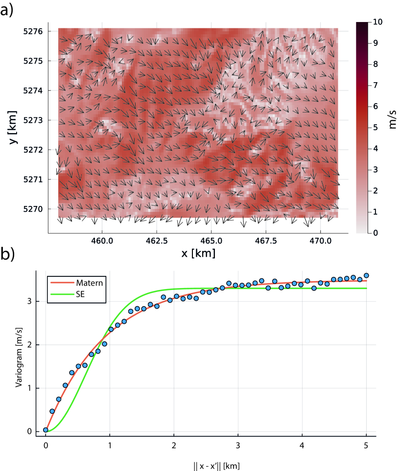
Figure 1: Wind data from WegenerNet [20]. (a) Wind speed and direction on Jan 1 2023, 00:00, (b) Variogram showing the spatial correlation within the data, with the fit from two kernels, the Matern-1/2 kernel and the squared exponential kernel.

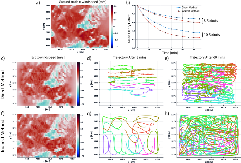
Figure 2: Simulation results. (a) shows the ground truth wind speed at the end of the simulation wind. (b) shows the mean clarity deficit over the simulation horizon. (c-e) show the behaviour of the direct method. (f-h) show the behaviour of the indirect method. (c, f) show the reconstructed wind speed. Only the x-component is visualized in the interest of space. (d, e, g, h) show the trajectories of the 10 robots after 8 minutes and after 60 minutes.

In this section, we report simulation results of an information gathering mission. As a prototypical example, we consider the collection of wind data using a team of 10 aerial robots. The robots perform a 1 hour mission, and we aim to maximize the clarity of the wind field over the domain by the end of the mission. Our evaluation metric is both the accuracy of the reconstruction, as well as the average clarity deficit, i.e., the average of $\max{(0,\overline{q}(p)-q(t,p))}$ over the mission domain.

The mission domain is a $12.7\times 6.3$ km² region of southeastern Austria, located near 46.93^∘ N, 15.90^∘ E, chosen because of a high quality ground-truth data set available through WegenerNet [20]. The dataset provides wind speeds over the domain at a resolution of 100 m and 30 minutes. The mission domain is particularly challenging due to its high weather and climate variability [20]. Over the domain considered, the maximum wind speed is less than 13 m/s.

Each robot is capable of measuring the local wind speed and direction, at a sampling period of 5 seconds. Each measurement is perturbed by noise with $\sigma_{meas}=\sqrt{R_{k}}=0.5$ m/s. The robots are assumed to have a top speed of 30 m/s, modeled as single integrators. To construct the wind field estimate from all the measurements, we use the NGPKF algorithm, using a grid with spatial resolution of $200$ m.

The spatial and temporal hyperparameters were estimated using techniques from geostatistics [21, 22]. In particular, we constructed a variogram of the dataset and used a least-squares fit to both the Matern-1/2 and the Squared Exponential kernels. The results of the fit are depicted in Figure 1b, where the Matern kernel fits the data better. The resulting kernel is of the form $k(x,x^{\prime})=\sigma^{2}\exp{\left(-\left\|x-x^{\prime}\right\|/L\right)}$, where $\sigma=3.49$ m/s, $L=0.944$ km. Fitting the kernel using the variogram was computationally much faster and more accurate than the nonlinear minimization of the log-likelihood method of [15], and the details of the procedure are listed in the appendix. The temporal length scale was estimated independently at each grid position, by computing $\sigma_{t}^{2}(p)=\text{var}\left[\frac{f(t_{2},p)-f(t_{1},p)}{t_{2}-t_{1}}\right]$ from the WegenerNet data.

Simulations were run using both the direct and the indirect control strategies, and the results are summarized in Figure 2. Both methods explore the environment, and collect information. From Fig b. we can see that the indirect method seems to decrease the mean clarity deficit faster than the direct method in these simulations.

Comparing Fig. 2a, c, f one can see that the wind speed is estimated well by both methods, although the direct method captures less information near the edges of the domain. This results in a poorer estimate near the boundaries when using the direct method.

The trajectories of the two methods are remarkably different - in the direct method, the trajectories are jagged, and the controller tends to rapidly move around as it prioritizes collecting local information first. This is because of the $\frac{\partial S}{\partial x}$ term in (40), which emphasizes the collection of data locally. In contrast, the indirect method creates smooth trajectories that cover the domain.

In Fig. 2b, we also compare the behaviour when using 3 robots against the behaviour when using 10 robots. We plot the mean clarity deficit against time for both algorithms with 3 and 10 robots, and we can see that, as expected, when there are 10 agents, the mean clarity deficit is lower than when there are only 3 agents. Fig 2 c-h show the behaviour with 10 agents.

VI CONCLUSIONS

In conclusion, this paper addresses the design of cooperative multiagent coverage controllers, where the information is shared centrally, but the control decisions are made by each robot independently. We identified a gap between information assimilation algorithms and coverage controllers. Therefore we proposed a method to quantify the value/impact that taking measurements in a domain has on the clarity of our estimate of other parts of the domain. To this end we utilized Gaussian Processes to model the environment, as well as our earlier work on the clarity dynamics, which in effect quantifies the information gain about the domain due to measurements. We saw that the relative value of measurements is captured by a function $S$. We used this function to propose two new coverage controllers that, although qualitatively different, still cover the domain and collect information accurately. The concepts were demonstrated through a simulation study of collecting information about a wind field.

A key limitation of this work is that we assumed the spatial and temporal hyperpararameters of the Gaussian Process were fixed and known apriori. Although a method was described to obtain these hyperparameters from data, in our future work we will aim to develop an online method to estimate the hyperparameters, and chose trajectories that improve the quality of the hyperparameters. Furthermore, we believe further attention should be placed on the numerical implementation of the proposed direct method, to investigate methods to obtain smooth trajectories. Finally, it would also be interesting to look into methods to ensure safety of the robots with a safety constraint that depends on the information collected online. In such a scenario, the objective of collecting information must be weighed against the importance of not violating safety constraints.

References

- [1] J. Liang, M. Liu, and X. Kui, “A survey of coverage problems in wireless sensor networks,” Sensors & Transducers, vol. 163, no. 1, p. 240, 2014.
- [2] S. Oktug, A. Khalilov, and H. Tezcan, “3d coverage analysis under heterogeneous deployment strategies in wireless sensor networks,” in 2008 Fourth Advanced International Conference on Telecommunications. IEEE, 2008, pp. 199–204.
- [3] W. Bentz, “Dynamic coverage control and estimation in collaborative networks of human-aerial/space co-robots,” Ph.D. dissertation, University of Michigan, Ann Arbor, 2020.
- [4] J. Cortes, S. Martinez, T. Karatas, and F. Bullo, “Coverage control for mobile sensing networks,” IEEE Transactions on robotics and Automation, vol. 20, no. 2, pp. 243–255, 2004.
- [5] B. Moon, S. Chatterjee, and S. Scherer, “Tigris: An informed sampling-based algorithm for informative path planning,” in 2022 IEEE/RSJ International Conference on Intelligent Robots and Systems (IROS). IEEE, 2022, pp. 5760–5766.
- [6] A. Bry and N. Roy, “Rapidly-exploring random belief trees for motion planning under uncertainty,” in 2011 IEEE international conference on robotics and automation. IEEE, 2011, pp. 723–730.
- [7] N. Cao, K. H. Low, and J. M. Dolan, “Multi-robot informative path planning for active sensing of environmental phenomena: A tale of two algorithms,” arXiv preprint arXiv:1302.0723, 2013.
- [8] C. Xiao and J. Wachs, “Nonmyopic informative path planning based on global kriging variance minimization,” IEEE Robotics and Automation Letters, vol. 7, no. 2, pp. 1768–1775, 2022.
- [9] G. Mathew and I. Mezić, “Metrics for ergodicity and design of ergodic dynamics for multi-agent systems,” Physica D: Nonlinear Phenomena, vol. 240, no. 4-5, pp. 432–442, 2011.
- [10] L. Dressel and M. J. Kochenderfer, “Tutorial on the generation of ergodic trajectories with projection-based gradient descent,” IET Cyber-Physical Systems: Theory & Applications, vol. 4, no. 2, pp. 89–100, 2019.
- [11] S. Sarkka and J. Hartikainen, “Infinite-dimensional kalman filtering approach to spatio-temporal gaussian process regression,” in Artificial intelligence and statistics. PMLR, 2012, pp. 993–1001.
- [12] A. Küper and S. Waldherr, “Numerical gaussian process kalman filtering for spatiotemporal systems,” IEEE Transactions on Automatic Control, vol. 68, no. 5, pp. 3131–3138, 2022.
- [13] D. R. Agrawal and D. Panagou, “Sensor-based planning and control for robotic systems: Introducing clarity and perceivability,” IEEE Control Systems Letters, 2023.
- [14] T. M. Cover, Elements of information theory. John Wiley & Sons, 2006.
- [15] C. K. Williams and C. E. Rasmussen, Gaussian processes for machine learning. MIT press Cambridge, MA, 2006, vol. 2, no. 3.
- [16] Z. Chen, J. Fan, and K. Wang, “Multivariate gaussian processes: definitions, examples and applications,” Metron, vol. 81, no. 2, pp. 181–191, 2023.
- [17] K. Tracy, “A square-root kalman filter using only qr decompositions,” arXiv preprint arXiv:2208.06452, 2022.
- [18] D. Dong, H. Berger, and I. Abraham, “Time optimal ergodic search,” arXiv preprint arXiv:2305.11643, 2023.
- [19] K. B. Naveed, D. Agrawal, C. Vermillion, and D. Panagou, “Eclares: Energy-aware clarity-driven ergodic search.” IEEE, 2024.
- [20] C. Schlager, G. Kirchengast, and J. Fuchsberger, “Generation of high-resolution wind fields from the wegenernet dense meteorological station network in southeastern austria,” Weather and Forecasting, vol. 32, no. 4, pp. 1301–1319, 2017.
- [21] H. Wackernagel, Multivariate geostatistics: an introduction with applications. Springer Science & Business Media, 2003.
- [22] R. B. Christianson, R. M. Pollyea, and R. B. Gramacy, “Traditional kriging versus modern gaussian processes for large-scale mining data,” Statistical Analysis and Data Mining: The ASA Data Science Journal, vol. 16, no. 5, pp. 488–506, 2023.