Double polytropic cosmic acceleration from the Murnaghan equation of state

Abstract

We consider a double polytropic cosmological fluid and demonstrate that, when one constituent resembles a bare cosmological constant while the other emulates a generalized Chaplygin gas, a good description of the Universe’s large-scale dynamics is obtained. In particular, our double polytropic reduces to the Murnaghan equation of state, whose applications are already well established in solid state physics and classical thermodynamics. Intriguingly, our model approximates the conventional $\Lambda$CDM paradigm while reproducing the collective effects of logotropic and generalized Chaplygin fluids across different regimes. To check the goodness of our fluid description, we analyze first order density perturbations, refining our model through various orders of approximation, utilizing $\sigma_{8}$ data alongside other cosmological data sets. Encouraging results suggest that our model, based on the Murnaghan equation of state, outperforms the standard cosmological background within specific approximate regimes and, on the whole, surpasses the standard phenomenological reconstruction of dark energy.

I Introduction

The current cosmic speed-up, supported by several observations Perlmutter et al. (1998); Riess et al. (1998); Perlmutter et al. (1999); Tonry et al. (2003); Bridle et al. (2003); Bennett et al. (2003); Hinshaw et al. (2003); Kogut et al. (2003); Spergel et al. (2003); Eisenstein et al. (2005), is widely attributed to an unknown exotic fluid with a negative equation of state (EoS) Sahni and Starobinsky (2000); Copeland et al. (2006); Tsujikawa (2011); Copeland et al. (2006); Maia et al. (2009); Bamba et al. (2012), well described by the cosmological constant $\Lambda$ purported by the concordance model Padmanabhan (2003) or, more broadly, by some sort of dark energy contribution Peebles and Ratra (2003), behaving anti-gravitationally Luongo and Quevedo (2014); Giambò et al. (2020); Luongo et al. (2024); Luongo and Quevedo (2023). The dark energy nature is still poorly understood Capozziello et al. (2013), but several models have been proposed either to explain the cosmic acceleration Linder and Scherrer (2009); Perković and Štefančić (2020); Bagla et al. (2003); Schmidt (2007); Nojiri et al. (2017); Luongo and Quevedo (2018); Bamba et al. (2013), or to solve the conceptual and theoretical issues raised by observed cosmological tensions Weinberg (1989); Luongo and Muccino (2018); Gruber and Luongo (2014).

Dark matter is a completely different component that represents a further challenge for modern cosmology del Campo et al. (2012), specifically the identification of its particle candidates Arbey and Mahmoudi (2021), among which we include ultralight fields, extremely massive particles, geometric contributions, or proposed extensions of Einstein’s gravity Arbey and Mahmoudi (2021); Profumo et al. (2019); Capozziello et al. (2018), without conclusive evidences in favour of any of them Pérez de los Heros (2020).

Recently, a number of unified theories Avelino et al. (2008) have been proposed to unify both dark energy and dark matter into a single dark fluid Beça and Avelino (2007) with a negative net pressure able to drive the cosmic acceleration Bento and Bertolami (1999) and treat the dark sector in the same way at the perturbative level for structure formation Hu and Eisenstein (1999). However, unified dark energy models like dark fluids Aviles and Cervantes-Cota (2011) and logotropic models Chavanis (2015) are still incomplete and have been severely criticised Fabris et al. (2011); Luongo and Quevedo (2014); Luongo and Muccino (2018); Boshkayev et al. (2021).

In order to overcome the above issues and construct a unified dark energy model, a double field approach in which a tachyonic field is minimally-coupled to a further scalar, carrying vacuum energy, has been proposed in Ref. Dunsby et al. (2024). This scenario leads to a single effective fluid that behaves pressure-less at early times, while providing a negative pressure at late times. The advantage of this recipe is that the tachyonic field behaves similarly to previous unified dark energy models, like the Chaplygin gas model Bento et al. (2002), but also includes quantum fluctuations due to a symmetry breaking mechanism associated with the field transporting vacuum energy Dunsby et al. (2024).

In this paper, we notice that a possible macroscopic interpretation of the above unified scalar fields has been phenomenologically obtained within the context of solid state physics through the introduction of the Murnaghan EoS Murnaghan (1944a). It follows that our effective cosmological matter is no longer a dust-like fluid, thus affecting the clustering of structures in a different way than the $\Lambda$CDM model during early times. Hence, physical consequences of the fact that the Murnaghan EoS yields the concept of matter with pressure are thus investigated. To do so, we propose a double polytropic interpretation of the Murnaghan EoS and show that it can reduce to the $\Lambda$CDM, logotropic and generalized Chaplygin gas (GCG) models at different epochs of the Universe evolution. Particularly, we first constrain the model free parameters and assess its compatibility with observations. Accordingly, we work with Markov chain Monte Carlo (MCMC) simulations, based on the Metropolis-Hastings algorithm and employ the most recent low-redshift $z$ catalogs such as the observational Hubble data (OHD) (Moresco et al., 2022), type Ia supernovae (SNe Ia) Scolnic et al. (2018), the observed growth function and the RMS mass fluctuations Paul and Thakur (2013). Afterwards, we compare our findings with the standard $\Lambda$CDM model. Then, using our outcomes, we study the thermodynamic behaviour of the Murnaghan fluid to compare and contrast it with other unified dark energy models. Since the Murnaghan EoS exhibits a “chameleon” behavior at different scales, we show its adaptability and propose the concept of matter with pressure as a robust candidate to describe the large-scale dynamics.

The paper is structured as follows. In Section II we introduce the Murnaghan EoS and its limiting cases. Section III deals with the numerical analysis and Section IV with the physical interpretation of the results. Section V shows the impact of matter with pressure in linear perturbations. Finally in Section VI we conclude this work and summarize our conclusions.

II The Murnaghan equation of state

In studies of stellar structure, polytropic EOSs are widely used because they suggest specific forms of heat capacities for astrophysical compact objects. In recent years, polytropic fluids have also been applied within the context of cosmological modeling with promising results Muccino et al. (2021). Specifically, the impact on structure formation can be investigated by assuming a single-fluid polytropic EoS of the form,

$$P=P_{0}\rho^{1+\gamma}\,,$$ (1)

where $\gamma=1/n$, $n\in\mathbb{N}$, the polytropic index, and, by virtue of the adiabatic sound speed defined as,

$$c_{s}^{2}\equiv\frac{\partial P}{\partial\rho},$$ (2)

one immediately obtains through Eq. (1),

$$c_{s}^{2}=P_{0}(1+\gamma)\rho^{\gamma}\neq 0\,.$$ (3)

This clearly cannot be zero since $\gamma\neq-1$ and, so, this fact clearly fixes a non-zero Jeans length, reducing the regions to form structure.

However, a genuine cosmological constant, defined as $\gamma\rightarrow-1$, would imply $c_{s}=0$, leading to an always zero Jeans length. We also notice that when $\gamma=-2$ the EoS resembles the Chaplygin gas model $P=P_{0}/\rho$, further reinforcing the idea that relaxing the hypothesis $\gamma=1/n$ would open new avenues in the physics of polytropes.

Motivated by the above considerations, a different perspective can arise if one considers a double polytropic fluid where one can introduce an additional parameter to account for the behavior of dark energy at different energy densities. This is identified by the following relation Dunsby et al. (2016),

$$P=P_{1}\rho^{1+\gamma_{1}}+P_{2}\rho^{1+\gamma_{2}}\,,$$ (4)

with $P_{1},P_{2},\gamma_{1},\gamma_{2}$ denoting unbounded constants related to different behaviours of the fluid at different energy density regimes, whose signs are unfixed. Adopting Eq. (2), we now obtain,

$$c_{s}^{2}=P_{1}(1+\gamma_{1})\rho^{\gamma_{1}}+P_{2}(1+\gamma_{2})\rho^{\gamma_{2}},$$ (5)

and notice that there exists a region where, for certain values of the free parameters, the squared of the sound speed equals zero, in analogy to dust.

This model falls into the set of unified dark energy models, made up by one single fluid only that behaves differently throughout the Universe evolution, mimicking both dark matter and dark energy at the same time. Through this interpretation, we find that the corresponding EoS is zero for stages of the Universe’s evolution and deviates in this manner from the standard dust-like assumption for matter.

We can easily construct the simplest case found in solid state physics, known as the Murnaghan fluid, by setting $\gamma_{1}<0$, but $\neq-1$, and $\gamma_{2}=0$, while identifying $P_{2}$ with the constant value of some sort of vacuum energy, to have Dunsby et al. (2024),

$$P=\frac{P_{1}}{\rho^{\beta}}+P_{2}\,,$$ (6)

where $\beta\equiv|\gamma_{1}|$. In other words, assuming Eq. (6) implies the existence of a matter-like fluid that for very large densities behaves as a constant. We find that the double polytropic EoS is analogous to the EoS given for a Murnaghan fluid, which describes the incompressibility of matter under high pressure Murnaghan (1944b).

Hence, we assume that matter in the universe provides a bulk modulus of incompressibility at constant temperature $T$, given by $K=-V(\partial P/\partial V)_{T}=K_{0}+K_{0}^{\prime}P$, with $K^{\prime}\equiv\partial K/\partial P$, that establishes a relationship between the volume $V$ and the pressure $P$ of the universe through

$$P=\frac{K_{0}}{K_{0}^{\prime}}\left[\left(\frac{V}{V_{0}}\right)^{-K_{0}^{\prime}}-1\right]\,,$$ (7)

where the subscript “$0$” denotes when $P=0$. To well adapt this recipe to the dynamics of the Universe, we additionally require that

• $P=0$ occurs when pressure-less matter dominates, namely, at a density $\rho_{\star}$ or at volume $V_{0}\propto\rho_{\star}^{-1}$;

• as $P\neq 0$, the volume $V\propto\rho^{-1}$ is larger than $V_{0}$, or $\rho_{\star}>\rho$, to ensure late time expansion;

• $K>0$, thus $K_{0}>0$, when $P=0$, and $K_{0}^{\prime}<0$, when $P<0$ to ensure the accelerated expansion of the Universe.

We can change the variables from the original EoS such that $K_{0}\rightarrow A_{\star}$ and $K_{0}^{\prime}\rightarrow-\alpha$, with $\alpha$ and $A_{\star}$ being positive constants, to obtain a GCG, $P\propto\rho^{-\alpha}$, with an extra constant Bento et al. (2002), resulting in the recast version of Eq. (6) given by,

$$P=-\frac{A_{\star}}{\alpha}\left[\left(\frac{\rho_{\star}}{\rho}\right)^{\alpha}-1\right]\,.$$ (8)

The dark fluid density in terms of the scale factor, $a=(1+z)^{-1}$, can be obtained by solving the continuity equation

$$\frac{d\rho}{da}+\frac{3}{a}(P+\rho)=0\,.$$ (9)

However, since the solution is not analytical, thus, to constrain $A_{\star}$, $\alpha$, and $\rho_{\star}$, we then explore below some approximate regimes, directly coming from Eq. (8).

• The $\Lambda$CDM approximation:
  At redshift $z\approx 0$, or $a=a_{0}\approx 1$, $\rho$ approaches the critical value $\rho_{c}=3H_{0}^{2}/(8\pi G)$, where $H_{0}$ is the Hubble constant and $G$ is the gravitational constant. Thus, for $\alpha\gtrsim 0$, we obtain,

  $$\rho(a) \approx\rho_{c}\left(\Omega_{\rm DF}+\frac{P}{\rho_{c}}\right)a^{-3}-P\,,$$ (10a)

  $$P \approx-A_{\star}\ln\left(\frac{\rho_{\star}}{\rho_{c}}\right)<0\,,$$ (10b)

  where $\Omega_{\rm DF}\equiv\rho/\rho_{c}$. Including pressure-less baryons $\Omega_{\rm b}a^{-3}\equiv\rho_{\rm B}/\rho_{c}$ and radiation $\Omega_{\rm r}a^{-4}\equiv\rho_{\rm R}/\rho_{c}$, the model differs from the standard $\Lambda$CDM paradigm

  $$H(a)=H_{0}\sqrt{\Omega_{\rm m}a^{-3}+\Omega_{\rm r}a^{-4}+\Omega_{\Lambda}}\,,$$ (11)

  with $\Omega_{\rm m}\equiv\Omega_{\rm b}+\Omega_{\rm DF}-\Omega_{\Lambda}$ and $\Omega_{\Lambda}\equiv-P/\rho_{c}$ being matter and cosmological constant $\Lambda$ parameters, respectively. At $a\equiv 1$ it holds that the sum of the density parameters is $\Omega_{\rm m}+\Omega_{\rm r}+\Omega_{\Lambda}\equiv 1$.

• The logotropic approximation:
  If $K_{0}$ weakly varies with $P$, so $K_{0}^{\prime}\approx 0$, we obtain a pure logotropic model $P\approx K_{0}\ln(V/V_{0})$ Chavanis (2015); Boshkayev et al. (2021) or, equivalently,

  $$P\approx-A_{\star}\ln\left(\frac{\rho_{\star}}{\rho}\right)\,.$$ (12)

  After simple algebra, we obtain Chavanis (2015),

  $$\rho(a) =\rho_{\rm m}a^{-3}+\rho_{\Lambda}\left(1+3B\ln a\right)\,,$$ (13a)

  $$B \equiv[\ln(\rho_{\star}/\rho_{\rm m})-1]^{-1}\,,$$ (13b)

  $$A_{\star} \equiv B\rho_{\Lambda}\,.$$ (13c)

  Dividing by $\rho_{c}$ and including the radiation, we have

  $$H(a)=H_{0}\sqrt{\Omega_{\rm m}a^{-3}+\Omega_{\rm R}a^{-4}+\Omega_{\Lambda}\left(1+3B\ln a\right)},$$ (14)

  where the flat prior ensures the condition $\Omega_{\rm m}+\Omega_{\rm r}+\Omega_{\Lambda}\equiv 1$.

  Depending on how we defined the reference density, $\rho_{\star}$, we can have two submodels, hereafter named GL1 and GL2, namely,

  • GL1, with $\rho_{\star}$ assumed to be the Planck density, $\rho_{\rm P}=5.155\times 10^{96}$ kg/m³ Chavanis (2016) or

  • GL2, if $\rho_{\star}$ is a free model parameter.

• The GCG approximation:
  Assuming $K_{0}\ll K_{0}^{\prime}P$, with the substitutions $K_{0}^{\prime}\rightarrow-\alpha$ and $K_{0}\rightarrow A_{\star}$, we arrive at the GCG EoS Bento et al. (2002)

  $$P=-\frac{A_{\star}}{\alpha}\left(\frac{\rho_{\star}}{\rho}\right)^{\alpha}\,.$$ (15)

  Thus, the continuity equation gives Zheng et al. (2022):

  $$\Omega_{\rm DF}(a) =\Omega_{\rm DF}\left[A_{s}+(1-A_{s})a^{-3(1+\alpha)}\right]^{\frac{1}{1+\alpha}}\,,$$ (16a)

  $$A_{s} \equiv 1-\left(\frac{\Omega_{\rm m}-\Omega_{\rm b}}{1-\Omega_{\rm b}}\right)^{1+\alpha}=\frac{A_{\star}}{\alpha\rho_{\star}}\left[\frac{\rho_{\star}}{\rho(a_{0})}\right]^{1+\alpha}\,.$$ (16b)

  Including baryonic matter and radiation, we get,

  $$H(a)=H_{0}\sqrt{\Omega_{\rm b}a^{-3}+\Omega_{\rm r}a^{-4}+\Omega_{\rm DF}(a)}\,,$$ (17)

  with the flat Universe prior $\Omega_{\rm b}+\Omega_{\rm r}+\Omega_{\rm DF}\equiv 1$.

All the above scenarios describe different epochs in our Universe’s evolution. To explore each of them, we constrain our models to fix the bounds over the free parameters using numerical methods as described below, in Section III.

III Numerical constraints

We here constrain the model parameters via MCMC analyses. We use low and intermediate redshift catalogs: OHD (Moresco et al., 2022), SNe Ia Scolnic et al. (2018), growth factor and RMS mass fluctuations Paul and Thakur (2013) to compute the total-log likelihood function, given by

$$\ln{\mathcal{L}}=\ln{\mathcal{L}_{\rm O}}+\ln{\mathcal{L}_{\rm S}}+\ln{\mathcal{L}_{\rm f}}+\ln{\mathcal{L}_{\sigma}}\,,$$ (18)

whose contributions are defined below.

• Hubble rate data. Spectroscopic measurements of passively evolving galaxies provide their age $\Delta t$ and redshift $\Delta z$ differences and, consequently, cosmology-independent estimates of the Hubble rate via $H(z)\approx-(1+z)^{-1}\Delta z/\Delta t$, Jimenez and Loeb (2002). The corresponding log-likelihood function is then given by,

  $$\ln{\mathcal{L}_{\rm O}}=-\frac{1}{2}\sum_{i=1}^{N_{\rm O}}\left\{\ln{(2\pi\sigma_{H_{i}}^{2})}+\left[\frac{H_{i}-H(z_{i})}{\sigma_{H_{i}}}\right]^{2}\right\},$$ (19)

  where $N_{\rm O}=32$ are the OHD data points Moresco et al. (2022).

• SNe Ia. The Pantheon data set with $1048$ SNe Ia Scolnic et al. (2018) is equivalently described (in a spatially-flat Universe) by a catalog of $N_{\rm S}=6$ measurements of $E(z)\equiv H(z)/H_{0}$ Riess et al. (2018). The corresponding log-likelihood function is

  $$\ln\mathcal{L}_{\rm S}=-\frac{1}{2}\sum_{i=1}^{N_{\rm S}}\left\{\mathcal{E}(z_{i})^{\rm T}\mathbf{C}_{\rm S}^{-1}\mathcal{E}(z_{i})+\ln\left(2\pi|{\rm C}_{\rm S}|\right)\right\}\,,$$ (20)

  where we defined $\mathcal{E}(z_{i})\equiv E_{i}^{-1}-E(z_{i})^{-1}$, the covariance matrix $\mathbf{C}_{\rm S}$ and its determinant $|{\rm C}_{\rm S}|$.

• Matter growth factor. Structure formation requires small initial matter density perturbations to occur. In the linear regime, assuming homogeneity and isotropy Weinberg (1972), the growth of such perturbations is described by the evolution of the density contrast $\delta=\delta\rho_{\rm m}/\rho_{\rm m}$ with respect to $\ln a$ Boshkayev et al. (2021)

  $$\delta^{\prime\prime}+\left(S\delta\right)^{\prime}+\left(2+\frac{H^{\prime}}{H}-\frac{T^{\prime}}{T}\right)(\delta^{\prime}+S\delta)-\frac{TW}{2}\delta=0\,,$$ (21)

  where, from now on, with the prime symbol we define the derivative $\delta^{\prime}=d\delta/d\ln{a}$ and introduce the functions $S=3(s-w)$, $T=1+w$, $W=3(1+3s)\Omega(a)$. The adiabatic sound speed $c_{\rm s}^{2}=s$, the dimensionless effective matter component density of the perturbed fluid $\Omega(a)$ and the barotropic index $w$, respectively, are given by

  $$s =\left(\frac{\partial P}{\partial a}\right)\left(\frac{\partial\rho_{\rm m}}{\partial a}\right)^{-1}\,,$$ (22a)

  $$\Omega(a) =\frac{\rho_{\rm m}(a)}{E(a)^{2}}\,,$$ (22b)

  $$w(a) =-1-\frac{2}{3}\frac{H^{\prime}(a)}{H(a)}\,,$$ (22c)

  where in $E(a)$ the contribution of the radiation is neglected.

  Using the growth factor $f=(\ln{\delta})^{\prime}$, Eq. (21) reads

  $$f^{\prime}+\left(2+f+\frac{H^{\prime}}{H}-\frac{T^{\prime}}{T}\right)\left(f+S\right)+S^{\prime}-\frac{TW}{2}=0\,.$$ (23)

  So, Eq. (23) can be solved by assuming a phenomenological expression of the growth factor in the form of $f\approx\Omega(a)^{\gamma}$ Paul and Thakur (2013), where $\gamma$ is the growth index. The log-likelihood from $N_{\rm f}=11$ data is given by

  $$\ln{\mathcal{L}_{\rm f}}=-\frac{1}{2}\sum_{i=1}^{N_{\rm f}}\left\{\ln{\left(2\pi\sigma_{\rm f_{i}}^{2}\right)}+\left[\frac{f_{\rm i}-f\left(z_{i}\right)}{\sigma_{\rm f_{i}}}\right]^{2}\right\}\,.$$ (24)

• RMS mass fluctuations. An alternative probe of $\delta(z)$ is the RMS mass fluctuation $\sigma_{8}(z)$:

  $$\sigma_{8}(z)=\sigma_{8}(0)\frac{\delta(z)}{\delta(0)}=\sigma_{8}(0)\exp\left[\int^{\frac{1}{1+z}}_{1}\Omega(a)^{\gamma}\mathrm{d}a\right]\,,$$ (25)

  where $\sigma_{8}(0)$ is the value at $z=0$. Most of the available data originate from the redshift evolution of the flux power spectrum of the Ly–$\alpha$ forest Paul and Thakur (2013). To avoid the fitting of $\sigma_{8}(0)$, we use

  $$s_{8}(z^{i}_{i+1})=\frac{\exp\left[\int^{\frac{1}{1+z_{i}}}_{1}\Omega(a)^{\gamma}\mathrm{d}a\right]}{\exp\left[\int^{\frac{1}{1+z_{i+1}}}_{1}\Omega(a)^{\gamma}\mathrm{d}a\right]}\,.$$ (26)

  The corresponding log-likelihood is

  $$\ln\mathcal{L}_{\sigma}=-\frac{1}{2}\sum_{i=1}^{N_{\sigma}}\left\{\ln(2\pi\sigma_{8,i}^{2})+\left[\frac{s_{\rm 8,i}-s_{8}(z^{i}_{i+1})}{\sigma_{8,i}}\right]^{2}\right\}$$ (27)

  where $N_{\sigma}=17$ and $\sigma_{\rm s_{8,i}}$ is derived by error propagation from the errors of $s_{8}(z_{i})$ and $s_{8}(z_{i}+1)$.

Table 1: Best-fit and derived parameters (with $1$–$\sigma$ errors), and statistical tests of $\Lambda$CDM, GL1, GL2, and GCG models.

	Best-fit parameters					Derived parameters			Statistical tests
Model	$h_{0}$	$\Omega_{\rm m}$	$B$	$\alpha$		$\log(\rho_{\star}/\rho_{c})$	$\log(A_{\star}/\rho_{c})$		$-\ln\mathcal{L}$	AIC (BIC)	$\Delta$
$\Lambda$CDM	$0.694^{+0.028}_{-0.026}$	$0.293^{+0.030}_{-0.033}$	–	–		$122.76$	$-2.602^{+0.030}_{-0.032}$		$97.80$	$200$ ($204$)	$0$ ($0$)
GL1	$0.692^{+0.029}_{-0.025}$	$0.294^{+0.028}_{-0.034}$	–	–		$122.76$	$-2.603^{+0.031}_{-0.033}$		$97.74$	$200$ ($204$)	$0$ ($0$)
GL2	$0.693^{+0.025}_{-0.032}$	$0.322^{+0.039}_{-0.042}$	$0.040^{+0.078}_{-0.039}$	–		$<12.18$	$<-2.40$		$97.47$	$201$ ($208$)	$1$ ($4$)
GCG	$0.690^{+0.028}_{-0.027}$	$0.316^{+0.054}_{-0.044}$	–	$0.10^{+0.18}_{-0.15}$		$122.76$	$-13.275^{+0.037}_{-0.041}$		$97.25$	$201$ ($207$)	$1$ ($3$)

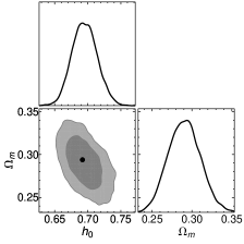
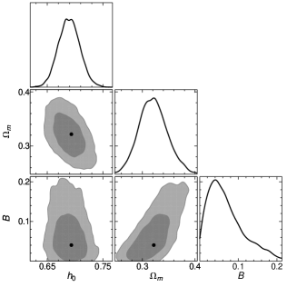
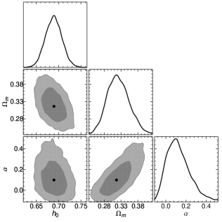
Figure 1: Contour plots and best-fit parameters (black dots) of $\Lambda$CDM (top left), GL1 (top right), GL2 (bottom left), and GCG (bottom right) models. Darker (lighter) areas mark $1$–$\sigma$ ($2$–$\sigma$) confidence regions.

Fig. 1 and Tab. 1 show, respectively, the contour plots and the best-fit parameters of the considered submodels. We indicated $H_{0}=100h_{0}$, and fixed $\Omega_{\rm r}=9.265\times 10^{-5}$ and $\Omega_{\rm b}=0.0493$ Planck Collaboration (2020).

With $N$ data, maximum log-likelihood $\ln\mathcal{L}$ and parameters $p$, for each proposed submodel we define the Aikake Information Criterion (AIC) and the Bayesian Information Criterion (BIC) Liddle (2007), respectively,

$${\rm AIC} =-2\ln\mathcal{L}+2p\,,$$ (28a)

$${\rm BIC} =-2\ln\mathcal{L}+p\ln N\,.$$ (28b)

The best-suited model provides the lowest values AIC₀ and BIC₀. The differences $\Delta={\rm AIC}-{\rm AIC}_{0}$ (${\rm BIC}-{\rm BIC}_{0}$) provide evidence against the proposed model as follows

• $\Delta\in[0,\,3]$, weak evidence;

• $\Delta\in(3,\,6]$, mild evidence;

• $\Delta>6$, strong evidence.

Immediately, Tab. 1 shows that $\Lambda$CDM and GL1 models are equally best suited, the GCG model is weakly disfavoured, and the GL2 model is mildly excluded. These results also enable constraints on the parameters ($\alpha$, $\rho_{\star}$, $A_{\star}$).

• $\Lambda$CDM. Assuming $\alpha\gtrsim 0$, from Eqs. (10) we get

  $$A_{\star}=\frac{3H_{0}^{2}}{8\pi G}\left[\ln\left(\frac{8\pi G\rho_{\star}}{3H_{0}^{2}}\right)\right]^{-1}\left(1-\Omega_{\rm M}-\Omega_{\rm R}\right)\,,$$ (29)

  that is not enough to break the degeneracy between $\rho_{\star}$ and $A_{\star}$, unless we impose $\rho_{\star}\equiv\rho_{\rm P}$ as in Tab. 1.

• GL1 and GL2. Assuming $\alpha\gtrsim 0$, from Eqs. (13) we are now able to set conditions on both $\rho_{\star}$ and $A_{\star}$

  $$\rho_{\star}= \frac{3H_{0}^{2}\Omega_{\rm M}}{8\pi G}\exp\left(1+\frac{1}{B}\right)\,,$$ (30a)

  $$A_{\star}= \frac{3H_{0}^{2}B}{8\pi G}\left(1-\Omega_{\rm m}-\Omega_{\rm r}\right)\,.$$ (30b)

  For GL1 we evaluated only $A_{\star}$, since $\rho_{\star}\equiv\rho_{\rm P}$, while for GL2 we evaluated both $\rho_{\star}$ and $A_{\star}$ (see Tab. 1).

• GCG. Here $\alpha$ is a model parameter and its best-fit value, see Tab. 1, agrees with Ref. Zheng et al. (2022). However, from Eqs. (16) we obtain one condition only

  $$A_{\star}=\alpha\frac{A_{\rm s}}{\rho_{\star}^{\alpha}}\left(\frac{3H_{0}^{2}}{8\pi G}\right)^{1+\alpha}\left(1-\Omega_{\rm b}-\Omega_{\rm r}\right)^{1+\alpha}\,,$$ (31)

  that does not allow us to “disentangle” $\rho_{\star}$ and $A_{\star}$.

IV Physical interpretation

Some interesting physical consequences can be drawn from the above analyses.

• At $a\approx 1$, the Murnaghan EoS in Eq. (8) is approximated by the $\Lambda$CDM model for $\rho\approx\rho_{\rm c}$.

• GL1 is statistically identical to and degenerates with the $\Lambda$CDM model; GL2 is mildly excluded. As $\Lambda$CDM and GL1 models are limiting cases of Eq. (8), we deduce that the condition $\rho_{\star}\equiv\rho_{\rm P}$ holds also for the most general Murnaghan EoS, i.e., when no approximation holds.

• At $10^{-5}\lesssim a\lesssim 1$, for $\rho_{\star}\equiv\rho_{\rm P}$, the term $(\rho_{\rm P}/\rho)^{\alpha}$ dominates and Eq. (8) is approximated by the GCG model, which is the only framework able to get constraints on $\alpha$ (see Tab. 1).

• Using the constraints on $\rho_{\star}\equiv\rho_{\rm P}$ (from $\Lambda$CDM and GL1 submodels) and $\alpha$ (from the GCG model), from Eq. (31) we get the value of $A_{\star}$ for the GCG case (see Tab. 1) that also holds for the total Murnaghan EoS.

• At early times, when $a\approx 0$ and $x=\rho_{\rm P}/\rho\approx 1$, at the lowest order we have $x^{\alpha}-1\approx\ln x^{\alpha}$, thus, Eq. (8) reduces to the GL1 model, as in Eq. (12).

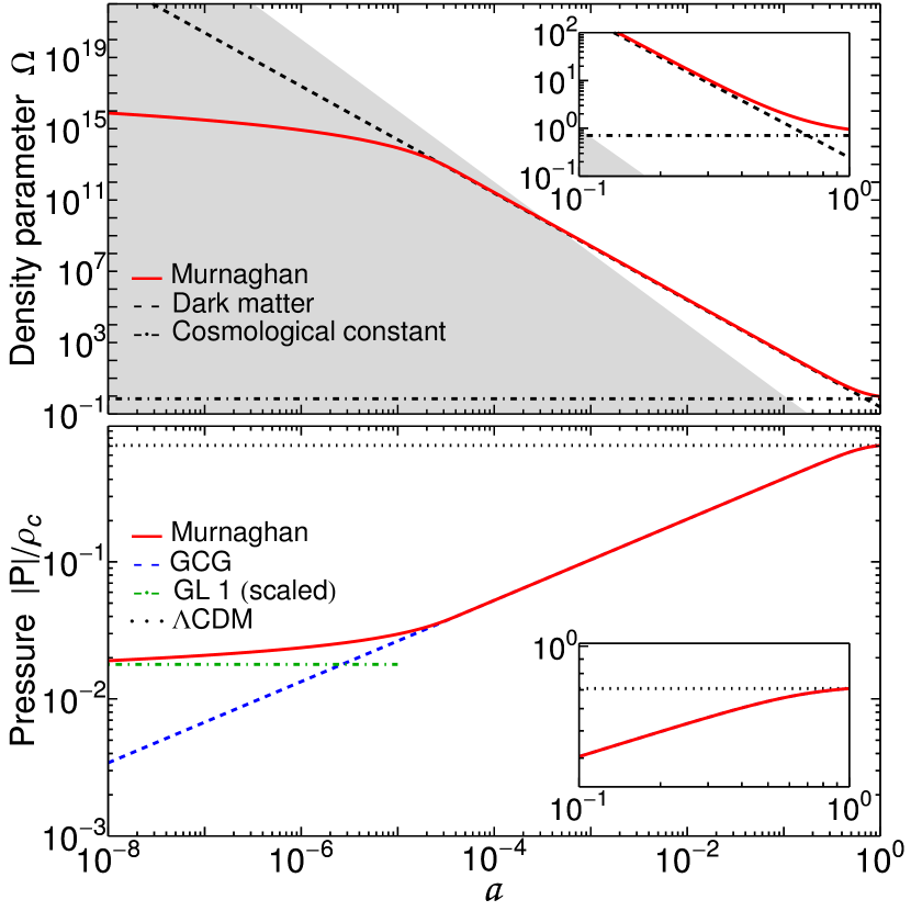
Figure 2: Top panel: Murnaghan density compared to $\Lambda$CDM dark matter, dark energy, and radiation (shaded area) ones. Bottom panel: comparison among Murnaghan, GCG, GL1 (rescaled to Murnaghan as $a\rightarrow 0$), and $\Lambda$CDM EoSs. The insets focus on $0.1\leq a\leq 1$. Parameters are taken from Tab. 1.

In view of the above considerations, we fix the following viable bounds:

$$\bar{\alpha} =0.10^{+0.18}_{-0.15}\,,$$ (32a)

$$\bar{\rho}_{\star} =\rho_{\rm P}\,,$$ (32b)

$$\bar{A}_{\star} =\left(5.31^{+0.48}_{-0.48}\right)\times 10^{-14}\rho_{\rm c}\,,$$ (32c)

which can be considered as “average quantities” obtained from the limiting cases at different times.

The corresponding best-fit cosmological parameters, with associated errors, can be found from the numerical bounds obtained from $\Lambda$CDM, GL1 and GCG models:

$$\bar{h}_{0} =0.692^{+0.030}_{-0.029}\,,$$ (33a)

$$\bar{\Omega}_{\rm M} =0.301^{+0.069}_{-0.041}\,.$$ (33b)

The above model ($\bar{\alpha}$, $\bar{\rho}_{\star}$, $\bar{A}_{\star}$) and cosmological ($\bar{h}_{0}$, $\bar{\Omega}_{\rm m}$) parameters have been used to obtain the numerical density displayed in the top panel of Fig. 2. The comparison among Murnaghan, GCG, GL1 (rescaled to Murnaghan as $a\rightarrow 0$) and $\Lambda$CDM scenarios is portrayed in the bottom panel of Fig. 2. These curves show explicitly the behavior of the full numerical solution and enable us to summarize our physical interpretation as follows.

• At early times, or $a\lesssim 10^{-5}$, the model acts as a logotropic fluid that degenerates with the $\Lambda$CDM model. Thus, in our framework we expect that structure formation proceeds with a behaviour similar to the current standard cosmological model.

• At $10^{-5}\lesssim a\lesssim 1$, the model acts as a GCG solution and agrees with late time observations.

• In the current epoch, or at $a\approx 1$, the model behaves again as GL1 or $\Lambda$CDM models.

Thus, the overall model appears to extend both logotropic and GCG scenarios, quite agreeing with observations, explaining in which regions of the Universe evolution the $\Lambda$CDM model is recovered and, consequently, fixing the coincidence issue between $\Omega_{\Lambda}$ and $\Omega_{{\rm m}}$.

To disclose the impact on structure formation, we analyze below how our model acts over linear perturbations.

V Impact on linear perturbations

The basic expressions used to describe structure formation in the Universe are the continuity and Euler equations, respectively given by

$$\delta^{\prime}+3(s-w)\delta+(1+w)\tilde{\theta} =0,$$ (34a)

$$\tilde{\theta}^{\prime}+\left(2+\frac{H^{\prime}}{H}\right)\tilde{\theta}+\frac{3}{2}(1+3s)\Omega(a)\delta =0,$$ (34b)

where we defined $\tilde{\theta}=\theta/H$ and introduced the divergence $\theta$ of the peculiar velocity $\mathbf{u}$, such that $\theta=\vec{\nabla}\cdot\mathbf{u}$. All the other quantities involved in the above equations are already defined by Eqs. (22) in Section III.

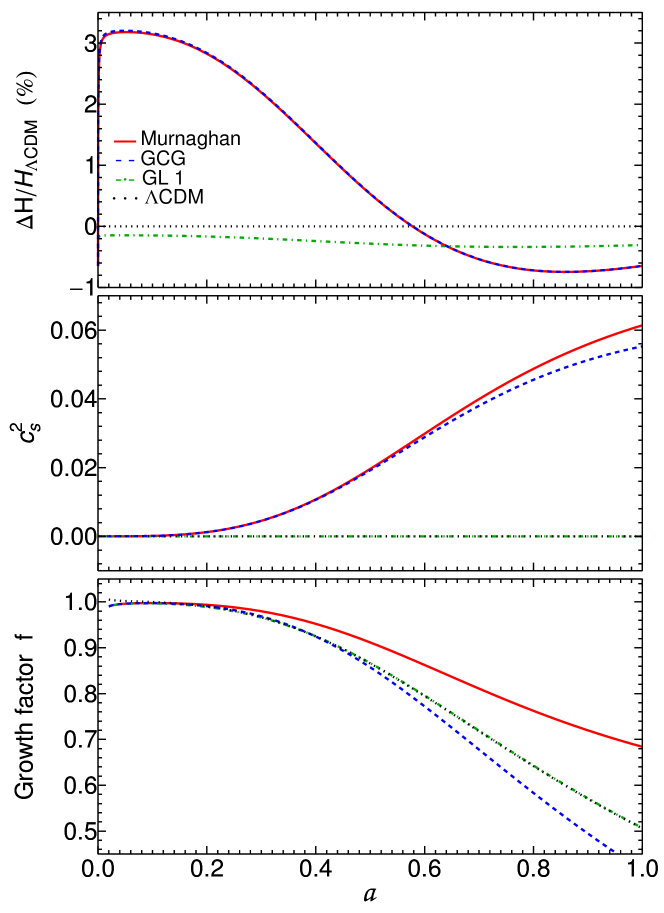
Figure 3: Murnaghan, GCG, GL1, and $\Lambda$CDM models comparison. Top panel: Hubble rate relative differences with respect to the $\Lambda$CDM one. Middle panel: squared sound speeds. Bottom panel: growth factors. Parameters are taken from Tab. 1.

By taking the derivative of Eq. (34a) and substituting it in Eq. (34b) we derive Eq. (21) and then Eq. (23), that can be solved following the standard assumptions listed below Boshkayev et al. (2021).

• The dark matter is the clustering component, so one can set $w=0$.

• With the phenomenological solution $f\approx\Omega_{\rm m}^{\gamma}(a)$ (Paul and Thakur, 2013), we obtain a first-order differential equation for $\gamma$ which is linearized by assuming $\Omega_{\rm m}\approx\mathcal{O}(1)$.

• The sound speed vanishes, so one can set $s=0$.

However, in our model we have the advantage to just consider the first assumption above and proceed with the numerical evaluations for $\Lambda$CDM, GL1, GCG approximations and Murnaghan model, we obtain the evolution of the Hubble parameter in Fig. 3 (top panel), portrayed as the relative departure with respect to the reference $\Lambda$CDM model that never exceeds the $\approx 3\%$ error for $0\leq a\leq 1$. The evolution of the adiabatic sound speed, which determines the stability and the validity of a given model against perturbations, is shown in Fig. 3 (middle panel). The evolution of the growth factor $f$ is shown in the bottom panel of Fig. 3. The parameters used in the plots are taken from Tab. 1 whereas the parameters for the Murnaghan model are taken from Eqs. (32)–(33).

Our main results are thus listed in the following.

• All the models have negligible, positive and real sound speeds (identically zero only for the $\Lambda$CDM model).

• At very early times, for all models, $f$ flattens to a value $\approx 1$, as expected, then decreases.

• At late times, the GCG (GL1) model departs from (degenerates with) the $\Lambda$CDM one due to its non-zero, albeit extremely small, sound speed.

• Our model largely deviates from the $\Lambda$CDM scenario, resulting in a more efficient growth of perturbations. This cannot be explained by the sound speed, similar to that of the GCG model (see the middle panel of Fig. 3), but rather depends on the density parameter of the perturbed fluid $\Omega(a)$, that accounts for the total dark fluid density enhancing the growth of perturbations.

Hence, our model, that employs the novel concept of matter with non-zero pressure, seems to better behave than the standard $\Lambda$ model alone, showing how dark energy can change its functional behaviours throughout the entire Universe evolution.

VI Conclusions

We are currently witnessing increased interest in unified dark energy models, aiming to explain cosmic acceleration using a single matter fluid exhibiting varying properties at different stages of the Universe’s evolution. Within this context, we propose employing a double polytropic EoS, consisting of two adiabatic indexes, one set to zero, while the other is negative. This approach allows us to replicate the effects of a specific EoS, resembling a combination of a Chaplygin gas fluid and a non-zero cosmological constant contribution. However, this combination seems finely tuned and compatible with the bare cosmological constant value, but not with quantum fluctuations. In this regard, we showed the fluid exhibits similarities to the Murnaghan EoS, a widely-used relation in solid state physics, particularly in describing pressure regimes within crystals.

The Murnaghan EoS is therefore here introduced in cosmological contexts. In particular, we showed that it reduces to the pure $\Lambda$CDM, logotropic and GCG cases, depending on the choices of $\rho$. This interesting property is a crucial feature of our model, showing that it represents a unified dark energy framework that at the same time, unifies the phenomenological descriptions of different dark energy models into one single fluid of matter with non-zero pressure, found in physical contexts and applied to the observable Universe.

We considered characteristics during the background cosmological regime and at early times, conducting a thorough investigation that encompassed cosmological observations involving SNe Ia, OHD, matter growth factor and $\sigma_{8}$ data. Our emphasis is centered on structure formation, with a specific focus on first-order perturbation theory.

We found that our model presents an intriguing prospect, with improved behavior when compared to the $\Lambda$CDM model, which uniformly assumes a vanishing sound speed for perturbations. In contrast, our model introduces a non-zero cutoff contingent upon the density scale. This particular attribute prompts an exploration into whether galaxies could potentially form even earlier than standard expectations, partially in line with recent developments recently discussed by the James Webb Telescope Arrabal Haro et al. (2023).

Future work will concentrate on more intricate applications of the Murnaghan EoS, incorporating self-interacting fluids. As demonstrated in Ref. Dunsby et al. (2024), it is plausible to interpret this fluid through a scalar field description, leading to a symmetry-breaking potential that contributes to the constant term evident in the Murnaghan EoS. Consequently, the incorporation of more complex versions of the potential itself will offer insights into potential refinements of our current model, positioning it as a robust alternative to prior unified dark energy models.

References

- Perlmutter et al. (1998) S. Perlmutter, G. Aldering, M. della Valle, S. Deustua, R. S. Ellis, S. Fabbro, A. Fruchter, G. Goldhaber, D. E. Groom, I. M. Hook, et al., Nature 391, 51 (1998), eprint astro-ph/9712212.
- Riess et al. (1998) A. G. Riess, A. V. Filippenko, P. Challis, A. Clocchiatti, A. Diercks, P. M. Garnavich, R. L. Gilliland, C. J. Hogan, S. Jha, R. P. Kirshner, et al., AJ 116, 1009 (1998), eprint astro-ph/9805201.
- Perlmutter et al. (1999) S. Perlmutter, G. Aldering, G. Goldhaber, R. A. Knop, P. Nugent, P. G. Castro, S. Deustua, S. Fabbro, A. Goobar, D. E. Groom, et al., ApJ 517, 565 (1999), eprint astro-ph/9812133.
- Tonry et al. (2003) J. L. Tonry, B. P. Schmidt, B. Barris, P. Cand ia, P. Challis, A. Clocchiatti, A. L. Coil, A. V. Filippenko, P. Garnavich, C. Hogan, et al., ApJ 594, 1 (2003), eprint astro-ph/0305008.
- Bridle et al. (2003) S. L. Bridle, O. Lahav, J. P. Ostriker, and P. J. Steinhardt, Science 299, 1532 (2003), eprint astro-ph/0303180.
- Bennett et al. (2003) C. L. Bennett, M. Halpern, G. Hinshaw, N. Jarosik, A. Kogut, M. Limon, S. S. Meyer, L. Page, D. N. Spergel, G. S. Tucker, et al., ApJ Suppl. Ser. 148, 1 (2003), eprint astro-ph/0302207.
- Hinshaw et al. (2003) G. Hinshaw, D. N. Spergel, L. Verde, R. S. Hill, S. S. Meyer, C. Barnes, C. L. Bennett, M. Halpern, N. Jarosik, A. Kogut, et al., ApJ Suppl. Ser. 148, 135 (2003), eprint astro-ph/0302217.
- Kogut et al. (2003) A. Kogut, D. N. Spergel, C. Barnes, C. L. Bennett, M. Halpern, G. Hinshaw, N. Jarosik, M. Limon, S. S. Meyer, L. Page, et al., ApJ Suppl. Ser. 148, 161 (2003), eprint astro-ph/0302213.
- Spergel et al. (2003) D. N. Spergel, L. Verde, H. V. Peiris, E. Komatsu, M. R. Nolta, C. L. Bennett, M. Halpern, G. Hinshaw, N. Jarosik, A. Kogut, et al., ApJ Suppl. Ser. 148, 175 (2003), eprint astro-ph/0302209.
- Eisenstein et al. (2005) D. J. Eisenstein, I. Zehavi, D. W. Hogg, R. Scoccimarro, M. R. Blanton, R. C. Nichol, R. Scranton, H.-J. Seo, M. Tegmark, Z. Zheng, et al., ApJ 633, 560 (2005), eprint astro-ph/0501171.
- Sahni and Starobinsky (2000) V. Sahni and A. Starobinsky, International Journal of Modern Physics D 9, 373 (2000), eprint astro-ph/9904398.
- Copeland et al. (2006) E. J. Copeland, M. Sami, and S. Tsujikawa, International Journal of Modern Physics D 15, 1753 (2006), eprint hep-th/0603057.
- Tsujikawa (2011) S. Tsujikawa, in Astrophysics and Space Science Library, edited by S. Matarrese, M. Colpi, V. Gorini, and U. Moschella (2011), vol. 370 of Astrophysics and Space Science Library, p. 331, eprint 1004.1493.
- Maia et al. (2009) M. D. Maia, A. J. S. Capistrano, and E. M. Monte, International Journal of Modern Physics A 24, 1545 (2009), eprint 0905.3655.
- Bamba et al. (2012) K. Bamba, S. Capozziello, S. Nojiri, and S. D. Odintsov, Astrophysics and Space Science 342, 155 (2012), eprint 1205.3421.
- Padmanabhan (2003) T. Padmanabhan, Phys. Rep. 380, 235 (2003), eprint hep-th/0212290.
- Peebles and Ratra (2003) P. J. Peebles and B. Ratra, Reviews of Modern Physics 75, 559 (2003), eprint astro-ph/0207347.
- Luongo and Quevedo (2014) O. Luongo and H. Quevedo, Phys. Rev. D 90, 084032 (2014), eprint 1407.1530.
- Giambò et al. (2020) R. Giambò, O. Luongo, and H. Quevedo, Phys. Dark Univ. 30, 100721 (2020), eprint 2010.05061.
- Luongo et al. (2024) O. Luongo, H. Quevedo, and S. N. Sajadi, Gen. Rel. Grav. 56, 17 (2024), eprint 2311.13264.
- Luongo and Quevedo (2023) O. Luongo and H. Quevedo (2023), eprint 2305.11185.
- Capozziello et al. (2013) S. Capozziello, M. De Laurentis, O. Luongo, and A. Ruggeri, Galaxies 1, 216 (2013), eprint 1312.1825.
- Linder and Scherrer (2009) E. V. Linder and R. J. Scherrer, Phys. Rev. D 80, 023008 (2009), eprint 0811.2797.
- Perković and Štefančić (2020) D. Perković and H. Štefančić, European Physical Journal C 80, 629 (2020), eprint 2004.05342.
- Bagla et al. (2003) J. S. Bagla, H. K. Jassal, and T. Padmanabhan, Phys. Rev. D 67, 063504 (2003), eprint astro-ph/0212198.
- Schmidt (2007) H.-J. Schmidt, International Journal of Geometric Methods in Modern Physics 04, 209 (2007), eprint gr-qc/0602017.
- Nojiri et al. (2017) S. Nojiri, S. D. Odintsov, and V. K. Oikonomou, Phys. Rep. 692, 1 (2017), eprint 1705.11098.
- Luongo and Quevedo (2018) O. Luongo and H. Quevedo, Foundations of Physics 48, 17 (2018).
- Bamba et al. (2013) K. Bamba, R. Gannouji, M. Kamijo, S. Nojiri, and M. Sami, JCAP 2013, 017 (2013), eprint 1211.2289.
- Weinberg (1989) S. Weinberg, Reviews of Modern Physics 61, 1 (1989).
- Luongo and Muccino (2018) O. Luongo and M. Muccino, Phys. Rev. D 98, 103520 (2018), eprint 1807.00180.
- Gruber and Luongo (2014) C. Gruber and O. Luongo, Phys. Rev. D 89, 103506 (2014), eprint 1309.3215.
- del Campo et al. (2012) S. del Campo, I. Duran, R. Herrera, and D. Pavón, Three thermodynamically based parametrizations of the deceleration parameter (2012), eprint 1209.3415.
- Arbey and Mahmoudi (2021) A. Arbey and F. Mahmoudi, Progress in Particle and Nuclear Physics 119, 103865 (2021), eprint 2104.11488.
- Profumo et al. (2019) S. Profumo, L. Giani, and O. F. Piattella, Universe 5, 213 (2019), eprint 1910.05610.
- Capozziello et al. (2018) S. Capozziello, O. Luongo, R. Pincak, and A. Ravanpak, Gen. Rel. Grav. 50, 53 (2018), eprint 1804.03649.
- Belfiglio and Luongo (2024) A. Belfiglio and O. Luongo (2024), eprint 2401.16910.
- Luongo and Mengoni (2023) O. Luongo and T. Mengoni (2023), eprint 2309.03065.
- Belfiglio et al. (2023a) A. Belfiglio, O. Luongo, and S. Mancini (2023a), eprint 2312.11419.
- Belfiglio et al. (2023b) A. Belfiglio, Y. Carloni, and O. Luongo (2023b), eprint 2307.04739.
- Belfiglio et al. (2023c) A. Belfiglio, O. Luongo, and S. Mancini, Phys. Rev. D 107, 103512 (2023c), eprint 2212.06448.
- Belfiglio et al. (2022) A. Belfiglio, O. Luongo, and S. Mancini, Phys. Rev. D 105, 123523 (2022), eprint 2201.12299.
- Pérez de los Heros (2020) C. Pérez de los Heros, Symmetry 12, 1648 (2020), eprint 2008.11561.
- Avelino et al. (2008) P. P. Avelino, L. M. G. Beça, and C. J. A. P. Martins, Phys. Rev. D 77, 063515 (2008), eprint 0711.4288.
- Beça and Avelino (2007) L. M. G. Beça and P. P. Avelino, MNRAS 376, 1169 (2007), eprint astro-ph/0507075.
- Bento and Bertolami (1999) M. C. Bento and O. Bertolami, General Relativity and Gravitation 31, 1461 (1999), eprint gr-qc/9905075.
- Hu and Eisenstein (1999) W. Hu and D. J. Eisenstein, Phys. Rev. D 59, 083509 (1999), eprint astro-ph/9809368.
- Aviles and Cervantes-Cota (2011) A. Aviles and J. L. Cervantes-Cota, Phys. Rev. D 84, 089905 (2011), eprint 1108.2457.
- Chavanis (2015) P.-H. Chavanis, European Physical Journal Plus 130, 130 (2015), eprint 1504.08355.
- Fabris et al. (2011) J. C. Fabris, H. E. S. Velten, C. Ogouyandjou, and J. Tossa, Physics Letters B 694, 289 (2011), eprint 1007.1011.
- Luongo and Quevedo (2014) O. Luongo and H. Quevedo, International Journal of Modern Physics D 23, 1450012 (2014).
- Boshkayev et al. (2021) K. Boshkayev, T. Konysbayev, O. Luongo, M. Muccino, and F. Pace, Phys. Rev. D 104, 023520 (2021), eprint 2103.07252.
- Dunsby et al. (2024) P. K. S. Dunsby, O. Luongo, and M. Muccino, Phys. Rev. D 109, 023510 (2024), eprint 2308.15776.
- Bento et al. (2002) M. C. Bento, O. Bertolami, and A. A. Sen, Phys. Rev. D 66, 043507 (2002), eprint gr-qc/0202064.
- Murnaghan (1944a) F. D. Murnaghan, Proceedings of the National Academy of Science 30, 244 (1944a).
- Moresco et al. (2022) M. Moresco, L. Amati, L. Amendola, S. Birrer, J. P. Blakeslee, M. Cantiello, A. Cimatti, J. Darling, M. Della Valle, M. Fishbach, et al., Living Reviews in Relativity 25, 6 (2022), eprint 2201.07241.
- Scolnic et al. (2018) D. M. Scolnic, D. O. Jones, A. Rest, Y. C. Pan, R. Chornock, R. J. Foley, M. E. Huber, R. Kessler, G. Narayan, A. G. Riess, et al., ApJ 859, 101 (2018), eprint 1710.00845.
- Paul and Thakur (2013) B. C. Paul and P. Thakur, JCAP 2013, 052 (2013), eprint 1306.4808.
- Muccino et al. (2021) M. Muccino, L. Izzo, O. Luongo, K. Boshkayev, L. Amati, M. Della Valle, G. B. Pisani, and E. Zaninoni, Astrophys. J. 908, 181 (2021), eprint 2012.03392.
- Dunsby et al. (2016) P. K. S. Dunsby, O. Luongo, and L. Reverberi, Phys. Rev. D 94, 083525 (2016), eprint 1604.06908.
- Martin (2012) J. Martin, Comptes Rendus Physique 13, 566 (2012), eprint 1205.3365.
- Murnaghan (1944b) F. D. Murnaghan, Proceedings of the National Academy of Science 30, 244 (1944b).
- Chavanis (2016) P.-H. Chavanis, Physics Letters B 758, 59 (2016), eprint 1505.00034.
- Zheng et al. (2022) J. Zheng, S. Cao, Y. Lian, T. Liu, Y. Liu, and Z.-H. Zhu, European Physical Journal C 82, 582 (2022), eprint 2208.06167.
- Jimenez and Loeb (2002) R. Jimenez and A. Loeb, ApJ 573, 37 (2002), eprint astro-ph/0106145.
- Riess et al. (2018) A. G. Riess, S. A. Rodney, D. M. Scolnic, D. L. Shafer, L.-G. Strolger, H. C. Ferguson, M. Postman, O. Graur, D. Maoz, S. W. Jha, et al., ApJ 853, 126 (2018), eprint 1710.00844.
- Weinberg (1972) S. Weinberg, Gravitation and Cosmology: Principles and Applications of the General Theory of Relativity (1972).
- Planck Collaboration (2020) Planck Collaboration, A&A 641, A6 (2020), eprint 1807.06209.
- Liddle (2007) A. R. Liddle, MNRAS 377, L74 (2007), eprint astro-ph/0701113.
- Arrabal Haro et al. (2023) P. Arrabal Haro, M. Dickinson, S. L. Finkelstein, J. S. Kartaltepe, C. T. Donnan, D. Burgarella, A. C. Carnall, F. Cullen, J. S. Dunlop, V. Fernández, et al., Nature 622, 707 (2023), eprint 2303.15431.