Optimal Euclidean Tree Covers
Abstract
A -stretch tree cover of a metric space is a collection of trees, where every pair of points has a -stretch path in one of the trees. The celebrated Dumbbell Theorem [Arya et al. STOC’95] states that any set of points in -dimensional Euclidean space admits a -stretch tree cover with trees, where the notation suppresses terms that depend solely on the dimension . The running time of their construction is . Since the same point may occur in multiple levels of the tree, the maximum degree of a point in the tree cover may be as large as , where is the aspect ratio of the input point set.
In this work we present a -stretch tree cover with trees, which is optimal (up to the factor). Moreover, the maximum degree of points in any tree is an absolute constant for any . As a direct corollary, we obtain an optimal routing scheme in low-dimensional Euclidean spaces. We also present a -stretch Steiner tree cover (that may use Steiner points) with trees, which too is optimal. The running time of our two constructions is linear in the number of edges in the respective tree covers, ignoring an additive term; this improves over the running time underlying the Dumbbell Theorem.
1 Introduction
Let be a given metric space with distance function , and be a finite set of points in . A tree cover for is a collection of trees , each of which consists of (only) points in as vertices and abstract edges between vertices, such that between every two points and in , for every tree in . A tree cover has stretch if for every two points and in , there is a tree in that preserves the distance between and up to factor: . We call such an -tree cover of . In this paper, we will focus on the scenario where is the -dimensional Euclidean space for some constant . It is not hard to see that, in this case, the edges can be drawn as line segments in between the corresponding two endpoints, with weights equal to their Euclidean distances. If we relax the condition so that trees in may have other points from (called Steiner points) as vertices instead of just points from , the resulting tree cover is called a Steiner tree cover.
Constructions of tree covers, due to their algorithmic significance, are subject to growing research attention [AP92, AKPW95, ADM+95, GKR01, MN06, DYL06, CGMZ16, BFN22, CCL+23a, CCL+23b]; by now generalizations in various metric spaces and graphs are well-explored. The main measure of quality for tree cover is its size, that is, the number of trees in a tree cover . The existence of a small tree cover provides a framework to solve distance-related problems by essentially reducing them to trees. Exemplified applications include distance oracles [CCL+23a, CCL+23b], labeling and routing schemes [TZ05, KLMS22], spanners with small hop diameters [KLMS22], and bipartite matching [ACRX22].
The celebrated Dumbbell Theorem by Arya, Das, Mount, Salowe, and Smid [ADM+95] from almost thirty years ago demonstrated that in -dimensional Euclidean space, any point set has a tree cover of stretch that uses only trees.111The notation suppresses terms that depend solely on the dimension . Moreover, the tree cover can be computed within time , where is the number of points in . In the Euclidean plane (when ), this gives us a tree cover of size . The theorem has a long and complex proof, which spans a chapter in the book of Narasimhan and Smid [NS07]. A few years ago, this theorem was generalized for doubling metrics222the doubling dimension of a metric space is the smallest value such that every ball in can be covered by balls of half the radius; a metric is called doubling if its doubling dimension is constant by Bartal, Fandina, and Neiman [BFN22], who achieved the same bound as [ADM+95] via a much simpler construction; the running time of their construction was not analyzed.333In high-dimensional Euclidean spaces the upper bound in [BFN22] improves over that of [ADM+95], since the notation in [ADM+95] and [BFN22] suppress multiplicative factors of and , respectively. In the constructions by [ADM+95, BFN22], same point may have multiple copies in different levels of the tree, hence the maximum degree of points444the degree of a point is the number of edges incident to it may be as large as , where is the aspect ratio of the input point set; see Sections 1.3 and 4 for a more detailed discussion.
Since the number of trees provided by the two known constructions [ADM+95, BFN22] matches the packing bound -d (up to a logarithmic factor), it is tempting to conjecture that this bound is tight. However, there is a gap between this upper bound and the best lower bound we have, which comes indirectly from -stretch spanners. For any parameter , a Euclidean -spanner for any -dimensional point set is a weighted graph spanning the input point set, whose edge weights are given by the Euclidean distances between the points, that approximates all the original pairwise Euclidean distances within a factor of . We note that an -spanner can be obtained directly by taking the union of all trees in any -tree cover for the input point set. The size lower bound for -spanners [LS22, Theorem 1.1] directly implies that any -tree cover must contain trees. This is an -1-factor away from the packing bound. In particular, in the Euclidean plane, there is a gap between the upper bound of and the lower bound of . One can extend the notions of spanner by introducing Steiner points as well, which are additional points that are not part of the input. A weaker lower bound can be obtained for Steiner tree cover, from the size lower bound for Steiner -spanner in [LS22, Theorem 1.4], and the size lower bound in general [BT22].
1.1 Short Survey on Tree Covers
There are many papers published on tree covers in recent years, with subtle variations in their definitions due to differences in main objectives and applications. Here we attempt to summarize the best upper and lower bounds known to our knowledge, highlighting the tradeoff between tree cover size and stretch in the previous work. Some of the bounds are not explicitly stated in the cited reference but can be deduced from it. For additional relevant work, refer to [BFN22] and the references therein.
General metrics.
The earliest literature on the notion of tree cover is probably Awerbuch and Peleg [AP92] and Awerbuch, Kutten, and Peleg [AKP94], focusing on graph metrics. Their main objective is to minimize the number of trees each vertex belongs to (in the sparse cover sense) instead of minimize the total number of trees. Thorup and Zwick [TZ05, Corollary 4.4] improved over Awerbuch and Peleg [AP92] by constructing a Steiner tree cover with stretch where every vertex belongs to trees. Charikar et al. [CCG+98] studies a similar problem of probabilistically embedding finite metric space into a small number of trees. Many of the earlier work on tree covers are motivated by application in routing [TZ01a].
Gupta, Kumar, and Rastogi [GKR01, Theorem 4.3] observed that any tree cover must have size if the stretch is ; the lower bound is based on the existence of girth- graphs with edges [Mar88][ADD+93, Lemma 9]. It is important to emphasize that the tree covers considered in [GKR01] are spanning — the trees must be subgraphs of the input graph. Bartal, Fandina, and Neiman established the same lower bound [BFN22, Corollary 13] by reduction from spanners [ADD+93]. In a different direction, Dragan, Yan, and Lomonosov [DYL06] studied spanner tree covers with additive stretch on special classes of graphs, such as chordal graphs and co-comparability graphs.
One might relax the condition to allow vertices not presented in the graph (called Steiner vertices) to be part of the tree cover. By allowing Steiner vertices, Mendel and Naor [MN06] showed that any -point metric space has a Steiner tree cover of size and stretch . Bartal, Fandina, and Neiman [BFN22] obtained an inverse tradeoff: any -point metric space has a Steiner tree cover of size and stretch . In particular, this means we can get trees with stretch. While the lower bound from [GKR01] for spanning tree cover no longer holds when Steiner vertices are allowed, a similar lower bound of for the size of Steiner -tree covers can be derived from Steiner spanners (also known as emulators) [ADD+93, Theorem 6], using the same argument in [BFN22].
Doubling metrics.
Chan, Gupta, Maggs, and Zhou [CGMZ16, Lemma 3.4] constructs Steiner tree covers for doubling metrics [CGMZ16]. More precisely, if the doubling dimension of the metric space is , their tree cover uses Steiner trees and has stretch . Bartal, Fandina, and Neiman [BFN22] obtained two separated constructions: one may have tree cover of stretch and Steiner trees for any [BFN22, Theorem 7] using the -padded hierarchical partition family in [ABN11, Lemma 8], or alternatively a tree cover with stretch and trees [BFN22, Theorem 3] using net trees. It is worth emphasizing that the second construction does not use Steiner points. They also established a lower bound on the size of non-Steiner tree cover [BFN22, Corollary 13] by reduction from spanners [ADD+93]: there is an -point metric space with doubling dimension , such that any -tree cover requires trees.
Planar and minor-free graphs.
On planar graphs Gupta, Kumar, and Rastogi [GKR01] constructed the first -size (non-Steiner) tree cover with stretch . Again this is improved by Bartal, Fandina, and Neiman in two different directions: either one has stretch and trees [BFN22, Corollary 9] using the -padded hierarchical partition family in [KLMN05]555the constants in [KLMN05] imply that the stretch is at least and the number of trees is at least , or alternatively a tree cover with stretch and trees [BFN22, Theorem 5], using path separators [AG06]. Their results naturally extend to minor-free graphs. Recently, the authors get the best of both worlds by constructing a Steiner tree cover with stretch using many trees [CCL+23a] through the introduction of a new graph partitioning scheme called the shortcut partition; the result also extends to minor-free graphs [CCL+23b].
On planar graphs trees are required if no stretch is allowed [GKR01]. However in the -stretch regime, we are not aware of any existing lower bounds. The strongest lower bound for tree covers on planar graphs we managed to deduce comes from distance labeling: Suppose we have a Steiner -tree cover using many trees for some . Then we can construct an approximate distance labeling scheme by concatenating the -length labeling schemes for all trees [FGNW17]. By setting , we get an exact labeling scheme for unweighted planar graph of length , contradicting to an information-theoretical lower bound [GPPR04]. This implies that any Steiner -tree covers on planar graphs requires at least many trees.
Euclidean metrics.
We already discussed tree cover results on Euclidean metrics in the introduction; here we mentioned a few additional facts.
All upper bound constructions on metrics with bounded doubling dimensions immediately apply to Euclidean metrics as well. Surprisingly, relatively few lower bounds have been established in the literature for Euclidean spaces. Early in the introduction we derived an lower bound for non-Steiner tree cover and an lower bound for Steiner tree cover in by reduction from spanners.
One thing to notice is that in Euclidean spaces, the meaning of Steiner points differs slightly from its graph counterparts: after choosing a Steiner point (which lies in the ambient space ), the weight of an edge incident to a Steiner point is determined by its Euclidean distance, unlike in the graph setting one may choose the weight freely (as the Steiner points are artificially inserted and were not part of the graph a priori). One might think that such a distinction cannot possibly make any difference; however, recently Andoni and Zhang [AZ23] proved that -spanner of subquadratic size exists for arbitrary dimensional Euclidean space by allowing out-of-nowhere Steiner points, while establishing lower bound simultaneously when the Steiner points are required to sit in the Euclidean space. They showed that there are points in (for some highe dimension depending on ) where any -spanner (with Euclidean Steiner points) requires edges; the lower bound follows from a randomized construction and volume argument. This translates to an almost linear lower bound ( on the minimum number of trees required in any Euclidean Steiner tree cover with stretch. All Steiner points used in our construction are Euclidean; at the moment, we are unaware of any tree cover construction that obtains a better bound by taking advantage of the non-Euclidean Steiner points.
Ramsey trees.
A stronger notion called the Ramsey tree cover has been studied, where every vertex is associated with a tree in , such that the distance from to every other vertex is approximated preserved by the same tree . Both the constructions of Mendel and Naor [MN06] and Bartal, Fandina, and Neiman [BFN22] for general metrics are indeed Ramsey trees. These bounds are essentially tight if the trees are required to be Ramsey; that is, any Ramsey tree cover of stretch must contain many tree [BFN22, Corollary 13]. Even when the input metric is planar and doubling, any Ramsey tree cover of stretch must contain many tree [BFN22, Theorem 10], and any Ramsey tree cover of size must has stretch [BFN22, Theorem 9].
1.2 Main Results
We improve the longstanding bound on the number of trees for Euclidean tree cover by a factor of , for any constant-dimensional Euclidean space.666As with [ADM+95], the notation in our bound suppresses a multiplicative factor of , which should be compared to the multiplicative factor of suppressed in the bound of [BFN22]. Thus, our results improve over that of [BFN22] only under the assumption that is sufficiently small with respect to the dimension ; this assumption should be acceptable since the focus of this work, as with the great majority of the work on Euclidean spanners, is low-dimensional Euclidean spaces. In view of the aforementioned lower bound [LS22, BT22], this is optimal up to the factor. Roughly speaking, we show that the packing bound barrier (incurred in both [ADM+95] and [BFN22]) can be replaced by the number of -angled cones needed to partition ; for more details, refer to Section 1.3.
Theorem 1.1
For every set of points in and any , there exists a tree cover with stretch and trees. The running time of the construction is .
We note our construction is faster than that of the Dumbbell Theorem of [ADM+95] by more than a multiplicative factor of -d.
In addition, we demonstrate that the bound on the number of trees can be quadratically improved using Steiner points; in we can construct a Steiner tree cover with stretch using only many trees. The result generalizes for higher dimensions. In view of the aforementioned lower bound [LS22, BT22], this result too is optimal up to the factor.
Theorem 1.2
For every set of points in and any , there exists a Steiner tree cover with stretch and trees. The running time of the construction is .
1.2.1 Bounded degree tree cover
Although the number of trees in the tree cover is the most basic quality measure, together with the stretch, another important measure is the degree. One can optimize the maximum degree of a point in any of the trees, or to optimize the maximum degree of a point over all trees — both these measures are of theoretical and practical importance.
Both the Dumbbell Theorem [ADM+95] and the BFN construction [BFN22] use copies of the same point in multiple trees, and even in different levels of the same tree. Consequently, each point may have up to copies, which can be viewed as distinct nodes of the tree, where is the aspect ratio of the input point set. The Dumbbell trees have bounded node-degree (which is improved to degree 3 in [Smi12]), but the maximum point-degree in any tree could still be after reidentifying all the copies of the points. The construction of [BFN22] may also incur a point-degree of in any of the trees.777Even node-degrees may blow up in the construction of [BFN22], but it appears that a simple tweak of their construction can guarantee a node-degree of -O(d).
We strengthen Theorem 1.1 by achieving a constant degree for each point in any of the trees; in fact, our bound is an absolute constant in any dimension. As a result, the maximum degree of a point over all trees is ; this is optimal up to the factor, matching the average degree (or size) lower bound of spanners mentioned above [LS22].
Routing.
We highlight one application of our bounded degree tree cover to efficient routing.
Theorem 1.3
For any set of points in and any , there is a compact routing scheme with stretch that uses routing tables and headers with bits of space.
Our routing scheme uses smaller routing tables compared to the routing scheme of Gottlieb and Roditty [GR08], which uses routing tables of bits. At a high level, we provide an efficient reduction from the problem of routing in low-dimensional Euclidean spaces to that in trees; more specifically, we present a new labeling scheme for determining the right tree to route on in the tree cover of Theorem 1.1. Having determined the right tree to route on, our entire routing algorithm is carried out on that tree, while the routing algorithm of [GR08] is carried out on a spanner; routing in a tree is clearly advantageous over routing in a spanner, also from a practical perspective. Refer to [GR08] for the definition of the problem and relevant background.
1.3 Technical Highlights
1.3.1 Achieving an optimal bound on the number of trees
The tree cover constructions of [ADM+95] and [BFN22] achieve the same bound of on the number of trees, which is basically the packing bound . The Euclidean construction of [ADM+95] is significantly more complex than the construction of [BFN22] that applies to the wider family of doubling metrics. Here we give a short overview of the simpler construction of [BFN22]; then we describe our Euclidean construction, aiming to focus on the geometric insights that we employed to breach the packing bound barrier.
The starting point of [BFN22] is the standard hierarchy of -nets {} [GKL03], which induces a hierarchical net-tree.888The standard notation in the literature on doubling metrics, including [BFN22], uses index instead of to refer to levels or distance scales; however, this paper focuses on Euclidean constructions, and we view it instructive to use a different notation. Each net is greedily partitioned into a collection of -sub-nets , which too are hierarchical. For a fixed level , the number of sub-nets is bounded by the packing bound , and each of them is handled by a different tree via a straightforward clustering procedure. Naïvely this introduces a factor to the number of trees, each corresponding to a level ( is the aspect ratio of the point set). The key observation to remove the dependency on the aspect ratio is that two far apart levels are more or less independent, and one can pretty much use the same collection of trees for both. More precisely, the levels are partitioned into congruence classes , where . Since distances across different levels of the same class differ by at least a factor of , it follows that all sub-nets can be handled by a single tree via a greedy hierarchical clustering. Now the total number of trees is the number of sub-nets in one level, which is , times the number of congruence classes .
Taking a bird’s eye view of the construction of [BFN22], the following two-step strategy is used to handle pairwise distances within each congruence class :
-
1.
Reduce the problem from the entire congruence class to a single level . This is done by a simple greedy procedure.
-
2.
Handle each level separately. This is done by a simple greedy clustering to the sub-nets .
In Euclidean spaces, we shall use quadtree which is the natural analog of the hierarchical net-tree. We too employ the trick of partitioning all levels in the hierarchy to congruence classes [CGMZ16, BFN22, LS22, ACRX22] and handle each one separately, and follow the above two-step strategy. However, the way we handle each of these two steps deviates significantly from [BFN22].
Step 1: Reduce the problem to a single level.
At any level , we handle every quadtree cell of width separately. Every cell is partitioned into subcells from level of width , and each non-empty cell contains a single representative assigned by the construction at level . At level , we construct a partial -tree cover, which roughly speaking only preserves distances between pairs of representatives that are at distance roughly from each other; this is made more precise in the description of Step 2 below. Let be the number of trees required for such a partial tree cover. To obtain a tree cover for all points in the current level- cell, we simply merge the aforementioned partial tree cover constructed for the level- representatives with the tree cover obtained previously for the points in the subcells. Finally, we choose one of those level- representatives as the level- representative of the current cell, and proceed to level of the construction.
To achieve the required stretch bound, it is sufficient to guarantee that for every pair of points , some quadtree cell of side-length proportional to would contain both and . Alas, this is impossible to achieve with a single quadtree. To overcome this obstacle, we use a result by Chan [Cha98]: there exists a collection of carefully chosen shifts of the input point set, such that in at least one shift there is a quadtree cell of side-length at most that contains both and . The number of trees in the cover grows by a factor of . Consequently, if each cell can be handled using trees, then ranging over all the congruence classes and all the shifts, the resulting tree cover consists of trees; see Lemma 2.4 for a more precise statement. The full details of the reduction are in Section 2.1.
Step 2: Handling a single level.
Handling a single level is arguably the more interesting step, since this is where we depart from the general packing bound argument that applies to doubling metrics, and instead employ a more fine-grained geometric argument. We next give a high-level description of the tree cover construction for a single level . For brevity, in this discussion we focus on the 2-dimensional construction that does not use Steiner points. The full details, as well as generalization for higher dimension and the Steiner tree cover construction, are given in Sections 2.2 and 2.3.
We consider a single 2-dimensional quadtree cell of side-length at level , which is subdivided into subcells of side-length . Every level- cell has a representative and our goal is to construct a partial tree cover for any pair of representatives that are at a distance between and . (The final constants are slightly different; here we choose 10 for simplicity.) To this end, we select a collection of directions. For each direction , we partition the plane into strips of width , each strip parallel to . We then shift each such partition orthogonally by ; we end up with a collection of partitions, two for each direction. We call these partitions the major strip partitions. Observe that for every pair of representative points and , there is at least one major strip partition in some direction, such that both and are contained in the same strip. Crucially, we show that for every strip in a partition , there is a collection of trees that preserves distances between all points and in strip that are at distance between and . The key observation is that, since the strips in the same partition are disjoint by design, the -many trees for each strip of can be combined into forests. Thus the total number of forests is .
To construct a collection of trees preserving distances within a single strip , we first subdivide the strip . If is in direction , we partition into sub-strips orthogonal to , each of width . We call this a minor strip partition. Observe that if points and are at distance , they are in different sub-strips of the minor strip partition. For every pair of sub-strips and in the minor strip partition, we construct a single tree that preserves distances between points in and to within a factor of . There are sub-strips in the minor strip partition, so overall only trees are needed for any strip .
1.3.2 Bounding the degree
The tree cover construction described above achieves the optimal bound on the number of trees, but the degree of points could be arbitrarily large. While the previous tree cover constructions [ADM+95, BFN22] incur unbounded degree, the Euclidean construction of [ADM+95], when restricted to a single level in the hierarchy, achieves an absolute constant degree.999Although in the original paper of [ADM+95] (as well as in [NS07]) the bound is not an absolute constant, it was shown in [Smi12] that an absolute constant bound can be obtained. Nonetheless, overlaying all levels of the hierarchy leads to a final degree bound of .
In our construction, when restricted to a single level, the degree of points can be easily bounded by . However, in contrast to [ADM+95], our goal is to achieve this bound for the entire tree, across all levels of the hierarchy. In particular, if we achieve this goal, the total degree of each point over all trees will be ( in general), which is optimal (up to logarithmic factor) due to the aforementioned lower bound [BT22]. To achieve this goal, we strengthen the aforementioned two-step strategy as follows.
Step 1.
In the reduction from the entire congruence class to a single level , the challenge is not to overload the same representative point over and over again across different levels of . To this end, we refine a degree reduction technique, originally introduced by Chan et al. [CGMZ16] to achieve a bounded degree for -stretch net-tree spanners in arbitrary doubling metrics. The technique of [CGMZ16] is applied on a bounded-arboricity net-tree spanner, first by orienting its edges to achieve bounded out-degree for all points. Then, apply a greedy edge-replacement process, where the edges are scanned in nondecreasing order of their level (or weight), and any incoming edge leading to a high-in-degree point is replaced by an edge leading to an incoming neighbor of in a sufficiently lower level, with . It is shown that this process terminates with a bounded-degree spanner, where the degree bound is quadratic in the out-degree bound (arboricity) of the original spanner, and the stretch bound increases only by an additive factor of .
We would like to apply this technique on every tree in the tree cover separately; if instead we were to apply it on the union of the trees, we would create cycles; resolving them blows up the number of trees in the cover. We demonstrate that by working on each tree separately, not only does the greedy edge-replacement process reduce the degree in each tree to an absolute constant, but it also keeps the tree cycle-free as well as provides the required stretch bound; see Section 4.1 for the details. In fact, it turns out to be advantageous to operate on each tree separately rather than on their union, since this way the out-degree bound in a single tree reduces to 1, which directly improves the total degree bound over all trees to be linearly depending on rather than quadratically. This is the key to achieving an optimal degree bound both within each tree as well as over all trees.
Step 2.
When handling a single level individually, the degree of points can be easily bounded by as mentioned. However, we would like to achieve an absolute constant bound at each level. Recall that, for every pair of sub-strips and in the minor strip partition of some strip , we construct a single tree that preserves distances between points in and to within a factor of ; this tree is in fact a star. Perhaps surprisingly, every such star can be transformed into a binary tree via a simple greedy procedure, with the stretch bound increased by just a factor of ; see Section 4.2 for the details.
1.4 Organization
In Section 2, we present the construction of tree covers in with an optimal number of trees in both non-Steiner and Steiner settings, proving Theorem 1.1 and Theorem 1.2 for the plane. In Section 3, we generalize these constructions to for arbitrary constant . In Section 4, we reduce the degree of every tree in the (non-Steiner) tree cover an absolute constant. In Section 5, we show some applications of our tree cover to routing, proving Theorem 1.3.
2 Optimal Tree Covers for Euclidean Spaces
2.1 Reduction to Partial Tree Cover
Let be a set of points in . For any two points and in , we use to denote their Euclidean distance. Without loss of generality we assume the minimum distance between any two points in is .
Lemma 2.1 (Cf. [Cha98, GH23])
Let be an arbitrary real parameter. Consider any two points , and let be the infinite quadtree of . For and , let . Then there exists an index , such that and are contained in a cell of with side-length at most .
Definition 2.2
We call two points -far if their distance is in .
Definition 2.3
A -partial tree cover for with stretch is a tree cover with the following property: for every two -far points and , there is a tree in the cover such that .
Lemma 2.4 (Reduction to partial tree cover)
Let be a set of points in , and let be a number in . Suppose that for every , every set of points in with diameter admits a -partial tree cover with stretch , size and diameter of each tree at most for some . Then admits a tree cover with stretch and size with .
-
Proof
Assume without loss of generality that the smallest coordinate of a point in is 0 and let be the largest coordinate in . Let and let be the quadtree as in Lemma 2.1. For , let be shifted by .
Constructing the tree cover. Let and let . (Assume for simplicity that is an integer.) Fix some , , and . We proceed to construct tree . Consider the congruence class . The following construction is done for every in increasing order. Consider the level- quadtree , with cells of width . If , for each level- cell , construct the th among trees from the -partial tree cover on the points in , and root it at an arbitrary point in . For , consider the subdivision of level- cell into subcells of level . Let be a subset of consisting of all the roots of the previously built subtrees in subcells of levels . Let , and observe that w is an upper-bound on the diameter of . Construct a -partial tree cover for with trees, and let be the th tree of the trees constructed. Take the previously built subtrees rooted at , and construct a new tree by identifying their roots with the vertices of . Root this new tree arbitrarily. The tree is the final tree obtained after iterating over every .
We prove the following two claims inductively.
Claim 2.5
Let be a tree constructed at level for , , and .
-
1.
is a tree.
-
2.
has diameter w at most .
-
1.
-
Proof
We prove the claim by induction over the level .
-
1.
The base case holds because the graph is initialized as a tree. For the induction step, consider some level that is at least . At this stage we construct a tree with vertex set consisting of representatives of the level , and attach the trees rooted at each of the representatives we constructed previously to . This is clearly a tree and the induction step holds.
-
2.
The base case holds because the diameter of each tree is at most w, as guaranteed in the statement of Lemma 2.4. For the induction step, we have .
-
1.
Claim 2.6
The number of trees in the cover is .
-
Proof
The trees are ranging over indices.
Claim 2.7
For every two points , there is a tree in the cover such that , where is the distance between and in .
-
Proof
By Lemma 2.1, there exists a cell in one of the quadtrees which contains both and and has side-length . Let be such a quadtree, where , and let be such that . Observe that and are -far. If , we constructed a -partial tree cover of , so the claim holds. Otherwise suppose . Recall that in the construction of the tree cover, we considered a subdivision of a level- cell (of side-length ) into smaller subcells of level . For each subcell we choose a representative and constructed a tree cover on top of them. Let (resp. ) denote the representative of (resp. ) in the subcell at level . We claim that and are -far, where denotes the diameter of the cell at level . The bound follows from the fact that and are both in cell . The distance can be lower-bounded as follows.
as , , and
In other words, the representatives and are -far, meaning that one of the trees in the partial tree cover for cell will preserve the stretch between and up to a factor of . The distance between and in this tree can be upper bounded as follows.
| by 2.5 | ||||
Stretch can be obtained by appropriate scaling.
2.5, 2.6 and 2.7 imply that the resulting construction is a tree cover with stretch and trees, as required. This concludes the proof of Lemma 2.4.
Running Time.
Let be the time needed to construct a -partial tree cover for a given set of points of size . In this paper, we assume that all algorithms are analyzed using the real RAM model [FVW93, LPY05, SSG89, EVDHM22]. Constructing a (compressed) quadtree and computing the shifts require time [Cha98]. For each non-trivial node in the quadtree (a trivial node is a node that have only one child), we select a representative point, and then compute a -partial tree cover of the representative points corresponding to descendants of the node at levels lower. Computing this -partial tree cover on representatives takes time. We can charge each of the representatives by . Each of the points in our point set is charged times. Assuming that , we can bound the total charge across all points by . Hence, the total time complexity is .
2.2 Partial Tree Cover Without Steiner Points
This part is devoted to the proof of Theorem 1.1. We present the argument in , and defer the proof for with to Section 3.1.
Lemma 2.8
Let be a set of points in with diameter . For every constant there is a -partial tree cover for with stretch and size , where each tree has diameter at most .
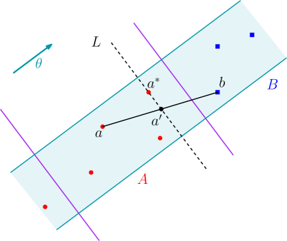
The construction relies on partitioning the plane into strips. Let be a unit vector. We define a strip in direction to be a region of the plane bounded by two lines, each parallel to . The width of the strip is the distance between its two bounding lines. We define the strip partition with direction and width (shorthanded as -strip partition) to be the unique partition of into strips of direction and width , where there is one strip that has a bounding line intersecting the point . Let ⊥ be a unit vector perpendicular to . A -strip partition with shift is obtained by shifting the boundary lines of the strip partition by .
Consider the following family of strip partitions: Let be the unit vector with angle , for . Let set i contains (1) the -strip partition with shift 0, and (2) the -strip partition with shift . Let . We call the strip partitions of the major strip partitions. Clearly, contains major strip partitions. We define to be a vector orthogonal to i; and we define ⊥ to be the set of all -strip partitions with shift 0, for every . We call the shift partitions of ⊥ the minor strip partitions. Every set i of major strip partitions is associated with a minor strip partition; notice that every major strip partition has an -factor smaller width to its orthogonal minor strip partition. See Figure 1.

Claim 2.9
For any two points such that and are -far, there exists some major strip partition such that (1) the points and are in the same strip of ; and (2) in the associated minor strip partition , the points and are in different strips.
-
Proof
Let denote the vector . There exists some such that the angle between the vector i and is at most . We write as a linear combination of i and a vector orthogonal to : . As the angle between and i is at most (and ), we have
Let i be the set of major strip partitions in direction i. As , and i consists of shifted strip partitions of width , there is some major strip partition in which and are in the same strip. Further, every strip in the associated minor strip partition has width , so the fact that implies that and are in different strips of . This proves the claim.
For every major strip partition in , we now construct a tree which preserves approximately distances between points that lie in the same major strip but different minor strips. The following is the key claim.
Claim 2.10
Let be a strip from a major strip partition in , with direction . Let and be two strips from a minor strip partition in , both with direction ⊥. Then there is a tree on such that for every and , In particular, if and are -far, then .
-
Proof
For any point , we define to be the inner product . Let and . As and belong to different minor strips in direction ⊥, without loss of generality for every and . Let . We claim that for any and ,
(1) To show this, consider the line segment between and . Let be the line in direction ⊥ that passes through . Because , line and segment intersect at some point in the slab ; see Figure 2. (Note that is not the projection of onto .) The distance can be no greater than the width of the slab, so . By triangle inequality, we have
Let be the star centered at , with an edge to every other point ; the weight of the edge between and is . For any and , we clearly have , and Equation (1) guarantees that .
We can now prove Lemma 2.8.
-
Proof
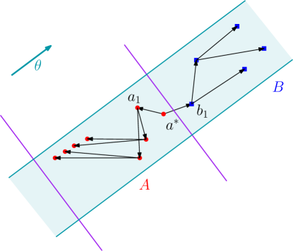
Let be the set of major strip partitions defined above. Let be an arbitrary major strip partition in , and let be the associated minor strip partition in ⊥. For each pair of strips and in , we define tree as follows: For every strip in , apply Claim 2.10 to construct a tree on (a subset of) that preserves distances between and ; and let be the tree obtained by joining together the trees from all strips in . To join the trees, we build a balanced binary tree from the roots of for all strips in . The tree cover consists of the set of all trees , for every major strip partition and every pair of strips in the associated minor strip partition .
To bound the size of , observe that (1) there are at most major strip partitions containing points in , and (2) for every strip in a major strip partition, at most strips in the associated minor strip partition contain points in (recall that point set has diameter ). Thus contains trees.
To bound the stretch, let and be arbitrary points in . By Claim 2.9, there exists some major strip partition such that (1) and are in the same strip in ; and (2) and are in different strips and of the associated minor strip partition . Thus Claim 2.10 implies that tree satisfies .
To bound the diameter, let be a major strip partition and let be a major strip in . Observe that is a star and the distance from the root of to any other point in is at most . The roots of trees corresponding to strips in are connected by a binary tree by construction. Each edge of this binary tree is of length at most . The number of strips in is upper bounded by . Hence, the height of the binary tree is at most . This means that the diameter of the resulting tree is at most .
Running Time.
The inner product between each point with each vector i can be precomputed using operations. For a major strip , finding the maximum point in the intersection between and each of its minor strip only need time proportional to the number of points in . Those points are chosen as roots of the stars corresponding to . For each root, constructing the corresponding star requires time. There are roots for each major strip. Hence, the total time complexity of constructing the -partitial tree cover is:
Therefore, the time complexity of constructing the tree cover is .
2.3 Partial tree cover with Steiner points
This part is devoted to the proof of Theorem 1.2 for ; the argument for dimension is deferred to Section 3.2.
Lemma 2.11
Let be a set of points in with diameter . For every constant , there is a Steiner -partial tree cover with stretch for with trees, where each tree has diameter at most .
Consider a square of side-length containing , and let be an arbitrary constant. Divide the square into vertical slabs of width and height , and into horizontal slabs of width and height .
Observation 2.12
For any two points such that and are -far, there exists either a horizontal or a vertical slab such that and are from different sides of the slab.
-
Proof
Suppose towards contradiction there are two adjacent horizontal slabs containing both and and also two adjacent vertical slabs containing both and . The distance between and is at most , contradicting the assumption that and are -far.
For each horizontal (resp. vertical) slab , we consider the horizontal (resp. vertical) line segment that cuts the slab into two equal-area parts. The length of is . Let be an integer. We partition into intervals, called , each of length . For each point , we construct tree by adding edges between and every point in . Finally, connect the points using a straight line and let be the resulting tree. The diameter of this tree is at most .
Claim 2.13
For any two points such that and are -far, there exists a slab and an integer such that .
-
Proof
By Observation 2.12, there exists a slab such that and are in different sides of it. Without loss of generality assume that is horizontal. By construction, we partition the middle interval of into intervals each of length . Let be the intersection between and , and let be the closest point to . Let be the projection of to . Hence, . Using the triangle inequality, we have:
(2) Observe that . Thus, . Similarly, . Combining with Equation 2, we get:
We now prove Lemma 2.11. Let be the set containing trees for every horizontal or vertical slabs and every index . There are horizontal and vertical slabs, so contains trees. It follows immediately from 2.13 that is a Steiner -partial tree cover for with stretch .
Running Time.
For a set , creating the set of slabs can be done in time. For each slab, finding a net of the middle line takes time. For each Steiner point, it requires time to create a tree connecting that point to everyone in . Totally, the time complexity is . Therefore, the time complexity of constructing the tree cover is .
3 Tree Cover in Higher Dimensions
3.1 Non-Steiner tree covers
We now prove an analog of Lemma 2.8 in , for any constant . The definition of strip partition and the sets and ⊥, are different in than in . Let be a vector. An -strip with direction and width is a convex region such that there is a line in such that every point in the strip is within distance at most of . The line is called the spine of the strip. An -strip partition is a partition of into -strips. For the construction of the major strip partitions , we use the following well-known lemma, slightly adapted from a version in the textbook by Narasimhan and Smid [NS07].
Lemma 3.1 (Cf. Lemma 5.2.3 of [NS07])
Let be a number in . There is a set of vectors in such that (1) contains vectors, and (2) for any vector in , there is some vector such that the angle between and is at most .
We also use a variant of the shifted quadtree construction of Chan [Cha98] (which follows immediately from our Lemma 2.1).
Lemma 3.2 (Cf. [Cha98])
For any constant , there is a set of partitions of into hypercubes of side length such that (1) there are partitions in , and (2) for every pair of points with , there is some partition where and are in the same hypercube in .
Let be a vector in . We define to be the hyperplane orthogonal to . We can view as a copy of . Let be an arbitrary partition of into -hypercubes with side length . This partition induces an -strip partition with direction and width : for every hypercube in the partition , the corresponding strip is defined by . We denote this strip partition as . The fact that has width follows from the fact that every point in a -hypercube of side length is within distance of the center point of the hypercube.
We now define the set of major strip partitions. Let be the set of vectors provided by Lemma 3.1, setting the parameter . For every , let denote the set of partitions of into -hypercubes of side length , as guaranteed by Lemma 3.2. The set contains the -strip partitions associated with every . Define . The following observation is immediate from Lemma 3.2:
Observation 3.3
Let be a vector in . If and are two points whose projections onto are within distance , then there is some strip partition in with a strip containing both and .
We now define ⊥, the set of minor strip partitions. For every , let ⊥ be some arbitrary vector that is orthogonal to . Let be an arbitrary partition of into -hypercubes with side length . Define ⊥ to be the set containing the -strip partition for every . With these modified definition of and ⊥, the claims from the case generalize naturally.
-
\the@itemx
The proof of Claim 2.9 is similar to the case. We break into a component parallel to and a component that lies in the hyperplane orthogonal to ; the former has length and the latter has length . Observation 3.3 (together with the upper-bound on ) guarantees that there is some major strip partition in direction in which and are in the same strip. The lower bound on implies that and are in different strips of the associated minor strip partition in direction ⊥.
-
\the@itemx
In the proof of Claim 2.10, the only difference is that the line in the 2D case is replaced by a hyperplane orthogonal to . To show that , we argue as follows. Hyperplane intersects the spine of the strip at some point ; as the width of the strip is , every point in that is in the strip (which includes and ) is within distance of . Triangle inequality proves the claim, and the rest of the proof carries over.
-
\the@itemx
The proof of Lemma 2.8 carries over almost exactly. The size of is . For every major strip partition , there are pairs of strips in the corresponding minor strip partition of ⊥, and thus the tree cover contains trees. The stretch bound carries over without modification.
-
\the@itemx
The diameter of each of the trees is . Every major strip partition is induced by set of -hypercubes with side length . Since the diameter of the point set is , the number of hypercubes required is at most . The same argument as in the 2-dimensional case implies the claimed bound on the diameter. The height of the binary tree is at most and each edge is of length at most . The diameter is at most .
Together with the reduction to a fixed scale (Lemma 2.4), this proves Theorem 1.1.
Running Time: The running time analysis is similar to the case. The inner product between each point to each direction vector can be precomputed in time. For each major strip , there are at most pair of minor strips that intersect . Hence, the total running time to construct a -partial tree cover is:
Then, the time complexity of constructing the tree cover is .
3.2 Tree covers with Steiner points
The construction for -dimensional Euclidean space is a direct generalization of two-dimensional case. Consider a hypercube of side length . We divide the hypercube by each coordinate into slabs of height ; all other sides have length . One can think of each slab as a -dimensional rectangle, joined by two -hypercubes that are distance away from each other. Analog of Obs. 2.12 follows.
Observation 3.4
For any two points such that and are -far, there exists a slab such that and are from different sides of it.
Each tree is constructed similarly to the two-dimensional case. For each slab, we find a -net for the -hypercube at the middle of each slab. For each net point , we create a tree connecting to every vertex in . The proof follows similarly. The total number of trees is
The diameter can be bounded by , as in the 2-dimensional argument.
Running Time: Creating the set of slabs requires time equal to the number of slabs, which is . For each slab, we find a -net of a -hypecube, which has points. For each Steiner point, we connect it to every point in in time. Hence, the total time complexity is:
Then, the time complexity of constructing the tree cover is .
4 Constant degree constructions
In this section, we prove the following theorem.
Theorem 4.1
For every set of points in and any , there exists a tree cover with stretch and trees such that every metric point has a bounded degree.
Our tree cover construction is a collection of trees, each of which possibly uses a copy of the same point many times. Each tree is constructed iteratively, going from smaller scales to the larger ones. In Section 4.1 we use the degree reduction technique due to [CGMZ16] for each tree in the cover. This allows us to bound the degree in terms of the number of trees in the cover and the degree at a single scale in the construction. In Section 4.2, we show that the degree at a single scale is constant.
4.1 Bounding the degree of metric points
Consider a single tree in the cover. Our tree cover construction from Section 2.2 does not use Steiner points, but it still might consider the same point from the metric across multiple levels of construction. Even if at each level of the construction every node has a bounded degree (which we show how to achieve in Section 4.2) the degree of each metric point might still be unbounded. To remedy this, we apply the degree reduction technique of [CGMZ16].
Start from the tree cover construction from Section 2 and fix a tree from the cover. Let be the same as in Section 2.1. Without loss of generality, assume the tree was constructed in the congruence class . Assume that at the every level of the construction, the edges of the tree are oriented from the parents to the children so that the outdegree of each node is and indegree is . We show how to bound the degree of every point of the metric with respect to .
Let be the highest quadtree level at which point is considered as a representative. For every edge in , we orient it from to if . If , break the ties according to the tree structure, from children towards parent. We use to denote the set of arcs obtained in this way. Note that , since we do not change any edges. Next, we describe the modification of , where we replace some edges of and obtain the set of . Let be a vertex at level and let be the set of edges used in the tree constructed at level . Let be the set of endpoints of edges in oriented into . Let . Suppose that the indices in are ordered increasingly. Next we modify arcs going into as follows. Keep directed into . For we pick an arbitrary vertex and for each point replace arc by an arc .
Claim 4.2
If at every level has an outdegree , then every metric point has outdegree . Moreover, every node with an outgoing edge at level ceases to be considered at levels higher than .
-
Proof
Consider an arc , i.e., an edge directed from towards . This means that . Let be the level at which was added to . Recall that the edges are added while handling a single quadtree cell at level and only one point from the cell is chosen a representative for the subsequent handling of level . If , this means that is a representative and does not exist on any subsequent level starting from . If , then neither nor are representatives, since the representative exists at a level higher than . Hence, does not exist on any subsequent level starting from . In conclusion, can have outgoing edges only at a single level of construction.
Claim 4.3
If at every level has an outdegree and indegree , then every metric point has degree with respect to at most .
-
Proof
Consider a metric point . There are at most edges directed out of by Claim 4.2. Out of the edges that were directed into in , there are only edges from that remained directed into . There are at most such edges. Finally, some new edges might have been attached to due to the modification into . Consider an arc directed out of ; there is a unique level where is in . Only edges of the form at level can be redirected to by the modification process; each such must be an in-neighbor of at level . A counting argument shows that for each arc going out of , there are at most new arcs attached to , each attribute to an in-neighbor of in before the modification; and there are possible choices of , all being the out-neighbors of . Putting everything together, the bound on the degree is .
We next show that the modification of the edges of does not create cycles.
Claim 4.4
The modified tree does not contain cycles.
-
Proof
Suppose towards contradiction that the modified contains a cycle and let be the first edge in the modification process whose insertion caused a cycle. Recall that the arc gets inserted in place of arc , where and , for some levels and . Since introduces a cycle, this means that contains an alternative path between and . By Claim 4.2, node does not exist at level higher than . Hence, the path appears at some level lower than . In the original tree , there were edges and . Together with the path between and , this creates a cycle in the original , a contradiction.
Next, we show that the stretch does not increase by more than a factor.
Claim 4.5
Let be the metric induced by . Then, for every , it holds .
-
Proof
It suffices to show that for an arc that is removed from it holds . Let . By construction, since is removed, there exists points , such that , and for : , and . Recall that we use to denote the diameter of a quadtree at level .
Observation 4.6
For every , .
Applying 4.6 inductively, we can prove that for every . We can also bound . By triangle inequality can be upper bounded by the length of the path .
In the next subsection, we show that and . Plugging in Claim 4.3, we obtain the bound of on the degree of every node in the metric.
4.2 Bounding the degree of tree nodes
Recall our construction from Section 2.2. Consider a single strip and the sets and as in the proof of 2.10. Let be the direction of strip . The tree handling the distances between and is a star rooted at a point . We describe three different constructions. The first construction achieves a constant degree but it requires scaling after which the number of trees grow by a factor of roughly . The second construction achieves degree of roughly and does not require any scaling. The third construction achieves degree 5 and requires scaling so that the number of trees grows by a factor of roughly .
Constant degree, simple attempt.
Let be the set of points in , sorted in decreasing order with respect to . We make a balanced binary tree rooted at such that for every node and its parent , . To do so, we mark as visited and make it the root of . Next, we scan the points in order, make child of the node in that was visited earliest and still has 0 or 1 children, then mark visited. We similarly construct satisfying that for every node and its parent , . Finally, let be the tree rooted at having subtrees and as its children.
Recall that, during the reduction to a single scale (Lemma 2.4), we only construct the partial tree covers of Section 2.2 on representative points contained in a quadtree cell. Since is balanced, it has height . Similarly, the height of is . In other words, between any node in and any node in there exists a path in consisting of at most edges.
We next prove the bound on the stretch between two points and that are -far. The proof follows the lines of 2.10. Consider line and let be the points on the path from to in . For , let be the intersection of with a line101010In higher dimensions, we consider the hyperplane orthogonal to . orthogonal to that passes through ; as the width of the strip is no more than , we have . By construction, every path in between a point in and a point in goes up the subtree , passes through the root and goes down the tree . In other words, we have that for every it holds that and . In addition, . We have . Thus, the length of the path in is
| by triangle inequality | ||||
The above stretch argument guarantees that preserves path between any point in and any point in up to a factor of . Applying the same degree reduction step for every strip in the strip partition and for every strip partition in the family , we obtain a tree cover with trees and stretch . To complete the argument, we need to scale the parameters. Let , so that the tree cover has stretch . The number of trees expressed in terms of ′ is , for .
Degree .
Let be the set of points in , sorted in decreasing order with respect to . Recall that the direction of the major strip is and the direction of the minor strip is ⊥. We build a binary tree rooted at as follows. Let the interval corresponding to be . Recall that the width of the strip is . Let be the set of active intervals, consisting of two elements: , corresponding to the future left child of (if any) and corresponding to the future right child of (if any). The elements of form a partition of at all times. Scan the points in order and perform the following. Let be the currently scanned point and let be its distance from the left border of the strip. Go over all the intervals in and see which one contains . (Such an interval exists because forms a partition of .) Let be such an interval. Add at the corresponding place in the tree. Let . Create two new intervals: corresponding to the left child of and , corresponding to the right child of . Note that after this, still forms a partition of . This concludes the description of . The tree is constructed analogously. Finally, the tree is obtained by attaching the roots of and as the left and right child of .
We next analyze the stretch. Consider two points and that are -far. Let be the path from (which is the root of ) to in and let be the path from to in . For two points and , let and similarly . Let and . Using this notation, we observe that . The second observation is that . This is because form a geometrically decreasing sequence. Similarly, . Using these two observations, we can upper bound the distance between and in as follows.
The argument for higher dimensions carries over almost exactly. The intervals used in the argument become -hypercubes. Consider a tree node and an interval corresponding to it. We partition the interval into subintervals of twice the smaller side length. Those subintervals correspond to the children of . To argue the stretch, we split the distance between points and in into two components: one along the vector and the remaining orthogonal part that lies in . The component along is at most and the component in is at most , due to the geometrically decreasing interval sizes.
Finally, we bound the diameter of each of the trees. Using analysis similar to the one used for the stretch, we conclude that the diameter of a tree corresponding to a single strip is at most . The trees of different major strips in a major strip partition are connected via a binary tree. As in Section 3.1, the height of the binary tree is at most . Hence, the overall degree is . The diameter of the tree is at most .
Constant degree.
We next explain a tweak which leads to degree 5. Instead of constructing a -ary tree for each strip we can work with a binary tree. Tree is built as follows. Let be the interval corresponding to . We assign level to each node in the tree, ranging from to . The level of is 1. The future children of are at level . In general, the children of a node at level are at level and the children of a node at level are at level . The set of active intervals consists of , corresponding to the left child of and . Once again, we maintain the property that is a partition of . Scan the points in that order and le t be the currently scanned point and the -dimensional vector of distances from each of the sides of the strip. Find the interval in where belongs to and place at the corresponding place in the tree. Let be the level of . Let . Split into corresponding to the left child of and corresponding to the right child of . Replace with and in . This concludes the description of the binary tree.
The stretch argument remains almost the same, except that , which is times larger than before. The reason is that every hops down the tree, we incur an additive stretch of after which the additive stretch reduces by a factor of two. Using the same argument as before, we conclude that . By scaling the stretch, we get that the number of trees increases by a factor of .
5 Application to Routing
In this section, we show an application of our tree cover to compact routing scheme. First, we give some background on the problem. A compact routing scheme is a distributed algorithm for sending messages or packets of information between points in the network. Specifically, a packet has an origin and it is required to arrive at a destination. Every node in the network contains a routing table, which stores local routing-related information, and a unique label, sometimes also called address. In the beginning, the network is preprocessed and every node is assigned a routing table and a label. Given a destination node , routing algorithm is initiated at source and is given the label of . Based on the local routing table of and the label of , it has to decide on the next node to which the packet should be transmitted. More formally, the algorithm outputs the port number leading to its neighbor . Each packet has a message header attached to it, which contains the label of the destination node , but may also contain other helpful information. Upon receiving the packet the algorithm at node has at its disposal the local routing table of and the information stored in the header. This process continues until the packet arrives at its destination, which is node . The stretch of the routing scheme is the ratio between the distance packet traveled in the network and the distance in the original metric space.
We consider routing in metric spaces, where each among points in the metric corresponds to a network node. In the preprocessing stage, we choose a set of links that induces an overlay network over which the routing must be performed. The goal is to have an overlay network of small size, whilst also optimizing the tradeoff between the maximum storage per node (that is, the size of routing tables, labels, and headers) and the stretch. In addition, one may try to further optimize the time it takes for every node to determine (or output) the next port number along the path, henceforth decision time, and other quality measures, such as the maximum degree in the overlay network.
There are two different models, based on the way labels are chosen: labeled, where the designer is allowed to choose (typically ) labels, and name-independent, where an adversary chooses labels. Similarly, depending on who is choosing the port numbers, there is a designer-port model, where the designer can choose the port number, and the fixed-port model, where the port numbers are chosen by an adversary. Our routing scheme works in the labeled, fixed-port model. For an additional background on compact routing schemes, we refer the reader to [Pel00, TZ01b, FG01, AGGM06].
In this section, we prove Theorem 1.3.
5.1 Routing in trees
We first explain the interval routing scheme due to [SK85]. Let be a given routed tree. We first preprocess the tree by performing a DFS on it and marking for every node the timestamp at which it got visited, . For every node , let be the maximum among the children of . The label of node consists of and requires bits of storage. The routing table of node consists of the port number leading to its parent in (unless is a root), and for each child of , the port number leading to together with , . This requires bits. Specifically, it requires bits for trees of constant degree, which is the case for our construction. To route from some node to a destination , the routing algorithm has routing table of and the label of at its disposal. For every child of , if falls in the interval , . If such a exists, the algorithm outputs the corresponding port to and otherwise the algorithm outputs port to the parent of . Note that in bounded degree trees the aforementioned routing algorithm needs to inspect only a constant number of entries in order to decide on the next port.
5.2 Routing in Euclidean spaces
To route in a Euclidean space, first construct a non-Steiner tree cover with bounded degree, using Theorem 4.1. The routing table of each point consists of its routing table in each of the trees in the cover, which takes bits, since each tree is of a constant degree. The label for each point consists of its label in each of the trees in , which overall takes bits, together with an additional label of bits described in the next section (“identifying a distance-preserving tree”). Overall this label takes bits. To route from a point to some other point , the algorithm first identifies a tree in that preserves the distance up to a factor: this step is described in the next section. After that, the routing algorithm proceeds on the single tree as described before.
5.3 Identifying a distance-preserving tree
Given two points and in , we now describe how to identify a tree in that preserves the distance between and up to stretch. The total size of this label will be .
Review of tree cover construction.
We first recall the construction of Theorem 1.1. We have a collection of compressed quadtrees (for every and congruence classes (where ). For ease of notation, let denote the tree obtained by starting with and then contracting away all nodes except those at level for . We refer to as a contracted quadtree. Notice that if is a cell in the contracted quadtree with diameter , then the children of in have diameter . For every shift and congruence class , we construct a set of trees as follows: for every cell in , we arbitrarily choose a set of representative points, one from each child cell of in ; we construct a partial tree cover on the representative points; and we merge these partial tree covers together into a final set of trees. Our proof of correctness guarantees that, for any pair of points and , there is some contracted quadtree and some cell in with diameter , such that the two representative points and are -far. There is some tree in the partial tree cover of that preserves up to a factor , and this tree corresponds to the tree in the final tree cover of Theorem 1.1 that preserves up to a factor .
In Section 4.2, we constructed a tree cover in which each partial tree cover had bounded-degree. The construction is identical to that of Theorem 1.1, except that we use a slightly modified construction for the partial tree cover on the representative points (modified from Section 2.2).
In Section 4.1, we used the result of Section 4.2 to get a bounded-degree tree cover (proving Theorem 4.1). The trees constructed in this section are in one-to-one correspondence with the trees constructed in Section 4.2: if a tree in the cover of Section 4.2 preserves the distance between two points and up to a factor , the corresponding transformed tree from Section 4.2 will preserve the distance up to a factor .
For simplicity, we describe how to identify a distance-preserving tree in the tree cover of Section 4.2: for any and , we will find a tree such that . As described above, these trees are in one-to-one correspondence with the bounded-degree trees of Theorem 4.1 (which is the tree cover we actually use for routing).
Our labeling scheme will consist of a short label for each tree . For each , this label will let us identify a cell whose partial tree cover preserves the distance (if such a cell exists), as well as the index of the corresponding distance-preserving tree. To construct this label for , we will need the following simple observation:
Observation 5.1
Let and be points in , and let be a contracted quadtree. Suppose there is a cell of such that contains both and , and the representatives and are -far. Then, in the smallest-diameter cell that contains both and , the representatives and are -far. In other words, if we view and as leaves of , the lowest common ancestor of and guarantees that the representatives are -far.
5.3.1 Identifying a valid partial tree cover
In this subsection, we describe a labeling scheme that lets us identify a distance-preserving tree in a partial tree cover.
Lemma 5.2
Let be a point set with diameter . For any constant , there is a labeling scheme with -bit labels, such that given the labels of any two points , we can either certify that and are -far or that they are not -far.
-
Proof
Let be a point with coordinates . The label of consists of parts: for each coordinate , the label stores difference between and rounded to a multiple of ; that is, we store . Because the maximum such difference is (because the diameter of is ), the label takes bits in total.
Given the labels of any two points and , we can compute, for each coordinate, an estimate of their difference within accuracy . Thus, we can estimate distance between and within an accuracy of . If this estimated distance is at least , the , and so and are -far. Otherwise, if the estimated distance is smaller than , we have , and so and are not -far.
Notice that if a partial tree cover consists of trees, one tree in the cover can be identified with bits. We will allow these “IDs” of the trees to be fixed in advance.
Lemma 5.3
Let be a -partial tree cover for a point set , constructed as in Section 4.2, with . Let be a function that maps trees to unique identifiers. There is a labeling scheme for with -bit labels, such that given the labels of any two points , we can either return for some tree that preserves the distance up to a factor, or we can certify that and are not -far.
-
Proof
Recall from Sections 2.2 and 4.2 that the construction of the partial tree cover proceeds by constructing major strip partitions and minor strip partitions. The major strip partitions have width ; thus, in each major strip partition, there are strips that contain points in . The minor strip partitions have width ; thus, in each major strip partition, there are strips that contain points in . Every triple consisting of a major strip partition and two minor strips in the associated minor strip partition corresponds to some tree in the partial tree cover.
Label. For every point , the label consists of four parts:
-
\the@itemxvi
For each of the major strip partitions, store a -bit label identifying which strip in the major strip partition contains .
-
\the@itemxvi
Similarly, for each of the minor strip partitions, store a -bit label identifying which strip in the minor strip partition contains .
-
\the@itemxvi
Store the -bit label of Lemma 5.2.
-
\the@itemxvi
For each of the triples consisting of a major strip partition and two minor strips in the associated partition , store the -bit identifier (given by ) of the corresponding tree.
Size. The total size of all four parts is .
Label correctness. Suppose we have the labels of two points . First, we use the label of Lemma 5.2 to determine either (1) and are -far, or (2) and are not -far. In the latter case, we are done; we have a certificate that and are not -far.
In the former case, we use the labels to check if there is some major strip partition such that the points and are in the same strip of , and and are in different strips of the associated minor strip partition . If there is no such strip, then Claim 2.9 implies that and are not -far, and we are done. Suppose there is such a strip. By the construction in Section 4.2, this triple of major strip and minor strips corresponds to a tree in the partial tree cover . Claim 2.10 implies that . As and are -far, we have . Thus, we have identified a tree in that preserves the distance between and up to a factor.
-
\the@itemxvi
5.3.2 LCA Labeling Tools
Before constructing our distance label, we need a preliminary result on LCA labeling. For any two vertices and in a tree , let denote the lowest common ancestor of and . For any vertex in the tree, we say its weight is the number of descendants. We say a vertex is heavy if its weight is greater than half the weight of its parent, otherwise it is light. For any vertex , let denote the parents of light ancestors of . We remark on two important facts: (1) there are vertices cells in , and (2) the LCA of and is in . These facts are used in existing LCA labeling schemes. We will modify the labeling scheme of Alstrup, Halvorsen, and Larsen:
Lemma 5.4 (Corollary 4.17 of [AHL14])
Let be a tree, and let be a function that indicates some predefined -bit names for the vertices of . There is a labeling scheme on the vertices of that uses bits, such that given labels of any two vertices and , we can compute .
We will use a variant of their labeling scheme.
Lemma 5.5
Let be a tree. For every vertex , let be a function that indicates some predefined -bit names for the vertices of . There is a labeling scheme on the vertices of that uses bits, such that given labels of two leaves and , we can compute:
-
\the@itemxvi
, if
-
\the@itemxvi
, if
If , then we can compute both labels .
-
Proof
We first review the labeling scheme of [AHL14]. For every vertex , the label of consists of two parts. The first part (cf. [AHL14, Corollary 4.17]) is just a lookup table: for every vertex , we record the -bit name . The second part encodes information about the root-to-x path in the tree: in particular (cf. [AHL14, Lemma 4.13]), given labels for and , we can use the second part of the label to detect whether is in — and to look up in the lookup table, if is in fact in .
We are now ready to describe the label to identify a distance-preserving tree.
5.3.3 Labeling scheme
Let be the tree cover of Theorem 4.1, of size .
Label.
Let be a contracted quadtree used in the construction of . For each cell in , assign an arbitrary ordering to its children (so that we can specify a child of with bits.) Let be a vertex in , and treat as a leaf of . For every cell , we define to be a label consisting of three parts:
-
\the@itemxvii
(L1) Store bits to identify which child of is an ancestor of .
-
\the@itemxvii
(L2) Store bits to identify which child of is heavy (if there is a heavy child).
-
\the@itemxvii
(L3) Let be the representative point for . Let denote the partial tree cover at cell , and for each tree , define to be the -bit identifier of the tree of the final tree cover that contains . Store the label of from Lemma 5.3 (using ): with this label, for any two points we can either find a tree in that preserves the distances of the representative points up to a factor , or we certify that the representative points are not -far.
Lemma 5.5 gives us an LCA label for . For each contracted quadtree , store this label.
Size.
The label consists of bits. Thus, Lemma 5.5 gives us labels of size . There are quadtrees , so the label size is in total.
Decoding.
Suppose we have labels for and . For each , we use Lemma 5.5 to find information about . There are two cases:
-
\the@itemxvii
Case 1: is in . In this case, we have access to both and . We use the (L1) parts of labels and to identify the two children and of that contain and , respectively.
-
\the@itemxvii
Case 2: (Without loss of generality) is only in . Let denote the child of that is an ancestor of . Because is not the parent of a light ancestor of , we know that the child is heavy. Use the (L2) part of to identify the child . As before, use the (L1) part of label to identify the child that is an ancestor of .
Having identified and , we can now use the (L3) part of label to determine whether there is a tree that preserves the distance between the representatives of and up to a factor. If there is such a tree, return it; otherwise, check the next .
By the proof of correctness of Theorem 1.1, there is some contracted quadtree with a cell in which the representatives of and are -far; further, our Observation 5.1 guarantees that it suffices to check only the LCA of and in each contracted quadtree. Thus, this process (iterating over all contracted quadtrees, and checking the LCA of each) will eventually find a quadtree cell in which the representatives are -far, and thus (by Lemma 5.3), the (L3) part of the label will return a tree that preserves the distance of the representative points. By the proof of Claim 2.7, this tree preserves the distance between and up to a factor.
Acknowledgement.
Hung Le and Cuong Than are supported by the NSF CAREER Award No. CCF-2237288 and an NSF Grant No. CCF-2121952. Shay Solomon is funded by the European Union (ERC, DynOpt, 101043159). Views and opinions expressed are however those of the author(s) only and do not necessarily reflect those of the European Union or the European Research Council. Neither the European Union nor the granting authority can be held responsible for them. Shay Solomon is also supported by the Israel Science Foundation(ISF) grant No.1991/1. Shay Solomon and Lazar Milenković are supported by a grant from the United States-Israel Binational Science Foundation (BSF), Jerusalem, Israel, and the United States National Science Foundation(NSF).
References
- [ABN11] Ittai Abraham, Yair Bartal, and Ofer Neiman. Advances in metric embedding theory. Advances in Mathematics, 228(6):3026–3126, 2011.
- [ACRX22] Pankaj K Agarwal, Hsien-Chih Chang, Sharath Raghvendra, and Allen Xiao. Deterministic, near-linear -approximation algorithm for geometric bipartite matching. In Proceedings of the 54th Annual ACM SIGACT Symposium on Theory of Computing, pages 1052–1065, 2022.
- [ADD+93] Ingo Althöfer, Gautam Das, David Dobkin, Deborah Joseph, and José Soares. On sparse spanners of weighted graphs. Discrete & Computational Geometry, 9(1):81–100, 1993.
- [ADM+95] Sunil Arya, Gautam Das, David M Mount, Jeffrey S Salowe, and Michiel Smid. Euclidean spanners: short, thin, and lanky. In Proceedings of the twenty-seventh annual ACM symposium on Theory of computing, pages 489–498, 1995.
- [AG06] I. Abraham and C. Gavoille. Object location using path separators. In Proceedings of the Twenty-fifth Annual ACM Symposium on Principles of Distributed Computing, PODC ’06, pages 188–197, 2006. Full version: https://www.cse.huji.ac.il/~ittaia/papers/AG-TR.pdf. doi:10.1145/1146381.1146411.
- [AGGM06] Ittai Abraham, Cyril Gavoille, Andrew V. Goldberg, and Dahlia Malkhi. Routing in networks with low doubling dimension. In Proc. of 26th ICDCS, page 75, 2006.
- [AHL14] Stephen Alstrup, Esben Bistrup Halvorsen, and Kasper Green Larsen. Near-optimal labeling schemes for nearest common ancestors. In Proceedings of the Twenty-Fifth Annual ACM-SIAM Symposium on Discrete Algorithms, pages 972–982. SIAM, 2014.
- [AKP94] Baruch Awerbuch, Shay Kutten, and David Peleg. On buffer-economical store-and-forward deadlock prevention. IEEE transactions on communications, 42(11):2934–2937, 1994.
- [AKPW95] Noga Alon, Richard M. Karp, David Peleg, and Douglas West. A graph-theoretic game and its application to the -server problem. SIAM Journal on Computing, 24(1):78–100, 1995. doi:10.1137/s0097539792224474.
- [AP92] Baruch Awerbuch and David Peleg. Routing with polynomial communication-space trade-off. SIAM J. Discret. Math., 5(2):151–162, may 1992. doi:10.1137/0405013.
- [AZ23] Alexandr Andoni and Hengjie Zhang. Sub-quadratic (1+eps)-approximate euclidean spanners, with applications. 2023.
- [BFN22] Yair Bartal, Ora Nova Fandina, and Ofer Neiman. Covering metric spaces by few trees. Journal of Computer and System Sciences, 130:26–42, 2022.
- [BT22] Sujoy Bhore and Csaba D Tóth. Euclidean steiner spanners: Light and sparse. SIAM Journal on Discrete Mathematics, 36(3):2411–2444, 2022.
- [CCG+98] M. Charikar, C. Chekuri, A. Goel, S. Guha, and S. Plotkin. Approximating a finite metric by a small number of tree metrics. In Proceedings 39th Annual Symposium on Foundations of Computer Science (Cat. No. 98CB36280), pages 379–388. IEEE, 1998.
- [CCL+23a] Hsien-Chih Chang, Jonathan Conroy, Hung Le, Lazar Milenkovic, and Shay Solomon. Covering planar metrics (and beyond): O(1) trees suffice, 2023. Accepted to FOCS 2023.
- [CCL+23b] Hsien-Chih Chang, Jonathan Conroy, Hung Le, Lazar Milenkovic, Shay Solomon, and Cuong Than. Shortcut partitions in minor-free graphs: Steiner point removal, distance oracles, tree covers, and more, 2023. Accepted to SODA 2024.
- [CGMZ16] T.-H. Hubert Chan, Anupam Gupta, Bruce M. Maggs, and Shuheng Zhou. On hierarchical routing in doubling metrics. ACM Transactions on Algorithms (TALG), 12(4):1–22, 2016.
- [Cha98] Timothy M. Chan. Approximate nearest neighbor queries revisited. Discret. Comput. Geom., 20(3):359–373, 1998.
- [DYL06] Feodor F Dragan, Chenyu Yan, and Irina Lomonosov. Collective tree spanners of graphs. SIAM Journal on Discrete Mathematics, 20(1):240–260, 2006.
- [EVDHM22] Jeff Erickson, Ivor Van Der Hoog, and Tillmann Miltzow. Smoothing the gap between np and er. SIAM Journal on Computing, (0):FOCS20–102, 2022.
- [FG01] Pierre Fraigniaud and Cyril Gavoille. Routing in trees. In ICALP, volume 2076 of Lecture Notes in Computer Science, pages 757–772. Springer, 2001.
- [FGNW17] Ofer Freedman, Paweł Gawrychowski, Patrick K. Nicholson, and Oren Weimann. Optimal distance labeling schemes for trees. In Proceedings of the ACM Symposium on Principles of Distributed Computing, 2017. doi:10.1145/3087801.3087804.
- [FVW93] Steven Fortune and Christopher J. Van Wyk. Efficient exact arithmetic for computational geometry. In Proceedings of the Ninth Annual Symposium on Computational Geometry, SCG ’93, page 163–172, New York, NY, USA, 1993. Association for Computing Machinery. doi:10.1145/160985.161015.
- [GH23] Zhimeng Gao and Sariel Har-Peled. Almost optimal locality sensitive orderings in Euclidean space. CoRR, abs/2310.12792, 2023.
- [GKL03] Anupam Gupta, Robert Krauthgamer, and James R. Lee. Bounded geometries, fractals, and low-distortion embeddings. In FOCS, pages 534–543. IEEE Computer Society, 2003.
- [GKR01] A. Gupta, A. Kumar, and R. Rastogi. Traveling with a Pez dispenser (or, routing issues in MPLS). In Proceedings 42nd IEEE Symposium on Foundations of Computer Science,FOCS’ 01, 2001. doi:10.1109/sfcs.2001.959889.
- [GPPR04] Cyril Gavoille, David Peleg, Stéphane Pérennes, and Ran Raz. Distance labeling in graphs. Journal of Algorithms, 53(1):85–112, 2004. doi:10.1016/j.jalgor.2004.05.002.
- [GR08] L. Gottlieb and L. Roditty. Improved algorithms for fully dynamic geometric spanners and geometric routing. In Proceedings of the 19th Annual ACM-SIAM Symposium on Discrete Algorithms, SODA’08, pages 591–600, 2008. doi:10.5555/1347082.1347148.
- [KLMN05] Robert Krauthgamer, James R. Lee, Manor Mendel, and Assaf Naor. Measured descent: a new embedding method for finite metrics. Geometric and Functional Analysis, 15(4):839–858, 2005. URL: http://dx.doi.org/10.1007/s00039-005-0527-6, doi:10.1007/s00039-005-0527-6.
- [KLMS22] Omri Kahalon, Hung Le, Lazar Milenković, and Shay Solomon. Can’t see the forest for the trees: navigating metric spaces by bounded hop-diameter spanners. In Proceedings of the 2022 ACM Symposium on Principles of Distributed Computing, pages 151–162, 2022.
- [LPY05] Chen Li, Sylvain Pion, and Chee-Keng Yap. Recent progress in exact geometric computation. The Journal of Logic and Algebraic Programming, 64(1):85–111, 2005.
- [LS22] Hung Le and Shay Solomon. Truly optimal Euclidean spanners. SIAM Journal on Computing, (0):FOCS19–135, 2022.
- [Mar88] Grigorii Aleksandrovich Margulis. Explicit group-theoretical constructions of combinatorial schemes and their application to the design of expanders and concentrators. Problemy Peredachi informatsii, 24(1):51–60, 1988.
- [MN06] Manor Mendel and Assaf Naor. Ramsey partitions and proximity data structures. In 2006 47th Annual IEEE Symposium on Foundations of Computer Science (FOCS’ 06), 2006. doi:10.1109/focs.2006.65.
- [NS07] Giri Narasimhan and Michiel Smid. Geometric spanner networks. Cambridge University Press, 2007.
- [Pel00] David Peleg. Proximity-preserving labeling schemes. J. Graph Theory, 33(3):167–176, mar 2000. URL: https://dl.acm.org/doi/10.5555/1379811.1379818, doi:10.5555/1379811.1379818.
- [SK85] Nicola Santoro and Ramez Khatib. Labelling and implicit routing in networks. Comput. J., 28(1):5–8, 1985.
- [Smi12] Michiel Smid. Notes on binary dumbbell trees. Unpublished notes, 2012. URL: https://people.scs.carleton.ca/~michiel/dumbbelltrees.pdf.
- [SSG89] David Salesin, Jorge Stolfi, and Leonidas Guibas. Epsilon geometry: building robust algorithms from imprecise computations. In Proceedings of the fifth annual symposium on Computational geometry, pages 208–217, 1989.
- [TZ01a] Mikkel Thorup and Uri Zwick. Compact routing schemes. In Proceedings of the thirteenth annual ACM symposium on Parallel algorithms and architectures, pages 1–10, 2001.
- [TZ01b] Mikkel Thorup and Uri Zwick. Compact routing schemes. In SPAA, pages 1–10. ACM, 2001.
- [TZ05] Mikkel Thorup and Uri Zwick. Approximate distance oracles. Journal of the ACM (JACM), 52(1):1–24, 2005.