Masked Autoencoders are PDE Learners

Abstract

Neural solvers for partial differential equations (PDEs) have great potential, yet their practicality is currently limited by their generalizability. PDEs evolve over broad scales and exhibit diverse behaviors; predicting these phenomena will require learning representations across a wide variety of inputs, which may encompass different coefficients, geometries, or equations. As a step towards generalizable PDE modeling, we adapt masked pretraining for PDEs. Through self-supervised learning across PDEs, masked autoencoders can learn useful latent representations for downstream tasks. In particular, masked pretraining can improve coefficient regression and timestepping performance of neural solvers on unseen equations. We hope that masked pretraining can emerge as a unifying method across large, unlabeled, and heterogeneous datasets to learn latent physics at scale.

1 Introduction

The physical world is incredibly complex; physical phenomena can be extremely diverse and span wide spatiotemporal scales—from neuron excitations to turbulent flow to even global climate. Importantly, many of these phenomena can be mathematically modeled with time-dependent partial differential equations. These PDEs are generally analytically intractable and require the use of numerical solvers to obtain approximate solutions. For complex phenomena, these solutions can often be slow to obtain; furthermore, different phenomena often require a careful design of tailored solvers.

Advances in deep learning in the past decade have led to the design of a novel class of solvers for PDEs. These neural solvers can be extremely fast and display resolution invariance; however, neural networks introduce training difficulties and a lack of error bounds. Many important advances have been made to address these challenges, with SOTA models achieving high accuracy on well-studied PDEs under certain configurations (Raissi et al. (2019),Lu et al. (2019), Li et al. (2020), Cao (2021), Brandstetter et al. (2022a), Li et al. (2023a)).

A current frontier in neural PDE solvers lies in generalizing solvers to different parameters, conditions, or equations, thereby avoiding the need to collect new data and retrain networks when given unseen PDE dynamics. Preliminary work in this space has explored many methods to achieve this, from directly conditioning on PDE coefficients (Takamoto et al. (2023), Lorsung et al. (2024), Shen et al. (2024)) to pretraining foundation models across various equations (Subramanian et al. (2023), McCabe et al. (2023), Hao et al. (2024)). Despite these advances, generalizable neural solvers remain a significant challenge. PDEs can be incredibly diverse and chaotic, and neural network predictions need to be not only semantically reasonable, but also numerically accurate.

As a step towards addressing these challenges, we propose adapting masked pretraining methods to PDEs. Specifically, we demonstrate that masked PDE modeling can learn latent representations to improve performance on downstream tasks even on unseen coefficients and PDEs. These results align with current research on PDE pretraining, however, we demonstrate learning on a self-supervised task—granting flexibility in selecting downstream tasks or equations to fine-tune on and the ability to pretrain on unlabeled, incomplete, or heterogeneous datasets. Additionally, our approach is agnostic to downstream architecture choices, allowing standard neural solvers to quickly finetune to new equations through conditioning on a pretrained model.

2 Related Work

2.1 Neural PDE Solvers

The field of neural PDE solvers has grown rapidly and has shown great advances in both the accuracy of solutions and the ability to adapt to different equations and boundary conditions. Infinite-dimensional neural operators (Li et al. (2020); Kovachki et al. (2023); Lu et al. (2019)) have shown impressive accuracy in solving time-dependent PDEs by learning the mappings between initial conditions and solutions. However, these methods alone have shown brittleness with respect to changing PDE coefficients or boundary conditions (Gupta and Brandstetter (2022); Lu et al. (2021)), prompting recent work to allow neural solvers to adapt to changes in PDE conditions.

A variety of approaches have considered adding PDE dynamics information to neural solvers. (Gupta and Brandstetter (2022)) benchmark different PDE conditioning methods across common architectures, while (Brandstetter et al. (2022a)) design message-passing neural solvers that benefit from PDE coefficient and boundary condition information. Beyond directly conditioning on PDE dynamics, a class of neural PDE solvers has proposed the addition of an encoder or adaptive network to inform a forecaster network of different PDE coefficients (Wang et al. (2021), Kirchmeyer et al. , Takamoto et al. (2023), Lorsung et al. (2024)). At an even broader level, (Yin et al. (2021)) and (Zhang et al. (2023a)) propose modifications to the PDE forecasting loss function to maximize shared learning across diverse PDE examples to meta-learn dynamics across parameters.

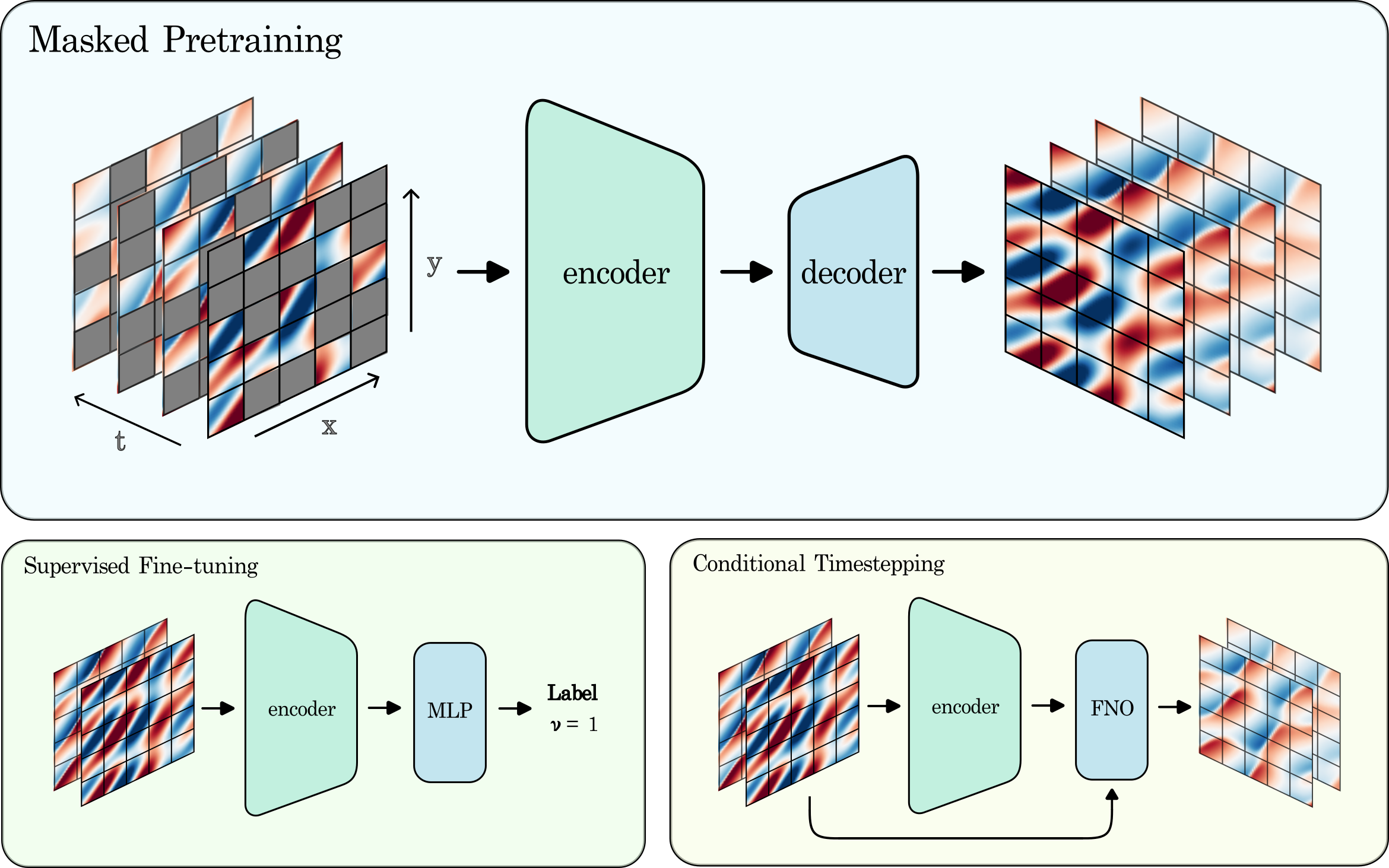
Figure 1: Masked Autoencoders are PDE Learners. We investigate the ability of autoencoders to learn diverse PDE dynamics through masked reconstruction. (Top) We pretrain an encoder on unmasked patches of spatiotemporal PDE data, while a decoder reconstructs the true data from latent embeddings and learned mask patches. (Left) We evaluate the encoder’s latent representation through regressing PDE coefficients on both interpolated and unseen equations. (Right) We show improved PDE timestepping performance through conditioning neural solvers on encoded PDE inputs.

2.2 Pretraining for PDEs

As an effort to work towards more generalizable PDE neural solvers, recent work has followed the success of pretraining and foundational models in the broader deep learning community. Based on contrastive pretraining methods in computer vision problems, (Chen et al. (2020), Schroff et al. (2015), Zbontar et al. (2021), Bardes et al. (2022)), contrastive PDE methods aim to leverage equation coefficients (Lorsung and Farimani (2024)), physical invariances (Zhang et al. (2023b)), or Lie point symmetries (Mialon et al. (2023) Brandstetter et al. (2022b)) to define similar or different PDE dynamics that can be organized in a latent space. Another approach in PDE pretraining follows observed in-context learning and emergent behavior in LLMs (Wei et al. (2022), Brown et al. (2020), Radford et al. ) to design neural PDE solvers that are capable of following prompted PDE examples to forecast unseen dynamics (Yang et al. (2023a), Chen et al. (2024)).

A more straightforward pretraining method focuses on directly training neural solvers to transfer to new PDE dynamics (Goswami et al. (2022), Chakraborty et al. (2022), Wang et al. (2022)). This approach has also been scaled by training neural solvers with large and diverse training sets to characterize its transfer behavior (Subramanian et al. (2023)). As a step toward foundational modeling, more principled training approaches have been proposed to learn PDE dynamics across diverse physics at scale. (Tripura and Chakraborty (2023)) design a combinatorial neural operator that learns different dynamics as separate modules, (McCabe et al. (2023)) use a shared embedding to auto-regressively learn multiple physics with axial attention, (Hao et al. (2024)) incorporate denoising with a scalable transformer architecture to show fine-tuning performance across diverse PDE datasets, and (Shen et al. (2024)) incorporate a unified PDE embedding to align LLMs across PDE families.

2.3 Masked Pretraining

Masked reconstruction is a popular technique popularized by the language processing (Devlin et al. (2018)) and vision (Dosovitskiy et al. (2020), Xie et al. (2021), He et al. (2021)) domains to pretrain models for downstream tasks. Masked modeling is a broad field that spans many masking strategies, architectures, and applications (Li et al. (2024)); this ubiquity is attributed to the ability of masked pretraining to increase performance in downstream tasks, suggesting that these models can learn meaningful context through masked reconstruction (Cao et al. (2022)). In the field of neural PDE solvers, masked pretraining has been initially explored to investigate its fine-tuning performance and data efficiency when applied to equations in the same family (Chen et al. (2024)). However, masked modeling still remains to be investigated when pretraining on datasets across equations, geometries, or resolutions; furthermore, it’s downstream performance to novel tasks or equations has not been characterized, which we believe may hold great potential.

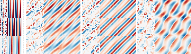
Figure 2: Masked PDE Modeling. In each triplet, the masked PDE data (left), autoencoder reconstruction (middle), and true PDE data (right) is shown. Additionally, we use a masking ratio of 60% in all examples. (Left) Masked reconstruction of unseen samples of the 1D KdV-Burgers equation, which interpolates between the Heat, Burgers, and KdV equations. (Right) Masked reconstruction of the 2D Heat, Advection, and Burgers equations displayed at selected timesteps. Note that a single autoencoder is used across all 2D samples.

3 Methods

In this section, we describe our methodology to train masked autoencoders for downstream PDE tasks, as shown in Figure 1. For 1D and 2D PDEs, we adopt ViT (Dosovitskiy et al. (2020)) and ViT3D (Arnab et al. ) architectures to act as an encoder and decoder for masked reconstruction according to (He et al. (2021)). Additionally, we study the addition of Lie augmentations (Brandstetter et al. (2022b)) to masked pretraining data, an approach that follows the use of data augmentations for vision or video pretraining (He et al. (2021); Xie et al. (2021); Feichtenhofer et al. ).

3.1 Masked Pretraining for PDEs

We employ a common approach of partitioning data into non-overlapping patches. A random subset of these patches is sampled to be masked and omitted from the encoder input. The encoder then embeds only the visible, unmasked patches through a series of Transformer blocks. At large masking ratios, this reduces the input complexity and allows for both larger encoders and lower computational complexity (He et al. (2021)).

The embedded patches are then recombined with mask tokens according to their position in the PDE trajectory. Positional embeddings are added again to preserve positional information before being decoded. An asymmetric design is used to further reduce training costs, as the decoder can be shallower and narrower because it is discarded in downstream tasks (He et al. (2021)). The decoded tokens are projected into the PDE space through a linear layer before reconstructing the output from the patches. Lastly, the output is compared to ground truth PDE data through an L1 loss.

3.2 Lie Point Symmetry Data Augmentations

To emulate a larger pretraining dataset, we consider augmenting the pretraining dataset with Lie point symmetries (Brandstetter et al. (2022b)). Given a PDE, one can derive or look up its symmetries as a set of transformations $\{g_{1},\dots,g_{i}\}$, each with a variable $\epsilon_{i}$ that modulates the magnitude of the transformation. At training time, we apply $g_{i}$ sequentially, each with a randomly sampled $\epsilon_{i}$ to augment PDE samples with a certain probability. This augmented PDE sample could represent a solution that has been shifted in space, time, or magnitude, among other transformations, but still propagates dynamics according to the original PDE. For a more detailed discussion of Lie point symmetries for PDEs, we refer the reader to (Olver (1986)) and (Mialon et al. (2023)).

4 Experiments

We test the fine-tuning performance of masked autoencoders on PDE regression and timestepping tasks in 1D and 2D. This approach is similar to vision or language domains; for example, pretraining on masked image reconstruction and fine-tuning to image classification or semantic segmentation ( He et al. (2021); Xie et al. (2021)). We find comparable performance gains: pretrained autoencoders are able to extract context from PDE trajectories to inform downstream tasks and provide higher performance across different equations and applications.

4.1 Equations Considered

Add information about time and spatial resolution.

1. 1D KdV-Burgers Equation We pretrain and evaluate downstream performance on a family of PDEs governed by the combined KdV-Burgers equation (Brandstetter et al. (2022a)).

   $$\partial_{t}u+\alpha u\partial_{x}u-\beta\partial_{xx}u+\gamma\partial_{xxx}u=\delta(t,x)$$ (1)

   This equation contains the heat, Burgers, KdV equations as corner cases. Furthermore, periodic boundary conditions are used with a forcing function and initial condition defined by $\delta(x,t)$.

   $$\delta(t,x)=\sum_{j=1}^{J}A_{j}sin(\omega_{j}t+2\pi l_{j}x/L+\phi_{j})$$ (2)

   $$u(0,x)=\delta(0,x)$$ (3)

   This setup follows (Bar-Sinai et al. (2019)) and (Brandstetter et al. (2022a)) to introduce randomness and periodicity into PDE solutions. This is implemented by sampling equation coefficients uniformly in $\alpha\in[0,1],\beta\in[0,0.5],\gamma\in[0,6]$, and sampling forcing coefficients uniformly in $A_{j}\in[-0.5,0.5],\omega_{j}\in[-0.4,0.4],l_{j}\in{1,2,3},\phi_{j}\in[0,2\pi)$ while setting $J=5,L=16$. We generate samples with resolution $(n_{t},n_{x})=(250,100)$.

2. 1D Advection and KS Equations: The linear advection (4) and Kuramoto-Sivashinsky (5) equations are considered to evaluate fine-tuning to unseen equations.

   $$\partial_{t}u+c\partial_{x}u=0,\quad c\in[0.1,2.5]$$ (4)

   $$\partial_{t}u+u\partial_{x}u+\partial_{xx}u+\partial_{xxxx}u=0$$ (5)

   In both equations, initial conditions are randomly sampled according to equation (2) and periodic boundary conditions are enforced. We generate advection samples with resolution $(n_{t},n_{x})=(250,100)$ and KS samples with resolution $(n_{t},n_{x})=(150,100)$.

3. 2D Heat, Advection and Burgers Equations: We pretrain and evaluate downstream performance on a combined set of 2D Heat (6), Advection (7), and Burgers (8, 9) equations under periodic boundary conditions.

   $$\partial_{t}u+\nu(\partial_{xx}u+\partial_{yy}u)=0$$ (6)

   $$\partial_{t}u+c_{x}\partial_{x}u+c_{y}\partial_{y}u=0$$ (7)

   $$\partial_{t}u+\alpha_{x}u\partial_{x}u+\alpha_{y}v\partial_{y}u-\beta(\partial_{xx}u+\partial_{yy}u)=0$$ (8)

   $$\partial_{t}v+\alpha_{x}u\partial_{x}v+\alpha_{y}v\partial_{y}v-\beta(\partial_{xx}v+\partial_{yy}v)=0$$ (9)

   We sample the coefficients of the equation uniformly in $c_{x}\in[0.1,2.5],c_{y}\in[0.1,2.5],\nu\in[3\mathrm{e}{-3},3\mathrm{e}{-2}],\alpha_{x}\in[0.5,1],\alpha_{y}\in[0.5,1],\beta\in[3\mathrm{e}{-3},2\mathrm{e}{-2}]$. Furthermore, we generate initial conditions through a similar approach using a truncated Fourier series in 2D:

   $$u(x,y,0)=\sum_{j=1}^{J}A_{j}sin(2\pi l_{xj}x/L+2\pi l_{yj}y/L+\phi_{j})$$ (10)

   Initial condition coefficients are sampled identically to 2, with $A_{j}\in[-0.5,0.5],\omega_{j}\in[-0.4,0.4],l_{xj},l_{yj}\in{1,2,3},\phi_{j}\in[0,2\pi)$ while setting $J=5,L=2$. Additionally, samples are generated with a resolution of $(n_{t},n_{x},n_{y})=(100,64,64)$.

4.2 PDE Coefficient Regression

We evaluate the latent space of masked autoencoders after pretraining on the KdV-Burgers equation in 1D and the combined Heat, Advection, and Burgers equations in 2D. This is done through regressing equation coefficients after discarding the decoder and training a linear model on top of the encoder’s class embedding. Specifically, we use a VIT model for 1D regression with 1.6M parameters and a VIT3D model for 2D regression with 3.5M parameters. We compare end-to-end finetuning with a supervised baseline trained with a randomly initialized encoder and a frozen encoder. This is similar to pretraining methods in vision—masked autoencoders are both linearly evaluated and fine-tuned end-to-end. Additionally, we fine-tune on regressing coefficients from unseen equations in 1D, and present the results in Table LABEL:tab:regression.

1D PDE Regression: We pretrain on a set of 4096 unlabeled KdV-Burgers equation samples and fine-tune on 4096 labeled KdV-Burgers samples and 2048 labeled Advection and KS samples. We consider three coefficients $[\alpha,\beta,\gamma]$ in the KdV-Burgers equation to regress from the test set. Furthermore, we regress the advection speed $c$ and a set of $2J$ initial condition coefficients $[A_{j},\omega_{j}]$ from the advection and KS test sets, respectively. In particular, for the 1D KS equation, we omit samples from the first 25 timesteps to mask the initial conditions.

2D PDE Regression: In two dimensions, we use a pretraining set of 3072 unlabeled Heat/Advection/Burgers equation samples and fine-tune on 3072 labeled Heat/Advection/Burgers equation samples. We consider six coefficients $[c_{x},c_{y},\beta,\nu,\alpha_{x},\alpha_{y}]$ to regress from the combined Heat, Advection, and Burgers test set.

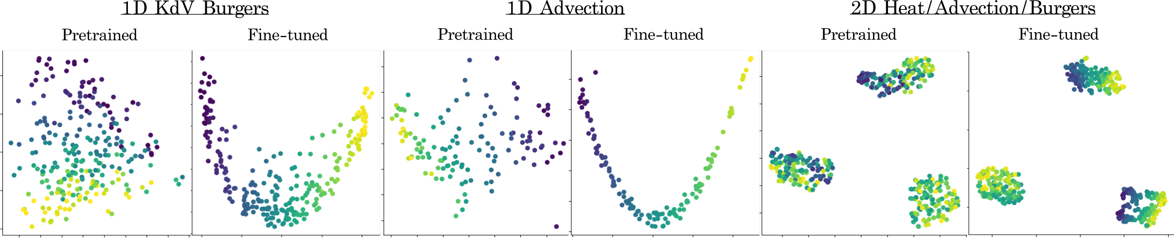
Figure 3: MAE Latent Space. We plot encoder class token embeddings after masked pretraining and after fine-tuning with coefficient labels. Note that the model does not see coefficient values during pretraining yet is still able to learn approximate trends in PDEs. (Left) Embeddings of 1D PDEs. We use a 2D PCA as dimensionality reduction and color embeddings by ascending $\alpha$ and $c$ coefficients of the KdV-Burgers and Advection equations, respectively. (Right) Embeddings of 2D PDEs. We use a 2D t-SNE as dimensionality reduction and color embeddings by ascending $\nu$, $c_{x}$, and $\alpha_{x}$ coefficients of the Heat, Advection, and Burgers equations.

Table 1: Coefficient Regression Task. Test MSE errors of different models across equations. Encoders are pretrained on equations in bold. Errors are averaged over three seeds in all experiments, and given multiplied by 1e-3.

	1D			2D
Model	KdV-Burgers	Adv	KS	Heat/Adv/Burgers
Supervised	11.92	0.772	104.36	1.203
Pretrained/Frozen	2.925	116.1	104.33	4.519
Pretrained/Fine-tuned	0.579	0.130	104.23	0.892

In general, we observe improved regression performance from the use of a pretrained initialization compared to random initialization when regressing coefficients. For the 1D KdV-Burgers equation, this is true even when the encoder is frozen; however, end-to-end fine-tuning is necessary for extrapolation to new equations and in 2D. We hypothesize that this could be due to the small size of the 2D pretraining data set, consisting only of 3072 samples. Furthermore, in the 1D KS equation, all models converge to the same performance when regressing the initial coefficients. We hypothesize that this is due to the equation’s chaotic behavior and relatively few training samples, since both the supervised and fine-tuned models tend to overfit to initial coefficients on the training set. This behavior could also suggest that masked autoencoders learn how PDEs evolve over different coefficients or equations, rather than how PDEs evolve over different initial conditions.

We visualize the latent space learned by masked autoencoders by plotting the encoder’s class embedding across different equations in Figure 3. Interestingly, the class embedding is able to approximately differentiate PDE dynamics even before seeing the labeled data. Additionally, the phenomenon is observed on unseen equations; 1D advection samples show trends in the latent space despite only pretraining on unlabeled KdV-Burgers samples. After fine-tuning, the latent space predictably organizes to separate samples originating from different coefficients well.

In two dimensions, the model is able to organize samples into Heat, Advection, and Burgers clusters in the latent space. Furthermore, within each cluster, the encoder is able to approximately differentiate equations by their coefficients. Again, the model is able to learn this latent representation before seeing labeled data; after fine-tuning, the data is similarly clustered but better organized by their coefficients.

4.3 PDE Timestepping

We consider the use of autoencoder embeddings to condition neural operators in PDE timestepping. To investigate the effect of autoencoder conditioning, we train three model variants: Fourier Neural Operator (FNO) (Li et al. (2020)), FNO conditioned on a pretrained but frozen encoder, and FNO conditioned on a pretrained and end-to-end finetuned encoder. For 1D PDEs, we use VIT (1.6M) and FNO1D (0.8M) models; for 2D PDEs we use VIT3D (3.5M) and FNO2D (2.7M) models.

To condition neural operator models, we employ a strategy introduced in (Gupta and Brandstetter (2022)), whereby we project embeddings into the Fourier domain and multiply embeddings with FNO spectral weights. Additionally, the embeddings are linearly projected and added to the residual connection and the Fourier branch. Furthermore, to improve temporal stability, we implement the temporal bundling and pushforward trick from (Brandstetter et al. (2022a)). At test time, we provide an initial window of PDE data and autoregressively rollout future timesteps; accumulated error between autoregressive predictions and ground truth data is averaged and presented in Table LABEL:tab:timestepping.

1D PDE Timestepping: We train on 4096 KdV-Burgers and 2048 Advection/KS equation samples with VIT and FNO1D architectures. Our results suggest that conditioning on a pretrained encoder is able to improve 1D performance, even when the encoder is frozen. These performance gains are amplified by fine-tuning the encoder to the specific PDE forecasting task. An outlier to these observations using a frozen encoder in 1D Advection; we hypothesize that the simple 1D dynamics are simple enough to learn without conditional information, and additional context learned from different PDEs may confuse the neural solver.

2D PDE Timestepping: We train on 3072 Heat, Advection, and Burgers equation samples with VIT3D and FNO2D architectures. We observe lower errors when using a pretrained encoder, with increased benefits when fully fine-tuning the encoder. In a case where equation dynamics differ greatly, having prior knowledge of equation dynamics can greatly benefit neural solvers in differentiating between equations and solving effectively. Furthermore, it was noted that vanilla FNO models tend to overfit to the training set when samples exhibit diverse PDE dynamics, as such, conditional information can aid to generalize to test samples.

Table 2: Timestepping Task. Test MSE errors of different models across equations. Encoders are pretrained on equations in bold. Errors are averaged over three seeds in all experiments.

	1D			2D
Model	KdV-Burgers	Adv	KS	Heat/Adv/Burgers
FNO	6.423	0.432	22.95	38.54
FNO+Frozen Encoder	5.826	0.463	7.284	23.91
FNO+Finetuned Encoder	4.141	0.182	7.119	10.40

Compared to transfer learning (Goswami et al. (2022), Chakraborty et al. (2022)) or large-scale pretraining of neural solvers (McCabe et al. (2023), Hao et al. (2024), Subramanian et al. (2023)), conditionally pretrained neural solvers can be more flexible; any downstream architecture can be chosen and fine-tuned according to the PDE at hand, such as using FNO for periodic/low-frequency PDEs. Neural operators such as FNO, DeepOnet, OFormer, and even broader neural solvers including GNN/Unet-based architectures tend to be somewhat specialized: they can be easily trained and produce accurate results when given the necessary data (Li et al. (2020), Lu et al. (2019), Li et al. (2023a), Brandstetter et al. (2022a), Gupta and Brandstetter (2022)). We can take advantage of these capabilities by leveraging information from a pretrained model to both accelerate neural solver training and improve generalization to different PDEs.

5 Conclusion and Future Work

We present a method for pretraining masked autoencoders for PDEs as well as study their performance in downstream tasks. In particular, we study generalization behavior to interpolated and unseen PDEs in regressing coefficients and predicting future timesteps. We find that masked pretraining is beneficial in these tasks, learning latent representations that can extend to novel PDE families. We hope that larger autoencoders can scale these benefits, both in the performance of downstream tasks and diversity of PDEs considered. This is especially promising due to the ability of masked pretraining to be adapted to heterogeneous, multi-equation datasets that can consist of different geometries, boundary conditions, or discretizations, possibly originating from incomplete or even real-world data.

In future work, we plan on expanding our 2D experiments to include equations outside of the pretraining set, such as the 2D Navier-Stokes or Darcy Flow equations. To handle high-dimensional data, we also hope to investigate different attention mechanisms for our encoder and decoder design, possibly incorporating axial attention (Arnab et al. , McCabe et al. (2023)), window attention (Liu et al. (2021)), or factorized attention (Li et al. (2023b)). Lastly, we hope to fine-tune masked autoencoders in a super-resolution task similar to the approach taken by (Yang et al. (2023b)); we hypothesize that using a pretrained encoder to generate an embedding function that is upsampled can help generalize superresolution methods across different equations or coefficients.

References

- Raissi et al. [2019] M. Raissi, P. Perdikaris, and G.E. Karniadakis. Physics-informed neural networks: A deep learning framework for solving forward and inverse problems involving nonlinear partial differential equations. Journal of Computational Physics, 378:686–707, 2019. ISSN 0021-9991. doi:https://doi.org/10.1016/j.jcp.2018.10.045. URL https://www.sciencedirect.com/science/article/pii/S0021999118307125.
- Lu et al. [2019] Lu Lu, Pengzhan Jin, and George Em Karniadakis. Deeponet: Learning nonlinear operators for identifying differential equations based on the universal approximation theorem of operators. 10 2019. doi:10.1038/s42256-021-00302-5. URL http://arxiv.org/abs/1910.03193http://dx.doi.org/10.1038/s42256-021-00302-5.
- Li et al. [2020] Zongyi Li, Nikola Kovachki, Kamyar Azizzadenesheli, Burigede Liu, Kaushik Bhattacharya, Andrew Stuart, and Anima Anandkumar. Fourier neural operator for parametric partial differential equations. 10 2020. URL http://arxiv.org/abs/2010.08895.
- Cao [2021] Shuhao Cao. Choose a transformer: Fourier or galerkin, 2021.
- Brandstetter et al. [2022a] Johannes Brandstetter, Daniel E. Worrall, and Max Welling. Message passing neural PDE solvers. CoRR, abs/2202.03376, 2022a. URL https://arxiv.org/abs/2202.03376.
- Li et al. [2023a] Zijie Li, Kazem Meidani, and Amir Barati Farimani. Transformer for partial differential equations’ operator learning, 2023a.
- Takamoto et al. [2023] Makoto Takamoto, Francesco Alesiani, and Mathias Niepert. Learning neural pde solvers with parameter-guided channel attention. 4 2023. URL http://arxiv.org/abs/2304.14118.
- Lorsung et al. [2024] Cooper Lorsung, Zijie Li, and Amir Barati Farimani. Physics informed token transformer for solving partial differential equations, 2024.
- Shen et al. [2024] Junhong Shen, Tanya Marwah, and Ameet Talwalkar. Ups: Towards foundation models for pde solving via cross-modal adaptation, 2024.
- Subramanian et al. [2023] Shashank Subramanian, Peter Harrington, Kurt Keutzer, Wahid Bhimji, Dmitriy Morozov, Michael Mahoney, and Amir Gholami. Towards foundation models for scientific machine learning: Characterizing scaling and transfer behavior. 5 2023. URL http://arxiv.org/abs/2306.00258.
- McCabe et al. [2023] Michael McCabe, Bruno Régaldo-Saint Blancard, Liam Holden Parker, Ruben Ohana, Miles Cranmer, Alberto Bietti, Michael Eickenberg, Siavash Golkar, Geraud Krawezik, Francois Lanusse, Mariel Pettee, Tiberiu Tesileanu, Kyunghyun Cho, and Shirley Ho. Multiple physics pretraining for physical surrogate models, 2023.
- Hao et al. [2024] Zhongkai Hao, Chang Su, Songming Liu, Julius Berner, Chengyang Ying, Hang Su, Anima Anandkumar, Jian Song, and Jun Zhu. Dpot: Auto-regressive denoising operator transformer for large-scale pde pre-training, 2024.
- Kovachki et al. [2023] Nikola Kovachki, Zongyi Li, Burigede Liu, Kamyar Azizzadenesheli, Kaushik Bhattacharya, Andrew Stuart, Anima Anandkumar, and Lorenzo Rosasco. Neural operator: Learning maps between function spaces with applications to pdes, 2023.
- Gupta and Brandstetter [2022] Jayesh K. Gupta and Johannes Brandstetter. Towards multi-spatiotemporal-scale generalized pde modeling. 9 2022. URL http://arxiv.org/abs/2209.15616.
- Lu et al. [2021] Lu Lu, Xuhui Meng, Shengze Cai, Zhiping Mao, Somdatta Goswami, Zhongqiang Zhang, and George Em Karniadakis. A comprehensive and fair comparison of two neural operators (with practical extensions) based on fair data. 11 2021. doi:10.1016/j.cma.2022.114778. URL http://arxiv.org/abs/2111.05512http://dx.doi.org/10.1016/j.cma.2022.114778.
- Wang et al. [2021] Rui Wang, Robin Walters, and Rose Yu. Meta-learning dynamics forecasting using task inference. 2 2021. URL http://arxiv.org/abs/2102.10271.
- [17] Matthieu Kirchmeyer, Yuan Yin, Jérémie Donà, Nicolas Baskiotis, Alain Rakotomamonjy, and Patrick Gallinari. Generalizing to new physical systems via context-informed dynamics model.
- Yin et al. [2021] Yuan Yin, Ibrahim Ayed, Emmanuel de Bézenac, Nicolas Baskiotis, and Patrick Gallinari. Leads: Learning dynamical systems that generalize across environments. 6 2021. URL http://arxiv.org/abs/2106.04546.
- Zhang et al. [2023a] Lu Zhang, Huaiqian You, Tian Gao, Mo Yu, Chung-Hao Lee, and Yue Yu. Metano: How to transfer your knowledge on learning hidden physics. 1 2023a. URL http://arxiv.org/abs/2301.12095.
- Chen et al. [2020] Ting Chen, Simon Kornblith, Mohammad Norouzi, and Geoffrey E. Hinton. A simple framework for contrastive learning of visual representations. CoRR, abs/2002.05709, 2020. URL https://arxiv.org/abs/2002.05709.
- Schroff et al. [2015] Florian Schroff, Dmitry Kalenichenko, and James Philbin. Facenet: A unified embedding for face recognition and clustering. In 2015 IEEE Conference on Computer Vision and Pattern Recognition (CVPR). IEEE, June 2015. doi:10.1109/cvpr.2015.7298682. URL http://dx.doi.org/10.1109/CVPR.2015.7298682.
- Zbontar et al. [2021] Jure Zbontar, Li Jing, Ishan Misra, Yann LeCun, and Stéphane Deny. Barlow twins: Self-supervised learning via redundancy reduction, 2021.
- Bardes et al. [2022] Adrien Bardes, Jean Ponce, and Yann LeCun. Vicreg: Variance-invariance-covariance regularization for self-supervised learning, 2022.
- Lorsung and Farimani [2024] Cooper Lorsung and Amir Barati Farimani. Picl: Physics informed contrastive learning for partial differential equations, 2024.
- Zhang et al. [2023b] Rui Zhang, Qi Meng, and Zhi-Ming Ma. Deciphering and integrating invariants for neural operator learning with various physical mechanisms. National Science Review, 11(4), December 2023b. ISSN 2053-714X. doi:10.1093/nsr/nwad336. URL http://dx.doi.org/10.1093/nsr/nwad336.
- Mialon et al. [2023] Grégoire Mialon, Quentin Garrido, Hannah Lawrence, Danyal Rehman, Yann LeCun, and Bobak T. Kiani. Self-supervised learning with lie symmetries for partial differential equations. 7 2023. URL http://arxiv.org/abs/2307.05432.
- Brandstetter et al. [2022b] Johannes Brandstetter, Max Welling, and Daniel E. Worrall. Lie point symmetry data augmentation for neural pde solvers. 2 2022b. URL http://arxiv.org/abs/2202.07643.
- Wei et al. [2022] Jason Wei, Yi Tay, Rishi Bommasani, Colin Raffel, Barret Zoph, Sebastian Borgeaud, Dani Yogatama, Maarten Bosma, Denny Zhou, Donald Metzler, Ed H. Chi, Tatsunori Hashimoto, Oriol Vinyals, Percy Liang, Jeff Dean, and William Fedus. Emergent abilities of large language models, 2022.
- Brown et al. [2020] Tom B. Brown, Benjamin Mann, Nick Ryder, Melanie Subbiah, Jared Kaplan, Prafulla Dhariwal, Arvind Neelakantan, Pranav Shyam, Girish Sastry, Amanda Askell, Sandhini Agarwal, Ariel Herbert-Voss, Gretchen Krueger, Tom Henighan, Rewon Child, Aditya Ramesh, Daniel M. Ziegler, Jeffrey Wu, Clemens Winter, Christopher Hesse, Mark Chen, Eric Sigler, Mateusz Litwin, Scott Gray, Benjamin Chess, Jack Clark, Christopher Berner, Sam McCandlish, Alec Radford, Ilya Sutskever, and Dario Amodei. Language models are few-shot learners, 2020.
- [30] Alec Radford, Jeffrey Wu, Rewon Child, David Luan, Dario Amodei, and Ilya Sutskever. Language models are unsupervised multitask learners. URL https://github.com/codelucas/newspaper.
- Yang et al. [2023a] Liu Yang, Siting Liu, Tingwei Meng, and Stanley J Osher. In-context operator learning with data prompts for differential equation problems. 2023a. doi:10.1073/pnas. URL https://doi.org/10.1073/pnas.2310142120.
- Chen et al. [2024] Wuyang Chen, Jialin Song, Pu Ren, Shashank Subramanian, Dmitriy Morozov, and Michael W. Mahoney. Data-efficient operator learning via unsupervised pretraining and in-context learning. 2 2024. URL http://arxiv.org/abs/2402.15734.
- Goswami et al. [2022] Somdatta Goswami, Katiana Kontolati, Michael D. Shields, and George Em Karniadakis. Deep transfer operator learning for partial differential equations under conditional shift. Nature Machine Intelligence, 4(12):1155–1164, December 2022. ISSN 2522-5839. doi:10.1038/s42256-022-00569-2. URL http://dx.doi.org/10.1038/s42256-022-00569-2.
- Chakraborty et al. [2022] Ayan Chakraborty, Cosmin Anitescu, Xiaoying Zhuang, and Timon Rabczuk. Domain adaptation based transfer learning approach for solving pdes on complex geometries. Engineering with Computers, 38(5):4569–4588, Oct 2022. ISSN 1435-5663. doi:10.1007/s00366-022-01661-2. URL https://doi.org/10.1007/s00366-022-01661-2.
- Wang et al. [2022] Hengjie Wang, Robert Planas, Aparna Chandramowlishwaran, and Ramin Bostanabad. Mosaic flows: A transferable deep learning framework for solving pdes on unseen domains. Computer Methods in Applied Mechanics and Engineering, 389, 2 2022. ISSN 00457825. doi:10.1016/j.cma.2021.114424.
- Tripura and Chakraborty [2023] Tapas Tripura and Souvik Chakraborty. A foundational neural operator that continuously learns without forgetting, 2023.
- Devlin et al. [2018] Jacob Devlin, Ming-Wei Chang, Kenton Lee, and Kristina Toutanova. Bert: Pre-training of deep bidirectional transformers for language understanding. 10 2018. URL http://arxiv.org/abs/1810.04805.
- Dosovitskiy et al. [2020] Alexey Dosovitskiy, Lucas Beyer, Alexander Kolesnikov, Dirk Weissenborn, Xiaohua Zhai, Thomas Unterthiner, Mostafa Dehghani, Matthias Minderer, Georg Heigold, Sylvain Gelly, Jakob Uszkoreit, and Neil Houlsby. An image is worth 16x16 words: Transformers for image recognition at scale. 10 2020. URL http://arxiv.org/abs/2010.11929.
- Xie et al. [2021] Zhenda Xie, Zheng Zhang, Yue Cao, Yutong Lin, Jianmin Bao, Zhuliang Yao, Qi Dai, and Han Hu. Simmim: A simple framework for masked image modeling. CoRR, abs/2111.09886, 2021. URL https://arxiv.org/abs/2111.09886.
- He et al. [2021] Kaiming He, Xinlei Chen, Saining Xie, Yanghao Li, Piotr Dollár, and Ross B. Girshick. Masked autoencoders are scalable vision learners. CoRR, abs/2111.06377, 2021. URL https://arxiv.org/abs/2111.06377.
- Li et al. [2024] Siyuan Li, Luyuan Zhang, Zedong Wang, Di Wu, Lirong Wu, Zicheng Liu, Jun Xia, Cheng Tan, Yang Liu, Baigui Sun, and Stan Z. Li. Masked modeling for self-supervised representation learning on vision and beyond, 2024.
- Cao et al. [2022] Shuhao Cao, Peng Xu, and David A. Clifton. How to understand masked autoencoders. 2 2022. URL http://arxiv.org/abs/2202.03670.
- [43] Anurag Arnab, Mostafa Dehghani, Georg Heigold, Chen Sun, Mario Lucic, and Cordelia Schmid. Vivit: A video vision transformer.
- [44] Christoph Feichtenhofer, Haoqi Fan, Yanghao Li, Kaiming He, and Meta Ai. Masked autoencoders as spatiotemporal learners. URL https://github.com/facebookresearch/mae_st.
- Olver [1986] Peter Olver. Applications of Lie Groups to Differential Equations. Springer New York, NY, 1986.
- Bar-Sinai et al. [2019] Yohai Bar-Sinai, Stephan Hoyer, Jason Hickey, and Michael P. Brenner. Learning data-driven discretizations for partial differential equations. Proceedings of the National Academy of Sciences, 116(31):15344–15349, July 2019. ISSN 1091-6490. doi:10.1073/pnas.1814058116. URL http://dx.doi.org/10.1073/pnas.1814058116.
- Liu et al. [2021] Ze Liu, Yutong Lin, Yue Cao, Han Hu, Yixuan Wei, Zheng Zhang, Stephen Lin, and Baining Guo. Swin transformer: Hierarchical vision transformer using shifted windows, 2021.
- Li et al. [2023b] Zijie Li, Dule Shu, and Amir Barati Farimani. Scalable transformer for pde surrogate modeling, 2023b.
- Yang et al. [2023b] Qidong Yang, Alex Hernandez-Garcia, Paula Harder, Venkatesh Ramesh, Prasanna Sattegeri, Daniela Szwarcman, Campbell D. Watson, and David Rolnick. Fourier neural operators for arbitrary resolution climate data downscaling, 2023b.