Electron Diffusion in Microbunched Electron Cooling

Abstract

Coherent electron cooling is a novel method to cool dense hadron beams on timescales of a few hours. This method uses a copropagating beam of electrons to pick up the density fluctuations within the hadron beam in one straight section and then provide corrective energy kicks to the hadrons in a downstream straight, cooling the beam. Microbunched electron cooling is an extension of this idea which induces a microbunching instability in the electron beam as it travels between the two straights, amplifying the signal. However, initial noise in the electron bunch will also be amplified, providing random kicks to the hadrons downstream which tend to increase their emittance. In this paper, we develop an analytic estimate of the effect of the electron noise and benchmark it against simulations.

I Introduction

Microbunched electron cooling (MBEC) is a promising technique to cool dense hadron beams at timescales of a few hours, which will be necessary to prevent emittance blowup due to intrabeam scattering (IBS) at the planned electron-ion collider Willeke et al. (2021). This idea was introduced in Ratner (2013) and the theory extensively developed in Stupakov (2018); Stupakov and Baxevanis (2019); Baxevanis and Stupakov (2019, 2020). A diagram of the setup is shown in Fig. 1. The basic concept is that the hadron beam to be cooled is propagated through a straight “modulator” section alongside an electron beam with the same relativistic gamma. During this time, a given hadron will provide energy kicks to the nearby electrons. The two beams are then separated, and the electron beam travels through a series of chicanes and straight sections, which use the microbunching instability to amplify the initially seeded energy perturbations and turn them into density fluctuations. Within the chicanes, the energy modulation of the electron beam is turned into a density fluctuation, with the scaling determined by the chicane’s $R_{56}$. Within the straights, the electron beam undergoes roughly one quarter wavelength of a longitudinal plasma oscillation, so that these density fluctuations are turned back into energy fluctuations in preparation for passage through the next chicane. An illustration of the process is shown in Fig. 2. Meanwhile, the transit time of the hadrons as they travel from modulator to kicker is dependent on their initial offsets in energy, transverse positions, and transverse angles. The electrons and hadrons then copropagate within a straight “kicker” section, where the density fluctuations in the electron beam provide energy kicks to the hadrons, with the dependence of the energy kick received by the hadron on its longitudinal delay in travelling from modulator to kicker termed the “wake function.” By correctly tuning the hadron modulator-to-kicker transfer matrix and the transverse dispersion and dispersion derivatives in the kicker, it can be arranged so that these energy kicks tend to decrease the initial transverse and longitudinal actions of the hadrons, providing a cooling force.

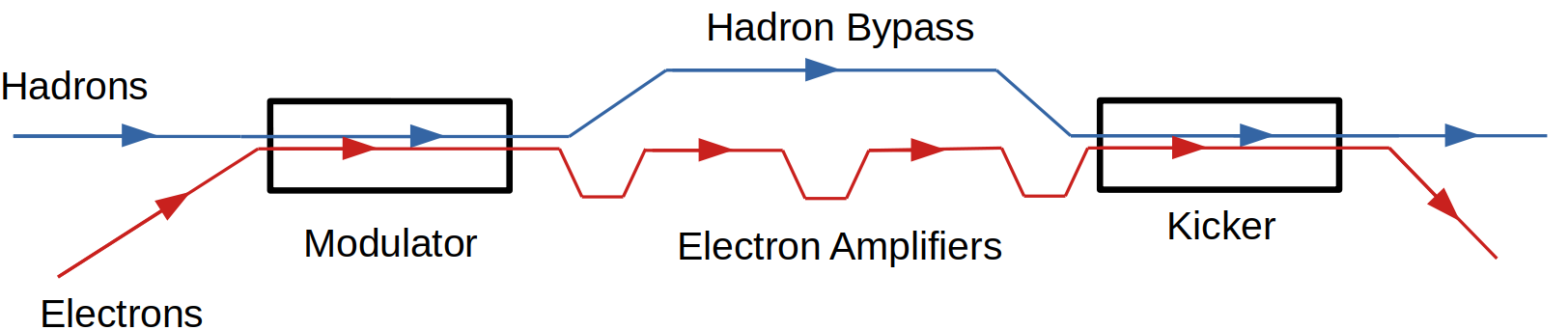
Figure 1: Schematic of the MBEC layout.

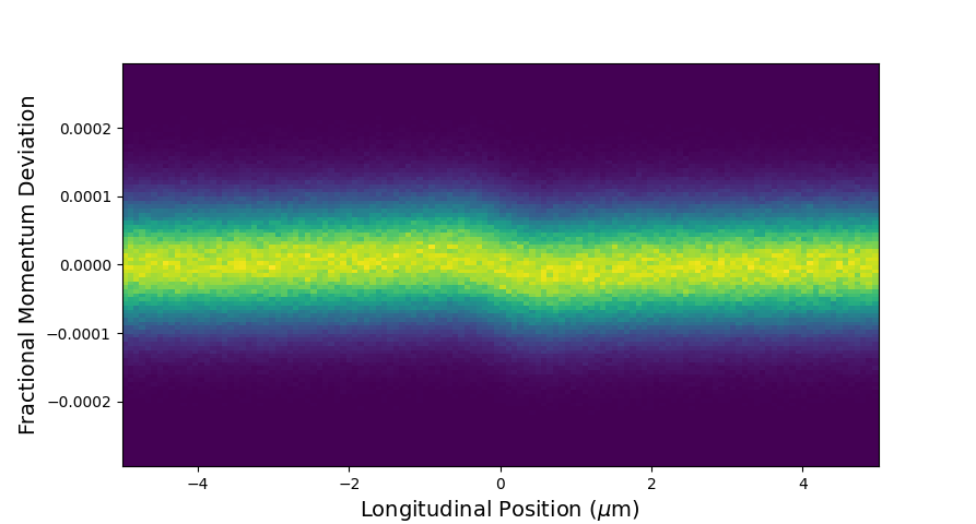
(a)

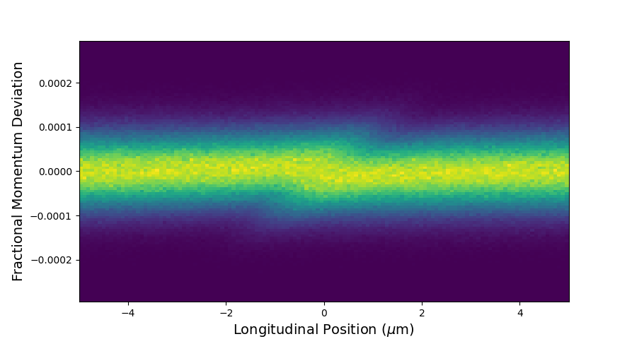
(b)

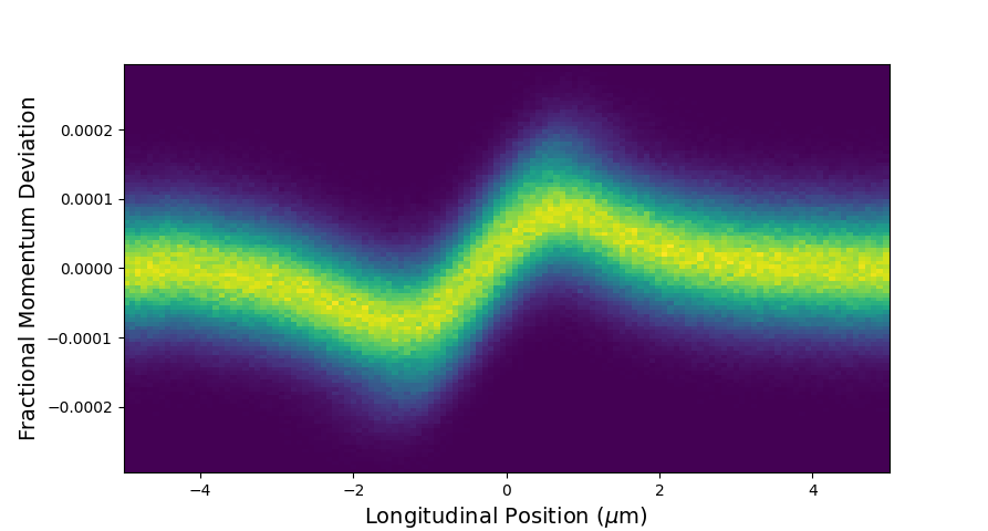
(c)

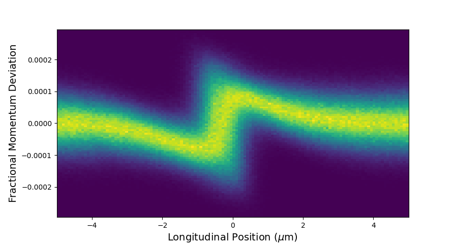
(d)

Figure 2: Evolution of the 2D phase space of the electron beam through an amplification section, seeded by 18 thousand protons in the modulator with longitudinal positions near the origin. The initial energy perturbation from the hadron seen in subfig. 2(a) is rotated into a density perturbation after the first chicane, as seen in subfig. 2(b). A partial plasma oscillation as the beam travels through the amplifier straight generates a significant energy modulation again, as in subfig. 2(c), and the next chicane rotates this into an amplified density perturbation, as in subfig. 2(d).

An important consideration in the operation of a cooler is diffusion; a given hadron sees not only its own wake, but also the wakes due to its neighbors, which provide a heating term partially counteracting the cooling. This has been previously discussed in Stupakov (2018); Stupakov and Baxevanis (2019); Baxevanis and Stupakov (2019, 2020). However, there is also a diffusion term originating in the noise in the electron beam; it will start off with initial energy and density fluctuations due to the Poisson statistics of discrete electrons and potentially some upstream instability, which will also be amplified within the cooler and provide energy kicks to the hadrons in the kicker. While Stupakov and Baxevanis (2019) provides some discussion of the electron diffusion, this ignores the effect of the electron-electron energy kicks in the modulator. Bergan et al. (2021) provides formulas related to this effect, but left their derivation vague, and provided no evidence of their accuracy. While direct particle-in-cell simulations, such as those discussed in Bergan (2021), allow for direct computation of electron noise, such methods are time-consuming, rendering an analytic model invaluable for fast optimization and design work.

In Section II of this paper, we will show an explicit derivation of the electron diffusion. In Section III, we compare the results of the theory to simulation. Section IV provides some practical considerations for how the electrons diffusion affects the cooler design and concludes.

II Theory

II.1 Electron Wakes

In order to determine the diffusion due to noise in the electron beam, it is first necessary to determine the effect which a single electron in the modulator will have on the energy kick received by a hadron in the kicker, which we can think of as the “electron wake.” The process of determining the single electron wake is complicated by the fact that it enters into the cooling process in two distinct ways. First, any given electron in the modulator will provide energy kicks to nearby electrons, inducing an energy fluctuation in a manner almost exactly the same as a hadron does. However, this electron will also propagate through the amplification sections itself; even if there were no modulator, the initial electron density modulation from shot noise alone would be amplified the same as one which had been induced due to energy kicks in the modulator.

We follow the approach of Stupakov (2018); Stupakov and Baxevanis (2019) and use the conventions developed therein. We model the electrons and hadrons as rigid charged discs, with the charge density falling off as Gaussians in the transverse directions whose standard deviations equal the horizontal or vertical beam sizes of the electron or hadron beams, as appropriate. We also assume a perfectly linear wake. Since the typical wake length scale of a few microns is much shorter than the few millimeter or few centimeter electron and hadron bunch lengths, we will assume the currents in both bunches are constant over any regions of interest. We note that the amplification process detailed in Stupakov and Baxevanis (2019) depends solely on the electron density modulations at the start of the first amplifier, after the first electron chicane. We will therefore end our analysis at this point, and use that paper’s machinery to get the kick to the hadrons in the kicker. The effect of the electron noise therefore only enters in determining the longitudinal electron density perturbation at the start of the first amplifier straight, $\delta n_{(a)}(z)$.

Let the electron distribution entering the modulator be described by the longitudinal phase-space density

$$f_{(m,e)}(z,\eta)=n_{e}F_{0}(\eta)+\delta f_{(m,e)}(z,\eta)$$ (1)

where $z$ is the longitudinal position within the bunch, $\eta$ is the electron’s fractional energy offset, $n_{e}$ is the constant component of the longitudinal electron density, $F_{0}(\eta)$ is the baseline electron energy distribution, and $\delta f_{(m,e)}$ is some perturbation to the above. Letting $\Delta\eta(z)$ be the energy kick an electron receives as a function of its longitudinal coordinate in the modulator, we may write the phase-space density at the start of the first amplifier straight, after passing through a chicane of strength $R_{1}$, as

$$f_{(a)}(z,\eta) =f_{(m,e)}(z-R_{1}\eta,\eta-\Delta\eta(z-R_{1}\eta))$$ (2)

$$=n_{e}F_{0}(\eta-\Delta\eta(z-R_{1}\eta))$$

$$+\delta f_{(m,e)}(z-R_{1}\eta,\eta-\Delta\eta(z-R_{1}\eta))$$

Subtracting off the background $n_{e}F_{0}(\eta)$, Taylor expanding the first term to $1^{st}$ order in $\Delta\eta$, and keeping only the $0^{th}$ order of the second term (since it is already assumed to be a small perturbation), we arrive at

$$\delta f_{(a)}(z,\eta) \approx-n_{e}F^{\prime}_{0}(\eta)\Delta\eta(z-R_{1}\eta)$$ (3)

$$+\delta f_{(m,e)}(z-R_{1}\eta,\eta)$$

and a corresponding frequency-space longitudinal density

$$\delta\hat{n}_{(a)}(k) \equiv\int_{-\infty}^{\infty}dze^{-ikz}n_{(a)}(z)$$ (4)

$$\equiv\int_{-\infty}^{\infty}d\eta\int_{-\infty}^{\infty}dze^{-ikz}f_{(a)}(z,\eta)$$

$$=\int_{-\infty}^{\infty}d\eta\int_{-\infty}^{\infty}dze^{-ikz}[-n_{e}F^{\prime}_{0}(\eta)\Delta\eta(z-R_{1}\eta)$$

$$+\delta f_{(m,e)}(z-R_{1}\eta,\eta)]$$

$$=-\int_{-\infty}^{\infty}d\eta e^{-ikR_{1}\eta}n_{e}F^{\prime}_{0}(\eta)\Delta\hat{\eta}(k)$$

$$+\int_{-\infty}^{\infty}d\eta\delta\hat{f}_{(a,\Delta\eta=0)}(k,\eta)$$

where we have defined appropriate frequency-space density functions. We have also defined $\delta f_{(a,\Delta\eta=0)}(z,\eta)\equiv f_{(m,e)}(z-R_{1}\eta,\eta)$ as the longitudinal phase-space density of the electron beam at the start of the first amplifier straight if there were no energy kicks in the modulator.

If we assume that $F_{0}(\eta)$ describes a Gaussian energy distribution with RMS fractional energy spread $\sigma_{\eta}$, we arrive at

$$\delta\hat{n}_{(a)}(k) =-ikR_{1}\int_{-\infty}^{\infty}d\eta e^{-ikR_{1}\eta}n_{e}F_{0}(\eta)\Delta\hat{\eta}(k)$$ (5)

$$+\delta\hat{n}_{(a,\Delta\eta=0)}(k)$$

$$=-ikR_{1}n_{e}e^{-k^{2}R_{1}^{2}\sigma_{\eta}^{2}/2}\Delta\hat{\eta}(k)+\delta\hat{n}_{(a,\Delta\eta=0)}(k)$$

We now need to calculate $\Delta\hat{\eta}(k)$. For the kick to the electrons due to the hadrons, this is provided by Eqtn. 54-56 of Stupakov (2018):

$$\Delta\hat{\eta}_{(eh)}(k)=\frac{2iZr_{e}L_{m}}{\gamma^{2}\Sigma}H_{(m,eh)}(\varkappa)\delta\hat{n}_{(m,h)}(k)$$ (6)

with

$$H_{(m,eh)}(\varkappa)\equiv\int_{0}^{\infty}d\xi\Phi_{(m,eh)}(\xi)\sin(\varkappa\xi)$$ (7)

and

$$\varkappa\equiv\frac{k\Sigma}{\gamma}$$ (8)

$\Sigma$ is just some normalization length scale, taken equal to the horizontal hadron beam size in the modulator. However, it cancels out everywhere, and can be changed with impunity. The other variables used are $Z$, the hadron charge; $r_{e}$, the classical electron radius; $L_{m}$, the modulator length; $\gamma$, the relativistic gamma factor; and $\delta\hat{n}_{(m,h)}(k)$, the frequency-space hadron density perturbation in the modulator. $\Phi_{(m,eh)}(\xi)$ is the electron-hadron interaction function in the modulator, defined based on Appendix C of Baxevanis and Stupakov (2019) as:

$$\Phi_{(m,eh)}(\xi)=\frac{4\xi}{\sqrt{\pi}}\int_{0}^{\infty}d\lambda\lambda^{2}$$ (9)

$$\times\frac{e^{-\lambda^{2}\xi^{2}}}{\sqrt{1+2\lambda^{2}(\Sigma_{x,h}^{2}+\Sigma_{x,e}^{2})/\Sigma^{2}}\sqrt{1+2\lambda^{2}(\Sigma_{y,h}^{2}+\Sigma_{y,e}^{2})/\Sigma^{2}}}$$

where the various $\Sigma$ terms are the horizontal and vertical beam sizes of the hadrons and electrons, labelled appropriately.

We may insert Eqtn. 9 into the definition of $H_{(m,eh)}(\varkappa)$ in Eqtn. 7. Using the antisymmetry of $\Phi$ to extend the $\xi$ integral from $-\infty$ to $\infty$ and doing it analytically, we obtain

$$H_{(m,eh)}(\varkappa)=\int_{0}^{\infty}d\lambda\frac{\varkappa}{\lambda}$$ (10)

$$\times\frac{e^{-\varkappa^{2}/4\lambda^{2}}}{\sqrt{1+2\lambda^{2}(\Sigma_{x,h}^{2}+\Sigma_{x,e}^{2})/\Sigma^{2}}\sqrt{1+2\lambda^{2}(\Sigma_{y,h}^{2}+\Sigma_{y,e}^{2})/\Sigma^{2}}}$$

For the kicks due to electron beam noise, we recognize that the physics is exactly the same, and so immediately write down

$$\Delta\hat{\eta}_{(ee)}(k) =-\frac{2ir_{e}L_{m}}{\gamma^{2}\Sigma}H_{(m,ee)}(\varkappa)\delta\hat{n}_{(m,e)}(k)$$ (11)

The changes from Eqtn. 6 are division by $-Z$ (the ratio of the hadron to electron charges), replacement of the hadron linear density by that of the electrons, and replacement of the electron-hadron $H$ function by the electron-electron version, which uses electron instead of hadron beam sizes in Eqtn. 10.

Putting Eqtn. 6 and 11 into Eqtn. 5, we obtain

$$\delta\hat{n}_{(a)}(k)= \frac{2Zr_{e}L_{m}}{\gamma^{2}\Sigma}kR_{1}n_{e}e^{-k^{2}R_{1}^{2}\sigma_{\eta}^{2}/2}$$ (12)

$$\times\bigg{(}H_{(m,eh)}(\varkappa)\delta\hat{n}_{(m,h)}(k)$$

$$-\frac{1}{Z}H_{(m,ee)}(\varkappa)\delta\hat{n}_{(m,e)}(k)\bigg{)}$$

$$+\delta\hat{n}_{(a,\Delta\eta=0)}(k)$$

From Stupakov and Baxevanis (2019), we see that the electron density at the kicker is equal to the electron density at the start of the first amplifier multiplied by the gain factors for the two amplifiers. These factors are denoted here by $G_{2}$ and $G_{3}$, with the number corresponding to the labelling of the associated electron chicane, and an expression for them is provided by Eqtn. 26 of Stupakov and Baxevanis (2019). Finally, it is evident that Eqtn. 6 describes the kick of the electron beam on the hadrons in the kicker if we multiply it by the ratio of the masses $m_{e}/m_{h}$, and change $L_{m}\rightarrow L_{k}$ (the kicker length), $H_{(m,eh)}\rightarrow H_{(k,eh)}$ (the electron-hadron interaction function in the kicker), and $\delta\hat{n}_{(m,h)}(k)\rightarrow\delta\hat{n}_{(k,e)}(k)$ (the electron density perturbation in the kicker). We arrive at an energy kick to the hadrons in the kicker:

$$\Delta\hat{\eta}_{(k,h)} =\frac{4iZ^{2}r_{e}^{2}L_{m}L_{k}m_{e}}{\gamma^{4}\Sigma^{2}m_{h}}kR_{1}n_{e}e^{-k^{2}R_{1}^{2}\sigma_{\eta}^{2}/2}$$ (13)

$$\times G_{2}G_{3}H_{(k,eh)}(\varkappa)\Big{(}H_{(m,eh)}(\varkappa)\delta\hat{n}_{(m,h)}(k)$$

$$-\frac{1}{Z}H_{(m,ee)}(\varkappa)\delta\hat{n}_{(m,e)}(k)\Big{)}$$

$$+\frac{2iZr_{e}L_{k}m_{e}}{\gamma^{2}\Sigma m_{h}}G_{2}G_{3}H_{(k,eh)}(\varkappa)\delta\hat{n}_{(a,\Delta\eta=0)}(k)$$

$$=\frac{4ir_{h}L_{m}L_{k}I_{e}}{I_{A}\gamma^{4}\Sigma^{2}\sigma_{\eta}}\varkappa q_{1}e^{-\varkappa^{2}q_{1}^{2}/2}G_{2}G_{3}H_{(k,eh)}(\varkappa)$$

$$\times\Big{(}H_{(m,eh)}(\varkappa)\delta\hat{n}_{(m,h)}(k)$$

$$-\frac{1}{Z}H_{(m,ee)}(\varkappa)\delta\hat{n}_{(m,e)}(k)\Big{)}$$

$$+\frac{2ir_{h}L_{k}}{Z\gamma^{2}\Sigma}G_{2}G_{3}H_{(k,eh)}(\varkappa)\delta\hat{n}_{(a,\Delta\eta=0)}(k)$$

where $r_{h}=\frac{Z^{2}e^{2}}{4\pi\epsilon_{0}m_{h}c^{2}}$ is the classical hadron radius, $I_{A}=\frac{ec}{r_{e}}\approx 17$kA is the Alfvén current, and $q_{1}\equiv\frac{R_{1}\sigma_{\eta}\gamma}{\Sigma}$

Note that three terms are summed here. The first corresponds to the wake due to the hadrons, which has been discussed extensively in Stupakov (2018); Stupakov and Baxevanis (2019); Baxevanis and Stupakov (2019). The second corresponds to the wake due to the electrons which operates on the same principles as the hadron wake - each electron provides an energy kick to neighboring electrons in the modulator, resulting in a perturbation to the electron density in the kicker which in turn causes an energy kick to the hadrons. The third term is due to the fact that, in the absence of energy kicks in the modulator, the initial shot noise in the electron beam will still be present at the start of the first amplifier, and so will be amplified and provide a kick to the hadrons in the kicker. This third term is covered in Stupakov and Baxevanis (2019). We need to keep two terms associated with the electrons because the electron shot noise enters into our calculations both by seeding energy perturbations in the modulator and in its “raw” form at the start of the first amplifier, forcing us to account for the unperturbed electron density modulations in both locations. To look at it another way, the hadrons can be approximated to leading order as stationary in the modulator, and so we only have to deal with their one dimensional distribution, while the electrons will change their longitudinal coordinate between the modulator and first amplifier due to their energy offsets, so that we have to consider the full 2-dimensional longitudinal phase space, necessitating the use of two wake functions.

We may translate the above into impedances with the definition

$$\Delta\hat{\eta}_{(k,h)}(k)=-\frac{r_{h}c}{\gamma} \big{(}Z_{h}(k)\delta\hat{n}_{(m,h)}(k)$$ (14)

$$+Z_{e,1}(k)\delta\hat{n}_{(m,e)}(k)$$

$$+Z_{e,2}(k)\delta\hat{n}_{(a,\Delta\eta=0)}(k)\big{)}$$

where

$$Z_{h}(k) =\frac{-4iL_{m}L_{k}I_{e}}{I_{A}c\gamma^{3}\Sigma^{2}\sigma_{\eta}}\varkappa q_{1}e^{-\varkappa^{2}q_{1}^{2}/2}$$ (15)

$$\times G_{2}G_{3}H_{(m,eh)}(\varkappa)H_{(k,eh)}(\varkappa)$$

$$Z_{e,1}(k) =\frac{4iL_{m}L_{k}I_{e}}{ZI_{A}c\gamma^{3}\Sigma^{2}\sigma_{\eta}}\varkappa q_{1}e^{-\varkappa^{2}q_{1}^{2}/2}$$

$$\times G_{2}G_{3}H_{(m,ee)}(\varkappa)H_{(k,eh)}(\varkappa)$$

$$Z_{e,2}(k) =\frac{-2iL_{k}}{Zc\gamma\Sigma}G_{2}G_{3}H_{(k,eh)}(\varkappa)$$

are the impedances for the hadrons, the self-induced electron density modulations, and the pre-existing electron density modulations, respectively.

II.2 Diffusion

We are now ready to calculate the diffusion, including the contribution from noise in the electron beam. For convenience, we move from frequency space to physical space, with the definition

$$w(z)=-\frac{c}{2\pi}\int_{-\infty}^{\infty}Z(k)e^{ikz}dk$$ (16)

so that

$$\Delta\eta_{(k,h)}(z)=\frac{r_{h}}{\gamma}\int_{-\infty}^{\infty}\big{[} w_{h}(z-z^{\prime})\delta n_{(m,h)}(z^{\prime})$$ (17)

$$+ w_{e,1}(z-z^{\prime})\delta n_{(m,e)}(z^{\prime})$$

$$+ w_{e,2}(z-z^{\prime})\delta n_{(a,\Delta\eta=0)}(z^{\prime})\big{]}dz^{\prime}$$

We assume that the electrons and hadrons entering the modulator have pure Poisson shot noise. Since the integral of each of the three wakes is zero, this implies that the average kick a hadron receives due to this noise is zero. It now remains to calculate the RMS kick strength. The average squared kick is given by

$$\Big{\langle}\Delta\eta_{(k,h)}^{2}\Big{\rangle}=\bigg{(}\frac{r_{h}}{\gamma}\bigg{)}^{2}\Bigg{\langle}\int_{-\infty}^{\infty}\int_{-\infty}^{\infty}dz^{\prime}dz^{\prime\prime}\big{[} w_{h}(z-z^{\prime})\delta n_{(m,h)}(z^{\prime})w_{h}(z-z^{\prime\prime})\delta n_{(m,h)}(z^{\prime\prime})$$ (18)

$$+ w_{e,1}(z-z^{\prime})\delta n_{(m,e)}(z^{\prime})w_{e,1}(z-z^{\prime\prime})\delta n_{(m,e)}(z^{\prime\prime})$$

$$+ w_{e,2}(z-z^{\prime})\delta n_{(a,\Delta\eta=0)}(z^{\prime})w_{e,2}(z-z^{\prime\prime})\delta n_{(a,\Delta\eta=0)}(z^{\prime\prime})$$

$$+ 2w_{e,1}(z-z^{\prime})\delta n_{(m,e)}(z^{\prime})w_{e,2}(z-z^{\prime\prime})\delta n_{(a,\Delta\eta=0)}(z^{\prime\prime})\big{]}\Bigg{\rangle}$$

We have ignored the hadron-electron cross-terms, since there is no correlation between those two beams. However, we do need to be careful about the cross-term from the two electron wakes. The longitudinal density perturbation for a particle in either beam can be written as

$$\delta n(z)=\sum_{i}\delta(z-z^{(i)})-n_{0}$$ (19)

where $n_{0}$ is the average particle density and $z^{(i)}$ is the position of the $i^{th}$ particle. Going forward, we will ignore the constant-background $-n_{e}$ term at the end, since the total integral of the wake is 0.

Putting this into the first term of Eqtn. 18, we obtain

$$\bigg{(}\frac{r_{h}}{\gamma}\bigg{)}^{2}\bigg{\langle}\sum_{i,j}w_{h}(z-z_{m}^{(i)})w_{h}(z-z_{m}^{(j)})\bigg{\rangle}$$ (20)

where $z_{m}^{(i)}$ refers to the position of particle $i$ in the modulator.

Since we assume white noise in the hadron beam, only the diagonal terms survive. We are then left with the sum over all hadron positions of the average squared hadron wake function, which can be rewritten as the integral

$$\bigg{(}\frac{r_{h}}{\gamma}\bigg{)}^{2}n_{h}\int_{-\infty}^{\infty}w^{2}_{h}(z^{\prime})dz^{\prime}$$ (21)

where $n_{h}$ is the mean linear hadron density.

The second and third terms of Eqtn. 18 can be simplified using an identical procedure. The fourth term requires some special care. Recall that $\delta n_{(m,e)}(z)$ is the density of electrons at the modulator, while $\delta n_{(a,\Delta\eta=0)}(z)$ is the electron longitudinal density at the first amplifier if we ignore the energy kicks in the modulator. If electron $i$ is located at position $z_{m}^{(i)}$ in the modulator, with fractional energy offset $\eta^{(i)}$, it will be at position $z_{m}^{(i)}+R_{1}\eta^{(i)}$ at the start of the first amplifier in the absence of modulator energy kicks. Using the same delta function and diagonalization arguments as above, we arrive at a simplification of the fourth term

$$2\bigg{(}\frac{r_{h}}{\gamma}\bigg{)}^{2}\bigg{\langle}\sum_{i}w_{e,1}(z-z_{m}^{(i)}) w_{e,2}(z-z_{m}^{(i)}-R_{1}\eta^{(i)})\bigg{\rangle}$$ (22)

$$=2\bigg{(}\frac{r_{h}}{\gamma}\bigg{)}^{2}n_{e}\int_{-\infty}^{\infty}dz^{\prime}\int_{-\infty}^{\infty}d\eta \frac{1}{\sqrt{2\pi}\sigma_{\eta}}e^{-\eta^{2}/2\sigma_{\eta}^{2}}$$

$$\times w_{e,1}(z^{\prime})w_{e,2}(z^{\prime}-R_{1}\eta)$$

where we have assumed a Gaussian fractional energy spread of RMS $\sigma_{\eta}$ and longitudinal electron bunch density of $n_{e}$.

For a wake scale of $\sim 1\mu$m, a 6cm hadron beam of $6.9\times 10^{10}$ protons, and a 1nC beam of electrons with bunch length of roughly 1cm, we expect on the order of several hundred thousand particles from each beam to contribute to the diffusion term. Using the central limit theorem, the diffusive kick which a proton receives each turn can be approximated as being drawn from a Gaussian distribution with a mean of $0$ and a variance given by

$$\Big{\langle}\Delta\eta_{(k,h)}^{2}\Big{\rangle}=\bigg{(}\frac{r_{h}}{\gamma}\bigg{)}^{2}\int_{-\infty}^{\infty} dz^{\prime}\bigg{(}n_{h}w^{2}_{h}(z^{\prime})$$ (23)

$$+ n_{e}w^{2}_{e,1}(z^{\prime})+n_{e}w^{2}_{e,2}(z^{\prime})$$

$$+ 2n_{e}\int_{-\infty}^{\infty}d\eta\frac{1}{\sqrt{2\pi}\sigma_{\eta}}e^{-\eta^{2}/2\sigma_{\eta}^{2}}$$

$$\times w_{e,1}(z^{\prime})w_{e,2}(z^{\prime}-R_{1}\eta)\bigg{)}$$

This procedure for simulating the diffusive kicks as random numbers drawn from an appropriate distribution is similar to the methods used in Wang (2019) to model IBS in a simulation of coherent electron cooling and in Wang et al. (2021) to model diffusion in a simulation of optical stochastic cooling.

III Simulation

In order to verify the above calculations, we turn to a one-dimensional particle-in-cell (PIC) simulation, described previously in Bergan (2021) and Bergan et al. (2022). We use parameters based on those currently planned for cooling 275GeV protons at the EIC, shown in Tab. 1. However, in order to avoid nonlinear effects, we use only one amplification section, ie, we place the kicker immediately after the second electron chicane. We also track through the modulator and kicker in a single step to avoid the impact of plasma oscillations in those regions, with the effective $R_{56}$ of the modulator length added to the $R_{56}$ of the first chicane when obtaining the theory wakes. This code creates the same number of electrons within a 10$\mu$m section of the beam as would be expected from the peak electron bunch density. These have a uniform longitudinal distribution and Gaussian momentum distribution. We also generate $10^{5}$ proton macroparticles within the same region with uniform longitudinal and Gaussian momentum distributions, each having the charge of 6.8 real protons. Since noise adds in quadrature, this is statistically equivalent to having the full $4.6\times 10^{6}$ protons expected within a 10$\mu$m length at the bunch center. Particles are propagated through the cooler with a simple kick-drift model. The kick is calculated using the usual particle-in-cell (PIC) formalism with periodic boundary conditions, 128 longitudinal bins of length $\sim$78nm, and with the electron-electron and electron-proton forces making use of the disc-disc interaction functions described in Stupakov (2018); Stupakov and Baxevanis (2019); Baxevanis and Stupakov (2019) and discussed in Eqtn. 6 - 11 of this paper. We work convert these to fractional momentum kicks by $\Delta\delta=\Delta\eta/\beta^{2}$, where $\delta$ is the particle’s fractional momentum deviation and $\beta\approx 1$ is the relativistic beta function. The longitudinal coordinates are then updated as $z\rightarrow z+\Delta s\delta/\gamma^{2}$, where $\Delta s$ is the step length and $\gamma$ is the relativistic gamma function common to both particle species. The chicanes are modelled as simple point elements translating the particles’ longitudinal coordinates by $z\rightarrow z+R_{56}\delta$.

Table 1: Parameters for Longitudinal and Transverse Cooling

Geometry
Modulator Length (m)	33
Kicker Length (m)	33
Number of Amplifier Straights	2
Amplifier Straight Lengths (m)	49
Proton Parameters
Energy (GeV)	275
Protons per Bunch	6.9e10
Proton Bunch Length (cm)	6
Proton Fractional Energy Spread	6.8e-4
Proton Emittance (x/y) (nm)	11.3 / 1
Horizontal/Vertical Proton Betas in Modulator (m)	21 / 20
Horizontal/Vertical Proton Dispersion in Modulator (m)	0.002 / 0.067
Horizontal/Vertical Proton Dispersion Derivative in Modulator (m)	0.030 / -0.005
Horizontal/Vertical Proton Betas in Kicker (m)	21 / 20
Horizontal/Vertical Proton Dispersion in Kicker (m)	0.002 / 0.067
Horizontal/Vertical Proton Dispersion Derivative in Kicker (m)	0.030 / -0.005
Proton Horizontal/Vertical Phase Advance (rad)	3.17 / 4.76
Proton $R_{56}$ between Centers of Modulator and Kicker (mm)	1.348
Electron Parameters
Energy (MeV)	150
Electron Bunch Charge (nC)	1
Electron Peak Current (A)	13
Electron Fractional Slice Energy Spread	1e-4
Electron Normalized Emittance (x/y) (mm-mrad)	2.8 / 2.8
Horizontal/Vertical Electron Betas in Modulator (m)	21 / 21
Horizontal/Vertical Electron Betas in Kicker (m)	8 / 8
Horizontal/Vertical Electron Betas in Amplifier Straights (m)	5 / 5
$R_{56}$ in First Electron Chicane (mm)	12.0
$R_{56}$ in Second Electron Chicane (mm)	-6.7
$R_{56}$ in Third Electron Chicane (mm)	-6.8
Cooling Times
Horizontal/Vertical/Longitudinal IBS/Beam-Beam Times (hours)	2.0 / 5.0 / 2.9
Horizontal/Vertical/Longitudinal Cooling Times (hours)	0.9 / 1.9 / 1.2

In Fig. 3, we show the kick to a test proton in the kicker due to initial proton and electron noise in the modulator. We compare this to a theory curve made by convolving the initial proton and electron distributions with the wake functions derived from the impedances of Eqtn. 15. We see that the theory reproduces the simulated result quite well. In order to focus on the electron wake, we rerun the simulation with no protons in the modulator, with the result shown in Fig. 4. Again, good agreement with simulation is observed.

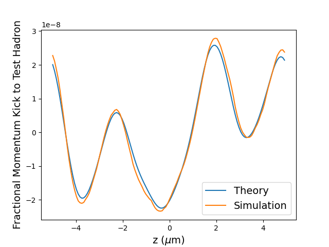
Figure 3: Fractional momentum kick to a proton in the kicker due to initial proton and electron noise in the modulator. Good agreement between theory and simulation is observed.

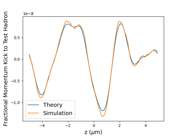
Figure 4: Fractional momentum kick to a proton in the kicker due to only initial electron noise in the modulator. Good agreement between theory and simulation is observed.

As a check of the necessity of both terms in the electron wake, we compute the electron theory curve using only the electron wakes corresponding to $Z_{e,1}(k)$ and $Z_{e,2}(k)$ individually, with the results shown in Fig. 5 and 6, respectively. We see that using $Z_{e,1}(k)$ alone shows noticeable discrepancies from the simulated result, and using $Z_{e,2}(k)$ alone produces theory kicks which have very little correspondence to what is seen in simulation. Both terms are therefore necessary for properly understanding the evolution of the beam.

Figure 5: Fractional momentum kick to a proton in the kicker due to only initial electron noise in the modulator. The theory here only uses the middle impedance in Eqtn. 15, and differs noticeably from the simulated result.

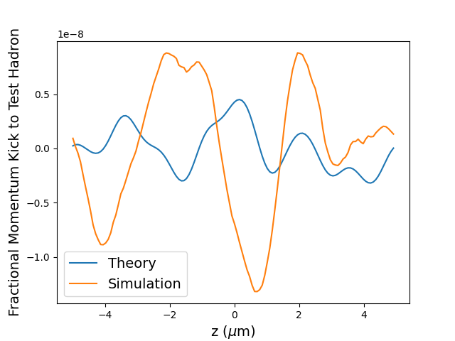
Figure 6: Fractional momentum kick to a proton in the kicker due to only initial electron noise in the modulator. The theory here only uses the final impedance in Eqtn. 15, and is very different from the simulated result.

We finally turn to the question of diffusion. We run the simulation 1000 times, starting with only electron noise, and record the fractional momentum kick which a test proton would receive in the kicker in each case at 128 locations over a 10$\mu$m length of beam. A histogram of the results is shown in Fig. 7, along with the expected Gaussian distribution with RMS value given by Eqtn. 23. The RMS kick received in simulation is $6.04\times 10^{-9}\pm 0.05\times 10^{-9}$, similar to, but slightly above, the value of $5.81\times 10^{-9}$ obtained from Eqtn. 23. Since the simulation includes additional physics, such as keeping the full longitudinal phase-space distribution at the start of the amplifier rather than projecting to the spatial plane, exact agreement is not expected.

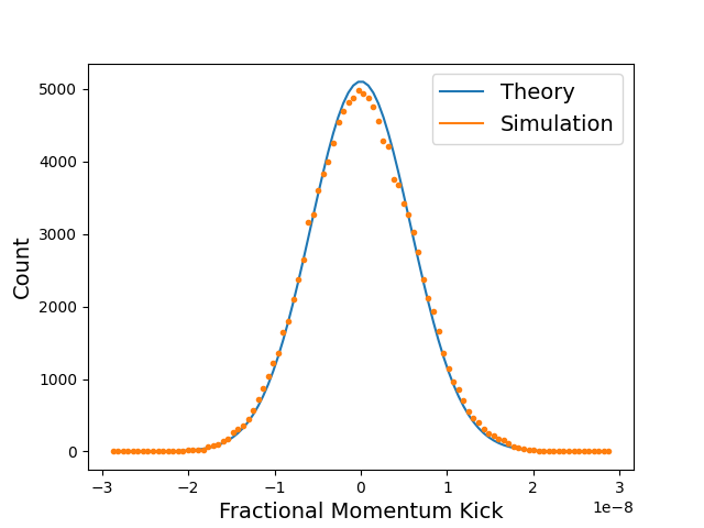
Figure 7: Histogram of fractional momentum kicks to a proton in the kicker as obtained from the simulation and compared to the theoretical Gaussian distribution. Decent agreement is observed, although additional physics included in the simulation does lead to slight discrepancies.

If we recompute the theory value either ignoring the cross-term of Eqtn. 23 or assuming that the two separate electron wakes can be simply added, we obtain values of $7.77\times 10^{-9}$ and $4.31\times 10^{-9}$, respectively, showing that the form of the cross-term we have derived is both necessary and consistent with simulation. For comparison, the theoretical RMS fractional momentum kick from the proton noise is $11.3\times 10^{-9}$, so that the electron contribution to diffusion cannot be neglected.

IV Conclusion

We have derived formulas for the diffusion expected in a microbunched electron cooling system due to initial shot noise in the electron beam. Along the way, we have shown how to obtain the response to an arbitrary electron distribution in the modulator. For a reasonable set of parameters, this can be comparable to the proton noise. An examination of Eqtn. 15 shows that if the $R_{56}$ across the first chicane is negative, the two electron impedances have the same sign, while a positive $R_{56}$ will give the two impedances with opposite signs. Physically, a negative $R_{56}$ will give the electrons an effective negative mass, leading to additional clumping, while a positive $R_{56}$ results in electrostatic repulsion pushing electrons apart. The latter option is greatly preferred in the design of a cooler, since it will cause some cancellation in the electron noise.

V Acknowledgements

This work was supported by Brookhaven Science Associates, LLC under Contract No. DE-SC0012704 with the U.S. Department of Energy. I would also like to thank Erdong Wang, Michael Blaskiewicz, and Panagiotis Baxevanis for useful discussions.

References

- Willeke et al. (2021) F. Willeke et al., Electron Ion Collider Conceptual Design Report 2021, Tech. Rep. (Brookhaven National Laboratory and Thomas Jefferson National Accelerator Facility, 2021).
- Ratner (2013) D. Ratner, Phys. Rev. Lett. 111, 084802 (2013).
- Stupakov (2018) G. Stupakov, Phys. Rev. Accel. Beams 21, 114402 (2018).
- Stupakov and Baxevanis (2019) G. Stupakov and P. Baxevanis, Phys. Rev. Accel. Beams 22, 034401 (2019).
- Baxevanis and Stupakov (2019) P. Baxevanis and G. Stupakov, Phys. Rev. Accel. Beams 22, 081003 (2019).
- Baxevanis and Stupakov (2020) P. Baxevanis and G. Stupakov, Phys. Rev. Accel. Beams 23, 111001 (2020).
- Bergan et al. (2021) W. F. Bergan, P. Baxevanis, M. Blaskiewicz, and E. Wang, in Proceedings of IPAC 2021 (Campinas, Brazil, 2021) pp. 1819–1822, TUPAB179.
- Bergan (2021) W. F. Bergan, in Proceedings of IPAC 2021 (Campinas, Brazil, 2021) pp. 1823–1826, TUPAB180.
- Wang (2019) G. Wang, Phys. Rev. Accel. Beams 22, 111002 (2019).
- Wang et al. (2021) S. T. Wang, M. B. Andorf, I. V. Bazarov, W. F. Bergan, V. Khachatryan, J. M. Maxson, and D. L. Rubin, Phys. Rev. Accel. Beams 24, 064001 (2021).
- Bergan et al. (2022) W. F. Bergan, M. Blaskiewicz, and G. Stupakov, Phys. Rev. Accel. Beams 25, 094401 (2022).