Resolution Limit of Single-Photon LiDAR
Abstract
Single-photon Light Detection and Ranging (LiDAR) systems are often equipped with an array of detectors for improved spatial resolution and sensing speed. However, given a fixed amount of flux produced by the laser transmitter across the scene, the per-pixel Signal-to-Noise Ratio (SNR) will decrease when more pixels are packed in a unit space. This presents a fundamental trade-off between the spatial resolution of the sensor array and the SNR received at each pixel. Theoretical characterization of this fundamental limit is explored. By deriving the photon arrival statistics and introducing a series of new approximation techniques, the Mean Squared Error (MSE) of the maximum-likelihood estimator of the time delay is derived. The theoretical predictions align well with simulations and real data.
1 Introduction
Single-photon LiDAR has a wide range of applications in navigation and object identification [33, 27, 22, 25, 31, 26]. By actively illuminating the scene with a laser pulse of a known shape, we measure the time delays of single photons upon their return, which correspond to the distance of the object [4, 20, 37]. The advancement of photo detectors has significantly improved the resolution of today’s LiDAR [43, 34, 9, 18, 41, 42, 16]. Moreover, algorithms have shown how to reconstruct both the scene reflectivity and 3D structure [37, 21, 30, 23, 2, 39, 44, 45, 7, 17, 24].
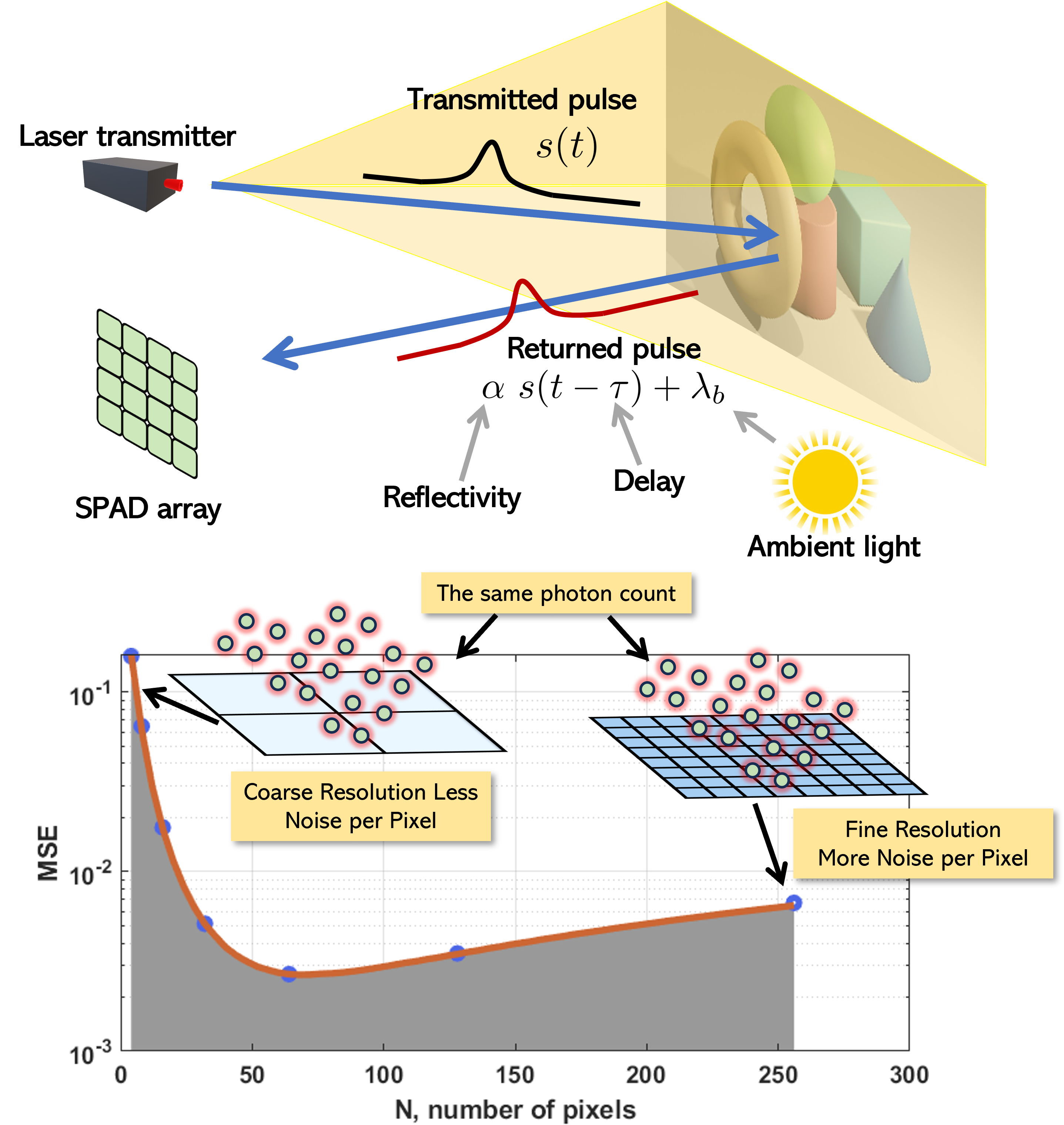
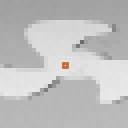
As an imaging device, a photodetector used in LiDAR faces similar problems as any other CCD or CMOS pixels. Packing more pixels into a unit space decreases the SNR because the amount of photon flux seen by each pixel diminishes [13]. This fundamental limit is linked to the stochastic nature of the underlying Poisson arrival process of the photons [38, 12]. Unless noise mitigation schemes are employed [2, 23, 32, 15], there is a trade-off between the number of pixels one can pack in a unit space and the SNR we will observe at each pixel. The situation can be visualized in Fig. 1, where we highlight the phenomenon that if we use many small pixels, the spatial resolution is good but the per pixel noise caused by the random fluctuation of photons will be high. The bias and variance trade-off will then lead to a performance curve that tells us how the accuracy of the depth estimate will behave as we vary the spatial resolution.
The goal of this paper is to rigorously derive the above phenomenon. In particular, we want to answer the following question:
The theoretical analysis presented in this paper is unique from several perspectives:
-
•
Beyond Single Pixel. The majority of the computer vision papers in single-photon LiDAR are algorithmic. Few papers have theoretical derivations, but they all focus on a single pixel [2, 23, 32, 15], of which the foundation can be traced back to the original work of Bar-David (1969) [3]. Our paper departs from these results by generalizing the mean square estimation to an array of pixels.
-
•
New Proof Techniques. A brute force derivation of the mean squared error is notoriously difficult. We overcome the hurdles by introducing a series of new theoretical approximation techniques in terms of modeling depth, approximating pixels, and utilizing convolutions.
-
•
Closed-form Results. Under appropriate assumptions about the scene and sensors, our result has a simple interpretable closed-form expression that provides an excellent match with the practical scenarios in both real-world and simulated experiments.
2 Background: Photon Arrival Statistics
In this section, we discuss the mathematical preliminaries. Our result is based on Bar-David [3] which precedes many of the more recently published work [32, 14, 38]. For notation simplicity, our models are derived in 1D. Moreover, to make the main text concise, proofs of theorems are presented in the supplementary material.
2.1 Pulse Model
Let [m/s] be the speed of light, and let be the distance [m] of the object at coordinate . Hence, the total time [s] for the pulse to travel forward and then back is . We assume that is a continuous-space function with a continuous amplitude.
The laser pulse is defined as a symmetric time-invarying function . Given a delay , the shifted pulse is .
For simplicity, we ignore the boundary conditions by assuming that the observation interval is significantly larger than the width of the pulse, i.e., . Moreover, We assume that the delay lies well inside the observation interval, and the pulse is normalized so that
| (2) |
As the pulse reaches an object and is reflected back to the receiver, the received pulse takes the form of
| (3) |
In this equation, denotes the reflectivity of the object. For simplicity, we assume that is a constant. The constant denotes the background flux due to ambient light. The energy carried by is measured by
| (4) |
Which can be obtained by inserting Eq. 3 into the integrand shown in Eq. 4, and then using Eq. 2 to evaluate the integral.
2.2 Time of Arrival
Given , we assume that number of time stamps are generated over . Denote these time stamps as , where . The joint distribution of and is as follows.
The number is a random variable. The probability mass function of can be computed by marginalizing the joint distribution.
If , then there is no occurrence in . In this case, the probability is defined as
| (7) |
The conditional probability of seeing given can be obtained by taking the ratio of the joint distribution and , yielding the following result.
| (8) |
The other conditional probability of seeing given is 1. Putting these together, we can show that
| (9) |
We can show that the integration of over the entire sample space is 1:
2.3 Sampling from
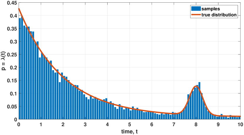
When the pulse is Gaussian, Monte Carlo simulations of the time stamps can be performed in a two-step process:
-
•
Step 1: Determine the number of samples . This can be done by recognizing that the total energy of the pulse is . The total number of samples is a Poisson random variable such that . However, since the two summands of are independent, Raikov theorem states that can be decomposed into a sum of two independent Poisson random variables. Thus, the number of samples is determined based on
(11) We let .
-
•
Step 2: Draw samples from and samples from a uniform distribution of a PDF:
The overall set of samples is .
As we can see, the distribution of the samples is nothing but the shape of the pulse. This is consistent with the literature where we draw a random number representing the height of each histogram bin. In our sampling procedure, we draw the time stamps without quantizing them into bins. For pulses of an arbitrary shape, we can perform an inverse CDF technique outlined in the supplementary material.
2.4 Assumptions For Theoretical Analysis
The goal of this paper is to derive closed-form results. As such, a series of assumptions are required to minimize the notational burden. Our assumptions are summarized below:
-
•
We do not assume any dark current. In the supplementary material, we have a discussion about the dark current effects.
-
•
We assume that is a constant. To relax this assumption, we can replace with in the proof. However, the final equation will involve an integration over .
- •
-
•
Self-excitation process. Prior work such as [32] and [14] use self-excitation process (a variant of the Markov chain) to model the photon arrivals [38]. While this is accurate, deriving closed-form expressions is infeasible. Since we do not assume any dead-time, we follow Bar-David’s inhomogeneous Poisson process [3] instead.
-
•
Single-bounce and no multiple path. This is a standard assumption in LiDAR theory.
3 MSE Analysis
3.1 Single-Pixel MSE
To quantify the performance of a LiDAR pixel, we recall that the decision process involves estimating the delay given the measurements . Therefore, we need to specify the estimation procedure. Based on the estimates, we can then discuss the performance by evaluating the variance of the estimate.
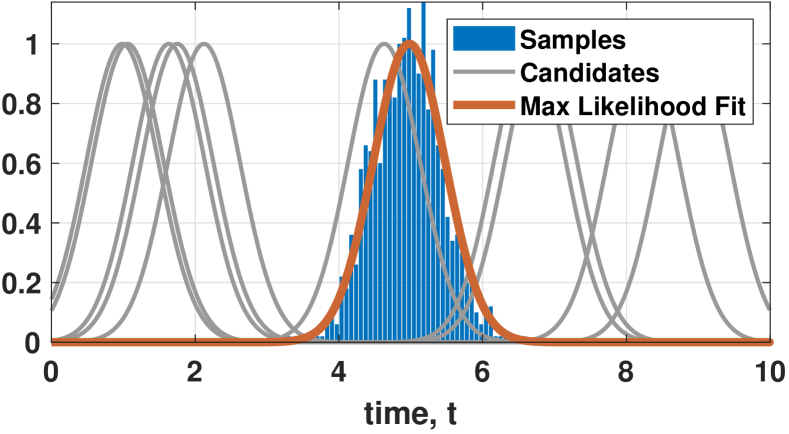
Maximum-Likelihood Estimation (MLE). When no knowledge about is known a priori, we use MLE [19, 37]. MLE has been thoroughly exploited in single-depth estimation problems [2]. Given the measured time stamps , we consider the log-likelihood
Since the variable in the ML estimation is the time shift, the optimization can be solved by running a matched filter. Given the shape , we shift the pulse left and right until we see the best match with the data. Fig. 2 shows a pictorial illustration.
If is the ML estimate, it is necessary that
| (12) |
This result is used in the implementation. Details can be found in the supplementary material.
MSE calculation.When denotes the true time of arrival, the Taylor expansion of will give us
Substituting , and using the fact that because is the maximizer, we can show that
Therefore, the error is . By using this result, the variance of the estimate can be shown as follows.
3.2 Space-Time Model
Continuous . Our resolution-noise trade-off analysis requires a model of an array of pixels. To this end, we need to generalize from a single time delay to a function of time of arrivals where is the spatial coordinate. Thus, at every location , and given the pulse shape , the ideal return pulse is
| (14) |
Fig. 3 shows a typical where the time delay is translated to a space-time signal with a Gaussian pulse at every . The discretization of will play a key role in our analysis.
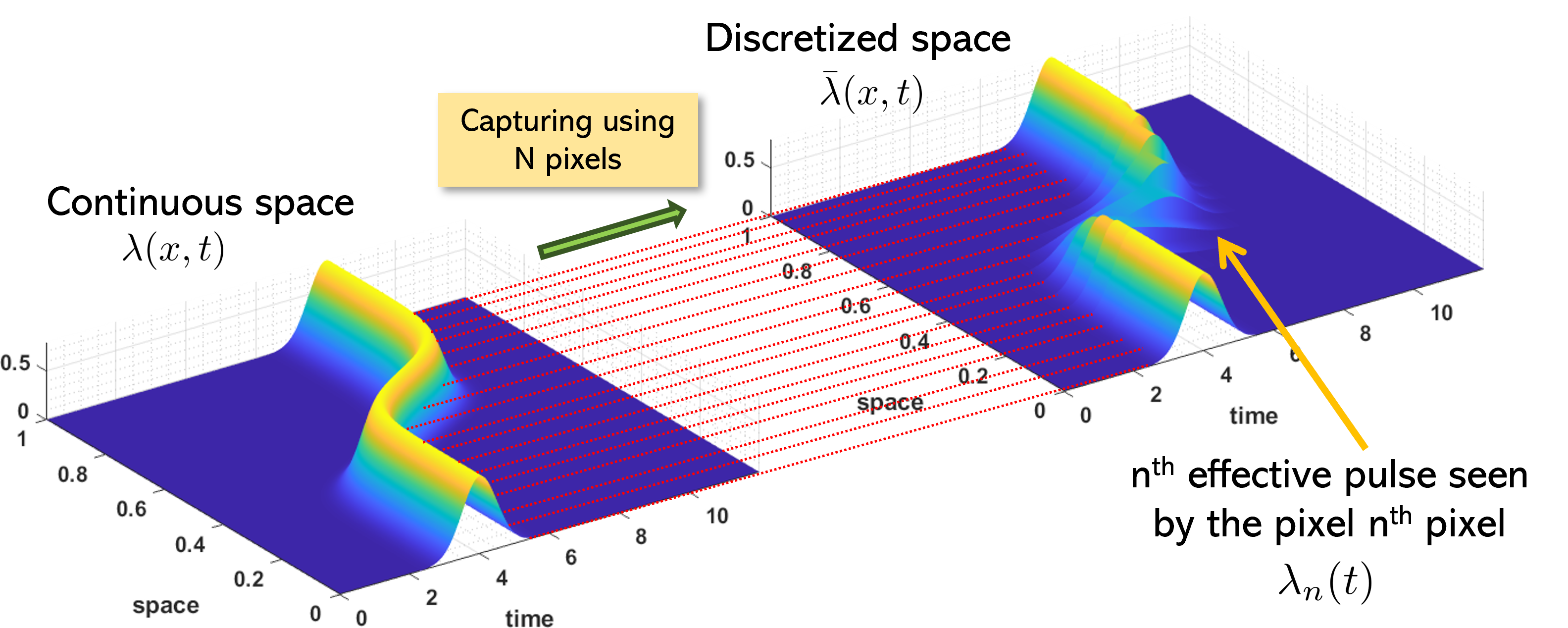
Observing through pixels. Suppose that we allocate pixels in the unit space to measure the returned time of arrivals. These times of arrivals are generated according to the joint distribution specified in Eq. 3. However, since at the pixel the function occupies the interval , we can define the effective return pulse by absorbing the coordinate through integration. Specifically, we define as
| (15) |
The resulting space-time approximation of is thus a piecewise function
| (16) |
where is a boxcar function defined as
| (17) |
The definition here is consistent with how the spatial-oversampled quanta image sensor was defined [46, 10].
Remark 1: Can we approximate instead? By looking at Eq. 15, it is tempted to think that we can approximate via a piecewise constant function
| (18) |
where
| (19) |
This will give us a plausible candidate for :
| (20) |
However, the problem with this approximation is that physically it is invalid. As light propagates, the energy carried by the wave follows the “scattering” process via the superposition of the electromagnetic field [6]. When energy is distributed from the source, we need to integrate and not .
3.3 New Approximation Techniques
While Eq. 15 is a physically valid way to perform spatial discretization, it does not have a simple analytic expression. For example, when and , if we plug a Gaussian pulse into Eq. 15, we will need to evaluate the integral
Since is a function of , it is impossible to arrive at a closed-form expression.
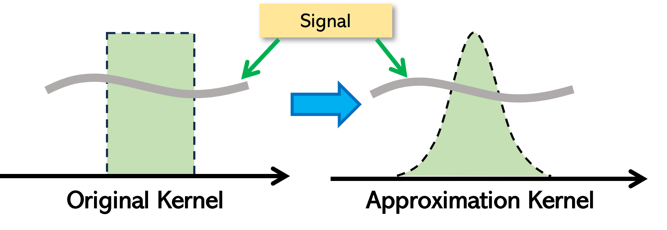
Our plan of deriving the theoretical bound involves several steps. At the core of our proof technique is the approximation of the boxcar function using a Gaussian kernel, as illustrated in Fig. 4. If we assume that the pulse is also a Gaussian, then a convolution of two Gaussians will remain a Gaussian. This will substantially improve the tractability of our equations.
Approximation 1: Linearize . We approximate the time of arrival function by a piecewise linear function. Suppose that there are pixels in . We define the mid point of each interval as
Expanding around will give us
| (21) |
Thus, for the entire , is approximated by
| (22) |
where is the boxcar function defined in Eq. 17.
Approximation 2: Replace boxcar by Gaussian. The second approximation is to give up the boxcar function because it does not allow us to derive a closed-form expression of . We replace it with a Gaussian :
| (23) |
However, if we want to approximate a boxcar function (with width ) by a Gaussian (with a standard deviation ), what should be the relationship between and so that the approximation is optimized? The answer is .
If there are pixels in , then the width of each pixel is . This means that has a width of . Therefore, the standard deviation of the shifted Gaussian is .
Approximation 3: Replace projection by convolution. One of the difficulties in Eq. 15 is the integration over the spatial interval. With the introduction of the Gaussian kernel, we replace the projection step by a spatially invariant convolution:
The resulting can then be determined as the value of at the mid point of each pixel interval, i.e.,
| (25) |
The following theorem summarizes the result of this series of approximations:
The biggest difference between Eq. 26 and Eq. 20 is the standard deviation of the Gaussian. In Eq. 20, the pulse width is always . Thus, the shape of the Gaussian is never changed no matter which pixel we consider. This problem is fixed in Eq. 26 where the standard deviation now depends on three things: (i) the temporal pulse width , (ii) the width of the pixel , (iii) the first derivative of the time of arrival function .
3.4 Derivation of the MSE
Bias-Variance Decomposition. We are now in the position to derive the overall MSE. The MSE is measured between the true function and the reconstructed function :
| (27) |
In this equation, the reconstructed function is a piecewise constant function defined by
where is the ML estimate of the time of arrival at the pixel, and is the boxcar function.
As will be shown in the supplementary material, the MSE defined Eq. 27 can be decomposed into bias and variance:
The bias measures how much resolution will drop when we use piecewise constant function to approximate the continuous . The variance measures the noise fluctuation caused by the random ML estimate .
Main Theoretical Result. The main result is stated in the theorem below.
When deriving this main result, we assume that the pulse is Gaussian and the floor noise is zero. We will relax these assumptions in the supplementary material to consider more realistic situations.
Significance of Theorem 4. The main result is the first closed-form expression about the noise-resolution trade-off that we are aware of. As we will demonstrate in the experiment section, this simple formula matches well with the Monte Carlo simulation, albeit with minor numerical precision errors.
The closed-form expression in Theorem 4 offers many important insights about the behavior of the problem.
-
•
: Since is the total flux of the scene, a large will generate more time stamps which will in turn improve the variance. has no impact on the bias.
-
•
: The pulse width determines the uncertainty of the time of arrivals, which affects the variance. does not affect the bias because the bias is independent of .
-
•
: The slope of specifies “how difficult” the scene is. In the easiest case where the scene is flat so that , the bias term drops to zero. If the slope is large, both bias and variance will suffer.
-
•
: The parameter is a modeling constant. can be considered as a proxy to any diffraction limit caused by the optical system. A large point spread function of the optics will result in a large .
4 Experiments
4.1 Simulated 1D Experiment
We consider multiple 1D ground truth time of arrival functions outlined in the supplementary material Sec. 9. The configurations can be found in Tab 1, also in the supplementary material.
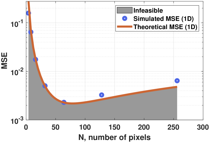
Simulation. During simulation, we construct a space-time function with a very fine-grained spatial grid. At each in the grid, there is a pulse function . We integrate for for each interval to obtain the effective pulse . random time stamps are drawn from the inverse CDF of , where is a Poisson random variable with a rate . The time stamps (per each ) will give us an estimate , which is then used to construct the reconstructed delay profile . We numerically compute the MSE for this .
Theory. The theoretical prediction follows the equation described in Theorem 4. This is a one-line formula.
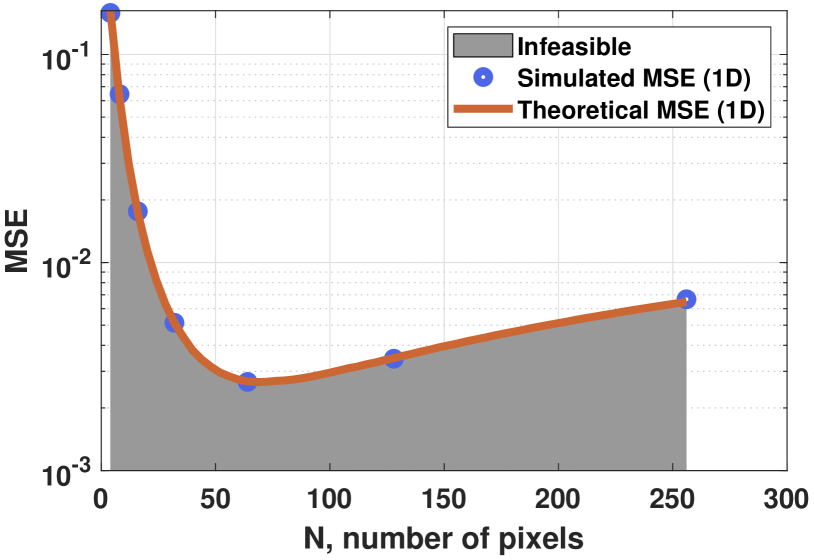
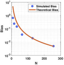
Result. The result of our experiment is reported in Fig. 5. As evident from the figure, the theoretical prediction matches very well with the simulation. The optimal number of pixels for this particular problem is around .
4.2 Analysis of Variance
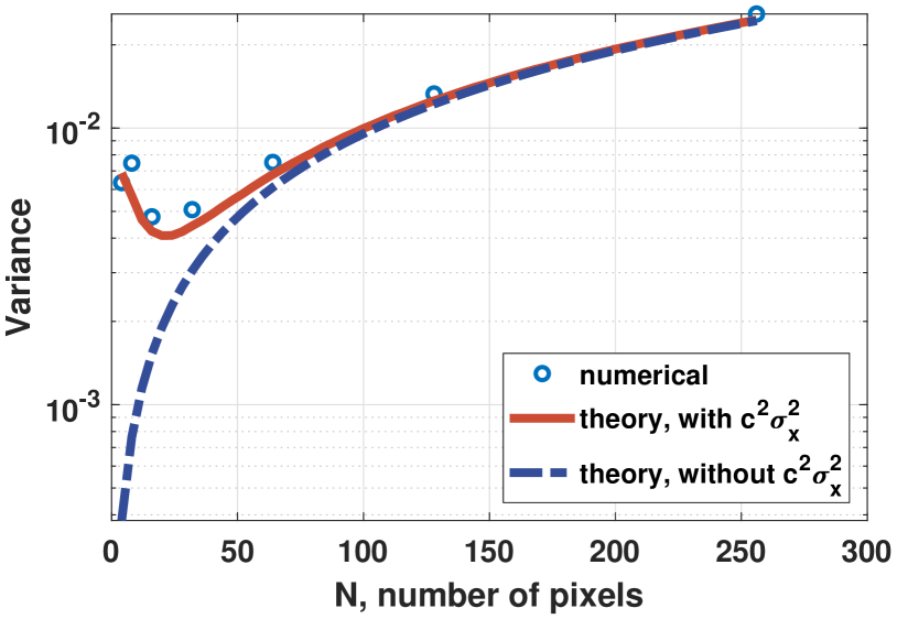
Our second experiment concerns about the validity of the approximations. Suppose we take a “lazy” route by using the “cheap” approximation outlined in Eq. 20. Then, under the condition that is Gaussian and , Theorem 2 will give us (via Example 3)
| (29) |
Compared with Theorem 4, the term is omitted. For the particular example shown in Fig. 5, we show in Fig. 6 a side-by-side comparison when the term is included and not included. It is clear from the figure that only the one with included can match with the simulation.
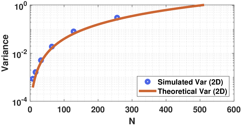
4.3 Simulated 2D Experiment
Simulation. For 2D experiments, we use a ground truth depth map to generate the true time of arrival signal . Then, following a similar procedure outlined for the 1D case, we generate time stamps according to the required spatial resolution. For simplicity, we assume that the pulses are Gaussian, and that there is no noise floor. A piecewise constant 2D signal is reconstructed and the MSE is calculated.
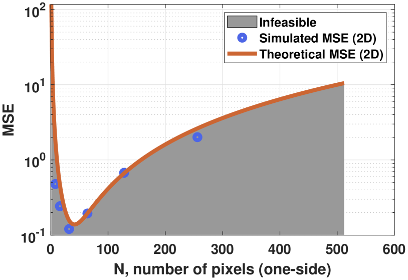
Theory. The derivation of the theoretical MSE is outlined in the supplementary material Sec 14. Summarizing it here, the MSE is (with being the number of pixels in one direction)
| (30) |
where is the average gradient of the 2D time of arrival function.
 |
 |
 |
 |
 |
 |
 |
 |
 |
Result. The result is outlined in Fig. 7. As we can see, the theoretical MSE again provides an excellent match with the simulated MSE.
4.4 Real 2D Experiment
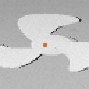
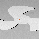
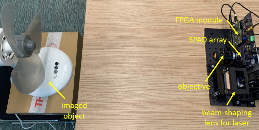
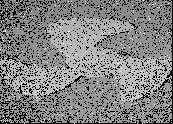
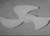
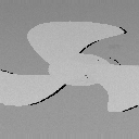
In this experiment we analyze the real SPAD data collected by a sensor reported in [18]. The indoor scene consists of a static fan with a flat background, which is flood-illuminated using a picosecond pulsed laser source (Picoquant LDH series 670 nm laser diode with 1nJ pulse energy, operated with 25 MHz repetition rate). An f/4 objective was used in front of the SPAD, and binary time stamp frames (with a maximum of a single time stamp per pixel) were captured with an exposure time of 1 ms per frame. A total of 10,000 time stamps with a timing resolution of 35ps were thereby collected for each pixel. Pre-processing is performed to remove outliers. More descriptions of how this is done can be found in the supplementary material. The outcomes of the real 2D experiment are depicted in Fig. 8, whereas the schematic diagram of the experimental setup is shown in Fig. 9.
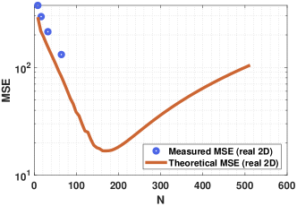
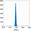
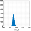
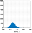
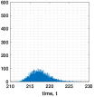
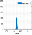
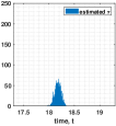
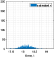
The top row of Fig. 8 shows the estimated depth map at four different resolutions. The estimation is done using the ML estimation. The bottom row of Fig. 8 shows the distribution of the ML estimates. This distribution is obtained through a bootstrap procedure where we sample with replacement time stamps to estimate the time, and we bootstrap for times. The shrinking variance confirms that as we use fewer pixels, the estimation quality improves. The right hand side of Fig. 8 shows the theoretically predicted MSE and the measured MSE. The measured MSE is obtained by first constructing a pseudo ground truth from all the 10,000 frames (with pre-processing). We draw samples from each pixel, sampled with replacement repeatedly 100 times, to compute the MSE.
The result in Fig. 8 does not show a valley. This is because the optimal , by taking derivative of Eq. 30, is . Therefore, if the pulse width is short so is small, it is possible that the optimal is larger than the physical resolution of the SPAD. In this case, maximizing the resolution is the best option.
5 Conclusion
A closed-form expression of the resolution limit for a SPAD sensor array is presented. It is found that the MSE decreases when the total amount of flux is high, the scene is smooth, and the pulse width is small. The MSE demonstrates a U-shape as a function of the number of pixels in a unit space. When the optimal is beyond the physical resolution of the sensor, no binning would be required. Extension of the theory to pile-up effects and non-Gaussian pulse is achievable with numerical integration. Advanced post-processing can possibly outperform the predicted bound which is based on ML estimation.
Acknowledgement
We thank the anonymous reviewers and the area chair for the meticulous review of this paper and, for offering insightful and constructive feedback. We are particularly thankful to Reviewer SxN3 for trusting us on this revision. We thank Abdullah Al Shabili for the initial investigation of the LiDAR statistics. We thank Jonathan Leach’s lab at Heriot-Watt University, and German Mora-Martin of the University of Edinburgh for collecting and sharing the data with us.
The work is supported, in part, by the DARPA / SRC CogniSense JUMP 2.0 Center, NSF IIS-2133032, and NSF ECCS-2030570.
All plots presented in this paper can be reproduced using the code provided at https://github.itap.purdue.edu/StanleyChanGroup/.
References
- Abshire and McGarry [1987] James B. Abshire and Jan F. McGarry. Estimating the arrival times of photon-limited laser pulses in the presence of shot and speckle noise. J. Opt. Soc. Am. A, 4(6):1080–1088, 1987.
- Altmann et al. [2016] Yoann Altmann, Ximing Ren, Aongus McCarthy, Gerald S. Buller, and Steve McLaughlin. LiDAR waveform-based analysis of depth images constructed using sparse single-photon data. IEEE Transactions on Image Processing, 25(5):1935–1946, 2016.
- Bar-David [1969] Israel Bar-David. Communication under the poisson regime. IEEE Transactions on Information Theory, 15(1):31–37, 1969.
- Boretti [2024] Alberto Boretti. A perspective on single-photon LiDAR systems. Microwave and Optical Technology Letters, 66(1):e33918, 2024.
- Chan [2021] Stanley H. Chan. Introduction to Probability for Data Science. Michigan Publishing, 2021.
- Chimitt et al. [2024] Nicholas Chimitt, Xingguang Zhang, Yiheng Chi, and Stanley H. Chan. Scattering and gathering for spatially varying blurs. IEEE Transactions on Signal Processing, 2024. To appear. Available online at https://arxiv.org/abs/2303.05687.
- Choi et al. [2018] Joon Hee Choi, Omar A. Elgendy, and Stanley H. Chan. Image reconstruction for quanta image sensors using deep neural networks. In 2018 IEEE International Conference on Acoustics, Speech and Signal Processing (ICASSP), pages 6543–6547, 2018.
- Coates [1968] Peter Coates. The correction for photon ‘pile-up’ in the measurement of radiative lifetimes. Journal of Physics E: Scientific Instruments, 1(8):878, 1968.
- Dutton et al. [2016] Neale A. W. Dutton, Istvan Gyongy, Luca Parmesan, Salvatore Gnecchi, Neil Calder, Bruce R. Rae, Sara Pellegrini, Lindsay A. Grant, and Robert K. Henderson. A SPAD-based QVGA image sensor for single-photon counting and quanta imaging. IEEE Transactions on Electron Devices, 63(1):189–196, 2016.
- Elgendy and Chan [2018] Omar A. Elgendy and Stanley H. Chan. Optimal threshold design for quanta image sensor. IEEE Transactions on Computational Imaging, 4(1):99–111, 2018.
- Erkmen and Moision [2009] Baris I. Erkmen and Bruce Moision. Maximum likelihood time-of-arrival estimation of optical pulses via photon-counting photodetectors. In 2009 IEEE International Symposium on Information Theory, pages 1909–1913, 2009.
- Fossum [2023] Eric R. Fossum. The Invention and Development of CMOS Image Sensors, chapter 23, pages 281–291. John Wiley & Sons, Ltd, 2023.
- Fossum et al. [2016] Eric R. Fossum, Jiaju Ma, Saleh Masoodian, Leo Anzagira, and Rachel Zizza. The quanta image sensor: Every photon counts. Sensors, 16(8), 2016.
- Gupta et al. [2019a] Anant Gupta, Atul Ingle, and Mohit Gupta. Asynchronous single-photon 3D imaging. In 2019 IEEE/CVF International Conference on Computer Vision (ICCV), pages 7908–7917, 2019a.
- Gupta et al. [2019b] Anant Gupta, Atul Ingle, Andreas Velten, and Mohit Gupta. Photon-flooded single-photon 3D cameras. In 2019 IEEE/CVF Conference on Computer Vision and Pattern Recognition (CVPR), pages 6763–6772, 2019b.
- Hadfield et al. [2023] Robert H. Hadfield, Jonathan Leach, Fiona Fleming, Douglas J. Paul, Chee Hing Tan, Jo Shien Ng, Robert K. Henderson, and Gerald S. Buller. Single-photon detection for long-range imaging and sensing. Optica, 10(9):1124–1141, 2023.
- Heide et al. [2018] Felix Heide, Steven Diamond, David B. Lindell, and Gordon Wetzstein. Sub-picosecond photon-efficient 3D imaging using single-photon sensors. Scientific Reports, 8(1):17726, 2018.
- Henderson et al. [2019] Robert K. Henderson, Nick Johnston, Francescopaolo Mattioli Della Rocca, Haochang Chen, David Day-Uei Li, Graham Hungerford, Richard Hirsch, David Mcloskey, Philip Yip, and David J. S. Birch. A time correlated SPAD image sensor in 40-nm CMOS technology. IEEE Journal of Solid-State Circuits, 54(7):1907–1916, 2019.
- Kay [2013] Steven Kay. Fundamentals of Statistical Signal Processing: Practical Algorithm Development. Prentice-Hall PTR, 2013.
- Kirmani et al. [2014] Ahmed Kirmani, Dheera Venkatraman, Dongeek Shin, Andrea Colaço, Franco N. C. Wong, Jeffrey H. Shapiro, and Vivek K Goyal. First-photon imaging. Science, 343(6166):58–61, 2014.
- Lee et al. [2023] Jongho Lee, Atul Ingle, Jenu V. Chacko, Kevin W. Eliceiri, and Mohit Gupta. CASPI: collaborative photon processing for active single-photon imaging. Nature Communications, 14(1):3158, 2023.
- Li et al. [2023] Zhaohui Li, Haifeng Pan, Guangyue Shen, Didi Zhai, Weihua Zhang, Lei Yang, and Guang Wu. Single-photon LiDAR for canopy detection with a multi-channel Si SPAD at 1064 nm. Optics & Laser Technology, 157:108749, 2023.
- Lindell et al. [2018] David B. Lindell, Matthew O’Toole, and Gordon Wetzstein. Single-photon 3D imaging with deep sensor fusion. ACM Trans. Graph., 37(4):113.1–113.12, 2018.
- Ma et al. [2020] Sizhuo Ma, Shantanu Gupta, Arin C. Ulku, Claudio Bruschini, Edoardo Charbon, and Mohit Gupta. Quanta burst photography. ACM Trans. Graph., 39(4), 2020.
- McCarthy et al. [2013] Aongus McCarthy, Nils J. Krichel, Nathan R. Gemmell, Ximing Ren, Michael G. Tanner, Sander N. Dorenbos, Val Zwiller, Robert H. Hadfield, and Gerald S. Buller. Kilometer-range, high resolution depth imaging via 1560 nm wavelength single-photon detection. Opt. Express, 21(7):8904–8915, 2013.
- Mora-Martín et al. [2021] Germán Mora-Martín, Alex Turpin, Alice Ruget, Abderrahim Halimi, Robert Henderson, Jonathan Leach, and Istvan Gyongy. High-speed object detection with a single-photon time-of-flight image sensor. Opt. Express, 29(21):33184–33196, 2021.
- Morimoto et al. [2020] Kazuhiro Morimoto, Andrei Ardelean, Ming-Lo Wu, Arin Can Ulku, Ivan Michel Antolovic, Claudio Bruschini, and Edoardo Charbon. Megapixel time-gated SPAD image sensor for 2D and 3D imaging applications. Optica, 7(4):346–354, 2020.
- Pediredla et al. [2018] Adithya K. Pediredla, Aswin C. Sankaranarayanan, Mauro Buttafava, Alberto Tosi, and Ashok Veeraraghavan. Signal processing based pile-up compensation for gated single-photon avalanche diodes. 2018. Available at https://arxiv.org/abs/1806.07437.
- Po et al. [2022] Ryan Po, Adithya Pediredla, and Ioannis Gkioulekas. Adaptive gating for single-photon 3D imaging. In 2022 IEEE/CVF Conference on Computer Vision and Pattern Recognition (CVPR), pages 16333–16342, 2022.
- Poisson et al. [2022] Valentin Poisson, Van Thien Nguyen, William Guicquero, and Gilles Sicard. Luminance-depth reconstruction from compressed time-of-flight histograms. IEEE Transactions on Computational Imaging, 8:148–161, 2022.
- Qian et al. [2024] Xuanyu Qian, Wei Jiang, and M. Jamal Deen. Single photon detectors for automotive LiDAR applications: State-of-the-art and research challenges. IEEE Journal of Selected Topics in Quantum Electronics, 30(1: Single-Photon Technologies and Applications):1–20, 2024.
- Rapp and Goyal [2017] Joshua Rapp and Vivek K Goyal. A few photons among many: Unmixing signal and noise for photon-efficient active imaging. IEEE Transactions on Computational Imaging, 3(3):445–459, 2017.
- Rapp et al. [2020] Joshua Rapp, Julian Tachella, Yoann Altmann, Stephen McLaughlin, and Vivek K Goyal. Advances in single-photon Lidar for autonomous vehicles: Working principles, challenges, and recent advances. IEEE Signal Processing Magazine, 37(4):62–71, 2020.
- Richardson et al. [2009] Justin Richardson, Richard Walker, Lindsay Grant, David Stoppa, Fausto Borghetti, Edoardo Charbon, Marek Gersbach, and Robert K. Henderson. A 32×32 50ps resolution 10 bit time to digital converter array in 130nm CMOS for time correlated imaging. In 2009 IEEE Custom Integrated Circuits Conference, pages 77–80, 2009.
- Scholes et al. [2023] Stirling Scholes, German Mora-Martin, Feng Zhu, Istvan Gyongy, Phil Soan, and Jonathan Leach. Fundamental limits to depth imaging with single-photon detector array sensors. Nature Scientific Reports, 13(1):176, 2023.
- Shin et al. [2013] Dongeek Shin, Ahmed Kirmani, Vivek K Goyal, and Jeffrey H. Shapiro. Information in a photon: Relating entropy and maximum-likelihood range estimation using single-photon counting detectors. In 2013 IEEE International Conference on Image Processing, pages 83–87, 2013.
- Shin et al. [2015] Dongeek Shin, Ahmed Kirmani, Vivek K Goyal, and Jeffrey H. Shapiro. Photon-efficient computational 3-D and reflectivity imaging with single-photon detectors. IEEE Transactions on Computational Imaging, 1(2):112–125, 2015.
- Snyder and Miller [1991] Donald L. Snyder and Michael I. Miller. Random Point Processes in Time and Space. Springer, 1991.
- Tachella et al. [2019] Julián Tachella, Yoann Altmann, Nicolas Mellado, Aongus McCarthy, Rachael Tobin, Gerald S. Buller, Jean-Yves Tourneret, and Stephen McLaughlin. Real-time 3D reconstruction from single-photon lidar data using plug-and-play point cloud denoisers. Nature Communications, 10(1):4984, 2019.
- Tontini et al. [2024] Alessandro Tontini, Sonia Mazzucchi, Roberto Passerone, Nicolò Broseghini, and Leonardo Gasparini. Histogram-less LiDAR through SPAD response linearization. IEEE Sensors Journal, 24(4):4656–4669, 2024.
- Ulku et al. [2019] Arin Can Ulku, Claudio Bruschini, Ivan Michel Antolović, Yung Kuo, Rinat Ankri, Shimon Weiss, Xavier Michalet, and Edoardo Charbon. A 512 × 512 SPAD image sensor with integrated gating for widefield FLIM. IEEE Journal of Selected Topics in Quantum Electronics, 25(1):1–12, 2019.
- Villa et al. [2021] Federica Villa, Fabio Severini, Francesca Madonini, and Franco Zappa. SPADs and SiPMs arrays for long-range high-speed light detection and ranging LiDAR. Sensors, 21(11), 2021.
- Wayne et al. [2022] Michael Wayne, Arin Ulku, Andrei Ardelean, Paul Mos, Claudio Bruschini, and Edoardo Charbon. A 500 × 500 dual-gate SPAD imager with 100 IEEE Transactions on Electron Devices, 69(6):2865–2872, 2022.
- Wei et al. [2023] Mian Wei, Sotiris Nousias, Rahul Gulve, David B. Lindell, and Kiriakos N. Kutulakos. Passive ultra-wideband single-photon imaging. In Proceedings of the IEEE/CVF International Conference on Computer Vision (ICCV), pages 8135–8146, 2023.
- Xin et al. [2019] Shumian Xin, Sotiris Nousias, Kiriakos N. Kutulakos, Aswin C. Sankaranarayanan, Srinivasa G. Narasimhan, and Ioannis Gkioulekas. A theory of fermat paths for non-line-of-sight shape reconstruction. In 2019 IEEE/CVF Conference on Computer Vision and Pattern Recognition (CVPR), pages 6793–6802, 2019.
- Yang et al. [2012] Feng Yang, Yue M. Lu, Luciano Sbaiz, and Martin Vetterli. Bits from photons: Oversampled image acquisition using binary poisson statistics. IEEE Transactions on Image Processing, 21(4):1421–1436, 2012.
Supplementary Material
6 Proof of Theorems
In this section, we present the proofs of the theorems. To clarify the contributions of this paper, we add comments to each proof to highlight whether this is based on existing theory or it is a new proof.
6.1 Axioms
We first state the three axioms for inhomogeneous Poisson processes [38].
6.2 Proof of Theorem 1
Remark: This proof is adopted from Bar-David [3] with new elaborations provided for each step.
Consider a set of time stamps . For each timestamp , we consider an infinitesimal width . The probability that one and only one photon falls in each of the intervals and none outside is
As , the intervals merge to become . Therefore,
Regrouping the terms, we can show that
6.3 Proof of Theorem 2
Remark: This proof is adopted from Bar-David [3].
Let’s assume that is a twice differentiable function. Then, let , and decompose as , where is a zero-mean random variable. Similarly, decompose as . Then,
6.4 Proof of Theorem 3
Remark: This is a new proof we make for this paper.
We consider . Using Approximation 1, we write
By Approximation 3, we can show that
where is based on a simple switch between the roles of and in a Gaussian distribution, and is based on the fact that the convolution of two Gaussian probability density functions is equivalent to adding two Gaussian random variables.
If we restrict ourselves to , then we will obtain . Therefore, using the fact that since integrates to 1, we can show that
6.5 Proof of Theorem 4
In proving Theorem 4, we need a few lemmas. The first lemma is the classical bias-variance trade-off.
Remark: The decomposition of the MSE into bias and variance can be found in most of the machine learning textbooks. For completeness and in the context of our paper, we provide the derivations here.
The second expectation in the above is zero because for every according to Lemma 7.
Remark: This is a new proof we make for this paper.
Proof of Lemma 3
Integrating over the unit space , we can show that
Let’s calculate the individual error . Let be the mid-point of and . That is,
Then, we can take the first order approximation of around :
Since by construction, it follows that
Summing over all ’s will give us
where .
Remark: This is a new proof we make for this paper.
Proof of Lemma 4.
Firstly, we use Theorem 3 and apply it to the single-pixel case in Theorem 2. Then, under the assumption that , we can follow Example 3 to show that
Therefore, for a unit length, it follows that
| var | |||
7 Proof of Additional Results
7.1 Proof of Corollary 1
Remark: This proof is adopted from [3].
The probability of observing occurrence is
The integration limit comes from the fact that the time stamps follow the order . The integral is equivalent to of the hypercube . Thus,
7.2 Proof of Corollary 2
Remark: Bar-David hinted the result in [3], but the proof was missing. We provide the proof here.
The sum of the integrals can be written as follows.
Since is an ordered sequence of time stamps, we can rewrite the integration limits by taking into consideration the combinations of the orders. This will give us
7.3 Proof of Lemma 1
Remark: This is a new proof we make for this paper
The KL-divergence of the two distributions is
Taking the derivative with respect to will yield
Equating this to zero and rearranging terms will give us
| (36) |
7.4 Cramer Rao Lower Bound
Remark: The Cramer-Rao lower bound for single-photon LiDAR has been previously mentioned in [36]. We provide the proof here for completion.
Proof of Corollary 3.
Let . Then
Taking the expectation over , we have
Without loss of generality, we set . Taking the reciprocal completes the proof.
8 Auxiliary Results and Proofs
In this section, we present additional results and proofs that are essential to the development of our theories.
8.1 Lemma about Product of Functions
Remark: This proof is adopted from Bar-David.
Proof of Lemma 5.
The expectation can be shown as follows.
Substituting the definition of into the expression above, we can show that
where is defined as .
Now, consider a slightly different integration
where . The difference between this integral and the previous integral is that the previous integral is based . To account for the shape from this triangle to the full hypercube, we add the factors. This will give us
Therefore,
8.2 Lemma about Characteristic Function
Remark: Bar-David mentioned the idea but we could not find the proof. Therefore, the proof here is new.
Proof of Lemma 6.
For the defined, we can show that
If we restrict , then .Therefore,
where the last equality holds whenever is a symmetric function.
8.3 Lemma for and
Remark: Similar to the previous Lemma, Bar-David mentioned the idea but we could not find the proof. Therefore, the proof here is new.
Proof of Lemma 7.
Let the characteristic function of the random variable be
| (40) |
For , we can show that
Since the width of the pulse is much smaller than the interval , we can make without loss of generality.
8.4 Lemma for and
Remark: Similar to the previous Lemma, Bar-David mentioned the idea but we could not find the proof. Therefore, the proof here is new.
Proof of Lemma 8.
The characteristic function of is
| (41) |
Similar to Lemma 7, we define
| (42) |
Then, the function , where , and its derivatives are
With some simplifications, we can show that
Therefore,
Similarly, we can show that
Subtracting the mean square will give us
9 Detailed Setups of Experiments
For the experiments we presented in the main text, the parameters are configured as Table 1. The parameters here are unit-free in the sense they are picked to elaborate the theory.
| number of pixels | ||
| spatial coordinate | ||
| temporal duration | ||
| width of each pixel | ||
| spatial grid spacing | 1/2048 | |
| temporal grid spacing | 1/256 | |
| pulse width | 0.5 | |
| overall scene flux | 10000 | |
| noise floor | 0 | |
| spatial Gaussian radius | ||
| th pixel of | use gradient |
9.1 Ground Truth Time-of-Arrival Function
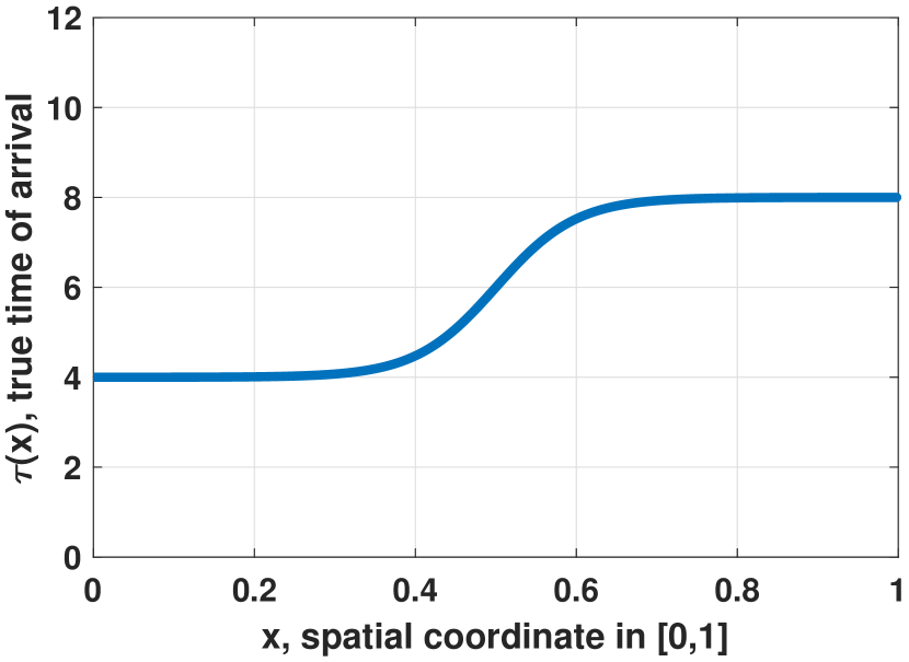
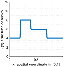
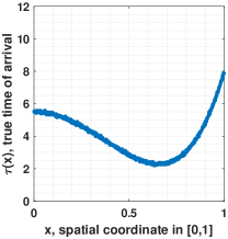
The true time of arrival function can be any function defined on . For example, in the main text, we consider a two-step scene with a smooth transition. Therefore, we can pick a sigmoid function of the following form.
| (43) |
The shape for this particular model is shown in Fig. 11 below. We stress that this is just one of the many models we can pick.
To compute the gradient , the computationally efficient way is to perform finite difference instead of the analytic form. In MATLAB, this can be done using the command gradient.
The division by dx at the end is a reflection of the finite difference operation. For example, at , the true gradient is
Since finite difference gradient only computes , we need to divide the result by to compensate for the spatial interval.
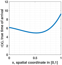
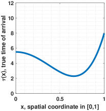
9.2 What if we use a different ?
A critical observation of our theory is that the MSE can be decomposed into bias and variance. The variance has some subtle but important dependency on the shape of , but the bias term will experience more impact.
According to Lemma 3, the bias can be approximated by
| (44) |
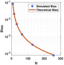
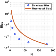
where , with being the gradient of . Therefore, as changes, will change accordingly. Figure 12 illustrates two examples. In the same figure, we also plot the theoretically predicted bias and the simulated result. When is relatively smooth, the theory has an excellent match with the simulation.
 |
 |
 |
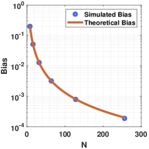 |
Limitations. With no surprise, the piecewise constant approximation has limitations. (1) When the function is intrinsically discontinuous, the theory will not be able to keep track of the trend. (2) When the function is noisy, then the gradient will be overestimated. Both will lead to degradation of the bias estimation, as illustrated in Fig. 13.
 |
 |
 |
 |
Not all limitations can be analytically mitigated. For example, mitigating the discontinuity requires us to know the location of the discontinuous points. In practice, the likely solution is to numerically integrate the error. However, we will not be able to retain a clean, interpretable, and elegant formula.
For the noise problem, we can model the true time of arrival function as
where is a random process denoting the noise, e.g., . In this case, the bias will become
With some calculations, we can show that
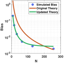
where , with being the slope of the clean signal . Therefore, if we are given the noisy time of arrival , we first need to recover the clean so that we can estimate the correct . Then, the noise variance is added to compensate for the noise term. The correction can be visualized in Fig. 14.
 |
 |
10 Unit Conversion
For our theoretical analysis to match a realistic sensor, a conversion between the size of a physical pixel and the size of a point in the numerical grid needs to be established. In what follows, we present a specific example with some specific numbers. These can be easily translated to other configurations.
Suppose that the overall size of the SPAD array is 10mm as shown in Fig. 15 below. This 10mm would correspond to 1 unit space. Suppose that we use 1024 points in the numerical grid to measure the array. Then, the width of each pixel is
For this paper’s analysis, let’s assume that we group 32 points (for example) as one super-pixel. The width of each super-pixel is therefore
Now, if we want to use a Gaussian to approximate the boxcar kernel, then the standard deviation of the Gaussian should be
For the temporal axis, we take a similar approach. Suppose that the total duration of the measurement is 100ns, and we use 2048 time points to measure the total duration. Then, each time point would correspond to
A typical pulse has a width of around 2ns-6ns. So, suppose that we define the pulse standard deviation as time points, then
Since of a Gaussian can capture 99% of the energy, we can safely say that the width of the pulse is around
which is reasonably inside the 2ns-6ns range.
11 Sampling Procedure
In the main text, we outlined a procedure to generate time stamps according to a Gaussian pulse. This section discusses how to extend the idea to arbitrary pulse shapes.
11.1 Inverse CDF Method
When the pulse has a completely arbitrary shape and when the noise floor is not a constant, we will not be able to draw samples from distributions with known formulae. In this case, the sampling can be done using the inverse cumulative distribution function (inverse CDF) technique [5, Ch.4.9].
The concept of sampling from a known PDF is to leverage the cumulative distribution function (CDF) and a uniform random variable. A classical result shows the following. Suppose that there is a random variable generated from a distribution with a CDF . If , and if we send to the inverse CDF , then the transformed random variable will follow the distribution .
The specific steps to perform the inverse CDF are as follows.
-
•
Step 1: Compute the CDF . Assuming that is invertible, compute the inverse mapping . To obtain for a given , we numerically build a lookup table.
-
•
Step 2: Compute the number of samples . Then, generate random samples by sending uniform random variables: , where , and . Then will follow the probability distribution .
11.2 Implementation and Demonstration
In terms of implementation, we can use the following MATLAB code. Suppose that we are given the received pulse . Then, we can integrate to obtain the CDF . On a computer, the command cumsum will serve the purpose of generating the CDF. Once the CDF is numerically determined, we send uniform random variables to . The inversion is performed numerically by finding the closest such that can give , where is the uniform random variable.
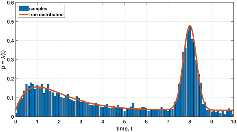
Fig. 16 shows a demonstration where we generate time stamps. The underlying pulse shape is Gaussian, but we also assume a nonlinear noise floor. Specifically, the noise floor mimics a scattering medium which is modeled by a Gamma distribution.
 |
 |
12 Non-zero Noise Floor
The goal of the main text is to derive a simple and informative MSE equation. This is achieved by assuming that the pulse is Gaussian and there is no noise. In this section, we discuss how the theoretical results can be derived for arbitrary pulses, by means of a numerical scheme.
12.1 Maximum Likelihood Estimation
Assuming that the transmitted pulse is and the received pulse is . Here, we assume that can take an arbitrary shape and . We also assume that there is a spatial kernel which will be applied to to yield the resulting space-time function :
The convolution can be implemented numerically. In MATLAB, we can use the command imfilter:
Following the same derivations as the main text, we let be the mid point of each spatial interval and define the effective pulse as
where we emphasize that has an underlying parameter which needs to be estimated. Then, the time of arrivals will follow the distribution specified by the effective return pulse .
The questions we need to ask now are (1). how to estimate the time of arrival , (2). what is the variance ?
For the purpose of deriving theoretical bounds, the estimator we use is the maximum likelihood estimator. The ML estimator is the one that maximizes the likelihood function. In our case, it is
| (45) |
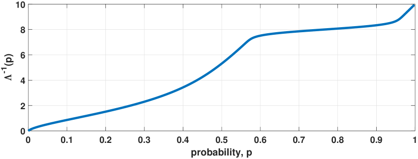
The shape of the likelihood function as a function of the parameter is shown in Fig. 17, for a typical Gaussian pulse with a non-zero noise floor. The likelihood function has a clear maximum (minimum if we take the negative log likelihood) around the true parameter. For the specific example shown in Fig. 17, we use the following configurations: , , where and . We randomly generate random vectors for . We plot the negative log-likelihood as a function of the parameter . The negative log-likelihood functions are random because are random. We take the expectation of these random negative log-likelihood functions to visualize the mean function.
An equivalent alternative approach is to perform the estimation by solving a zero-finding problem. Taking the derivative of with respect to , we can show that the solution must satisfy the equation
| (46) |
Then, the maximum likelihood estimate is determined by finding the zero-crossing of the derivative such that .
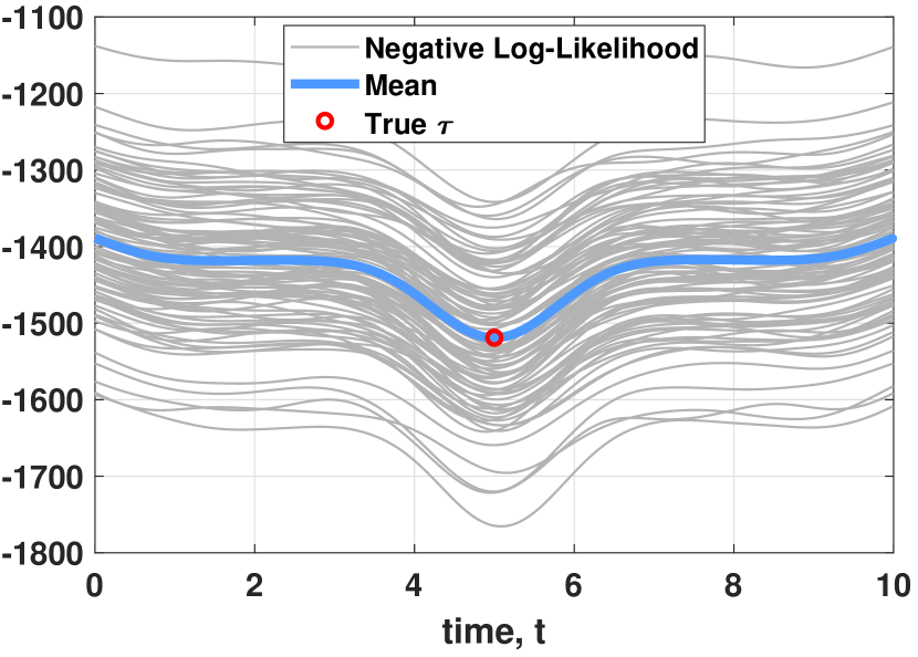
The shape of the likelihood derivative can be seen in Fig. 18, for a typical example outlined in the description of Fig. 17. The maximum likelihood estimate is the zero-crossing of the derivative. We emphasize that for arbitrary pulse shape and a non-zero floor noise, neither the zero-finding approach nor the matched filter approach would have an analytic solution. We will discuss the numerical implementation shortly.
12.2 MSE Calculation
Given the effective return pulse , the MSE follows from Theorem 2. To make our notations consistent, we assume that takes the form
| (47) |
for some function . This assumption is valid whenever and are independent of so that any spatial convolution applied to construct will not affect . Under this notation, we follow Theorem 2 and write the variance of the estimator
| (48) |
where is the derivative of with respect to .
For arbitrary pulse shape, does not have any analytic expression, so does . Nevertheless, the integration in Eq. 49 can still be performed numerically. The MATLAB code below shows how we can do it numerically.
With Eq. 48 defined, the overall MSE as a function of the number of pixels is as follows.
Here, we use the fact that has the same value for all so it does not matter which we use to calculate the variance. Although Eq. 49 is no longer a closed-form expression, it still preserves the shape of the resolution limit where the MSE decays quadratically with respect to and increases linearly with respect to .
12.3 Solving the ML Estimation
In this subsection, we explain how to implement the maximum likelihood estimation for an arbitrary pulse and noise floor. There are three ways to do this.
Approach 1: Gradient-based Likelihood Maximization. For pulses with a known analytic expression, the most straightforward approach is to perform gradient descent with the gradient :
for some step size . Most numerical software such as MATLAB has built-in optimization packages to accomplish this step. For example, using fminunc, we will be able to find the maximum of the likelihood function.
The example below assumes a Gaussian pulse so that we have a closed-form expression for the likelihood function.
To solve the actual maximization we do
where tau0 is the initial guess. For the purpose of deriving the “oracle” maximum likelihood estimate (so that we are not penalized by having a bad algorithm), we use the ground truth as the initial guess. Readers may worry that this would return us the ground truth as the maximum likelihood estimate, i.e., . We note that this will never happen because the likelihood needs to fit the measured time stamps and so is a random function. Since is a random function, the maximum location is a random variable too. Therefore, while the expected value of the estimate is the true , for a particular realization will never be the same as .
Approach 2: Search-based Likelihood Maximization. For arbitrary pulse shape, the gradient-based approach is difficult to implement because the pulse is numerically a different function when we use a different . The viable approach, as we mentioned in the previous subsection, is to run a matched filter. A matched filter requires us to shift the known pulse to the left or to the right until we see the best fit to the data. On computers, we need to perform two steps:
-
•
Given a current estimate and a perturbation , translate it to the time index of the numerical array .
-
•
Shift the index based on the amount corresponding to , and calculate .
In MATLAB, the shifting operation can be implemented using the commands below.
The padding is a band-aid for a MATLAB specific command circshift which circularly shifts the indices. If we do not pad the array appropriately, a pulse located near the end of the time axis will cause erroneous values to the likelihood function after they get circularly flipped to the beginning of time.
Because of the shifting operations defined above, the function call is significantly harder for automatic differentiation unless we customize the step size. The reason is that if the default step size is smaller than the temporal grid we used to define the pulse, two adjacent indices will remain the same. Thus the gradient will be zero. A workaround solution is to go with a non-gradient optimization. For MATLAB, we can use the package fminsearch.
Approach 3: Zero-finding of the Likelihood Gradient. The third approach we can use is to directly solve for the maximum likelihood solution. Recall from Eq. 46 that the maximum likelihood estimate must be the zero-crossing point of Eq. 46, we can directly implement the derivative as a function call such as the example below.
Then, we can use fzero to find the zero-crossing point.
Which approach is faster? Since the goal of this paper is not to provide an algorithm, we skip a formal complexity analysis of the methods. To give readers a rough idea of the comparison between the three approaches, on a typical experiment using the same machine, the runtime is as follows.
| Method | Command | Runtime | |
|---|---|---|---|
| 1 | Gradient descent | fminunc | 0.064 sec |
| 2 | Matched filter | fminsearch | 0.034 sec |
| 3 | Zero crossing | fzero | 0.016 sec |
We remark that all three methods give nearly identical solutions up to the precision of the numerical grid we set.
12.4 Experimental Results
To convince readers that Eq. 49 can be numerically implemented and matches with simulation, we show in Fig. 19 the comparison between the simulation and the theoretical prediction for a range of values. As is evident from the plot, the theoretical prediction matches very well with the simulation.
As we have demonstrated in this example, it is sometimes possible to numerically compute the bias and variance so that the theory will match with the simulation. However, by doing so, we will no longer be able to write down the resolution limit in a simple and interpretable closed-form expression. This is not a deficiency of our theory, it is just a sacrifice of clarity and interpretability in exchange for better theoretical precision.
13 Pile-up Effects
Pile up effects refer to the situation where the photo detector responds earlier than the actual arrival of the pulse signal, typically due to the presence of a strong background.
13.1 Distribution
For simplicity, we model the pile up effect as an exponentially decaying distribution in the background, that is,
| (50) |
where is an exponential function parameterized by the reflected laser event rate , and the background event rate [40]. In this case, the sampling of the time stamps will follow from three steps:
-
•
Draw samples. The distribution of these samples is the shape of the pulse . The parameter specifies the average number of incident signal photons.
-
•
Draw samples. These samples follow the distribution (whose mean is ). The parameter specifies the average number of pile-up photons (coming from the background).
-
•
Draw samples, assuming that . These samples follow the distribution .
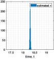
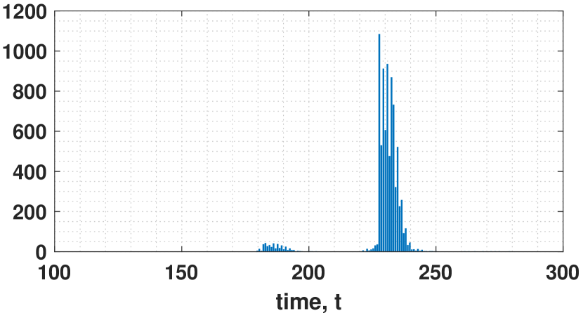
An example of the time stamp histogram is shown in Fig. 20.
13.2 MLE
The maximum likelihood estimation in the presence of the pile up effect needs a separation of background and signal. Because of the simplified model we choose (for the purpose of theoretical illustration), we can exploit the oracle knowledge we know about the pile up and background. Given , we know that the binning is such that
Where we approximate the integral by a simplified function delayed by a time constant .
Given this decomposition of as the signal and the noise part , we use Theorem 2 to estimate the variance of the th pixel:
This integration needs to be evaluated numerically.
In terms of simulation, we need to run the ML estimation. The ML estimation requires us to search for an optimal such that the candidate distribution matches with the measurement. To this end, we follow the procedure outlined in Sec. 12.3 to numerically run a search scheme to pick up the ML estimate.
13.3 Theoretical MSE
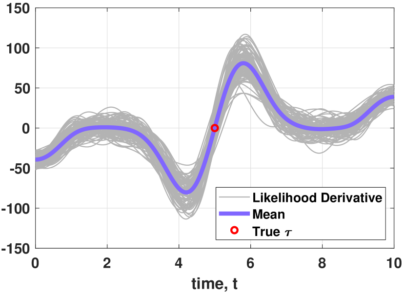
A comparison between the simulated MSE and the theoretically predicted MSE is shown in Fig. 21. For this particular example, we set , , and . The pile up distribution has a constant . Again, we emphasize that these units are unit-free, in the sense they are chosen to illustrate the validity of the theorem rather than matching any particular real sensor.
As we can see in Fig. 21, the theoretical prediction matches extremely well with the simulated MSE. The small deviation towards a larger is due to the fact that the ML estimation faces difficulty when the total number of samples is few. As an example, when , the number of samples per pixel is around 400 whereas when , the number of pixels is around 28,000. When there is no pile up noise, the variance of ML estimate is basically limited by the number of samples. But in the presence of complicated noise (such as pile up), the ML estimation procedure has limitations where it cannot differentiate signal from noise. Therefore, when the number of samples is few, the simulation performance will be worse than what the theory predicts. Nevertheless, Fig. 21 still shows a high degree of match between the theory and the simulation.
14 Dark Count
The model we presented in the main text does not consider dark count. In this section, we briefly discuss how it can be included.
Dark count is a type of sensor noise caused by the random generation of electrons in the depletion region. These random electrons are present even when there is no photoelectric event. Therefore, one way to model dark count is to treat it as a uniform noise floor that does not change over time and does not depend on the scene flux. However, dark counts scale with the sensing area. So, if there are pixels and if we assume that the sensing area scales linearly with , then the dark counts will be reduced by times on average. Therefore, a simple model in the context of this paper is to write
| (51) |
Because of this simple addition to the background, we can treat as part of the background noise. In a typical scenario when the dark count rate is in the order 10 per second while a SPAD can count up to 1 million photons per second (e.g., ThorLab’s single-photon detectors), the impact of dark current is not visible unless we operate it in extremely low-light.
15 Extension to 2D
In this section, we briefly summarize how the results can be extended to 2D. We will derive the bias and the variance.
15.1 Bias
For the bias term, in 2D, we need to consider a 2D coordinate . The time of arrival function is denoted as . The average function is
Where is the th value defined as
The derivative of the time of arrival function, in the 2D case, will become the gradient. This means that
For notational simplicity, we write . If we are interested in the gradient of the th pixel, we write
The magnitude square of the gradient is denoted as , and the overall gradient summed over all the pixels is
where the last approximation holds by assuming that covers the unit squares.
The main result for the bias term in the 2D case is summarized in the lemma below.
Proof of Lemma 9.
We start with the definition of the bias:
Let be the mid-point such that
We can approximate the first order approximation to :
where is the gradient. Then, the error is
Assuming , the above is simplified to
Summing over all ’s will give us
| Bias | |||
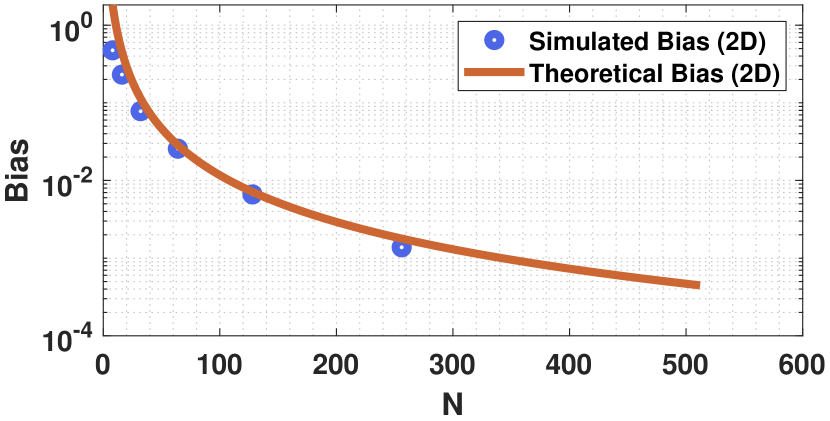
Visualization of the Bias. A visualization of the bias can be seen in Fig. 22. In this example, we use a real depth map as the ground truth . We scale the depth map so that the maximum value is 20, and the minimum value is 10. The full resolution is . To reduce the discontinuity of the depth map at object boundaries, we apply a spatial lowpass filter to smooth out the edges. The estimated gradient magnitude is . We consider four different resolutions , , , and . For each resolution, we use the equation outlined in Lemma 9 to calculate the theoretically predicted bias. We compare this predicted bias with the simulation. As we can see from Fig. 22, the theoretical prediction offers an excellent match with the simulation.
 |
 |
 |
 |
15.2 Variance
For the variance term, we note that the derivation follows similarly to the 1D case:
| Var | |||
Therefore, as long as we can calculate , we will be able to determine the variance.
Based on the arguments we described before stating the lemma, we shall focus on deriving the variance for each individual pixel. To this end, we need to derive the effective return pulse . Following the steps of the proof of Theorem 3, the critical step is the convolution of a 2D spatial Gaussian and a 1D temporal Gaussian
| 2D spatial Gaussian | |||
| 1D temporal Gaussian |
Here, is the spatial radius of the 2D Gaussian, which serves the same role as in the 1D case. The linear approximation is the 2D version of the 1D linear approximation , where is the center pixel in each interval of the grid, and is the gradient at .
Before we proceed to the proof, we state the main result.
Proof of Lemma 10. The core derivation is the convolution between the 2D Gaussian in space and the 1D Gaussian in time. By separability of a 2D Gaussian, we can write the 2D Gaussian as the convolution of two orthogonal 1D Gaussian functions:
The order of versus does not matter. Then, substituting it into the main convolution, we can perform two consecutive convolutions:
The first convolution, following the derivation of Theorem 3, will give us
where is the horizontal component of the gradient .
The second convolution, which is applied after the first convolution, will give us
Restricting ourselves to , we can show that the effective return pulse is
Finally, we recognize that since there are pixels in the unit space, (and assuming that for simplicity), then each pixel will see a total flux of . Therefore,
Summing over and will give us
| Var | |||
Visualizing the Variance. Fig. 23 shows the visualization of the variance as a function of . The experimental configuration is identical to the one we used in the 2D bias analysis. For the purpose of analyzing the variance, we need to further set up a Monte Carlo simulation. To this end, we first set the spatial spacing of the grid as along each direction. The total amount of flux is set as . Suppose that we have pixels on each side, the unit square will have pixels. Each pixel will therefore observe amount of flux. When , the per pixel flux is 15625 photons per pixel. When , the per pixel flux is 15.26 photons per pixel.
For simplicity, we assume that the pulse is Gaussian. The width of the pulse is 2 arbitrary units, which is roughly 10 percent of the true depth value. We also assume that the noise floor is . These two assumptions allow us to use a simple ensemble average as the maximum likelihood estimator. Otherwise, we need to numerically implement the matched filter.
In this particular experiment, we use as the spatial radius, and . The variance is calculated for each pixel and then summed over the entire unit square. A total number of 1000 random trials are conducted to obtain the variance per pixel (and for the whole image).
 |
 |
 |
 |
16 Real 2D Experiment
In this section, we provide additional detail on how real 2D experiments are conducted.
16.1 Snapshot of Real Data
As depicted in the main text, the real data is collected by a SPAD array previously reported by Henderson et al. [18]. The system has a time-to-digital converter (TDC) timing resolution of 35 ps. For convenience, we crop the center region for analysis. Fig. 24 shows a one-frame snapshot of the real data, and the 10,000-frame average. We observe that the 10,000-frame average is noisy, although the shape of the object is visible.
 |
 |
| 1 frame | average of 10,000 frames |
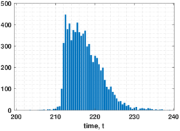
Inspecting the source of the noise, we plot the histogram of one of the pixels of the data volume in Fig. 25. We recognize two issues in the data: (i) There is a secondary pulse, likely caused by secondary bounces from the background; (ii) there is a strong peak happening at the beginning (and sometimes at the end) of the sensing period, likely caused by failed detections of the SPAD. We did not show these samples in the histogram because it is just a strong spike in the histogram. The presence of these two issues makes the average of the time stamps problematic, hence generating noise.
16.2 Pseudo Ground Truth
For the purpose of MSE analysis, we need to construct a pseudo ground truth — a ground truth signal generated from all the available samples, hoping as noise free as possible. To achieve this goal, we need to reject the outliers so that we can retain only the primary pulse.
Our pre-processing step is done by identifying the center of the primary pulse. Once the center is identified, we crop around the center histogram with where is the standard deviation of the pulse.
Two remarks are worth mentioning: (i) The identification of the center of the primary pulse involves a few steps. The first step is to find a coarse estimate of the center. For this purpose, we compute the mean of the entire 10,000 data points and crop a large temporal window around the mean. We smooth out the histogram so that we can pick a more reliable peak. The smoothing step is done by adding Gaussian random variables. (ii) Once the peak is identified, we move to the second stage by putting a small temporal window around the peak. We reject all samples that fall outside this small temporal window, thus effectively removing the secondary pulse and the spike in the beginning and at the end.
After we have cleaned up the data, we can plot the resulting histogram as shown in Fig. 26. The pulse is significantly more concentrated around the true peak. The resulting depth map is slightly over-smoothed. However, since all our subsequent analysis is done based on the processed histogram (as we will be re-sampling with replacement from the processed histogram), computing the MSE with respect to this smoothed depth map will not cause issues to the analysis.
 |
 |
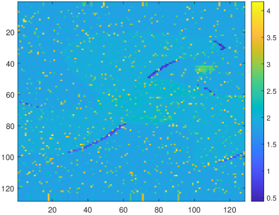
16.3 Estimating and
In the theoretical analysis of the variance, we need to know the pulse width and the total amount of flux .
For , we use the histogram shown in Fig. 26 to compute the variance at every pixel location. Although the pulse is asymmetric, we treat it as a symmetric pulse and compute the standard deviation regardless. We repeat the process for every pixel, and we generate a map of as shown in Fig. 27. For simplicity, we use the average of the in this map as the true value for our theoretical analysis. Our estimated is .
 |
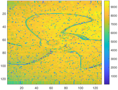 |
For , we again use the histogram shown in Fig. 26 to count the number of elements in the histogram. Recall that during the pre-processing stage, we have already eliminated all the outliers from the raw data. This will leave us with a smaller set of samples compared to the original data array. The number of active samples will inform us about the number of photons arriving at the sensor. During our analysis, we will sample with replacement from the histogram. For each trial, we draw samples from the available data points per pixel. Therefore, the total flux we have in the data is the sum of the values in Fig. 27, divided by 10,000 because we have 10,000 frames, and multiplied by . Approximately our is .
16.4 Variance Estimation via Bootstrap
The main tool we use to evaluate the variance is bootstrap. The idea is that given a dataset of data points, we sample with replacement samples and calculate the estimate of interest. The variance of the estimate is called the bootstrapped variance. When we repeat the random trials for long enough, the bootstrapped variance will converge to the true variance in probability.
Following this idea, for every pixel, we sample with replacement times to generate the samples. From these samples, we construct the ML estimate (for every pixel) where the ML estimation is done by taking the simple average of the samples. Here, we assume that the pulse is symmetric even though it is not. We find that this approximation does not cause too many issues. Once the ML estimate is obtained, we repeat the process times to evaluate the variance.
For lower resolutions, we bin the samples to form a bigger pool. If we use a bin, then the total number of samples to be generated for the bootstrap purpose is samples; If we use a bin, then the total number of samples is samples. These samples will give us an estimate of the real variance of the data.
The theoretical formula of the variance is based on a simpler form . We omitted the because is small compared to . (Recall that ).
16.5 Bias Estimation via Numerical Integration
The bias is computed numerically via integration. The reason is that the pseudo ground truth depth map is overall a piecewise constant function. As we explained in the limitation subsection of the Bias section, there is no simple analytic formula for calculating the bias for piecewise constant functions unless we perform the numerical integration. The numerical integration is done by downsampling and upsampling the cleaned raw data volume. For example, to calculate the bias caused by a bin, we take the average over all the available samples in the (where is the number of available samples). After binning, we scale it back to the full resolution and compute the sum squared error with respect to the pseudo ground truth.
17 Q&A
In this section, we list a few questions and answers which might be of interest to readers.
Q1. Can you just use as many pixels as possible during acquisition, and then perform binning (of the time stamps) as post-processing?
Answer: Yes, this is completely possible. In fact, in our real data analysis, we see that when the pulse is short enough, the MSE decays monotonically with the . Theoretically, the optimal still exists but this could be larger than what the physical resolution of the sensor can support. In this case, we should just maximize the resolution.
From a practical point of view, we also agree that post-processing of noisy time stamps can be cost-effective. Analog processing on the sensor front could also be a solution.
Q2. What if you denoise the estimated time of arrival map? Will it beat your MSE bound?
Answer: Yes, it will. The theory we presented here uses the maximum likelihood (ML) estimation. ML estimation allows us to say things concretely so that we can offer a simple and interpretable MSE estimate. If we do denoising, then we will be doing maximum a posteriori or minimum mean square estimation. In those cases, we need to specify the prior distribution for which no one has a formula. Even if we do pick a prior (e.g., total variation), the derivation of the MSE will be substantially harder if not intractable. So, we lose the capability of writing a simple and interpretable formula. In short, while we are almost certain that a well-defined post-processing will “beat” our MSE bound, this “victory” offers little to no theoretical benefit to the scope of this paper.
Q3. What is the utility of this paper?
Answer: The MSE we show in this paper is, in our honest opinion, simple, interpretable, and elegant. For the first time in the LiDAR literature, we provide the exact characterization of the resolution limit.
Q4. You need to show more comparisons by sending the raw time stamps through a state-of-the-art depth reconstruction neural network.
Answer: Beating a SOTA depth reconstruction neural network is not the purpose of this paper.
Q5. Is MSE the right metric?
Answer: Yes, if you want to derive equations, especially a simple equation to give you intuitions about the problem. No, if you are more interested in practical scenarios. There is no better or worse.
Q6. Your model is inaccurate. It made too many assumptions such as Gaussian pulse, single-bounce, no dark current, constant reflectivity, etc.
Answer: While we also want to be as accurate as possible, accuracy and simplicity are mutually exclusive in this paper. As we have explained in the supplementary material, all these situations can be handled numerically by integrations. But this will defeat the purpose of deriving a closed-form expression.
Q7. Some papers in the literature use the Markov chain/self-excitation process to model the photon arrivals. Why are you skipping all these?
Answer: We are just assuming that there is no dead time. If there is dead time, then you are correct that self-excitation processes are needed to provide a better model. However, this would be substantially more complicated than what we present here. By assuming no dead time, we can go back to the standard inhomogeneous Poisson process by exploiting independence. Even in this significantly simplified case, we see that the derivation of the MSE is non-trivial.
Q8. Can your model handle fog?
Answer: Yes, but it will be complicated. Scattering medium such as fog affects the reflectivity and causes additional background as shown in Figure 16. You will need numerical integration to evaluate the bound.