Using quantum computers in control: interval matrix properties
Abstract
Quantum computing provides a powerful framework for tackling computational problems that are classically intractable. The goal of this paper is to explore the use of quantum computers for solving relevant problems in systems and control theory. In the recent literature, different quantum algorithms have been developed to tackle binary optimization, which plays an important role in various control-theoretic problems. As a prototypical example, we consider the verification of interval matrix properties such as non-singularity and stability on a quantum computer. We present a quantum algorithm solving these problems and we study its performance in simulation. Our results demonstrate that quantum computers provide a promising tool for control whose applicability to further computationally complex problems remains to be explored.
I Introduction
Quantum computing has gained increasing attention in recent years due to its ability to solve certain computationally challenging problems more efficiently than classically possible. This includes, for example, integer factorization [1], unstructured search [2], or linear systems of equations [3], but also the simulation of classical [4, 5] and quantum [6], [7, Section 4.7] systems. However, these algorithms cannot be implemented reliably for relevant problem sizes on current noisy intermediate-scale quantum (NISQ) devices [8] due to problems connected to noise and scalability. Variational quantum algorithms (VQAs) are a promising class of quantum algorithms which combine a quantum computer with a classical optimization algorithm [9]. VQAs involve trainable parameters which are optimized iteratively using, e.g., a gradient descent scheme, and, therefore, they are well-suited for NISQ devices due to their adaptation to small and noisy hardware. The quantum approximate optimization algorithm (QAOA) [10] is one of the most popular VQAs and it can be used to solve a specific class of integer programs: quadratic unconstrained binary optimization (QUBO) problems.
Problems with integer variables are relevant in various domains of systems and control theory and, therefore, QAOA is a promising candidate for achieving computational speedups in control. Further quantum algorithms that can tackle computational control problems are listed in [11]. Yet, the usage of quantum computers in control is largely unexplored, except for results on, e.g., MPC with finite input spaces [12] or decentralized control [13]. In this paper, we propose an algorithm for the verification of interval matrix properties, which is known to be a computationally hard problem, on a quantum computer.
In computational complexity theory, problems can be classified according to the time required for their solution. Problems which can be solved with a polynomial-time algorithm belong to class P and those whose solution can be verified in polynomial time belong to class NP. For NP-hard problems, which are problems to which every problem in NP can be reduced efficiently, there exist no known polynomial-time algorithms on a classical computer. Various control-theoretic problems have been shown to be NP-hard, including static output feedback design or verifying interval matrix properties [14, 15, 16].
In this paper, we introduce an approach for verifying interval matrix properties on a quantum computer. We focus on two main properties: robust non-singularity and robust stability of interval matrices, meaning that all members of the interval matrix are non-singular or stable, respectively. Existing research by [14] shows that the verification of robust non-singularity can be equivalently reformulated as a binary optimization problem. Given that this binary optimization problem is a QUBO problem, it can be tackled using QAOA. The main contribution of this paper is a quantum algorithm based on QAOA which can verify robust non-singularity and robust stability of interval matrices. The applicability is illustrated with numerical examples.
Notation
Let and define the -dimensional discrete cube . For each element , the matrix represents a diagonal matrix with the entries of on its diagonal. Further, for a matrix , we define
| (1) |
The Hermitian conjugate of a matrix is denoted by . Finally, denotes an identity matrix.
II Interval Matrices
In this section, we introduce the concept of interval matrices along with the key properties that are studied in the present paper. An interval matrix is defined as
| (2) |
where and represent an upper and lower bound matrix and the inequality is interpreted element-wise. Further, we define the center of an interval matrix as
| (3) |
This allows to reformulate the lower and upper bound matrices as and with .
II-A Non-singularity of interval matrices
In this paper, we study non-singularity of interval matrices based on the radius of non-singularity. The definition of a non-singular interval matrix is given in the following.
Definition 1.
An interval matrix is non-singular if all matrices are non-singular.
The radius of non-singularity measures the distance of a matrix to the closest singular matrix according to an a priori fixed shifting matrix and is defined as
| (4) | ||||
| s.t. | ||||
This problem minimizes such that the interval matrix is singular, i.e., contains a singular matrix . Given the optimal value of problem (4), a non-singular interval matrix can be defined accordingly as
| (5) |
for any . The radius of non-singularity is relevant, e.g., for sensor processing in the presence of noise [14] or for sensitivity analysis of linear systems [17], and it has close connections to various concepts including the structured singular value which is a powerful tool in robust stability analysis [18]. Further, as we show below, it can be used to study robust stability properties of uncertain linear systems.
As an instructive example, let us consider the matrices
| (6) |
The boundaries of the corresponding interval matrix considered in (4) are given by
| (7) |
The optimal solution of (4) is given by with the associated singular matrix
| (8) |
As shown in [14], the radius of non-singularity of a given, non-singular matrix and a matrix , can be reformulated as a combinatorial optimization problem:
| (9) |
The optimization problem appearing in the denominator is the central problem considered in this paper. The proof of NP-hardness is given in [14] and is sketched briefly in the following. The maximization in (9) can be simplified for the specific choice , which allows to reformulate (9) as
| (10) |
with
| (11) |
II-B Stability of interval matrices
Beyond non-singularity, we also address the problem of stability verification of interval matrices.
Definition 2.
An interval matrix is stable if all matrices are stable, i.e., for all eigenvalues of .
Stability of an interval matrix implies robust stability of the uncertain system
| (12) |
with , which is an important problem in robust control [19]. In [20], it is shown that, just like non-singularity, verifying stability of interval matrices is NP-hard as well. In the following result, we exploit that stability and non-singularity are closely related due to the continuity of eigenvalues in the matrix entries. For simplicity, we focus on symmetric interval matrices. Considering general interval matrices is an interesting issue for future research.
Definition 3.
For an interval matrix , the symmetric interval matrix is defined as
| (13) |
Stability verification of a symmetric interval matrix is relevant in scenarios, where not only uncertainty bounds specified by are available but also additional structural knowledge on symmetry of the dynamics. The following result shows that stability of symmetric interval matrices can be verified based on a non-singularity test.
Proposition 4.
Suppose is a non-singular symmetric interval matrix and there exists a stable . Then, is stable.
Proof. If is stable, then all its eigenvalues have real value less than . Note that all eigenvalues of the matrices in are real due to symmetry. Since eigenvalues are continuous functions in the matrix entries, the non-singularity of implies that all are stable. ∎
Motivated by Proposition 4, we focus on deriving a quantum algorithm for verifying robust non-singularity, which then also allows to verify robust stability of a symmetric interval matrix by testing stability of one of its elements. Note that the eigenvalues of a single matrix can be computed efficiently on a classical computer, which is the only additional step for the stability check.
III Quantum Algorithm
In this section, we propose the quantum algorithm for verifying the interval matrix properties introduced above. First, in Section III-A, we present basic elements of quantum computing that are required to state and implement our algorithm. Next, in Section III-B, the key underlying algorithm QAOA is explained in more detail followed by the construction of the problem Hamiltonian in Section III-C. Finally, the overall algorithm is stated in Section III-D.
III-A Quantum Basics
In the following, we present required basics of quantum computing. For further details, we refer to the tutorial [11], which introduces quantum computing from the perspective of control, as well as to the textbook [7]. Qubits (short for “quantum bits”) are the basic components of a quantum computer, comparable to bits in classical computing. Mathematically, a qubit is written as
| (14) |
for some with . We use the standard Dirac notation for denoting quantum states and for their Hermitian conjugate. The precise value of is not accessible. Instead, a measurement can only reveal that the system is in one of the two basis states
| (15) |
where the probabilities for either outcome are and , respectively. A quantum state consisting of qubits lives in
The second fundamental component of a quantum computer are quantum gates. These are used to manipulate the qubits and they are represented by unitary matrices , i.e., they satisfy . The application of a quantum gate to an input state is defined by multiplication, i.e., the output state is
| (16) |
The Pauli gates , , and are popular examples of quantum gates and they are defined as
| (17) |
For example, applying the gate to a qubit swaps the amplitudes of and as can be seen by
| (18) |
and similarly . The final part of a quantum algorithm is the measurement. In Figure 1, a simple example of a quantum circuit is given which implements the operation (18) with subsequent measurement of the qubit.
& \gateX \meter \rstick
As mentioned above, qubits cannot be measured directly, but a measurement can only return one of a finite number of possible outcomes, where the corresponding probabilities are determined by the probability amplitudes , of the qubit, cf. (14). To be more precise, measurements are always taken w.r.t. an observable . Repeated measurements of a state w.r.t. the observable allow to retrieve the expectation value
| (19) |
For many quantum algorithms, in particular VQAs, this expectation value is the actual output of the algorithm.
III-B Quantum approximate optimization algorithm
VQAs are a class of quantum algorithms combining an optimization procedure on a classical computer with a quantum algorithm [9]. This allows the algorithm to adapt to noise on the quantum computer and, thereby, provide possibly more reliable results. QAOA [10] is an important example of VQAs. It is tailored to solving combinatorial optimization problems and involves alternating between a classical optimization routine to determine parameters of quantum gates and a quantum evolution via the resulting parametrized circuit.
In the following, we provide a brief introduction to QAOA. QAOA can be used to solve problems of the form
| (20) |
for a cost function . The algorithm consists of repeated applications of parametrized unitaries to an initial quantum state . The two unitaries applied to this state are the mixing unitary with mixing Hamiltonian and the problem unitary with problem Hamiltonian . The parameter vectors are optimization variables for the layers of the quantum circuit. These two unitaries are applied to the initial state in an alternating fashion
| (21) |
with . The number of alternations in (21) is problem-specific but typically chosen small to enable implementations on current quantum hardware. Figure 2 shows the -qubit quantum circuit consisting of a measurement of the state
| (22) |
Here, denotes the Hadamard gate defined as
| (23) |
which generates the input state due to
| (24) |
with the Kronecker product .
&\gateH\gate[2]U(β_1,γ_1)\gate[2]U(β_2,γ_2) \meter
\lstick\gateH\meter
Let us now discuss how the mixing and problem Hamiltonians and are chosen. The problem Hamiltonian encodes the cost function into the quantum algorithm, see Section III-C for the construction procedure. On the other hand, the mixing Hamiltonian is used for entangling the solution amplitudes and expanding the solution space to create a diverse set of candidate solutions. The mixing Hamiltonian is commonly chosen independently of the cost function as
| (25) |
where we use the standard notation
| (26) |
Finally, the expectation value
| (27) |
of the parametrized state is determined based on repeated measurements, compare (19). Based on this value, a classical computer determines a new set of parameters and maximizing (27) using some optimization scheme, e.g., gradient descent. This procedure is then repeated until convergence. Figure 3 summarizes the basic scheme of QAOA as an iteration between classical optimization and execution of the quantum algorithm (27).
After converging to a set of parameters , , the candidate solution for (20) is obtained by performing repeated measurements of the resulting quantum state
| (28) | ||||
where we use the standard notation for computational basis states, e.g.,
| (29) |
A measurement of returns the -th computational basis state with probability . The computational basis state with the highest probability (determined empirically by counting occurrences in repeated measurements) is then employed as candidate solution for the original binary optimization problem (20).
III-C Formulating the problem Hamiltonian
In the following, we show how the problem Hamiltonian can be chosen in order to compute the radius of non-singularity via QAOA. Recall the combinatorial optimization problem introduced in (9), i.e.,
| (30) |
In order to apply QAOA, we now transform (30) into a binary optimization problem via a variable transformation from to . More precisely, we introduce the binary variable according to and , resulting in
| (31) |
In order to construct a suitable , the relation
| (32) |
needs to hold for any . Here, is the cost in the new parametrization such that for all and satisfying (31). Indeed, multiplying (32) by from the left-hand side and using unit norm of yields , which is why QAOA aims at maximizing , compare (27).
The following result provides a possible choice of satisfying (32).
Theorem 5.
Proof.
First, (30) is reformulated using that , i.e., . To this end, if is a non-zero, real eigenvalue of , it holds that
| (33) |
Since , it follows that . Together with (33), this implies
| (34) |
Left-multiplying by yields
| (35) |
Subsequently, this results in
| (36) | ||||
The absolute value can be neglected due to the (bi-)linear cost function and the symmetry of . Substituting (31) into , we obtain
| (37) | ||||
with
| (38) | ||||
Note that the Pauli-Z gate satisfies
| (39) |
Applied to (37), this results in
| (40) | ||||
The proof of Theorem 5 consists of two parts: 1) reformulation of the optimization problem (30) as a QUBO and 2) reformulation of the QUBO as a VQA by choosing a suitable problem Hamiltonian . The step 1) is inspired by [14] but faces the additional technical challenge of considering a general rank- matrix rather than . Further, the step 2) follows the derivation in [21], adapted to the specific binary optimization problem considered in the present paper.
III-D The Quantum Algorithm
Algorithm 6 summarizes the overall quantum algorithm verifying robust non-singularity of a given interval matrix . It can also be used to verify stability of a symmetric interval matrix by using Proposition 4.
IV Implementation
In order to examine the performance of the proposed algorithm, we simulate the algorithm using the Pennylane toolbox [22] for Python. The source code for the implementation is publicly accessible on https://github.com/JanKyb/Radius-Of-NonSingularity-using-QAOA.
To verify the performance, we consider two examples. For the first example, the matrices of (6) are reconsidered. Calculating the radius of non-singularity with the proposed quantum algorithm leads to the results in Figure 4. The counts shown in the figure represent an approximation of the probabilities corresponding to the quantum state (28) obtained via the proposed algorithm, followed by an additional conversion step according to (31).
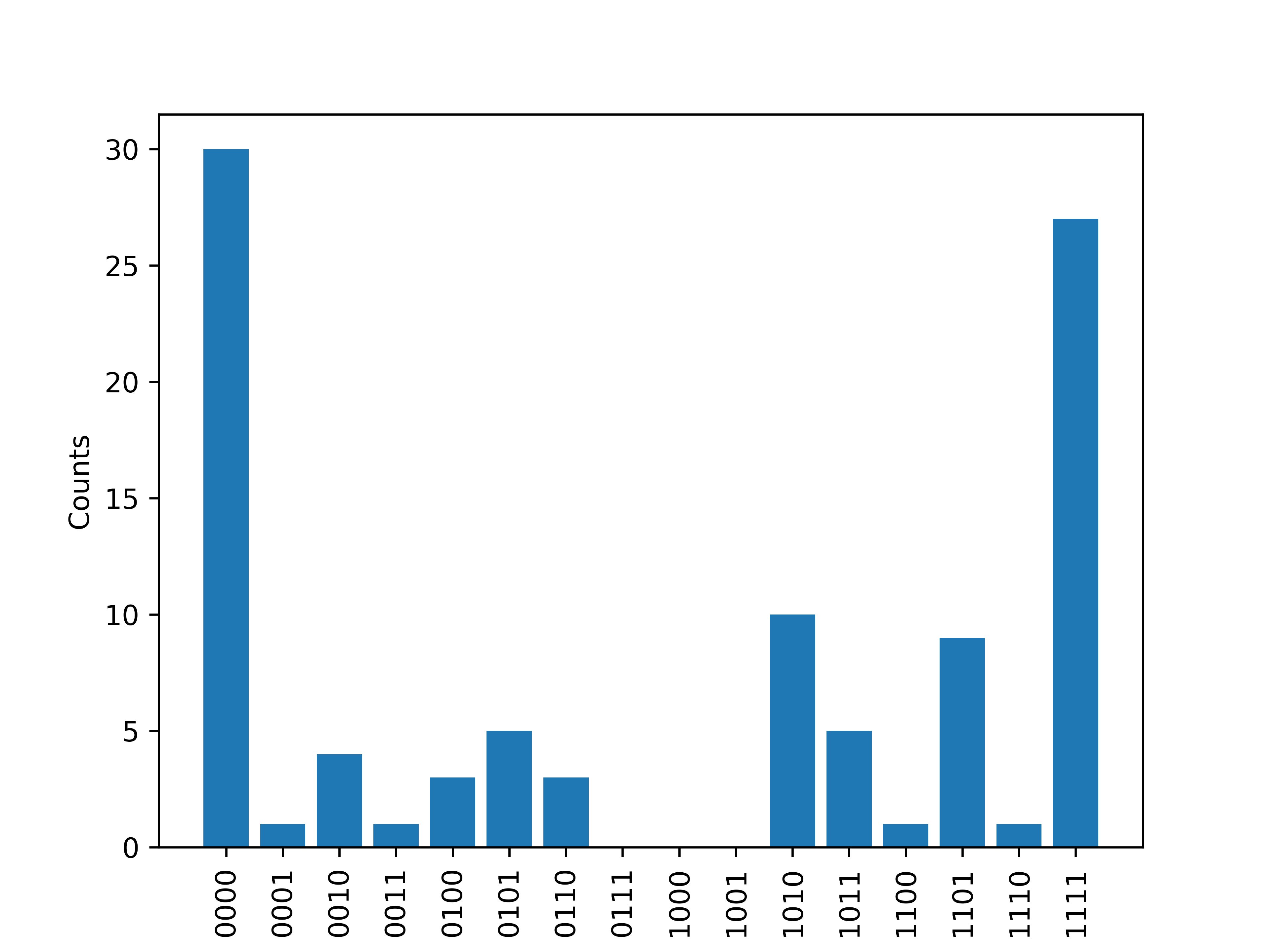
It can be seen, that the first string yields the solution with the (empirically) highest probability, i.e., the maximum amount of counts. Transforming this string back to the initial coordinates based on (31), the corresponding candidate solution of (30) is given by and . This yields the result , which is indeed the correct solution, compare Section II. Note that also the solution string has a comparably large amount of counts. Evaluating the cost function, also yields the same optimal result as , which is due to the symmetry in the variable transformation (31) and the cost function in (30). Moreover, several further strings corresponding to a suboptimal solution also have a non-trivial amount of counts. This characteristic is representative for QAOA being a quantum algorithm with an inherently probabilistic output.
As a second and more realistic example, we study robust stability of an RL circuit from [23], which is a prime example of a symmetric system. The corresponding system matrix is
| (41) |
To analyze robust stability of this system subject to additional uncertainty, we are interested in finding a possibly large value such that all symmetric matrices in are stable, where we consider . In the following, this analysis will be carried out by computing the radius of non-singularity via the proposed quantum algorithm.
An application of Algorithm 6 leads to a distribution of counts analogous to Figure 4. Due to the increased dimension, we do not depict all possible solutions but only list the bit strings with the most counts in Table I.
| binary strings | counts |
|---|---|
The solution with the highest number of counts is . To verify that this is indeed an optimal solution, we use (31) to transform the optimal string into the initial coordinates as and . Plugging this candidate into the cost of (30) yields . Thus, we have and, indeed, is (approximately, i.e., modulo numerical inaccuracies) singular. Using that is stable, Proposition 4 implies that all symmetric matrices in for any are stable.
V Conclusion
Quantum computing is a rapidly advancing technology that promises to solve certain computational problems faster than classically possible. In this paper, we presented a quantum algorithm for verifying non-singularity and stability of interval matrices, which are relevant problems, e.g., in robust stability analysis. The proposed algorithm relies on QAOA which is a popular recent quantum algorithm addressing combinatorial optimization. Extending our results to stability analysis of general (not symmetric) interval matrices as well as the implementation on a real quantum computer are interesting issues for future research. Moreover, given the high relevance of combinatorial optimization problems in various domains of control, applying QAOA to solve computationally complex problems in control poses another promising future research direction. Beyond combinatorial optimization, further computational problems appearing in control may as well be amenable to quantum computing, see [11] for an overview.
References
- [1] P. Shor, “Polynomial-time algorithms for prime factorization and discrete logarithms on a quantum computer,” SIAM Review, vol. 41, no. 2, pp. 303–332, 1999.
- [2] L. K. Grover, “A fast quantum mechanical algorithm for database search,” in Proc. 28th ACM Symposium on the Theory of Computing, 1996, pp. 212–219.
- [3] A. W. Harrow, A. Hassidim, and S. Lloyd, “Quantum algorithm for linear systems of equations,” Physical Review Letters, vol. 103, no. 15, p. 150502, 2009.
- [4] D. Giannakis, A. Ourmazd, P. Pfeffer, J. Schumacher, and J. Slawinska, “Embedding classical dynamics in a quantum computer,” Physical Review A, vol. 105, p. 052404, 2022.
- [5] M. A. Schalkers and M. Möllers, “Efficient and fail-safe collisionless quantum Boltzmann method,” arXiv:2211.14269, 2022.
- [6] R. P. Feynman, “Simulating physics with computers,” Int. J. Theor. Phys., vol. 21, p. 467, 1982.
- [7] M. A. Nielsen and I. L. Chuang, Quantum Computation and Quantum Information: 10th Anniversary Edition, 10th ed. Cambridge University Press, New York, NY, USA, 2011.
- [8] J. Preskill, “Quantum computing in the NISQ era and beyond,” Quantum, vol. 2, p. 79, 2018.
- [9] M. Cerezo, A. Arrasmith, R. Babbush, S. C. Benjamin, S. Endo, K. Fujii, J. R. McClean, K. Mitarai, X. Yuan, L. Cincio, and P. J. Coles, “Variational quantum algorithms,” Nature Reviews Physics, vol. 3, pp. 625–644, 2021.
- [10] E. Farhi, J. Goldstone, and S. Gutmann, “A quantum approximate optimization algorithm,” arXiv:1411.4028, 2014.
- [11] J. Berberich and D. Fink, “Quantum computing through the lens of control: a tutorial introduction,” arXiv:2310.12571, 2023.
- [12] D. Inoue and H. Yoshida, “Model predictive control for finite input systems using the D-wave quantum annealer,” arXiv:2001.01400, 2020.
- [13] S. A. Deshpande and A. A. Kulkarni, “The quantum advantage in decentralized control,” arXiv:2207.12075, 2022.
- [14] S. Poljak and J. Rohn, “Checking robust nonsingularity is NP-hard,” Mathematics of Control, Signals, and Systems, vol. 6, pp. 1–9, 1993.
- [15] A. Nemirovskii, “Several NP-hard problems arising in robust stability analysis,” Math. Control Signals Systems, vol. 6, pp. 99–105, 1993.
- [16] V. Blondel and J. N. Tsitsiklis, “NP-hardness of some linear control design problems,” SIAM J. Control Optim., vol. 35, no. 6, pp. 2118–2127, 1997.
- [17] A. Deif, Sensitivity analysis in linear systems. Springer-Verlag, Berlin, 1986.
- [18] J. C. Doyle, “Analysis of feedback systems with structured uncertainties,” in Proc. IEEE, 1982, pp. 242–250.
- [19] K. Zhou, J. C. Doyle, and K. Glover, Robust and optimal control. Prentice-Hall, Inc., Englewood Cliffs, N.J., 1996.
- [20] J. Rohn, “Checking positive definiteness or stability of symmetric interval matrices is NP-hard,” Comment. Math. Univ. Carolin., vol. 35, no. 4, pp. 795–797, 1994.
- [21] S. Hadfield, “On the representation of boolean and real functions as hamiltonians for quantum computing,” ACM Transactions on Quantum Computing, vol. 2, no. 4, p. 18, 2021.
- [22] V. Bergholm, J. Izaac, M. Schuld, C. Gogolin, S. Ahmed, et al., “Pennylane: Automatic differentiation of hybrid quantum-classical computations,” arXiv:1811.04968, 2018.
- [23] M. Meisami-Azad, J. Mohammadpour, and K. M. Grigoriadis, “Dissipative analysis and control of state-space symmetric systems,” in Proc. American Control Conf. (ACC), 2008, pp. 413–418.