On the convex hull of two planar random walks

On the convex hull of two planar random walks

Abstract

In this paper, we study the limiting behavior of the perimeter and diameter functionals of the convex hull spanned by the first $n$ steps of two planar random walks. As the main results, we obtain the strong law of large numbers and the central limit theorem for the perimeter and diameter of these random sets.

Keywords. random walk, central limit theorem, strong law of large numbers, convex hull, perimeter length, diameter
MSC2020. 60G50; 60D05; 60F05; 60F15

1   Introduction

Random walks are one of the most important classes of stochastic processes. They are used as a mathematical model of many phenomena arising in finance, physics, computer science, and biology, among other fields. In this paper, we focus on geometric properties of sets of points generated by random walks. Understanding these properties can provide valuable insights into the behavior of various systems modeled by random walks. Investigating geometric properties of random walks in Euclidean space is a topic of persistent interest (see e.g. [22]). The interest in the convex hull of a random walk, which is a classical geometrical characteristic of the walk [25, 26], has increased significantly on several fronts; among many papers, we mention [9, 10, 15, 14, 27, 28, 29, 30, 19, 20, 18, 32, 4, 5]. We also refer the reader to [17] for a survey of the state of the field around 2010, that includes motivation in terms of modeling the home range of roaming animals.

In many real-world scenarios, random walks are subject to drifts, which are tendencies of the walk to move in a particular direction. In this paper, we consider two independent planar random walks with drifts. We are particularly interested in the diameter and the perimeter of the convex hull spanned by the first $n$ steps of the walks. The convex hull of a set $A$ is the smallest convex set containing $A$, and its geometric properties like perimeter and diameter can provide useful information about dispersion of the points of $A$.

Figure 1: The convex hull of two independent planar random walks.

The central question we aim to address is under what conditions on the random walks do we observe approximate normality of centered and scaled perimeter and diameter functionals. Understanding this question could have significant implications. For instance, a question that ecologists often face, in particular in designing a conservation area to preserve a given animal population [21], is how to estimate the home-range of this animal population. Different methods are used to estimate this territory, based on the monitoring of the animals’ positions [11, 31]. One of these consists in simply the minimum convex polygon enclosing all monitored positions, that is, the convex hull. While this may seem simple minded, it remains, under certain circumstances, the best way to proceed [2]. In physics [3, 7], it could help understand the properties of particles undergoing a random walk. Therefore, this problem is an interesting theoretical question with a potential for various practical applications.

Let $(Z_{i}^{(1)})_{i=1}^{\infty}$ and $(Z_{i}^{(2)})_{i=1}^{\infty}$ be two sequences of independent and identically distributed planar random vectors, which are mutually independent, but not necessarily identically distributed. Let also $(S_{n}^{(1)})_{n=0}^{\infty}$ and $(S_{n}^{(2)})_{n=0}^{\infty}$ be the corresponding random walks:

$$S_{0}^{(k)}:=0,\qquad S_{n}^{(k)}:=\sum_{i=1}^{n}Z_{i}^{(k)},\qquad k=1,2.$$

The main objects we focus on in this paper are the perimeter process

$$L_{n}:=\operatorname{Per}\left(\text{chull}\left\{S_{j}^{(k)}:0\leq j\leq n,\ k=1,2\right\}\right),\quad n\geq 0,$$

and the diameter process

$$D_{n}:=\operatorname{diam}\left(\text{chull}\left\{S_{j}^{(k)}:0\leq j\leq n,\ k=1,2\right\}\right),\quad n\geq 0.$$

Here, $\operatorname{Per}(A)$, $\operatorname{diam}(A)$, and $\text{chull}(A)$ stand, respectively, for the perimeter, the diameter, and the convex hull of the set $A\subseteq\mathbb{R}^{2}$. Notice that the set $\operatorname{chull}\{S_{j}^{(k)}:0\leq j\leq n,\ k=1,2\}$ is a.s. a polygon.

This paper relies on the techniques and ideas developed in [29, 19], where the strong law of large numbers and the central limit theorem for the perimeter and the diameter of the convex hull spanned by the first $n$ steps of a single planar random walk has been considered.

The rest of the paper is organized as follows. In Section 2, we present and comment the main results of this paper. Section 3 is devoted to the proof of the strong law of large numbers for the convex hull spanned by the first $n$ steps of independent random walks. In Sections 4 and 5, we present the proofs of the main results concerning the perimeter and the diameter of the convex hull of two independent planar random walks. In the last two sections, Sections 6 and 7, we discuss possible extensions of the main results, and pose several related open problems.

2   The main results

Our first main result is the strong law of large numbers for the set $\operatorname{chull}\{S_{j}^{(k)}:0\leq j\leq n,\ k=1,2\}$. Assuming that sequences $(Z_{i}^{(k)})_{i=1}^{\infty}$, $k\in\{1,2\}$, have finite first moment, and denoting the drift vector of the $k$-th random walk by $\boldsymbol{\mu}^{(k)}=\mathbb{E}[Z_{1}^{(k)}]$, we have the following result.

Theorem 2.1.

In the metric space of convex and compact planar sets endowed with the Hausdorff metric, it holds that

$$n^{-1}\operatorname{chull}\left\{S_{j}^{(k)}:0\leq j\leq n,\ k=1,2\right\}\xrightarrow[n\to\infty]{a.s.}\operatorname{chull}\{\boldsymbol{0},\boldsymbol{\mu}^{(1)},\boldsymbol{\mu}^{(2)}\}.$$

Due to continuity of the perimeter and the diameter functionals (see [16, Lemma 5.7 and Lemma 6.7]), from Theorem 2.1 it immediately follows that the processes $(L_{n})_{n=0}^{\infty}$ and $(D_{n})_{n=0}^{\infty}$ converge a.s. to the perimeter, respectively, the diameter of the (possibly degenerate) triangle spanned by $\boldsymbol{\mu}^{(1)}$ and $\boldsymbol{\mu}^{(2)}$, that is,

$$\frac{L_{n}}{n}\xrightarrow[n\to\infty]{a.s.}\operatorname{Per}\left(\operatorname{chull}\{\boldsymbol{0},\boldsymbol{\mu}^{(1)},\boldsymbol{\mu}^{(2)}\}\right),\qquad\textnormal{and}\qquad\frac{D_{n}}{n}\xrightarrow[n\to\infty]{a.s.}\operatorname{diam}\left(\operatorname{chull}\{\boldsymbol{0},\boldsymbol{\mu}^{(1)},\boldsymbol{\mu}^{(2)}\}\right).$$ (2.1)

As a consequence of Pratt’s lemma [13, Theorem 5.5], in Corollaries 4.3 and 5.2 we show that the above convergences hold also in $L^{1}$. In what follows, we investigate error terms of these approximations in terms of the central limit theorem for both processes.

We now introduce some notation that will be used throughout the paper. For $\theta\in[0,2\pi)$, we let $\mathbf{e}_{\theta}=(\cos\theta,\sin\theta)$ be the unit vector pointing in the direction corresponding to this angle. When the sequences $(Z_{i}^{(k)})_{i=1}^{\infty}$, $k\in\{1,2\}$, have finite second moment, the associated covariance matrices are denoted by $\boldsymbol{\Sigma}^{(k)}=\mathbb{E}[(Z_{1}^{(k)}-\boldsymbol{\mu}^{(k)})(Z_{1}^{(k)}-\boldsymbol{\mu}^{(k)})^{T}]$. Expressing drift vectors $\boldsymbol{\mu}^{(k)},$ $k\in\{1,2\}$, in polar coordinates, we have

$$\boldsymbol{\mu}^{(k)}=\mu^{(k)}\mathbf{e}_{\theta^{(k)}},$$

where $\theta^{(k)}\in[0,2\pi)$ represents the angle between the drift vector and the positive part of the $x$-axis, and $\mu^{(k)}\geq 0$ stands for the length of the vector $\boldsymbol{\mu}^{(k)}$. Let $\theta^{(0)}\in[0,2\pi)$ be an angle satisfying the condition

$$\boldsymbol{\mu}^{(1)}\cdot\mathbf{e}_{\theta^{(0)}}=\boldsymbol{\mu}^{(2)}\cdot\mathbf{e}_{\theta^{(0)}}.$$

Here, $x\cdot y$ stands for the standard scalar product of $x,y\in\mathbb{R}^{2}$. In an intuitive sense, $\theta^{(0)}$ is the direction along which the projections of the drift vectors are equal. We also define $\mathbf{e}_{\theta^{(0)}}^{\perp}$, the unit vector perpendicular to this common projection line, subject to the constraint that $\mathbf{e}_{\theta^{(0)}}^{\perp}\cdot\mathbf{e}_{\theta^{(1)}}\geq 0$.

Before stating our remaining main results, we introduce and discuss an assumption which we impose on the drift vectors $\boldsymbol{\mu}^{(1)}$ and $\boldsymbol{\mu}^{(2)}$:

$$\boldsymbol{0}\notin\{\boldsymbol{\mu}^{(1)},\boldsymbol{\mu}^{(2)},\boldsymbol{\mu}^{(1)}-\boldsymbol{\mu}^{(2)}\}.$$ (A1)

In the case of a single planar zero-drift random walk, in [30] it has been shown that the process $(L_{n})_{n=0}^{\infty}$ (with the classical central limit theorem centering and scaling) has a non-Gaussian distributional limit. Analogously, in the case of two independent planar random walks, we conjecture that if the assumption (A1) is not satisfied, we can again expect a non-Gaussian distributional limit. Unfortunately, we have not been able to carry out a rigorous proof of this conjecture. See Section 7 for a computer simulation study and discussion that support the conjecture. We now present our second main result, which provides the $L^{2}$ approximation of the perimeter process $(L_{n})_{n=0}^{\infty}$.

Theorem 2.2.

Assume (A1). Then,

$$n^{-1/2}\left|L_{n}-\mathbb{E}\left[L_{n}\right]-\sum_{i=1}^{n}\left[(Z_{i}^{(1)}-\boldsymbol{\mu}^{(1)})\cdot(\mathbf{e}_{\theta^{(0)}}^{\perp}+\mathbf{e}_{\theta^{(1)}})+(Z_{i}^{(2)}-\boldsymbol{\mu}^{(2)})\cdot(\mathbf{e}_{\theta^{(2)}}-\mathbf{e}_{\theta^{(0)}}^{\perp})\right]\right|\xrightarrow[n\to\infty]{L^{2}}0.$$

Intuitively, according to Theorem 2.1, the set $\operatorname{chull}\{S_{j}^{(k)}:0\leq j\leq n,\ k=1,2\}$ can be approximated (with respect to the Hausdorff metric) by the scaled (possibly degenerate) triangle spanned by the drift vectors $\boldsymbol{\mu}^{(1)}$ and $\boldsymbol{\mu}^{(2)}$. Theorem 2.2 analyses the error of this approximation, which is decomposed into three parts. The parts $\sum_{i=1}^{n}(Z_{i}^{(k)}-\boldsymbol{\mu}^{(k)})\cdot\mathbf{e}_{\theta^{(k)}}$, $k\in\{1,2\},$ represent the deviation in the direction of the corresponding drift vectors $\boldsymbol{\mu}^{(k)}$, and the remaining expression,

$$\sum_{i=1}^{n}((Z_{i}^{(1)}-\boldsymbol{\mu}^{(1)})-(Z_{i}^{(2)}-\boldsymbol{\mu}^{(2)}))\cdot\mathbf{e}_{\theta^{(0)}}^{\perp},$$

corresponds to the deviation along the third side of the triangle, the one connecting two drift vectors. In the case of the diameter functional, in addition to assumption (A1), we assume the following:

$$\textnormal{the set }\{\|\boldsymbol{\mu}^{(1)}\|,\|\boldsymbol{\mu}^{(2)}\|,\|\boldsymbol{\mu}^{(1)}-\boldsymbol{\mu}^{(2)}\|\}\textnormal{ has a unique maximal element}.$$ (A2)

Here, $\|x\|$ stands for the standard Euclidean norm of $x\in\mathbb{R}^{2}.$ Assumption (A1) is crucial for the same reason as in the case of the perimeter process, while assumption (A2) allows us to identify the direction of the diameter of the set. We conjecture that, in the case of the diameter process, we again have non-Gaussian distributional limit in the case when assumptions (A1) or (A2) are not satisfied (see Section 7 for a computer simulation study and discussion that support the conjecture). We now state our third main result.

Theorem 2.3.

Assume (A1), (A2), and that the maximal element of the set from the assumption (A2) is $\|\boldsymbol{\mu}^{(1)}\|$. Then,

$$n^{-1/2}\left|D_{n}-\mathbb{E}D_{n}-\left(S_{n}^{(1)}-\mathbb{E}S_{n}^{(1)}\right)\cdot\mathbf{e}_{\theta^{(1)}}\right|\xrightarrow[n\to\infty]{L^{2}}0.$$

If the maximal element is $\|\boldsymbol{\mu}^{(2)}\|$, our proof follows in the same manner, only interchanging first and second random walk, while in the third scenario we consider the difference of the two walks and the angle $\theta^{(k)}$ is replaced by the angle corresponding to the direction of the vector $\boldsymbol{\mu}^{(1)}-\boldsymbol{\mu}^{(2)}$, see Section 6 for details.

In order to obtain the central limit theorem for the perimeter and diameter processes, we first have to determine the variance of the limiting normal law.

Theorem 2.4.

Assume (A1). Then,

$$\lim_{n\rightarrow\infty}\frac{\operatorname{\mathbb{V}ar}\left[L_{n}\right]}{n}=\sigma^{2}_{L}\in[0,\infty),$$

where

$$\sigma^{2}_{L}= \mathbb{E}[((Z_{1}^{(1)}-\boldsymbol{\mu}^{(1)})\cdot\mathbf{e}_{\theta^{(1)}})^{2}]+\mathbb{E}[((Z_{1}^{(1)}-\boldsymbol{\mu}^{(1)})\cdot\mathbf{e}_{\theta^{(0)}}^{\perp})^{2}]+2(\boldsymbol{\Sigma}^{(1)}\mathbf{e}_{\theta^{(1)}})\cdot\mathbf{e}_{\theta^{(0)}}^{\perp}$$

$$+\mathbb{E}[((Z_{1}^{(2)}-\boldsymbol{\mu}^{(2)})\cdot\mathbf{e}_{\theta^{(2)}})^{2}]+\mathbb{E}[((Z_{1}^{(2)}-\boldsymbol{\mu}^{(2)})\cdot\mathbf{e}_{\theta^{(0)}}^{\perp})^{2}]-2(\boldsymbol{\Sigma}^{(2)}\mathbf{e}_{\theta^{(2)}})\cdot\mathbf{e}_{\theta^{(0)}}^{\perp}.$$

It may be observed that $\sigma_{L}^{2}$ represents the variance of an individual term in the approximating sum presented in Theorem 2.2.

Theorem 2.5.

Assume (A1), (A2), and that the maximal element of the set from assumption (A2) is $\|\boldsymbol{\mu}^{(1)}\|$. Then,

$$\lim_{n\rightarrow\infty}\frac{\operatorname{\mathbb{V}ar}\left[D_{n}\right]}{n}=\sigma^{2}_{D}\in[0,\infty),$$

where

$$\sigma^{2}_{D}=\mathbb{E}\left[\left(\left(Z_{1}^{(1)}-\boldsymbol{\mu}^{(1)}\right)\cdot\mathbf{e}_{\theta^{(1)}}\right)^{2}\right].$$

If the maximal element is not $\|\boldsymbol{\mu}^{(1)}\|$, $\sigma_{D}^{2}$ is modified as commented above. Finally, we state the central limit theorems for both processes.

Theorem 2.6.

Assume (A1), and $\sigma^{2}_{L}>0$. Then, for any $x\in\mathbb{R}$,

$$\lim_{n\rightarrow\infty}\mathbb{P}\left[\frac{L_{n}-\mathbb{E}\left[L_{n}\right]}{\sqrt{\mathbb{V}\operatorname{ar}\left[L_{n}\right]}}\leq x\right]=\lim_{n\rightarrow\infty}\mathbb{P}\left[\frac{L_{n}-\mathbb{E}\left[L_{n}\right]}{\sqrt{\sigma^{2}_{L}n}}\leq x\right]=\Phi(x),$$

where $\Phi$ stands for the cummulative distribution function of the standard normal distribution.

In the same manner, we establish the central limit theorem for the behavior of the diameter process.

Theorem 2.7.

Assume (A1), (A2), and $\sigma^{2}_{D}>0$. Then, for any $x\in\mathbb{R}$,

$$\lim_{n\rightarrow\infty}\mathbb{P}\left[\frac{D_{n}-\mathbb{E}\left[D_{n}\right]}{\sqrt{\operatorname{\mathbb{V}ar}\left[D_{n}\right]}}\leq x\right]=\lim_{n\rightarrow\infty}\mathbb{P}\left[\frac{D_{n}-\mathbb{E}\left[D_{n}\right]}{\sqrt{\sigma^{2}_{D}n}}\leq x\right]=\Phi(x).$$

Notice that for $\sigma_{D}^{2}$ to be strictly positive it is sufficient, and necessary, that the variance of the projection of the first random walk onto the vector $\mathbf{e}_{\theta^{(1)}}$ is non-zero. When this variance is zero the walk is characterized by deterministic (rather than random) behavior along this particular direction. On the other hand, $\sigma_{L}^{2}$ will be strictly positive if, and only if, either the variance of the projection of the first random walk onto the vector $\mathbf{e}_{\theta^{(0)}}^{\perp}+\mathbf{e}_{\theta^{(1)}}$ is non-zero, or the variance of the projection of the second walk onto the vector $\mathbf{e}_{\theta^{(2)}}-\mathbf{e}_{\theta^{(0)}}^{\perp}$ is non-zero.

3   Strong Law Of Large Numbers

In this section, we show the strong law of large numbers stated in Theorem 2.1. We show the result in a slightly more general setting, namely for arbitrarily many, say $m\geq 1$, independent random walks $(S_{n}^{(k)})_{n=0}^{\infty}$, with drift vectors $\boldsymbol{\mu}^{(k)}$, $k\in\{1,2,\ldots,m\}$, in arbitrary dimension $d\geq 1$. In particular, we show that in the metric space of convex and compact $d$-dimensional sets endowed with the Hausdorff metric, it holds that

$$n^{-1}\operatorname{chull}\left\{S_{j}^{(k)}:0\leq j\leq n,\ k=1,\dots,m\right\}\xrightarrow[n\to\infty]{a.s.}\operatorname{chull}\left\{\{\boldsymbol{0}\}\cup\left\{\boldsymbol{\mu}^{(k)}:k=1,\ldots,m\right\}\right\}.$$

We first recall the definition of the Hausdorff metric. Let $(X,\rho)$ be a metric space and let $A,B\subseteq X$. The Hausdorff distance of $A$ and $B$ is defined as

$$\rho_{H}(A,B):=\max\left\{\sup_{x\in A}\rho(x,B),\,\sup_{y\in B}\rho(y,A)\right\},$$

or, equivalently,

$$\rho_{H}(A,B):=\inf\left\{\varepsilon\geq 0:A\subseteq B^{\varepsilon}\text{ and }B\subseteq A^{\varepsilon}\right\},$$

where $\rho(x,A):=\inf_{y\in A}\rho(x,y)$ and $A^{\varepsilon}=\left\{x\in X:\rho(x,A)\leq\varepsilon\right\}$. One can demonstrate that these two definitions are indeed equivalent (see [23, Section 1.8]). In order to obtain a proper metric space, we restrict $\rho_{H}$ to closed and bounded subsets of $X$. In the case when $X$ is $d$-dimensional Euclidean space $\mathbb{R}^{d}$ equipped with the standard Euclidean distance, the corresponding Hausdorff distance is denoted by $\rho_{H}^{d}$.

Proof of Theorem 2.1.

Observe first that for sequences $(A_{n}^{(k)})_{n=0}^{\infty}$, $k\in\{1,\ldots,m\}$, of (closed) subsets in $\mathbb{R}^{d}$ that converge, respectively, to (closed) sets $A^{(k)}$ (for $k=1,\dots,m$), their union converges to the union of the limiting subsets (with respect to $\rho_{H}^{d}$). Namely, it is sufficient to prove that

$$\rho_{H}^{d}\left(\bigcup_{k=1}^{m}A_{n}^{(k)},\bigcup_{k=1}^{m}A^{(k)}\right)\leq\max_{k\in\{1,\dots,m\}}\rho_{H}^{d}\left(A_{n}^{(k)},A^{(k)}\right).$$ (3.1)

Let

$$\varepsilon=\max_{k\in\{1,\dots,m\}}\rho_{H}^{d}(A_{n}^{(k)},A^{(k)}).$$

From the definition of the Hausdorff metric, we have that $A_{n}^{(k)}\subseteq(A^{(k)})^{\varepsilon}$ and $A^{(k)}\subseteq(A_{n}^{(k)})^{\varepsilon}$ holds for all $k\in\{1,\ldots,m\}$. Consequently,

$$\left(\bigcup_{k=1}^{m}A^{(k)}\right)^{\varepsilon} =(A^{(1)})^{\varepsilon}\cup(A^{(2)})^{\varepsilon}\cup\ldots\cup(A^{(m)})^{\varepsilon}$$

$$\supseteq A_{n}^{(1)}\cup A_{n}^{(2)}\cup\ldots\cup A_{n}^{(m)}$$

$$=\bigcup_{k=1}^{m}A_{n}^{(k)}.$$

Analogously, we deduce

$$\left(\bigcup_{k=1}^{m}A_{n}^{(k)}\right)^{\varepsilon} \supseteq\bigcup_{k=1}^{m}A^{(k)}.$$

Thus,

$$\rho_{H}^{d}\left(\bigcup_{k=1}^{m}A_{n}^{(k)},\bigcup_{k=1}^{m}A^{(k)}\right)\leq\varepsilon,$$

which thereby proves (3.1). Next, in [16, Theorem 5.4] it is established that for a single random walk $(S_{n})_{n=0}^{\infty}$ with drift $\boldsymbol{\mu}$,

$$n^{-1}\left\{S_{0},S_{1},\ldots,S_{n}\right\}\xrightarrow[n\to\infty]{a.s.}\left\{t\boldsymbol{\mu}:t\in[0,1]\right\}.$$

Hence,

$$n^{-1}\left\{S_{j}^{(k)}:\ 0\leq j\leq n\right\}\xrightarrow[n\to\infty]{a.s.}\left\{t\boldsymbol{\mu}^{(k)}:\ t\in[0,1]\right\},$$

for $k\in\{1,\ldots,m\}$, and, by applying (3.1), we establish

$$n^{-1}\left\{S_{j}^{(k)}:\ 0\leq j\leq n,\ k=1,\ldots,m\right\}\xrightarrow[n\to\infty]{a.s.}\left\{t\boldsymbol{\mu}^{(k)}:\ t\in[0,1],\ k=1,\ldots,m\right\}.$$

Finally, using [16, Lemma 6.1] the result follows. ∎

Recall that intrinsic volumes $V_{1},\ldots,V_{d}$ are the classical geometric functionals of $d$-dimensional convex and compact sets. It is known that $V_{1}$ is proportional to the mean width of the set, $V_{d-1}$ equals one half of the surface area of the set, while $V_{d}$ is the volume of the set. Furthermore, it is known that all these functionals are continuous mappings (with respect to the Hausdorff metric), and the $\ell$-th intrinsic volume $V_{\ell}$ is homogeneus of degree $\ell$, that is, $V_{\ell}(cA)=c^{\ell}V_{\ell}(A)$, for any $c\geq 0$, see [1, Theorem III.1.1] and [23, Lemma 1.8.14]. As a consequence of Theorem 2.1 we now conclude

$$\frac{V_{\ell}\left(\operatorname{chull}\left\{S_{j}^{(k)}:\ 0\leq j\leq n,\ k=1,\dots,m\right\}\right)}{n^{\ell}}\xrightarrow[n\to\infty]{a.s.}V_{\ell}\left(\operatorname{chull}\left\{\{\boldsymbol{0}\}\cup\left\{\boldsymbol{\mu}^{(k)}:k=1,\ldots,m\right\}\right\}\right).$$

Observe that the above limit is non-trivial if, and only if, there are at least $\ell$ linearly independent vectors in the set $\{\boldsymbol{\mu}^{(k)}:k=1,\ldots,m\}$. From this we conclude that in the planar case we cannot expect a non-trivial limit for the area functional of the convex hull of a single random walk under $n^{2}$ scaling. In [30, Corollary 2.8] the authors show that the appropriate scaling in this case is $n^{3/2}$, and establish convergence in distribution to a non-degenerate limit.

4   Perimeter

In this section, we discuss the limiting behavior of the perimeter process. Our proofs rely on martingale difference sequences and the Cauchy formula for the perimeter.

4.1   Martingale difference sequence

Let $\mathcal{F}_{0}=\{\emptyset,\Omega\}$, and

$$\mathcal{F}_{n}=\sigma\left(S_{j}^{(k)}:0\leq j\leq n,\ k=1,2\right),\qquad n\geq 1,$$

be the information about both random walks up to time $n$. Further, let $(\tilde{Z}_{i}^{(1)})_{i=1}^{\infty}$ and $(\tilde{Z}_{i}^{(2)})_{i=1}^{\infty}$ be independent copies of $(Z_{i}^{(1)})_{i=1}^{\infty}$ and $(Z_{i}^{(2)})_{i=1}^{\infty}$, which are also mutually independent. For a fixed $i\geq 1$ the resampled random walk at time $i$ is defined by

$$S_{j}^{(k,i)}:=\left\{\begin{array}[]{cc}S_{j}^{(k)},&j<i,\\ S_{j}^{(k)}-Z_{i}^{(k)}+\tilde{Z}_{i}^{(k)},&j\geq i.\end{array}\right.$$ (4.3)

The corresponding perimeter processes are given as before,

$$L_{n}^{(i)}:=\operatorname{Per}\left(\text{chull}\left\{S_{j}^{(k,i)}:0\leq j\leq n,\ k=1,2\right\}\right).$$

In the following lemma we show that

$$\mathcal{L}_{n,i}:=\mathbb{E}\left[L_{n}-L_{n}^{(i)}\mid\mathcal{F}_{i}\right],\qquad 1\leq i\leq n,$$

is a martingale difference sequence (see [6, p. 230]).

Lemma 4.1.

Let $n\in\mathbb{N}$. Then,

• $L_{n}-\mathbb{E}\left[L_{n}\right]=\sum_{i=1}^{n}\mathcal{L}_{n,i}$,

• $\operatorname{Var}\left[L_{n}\right]=\sum_{i=1}^{n}\mathbb{E}\left[\mathcal{L}_{n,i}^{2}\right]$, whenever the latter sum is finite.

Proof.

Observe that $L_{n}^{(i)}$ is independent of $Z_{i}^{(k)}$ for both $k\in\{1,2\}$, so that

$$\mathbb{E}[L_{n}^{(i)}\mid\mathcal{F}_{i}]=\mathbb{E}[L_{n}^{(i)}\mid\mathcal{F}_{i-1}]=\mathbb{E}\left[L_{n}\mid\mathcal{F}_{i-1}\right].$$

Hence, $\mathcal{L}_{n,i}$ can be expressed as

$$\mathcal{L}_{n,i}=\mathbb{E}\left[L_{n}\mid\mathcal{F}_{i}\right]-\mathbb{E}\left[L_{n}\mid\mathcal{F}_{i-1}\right].$$

Summing over $1\leq i\leq n$, we conclude $\sum_{i=1}^{n}\mathcal{L}_{n,i}=\mathbb{E}\left[L_{n}\mid\mathcal{F}_{n}\right]-\mathbb{E}\left[L_{n}\mid\mathcal{F}_{0}\right]=L_{n}-\mathbb{E}[L_{n}]$, which gives $(i)$. The claim in $(ii)$ follows from the martingale difference property of the sequence $(\mathcal{L}_{n,i})_{i=1}^{n}$. ∎

4.2   Cauchy formula for the perimeter

One of the most important contributions to convex analysis is the Cauchy formula for the perimeter (see [12, Theorem 6.15.]). For $\theta\in[0,\pi]$, let us define

$$M_{n}(\theta):=\max_{\begin{subarray}{c}0\leq j\leq n\\ k=1,2\end{subarray}}\left(S_{j}^{(k)}\cdot\mathbf{e}_{\theta}\right),\qquad m_{n}(\theta):=\min_{\begin{subarray}{c}0\leq j\leq n\\ k=1,2\end{subarray}}\left(S_{j}^{(k)}\cdot\mathbf{e}_{\theta}\right).$$

For a given angle $\theta$, the terms $M_{n}(\theta)$ and $m_{n}(\theta)$ denote the maximal and minimal projections, respectively, of the convex hull onto a line passing through the origin and directed by the unit vector $\mathbf{e}_{\theta}$. Since $S_{0}^{(k)}=0$, it is clear that $M_{n}(\theta)\geq 0$ and $m_{n}(\theta)\leq 0$ a.s. The Cauchy formula expresses the perimeter of the convex set in terms of $M_{n}(\theta)$ and $m_{n}(\theta)$:

$$L_{n}=\int_{0}^{\pi}\left(M_{n}(\theta)-m_{n}(\theta)\right)\mathrm{d}\theta=\int_{0}^{\pi}R_{n}(\theta)\mathrm{d}\theta,$$

where $R_{n}(\theta):=M_{n}(\theta)-m_{n}(\theta)\geq 0$ is called the parametrized range function. Notice that the Cauchy formula for the perimeter can be equivalently stated as

$$L_{n}=\int_{0}^{2\pi}M_{n}(\theta)d\theta.$$ (4.4)

We similarly have that

$$L_{n}^{(i)}=\int_{0}^{\pi}\left(M_{n}^{(i)}(\theta)-m_{n}^{(i)}(\theta)\right)\mathrm{d}\theta=\int_{0}^{\pi}R_{n}^{(i)}(\theta)\mathrm{d}\theta$$

with $R_{n}^{(i)}(\theta)=M_{n}^{(i)}(\theta)-m_{n}^{(i)}(\theta)$ and

$$M_{n}^{(i)}(\theta):=\max_{\begin{subarray}{c}0\leq j\leq n\\ k=1,2\end{subarray}}\left(S_{j}^{(k,i)}\cdot\mathbf{e}_{\theta}\right),\qquad m_{n}^{(i)}(\theta):=\min_{\begin{subarray}{c}0\leq j\leq n\\ k=1,2\end{subarray}}\left(S_{j}^{(k,i)}\cdot\mathbf{e}_{\theta}\right).$$

We consider the following difference

$$L_{n}-L_{n}^{(i)}=\int_{0}^{\pi}\left(R_{n}(\theta)-R_{n}^{(i)}(\theta)\right)\mathrm{d}\theta=\int_{0}^{\pi}\Delta_{n}^{(i)}(\theta)\mathrm{d}\theta,$$

where $\Delta_{n}^{(i)}(\theta):=R_{n}(\theta)-R_{n}^{(i)}(\theta)$. We define two random variables for an angle $\theta\in[0,\pi]$. The first random variable represents the last time at which the minimal projections of both the first and the second random walk are achieved. Conversely, the second random variable denotes the first time at which the maximal projections of both random walks are attained. Formally:

$$\underline{J}_{n,k}(\theta):=\max\left\{\underset{0\leq j\leq n}{\arg\min}\left(S_{j}^{(k)}\cdot\mathbf{e}_{\theta}\right)\right\},\qquad\text{ and }\qquad\overline{J}_{n,k}(\theta):=\min\left\{\underset{0\leq j\leq n}{\arg\max}\left(S_{j}^{(k)}\cdot\mathbf{e}_{\theta}\right)\right\}.$$

Notice that we record these time instances for each walk individually. For the resampled walks, we analogously define variables $\underline{J}_{n,k}^{(i)}(\theta)$ and $\overline{J}_{n,k}^{(i)}(\theta)$. We further introduce the random variables $\underline{\mathcal{I}}_{n}(\theta)$ and $\overline{\mathcal{I}}_{n}(\theta)$, which denote the indices of the random walks ($k=1$, or $k=2$) where the minimum and maximum projections are reached, respectively. In the event of a tie, the default choice is $k=1$. Analogously, we define the variables $\underline{\mathcal{I}}^{(i)}_{n}(\theta)$ and $\overline{\mathcal{I}}^{(i)}_{n}(\theta)$.

Throughout the subsequent proofs, we frequently require that the variable $\Delta_{n}^{(i)}(\theta)$ is dominated by an integrable random variable.

Lemma 4.2.

For any $1\leq i\leq n$, we have that

$$\sup\limits_{\theta\in[0,\pi]}|\Delta_{n}^{(i)}(\theta)|\leq 2\left(\|Z_{i}^{(1)}\|+\|\tilde{Z}_{i}^{(1)}\|+\|Z_{i}^{(2)}\|+\|\tilde{Z}_{i}^{(2)}\|\right).$$

Proof.

Take an arbitrary $\theta\in[0,\pi]$. By definition, we have that

$$M_{n}(\theta)=S_{\overline{J}_{n,\overline{\mathcal{I}}_{n}}(\theta)}^{(\overline{\mathcal{I}}_{n})}\cdot\mathbf{e}_{\theta}.$$

Thus,

$$M^{(i)}_{n}(\theta)\geq S_{\overline{J}_{n,\overline{\mathcal{I}}_{n}}(\theta)}^{(\overline{\mathcal{I}}_{n},i)}\cdot\mathbf{e}_{\theta}.$$

If $\overline{J}_{n,\overline{\mathcal{I}}_{n}}(\theta)<i$, then $S_{\overline{J}_{n,\overline{\mathcal{I}}_{n}}(\theta)}^{(\overline{\mathcal{I}}_{n},i)}=S_{\overline{J}_{n,\overline{\mathcal{I}}_{n}}(\theta)}^{(\overline{\mathcal{I}}_{n})}$, so $M^{(i)}_{n}(\theta)\geq M_{n}(\theta)$. On the other hand, if $\overline{J}_{n,\overline{\mathcal{I}}_{n}}(\theta)\geq i$, we have that

$$S_{\overline{J}_{n,\overline{\mathcal{I}}_{n}}(\theta)}^{(\overline{\mathcal{I}}_{n},i)}=S_{\overline{J}_{n,\overline{\mathcal{I}}_{n}}(\theta)}^{(\overline{\mathcal{I}}_{n})}-(Z_{i}^{(\overline{\mathcal{I}}_{n})}-\tilde{Z}_{i}^{(\overline{\mathcal{I}}_{n})}),$$

so taking a projection in the direction of $\theta$ gives us

$$M_{n}^{(i)}(\theta) \geq S_{\overline{J}_{n,\overline{\mathcal{I}}_{n}}(\theta)}^{(\overline{\mathcal{I}}_{n})}\cdot\mathbf{e}_{\theta}-(Z_{i}^{(\overline{\mathcal{I}}_{n})}-\tilde{Z}_{i}^{(\overline{\mathcal{I}}_{n})})\cdot\mathbf{e}_{\theta}$$

$$\geq M_{n}(\theta)-\left(\|Z_{i}^{(1)}\|+\|\tilde{Z}_{i}^{(1)}\|+\|Z_{i}^{(2)}\|+\|\tilde{Z}_{i}^{(2)}\|\right).$$

In both cases, we have the lower bound on $M_{n}^{(i)}(\theta)$ as follows

$$M_{n}^{(i)}(\theta)\geq M_{n}(\theta)-\left(\|Z_{i}^{(1)}\|+\|\tilde{Z}_{i}^{(1)}\|+\|Z_{i}^{(2)}\|+\|\tilde{Z}_{i}^{(2)}\|\right).$$

Similar arguments can be applied when the original and resampled maximal projections are interchanged, thereby demonstrating that

$$|M_{n}^{(i)}(\theta)-M_{n}(\theta)|\leq\|Z_{i}^{(1)}\|+\|\tilde{Z}_{i}^{(1)}\|+\|Z_{i}^{(2)}\|+\|\tilde{Z}_{i}^{(2)}\|.$$

The same approach can be employed to establish an analogous upper bound on $|m_{n}^{(i)}(\theta)-m_{n}(\theta)|$. With this, the assertion of the lemma is verified. ∎

Before moving onto the next subsection, we show that the convergence in the strong law of large numbers for the perimeter process, presented in (2.1), holds also in $L^{1}$ sense.

Corollary 4.3.

Under the assumptions of Theorem 2.1, we have

$$\frac{L_{n}}{n}\xrightarrow[n\to\infty]{L^{1}}\operatorname{Per}\left(\operatorname{chull}\{\boldsymbol{0},\boldsymbol{\mu}^{(1)},\boldsymbol{\mu}^{(2)}\}\right).$$

Proof.

Using the Cauchy formula from (4.4) we have

$$L_{n}=\int_{0}^{2\pi}M_{n}(\theta)d\theta\leq 2\pi\max_{\begin{subarray}{c}0\leq j\leq n\\ k=1,2\end{subarray}}\|S_{j}^{(k)}\|\leq 2\pi\max_{k=1,2}\sum_{j=0}^{n}\|Z_{j}^{(k)}\|\leq 2\pi\sum_{j=0}^{n}\left(\|Z_{j}^{(1)}\|+\|Z_{j}^{(2)}\|\right).$$

Since $(Z_{j}^{(1)})_{j=1}^{\infty}$ and $(Z_{j}^{(2)})_{j=1}^{\infty}$ are sequences of i.i.d. random variables, from strong law we have that a.s., $n^{-1}\sum_{j=1}^{n}(\|Z_{j}^{(1)}\|+\|Z_{j}^{(2)}\|)\to\mathbb{E}[\|Z_{1}^{(1)}\|+\|Z_{1}^{(2)}\|]<\infty$, and clearly $\mathbb{E}[n^{-1}\sum_{j=1}^{n}(\|Z_{j}^{(1)}\|+\|Z_{j}^{(2)}\|)]=\mathbb{E}[\|Z_{1}^{(1)}\|+\|Z_{1}^{(2)}\|]$. Hence, Pratt’s lemma [13, Theorem 5.5] implies the claim. ∎

4.3   Control of extrema

To make the geometric analysis of the problem a little bit more convenient, we may restrict our attention to $\theta^{(1)},\theta^{(2)}\in[0,\pi]$ such that the projections of their corresponding drift vectors onto the $y$-axis are equal. This simplification is justifiable due to the geometric properties of the convex hull, which remain unchanged under rotation and reflection operations. After performing these coordinate transformations, we find that we are left with two mutually exclusive scenarios:

• The first drift vector lies in the first quadrant, while the second is in the second quadrant. The $y$-axis effectively separates the two vectors.

• Both drift vectors lie in the first quadrant, with the first vector displaying a smaller angular displacement from the $x$-axis than the second one.

The described scenarios are illustrated in Figure 2. It should be emphasized that while our mathematical manipulations are made to address the first scenario, they are not restrained to it. Transitioning to the second scenario does not demand substantially altering the framework.

Figure 2: Possible positions of the drift vectors.

Observe that $(S_{j}^{(k)}\cdot\mathbf{e}_{\theta})_{j=0}^{n}$, $k\in\{1,2\}$, are one-dimensional random walks with means

$$\boldsymbol{\mu}^{(k)}\cdot\mathbf{e}_{\theta}=\mu^{(k)}\cos(\theta^{(k)}-\theta).$$

For an arbitrary $\varepsilon>0$, define the following subset of angles $\theta\in[0,\pi]$:

$$\Theta_{(1>2>0)}^{\varepsilon} =\left\{\theta\in[0,\pi]:\boldsymbol{\mu}^{(1)}\cdot\mathbf{e}_{\theta}-\boldsymbol{\mu}^{(2)}\cdot\mathbf{e}_{\theta}>\varepsilon,\quad\boldsymbol{\mu}^{(2)}\cdot\mathbf{e}_{\theta}>\varepsilon\right\},$$ (4.5)

$$\Theta_{(2>1>0)}^{\varepsilon} =\left\{\theta\in[0,\pi]:\boldsymbol{\mu}^{(2)}\cdot\mathbf{e}_{\theta}-\boldsymbol{\mu}^{(1)}\cdot\mathbf{e}_{\theta}>\varepsilon,\quad\boldsymbol{\mu}^{(1)}\cdot\mathbf{e}_{\theta}>\varepsilon\right\},$$

$$\Theta_{(1>0>2)}^{\varepsilon} =\left\{\theta\in[0,\pi]:\boldsymbol{\mu}^{(1)}\cdot\mathbf{e}_{\theta}>\varepsilon,\quad\boldsymbol{\mu}^{(2)}\cdot\mathbf{e}_{\theta}<-\varepsilon\right\},$$

$$\Theta_{(2>0>1)}^{\varepsilon} =\left\{\theta\in[0,\pi]:\boldsymbol{\mu}^{(2)}\cdot\mathbf{e}_{\theta}>\varepsilon,\quad\boldsymbol{\mu}^{(1)}\cdot\mathbf{e}_{\theta}<-\varepsilon\right\},$$

$$\Theta_{(0>2>1)}^{\varepsilon} =\left\{\theta\in[0,\pi]:\boldsymbol{\mu}^{(2)}\cdot\mathbf{e}_{\theta}-\boldsymbol{\mu}^{(1)}\cdot\mathbf{e}_{\theta}>\varepsilon,\ \boldsymbol{\mu}^{(2)}\cdot\mathbf{e}_{\theta}<-\varepsilon\right\}.$$

We define these sets in order to divide our domain into segments where we have an information about the dominating drift vector, and positivity or negativity of the projections. In other words, we determine whether we contribute to the minimum or maximum of the projected line with each walk in each region. The subscripts in the set notations indicate what happens in each specific region. For example, $\Theta_{(1>2>0)}^{\varepsilon}$ is the set of angles on which both drift vectors have a strictly positive projection (greater than some chosen $\varepsilon>0$), and the first vector has a projection that is larger for at least $\varepsilon$ than the projection of the second drift vector. On this set, with high probability, the first walk will contribute to the maximum, and the minimum will be achieved early enough. Similar reasoning can be applied to the rest of the subsets. The Figure 3 illustrates this division.

Because of the earlier discussion about rotations and reflections, we do not need to consider the set of angles in $[0,\pi]$ such that the projection of both walks have sufficiently negatively oriented drifts, and the projection of the first walk is sufficiently greater than the projection of the second walk. We write

$$\Theta^{\varepsilon}_{\text{I}}:=\Theta_{(1>2>0)}^{\varepsilon}\cup\Theta_{(2>1>0)}^{\varepsilon},\qquad\Theta^{\varepsilon}_{\text{II}}:=\Theta_{(1>0>2)}^{\varepsilon}\cup\Theta_{(2>0>1)}^{\varepsilon},\qquad\Theta^{\varepsilon}_{\text{III}}:=\Theta_{(0>2>1)}^{\varepsilon},$$

and with $\Theta^{\varepsilon}$ we denote the union of these three sets.

Figure 3: Division of angles from $[0,\pi]$.

For $\gamma\in(0,1/2)$ and $\varepsilon>0$ define the event $E_{n,i}(\varepsilon,\gamma)$ with the following:

• for all $\theta\in\Theta^{\varepsilon}_{\text{I}}$,  $\underline{J}_{n,\underline{\mathcal{I}}_{n}(\theta)}(\theta)<\gamma n$,  $\overline{J}_{n,\overline{\mathcal{I}}_{n}(\theta)}(\theta)>(1-\gamma)n$,  $\underline{J}^{(i)}_{n,\underline{\mathcal{I}}^{(i)}_{n}(\theta)}(\theta)<\gamma n$,  and $\overline{J}_{n,\overline{\mathcal{I}}_{n}^{(i)}(\theta)}^{(i)}(\theta)>(1-\gamma)n$,

• for all $\theta\in\Theta^{\varepsilon}_{\text{II}}$,  $\underline{J}_{n,\underline{\mathcal{I}}_{n}(\theta)}(\theta)>(1-\gamma)n$,  $\overline{J}_{n,\overline{\mathcal{I}}_{n}(\theta)}(\theta)>(1-\gamma)n$,  $\underline{J}^{(i)}_{n,\underline{\mathcal{I}}^{(i)}_{n}(\theta)}(\theta)>(1-\gamma)n$,  and $\overline{J}_{n,\overline{\mathcal{I}}_{n}^{(i)}(\theta)}^{(i)}(\theta)>(1-\gamma)n$,

• for all $\theta\in\Theta^{\varepsilon}_{\text{III}}$,  $\underline{J}_{n,\underline{\mathcal{I}}_{n}(\theta)}(\theta)>(1-\gamma)n$,  $\overline{J}_{n,\overline{\mathcal{I}}_{n}(\theta)}(\theta)<\gamma n$,  $\underline{J}^{(i)}_{n,\underline{\mathcal{I}}^{(i)}_{n}(\theta)}(\theta)>(1-\gamma)n$,  and $\overline{J}_{n,\overline{\mathcal{I}}_{n}^{(i)}(\theta)}^{(i)}(\theta)<\gamma n$,

• for all $\theta\in\Theta^{\varepsilon}_{(1>2>0)}$,  $\overline{\mathcal{I}}_{n}(\theta)=\overline{\mathcal{I}}_{n}^{(i)}(\theta)=1$,

• for all $\theta\in\Theta^{\varepsilon}_{(2>1>0)}$,  $\overline{\mathcal{I}}_{n}(\theta)=\overline{\mathcal{I}}_{n}^{(i)}(\theta)=2$,

• for all $\theta\in\Theta^{\varepsilon}_{(1>0>2)}$,  $\overline{\mathcal{I}}_{n}(\theta)=\overline{\mathcal{I}}_{n}^{(i)}(\theta)=1$, and $\underline{\mathcal{I}}_{n}(\theta)=\underline{\mathcal{I}}_{n}^{(i)}(\theta)=2$,

• for all $\theta\in\Theta^{\varepsilon}_{(2>0>1)}$,  $\overline{\mathcal{I}}_{n}(\theta)=\overline{\mathcal{I}}_{n}^{(i)}(\theta)=2$, and $\underline{\mathcal{I}}_{n}(\theta)=\underline{\mathcal{I}}_{n}^{(i)}(\theta)=1$,

• for all $\theta\in\Theta^{\varepsilon}_{(0>2>1)}$,  $\underline{\mathcal{I}}_{n}(\theta)=\underline{\mathcal{I}}_{n}^{(i)}(\theta)=1$.

The idea behind event $E_{n,i}(\varepsilon,\gamma)$ is that it occurs with very high probability and that we have a good control of $\Delta_{n}^{(i)}(\theta)$ on that event, namely, for each region, we condition how early or late and on which of the walks the minima and maxima of projections will be achieved. The following proposition establishes our assertion.

Proposition 4.4.

For any $\gamma\in(0,1/2)$, and any $\varepsilon>0$, the following hold:

• if $i\in I_{n,\gamma}=\{1,\ldots,n\}\cap[\gamma n,(1-\gamma)n]$, then, a.s., for any $\theta\in\Theta^{\varepsilon}_{\operatorname{I}}$,

  $$\Delta_{n}^{(i)}(\theta)\mathbf{1}\left(E_{n,i}(\varepsilon,\gamma)\right)=\left(Z_{i}^{(\overline{\mathcal{I}}_{n}(\theta))}-\tilde{Z}^{(\overline{\mathcal{I}}_{n}(\theta))}_{i}\right)\cdot\mathbf{e}_{\theta}\mathbf{1}\left(E_{n,i}(\varepsilon,\gamma)\right);$$

  for any $\theta\in\Theta^{\varepsilon}_{\operatorname{II}}$ we have

  $$\Delta_{n}^{(i)}(\theta)\mathbf{1}\left(E_{n,i}(\varepsilon,\gamma)\right)=\left(\left(Z_{i}^{(\overline{\mathcal{I}}_{n}(\theta))}-\tilde{Z}^{(\overline{\mathcal{I}}_{n}(\theta))}_{i}\right)-\left(Z_{i}^{(\underline{\mathcal{I}}_{n}(\theta))}-\tilde{Z}^{(\underline{\mathcal{I}}_{n}(\theta))}_{i}\right)\right)\cdot\mathbf{e}_{\theta}\mathbf{1}\left(E_{n,i}(\varepsilon,\gamma)\right);$$

  while for any $\theta\in\Theta^{\varepsilon}_{\operatorname{III}}$ we have

  $$\Delta_{n}^{(i)}(\theta)\mathbf{1}\left(E_{n,i}(\varepsilon,\gamma)\right)=-\left(Z_{i}^{(\underline{\mathcal{I}}_{n}(\theta))}-\tilde{Z}^{(\underline{\mathcal{I}}_{n}(\theta))}_{i}\right)\cdot\mathbf{e}_{\theta}\mathbf{1}\left(E_{n,i}(\varepsilon,\gamma)\right).$$

• if $\mathbb{E}\left[\|Z_{1}^{(k)}\|\right]<\infty$ for both $k\in\{1,2\}$, and (A1) holds, then

  $$\lim_{n\to\infty}\min_{1\leq i\leq n}\mathbb{P}\left[E_{n,i}(\varepsilon,\gamma)\right]=1.$$

Proof.

$(i)$ Suppose that $i\in I_{n,\gamma}$, so $\gamma n\leq i\leq(1-\gamma)n$. Also, suppose that $\theta\in\Theta^{\varepsilon}_{\operatorname{I}}$. On $E_{n,i}(\varepsilon,\gamma)$, we have that $\underline{J}_{n,\underline{\mathcal{I}}_{n}(\theta)}(\theta)<i<\overline{J}_{n,\overline{\mathcal{I}}_{n}(\theta)}(\theta)$ and $\underline{J}^{(i)}_{n,\underline{\mathcal{I}}_{n}^{(i)}(\theta)}(\theta)<i<\overline{J}^{(i)}_{n,\overline{\mathcal{I}}_{n}^{(i)}(\theta)}(\theta)$. Therefore, from the definition of the resampled processes (4.3), we can see that it has to be $\underline{J}_{n,\underline{\mathcal{I}}_{n}(\theta)}(\theta)=\underline{J}^{(i)}_{n,\underline{\mathcal{I}}_{n}^{(i)}(\theta)}(\theta)$ and moreover $\underline{\mathcal{I}}_{n}(\theta)=\underline{\mathcal{I}}_{n}^{(i)}(\theta)$. Thus, it implies that $\underline{J}_{n,\underline{\mathcal{I}}_{n}(\theta)}(\theta)=\underline{J}^{(i)}_{n,\underline{\mathcal{I}}_{n}(\theta)}(\theta)$. Hence $m_{n}(\theta)=m_{n}^{(i)}(\theta)$. Further, on the event $E_{n,i}(\varepsilon,\gamma)$, it holds that $\overline{\mathcal{I}}_{n}(\theta)=\overline{\mathcal{I}}_{n}^{(i)}(\theta)$. Thus, we can express

$$M_{n}^{(i)}(\theta)=M_{n}(\theta)+(\tilde{Z}_{i}^{(\overline{\mathcal{I}}_{n}(\theta))}-Z_{i}^{(\overline{\mathcal{I}}_{n}(\theta))})\cdot\mathbf{e}_{\theta}.$$

Therefore, the first equality of $(i)$ follows. For the second equality, take an angle $\theta\in\Theta^{\varepsilon}_{\operatorname{II}}$. On $E_{n,i}(\varepsilon,\gamma)$, we have that $\overline{\mathcal{I}}_{n}(\theta)=\overline{\mathcal{I}}_{n}^{(i)}(\theta)$ and $\underline{\mathcal{I}}_{n}(\theta)=\underline{\mathcal{I}}_{n}^{(i)}(\theta)$. Hence, similarly as earlier, we obtain that

$$M_{n}^{(i)}(\theta)=M_{n}(\theta)+(\tilde{Z}_{i}^{(\overline{\mathcal{I}}_{n}(\theta))}-Z_{i}^{(\overline{\mathcal{I}}_{n}(\theta))})\cdot\mathbf{e}_{\theta},$$

and similarly

$$m_{n}^{(i)}(\theta)=m_{n}(\theta)+(\tilde{Z}_{i}^{(\underline{\mathcal{I}}_{n}(\theta))}-Z_{i}^{(\underline{\mathcal{I}}_{n}(\theta))})\cdot\mathbf{e}_{\theta},$$

so the claim follows. The third equality (for $\theta\in\Theta_{\operatorname{III}}^{\varepsilon}$) is shown similarly.

$(ii)$ The idea behind the proof of this claim is to show that the probabilities for all eight items in the definition of $E_{n,i}(\gamma,\varepsilon)$ tend to $1$ as $n\rightarrow\infty$, no matter which $i\in I_{n,\gamma}$ we choose. Let us prove the claim for the first item. The key idea is to simultaneously use the strong law of large numbers (see [8, Theorem 2.4.1]) for both walks. Take an arbitrary $\varepsilon_{1}$ such that $0<\varepsilon_{1}<\varepsilon$. There exists a random variable $N:=N(\varepsilon_{1})$ such that $N$ is finite almost surely and

$$n\geq N\implies\left\|\frac{S_{n}^{(k)}}{n}-\boldsymbol{\mu}^{(k)}\right\|<\varepsilon_{1}$$

for both $k\in\{1,2\}$. This implies that, for $\theta\in\Theta^{\varepsilon}_{\operatorname{I}}$,

$$n\geq N\implies\left|\frac{S_{n}^{(k)}}{n}\cdot\mathbf{e}_{\theta}-\boldsymbol{\mu}^{(k)}\cdot\mathbf{e}_{\theta}\right|=\left|\frac{S_{n}^{(k)}}{n}\cdot\mathbf{e}_{\theta}-\mu^{(k)}\cos(\theta^{(k)}-\theta)\right|\leq\left\|\frac{S_{n}^{(k)}}{n}-\boldsymbol{\mu}^{(k)}\right\|<\varepsilon_{1}.$$ (4.6)

For $n\geq N$, we have that

$$S_{n}^{(k)}\cdot\mathbf{e}_{\theta}>(\mu^{(k)}\cos(\theta^{(k)}-\theta)-\varepsilon_{1})n>(\varepsilon-\varepsilon_{1})n.$$

The last term is strictly positive because of the choice of $\varepsilon_{1}$. Therefore, for any $\theta\in\Theta_{\operatorname{I}}^{\varepsilon}$, we have that $S_{n}^{(k)}\cdot\mathbf{e}_{\theta}>0$ for both $k\in\{1,2\}$ and $n\geq N$. But, recall that $S_{0}^{(k)}\cdot\mathbf{e}_{\theta}=0$, so it gives us that $\underline{J}_{n,\underline{\mathcal{I}}_{n}(\theta)}(\theta)<N$ for all $\theta\in\Theta_{\operatorname{I}}^{\varepsilon}$. Hence,

$$1\geq\lim_{n}\mathbb{P}\left(\bigcap_{\theta\in\Theta_{\operatorname{I}}^{\varepsilon}}\{\underline{J}_{n,\underline{\mathcal{I}}_{n}(\theta)}(\theta)<\gamma n\}\right)\geq\lim_{n}\mathbb{P}\left(N\leq\gamma n\right)=1,$$

since $N$ is a.s. finite. Considering the second event, $\overline{J}_{n,\overline{\mathcal{I}}_{n}(\theta)}(\theta)>(1-\gamma)n$, we have that

$$\max_{0\leq j\leq(1-\gamma)n}S_{j}^{(\overline{\mathcal{I}}_{n}(\theta))}\cdot\mathbf{e}_{\theta}\leq\max\left\{\max_{0\leq j\leq N}S_{j}^{(\overline{\mathcal{I}}_{n}(\theta))}\cdot\mathbf{e}_{\theta},\max_{N\leq j\leq(1-\gamma)n}S_{j}^{(\overline{\mathcal{I}}_{n}(\theta))}\cdot\mathbf{e}_{\theta}\right\}.$$ (4.7)

For the last term, $(\ref{jzvb})$ yields

$$\max_{N\leq j\leq(1-\gamma)n}S_{j}^{(\overline{\mathcal{I}}_{n}(\theta))}\cdot\mathbf{e}_{\theta} \leq\max_{0\leq j\leq(1-\gamma)n}\left(\mu^{(\overline{\mathcal{I}}_{n}(\theta))}\cos(\theta^{(\overline{\mathcal{I}}_{n}(\theta))}-\theta)+\varepsilon_{1}\right)j$$

$$\leq\left(\mu^{(\overline{\mathcal{I}}_{n}(\theta))}\cos(\theta^{(\overline{\mathcal{I}}_{n}(\theta))}-\theta)+\varepsilon_{1}\right)(1-\gamma)n.$$

Once again, if $n\geq N$, the inequality $(\ref{jzvb})$ gives us

$$S_{n}^{(\overline{\mathcal{I}}_{n}(\theta))}\cdot\mathbf{e}_{\theta}>\left(\mu^{(\overline{\mathcal{I}}_{n}(\theta))}\cos(\theta^{(\overline{\mathcal{I}}_{n}(\theta))}-\theta)-\varepsilon_{1}\right)n.$$

The inequality

$$\left(\mu^{(\overline{\mathcal{I}}_{n}(\theta))}\cos(\theta^{(\overline{\mathcal{I}}_{n}(\theta))}-\theta)-\varepsilon_{1}\right)\geq\left(\mu^{(\overline{\mathcal{I}}_{n}(\theta))}\cos(\theta^{(\overline{\mathcal{I}}_{n}(\theta))}-\theta)+\varepsilon_{1}\right)(1-\gamma)$$

holds a.s. if, and only if,

$$\varepsilon_{1}\leq\frac{\gamma\mu^{(\overline{\mathcal{I}}_{n}(\theta))}\cos(\theta^{(\overline{\mathcal{I}}_{n}(\theta))}-\theta)}{2-\gamma}$$

holds a.s. Therefore, we can additionally require that $\varepsilon_{1}>0$ has been taken such that

$$\varepsilon_{1}<\frac{\gamma\varepsilon}{2}$$

for the preceding inequality to hold. In that case, for any $\theta\in\Theta_{\operatorname{I}}^{\varepsilon}$, we have that

$$S_{n}^{(\overline{\mathcal{I}}_{n}(\theta))}\cdot\mathbf{e}_{\theta}>\max_{N\leq j\leq(1-\gamma)n}S_{j}^{(\overline{\mathcal{I}}_{n}(\theta))}\cdot\mathbf{e}_{\theta}\quad\textnormal{a.s.}$$

Hence, by $(\ref{bigger})$, we have that

$$\mathbb{P}\left[\bigcap_{\theta\in\Theta_{\operatorname{I}}^{\varepsilon}}\left\{\overline{J}_{n,\overline{\mathcal{I}}_{n}(\theta)}(\theta)>(1-\gamma)n\right\}\right] \geq\mathbb{P}\left[\bigcap_{\theta\in\Theta_{\operatorname{I}}^{\varepsilon}}\left\{S_{n}^{(\overline{\mathcal{I}}_{n}(\theta))}\cdot\mathbf{e}_{\theta}>\max_{0\leq j\leq(1-\gamma)n}S_{j}^{(\overline{\mathcal{I}}_{n}(\theta))}\cdot\mathbf{e}_{\theta}\right\}\right]$$

$$\geq\mathbb{P}\left[N\leq n,\bigcap_{\theta\in\Theta_{\operatorname{I}}^{\varepsilon}}\left\{S_{n}^{(\overline{\mathcal{I}}_{n}(\theta))}\cdot\mathbf{e}_{\theta}>\max_{0\leq j\leq N}S_{j}^{(\overline{\mathcal{I}}_{n}(\theta))}\cdot\mathbf{e}_{\theta}\right\}\right].$$

Additionally, for $n\geq N$, we have that

$$S_{n}^{(\overline{\mathcal{I}}_{n}(\theta))}\mathbf{e}_{\theta}>(\mu^{(\overline{\mathcal{I}}_{n}(\theta))}\cos(\theta^{(\overline{\mathcal{I}}_{n}(\theta))}-\theta)-\varepsilon_{1})n>(\varepsilon-\frac{\gamma\varepsilon}{2})n=\varepsilon n\left(1-\frac{\gamma}{2}\right),$$

so we get

$$\mathbb{P}\left[\bigcap_{\theta\in\Theta_{\operatorname{I}}^{\varepsilon}}\left\{\overline{J}_{n,\overline{\mathcal{I}}_{n}(\theta)}(\theta)>(1-\gamma)n\right\}\right]\geq\mathbb{P}\left[N\leq n,\max_{\begin{subarray}{c}0\leq j\leq N\\ k=1,2\end{subarray}}\|S_{j}^{(k)}\|\leq\varepsilon n\left(1-\frac{\gamma}{2}\right)\right].$$

But, since $N$ is finite a.s., we have that $\mathbb{P}(N>n)\rightarrow 0$ and

$$\lim_{n\rightarrow\infty}\mathbb{P}\left[\max_{\begin{subarray}{c}0\leq j\leq N\\ k=1,2\end{subarray}}\|S_{j}^{(k)}\|>\varepsilon n\left(1-\frac{\gamma}{2}\right)\right]=0.$$

Therefore, we have that

$$\lim_{n\rightarrow\infty}\mathbb{P}\left[N\leq n,\max_{\begin{subarray}{c}0\leq j\leq N\\ k=1,2\end{subarray}}\|S_{j}^{(k)}\|\leq\varepsilon n\left(1-\frac{\gamma}{2}\right)\right]=1,$$

so it gives us

$$\lim_{n\rightarrow\infty}\mathbb{P}\left[\bigcap_{\theta\in\Theta_{\operatorname{I}}^{\varepsilon}}\left\{\overline{J}_{n,\overline{\mathcal{I}}_{n}(\theta)}(\theta)>(1-\gamma)n\right\}\right]=1.$$

This shows the asymptotic probability of the first statement in the first item point of the definition of the set $E_{n,i}(\varepsilon,\gamma)$. Note that the statement of the first item corresponding to the resampled walks can be shown in the same way, given that resampling preserves the underlying distribution. The proofs for the second and third item points are omitted, as they proceed in a completely analogous way as the first item point.

We now proceed with the the fourth item. We focus on the angles belonging to $\Theta_{(1>2>0)}^{\varepsilon}$. It should be noted that the reasoning deployed here can be easily adapted to other cases. We aim to establish that

$$\lim_{n\rightarrow\infty}\mathbb{P}\left(\bigcap_{\theta\in\Theta_{(1>2>0)}^{\varepsilon}}\{\overline{\mathcal{I}}_{n}(\theta)=\overline{\mathcal{I}}_{n}^{(i)}(\theta)=1\}\right)=1.$$

Since $\overline{\mathcal{I}}_{n}^{(i)}(\theta)$ is identically distributed as $\overline{\mathcal{I}}_{n}(\theta)$, it is sufficient to prove that

$$\lim_{n\to\infty}\mathbb{P}\left(\bigcap_{\theta\in\Theta_{(1>2>0)}^{\varepsilon}}\{\overline{\mathcal{I}}_{n}(\theta)=1\}\right)=1.$$

Choose $\varepsilon_{1}>0$ such that $2\varepsilon_{1}<\boldsymbol{\mu}^{(1)}\cdot\mathbf{e}_{\theta}-\boldsymbol{\mu}^{(2)}\cdot\mathbf{e}_{\theta}$, and $\boldsymbol{\mu}^{(2)}\cdot\mathbf{e}_{\theta}-\varepsilon_{1}>0$ for all $\theta\in\Theta_{(1>2>0)}^{\varepsilon}$, which is possible because of the definition of $\Theta_{(1>2>0)}^{\varepsilon}$. For this collection of one-dimensional walks, we have that

$$n\geq N\implies\left|\frac{S_{n}^{(k)}}{n}\cdot\mathbf{e}_{\theta}-\boldsymbol{\mu}^{(k)}\cdot\mathbf{e}_{\theta}\right|\leq\left\|\frac{S_{n}^{(k)}}{n}-\boldsymbol{\mu}^{(k)}\right\|<\varepsilon_{1}$$

for $k\in\{1,2\}$. Hence, we have the following

$$\mathbb{P}\left(\bigcap_{\theta\in\Theta_{(1>2>0)}^{\varepsilon}}\{\overline{\mathcal{I}}_{n}(\theta)=1\}\right) \geq\mathbb{P}\left(N\leq n,\ \bigcap_{\theta\in\Theta_{(1>2>0)}^{\varepsilon}}\{\overline{\mathcal{I}}_{n}(\theta)=1\}\right)$$

$$\geq\mathbb{P}\left(N\leq n,\ \bigcap_{\theta\in\Theta_{(1>2>0)}^{\varepsilon}}\max_{0\leq j\leq n}S_{j}^{(1)}\cdot\mathbf{e}_{\theta}\geq\max_{0\leq j\leq n}S_{j}^{(2)}\cdot\mathbf{e}_{\theta}\right)$$

$$=\mathbb{P}\left(N\leq n,\ \bigcap_{\theta\in\Theta_{(1>2>0)}^{\varepsilon}}\max_{0\leq j\leq n}\frac{S_{j}^{(1)}\cdot\mathbf{e}_{\theta}}{n}\geq\max_{0\leq j\leq n}\frac{S_{j}^{(2)}\cdot\mathbf{e}_{\theta}}{n}\right)$$

$$=\mathbb{P}\left(N\leq n,\ \bigcap_{\theta\in\Theta_{(1>2>0)}^{\varepsilon}}\max\left\{\max_{0\leq j\leq N}\frac{S_{j}^{(1)}\cdot\mathbf{e}_{\theta}}{n},\max_{N<j\leq n}\frac{S_{j}^{(1)}\cdot\mathbf{e}_{\theta}}{n}\right\}\right.\geq$$

$$\quad\quad\quad\left.\max\left\{\max_{0\leq j\leq N}\frac{S_{j}^{(2)}\cdot\mathbf{e}_{\theta}}{n},\max_{N<j\leq n}\frac{S_{j}^{(2)}\cdot\mathbf{e}_{\theta}}{n}\right\}\right)$$

$$\geq\mathbb{P}\left(N\leq n,\ \bigcap_{\theta\in\Theta_{(1>2>0)}^{\varepsilon}}\max\left\{\max_{0\leq j\leq N}\frac{S_{j}^{(1)}\cdot\mathbf{e}_{\theta}}{n},\max_{N<j\leq n}\frac{j}{n}(\boldsymbol{\mu}^{(1)}\cdot\mathbf{e}_{\theta}-\varepsilon_{1})\right\}\right.\geq$$

$$\quad\quad\quad\left.\max\left\{\max_{0\leq j\leq N}\frac{S_{j}^{(2)}\cdot\mathbf{e}_{\theta}}{n},\max_{N<j\leq n}\frac{j}{n}(\boldsymbol{\mu}^{(2)}\cdot\mathbf{e}_{\theta}+\varepsilon_{1})\right\}\right),$$

where our selection of $\varepsilon_{1}$ justifies the last inequality. By the dominated convergence theorem, it becomes clear that the final term converges to $1$ as $n\to\infty$. Thus, we have proved the asymptotic probability for the fourth item point in the definition of $E_{n,i}(\varepsilon,\gamma)$. The same idea is applied to prove the statements for the remaining four items. Combining all the results, we get $(ii)$. ∎

Remark 4.5.

Notice that in the case when the drift vectors are co-linear, see Figure 4, the situation is slightly different then the one shown in Figure 2. The proof of Proposition 4.4 remains the same, the only difference being that some of the subsets of angles $\theta\in[0,\pi]$ that were introduced in (4.5) are empty. It the case when both drift vectors have the same direction, the sets $\Theta_{(1>0>2)}^{\varepsilon}$ and $\Theta_{(2>0>1)}^{\varepsilon}$ are empty, while in the case when drift vectors have opposite directions the sets $\Theta_{(1>2>0)}^{\varepsilon}$, $\Theta_{(2>1>0)}^{\varepsilon}$ and $\Theta_{(0>2>1)}^{\varepsilon}$ are empty. The case when both vectors have the same magnitude and the same orientation is excluded by the assumption (A1). This case is discussed further in Section 7. Somewhat surprisingly, simulation results suggest that we lose the normality of the distributional limit in this case. We offer a possible explanation for this phenomena, but the formal proof remained out of our reach. The efforts to extend our results in this direction are currently underway.

Figure 4: Allowed positions of the co-linear drift vectors.

4.4   Approximation lemma for the perimeter

In the following lemma, we compare $\mathcal{L}_{n,i}$ with appropriately centered and projected $i$-th steps of the walks. The proof of the lemma depends on our earlier assumptions regarding the spatial orientation of the drift vectors relative to the $y$-axis. Irrespective of the scenario chosen, the outcome remains the same - the only distinction lies in the specific angular regions under consideration and the sequencing of integrals. For clarity, we will explain only the case where the $y$-axis is situated between the drift vectors.

Lemma 4.6.

Assume (A1) and $E[\|Z_{1}^{(k)}\|]<\infty$ for both $k\in\{1,2\}$. Then, for any $\gamma\in(0,1/2)$, $\varepsilon>0$, and $i\in I_{n,\gamma}$, we have

$$\left|\mathcal{L}_{n,i}-\left(\left(Z_{i}^{(1)}-\boldsymbol{\mu}^{(1)}\right)\cdot(\mathbf{e}_{\theta^{(0)}}^{\perp}+\mathbf{e}_{\theta^{(1)}})+\left(Z_{i}^{(2)}-\boldsymbol{\mu}^{(2)}\right)\cdot(\mathbf{e}_{\theta^{(2)}}-\mathbf{e}_{\theta^{(0)}}^{\perp})\right)\right|$$

$$\leq 3\pi(\|Z_{i}^{(1)}\|+\|Z_{i}^{(2)}\|)\mathbb{P}\left[E_{n,i}^{c}(\varepsilon,\gamma)\mid\mathcal{F}_{i}\right]+3\pi\mathbb{E}\left[(\|\tilde{Z}_{i}^{(1)}\|+\|\tilde{Z}_{i}^{(2)}\|)\mathbf{1}\left(E_{n,i}^{c}(\varepsilon,\gamma)\right)\mid\mathcal{F}_{i}\right]$$

$$\ \ \ \ +3\lambda((\Theta^{\varepsilon})^{c})\left(\|Z_{i}^{(1)}\|+\|Z_{i}^{(2)}\|+\mathbb{E}\|Z_{1}^{(1)}\|+\mathbb{E}\|Z_{1}^{(2)}\|\right),$$

where $\lambda$ is Lebesgue measure on $[0,\pi]$ and $(\Theta^{\varepsilon})^{c}$ is the complement of the set ${\Theta}^{\varepsilon}$ in $[0,\pi]$.

Proof.

Start from $L_{n}-L_{n}^{(i)}$ and take the conditional expectation with respect to $\mathcal{F}_{i}$. We get

$$\mathcal{L}_{n,i}=\int_{0}^{\pi}\mathbb{E}\left[\Delta_{n}^{(i)}(\theta)\mathbf{1}\left(E_{n,i}(\varepsilon,\gamma)\right)\mid\mathcal{F}_{i}\right]\mathrm{d}\theta+\int_{0}^{\pi}\mathbb{E}\left[\Delta_{n}^{(i)}(\theta)\mathbf{1}\left(E_{n,i}^{c}(\varepsilon,\gamma)\right)\mid\mathcal{F}_{i}\right]\mathrm{d}\theta.$$ (4.8)

For the second term in $(\ref{al1})$, we have

$$\left|\int_{0}^{\pi}\mathbb{E}\left[\Delta_{n}^{(i)}(\theta)\mathbf{1}\left(E_{n,i}^{\mathrm{c}}(\varepsilon,\gamma)\right)\mid\mathcal{F}_{i}\right]\mathrm{d}\theta\right|\leq\int_{0}^{\pi}\mathbb{E}\left[\left|\Delta_{n}^{(i)}(\theta)\right|\mathbf{1}\left(E_{n,i}^{\mathrm{c}}(\varepsilon,\gamma)\right)\mid\mathcal{F}_{i}\right]\mathrm{d}\theta,$$ (4.9)

and apply the upper bound obtained in Lemma 4.2 to get

$$\int_{0}^{\pi}\mathbb{E}\left[\left|\Delta_{n}^{(i)}(\theta)\right|\mathbf{1}\left(E_{n,i}^{c}(\varepsilon,\gamma)\right)\mid\mathcal{F}_{i}\right]\mathrm{d}\theta$$

$$\leq 2\pi\mathbb{E}\left[\left(\left\|Z_{i}^{(1)}\right\|+\left\|\tilde{Z}_{i}^{(1)}\right\|+\left\|Z_{i}^{(2)}\right\|+\left\|\tilde{Z}_{i}^{(2)}\right\|\right)\mathbf{1}\left(E_{n,i}^{c}(\varepsilon,\gamma)\right)\mid\mathcal{F}_{i}\right]$$

$$=2\pi(\|Z_{i}^{(1)}\|+\|Z_{i}^{(2)}\|)\mathbb{P}\left[E_{n,i}^{c}(\varepsilon,\gamma)\mid\mathcal{F}_{i}\right]+2\pi\mathbb{E}\left[(\|\tilde{Z}_{i}^{(1)}\|+\|\tilde{Z}_{i}^{(2)}\|)\mathbf{1}\left(E_{n,i}^{c}(\varepsilon,\gamma)\right)\mid\mathcal{F}_{i}\right],$$

where we used that $Z_{i}^{(k)}$ are $\mathcal{F}_{i}$-measurable with $\mathbb{E}\|Z_{i}^{(k)}\|<\infty$. Thus, it suffices to show

$$\left|\int_{0}^{\pi}\mathbb{E}\left[\Delta_{n}^{(i)}(\theta)\mathbf{1}\left(E_{n,i}(\varepsilon,\gamma)\right)\mid\mathcal{F}_{i}\right]\mathrm{d}\theta-\left(\left(Z_{i}^{(1)}-\boldsymbol{\mu}^{(1)}\right)\cdot(\mathbf{e}_{\theta^{(0)}}^{\perp}+\mathbf{e}_{\theta^{(1)}})+\left(Z_{i}^{(2)}-\boldsymbol{\mu}^{(2)}\right)\cdot(\mathbf{e}_{\theta^{(2)}}-\mathbf{e}_{\theta^{(0)}}^{\perp})\right)\right|$$

$$\leq\pi(\|Z_{i}^{(1)}\|+\|Z_{i}^{(2)}\|)\mathbb{P}\left[E_{n,i}^{c}(\varepsilon,\gamma)\mid\mathcal{F}_{i}\right]+\pi\mathbb{E}\left[(\|\tilde{Z}_{i}^{(1)}\|+\|\tilde{Z}_{i}^{(2)}\|)\mathbf{1}\left(E_{n,i}^{c}(\varepsilon,\gamma)\right)\mid\mathcal{F}_{i}\right]$$

$$\ \ \ \ +3\lambda((\Theta^{\varepsilon})^{c})\left(\|Z_{i}^{(1)}\|+\|Z_{i}^{(2)}\|+\mathbb{E}\|Z_{1}^{(1)}\|+\mathbb{E}\|Z_{1}^{(2)}\|\right),$$

Let us decompose the first integral in $(\ref{al1})$. It can be written as the following sum

$$\int_{[0,\pi]}\mathbb{E}\left[\Delta_{n}^{(i)}(\theta)\mathbf{1}\left(E_{n,i}(\varepsilon,\gamma)\right)\mid\mathcal{F}_{i}\right]\mathrm{d}\theta= \int_{[0,\theta^{(2)}-\pi/2]}\mathbb{E}\left[\Delta_{n}^{(i)}(\theta)\mathbf{1}\left(E_{n,i}(\varepsilon,\gamma)\right)\mid\mathcal{F}_{i}\right]\mathrm{d}\theta$$ (4.10)

$$+\int_{[\theta^{(2)}-\pi/2,\pi/2]}\mathbb{E}\left[\Delta_{n}^{(i)}(\theta)\mathbf{1}\left(E_{n,i}(\varepsilon,\gamma)\right)\mid\mathcal{F}_{i}\right]\mathrm{d}\theta$$

$$+\int_{[\pi/2,\theta^{(1)}+\pi/2]}\mathbb{E}\left[\Delta_{n}^{(i)}(\theta)\mathbf{1}\left(E_{n,i}(\varepsilon,\gamma)\right)\mid\mathcal{F}_{i}\right]\mathrm{d}\theta$$

$$+\int_{[\theta^{(1)}+\pi/2,\pi]}\mathbb{E}\left[\Delta_{n}^{(i)}(\theta)\mathbf{1}\left(E_{n,i}(\varepsilon,\gamma)\right)\mid\mathcal{F}_{i}\right]\mathrm{d}\theta.$$

Denote these integrals with $I_{1},I_{2},I_{3}$ and $I_{4}$, respectively. Let us calculate the first integral. For $I_{1}$, we have that

$$\int_{[0,\theta^{(2)}-\pi/2]}\mathbb{E}\left[\Delta_{n}^{(i)}(\theta)\mathbf{1}\left(E_{n,i}(\varepsilon,\gamma)\right)\mid\mathcal{F}_{i}\right]\mathrm{d}\theta= \int_{\Theta^{\varepsilon}_{(1>0>2)}}\mathbb{E}\left[\Delta_{n}^{(i)}(\theta)\mathbf{1}\left(E_{n,i}(\varepsilon,\gamma)\right)\mid\mathcal{F}_{i}\right]\mathrm{d}\theta$$ (4.11)

$$+\int_{(\Theta^{\varepsilon}_{(1>0>2)})^{c}}\mathbb{E}\left[\Delta_{n}^{(i)}(\theta)\mathbf{1}\left(E_{n,i}(\varepsilon,\gamma)\right)\mid\mathcal{F}_{i}\right]\mathrm{d}\theta,$$

where the complement $(\Theta^{\varepsilon}_{(1>0>2)})^{c}$ of $\Theta^{\varepsilon}_{(1>0>2)}$ has been taken with respect to $[0,\theta^{(2)}-\pi/2]$. The second integral is bounded with

$$\left|\int_{(\Theta^{\varepsilon}_{(1>0>2)})^{c}}\mathbb{E}\left[\Delta_{n}^{(i)}(\theta)\mathbf{1}\left(E_{n,i}(\varepsilon,\gamma)\right)\mid\mathcal{F}_{i}\right]\mathrm{d}\theta\right|\leq 2\lambda((\Theta^{\varepsilon}_{(1>0>2)})^{c})\left(\|Z_{i}^{(1)}\|+\mathbb{E}\|Z_{i}^{(1)}\|+\|Z_{i}^{(2)}\|+\mathbb{E}\|Z_{i}^{(2)}\|\right)$$

by Lemma 4.2. An analog bound is obtained for $I_{2}$, $I_{3}$, and $I_{4}$, by replacing $\Theta^{\varepsilon}_{(1>0>2)}$ with $\Theta^{\varepsilon}_{(1>2>0)}$, $\Theta^{\varepsilon}_{(2>1>0)}$, and $\Theta^{\varepsilon}_{(2>0>1)}$ respectively, and by taking complements with respect to $[\theta^{(2)}-\pi/2,\pi/2]$, $[\pi/2,\theta^{(1)}+\pi/2]$, and $[\theta^{(1)}+\pi/2,\pi]$ respectively. Combining these bounds, our problem reduces to showing that

$$\left|\int_{\Theta^{\varepsilon}}\mathbb{E}\left[\Delta_{n}^{(i)}(\theta)\mathbf{1}\left(E_{n,i}(\varepsilon,\gamma)\right)\mid\mathcal{F}_{i}\right]\mathrm{d}\theta-\left(\left(Z_{i}^{(1)}-\boldsymbol{\mu}^{(1)}\right)\cdot(\mathbf{e}_{\theta^{(0)}}^{\perp}+\mathbf{e}_{\theta^{(1)}})+\left(Z_{i}^{(2)}-\boldsymbol{\mu}^{(2)}\right)\cdot(\mathbf{e}_{\theta^{(2)}}-\mathbf{e}_{\theta^{(0)}}^{\perp})\right)\right|$$

$$\leq\pi(\|Z_{i}^{(1)}\|+\|Z_{i}^{(2)}\|)\mathbb{P}\left[E_{n,i}^{c}(\varepsilon,\gamma)\mid\mathcal{F}_{i}\right]+\pi\mathbb{E}\left[(\|\tilde{Z}_{i}^{(1)}\|+\|\tilde{Z}_{i}^{(2)}\|)\mathbf{1}\left(E_{n,i}^{c}(\varepsilon,\gamma)\right)\mid\mathcal{F}_{i}\right]$$

$$\ \ \ \ +\lambda((\Theta^{\varepsilon})^{c})\left(\|Z_{i}^{(1)}\|+\|Z_{i}^{(2)}\|+\mathbb{E}\|Z_{1}^{(1)}\|+\mathbb{E}\|Z_{1}^{(2)}\|\right).$$

By Proposition 4.4, we have that the first integral in (4.11) can be rewritten as

$$\int_{\Theta^{\varepsilon}_{(1>0>2)}}\mathbb{E}\left[\Delta_{n}^{(i)}(\theta)\mathbf{1}\left(E_{n,i}(\varepsilon,\gamma)\right)\mid\mathcal{F}_{i}\right]\mathrm{d}\theta$$

$$=\int_{\Theta^{\varepsilon}_{(1>0>2)}}\mathbb{E}\left[\left(\left(Z_{i}^{(\overline{\mathcal{I}}_{n}(\theta))}-\tilde{Z}^{(\overline{\mathcal{I}}_{n}(\theta))}_{i}\right)-\left(Z_{i}^{(\underline{\mathcal{I}}_{n}(\theta))}-\tilde{Z}^{(\underline{\mathcal{I}}_{n}(\theta))}_{i}\right)\right)\cdot\mathbf{e}_{\theta}\mathbf{1}\left(E_{n,i}(\varepsilon,\gamma)\right)\mid\mathcal{F}_{i}\right]\mathrm{d}\theta,$$

while on $E_{n,i}(\varepsilon,\gamma)$ we have that $\overline{\mathcal{I}}_{n}(\theta)=1$ and $\underline{\mathcal{I}}_{n}(\theta)=2$ for these choices of angles. Thus, the previous integral is equal to

$$\int_{\Theta^{\varepsilon}_{(1>0>2)}}\mathbb{E}\left[\left(\left(Z_{i}^{(\overline{\mathcal{I}}_{n}(\theta))}-\tilde{Z}^{(\overline{\mathcal{I}}_{n}(\theta))}_{i}\right)-\left(Z_{i}^{(\underline{\mathcal{I}}_{n}(\theta))}-\tilde{Z}^{(\underline{\mathcal{I}}_{n}(\theta))}_{i}\right)\right)\cdot\mathbf{e}_{\theta}\mathbf{1}\left(E_{n,i}(\varepsilon,\gamma)\right)\mid\mathcal{F}_{i}\right]\mathrm{d}\theta$$

$$=\int_{\Theta^{\varepsilon}_{(1>0>2)}}\mathbb{E}\left[\left(\left(Z_{i}^{(1)}-\tilde{Z}^{(1)}_{i}\right)-\left(Z_{i}^{(2)}-\tilde{Z}^{(2)}_{i}\right)\right)\cdot\mathbf{e}_{\theta}\mathbf{1}\left(E_{n,i}(\varepsilon,\gamma)\right)\mid\mathcal{F}_{i}\right]\mathrm{d}\theta\text{.}$$

Now, we can rewrite it as follows

$$\int_{\Theta^{\varepsilon}_{(1>0>2)}}\mathbb{E}\left[\left(\left(Z_{i}^{(1)}-\tilde{Z}^{(1)}_{i}\right)-\left(Z_{i}^{(2)}-\tilde{Z}^{(2)}_{i}\right)\right)\cdot\mathbf{e}_{\theta}\mathbf{1}\left(E_{n,i}(\varepsilon,\gamma)\right)\mid\mathcal{F}_{i}\right]\mathrm{d}\theta$$

$$=\int_{\Theta^{\varepsilon}_{(1>0>2)}}\mathbb{E}\left[\left(\left(Z_{i}^{(1)}-\tilde{Z}^{(1)}_{i}\right)-\left(Z_{i}^{(2)}-\tilde{Z}^{(2)}_{i}\right)\right)\cdot\mathbf{e}_{\theta}\mid\mathcal{F}_{i}\right]\mathrm{d}\theta$$

$$\ \ \ \ -\int_{\Theta^{\varepsilon}_{(1>0>2)}}\mathbb{E}\left[\left(\left(Z_{i}^{(1)}-\tilde{Z}^{(1)}_{i}\right)-\left(Z_{i}^{(2)}-\tilde{Z}^{(2)}_{i}\right)\right)\cdot\mathbf{e}_{\theta}\mathbf{1}\left(E_{n,i}^{c}(\varepsilon,\gamma)\right)\mid\mathcal{F}_{i}\right]\mathrm{d}\theta.$$

The second integral is negligible since

$$\left|\int_{\Theta^{\varepsilon}_{(1>0>2)}}\mathbb{E}\left[\left(\left(Z_{i}^{(1)}-\tilde{Z}^{(1)}_{i}\right)-\left(Z_{i}^{(2)}-\tilde{Z}^{(2)}_{i}\right)\right)\cdot\mathbf{e}_{\theta}\mathbf{1}\left(E_{n,i}^{c}(\varepsilon,\gamma)\right)\mid\mathcal{F}_{i}\right]\mathrm{d}\theta\right|$$

$$\leq\lambda(\Theta^{\varepsilon}_{(1>0>2)})\left((\|Z_{i}^{(1)}\|+\|Z_{i}^{(2)}\|)\mathbb{P}[E_{n,i}^{c}(\varepsilon,\gamma)\mid\mathcal{F}_{i}]+\mathbb{E}[(\|\tilde{Z}_{i}^{(1)}\|+\|\tilde{Z}_{i}^{(2)}\|)\mathbf{1}\left(E_{n,i}^{c}(\varepsilon,\gamma)\right)\mid\mathcal{F}_{i}]\right),$$

while the first one appears as

$$\int_{\Theta^{\varepsilon}_{(1>0>2)}}\mathbb{E}\left[\left(\left(Z_{i}^{(1)}-\tilde{Z}^{(1)}_{i}\right)-\left(Z_{i}^{(2)}-\tilde{Z}^{(2)}_{i}\right)\right)\cdot\mathbf{e}_{\theta}\mid\mathcal{F}_{i}\right]\mathrm{d}\theta$$

$$=\int_{[0,\theta^{(2)}-\pi/2]}\mathbb{E}\left[\left(\left(Z_{i}^{(1)}-\tilde{Z}^{(1)}_{i}\right)-\left(Z_{i}^{(2)}-\tilde{Z}^{(2)}_{i}\right)\right)\cdot\mathbf{e}_{\theta}\mid\mathcal{F}_{i}\right]\mathrm{d}\theta$$

$$\ \ \ \ -\int_{(\Theta^{\varepsilon}_{(1>0>2)})^{c}}\mathbb{E}\left[\left(\left(Z_{i}^{(1)}-\tilde{Z}^{(1)}_{i}\right)-\left(Z_{i}^{(2)}-\tilde{Z}^{(2)}_{i}\right)\right)\cdot\mathbf{e}_{\theta}\mid\mathcal{F}_{i}\right]\mathrm{d}\theta.$$

The contribution of the latter integral is small since

$$\left|\int_{(\Theta^{\varepsilon}_{(1>0>2)})^{c}}\mathbb{E}\left[\left(\left(Z_{i}^{(1)}-\tilde{Z}^{(1)}_{i}\right)-\left(Z_{i}^{(2)}-\tilde{Z}^{(2)}_{i}\right)\right)\cdot\mathbf{e}_{\theta}\mid\mathcal{F}_{i}\right]\mathrm{d}\theta\right|$$

$$\leq\lambda((\Theta^{\varepsilon}_{(1>0>2)})^{c})\left(\|Z_{i}^{(1)}\|+\|Z_{i}^{(2)}\|+\mathbb{E}\|Z_{1}^{(1)}\|+\mathbb{E}\|Z_{1}^{(2)}\|\right).$$

Similarly as before, we conclude analogous bounds for $I_{2}$, $I_{3}$ and $I_{4}$, again by replacing $\Theta^{\varepsilon}_{(1>0>2)}$ with $\Theta^{\varepsilon}_{(1>2>0)}$, $\Theta^{\varepsilon}_{(2>1>0)}$, and $\Theta^{\varepsilon}_{(2>0>1)}$ respectively, and $[0,\theta^{(2)}-\pi/2]$ with $[\theta^{(2)}-\pi/2,\pi/2]$, $[\pi/2,\theta^{(1)}+\pi/2]$, and $[\theta^{(1)}+\pi/2,\pi]$ respectively. Putting all this together, and using Proposition 4.4, it remains to show that

$$\int_{[0,\theta^{(2)}-\pi/2]}\mathbb{E}\left[\left(\left(Z_{i}^{(1)}-\tilde{Z}^{(1)}_{i}\right)-\left(Z_{i}^{(2)}-\tilde{Z}^{(2)}_{i}\right)\right)\cdot\mathbf{e}_{\theta}\mid\mathcal{F}_{i}\right]\mathrm{d}\theta$$ (4.12)

$$+\int_{[\theta^{(2)}-\pi/2,\pi/2]}\mathbb{E}\left[\left(\left(Z_{i}^{(1)}-\tilde{Z}^{(1)}_{i}\right)\right)\cdot\mathbf{e}_{\theta}\mid\mathcal{F}_{i}\right]\mathrm{d}\theta$$

$$+\int_{[\pi/2,\theta^{(1)}+\pi/2]}\mathbb{E}\left[\left(\left(Z_{i}^{(2)}-\tilde{Z}^{(2)}_{i}\right)\right)\cdot\mathbf{e}_{\theta}\mid\mathcal{F}_{i}\right]\mathrm{d}\theta$$

$$+\int_{[\theta^{(1)}+\pi/2,\pi]}\mathbb{E}\left[\left(\left(Z_{i}^{(2)}-\tilde{Z}^{(2)}_{i}\right)-\left(Z_{i}^{(1)}-\tilde{Z}^{(1)}_{i}\right)\right)\cdot\mathbf{e}_{\theta}\mid\mathcal{F}_{i}\right]\mathrm{d}\theta$$

$$=\left(Z_{i}^{(1)}-\boldsymbol{\mu}^{(1)}\right)\cdot(\mathbf{e}_{\theta^{(0)}}^{\perp}+\mathbf{e}_{\theta^{(1)}})+\left(Z_{i}^{(2)}-\boldsymbol{\mu}^{(2)}\right)\cdot(\mathbf{e}_{\theta^{(2)}}-\mathbf{e}_{\theta^{(0)}}^{\perp}).$$

Recall that $\theta^{(0)}$ is $\pi/2$. To calculate the former integrals, use the following notation

$$\mathbb{E}\left[(Z_{i}^{(k)}-\tilde{Z}_{i}^{(k)})\cdot\mathbf{e}_{\theta}\mid\mathcal{F}_{i}\right]=(Z_{i}^{(k)}-\mathbb{E}[Z_{i}^{(k)}])\cdot\mathbf{e}_{\theta}=R_{i}^{(k)}\mathbf{e}_{\varphi_{i}^{(k)}}\cdot\mathbf{e}_{\theta},$$

where $R_{i}^{(k)}$ is the module, and $\mathbf{e}_{\varphi_{i}^{(k)}}$ is the unit vector of the centered $i$-th step of the $k$-th random walk. Therefore, we get

$$\int_{[0,\theta^{(2)}-\pi/2]}\mathbb{E}\left[\left(\left(Z_{i}^{(1)}-\tilde{Z}^{(1)}_{i}\right)-\left(Z_{i}^{(2)}-\tilde{Z}^{(2)}_{i}\right)\right)\mathbf{e}_{\theta}\mid\mathcal{F}_{i}\right]\mathrm{d}\theta$$

$$=\int_{[0,\theta^{(2)}-\pi/2]}\left(R_{i}^{(1)}\mathbf{e}_{\varphi_{i}^{(1)}}\cdot\mathbf{e}_{\theta}-R_{i}^{(2)}\mathbf{e}_{\varphi_{i}^{(2)}}\cdot\mathbf{e}_{\theta}\right)\,\mathrm{d}\theta$$

$$=R_{i}^{(1)}\left[-\cos(\theta^{(2)}-\varphi_{i}^{(1)})+\sin(\varphi_{i}^{(1)})\right]-R_{i}^{(2)}\left[-\cos(\theta^{(2)}-\varphi_{i}^{(2)})+\sin(\varphi_{i}^{(2)})\right].$$

The remaining integrals can be expressed in the same way, and they are equal to

$$R_{i}^{(1)}\left[\cos\left(\varphi_{i}^{(1)}\right)+\cos\left(\theta^{(2)}-\varphi_{i}^{(1)}\right)\right],\qquad R_{i}^{(2)}\left[\cos(\theta^{(1)}-\varphi_{i}^{(2)})-\cos(\varphi_{i}^{(2)})\right],\qquad\textnormal{and}$$

$$R_{i}^{(2)}\left[\sin(\varphi_{i}^{(2)})-\cos(\theta^{(1)}-\varphi_{i}^{(2)})\right]-R_{i}^{(1)}\left[\sin(\varphi_{i}^{(1)})-\cos(\theta^{(1)}-\varphi_{i}^{(1)})\right],$$

respectively. It is now straightforward to check equality (4.12), which finishes the proof. ∎

Remark 4.7.

Notice that the only changes in the case of co-linear (but not equal) drift vectors is that the domain of the second and third integral in (4.10) reduces to just one point, so the corresponding integrals trivialy vanish.

Let us denote

$$Y_{i}^{(1)}=\left(Z_{i}^{(1)}-\boldsymbol{\mu}^{(1)}\right)\cdot(\mathbf{e}_{\theta^{(0)}}^{\perp}+\mathbf{e}_{\theta^{(1)}}),\qquad Y_{i}^{(2)}=\left(Z_{i}^{(2)}-\boldsymbol{\mu}^{(2)}\right)\cdot(\mathbf{e}_{\theta^{(2)}}-\mathbf{e}_{\theta^{(0)}}^{\perp}),$$

and

$$W_{n,i}=\mathcal{L}_{n,i}-Y_{i}^{(1)}-Y_{i}^{(2)}.$$

In the following lemma we show that the error term $W_{n,i}$ is $L^{2}$-negligible under the scaling $\sqrt{n}$.

Lemma 4.8.

Assume (A1) and $\mathbb{E}\left[\|Z_{1}^{(k)}\|^{2}\right]<\infty$ for both $k\in\{1,2\}$. Then,

$$\lim_{n\rightarrow\infty}\frac{1}{n}\sum_{i=1}^{n}\mathbb{E}\left[W_{n,i}^{2}\right]=0.$$

Proof.

Take $\varepsilon_{1}>0$, and let $\gamma\in(0,1/2)$ and $\varepsilon>0$ be small enough (to be specified later). By the definition of $\mathcal{L}_{n,i}$ and $\Delta_{n}^{(i)}$, with the bound obtained in Lemma 4.2, we get

$$\left|\mathcal{L}_{n,i}\right| \leq\int_{[0,\pi]}\mathbb{E}[|\Delta_{n}^{(i)}(\theta)|\mid\mathcal{F}_{i}]\,\mathrm{d}\theta\leq 2\int_{[0,\pi]}\mathbb{E}[\|Z_{i}^{(1)}\|+\|\tilde{Z}_{i}^{(1)}\|+\|Z_{i}^{(2)}\|+\|\tilde{Z}_{i}^{(2)}\|\mid\mathcal{F}_{i}]\mathrm{d}\theta$$

$$=2\pi\left(\|Z_{i}^{(1)}\|+\mathbb{E}\|Z_{i}^{(1)}\|+\|Z_{i}^{(2)}\|+\mathbb{E}\|Z_{i}^{(2)}\|\right).$$

From the definition of $W_{n,i}$ and the triangle inequality, we obtain that

$$\left|W_{n,i}\right|\leq\left|\mathcal{L}_{n,i}\right|+\left|Y_{i}^{(1)}\right|+\left|Y_{i}^{(2)}\right|$$

$$\leq 2\pi\left(\|Z_{i}^{(1)}\|+\mathbb{E}\|Z_{i}^{(1)}\|+\|Z_{i}^{(2)}\|+\mathbb{E}\|Z_{i}^{(2)}\|\right)+2(\|Z_{i}^{(1)}\|+\|\mathbb{E}[Z_{1}^{(1)}]\|)+2(\|Z_{i}^{(2)}\|+\|\mathbb{E}[Z_{1}^{(2)}]\|)$$

$$=(2\pi+2)\left(\|Z_{i}^{(1)}\|+\mathbb{E}\|Z_{i}^{(1)}\|+\|Z_{i}^{(2)}\|+\mathbb{E}\|Z_{i}^{(2)}\|\right).$$

Hence, under the assumption that $\mathbb{E}[\|Z_{1}^{(k)}\|^{2}]<\infty$ for $k\in\{1,2\}$, there is a constant $C_{0}>0$ such that $\mathbb{E}[W_{n,i}^{2}]\leq C_{0}$, for all $n$ and $i$, where $C_{0}$ depends only on the distributions of $Z_{1}^{(1)}$ and $Z_{1}^{(2)}$. Since card$(I_{n,\gamma}^{c})\leq 2\gamma n$, we have

$$\frac{1}{n}\sum\limits_{i\not\in I_{n,\gamma}}\mathbb{E}[W_{n,i}^{2}]\leq\frac{1}{n}2\gamma nC_{0}=2\gamma C_{0}.$$

Recall that $I_{n,\gamma}=\{1,\ldots,n\}\cap[\gamma n,(1-\gamma)n]$. Therefore, we can choose $\gamma$ small enough so that $2\gamma C_{0}<\varepsilon_{1}$. On the other hand, for $i\in I_{n,\gamma}$, by Lemma 4.6 we have that there exists a constant $C_{1}$ such that

$$|W_{n,i}|\leq C_{1}(\|Z_{i}^{(1)}\|+\|Z_{i}^{(2)}\|)\mathbb{P}\left[E_{n,i}^{c}(\varepsilon,\gamma)\mid\mathcal{F}_{i}\right]+C_{1}\mathbb{E}\left[(\|\tilde{Z}_{i}^{(1)}\|+\|\tilde{Z}_{i}^{(2)}\|)\mathbf{1}\left(E_{n,i}^{c}(\varepsilon,\gamma)\right)\mid\mathcal{F}_{i}\right]$$

$$+C_{1}\lambda((\Theta^{\varepsilon})^{c})\left(\|Z_{i}^{(1)}\|+\|Z_{i}^{(2)}\|+\mathbb{E}\|Z_{1}^{(1)}\|+\mathbb{E}\|Z_{1}^{(2)}\|\right).$$

Let us start with bounding the second term. For arbitrary $B_{1}>0$, we have that

$$\mathbb{E}\left[(\|\tilde{Z}_{i}^{(1)}\|+\|\tilde{Z}_{i}^{(2)}\|)\mathbf{1}\left(E_{n,i}^{c}(\varepsilon,\gamma)\right)\mid\mathcal{F}_{i}\right]$$

$$\leq\mathbb{E}\left[(\|\tilde{Z}_{i}^{(1)}\|+\|\tilde{Z}_{i}^{(2)}\|)\mathbf{1}\left(\{\|\tilde{Z}_{i}^{(1)}\|>B_{1}\}\cup\{\|\tilde{Z}_{i}^{(2)}\|>B_{1}\}\right)\mid\mathcal{F}_{i}\right]+2B_{1}\mathbb{P}[E_{n,i}^{c}(\varepsilon,\gamma)\mid\mathcal{F}_{i}]$$

$$=\mathbb{E}\left[(\|\tilde{Z}_{i}^{(1)}\|+\|\tilde{Z}_{i}^{(2)}\|)\mathbf{1}\left(\{\|\tilde{Z}_{i}^{(1)}\|>B_{1}\}\cup\{\|\tilde{Z}_{i}^{(2)}\|>B_{1}\}\right)\right]+2B_{1}\mathbb{P}[E_{n,i}^{c}(\varepsilon,\gamma)\mid\mathcal{F}_{i}],$$

where in the last line we used that $(\|\tilde{Z}_{i}^{(1)}\|+\|\tilde{Z}_{i}^{(2)}\|)\mathbf{1}(\{\|\tilde{Z}_{i}^{(1)}\|>B_{1}\}\cup\{\|\tilde{Z}_{i}^{(2)}\|>B_{1}\})$ is independent of $\mathcal{F}_{i}$. Because $E[\|\tilde{Z}_{i}^{(k)}\|]<\infty$, the dominated convergence theorem gives that

$$\lim_{B_{1}\to\infty}\mathbb{E}\left[(\|\tilde{Z}_{i}^{(1)}\|+\|\tilde{Z}_{i}^{(2)}\|)\mathbf{1}\left(\{\|\tilde{Z}_{i}^{(1)}\|>B_{1}\}\cup\{\|\tilde{Z}_{i}^{(2)}\|>B_{1}\}\right)\right]=0.$$

Thus, we can choose $B_{1}=B_{1}(\varepsilon)>1$ sufficiently large so that

$$\mathbb{E}\left[(\|\tilde{Z}_{i}^{(1)}\|+\|\tilde{Z}_{i}^{(2)}\|)\mathbf{1}\left(\{\|\tilde{Z}_{i}^{(1)}\|>B_{1}\}\cup\{\|\tilde{Z}_{i}^{(2)}\|>B_{1}\}\right)\right]\leq\lambda((\Theta^{\varepsilon})^{c}).$$

This implies that

$$\mathbb{E}\left[(\|\tilde{Z}_{i}^{(1)}\|+\|\tilde{Z}_{i}^{(2)}\|)\mathbf{1}\left(E_{n,i}^{c}(\varepsilon,\gamma)\right)\mid\mathcal{F}_{i}\right]\leq\lambda((\Theta^{\varepsilon})^{c})+2B_{1}\mathbb{P}[E_{n,i}^{c}(\varepsilon,\gamma)\mid\mathcal{F}_{i}]\quad\textnormal{a.s.,}$$

so we have that

$$|W_{n,i}|\leq C_{1}(\|Z_{i}^{(1)}\|+\|Z_{i}^{(2)}\|)\mathbb{P}\left[E_{n,i}^{c}(\varepsilon,\gamma)\mid\mathcal{F}_{i}\right]+C_{1}\left(\lambda((\Theta^{\varepsilon})^{c})+2B_{1}\mathbb{P}[E_{n,i}^{c}(\varepsilon,\gamma)\mid\mathcal{F}_{i}]\right)$$

$$+C_{1}\lambda((\Theta^{\varepsilon})^{c})\left(\|Z_{i}^{(1)}\|+\|Z_{i}^{(2)}\|+\mathbb{E}\|Z_{1}^{(1)}\|+\mathbb{E}\|Z_{1}^{(2)}\|\right).$$

Therefore, there exist a constant $C_{2}>0$ such that

$$|W_{n,i}|\leq C_{2}(1+\|Z_{i}^{(1)}\|+\|Z_{i}^{(2)}\|+\mathbb{E}\|Z_{1}^{(1)}\|+\mathbb{E}\|Z_{1}^{(2)}\|)\left(B_{1}\mathbb{P}[E_{n,i}^{c}(\varepsilon,\gamma)\mid\mathcal{F}_{i}]+\lambda((\Theta^{\varepsilon})^{c})\right)\quad\textnormal{a.s.}$$

From this, we conclude that there is a constant $C_{3}>0$ such that

$$W_{n,i}^{2}\leq C_{3}(1+\|Z_{i}^{(1)}\|+\|Z_{i}^{(2)}\|+\mathbb{E}\|Z_{1}^{(1)}\|+\mathbb{E}\|Z_{1}^{(2)}\|)^{2}\cdot\left(B_{1}^{2}\mathbb{P}[E^{c}_{n,i}(\varepsilon,\gamma)\mid\mathcal{F}_{i}]+\lambda((\Theta^{\varepsilon})^{c})^{2}\right).$$

Taking expectation of both sides, we get

$$\mathbb{E}[W_{n,i}^{2}]\leq \,C_{3}B_{1}^{2}\mathbb{E}[(1+\|Z_{i}^{(1)}\|+\|Z_{i}^{(2)}\|+\mathbb{E}\|Z_{1}^{(1)}\|+\mathbb{E}\|Z_{1}^{(2)}\|)^{2}\mathbb{P}[E^{c}_{n,i}(\varepsilon,\gamma)\mid\mathcal{F}_{i}]]$$

$$+C_{3}\lambda((\Theta^{\varepsilon})^{c})^{2}\mathbb{E}[(1+\|Z_{i}^{(1)}\|+\|Z_{i}^{(2)}\|+\mathbb{E}\|Z_{1}^{(1)}\|+\mathbb{E}\|Z_{1}^{(2)}\|)^{2}].$$

Since $\mathbb{E}[\|Z_{i}^{(k)}\|^{2}]<\infty$, there exist a constant $C_{4}>0$ such that

$$C_{3}\lambda((\Theta^{\varepsilon})^{c})^{2}\mathbb{E}[(1+\|Z_{i}^{(1)}\|+\|Z_{i}^{(2)}\|+\mathbb{E}\|Z_{1}^{(1)}\|+\mathbb{E}\|Z_{1}^{(2)}\|)^{2}]\leq C_{4}\lambda((\Theta^{\varepsilon})^{c})^{2}.$$

Fix $\varepsilon>0$ sufficiently small such that $C_{4}\lambda((\Theta^{\varepsilon})^{c})^{2}<\varepsilon_{1}$. This is possible since $\lim_{\varepsilon\to 0}\lambda((\Theta^{\varepsilon})^{c})=0$. Note that this choice also fixes $B_{1}$. Thus

$$\mathbb{E}[W_{n,i}^{2}]\leq C_{3}B_{1}^{2}\mathbb{E}[(1+\|Z_{i}^{(1)}\|+\|Z_{i}^{(2)}\|+\mathbb{E}\|Z_{1}^{(1)}\|+\mathbb{E}\|Z_{1}^{(2)}\|)^{2}\mathbb{P}[E^{c}_{n,i}(\varepsilon,\gamma)\mid\mathcal{F}_{i}]]+\varepsilon_{1}.$$

To deal with the first term, for $B_{2}>0$ we have that

$$(1+\|Z_{i}^{(1)}\|+\|Z_{i}^{(2)}\|+\mathbb{E}\|Z_{1}^{(1)}\|+\mathbb{E}\|Z_{1}^{(2)}\|)^{2}\mathbb{P}[E^{c}_{n,i}(\varepsilon,\gamma)\mid\mathcal{F}_{i}]$$

$$\leq(1+2B_{2}+\mathbb{E}\|Z_{1}^{(1)}\|+\mathbb{E}\|Z_{1}^{(2)}\|)^{2}\mathbb{P}[E^{c}_{n,i}(\varepsilon,\gamma)\mid\mathcal{F}_{i}]$$

$$\ \ \ \ +(1+\|Z_{i}^{(1)}\|+\|Z_{i}^{(2)}\|+\mathbb{E}\|Z_{1}^{(1)}\|+\mathbb{E}\|Z_{1}^{(2)}\|)^{2}\cdot\mathbf{1}\left(\{\|{Z}_{i}^{(1)}\|>B_{2}\}\cup\{\|{Z}_{i}^{(2)}\|>B_{2}\}\right).$$

Once again, because $E[\|Z_{i}^{(k)}\|^{2}]<\infty$, the dominated convergence theorem gives us the existence of $B_{2}=B_{2}(\varepsilon_{1})$ such that

$$C_{3}B_{1}^{2}\mathbb{E}\left[(1+\|Z_{i}^{(1)}\|+\|Z_{i}^{(2)}\|+\mathbb{E}\|Z_{1}^{(1)}\|+\mathbb{E}\|Z_{1}^{(2)}\|)^{2}\cdot\mathbf{1}\left(\{\|{Z}_{i}^{(1)}\|>B_{2}\}\cup\{\|{Z}_{i}^{(2)}\|>B_{2}\}\right)\right]<\varepsilon_{1}.$$

Therefore,

$$\mathbb{E}[W_{n,i}^{2}]\leq 2\varepsilon_{1}+C_{3}B_{1}^{2}(1+2B_{2}+\mathbb{E}\|Z_{1}^{(1)}\|+\mathbb{E}\|Z_{1}^{(2)}\|)^{2}\mathbb{P}[E^{c}_{n,i}(\varepsilon,\gamma)].$$

Finally, by Proposition 4.4, we may find $n_{0}\in\mathbb{N}$ sufficiently large such that

$$n\geq n_{0}\implies C_{3}B_{1}^{2}(1+2B_{2}+\mathbb{E}\|Z_{1}^{(1)}\|+\mathbb{E}\|Z_{1}^{(2)}\|)^{2}\mathbb{P}[E^{c}_{n,i}(\varepsilon,\gamma)]<\varepsilon_{1}.$$

To conclude, for given $\varepsilon_{1}>0$, we can find $n_{0}\in\mathbb{N}$ such that for all $n\geq n_{0}$ we have that $\mathbb{E}[W_{n,i}^{2}]\leq 3\varepsilon_{1}$ for all $i\in\mathcal{I}_{n,\gamma}$. Therefore

$$\frac{1}{n}\sum_{i\in I_{n,\gamma}}\mathbb{E}\left[W_{n,i}^{2}\right]\leq 3\varepsilon_{1}.$$

Combine the estimates for $i\not\in I_{n,\gamma}$ and $i\in I_{n,\gamma}$ to get

$$\frac{1}{n}\sum_{i=1}^{n}\mathbb{E}\left[W_{n,i}^{2}\right]\leq 2\gamma C_{0}+3\varepsilon_{1}\leq 4\varepsilon_{1}$$

for $n\geq n_{0}$. Recall that $\varepsilon_{1}$ was arbitrary, so this completes the proof. ∎

4.5   Proofs of the main results

We are now in position to prove the main results (for perimeter) of this paper. We start with $L^{2}$ approximation result.

Proof of Theorem 2.2.

Note that

$$\mathbb{E}\left[W_{n,i}\mid\mathcal{F}_{i-1}\right]=\mathbb{E}\left[\mathcal{L}_{n,i}\mid\mathcal{F}_{i-1}\right]-\mathbb{E}[Y_{i}^{(1)}+Y_{i}^{(2)}\mid\mathcal{F}_{i-1}]=-\mathbb{E}[Y_{i}^{(1)}+Y_{i}^{(2)}],$$

since $\mathcal{L}_{n,i}$ is a martingale difference sequence and $Y_{i}^{(1)}+Y_{i}^{(2)}$ is independent of $\mathcal{F}_{i-1}$. By definition, we have that $\mathbb{E}[Y_{i}^{(k)}]=0$, for $k\in\{1,2\}$, thus $W_{n,i}$ is also a martingale difference sequence. Using orthogonality, we have that

$$n^{-1}\mathbb{E}\left[\left(\sum_{i=1}^{n}W_{n,i}\right)^{2}\right]=n^{-1}\sum_{i=1}^{n}\mathbb{E}\left[W_{n,i}^{2}\right],$$

which, by Lemma 4.8, converges to zero, as $n\rightarrow$ $\infty$. Hence, we have that $n^{-1/2}\sum_{i=1}^{n}W_{n,i}\rightarrow 0$ in $L^{2}$. The assertion now follows from Lemma 4.1. ∎

We now proceed with showing the variance asymptotics.

Proof of Theorem 2.4.

Denote with

$$\xi_{n}=\frac{L_{n}-\mathbb{E}\left[L_{n}\right]}{\sqrt{n}},\qquad\text{ and }\qquad\zeta_{n}=\frac{1}{\sqrt{n}}\sum_{i=1}^{n}\left(Y_{i}^{(1)}+Y_{i}^{(2)}\right).$$

Observe that $\operatorname{\mathbb{V}ar}[\zeta_{n}]=\sigma^{2}_{L}$ for all $n$. From Theorem 2.2, $|\xi_{n}-\zeta_{n}|$ vanishes in the $L^{2}$ norm as $n\to\infty$. Finally, since

$$\mathbb{E}\left[\left(\xi_{n}-\zeta_{n}\right)\zeta_{n}\right]\leq\mathbb{E}\left[\left(\xi_{n}-\zeta_{n}\right)^{2}\right]^{1/2}\mathbb{E}\left[\zeta_{n}^{2}\right]^{1/2},$$

we conclude

$$\lim_{n\to\infty}\frac{\operatorname{\mathbb{V}ar}\left[L_{n}\right]}{n} =\lim_{n\to\infty}\left(\mathbb{E}\left[\left(\xi_{n}-\zeta_{n}\right)^{2}\right]+\mathbb{E}\left[\zeta_{n}^{2}\right]+2\mathbb{E}\left[\left(\xi_{n}-\zeta_{n}\right)\zeta_{n}\right]\right)=\sigma_{L}^{2}.$$

∎

Finally, we prove the Central Limit Theorem for the perimeter.

Proof of Theorem 2.6.

We use the same notation as in the proof of Theorem 2.4. By the classical central limit theorem for independent and identically distributed random variables (see [8, Theorem 3.4.10]),

$$\lim_{n\rightarrow\infty}\mathbb{P}\left[\frac{\zeta_{n}}{\sqrt{\sigma^{2}_{L}}}\leq x\right]=\Phi(x),\qquad x\in\mathbb{R},$$

where $\Phi$ denotes the cumulative distribution function of the standard normal distribution. By Theorem 2.2, $|\xi_{n}-\zeta_{n}|\rightarrow 0$ in probability. Slutsky’s theorem [13, Theorem 11.4] now implies

$$\lim_{n\rightarrow\infty}\mathbb{P}\left[\frac{L_{n}-\mathbb{E}\left[L_{n}\right]}{\sqrt{\sigma^{2}_{L}n}}\leq x\right]=\lim_{n\rightarrow\infty}\mathbb{P}\left[\frac{\xi_{n}}{\sqrt{\sigma^{2}_{L}}}\leq x\right]=\Phi(x),\qquad x\in\mathbb{R}.$$

Finally, again by Slutsky’s theorem, we have

$$\mathbb{P}\left[\frac{L_{n}-\mathbb{E}\left[L_{n}\right]}{\sqrt{\operatorname{Var}\left[L_{n}\right]}}\leq x\right]=\mathbb{P}\left[\frac{\xi_{n}\alpha_{n}}{\sqrt{\sigma^{2}_{L}n}}\leq x\right],$$

where $\alpha_{n}:=\sqrt{\frac{\sigma^{2}_{L}n}{\operatorname{Var}\left[L_{n}\right]}}\rightarrow 1$, as $n\to\infty$, by Theorem 2.4. ∎

5   Diameter

We now turn our attention to the asymptotic behavior of the diameter process. First, we will slightly adjust the methodology we have already established for the perimeter process.

5.1   Martingale difference sequence and Cauchy formula for diameter

Recall that the diameter process is defined as

$$D_{n}=\operatorname{diam}\left(\text{chull}\left\{S_{j}^{(k)}:0\leq j\leq n,\ k=1,2\right\}\right).$$

Similarly, as earlier, we consider the diameter of the convex hull of the resampled processes, and we denote it with

$$D_{n}^{(i)}:=\operatorname{diam}\left(\text{chull}\left\{S_{j}^{(k,i)}:0\leq j\leq n,\ k=1,2\right\}\right).$$

For $0\leq i\leq n$, define

$$\mathcal{D}_{n,i}:=\mathbb{E}\left[D_{n}-D_{n}^{(i)}\mid\mathcal{F}_{i}\right],$$

which can be interpreted as the expected change in the diameter length of the convex hull, given $\mathcal{F}_{i}$, on replacing the $i$-th increment in both random walks. Analogously as in Lemma 4.1, we conclude the martingale difference sequence property of the diameter process.

Lemma 5.1.

Let $n\in\mathbb{N}$. Then,

• $D_{n}-\mathbb{E}\left[D_{n}\right]=\sum_{i=1}^{n}\mathcal{D}_{n,i}$,

• $\operatorname{Var}\left[D_{n}\right]=\sum_{i=1}^{n}\mathbb{E}\left[\mathcal{D}_{n,i}^{2}\right]$, whenever the latter sum is finite.

The standard definition of diameter is given by

$$\operatorname{diam}(A):=\sup_{x,y\in A}\|x-y\|.$$

An alternative representation of the diameter is given through the Cauchy formula. Denote by $\rho_{A}(\theta)$ the length of the set $A$ when projected on the line specified by the angle $\theta$:

$$\rho_{A}(\theta)=\sup_{x\in A}(x\cdot\mathbf{e}_{\theta})-\inf_{x\in A}(x\cdot\mathbf{e}_{\theta}).$$

The Cauchy formula for diameter (see [20, Lemma 6]) is then given by

$$\operatorname{diam}(A)=\sup_{\theta\in[0,\pi]}\rho_{A}(\theta).$$

Figure 5 illustrates the formula.

Figure 5: Illustration of the Cauchy formula for the diameter.

Recall that $M_{n}(\theta)$ and $m_{n}(\theta)$ denote the maximal and minimal projections, respectively, of our convex hull along the direction specified by $\mathbf{e}_{\theta}$. Using this notation, we have

$$D_{n}=\sup_{0\leq\theta\leq\pi}\left(M_{n}(\theta)-m_{n}(\theta)\right)=\sup_{0\leq\theta\leq\pi}R_{n}(\theta).$$ (5.1)

Similarly, we represent $D_{n}^{(i)}$. Once again, we can perform the same linear transformations as for the perimeter case. So, in the further text, we again adopt the assumptions on the positions of the drift vectors presented at the beginning of Section 4.3.

Similarly as in the case of the perimeter process, we show that the convergence in the strong law of large numbers for the diameter process, presented in (2.1), holds also in $L^{1}$ sense.

Corollary 5.2.

Under the assumptions of Theorem 2.1, we have

$$\frac{D_{n}}{n}\xrightarrow[n\to\infty]{L^{1}}\operatorname{diam}\left(\operatorname{chull}\{\boldsymbol{0},\boldsymbol{\mu}^{(1)},\boldsymbol{\mu}^{(2)}\}\right).$$

Proof.

Using the Cauchy formula from (5.1) we have

$$D_{n}=\sup_{0\leq\theta\leq\pi}R_{n}(\theta)\leq 2\sup_{0\leq\theta\leq\pi}\max_{\begin{subarray}{c}0\leq j\leq n\\ k=1,2\end{subarray}}|S_{j}^{(k)}\cdot e_{\theta}|\leq 2\max_{\begin{subarray}{c}0\leq j\leq n\\ k=1,2\end{subarray}}\|S_{j}^{(k)}\|\leq 2\sum_{j=0}^{n}\left(\|Z_{j}^{(1)}\|+\|Z_{j}^{(2)}\|\right).$$

Using identical arguments as in the proof of Corollary 4.3, the claim follows. ∎

5.2   Control of extrema

Assuming (A2) and, further, that $\|\boldsymbol{\mu}^{(1)}\|$ is the maximal element of the set $\{\|\boldsymbol{\mu}^{(1)}\|,\|\boldsymbol{\mu}^{(2)}\|,\|\boldsymbol{\mu}^{(1)}-\boldsymbol{\mu}^{(2)}\|\}$ (which can be done without the loss of generality) the diameter remains close to the drift direction of the first random walk. For $\delta>0$ and $i\in\{1,\ldots,n\}$, we define this event as follows

$$A_{n,i}(\delta):=\left\{\rho_{H}^{1}\left(\left\{\theta^{(1)}\right\},\;\underset{0\leq\theta\leq\pi}{\arg\max}\;R_{n}(\theta)\right)<\delta\right\}\cap\left\{\rho_{H}^{1}\left(\left\{\theta^{(1)}\right\},\;\underset{0\leq\theta\leq\pi}{\arg\max}\;R_{n}^{(i)}(\theta)\right)<\delta\right\}.$$

The key observation is that, with high probability, the angle of the diametral segment of the convex hull spanned by these two random walks is close to the angle of the longest side of the triangle spanned by the corresponding drift vectors.

Theorem 5.3.

Assume (A1), (A2), the maximal element of the set from the assumption (A2) is $\|\boldsymbol{\mu}^{(1)}\|$, and $\mathbb{E}[\|Z_{i}^{(k)}\|]<\infty$ for both $k\in\{1,2\}$. Then, for arbitrary $\delta>0$,

$$\lim_{n\rightarrow\infty}\min_{1\leq i\leq n}\mathbb{P}\left(A_{n,i}(\delta)\right)=1.$$

Before proving Theorem 5.3, we introduce some notation and prove several auxiliary results we need. Denote by $(K^{2},\rho_{H}^{2})$ the space of all compact and convex sets in $\mathbb{R}^{2}$ equipped with the Hausdorff metric. Within this space, let $(P^{2},\rho_{H}^{2})\subseteq(K^{2},\rho_{H}^{2})$ represents the subset consisting of all compact and convex polygons. By convex polygon, we consider the convex hull of the finite set of at least two points. Further, define $(D^{2},\rho_{H}^{2})\subseteq(K^{2},\rho_{H}^{2})$ as the subset of convex and compact sets where the diameter is manifested along a unique segment. More formally, $D^{2}$ contains all convex and compact sets $A$ such that the set

$$\underset{0\leq\theta\leq\pi}{\arg\max}\;\rho_{A}(\theta)$$

has exactly one element. For $A\in P^{2}$, by $\operatorname{V}(A)$ we denote the set of its vertices.

Proposition 5.4.

The function $A\mapsto\underset{0\leq\theta\leq\pi}{\arg\max}\;\rho_{A}(\theta)$ is point-wise continuous on $(P^{2}\cap D^{2},\rho_{H}^{2})$.

Proof.

In $P^{2}\cap D^{2}$, we investigate a particular mapping that associates each polygon within the space to the line segment where it attains its diameter. Formally, we focus on the mapping given by

$$(P^{2}\cap D^{2},\rho_{H}^{2})\ni A\mapsto\overline{{a}_{i_{1}}{a}_{i_{2}}}\in(K^{2},\rho_{H}^{2}),$$

where ${a}_{i_{1}}$ and ${a}_{i_{2}}$ represent the vertices defining the diameter. Our objective is to verify the point-wise continuity of this mapping, that is, we aim to prove that for any given $\varepsilon>0$, there exists a corresponding $\delta=\delta(\varepsilon,A)>0$ such that:

$$\forall\ B\in(P^{2}\cap D^{2},\rho_{H}^{2})\quad\text{such that}\quad\rho_{H}^{2}(A,B)<\delta\implies\rho_{H}^{2}\left(\overline{{a}_{i_{1}}{a}_{i_{2}}\vphantom{b_{j_{1}}b_{j_{2}}}},\overline{b_{j_{1}}b_{j_{2}}\vphantom{{a}_{i_{1}}{a}_{i_{2}}}}\right)<\varepsilon.$$

Let $\varepsilon>0$ and $A\in(P^{2}\cap D^{2},\rho_{H}^{2})$ be arbitrarily selected. Observe first that if $A$ is a line segment, than the continuity easily follows from the triangle inequality by taking $\delta=\varepsilon/3$. In what follows we focus on polygons having at least three vertices. For such a polygon, label the vertices as ${a}_{1},\ldots,{a}_{n}$ arranged in counterclockwise order. At each vertex, introduce $u_{i}^{(1)}$ and $u_{i}^{(2)}$ as the unit vectors oriented along the respective adjacent edges, where $u_{i}^{(1)}$ is directed towards $a_{i-1}$ and $u_{i}^{(2)}$ is directed towards $a_{i+1}$ (considering the indices modulo $n$). Furthermore, let $\varphi_{i}$ denote the size of the angle between the vectors $u_{i}^{(1)}$ and $u_{i}^{(1)}+u_{i}^{(2)}$, or $u_{i}^{(2)}$ and $u_{i}^{(1)}+u_{i}^{(2)}$, see Figure 6.

Figure 6: Vertex of a polygon with related vectors and angles.

Clearly,

$$\varphi_{i}\in\left(0,\frac{\pi}{2}\right)$$ (5.2)

for all $i\in\{1,\dots,n\}$. Therefore, we have that

$$\overline{\varphi}: =\max\left\{\varphi_{i}:i\in\{1,\dots,n\}\right\}\in\left(0,\frac{\pi}{2}\right),$$

$$\underline{\varphi}: =\min\phantom{}\left\{\varphi_{i}:i\in\{1,\dots,n\}\right\}\in\left(0,\frac{\pi}{2}\right).$$

Recall that ${a}_{i_{1}},{a}_{i_{2}}\in\text{V}(A)$ is the unique pair of vertices for which

$$\operatorname{diam}(A)=\|a_{i_{1}}-a_{i_{2}}\|.$$

Therefore, the set

$$\left\{\|x-y\|:x,y\in V(A)\right\}$$

is finite, with a unique maximal value. Let $\varepsilon_{0}>0$ be defined as the difference between the two greatest values in this set. For $\delta>0$ small enough (to be specified later), select an arbitrary polygon $B\in(P^{2}\cap D^{2},\rho_{H}^{2})$ satisfying $\rho_{H}^{2}(A,B)<\delta$. Consequently, there exist points $b_{i_{1}}^{\prime}$ and $b_{i_{2}}^{\prime}$ in $\partial B$ such that

$$\|a_{i_{1}}-b_{i_{1}}^{\prime}\|<\delta,\qquad\textnormal{and}\qquad\|a_{i_{2}}-b_{i_{2}}^{\prime}\|<\delta.$$

However, it is worth noting that $b_{i_{1}}^{\prime}$ and $b_{i_{2}}^{\prime}$ are not necessarily vertices of $B$. To find vertices of $B$ that satisfy analogous relations (with modified right hand side) we proceed as follows. Consider two distinct linear optimization problems

$$(OP)_{l}=\left\{\begin{array}[]{c}(u_{i_{l}}^{(1)}+u_{i_{l}}^{(2)})^{T}b\rightarrow\min\\ b\in B\end{array}\right.$$

for $l\in\{1,2\}$. Given that $B$ is a convex polygon and the objective function under consideration is also convex, it follows that there exist $b_{i_{1}},b_{i_{2}}\in V(B)$ for which $b_{i_{l}}$ is the solution to the $l$-th optimization problem, denoted as $(OP)_{l}$. Furthermore, $b_{i_{l}}$ must be situated in a right-angle triangle, one of whose catheti is the segment connecting

$$a_{i_{l}}+\delta\cdot\frac{u_{i_{l}}^{(1)}+u_{i_{l}}^{(2)}}{\|u_{i_{l}}^{(1)}+u_{i_{l}}^{(2)}\|},\qquad\text{and}\qquad\ a_{i_{l}}-\frac{\delta}{\sin\varphi_{i_{l}}}\cdot\frac{u_{i_{l}}^{(1)}+u_{i_{l}}^{(2)}}{\|u_{i_{l}}^{(1)}+u_{i_{l}}^{(2)}\|}.$$

Figure 7 illustrates the reasoning.

Figure 7: Vertex of a polygon with related vectors and angles

Hence, the maximal distance between $a_{i_{l}}$ and $b_{i_{l}}$ is bounded by the length of the hypotenuse of the left or right triangle. Therefore, it has to be

$$\|b_{i_{l}}-a_{i_{l}}\|\leq\frac{\delta+\frac{\delta}{\sin\varphi_{i_{l}}}}{\cos\varphi_{i_{l}}}\leq\frac{2\delta}{\cos\varphi_{i_{l}}\cdot\sin\varphi_{i_{l}}}\leq\frac{2\delta}{\cos\overline{\varphi}\cdot\sin\underline{\varphi}}.$$ (5.3)

Consequently, by the triangle inequality, we establish a lower bound for the distance between $b_{i_{1}}$ and $b_{i_{2}}$ given by

$$\|b_{i_{1}}-b_{i_{2}}\|\geq\|a_{i_{1}}-a_{i_{2}}\|-\frac{4\delta}{\cos\overline{\varphi}\cdot\sin\underline{\varphi}}=\operatorname{diam}(A)-\frac{4\delta}{\cos\overline{\varphi}\cdot\sin\underline{\varphi}}.$$ (5.4)

Thus, it implies that

$$\operatorname{diam}(B)\geq\operatorname{diam}(A)-\frac{4\delta}{\cos\overline{\varphi}\cdot\sin\underline{\varphi}}.$$ (5.5)

Next, consider the vertices $b_{j_{1}}$ and $b_{j_{2}}$ of $B$ at which the polygon $B$ attains its diameter. Our objective is to demonstrate that one vertex is close to $a_{i_{1}}$ and the other is close to $a_{i_{2}}$. To this end, there must exist points $a_{j_{1}},a_{j_{2}}\in\partial A$ (which are not necessarily vertices) such that

$$\|b_{j_{l}}-a_{j_{l}}\|<\delta$$ (5.6)

for both $l\in\{1,2\}$. We have the following lower bound on the distance between $a_{j_{1}}$ and $a_{j_{2}}$

$$\|a_{j_{1}}-a_{j_{2}}\|\geq\|b_{j_{1}}-b_{j_{2}}\|-2\delta=\operatorname{diam}(B)-2\delta,$$

by the triangle inequality. Together with (5.5), we get

$$\|a_{j_{1}}-a_{j_{2}}\|\geq\operatorname{diam}(A)-\delta\left(\frac{4}{\cos\overline{\varphi}\cdot\sin\underline{\varphi}}+2\right)>\operatorname{diam}(A)-\varepsilon_{0},$$ (5.7)

where the second inequality holds if we choose

$$\delta<\frac{\varepsilon_{0}}{\left(\dfrac{4}{\cos\overline{\varphi}\cdot\sin\underline{\varphi}}+2\right)}.$$

Consider the function $f_{0}:\partial A\times\partial A\rightarrow\mathbb{R}^{+}$ defined by $f_{0}(x,y)=\|x-y\|$. This function is continuous if the domain is equipped with the maximum of the relative norms. Since $A$ obtains its diameter at the unique segment, the relative maxima of $f_{0}$ occur at pairs of vertices, with the unique maximal value attained at the pairs $(a_{i_{1}},a_{i_{2}})$ and $(a_{i_{2}},a_{i_{1}})$. Given that $f_{0}(a_{j_{1}},a_{j_{2}})>\operatorname{diam}(A)-\varepsilon_{0}$, there exists some $\delta_{0}>0$ such that the point $(a_{j_{1}},a_{j_{2}})$ lies within a $\delta_{0}$-neighborhood of either $(a_{i_{1}},a_{i_{2}})$ or $(a_{i_{2}},a_{i_{1}})$ in the relative topology. Without loss of generality, we can assume that $(a_{j_{1}},a_{j_{2}})$ is in a $\delta_{0}$-neighborhood of $(a_{i_{1}},a_{i_{2}})$. Consequently, we obtain that

$$\|a_{j_{l}}-a_{i_{l}}\|<\delta_{0},$$

for both $l\in\{1,2\}$. Therefore, we get

$$\|b_{j_{l}}-a_{i_{l}}\|\leq\|b_{j_{l}}-a_{j_{l}}\|+\|a_{j_{l}}-a_{i_{l}}\|<\delta+\delta_{0}$$

for both $l\in\{1,2\}$. It is worth noting that $\delta_{0}$ is a function of $\delta$. However, as $\delta$ approaches zero, the quantity $\|a_{j_{1}}-a_{j_{2}}\|$ approaches $\operatorname{diam}(A)$, as can be seen from inequality (5.7). Given this relationship, we require that $\delta>0$ is sufficiently small such that $\delta_{0}$ is also sufficiently small and that $\delta+\delta_{0}<\varepsilon$. Hence, it follows that if $b_{j_{1}}$ and $b_{j_{2}}$ are the vertices defining the diameter of $B$ we have that

$$\rho_{H}^{2}\left(\overline{{a}_{i_{1}}{a}_{i_{2}}\vphantom{b_{j_{1}}b_{j_{2}}}},\overline{b_{j_{1}}b_{j_{2}}\vphantom{{a}_{i_{1}}{a}_{i_{2}}}}\right)<\delta+\delta_{0}<\varepsilon.$$

Therefore, we have successfully demonstrated that the mapping $A\mapsto\overline{a_{i_{1}}a_{i_{2}}}$ is point-wise continuous. To complete the proof, note that the function

$$\left(P^{2}\cap D^{2},\rho_{H}^{2}\right)\ni A\mapsto\underset{0\leq\theta\leq\pi}{\arg\max}\;\rho_{A}(\theta)\in[0,\pi]$$

can be written as the composition of

$$\left(P^{2}\cap D^{2},\rho_{H}^{2}\right)\ni A\mapsto\overline{a_{i_{1}}a_{i_{2}}}\in\left(K,\rho_{H}^{2}\right),$$

and

$$\left(K,\rho_{H}^{2}\right)\setminus\left\{\overline{ab}:a,b\in\mathbb{R}^{2},a=b\right\}\ni\overline{a_{i_{1}}a_{i_{2}}}\mapsto\arctan\left|\frac{\pi_{y}(a_{i_{2}})-\pi_{y}(a_{i_{1}})}{\pi_{x}(a_{i_{2}})-\pi_{x}(a_{i_{1}})}\right|\in[0,\pi],$$

where $\pi_{x}$ and $\pi_{y}$ are projections to the $x$ and $y$ axis respectively, with the understanding that the last expression equals $\pi/2$ if the denominator is zero. Both of these functions are continuous, and therefore their composition must also be continuous. ∎

In the following corollary, we show that the function $A\mapsto\arg\max_{0\leq\theta\leq\pi}{\rho_{A}(\theta)}$ is continuous at points from $P^{2}\cap D^{2}$ in the space $(P^{2},\rho_{H}^{2})$. We first show the following auxiliary lemma.

Lemma 5.5.

The set $P^{2}\cap D^{2}$ is dense in $(P^{2},\rho_{H}^{2})$.

Proof.

Let $\varepsilon>0$. For an arbitrary polygon $A\in(P^{2},\rho_{H}^{2})$, let $\theta^{\prime}$ be an element of $\arg\max_{0\leq\theta\leq\pi}\rho_{A}(\theta)$. Let the vertices of $A$ be denoted by $a_{1},\ldots,a_{n}$ in a counterclockwise orientation. Assume that $a_{i_{1}}$ and $a_{i_{2}}$ are the vertices that correspond to the direction determined by $\theta^{\prime}$. Note that some of the points $a_{i_{l}}+\varepsilon\mathbf{e}_{\theta^{\prime}}$ lie in a direction opposite to the interior of $A$. Without loss of generality, assume that $a_{i_{1}}$ is such a point. Consequently, the polygon

$$A_{\varepsilon}:=\operatorname{chull}\left\{a_{1},\ldots,a_{i_{1}-1},a_{i_{1}}+\varepsilon\mathbf{e}_{\theta^{\prime}},a_{i_{1}+1},\ldots,a_{n}\right\},$$

is an element of $P^{2}\cap D^{2}$, and $\rho_{H}^{2}(A,A_{\varepsilon})=\varepsilon$. The statement is proven given that $\varepsilon>0$ was chosen arbitrarily. ∎

Remark 5.6.

Observe that

$$\underset{0\leq\theta\leq\pi}{\arg\max}\;\rho_{A_{\varepsilon}}(\theta)=\{\theta^{\prime}\},$$

where $\theta^{\prime}$ corresponds to the angle arbitrarily selected from $\arg\max_{0\leq\theta\leq\pi}\rho_{A}(\theta)$. Thus, $A_{\varepsilon}$ is an element from $P^{2}\cap D^{2}$ whose unique diameter is attained in the $\theta^{\prime}$ direction, and at an arbitrarily small Hausdorff distance from $A$.

Corollary 5.7.

The function

$$A\mapsto\underset{0\leq\theta\leq\pi}{\arg\max}\;\rho_{A}(\theta),$$

is continuous at points from $P^{2}\cap D^{2}$ in $(P^{2},\rho_{H}^{2})$.

Proof.

Let $A\in P^{2}\cap D^{2}$ and $\varepsilon>0$ be arbitrary. By Proposition 5.4, there exists $\delta>0$ satisfying:

$$\forall\ {B}\in P^{2}\cap D^{2}\quad\text{such that}\quad\rho_{H}^{2}(A,B)<\tilde{\delta}\implies|\theta_{A}-\theta_{B}|<\varepsilon,$$ (5.8)

where $\theta_{A}$ is uniquely determined as $\{\theta_{A}\}=\arg\max_{0\leq\theta\leq\pi}\rho_{A}(\theta)$ (the same applies to $B$). Now, consider a polygon $B\in P^{2}$ with $\rho_{H}^{2}(A,B)<\delta/2$, and let $\theta_{B}\in\arg\max_{0\leq\theta\leq\pi}\rho_{B}(\theta)$ be arbitrary. According to Lemma 5.5 and Remark 5.6, we obtain the existence of a polygon $B_{\theta_{B}}\in P^{2}\cap D^{2}$ satisfying

$$\underset{0\leq\theta\leq\pi}{\arg\max}\;\rho_{B_{\theta_{B}}}(\theta)=\{\theta_{B}\},$$

with $\rho_{H}^{2}(B,B_{\theta_{B}})=\delta/2$. It follows that

$$\rho_{H}^{2}(A,B_{\theta_{B}})\leq\rho_{H}^{2}(A,B)+\rho_{H}^{2}(B,B_{\theta_{B}})<\delta/2+\delta/2=\delta.$$

Applying equation (5.8), it becomes evident that $|\theta_{B}-\theta_{A}|<\varepsilon$. As $\theta_{B}$ was selected arbitrarily, we deduce that

$$\rho_{H}^{1}\left(\theta_{A},\underset{0\leq\theta\leq\pi}{\arg\max}\;\rho_{B}(\theta)\right)=\sup\left\{|\theta_{A}-\theta_{B}|:\theta_{B}\in\underset{0\leq\theta\leq\pi}{\arg\max}\;\rho_{B}(\theta)\right\}<\varepsilon,$$

thereby confirming the corollary. ∎

Remark 5.8.

The density of $P^{2}$ in $(K^{2},\rho_{H}^{2})$ (see [24]) suggests that the previous proof could be adapted to $(K^{2},\rho_{H}^{2})$ as the domain of interest. Namely, every convex and compact subset of $\mathbb{R}^{2}$ can be arbitrarily well approximated with the convex polygon, and by Lemma 5.5 every convex polygon can be arbitrarily well approximated with the convex polygon with the unique diametrical segment. Hence, if we apply the triangle inequality twice, we would obtain the claimed statement.

Furthermore, the preceding corollary does not offer insights into the continuity of the mapping when applied to other polygons in $P^{2}$. In fact, it is possible to show with relative ease that the function manifests discontinuities when evaluated on polygons characterized by two or more diametrical segments.

We are now in position to prove Theorem 5.3.

Proof of Theorem 5.3.

From Theorem 2.1, we have that

$$n^{-1}\operatorname{chull}\left\{S_{j}^{(k)}:0\leq j\leq n,k=1,2\right\}\xrightarrow[n\to\infty]{a.s.}\operatorname{chull}\left\{\{\boldsymbol{0}\}\cup\left\{\boldsymbol{\mu}^{(k)}:k=1,2\right\}\right\}.$$ (5.9)

Denote by $A$ the right hand side in (5.9). Since $A\in P^{2}\cap D^{2}$, we find that

$$\underset{0\leq\theta\leq\pi}{\arg\max}\;\rho_{A}(\theta)=\{\theta^{(1)}\}.$$

Furthermore, denote

$$A_{n}=n^{-1}\operatorname{chull}\left\{S_{j}^{(k)}:0\leq j\leq n,\ k=1,2\right\}.$$

Using Corollary 5.7 with the continuous mapping theorem (see [8, Theorem 3.2.10]) yields the following

$$\underset{0\leq\theta\leq\pi}{\arg\max}\ \rho_{A_{n}}(\theta)\xrightarrow[n\to\infty]{a.s.}\theta^{(1)}.$$

It is worth noting that scaling does not impact the direction of the diametrical segment. Consequently, it holds that

$$\underset{0\leq\theta\leq\pi}{\arg\max}\;\rho_{A_{n}}(\theta)=\underset{0\leq\theta\leq\pi}{\arg\max}\;R_{n}(\theta).$$

As a result, for a given $\delta>0$, there exists an almost surely finite random variable $N_{\delta}$ such that:

$$n\geq N_{\delta}\implies\rho_{H}^{1}\left(\left\{\theta^{(1)}\right\},\underset{0\leq\theta\leq\pi}{\arg\max}\;R_{n}(\theta)\right)<\delta.$$

Therefore, we get that

$$\mathbb{P}\left(\rho_{H}^{1}\left(\left\{\theta^{(1)}\right\},\underset{0\leq\theta\leq\pi}{\arg\max}\;R_{n}(\theta)\right)<\delta\right)\geq\mathbb{P}(n\geq N_{\delta})\rightarrow\mathbb{P}(N_{\delta}<\infty)=1.$$ (5.10)

It is important to observe that the distribution of

$$\underset{0\leq\theta\leq\pi}{\arg\max}\;R_{n}^{(i)}(\theta)$$

coincides with that of $\arg\max_{0\leq\theta\leq\pi}R_{n}(\theta)$. Finally, we have that

$$\min_{1\leq i\leq n}\mathbb{P}\left(A_{n,i}(\delta)\right)\geq 1-2\mathbb{P}\left(\rho_{H}^{1}\left(\left\{\theta^{(1)}\right\},\underset{0\leq\theta\leq\pi}{\arg\max}\;R_{n}(\theta)\right)\geq\delta\right),$$

which concludes the proof. ∎

5.3   Approximation lemma for diameter

The main goal of this subsection is to prove an analogue of Lemma 4.6 for the diameter. More precisely, we aim to compare $\mathcal{D}_{n,i}$ with appropriately centered and projected $i$-th step of the walk with the dominating drift (this can be first walk, second walk, or the difference walk, but, without loss of generality, as before, we assume that this is the first walk). As in the case of the perimeter, the proof of the lemma depends on our earlier assumptions regarding the spatial orientation of the drift vectors relative to the $y$-axis. We again consider only the case where the $y$-axis is situated between the drift vectors. Notice further that the assumption that $\|\boldsymbol{\mu}^{(1)}\|$ is the maximal element of the set $\{\|\boldsymbol{\mu}^{(1)}\|,\|\boldsymbol{\mu}^{(2)}\|,\|\boldsymbol{\mu}^{(1)}\|-\|\boldsymbol{\mu}^{(2)}\|\}$ positions the drift vector $\boldsymbol{\mu}^{(1)}$ in the region $\Theta_{(1>2>0)}^{\varepsilon}$.

Having in mind the previous discussion, it is clear that for a given, sufficiently small, $\delta>0$, we can select and fix sufficiently small $\varepsilon=\varepsilon(\delta)$ such that

$$(\theta^{(1)}-\delta,\theta^{(1)}+\delta)\subseteq\Theta_{(1>2>0)}^{\varepsilon}.$$

In the following lemma we describe the behavior of the parametrized range function in this interval.

Lemma 5.9.

Let $\gamma\in(0,1/2)$. Then for $\delta>0$ and $\varepsilon>0$ from the upper discussion, and any $i\in I_{n,\gamma}$, on $E_{n,i}(\varepsilon,\gamma)$,

$$\left|\sup_{|\theta-\theta^{(1)}|\leq\delta}R_{n}(\theta)-\sup_{|\theta-\theta^{(1)}|\leq\delta}R_{n}^{(i)}(\theta)-\left(Z_{i}^{(1)}-\tilde{Z}_{i}^{(1)}\right)\cdot\mathbf{e}_{\theta^{(1)}}\right|\leq 2\delta\left\|Z_{i}^{(1)}-\tilde{Z}_{i}^{(1)}\right\|.$$

Proof.

We assert that for every $i$ belonging to the set $I_{n,\gamma}$, and for any $\theta_{1}$ and $\theta_{2}$ within the interval $\left(\theta^{(1)}-\delta,\theta^{(1)}+\delta\right)$ satisfying $\theta_{1}<\theta_{2}$, the following condition holds on the event $E_{n,i}(\varepsilon,\gamma)$:

$$\inf_{\theta_{1}\leq\theta\leq\theta_{2}}\left(Z_{i}^{(1)}-\tilde{Z}_{i}^{(1)}\right)\cdot\mathbf{e}_{\theta}\leq\sup_{\theta_{1}\leq\theta\leq\theta_{2}}R_{n}(\theta)-\sup_{\theta_{1}\leq\theta\leq\theta_{2}}R_{n}^{(i)}(\theta)\leq\sup_{\theta_{1}\leq\theta\leq\theta_{2}}\left(Z_{i}^{(1)}-\tilde{Z}_{i}^{(1)}\right)\cdot\mathbf{e}_{\theta}.$$ (5.11)

Furthermore, it can be easily verified that for any $x\in\mathbb{R}^{2}$, and any $\theta_{1},\theta_{2}\in\mathbb{R}$, the following holds

$$\left|{x}\cdot\mathbf{e}_{\theta_{1}}-{x}\cdot\mathbf{e}_{\theta_{2}}\right|\leq\|{x}\|\mid\theta_{1}-\theta_{2}\mid.$$

From this, we have that

$$\sup_{\theta_{1}\leq\theta\leq\theta_{2}}\left(Z_{i}^{(1)}-\tilde{Z}_{i}^{(1)}\right)\cdot\mathbf{e}_{\theta} =\sup_{\theta_{1}\leq\theta\leq\theta_{2}}\left(Z_{i}^{(1)}-\tilde{Z}_{i}^{(1)}\right)\cdot(\mathbf{e}_{\theta^{(1)}}+\mathbf{e}_{\theta}-\mathbf{e}_{\theta^{(1)}})$$

$$\leq\left(Z_{i}^{(1)}-\tilde{Z}_{i}^{(1)}\right)\cdot\mathbf{e}_{\theta^{(1)}}+2\delta\left\|Z_{i}^{(1)}-\tilde{Z}_{i}^{(1)}\right\|.$$

By analogous argumentation we conclude

$$\inf_{\theta_{1}\leq\theta\leq\theta_{2}}\left(Z_{i}^{(1)}-\tilde{Z}_{i}^{(1)}\right)\cdot\mathbf{e}_{\theta}\geq\left(Z_{i}^{(1)}-\tilde{Z}_{i}^{(1)}\right)\cdot\mathbf{e}_{\theta^{(1)}}-2\delta\left\|Z_{i}^{(1)}-\tilde{Z}_{i}^{(1)}\right\|.$$

The assertion of the lemma follows by taking $\theta_{1}=\theta^{(1)}-\delta$ and $\theta_{2}=\theta^{(1)}+\delta$. We are left to prove (5.11). Observe that for functions $f,g:\mathbb{R}\rightarrow\mathbb{R}$, satisfying $\sup_{\theta\in I}|f(\theta)|<\infty$ and $\sup_{\theta\in I}|g(\theta)|<\infty$, for $I\subseteq\mathbb{R}$,

$$\inf_{\theta\in I}(f(\theta)-g(\theta))\leq\sup_{\theta\in I}f(\theta)-\sup_{\theta\in I}g(\theta)\leq\sup_{\theta\in I}(f(\theta)-g(\theta)).$$

In particular, if $I=[\theta_{1},\theta_{2}]$ with $\theta_{1},\theta_{2}\in(\theta^{(1)}-\delta,\theta^{(1)}+\delta)$, we have

$$\inf_{\theta_{1}\leq\theta\leq\theta_{2}}\left(R_{n}(\theta)-R_{n}^{(i)}(\theta)\right)\leq\sup_{\theta_{1}\leq\theta\leq\theta_{2}}R_{n}(\theta)-\sup_{\theta_{1}\leq\theta\leq\theta_{2}}R_{n}^{(i)}(\theta)\leq\sup_{\theta_{1}\leq\theta\leq\theta_{2}}\left(R_{n}(\theta)-R_{n}^{(i)}(\theta)\right).$$

Moreover, on the event $E_{n,i}(\varepsilon,\gamma)$, according to Proposition 4.4, for all $\theta\in[\theta_{1},\theta_{2}]$ we have

$$R_{n}(\theta)-R_{n}^{(i)}(\theta)=\left(Z_{i}^{(1)}-\tilde{Z}_{i}^{(1)}\right)\cdot\mathbf{e}_{\theta}.$$

This proves claim (5.11). ∎

We are now ready to prove the approximation result for $\mathcal{D}_{n,i}$. First, let us denote

$$B_{n,i}(\gamma,\delta):=E_{n,i}(\varepsilon(\delta),\gamma)\cap A_{n,i}(\delta).$$

Lemma 5.10.

Assume that $E[\|Z_{1}^{(k)}\|]<\infty$ for both $k\in\{1,2\}$. Let $\gamma\in(0,1/2)$, and let $\varepsilon$ and $\delta$ be as in the previous lemma. Then, for any $i\in I_{n,\gamma}$, the following inequality holds a.s.

$$\left|\mathcal{D}_{n,i}-(Z_{i}^{(1)}-\boldsymbol{\mu}^{(1)})\cdot\mathbf{e}_{\theta^{(1)}}\right| \leq 3\left(\|Z_{i}^{(1)}\|+\|Z_{i}^{(2)}\|\right)\mathbb{P}\left(B_{n,i}^{\mathrm{c}}(\gamma,\delta)\mid\mathcal{F}_{i}\right)+2\delta\left(\|Z_{i}^{(1)}\|+\mathbb{E}\|Z_{1}^{(1)}\|\right)$$ (5.12)

$$\quad+3\mathbb{E}\left[\left(\|\tilde{Z}_{i}^{(1)}\|+\|\tilde{Z}_{i}^{(2)}\|\right)\mathbf{1}\left(B_{n,i}^{\mathrm{c}}(\gamma,\delta)\right)\mid\mathcal{F}_{i}\right].$$

Proof.

Given that the random variable $Z_{i}^{(1)}$ is $\mathcal{F}_{i}$-measurable and that $\tilde{Z}_{i}^{(1)}$ is independent of $\mathcal{F}_{i}$, it follows that

$$\mathcal{D}_{n,i}-\left(Z_{i}^{(1)}-\boldsymbol{\mu}^{(1)}\right)\cdot\mathbf{e}_{\theta^{(1)}}=\mathbb{E}\left[D_{n}-D_{n}^{(i)}-\left(Z_{i}^{(1)}-\tilde{Z}_{i}^{(1)}\right)\cdot\mathbf{e}_{\theta^{(1)}}\mid\mathcal{F}_{i}\right],$$

from which it follows

$$\left|\mathcal{D}_{n,i}-\left(Z_{i}^{(1)}-\boldsymbol{\mu}^{(1)}\right)\cdot\mathbf{e}_{\theta^{(1)}}\right| \leq\mathbb{E}\left[\left|D_{n}-D_{n}^{(i)}-\left(Z_{i}^{(1)}-\tilde{Z}_{i}^{(1)}\right)\cdot\mathbf{e}_{\theta^{(1)}}\right|\mathbf{1}\left(B_{n,i}(\gamma,\delta)\right)\mid\mathcal{F}_{i}\right]$$

$$\quad+\mathbb{E}\left[\left|D_{n}-D_{n}^{(i)}-\left(Z_{i}^{(1)}-\tilde{Z}_{i}^{(1)}\right)\cdot\mathbf{e}_{\theta^{(1)}}\right|\mathbf{1}\left(B_{n,i}^{\mathrm{c}}(\gamma,\delta)\right)\mid\mathcal{F}_{i}\right].$$

From Lemma 4.2, we next establish

$$\mathbb{E}\left[\left|D_{n}-D_{n}^{(i)}-\left(Z_{i}^{(1)}-\tilde{Z}_{i}^{(1)}\right)\cdot\mathbf{e}_{\theta^{(1)}}\right|\mathbf{1}\left(B_{n,i}^{\mathrm{c}}(\gamma,\delta)\right)\mid\mathcal{F}_{i}\right]\leq\mathbb{E}\left[S\cdot\mathbf{1}\left(B_{n,i}^{\mathrm{c}}(\gamma,\delta)\right)\mid\mathcal{F}_{i}\right],$$

where

$$S=3\left(\left\|Z_{i}^{(1)}\right\|+\left\|\tilde{Z}_{i}^{(1)}\right\|\right)+2\left(\left\|Z_{i}^{(2)}\right\|+\left\|\tilde{Z}_{i}^{(2)}\right\|\right).$$

Now, on the event $A_{n,i}(\delta)$, we have that

$$D_{n}=\sup_{|\theta-\theta^{(1)}|\leq\delta}R_{n}(\theta),\qquad\text{ and }\qquad D_{n}^{(i)}=\sup_{|\theta-\theta^{(1)}|\leq\delta}R_{n}^{(i)}(\theta),$$

and hence, by Lemma 5.9, on the event $B_{n,i}(\gamma,\delta)$,

$$\left|D_{n}-D_{n}^{(i)}-\left(Z_{i}^{(1)}-\tilde{Z}_{i}^{(1)}\right)\cdot\mathbf{e}_{\theta^{(1)}}\right|\leq 2\delta\left\|Z_{i}^{(1)}-\tilde{Z}_{i}^{(1)}\right\|.$$

Consequently

$$\mathbb{E}\left[\left|D_{n}-D_{n}^{(i)}-\left(Z_{i}^{(1)}-\tilde{Z}_{i}^{(1)}\right)\cdot\mathbf{e}_{\theta^{(1)}}\right|\mathbf{1}\left(B_{n,i}(\gamma,\delta)\right)\mid\mathcal{F}_{i}\right]\leq 2\delta\mathbb{E}\left[\left\|Z_{i}^{(1)}\right\|+\left\|\tilde{Z}_{i}^{(1)}\right\|\mid\mathcal{F}_{i}\right].$$

∎

Let us denote $V_{i}:=(Z_{i}^{(1)}-\boldsymbol{\mu}^{(1)})\cdot\mathbf{e}_{\theta^{(1)}}$, and $U_{n,i}:=\mathcal{D}_{n,i}-V_{i}$. In the following lemma we show that the error term $U_{n,i}$ is $L^{2}$-negligible under the scaling $\sqrt{n}$.

Lemma 5.11.

Assume (A1), (A2) and that $\mathbb{E}[\|Z_{1}^{(k)}\|^{2}]<\infty$ for both $k\in\{1,2\}$. Then

$$\lim_{n\rightarrow\infty}\frac{1}{n}\sum_{i=1}^{n}\mathbb{E}\left[U_{n,i}^{2}\right]=0.$$

Proof.

For a given $\varepsilon\in(0,1)$, let $\gamma\in(0,1/2)$ and $\delta>0$ be sufficiently small, the specifics of which will be clarified later. From Lemma 4.2, we have that

$$\left|U_{n,i}\right|\leq 3\left(\|Z_{i}^{(1)}\|+\mathbb{E}\|Z_{1}^{(1)}\|+\|Z_{i}^{(2)}\|+\mathbb{E}\|Z_{1}^{(2)}\|\right).$$

Thus, $\mathbb{E}\left(U_{n,i}^{2}\right)\leq C_{0}$ for all $n$ and all $i$, and for some constant $C_{0}>0$ whose value depends solely on the distributions of $Z_{i}^{(k)}$. Therefore, we can conclude that

$$\frac{1}{n}\sum_{i\notin I_{n,\gamma}}\mathbb{E}\left(U_{n,i}^{2}\right)\leq 2\gamma C_{0}.$$

We choose and fix $\gamma>0$ sufficiently small to ensure that $2\gamma C_{0}<\varepsilon$. Now, for $i\in I_{n,\gamma}$, Lemma 5.10 provides an upper bound on $\left|U_{n,i}\right|$. Note that for any constant $C_{1}^{(k)}>0$, given that $\tilde{Z}_{i}^{(k)}$ is independent of $\mathcal{F}_{i}$, we can conclude the following

$$\mathbb{E}\left[\|\tilde{Z}_{i}^{(k)}\|\mathbf{1}\left(B_{n,i}^{\mathrm{c}}(\gamma,\delta)\right)\mid\mathcal{F}_{i}\right]\leq\mathbb{E}\left[\|Z_{i}^{(k)}\|\mathbf{1}\left(\|Z_{i}^{(k)}\|\geq C_{1}^{(k)}\right)\right]+C_{1}^{(k)}\mathbb{P}\left[B_{n,i}^{\mathrm{c}}(\gamma,\delta)\mid\mathcal{F}_{i}\right].$$

Given $\varepsilon\in(0,1)$, we can select $C_{1}=C_{1}(\varepsilon)>0$ sufficiently large such that

$$\mathbb{E}\left[\|Z_{i}^{(k)}\|\mathbf{1}\left(\|Z_{i}^{(k)}\|\geq C_{1}\right)\right]<\varepsilon$$

for both $k\in\{1,2\}$. For the sake of convenience, we also choose $C_{1}>1$ and $C_{1}>\mathbb{E}[\|Z_{1}^{(k)}\|]$ for both $k\in\{1,2\}$. Consequently, by Lemma 5.10, we obtain that

$$\left|U_{n,i}\right|\leq 3\left(\|Z_{i}^{(1)}\|+\|Z_{i}^{(2)}\|+2C_{1}\right)\mathbb{P}\left[B_{n,i}^{\mathrm{c}}(\gamma,\delta)\mid\mathcal{F}_{i}\right]+6\varepsilon+2\delta\left(\|Z_{i}^{(1)}\|+\mathbb{E}\|Z_{1}^{(1)}\|\right).$$

Using $\mathbb{P}\left[B_{n,i}^{\mathrm{c}}(\gamma,\delta)\mid\mathcal{F}_{i}\right]\leq 1$, $\varepsilon\leq 1$, $\delta\leq 1$, and the elementary inequality $(a+b+c)^{2}\leq 3(a^{2}+b^{2}+c^{2})$ for positive $a,b,c\in\mathbb{R}$, we conclude

$$U_{n,i}^{2}\leq 27\left(\|Z_{i}^{(1)}\|+\|Z_{i}^{(2)}\|+2C_{1}\right)^{2}\mathbb{P}\left[B_{n,i}^{\mathrm{c}}(\gamma,\delta)\mid\mathcal{F}_{i}\right]+108\varepsilon+12\delta\left(\|Z_{i}^{(1)}\|+\mathbb{E}\|Z_{1}^{(1)}\|\right)^{2}.$$

By assumption, for a given $\varepsilon$, there is $\delta$ small enough such that

$$12\delta\left(\|Z_{i}^{(1)}\|+\mathbb{E}\|Z_{1}^{(1)}\|\right)^{2}<\varepsilon.$$

We shall fix such $\delta>0$ for the remainder of the discussion. We then have

$$\mathbb{E}\left(U_{n,i}^{2}\right)\leq 27\mathbb{E}\left[\left(\|Z_{i}^{(1)}\|+\|Z_{i}^{(2)}\|+2C_{1}\right)^{2}\mathbb{P}\left[B_{n,i}^{\mathrm{c}}(\gamma,\delta)\mid\mathcal{F}_{i}\right]\right]+109\varepsilon.$$

Next, for any $C_{2}>0$, we have that

$$\mathbb{E}\left[\left(\|Z_{i}^{(1)}\|+\|Z_{i}^{(2)}\|+2C_{1}\right)^{2}\mathbb{P}\left[B_{n,i}^{\mathrm{c}}(\gamma,\delta)\mid\mathcal{F}_{i}\right]\right]$$

$$\leq C_{2}^{2}\mathbb{P}\left(B_{n,i}^{\mathrm{c}}(\gamma,\delta)\right)+\mathbb{E}\left[\left(\|Z_{i}^{(1)}\|+\|Z_{i}^{(2)}\|+2C_{1}\right)^{2}\mathbf{1}\left(\|Z_{i}^{(1)}\|+\|Z_{i}^{(2)}\|+2C_{1}\geq C_{2}\right)\right],$$

and using the dominated donvergence theorem, it is possible to choose a value $C_{2}$ sufficiently large such that the last term is less than ${\varepsilon}/{27}$. Consequently, with this choice of $C_{2}$, we have

$$\mathbb{E}\left(U_{n,i}^{2}\right)\leq 110\varepsilon+27C_{2}^{2}\mathbb{P}\left(B_{n,i}^{\mathrm{c}}(\gamma,\delta)\right).$$

By Theorem 5.3 and Proposition 4.4, we conclude

$$\lim_{n\to\infty}\max_{1\leq i\leq n}\mathbb{P}\left(B_{n,i}^{\mathrm{c}}(\gamma,\delta)\right)=0,$$

so that, for given $\varepsilon>0$ (and hence $C_{1}$ and $C_{2}$) we may select $n_{0}\in\mathbb{N}$ sufficiently large so that $\max_{i\in I_{n,\gamma}}\mathbb{E}\left(U_{n,i}^{2}\right)\leq 111\varepsilon$, for $n\geq n_{0}$. Consequently,

$$\frac{1}{n}\sum_{i\in I_{n,\gamma}}\mathbb{E}\left(U_{n,i}^{2}\right)\leq 111\varepsilon,$$

for all $n\geq n_{0}$. Combining this with the earlier approximation for $i\notin I_{n,\gamma}$, we arrive at

$$\frac{1}{n}\sum_{i=1}^{n}\mathbb{E}\left(U_{n,i}^{2}\right)\leq 112\varepsilon,$$

for all $n\geq n_{0}$. Since $\varepsilon>0$ was arbitrarily chosen, the conclusion follows. ∎

5.4   Proofs of the main results

The proofs of the main results for the diameter in the largest part follow as in the perimeter case. In the proof of Theorem 2.3 instead of using Lemma 4.1 and Lemma 4.8, we employ Lemma 5.1 and Lemma 5.11. The proof of Theorem 2.5 follows analogously as the proof of Theorem 2.4 with the only difference being in the definition of the sequence $(\zeta_{n})_{n=1}^{\infty}$:

$$\zeta_{n}=\frac{1}{\sqrt{n}}\sum_{i=1}^{n}\left(Z_{i}^{(1)}-\boldsymbol{\mu}^{(1)}\right)\cdot\mathbf{e}_{\theta^{(1)}}.$$ (5.13)

The proof of the Central Limit Theorem presented in Theorem 2.7 remains the same, by replacing the constant $\sigma_{L}$ with the constant $\sigma_{D}$.

6   Final discussions

In this section, we turn our attention to certain situations that may have remained unexplained. To begin with, an interesting question arises when we assume that $\|\boldsymbol{\mu}^{(1)}-\boldsymbol{\mu}^{(2)}\|$ is the unique maximal element of the set from the assumption (A2). Under this assumption, Theorem 2.3 should be restated in the following form

$$n^{-1/2}\left|D_{n}-\mathbb{E}D_{n}-\left(\left(S_{n}^{(1)}-\mathbb{E}S_{n}^{(1)}\right)-\left(S_{n}^{(2)}-\mathbb{E}S_{n}^{(2)}\right)\right)\cdot\mathbf{e}_{\theta}\right|\xrightarrow[n\to\infty]{L^{2}}0.$$

Here, $\theta\in[0,\pi)$ denotes the angle corresponding to the direction of $\boldsymbol{\mu}^{(1)}-\boldsymbol{\mu}^{(2)}$. Consequently, both random walks under consideration contribute to the asymptotic behavior of the diameter in this particular scenario.

Furthermore, the analysis of the diameter of the convex hull spanned by two random walks can be adapted to the more general scenario involving $m$ independent random walks. The asymptotic behavior of the diameter is controlled by the geometric characteristics of the set

$$\left\{\|x-y\|:{x},{y}\in\{0\}\cup\left\{\boldsymbol{\mu}^{(k)}:k=1,\dots,m\right\}\right\}.$$

Namely, if this set possesses a unique maximal element, it can be demonstrated that

$$n^{-1/2}\left|D_{n}-\mathbb{E}D_{n}-\left(\left(S_{n}^{(k_{1})}-\mathbb{E}S_{n}^{(k_{1})}\right)-\left(S_{n}^{(k_{2})}-\mathbb{E}S_{n}^{(k_{2})}\right)\right)\cdot\mathbf{e}_{\theta}\right|\xrightarrow[n\to\infty]{L^{2}}0,$$

where $k_{1},k_{2}\in\{1,\dots,m\}$ are selected such that $\|\boldsymbol{\mu}^{(k_{1})}-\boldsymbol{\mu}^{(k_{2})}\|$ is the (unique) largest element in the set mentioned above, and $\theta$ keeps its role as the angle corresponding to the direction $\boldsymbol{\mu}^{(k_{1})}-\boldsymbol{\mu}^{(k_{2})}$. Similarly, the present discussion does not readily extend to scenarios involving multiple maximal elements within the set.

On the other hand, the problem of the perimeter of the convex hull generated by multiple independent random walks is much more demanding. To more effectively handle the extrema ($M_{n}(\theta)$ and $m_{n}(\theta)$), one might consider employing an alternative version of the Cauchy formula for the perimeter, given by

$$L_{n}=\int_{0}^{2\pi}M_{n}(\theta)\text{d}\theta.$$

Yet, the specific random walks contributing to this integral depend upon the geometric properties of the convex hull formed by their respective drift vectors. If the convex hull of these drift vectors coincides with the convex hull of a subset (of the original set) of drift vectors where all are non-zero, the argument above can be adjusted to arrive at a Gaussian limiting distribution. An example of such a setting is presented in Figure 8 on the right graph. On the other hand, if a zero-drift random walk exists and zero lies on the boundary of the convex hull, a non-Gaussian limit can be anticipated. An example of such a setting is presented in Figure 8 on the left graph.

Figure 8: Different positions of drift vectors

7   Simulation study and open problems

In [30] it has been shown that for a single zero-drift planar random walk, $(L_{n}-\mathbb{E}[L_{n}])/\sqrt{n}$ converges in distribution to a non-degenerate non-Gaussian limit. We conjecture a similar phenomena in the case of two planar random walks when the assumption (A1) is not satisfied, that is, $\boldsymbol{0}\in\{\boldsymbol{\mu}^{(1)},\boldsymbol{\mu}^{(2)},\boldsymbol{\mu}^{(1)}-\boldsymbol{\mu}^{(2)}\}$. In the case when $\{\boldsymbol{\mu}^{(1)},\boldsymbol{\mu}^{(2)},\boldsymbol{\mu}^{(1)}-\boldsymbol{\mu}^{(2)}\}=\{\boldsymbol{0}\}$ this can be proved by completely the same arguments as in [30]. The limiting object can be expressed in terms of the perimeter of the convex hull spanned by two independent planar Brownian motions.

More delicate situation arises when $\boldsymbol{0}\in\{\boldsymbol{\mu}^{(1)},\boldsymbol{\mu}^{(2)},\boldsymbol{\mu}^{(1)}-\boldsymbol{\mu}^{(2)}\}\neq\{\boldsymbol{0}\}$. In what follows we provide a simulation study that supports our conjecture, leaving the clarification of our conjecture open. In the case when $\boldsymbol{\mu}^{(1)}\neq\boldsymbol{\mu}^{(2)}=\boldsymbol{0}$, or $\boldsymbol{\mu}^{(2)}\neq\boldsymbol{\mu}^{(1)}=\boldsymbol{0}$, our intuition was that, since both walks contribute to the convex hull (see Figure 9), distributional limit will not be Gaussian. On one hand, a single (non-degenerate) planar random walk with non-zero drift generates a convex hull whose perimeter has a Gaussian behavior (see [29, Theorem 1.2]), but a single zero-drift planar random walk generates a convex hull whose perimeter does not have a Gaussian behavior (see [30, Corollary 2.6 and Proposition 3.7]), and this non-Gaussian part affects the convex hull generated by both walks combined. We ran some simulations and the results are shown in Figure 10.

Figure 9: The convex hull of two independet planar random walks with parameters $\boldsymbol{\mu}^{(1)}=(1.5,0)$ (blue), $\boldsymbol{\mu}^{(2)}=(0,0)$ (red), $\boldsymbol{\Sigma}^{(1)}=\boldsymbol{\Sigma}^{(2)}=I_{2}$, where $I_{2}$ is the two-dimensional identity matrix.

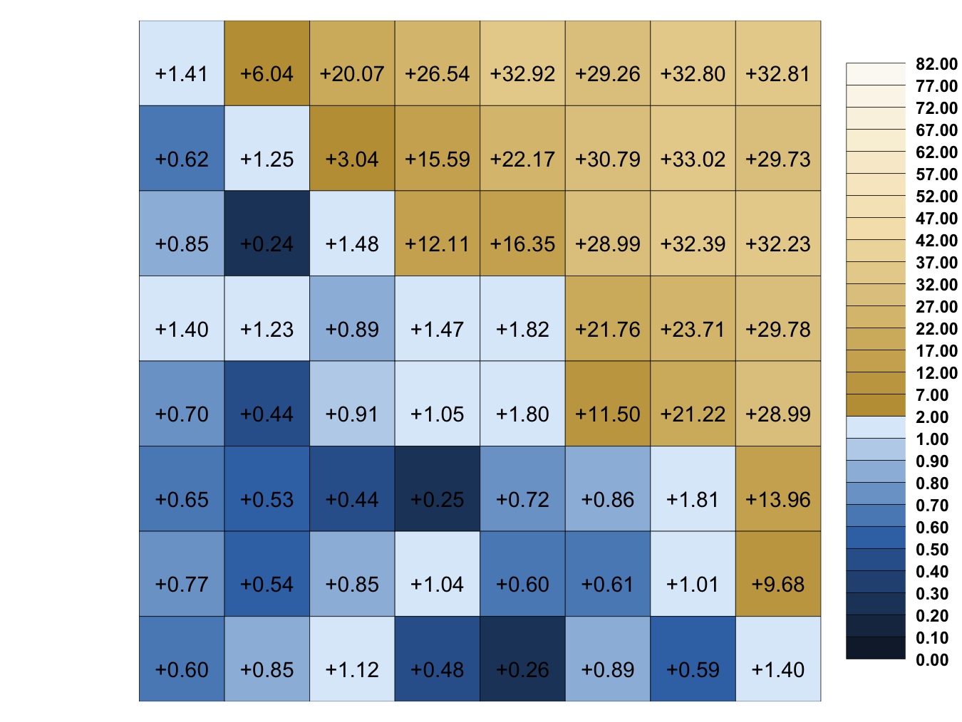
Figure 10: Simulation results for the perimeter process – $\boldsymbol{\mu}^{(1)}=(100,0)$, $\boldsymbol{\mu}^{(2)}=(0,0)$.

Since we were simulating two planar random walks, we had some freedom in the design of our simulation study, but we kept everything as simple as possible. Namely, covariance matrices were always multiples of the identity matrix, and the steps of random walks were generated from multivariate normal distribution. To see what happens in the scenario when one of the two walks has a non-zero drift, and the other one has a zero drift (illustrated in Figure 9), we set one drift vector to $(100,0)$, and the other one, clearly, to $(0,0)$. As mentioned, the covariance matrices of both walks were always of the shape $\sigma I_{2}$ (where $I_{2}$ is the two-dimensional identity matrix). We varied the value of $\sigma$ across all the elements from the set $\{0.1,0.5,1,5,10,50,100,500\}$. More precisely, for every combination of $\sigma_{1},\sigma_{2}\in\{0.1,0.5,1,5,10,50,100,500\}$ we simulated $10^{3}$ random walks with parameters $\boldsymbol{\mu}^{(1)}=(100,0)$, $\boldsymbol{\Sigma}^{(1)}=\sigma_{1}I_{2}$ and $\boldsymbol{\mu}^{(2)}=(0,0)$, $\boldsymbol{\Sigma}^{(2)}=\sigma_{2}I_{2}$. In each of those $10^{3}$ simulations, we simulated $10^{4}$ steps of both random walks, determined the convex hull generated by the trajectories of both walks, and then calculated the perimeter of the resulting convex hull. Hence, for each combination of values of $\sigma_{1}$ and $\sigma_{2}$ we had $10^{3}$ realizations of a random variable $L_{n}$, for $n=10^{4}$. We then tested those $10^{3}$ realizations for normality and calculated the $p$-value. To gain additionally stability of our simulations, we repeated the procedure $5$ times and averaged all the $p$-values obtained. Since we varied the values of $\sigma_{1}$ and $\sigma_{2}$ across $8$ different values, we ended up with $8\times 8$ matrix of averaged $p$-values. We then transformed the elements of the matrix with the mapping $x\mapsto-\log x$ so that it is easier to present the results. After this transformation, the values in the matrix that were less than or equal to $2$ corresponded to $p$-values big enough to suggest not to reject the hypothesis of Gaussian distribution. Bigger values in the matrix correspond to smaller $p$-values and point in the direction of non-Gaussian behavior. To stress this difference between values less than or equal to $2$ and values bigger than $2$, we use different color palettes for those two ranges of values. In Figure 10, as in all the figures that follow, the color on the position $(i,j)$ (starting from top left corner) corresponds to the simulation in which $\sigma_{1}$ is equal to the $i$-th value, and $\sigma_{2}$ to the $j$-th value from the set $\{0.1,0.5,1,5,10,50,100,500\}$. As one can see in Figure 10, if the variability of the zero-drift random walk is smaller than or equal to the variability of the random walk with the non-zero drift simulations suggest not to reject the hypothesis of Gaussian distribution. However, we believe that in this case the impact of the non-Gaussian part is too small to be detected by the test. As soon as the variance of the zero-drift random walk is bigger, the simulations clearly suggest non-Gaussian behavior.

For illustration, we conduct the same experiment in the case when the assumption (A1) is not violated. We can see in Figure 11 that the same design of simulation study as above captures the behavior proven in Theorem 2.6.

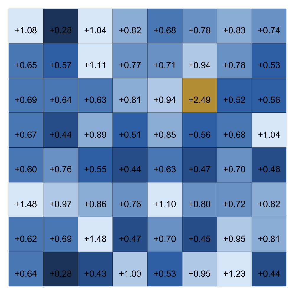
(a) $\boldsymbol{\mu}^{(1)}=(200,100)$, $\boldsymbol{\mu}^{(2)}=(-100,100)$

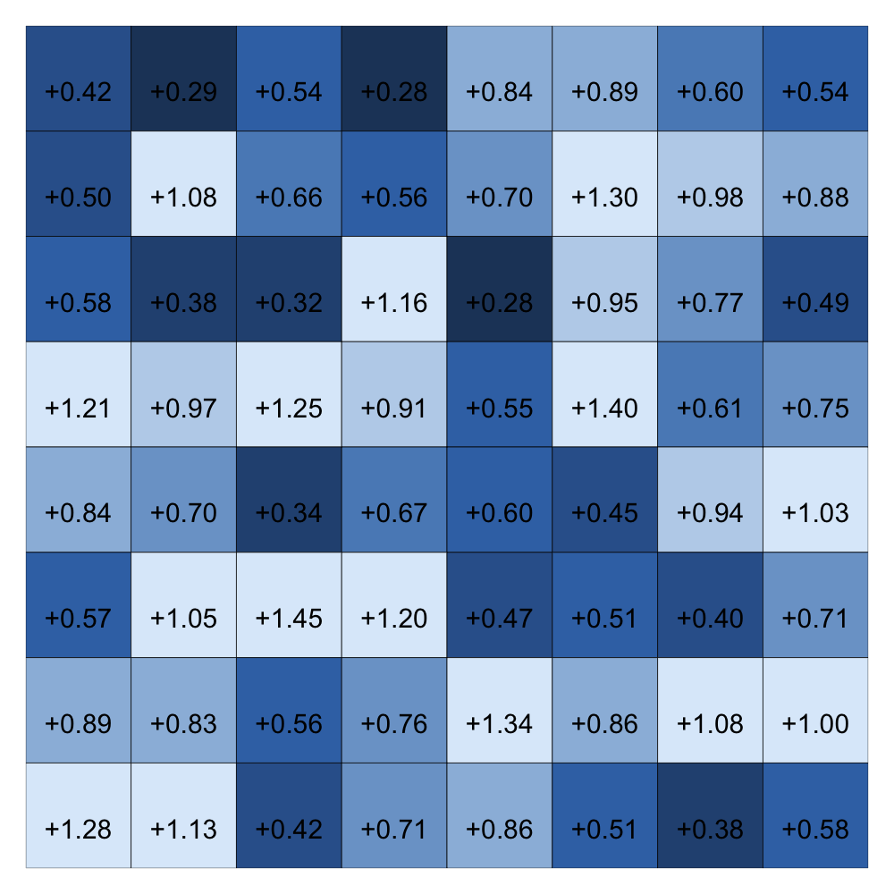
(b) $\boldsymbol{\mu}^{(1)}=(200,100)$, $\boldsymbol{\mu}^{(2)}=(100,100)$

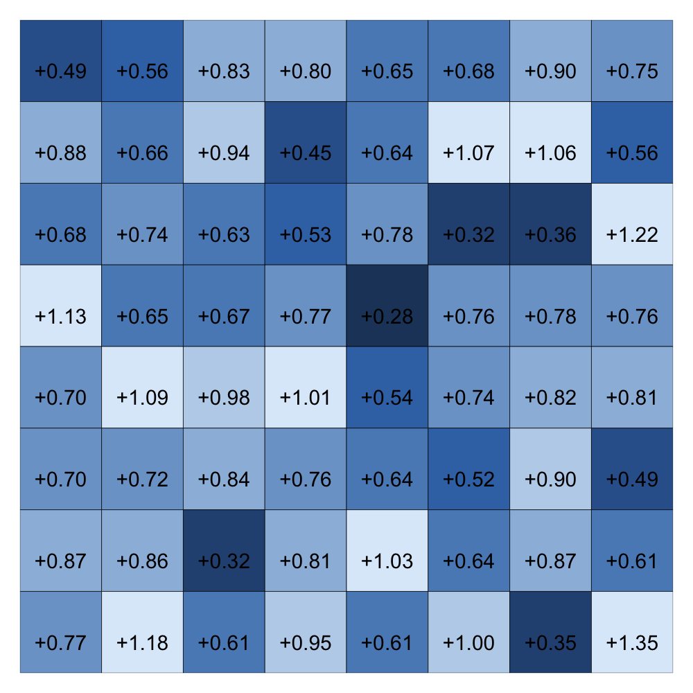
(c) $\boldsymbol{\mu}^{(1)}=(200,0)$, $\boldsymbol{\mu}^{(2)}=(-100,0)$

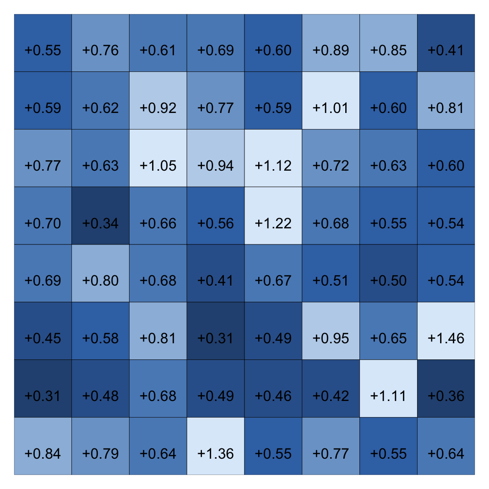
(d) $\boldsymbol{\mu}^{(1)}=(200,0)$, $\boldsymbol{\mu}^{(2)}=(100,0)$

Figure 11: Simulation results (for the perimeter process) illustrating Theorem 2.6

The last scenario in which assumption (A1) is not satisfied is the one where $\boldsymbol{\mu}^{(1)}=\boldsymbol{\mu}^{(2)}\neq\boldsymbol{0}$. It was clear to us that our approach to the proof of Theorem 2.6 cannot cover this case, but our first impression was that the normality will still hold. Hence, it was somewhat surprising to us when simulations suggested that in this case we again do not have normal behavior (see Figure 12). These simulation results motivated the formulation of the assumption (A1) in the present form. Possible justification is that one has to consider the triangle spanned by the drift vectors, and as soon as one of the three sides has length zero, the normality does not hold.

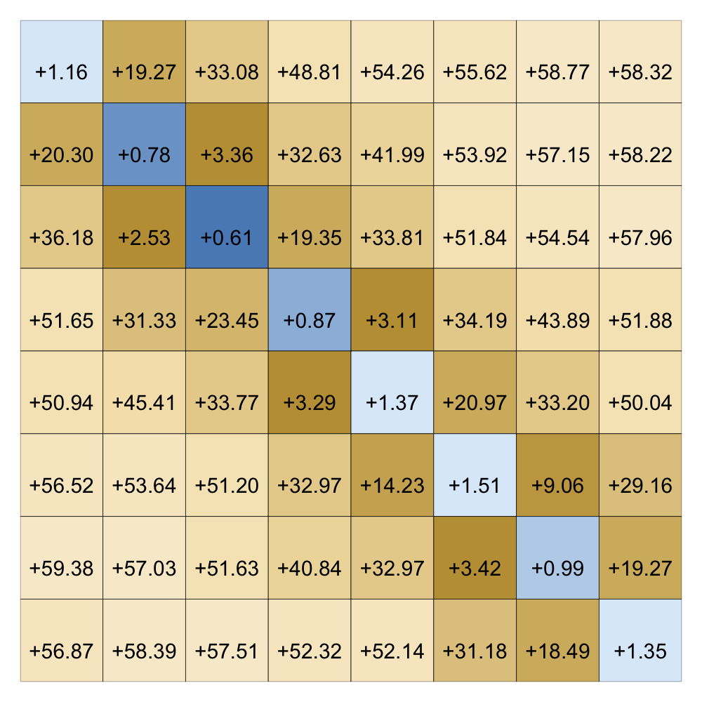
Figure 12: Simulation results for the perimeter process – $\boldsymbol{\mu}^{(1)}=(100,0)$, $\boldsymbol{\mu}^{(2)}=(100,0)$.

When it comes to the assumption (A1) in the diameter case, we have completely analogous situation as above. We repeated all the experiments as above and got analogous results (see Figure 13). However, in the central limit theorem for the diameter (Theorem 2.7) we have additional assumption (A2). Again, our method of proof did not work in this case, but our intuition was that the normality should still hold. We were quite surprised to see that simulations suggest non-Gaussian behavior when the set $\{\|\boldsymbol{\mu}^{(1)}\|,\|\boldsymbol{\mu}^{(2)}\|,\|\boldsymbol{\mu}^{(1)}-\boldsymbol{\mu}^{(2)}\|\}$ does not have a unique maximal element. Those simulation results are shown in Figure 14.

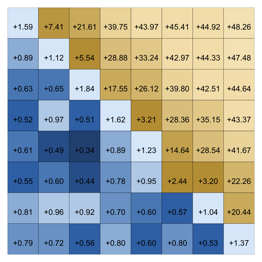
(a) $\boldsymbol{\mu}^{(1)}=(100,0)$, $\boldsymbol{\mu}^{(2)}=(0,0)$

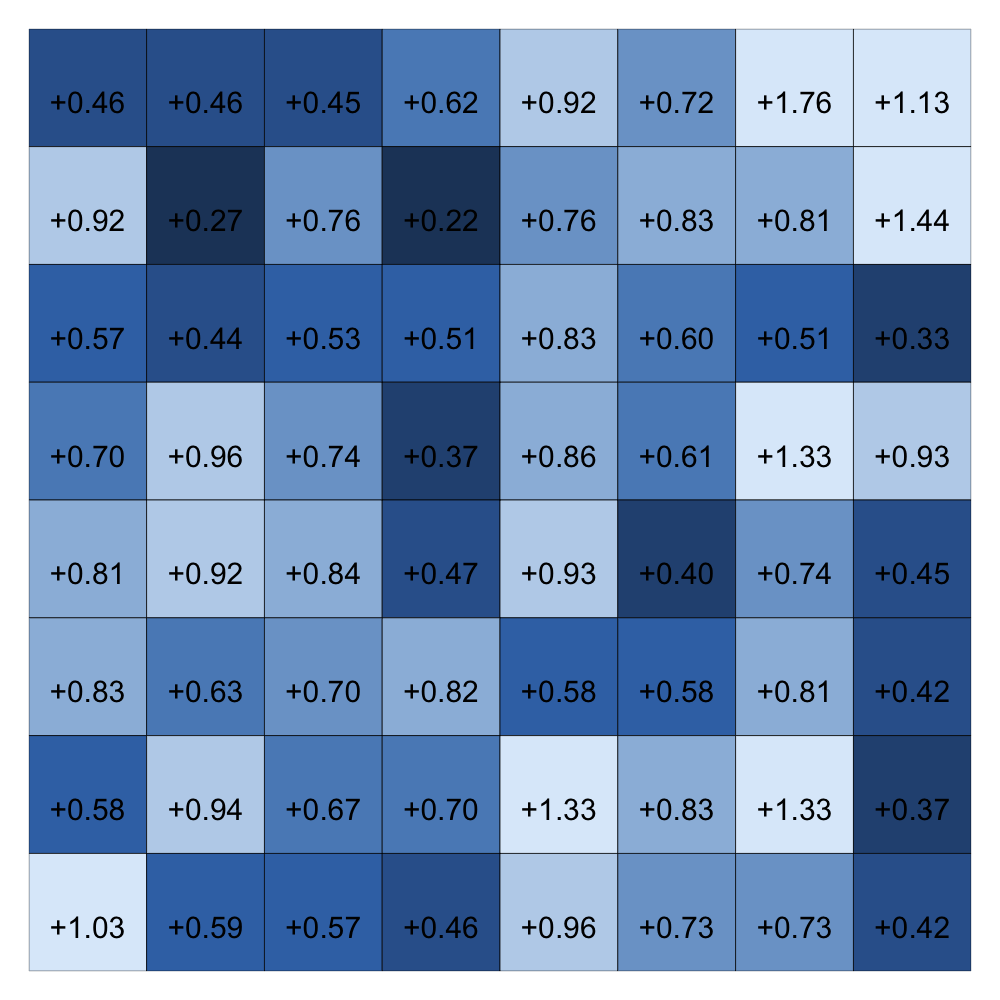
(b) $\boldsymbol{\mu}^{(1)}=(200,100)$, $\boldsymbol{\mu}^{(2)}=(-100,100)$

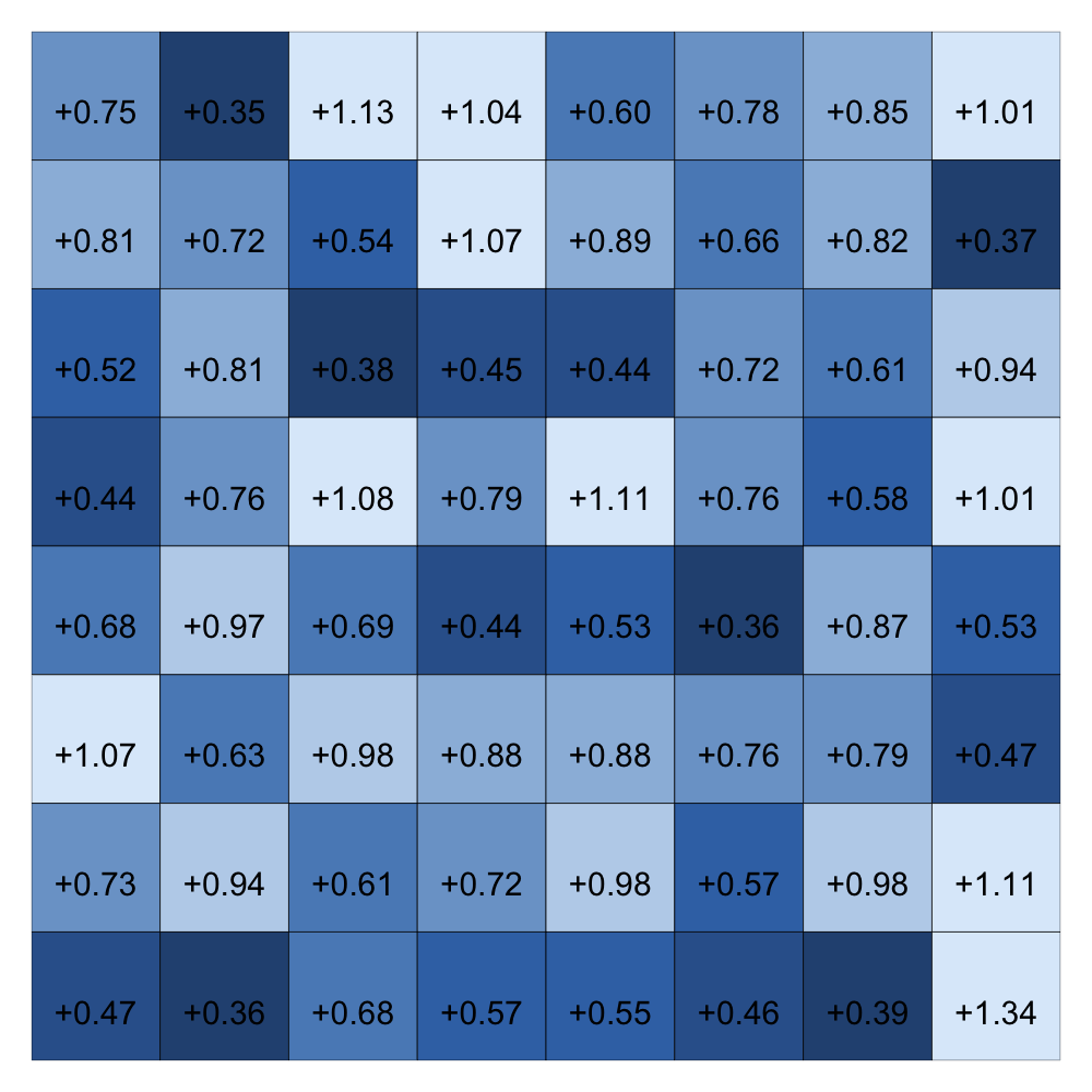
(c) $\boldsymbol{\mu}^{(1)}=(200,100)$, $\boldsymbol{\mu}^{(2)}=(100,100)$

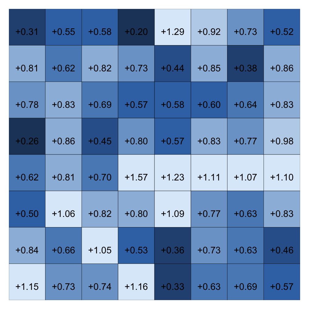
(d) $\boldsymbol{\mu}^{(1)}=(200,0)$, $\boldsymbol{\mu}^{(2)}=(-100,0)$

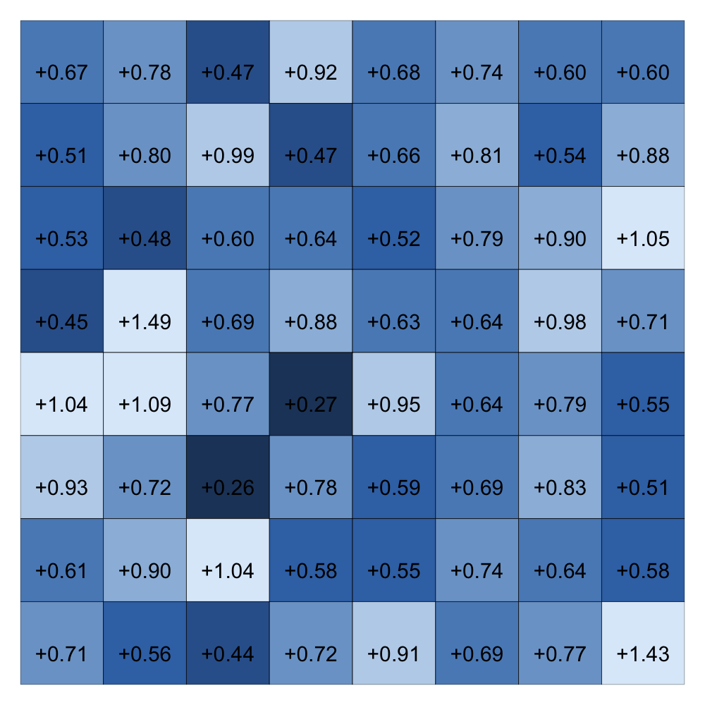
(e) $\boldsymbol{\mu}^{(1)}=(200,0)$, $\boldsymbol{\mu}^{(2)}=(100,0)$

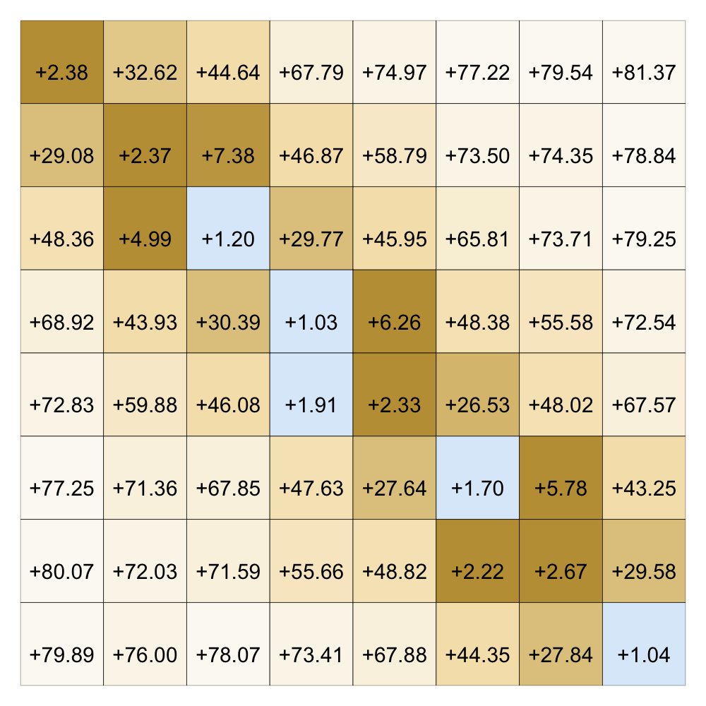
(f) $\boldsymbol{\mu}^{(1)}=(100,0)$, $\boldsymbol{\mu}^{(2)}=(100,0)$

Figure 13: Simulation results for the diameter process in the same scenarios as the ones analyzed in the context of the perimeter process.

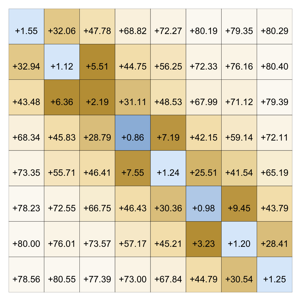
(a) $\boldsymbol{\mu}^{(1)}=(100,200)$, $\boldsymbol{\mu}^{(2)}=(-100,200)$

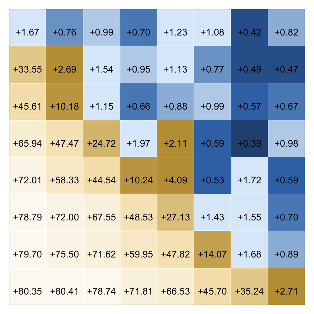
(b) $\boldsymbol{\mu}^{(1)}=(0,200)$, $\boldsymbol{\mu}^{(2)}=(200,100)$

Figure 14: Simulation results (for the diameter process) in the case when assumption (A2) is violated.

One thing that the simulations suggest is that the variability of the walks does not change the limiting behavior of the studied processes (as long as $\sigma_{L}>0$ and $\sigma_{D}>0$), but it has an effect on simulations. Therefore, it could be that because of a bad simulation study design we conjectured something that does not hold. Regardless of that, it seems that scenarios excluded with assumptions (A1) and (A2) require additional work and a different approach, and the efforts to extend our results in this direction are currently underway.

References

- [1] Adrian Baddeley, Imre Bárány, and Rolf Schneider. Random polytopes, convex bodies, and approximation. Stochastic Geometry: Lectures given at the CIME Summer School held in Martina Franca, Italy, September 13–18, 2004, pages 77–118, 2007.
- [2] Sarah A Boyle, Waldete C Lourenço, Lívia R Da Silva, and Andrew T Smith. Home range estimates vary with sample size and methods. Folia Primatologica, 80(1):33–42, 2008.
- [3] Gunnar Claussen, Alexander K Hartmann, and Satya N Majumdar. Convex hulls of random walks: Large-deviation properties. Physical Review E, 91(5):052104, 2015.
- [4] Wojciech Cygan, Nikola Sandrić, and Stjepan Šebek. Convex hulls of stable random walks. Electron. J. Probab., 27:Paper No. 98, 30, 2022.
- [5] Wojciech Cygan, Nikola Sandrić, Stjepan Šebek, and Andrew Wade. Iterated-logarithm laws for convex hulls of a random walks with drift, 2023.
- [6] James Davidson. Stochastic limit theory: An introduction for econometricians. OUP Oxford, 1994.
- [7] Timo Dewenter, Gunnar Claussen, Alexander K Hartmann, and Satya N Majumdar. Convex hulls of multiple random walks: A large-deviation study. Physical Review E, 94(5):052120, 2016.
- [8] Rick Durrett. Probability: theory and examples, volume 49. Cambridge University Press, 2019.
- [9] Ronen Eldan. Extremal points of high-dimensional random walks and mixing times of a Brownian motion on the sphere. Ann. Inst. Henri Poincaré Probab. Stat., 50(1):95–110, 2014.
- [10] Ronen Eldan. Volumetric properties of the convex hull of an -dimensional Brownian motion. Electron. J. Probab., 19:no. 45, 34, 2014.
- [11] Luca Giuggioli, Guillermo Abramson, VM Kenkre, RR Parmenter, and TL Yates. Theory of home range estimation from displacement measurements of animal populations. Journal of Theoretical Biology, 240(1):126–135, 2006.
- [12] Peter M Gruber. Convex and discrete geometry, volume 336. Springer, 2007.
- [13] Allan Gut. Probability: a graduate course, volume 200. Springer, 2006.
- [14] Zakhar Kabluchko, Vladislav Vysotsky, and Dmitry Zaporozhets. Convex hulls of random walks: expected number of faces and face probabilities. Adv. Math., 320:595–629, 2017.
- [15] Zakhar Kabluchko, Vladislav Vysotsky, and Dmitry Zaporozhets. Convex hulls of random walks, hyperplane arrangements, and Weyl chambers. Geom. Funct. Anal., 27(4):880–918, 2017.
- [16] Chak Hei Lo, James McRedmond, and Clare Wallace. Functional limit theorems for random walks, 2018.
- [17] Satya N. Majumdar, Alain Comtet, and Julien Randon-Furling. Random convex hulls and extreme value statistics. J. Stat. Phys., 138(6):955–1009, 2010.
- [18] James McRedmond. Convex hulls of random walks, 2019.
- [19] James McRedmond and Andrew R. Wade. The convex hull of a planar random walk: perimeter, diameter, and shape. Electron. J. Probab., 23:Paper No. 131, 24, 2018.
- [20] James McRedmond and Chang Xu. On the expected diameter of planar Brownian motion. Statist. Probab. Lett., 130:1–4, 2017.
- [21] Dennis D Murphy and Barry R Noon. Integrating scientific methods with habitat conservation planning: reserve design for northern spotted owls. Ecological Applications, 2(1):3–17, 1992.
- [22] Joseph Rudnick and George Gaspari. The shapes of random walks. Science, 237(4813):384–389, 1987.
- [23] Rolf Schneider. Convex bodies: the Brunn–Minkowski theory. Number 151. Cambridge university press, 2014.
- [24] Rolf Schneider and John André Wieacker. Approximation of convex bodies by polytopes. Bulletin of the London Mathematical Society, 13(2):149–156, 1981.
- [25] Timothy Law Snyder and J. Michael Steele. Convex hulls of random walks. Proc. Amer. Math. Soc., 117(4):1165–1173, 1993.
- [26] F. Spitzer and H. Widom. The circumference of a convex polygon. Proc. Amer. Math. Soc., 12:506–509, 1961.
- [27] Konstantin Tikhomirov and Pierre Youssef. When does a discrete-time random walk in absorb the origin into its convex hull? Ann. Probab., 45(2):965–1002, 2017.
- [28] Vladislav Vysotsky and Dmitry Zaporozhets. Convex hulls of multidimensional random walks. Trans. Amer. Math. Soc., 370(11):7985–8012, 2018.
- [29] Andrew R. Wade and Chang Xu. Convex hulls of planar random walks with drift. Proc. Amer. Math. Soc., 143(1):433–445, 2015.
- [30] Andrew R. Wade and Chang Xu. Convex hulls of random walks and their scaling limits. Stochastic Process. Appl., 125(11):4300–4320, 2015.
- [31] Bruce J Worton. A convex hull-based estimator of home-range size. Biometrics, pages 1206–1215, 1995.
- [32] Chang Xu. Convex hulls of planar random walks, 2017.