Mean temperature and concentration profiles in
turbulent internal flows

Abstract

We derive explicit formulas for the mean profiles of temperature or concentration of a diffusing substance (modeled as passive scalars) in forced turbulent convection, as a function of the Reynolds and Prandtl numbers. The derivation leverages on the observed universality of the inner-layer thermal eddy diffusivity with respect to Reynolds and Prandtl number variations and across different flows, and on universality of the passive scalar defect in the core flow. Matching of the inner- and outer-layer expression yields a smooth compound passive scalar profile. We find excellent agreement of the analytical profile with data from direct numerical simulations of pipe and channel flows under various forcing conditions, and over a wide range of Reynolds and Prandtl numbers.

1 Introduction

The exploration of passive scalars within turbulent flows bounded by walls holds significant practical implications. It plays a crucial role in comprehending the behavior of diluted contaminants and serves as a model for temperature distribution assuming low Mach numbers and minimal temperature disparities [1, 2]. Nonetheless, quantifying the concentration of passive tracers and minute temperature differences poses formidable challenges, leading to restricted insights into fundamental passive scalar statistics [3, 4, 5, 6].

The investigation of passive scalars in turbulent flows predominantly centers on scenarios where the Prandtl number ($\mathrm{Pr}$) approaches unity, representing the ratio of kinematic viscosity to thermal diffusivity ($\mathrm{Pr}=\nu/\alpha$). Numerous studies have discussed the close similarities between the passive scalar field and the streamwise velocity field under these conditions [7, 8, 9]. However, various fluids, including water, engine oils, glycerol, and polymer melts, exhibit Prandtl numbers significantly exceeding unity, while liquid metals and molten salts have markedly lower Prandtl numbers.

For the diffusion of contaminants, the role of the Prandtl number is supplanted by the Schmidt number, which denotes the ratio of kinematic viscosity to mass diffusivity. In practical applications, the Schmidt number typically far exceeds unity [10]. In such instances, the resemblance between velocity and passive scalar fluctuations is significantly compromised, rendering predictions of even fundamental flow properties notably challenging.

Regarding wall fluxes, the most robust framework established to date is attributed to the work by Kader and Yaglom [11]. Drawing upon universality arguments, these authors derived a predictive law for the nondimensional flux (Nusselt number) as a function of the Prandtl number. This framework primarily involves modeling the logarithmic offset function, which represents the Prandtl-dependent additive constant in the overlap-layer mean passive scalar profiles. Despite the solidity of this framework, semi-empirical power-law correlations [12, 13] continue to find widespread usage in engineering design. As for the mean profiles of passive scalars, the most comprehensive study available can be traced back to the work of Kader [4]. In this study, an empirical interpolation formula was derived, connecting the universal near-wall conductive layer with the outer logarithmic layer. This interpolation formula was observed to reasonably align with the temperature profile behavior observed in experiments available at the time.

Pirozzoli [14] studied the statistics of passive scalars in pipe flow in the range of Prandtl numbers from $\mbox{{Pr}}=0.00625$ to $\mbox{{Pr}}=16$, using direct numerical simulation (DNS) of the Navier–Stokes equations, and found that the mean passive scalar profiles at $\mbox{{Pr}}\gtrsim 0.0125$ exhibit logarithmic overlap layers, and universal parabolic distributions in the core part of the flow. A model of the eddy viscosity was used to derive semi-analytical predictions (numerical quadrature was required) for the mean passive scalar profiles, and for the corresponding logarithmic offset function. Asymptotic scaling formulas were also derived for the thickness of the diffusive sub-layer, and the heat transfer coefficient, which are capable of accounting accurately for variations with both the Reynolds and the Prandtl number, for $\mbox{{Pr}}\gtrsim 0.25$. In this paper, we use the same DNS database, with the goal of deriving fully explicit analytical representations for the mean passive scalar profiles and the corresponding wall fluxes, as a function of the Reynolds and Prandtl numbers. Although, as previously pointed out, the study of passive scalars is relevant in several contexts, one of the primary fields of application is heat transfer, and therefore from now on we will refer to the passive scalar field as the temperature field (denoted as $T$), and passive scalar fluxes will be interpreted as heat fluxes.

2 Predictive formulas

2.1 The inner layer

The starting point for the analysis of the mean temperature profile in the inner layer is the mean thermal balance equation, which in internal flows reads

$$\frac{1}{\mbox{{Pr}}}\frac{\mbox{d}\Theta^{+}}{\mbox{d}y^{+}}-\left<v\theta\right>^{+}=1-\eta,$$ (1)

where $\theta=T-T_{w}$ expresses the temperature difference with respect to the wall, $v$ is the wall-normal velocity, $\eta=y/\delta_{t}$, with $y$ the wall distance, and $\delta_{t}$ a suitable measure of the thickness of the thermal layer, to be identified from case to case as later explained. Here and in the following, capital symbols are used to denote Reynolds averaged quantities, whereas lowercase symbols are used to denote fluctuations thereof, and angle brackets denote the averaging operator. In equation (1) the $+$ superscript denotes normalization in wall units, whereby the friction velocity ($u_{\tau}=(\tau_{w}/\rho)^{1/2}$) is used for velocities, the viscous length scale ($\delta_{v}=\nu/u_{\tau}$) is used for lengths, and the friction temperature ($T_{\tau}=\alpha/u_{\tau}\left(\mbox{d}\langle T\rangle/\mbox{d}y\right)_{w}$) is used for temperature. The mean wall shear stress is $\tau_{w}$, and $\rho$ and $\nu$ and the fluid density and viscosity, respectively.

Modeling the turbulent heat flux $\left<v\theta\right>$ in (1) requires closure with respect to the mean temperature gradient [see, e.g. 2], through the introduction of a thermal eddy diffusivity, defined as

$$\alpha_{t}=\frac{\left<u_{r}\theta\right>}{\mbox{d}\Theta/\mbox{d}y}.$$ (2)

As noted by Pirozzoli [15], the thermal eddy diffusivity in the inner layer of wall-bounded flows has a relatively simple behavior, and it is very nearly universal with respect to variations of the Reynolds number. The thermal eddy diffusivity is also very much insensitive to variations of the Prandtl number, with exception of vanishingly small Prandtl numbers, in which limit $\alpha_{t}$ must vanish as conduction takes over. This is well portrayed in figures 1 and 4, which we will comment later on.

Noting that asymptotic arguments [11] suggest the limiting near-wall behaviour to be $\alpha_{t}\sim y^{3}$, whereas the presence of a logarithmic layer in the mean temperature profile implies $\alpha_{t}\sim y$ away from the wall, Pirozzoli [15] suggested the following functional expression to model the thermal eddy viscosity throughout the inner layer

$$\alpha_{t}^{+}=\frac{(k_{\theta}{y^{+}})^{3}}{(k_{\theta}{y^{+}})^{2}+C_{\theta}^{2}}.$$ (3)

Equation (3) is inspired by the work of Musker [16], who used a similar function to model the eddy viscosity in turbulent boundary layers. In equation (3) the thermal Kármán constant was determined to be $k_{\theta}\approx 0.459$ [17], and $C_{\theta}=10.0$ was found based on scrutiny of DNS data for pipe flow. Whereas alternative functional expressions are possible, equation (3) bears the substantial advantage of being amenable to further analytical developments.

Starting from equation (1) and under the near-wall approximation ($\eta<<1$), one can infer the distribution of the mean temperature in the inner layer from knowledge of the eddy thermal diffusivity, by integrating

$$\frac{\mbox{d}\Theta^{+}}{\mbox{d}y^{+}}=\frac{\mbox{{Pr}}}{1+\mbox{{Pr}}\,\alpha_{t}^{+}},$$ (4)

with $\alpha_{t}$ given in equation (3). The result of the integration yields the mean temperature profile in the inner layer

$$\begin{split}\Theta_{i}^{+}(y^{+},\mbox{{Pr}})=\frac{1}{2k_{\theta}\zeta_{0}(2+3\mbox{{Pr}}\zeta_{0})}\left\{\frac{2\left(2\zeta_{0}+3\mbox{{Pr}}^{2}C_{\theta}^{2}\zeta_{0}+\mbox{{Pr}}(C_{\theta}^{2}+2\zeta_{0}^{2})\right)}{\Delta}\right.\\ \times\left[\arctan{\left(\frac{1+\mbox{{Pr}}\zeta_{0}}{\Delta}\right)}\right.-\left.\arctan{\left(\frac{1+\mbox{{Pr}}(2\zeta+\zeta_{0})}{\Delta}\right)}\right]\\ +2\mbox{{Pr}}\left(C^{2}+\zeta_{0}^{2}\right)\log(1-\frac{\zeta}{\zeta_{0}})\\ +\left.\vphantom{\frac{2\left(2\zeta_{0}+3\mbox{{Pr}}^{2}C_{\theta}^{2}\zeta_{0}+\mbox{{Pr}}(C_{\theta}^{2}+2\zeta_{0}^{2})\right)}{\Delta}}\left(\mbox{{Pr}}(2\zeta_{0}^{2}-C_{\theta}^{2})+2\zeta_{0}\right)\log{\frac{\mbox{{Pr}}\zeta^{2}+(1+\mbox{{Pr}}\zeta_{0})(\zeta+\zeta_{0})}{\zeta_{0}(1+\mbox{{Pr}}\zeta_{0})}}\right\},\end{split}$$ (5)

where $\zeta=k_{\theta}y^{+}$, $\Delta=(3\mbox{{Pr}}^{2}\zeta_{0}^{2}+2\mbox{{Pr}}\zeta_{0}-1)^{1/2}$, and $\zeta_{0}$ is the single (negative) real root of the cubic equation

$$\mbox{{Pr}}\zeta^{3}+\zeta^{2}+C_{\theta}^{2}=0,$$ (6)

whose exact solution is

$$\zeta_{0}=\frac{1}{3\mbox{{Pr}}}\left(-1+\frac{1}{z}+z\right),z=\left[\frac{1}{2}\left(-2-27\mbox{{Pr}}^{2}C_{\theta}^{2}+\sqrt{-4+\left(2+27\mbox{{Pr}}^{2}C_{\theta}^{2}\right)^{2}}\right)\right]^{1/3}.$$ (7)

The temperature profiles given in equation (5) exhibit logarithmic behaviour at $y^{+}>>1$, namely

$$\Theta^{+}=\frac{1}{k_{\theta}}\log y^{+}+\beta(\mbox{{Pr}}),$$ (8)

where the log-law offset function is given by the following asymptotic expression

$$\beta(\mbox{{Pr}})=\frac{1}{k_{\theta}}\left[\frac{2\pi C_{\theta}^{2/3}}{3\sqrt{3}}\mbox{{Pr}}^{2/3}+\frac{1}{3}\log\mbox{{Pr}}-\left(\frac{1}{6}+\frac{1}{2\sqrt{3}}+\frac{2}{3}\log C_{\theta}-\log k_{\theta}\right)\right]+O(\mbox{{Pr}}^{-2/3}).$$ (9)

Other synthetic profiles for the mean temperature in the inner layer are available in the literature. A notable example is the approach described by Cebeci and Bradshaw [2], where the authors used the eddy-diffusivity and eddy-viscosity formulas from classical turbulence models to derive temperature profiles at arbitrary Prandtl numbers. Another example is the empirical correlations based on experimental-data fitting proposed by Kader [4], which we use as reference in study. The main advantage of the present framework compared to existing formulas is that equation (5) provides an explicit analytical expression for the mean temperature profiles based on a simple expression for the eddy diffusivity, which embeds the correct asymptotic behavior close to the wall and in the logarithmic layer.

2.2 The core layer

The behavior of the mean temperature in the core (wake) region of wall-bounded flows was studied in terms of the temperature defect function by Pirozzoli et al. [18] and Pirozzoli et al. [19]. The key finding was that the temperature defect profile (with respect to the peak value) is very nearly universal with respect to both Reynolds and Prandtl number variations, and the universal region encompasses a wide part of the flow thickness. Departures from outer-layer universality were only observed at $\mbox{{Pr}}\lesssim 0.025$, below which the similarity region becomes progressively confined to the outermost part of the thermal wall layer. As suggested by Pirozzoli et al. [18, 17], the core temperature profiles in internal flows can be closely approximated with simple universal quadratic distributions, which one can derive from (1) under the assumption of constant eddy thermal diffusivity. This assumption is analogous to the hypothesis of constant eddy viscosity proposed by Clauser [20], also leading to a parabolic outer layer velocity distribution. A convenient analytical representation for the core mean temperature profile $\Theta_{c}$ is then

$$\Theta_{{}_{e}}^{+}-\Theta_{c}^{+}=C_{w}\left(1-\eta\right)^{2},$$ (10)

where $\Theta_{{}_{e}}$ is the value of the mean temperature at the edge of the thermal wall layer.

2.3 Patching

An explicit approximation for the mean temperature profile throughout the thermal wall layer is then obtained by patching the inner-layer profile (5) with the core profile  (10). Smooth patching is obtained by setting the transition point at the wall distance where the asymptotic logarithmic profile (8) and the core temperature profile (10) match and have equal first derivative. It is easy to show that continuity of the first derivatives is achieved provided the patching point is placed at the coordinate

$$\eta^{*}=\left.\left(1-\sqrt{1-\frac{2}{C_{w}k_{\theta}}}\right)\right/2,$$ (11)

whereas matching the values of the inner-layer and core temperature profiles implies that

$$\Theta_{e}^{+}=\Theta_{i}^{+}(\eta^{*}\delta_{t}^{+},\mbox{{Pr}})+C_{w}\left(1-\eta^{*}\right)^{2},$$ (12)

to be used in equation (10).

Flow	Heating	$\delta_{t}$	$C_{\theta}$	$C_{w}$	$\eta^{*}$
Pipe	UIH	$R$	10.0	6.00	0.238
Pipe	CHF	$R$	10.0	7.00	0.193
Channel	UIH-sym	$h$	10.0	5.48	0.274
Channel	UIH-asym	$2h$	10.0	12.3	0.0982

Table 1: Parameters for compound mean temperature profiles obtained by patching equation (5) and (10). $\delta_{t}$ is the assumed thickness of the thermal layer, with $R$ the pipe radius and $h$ the channel half-thickness. $C_{\theta}$ is the inner-layer constant to be used in (3), $C_{w}$ is the core profile constant to use in (10), and $\eta^{*}$ is the outer-scaled coordinate of the patching point between the inner and the core temperature profiles.

3 Results

3.1 Pipe flow

Pr	Mesh ($N_{z}\times N_{r}\times N_{\phi}$)	$\mbox{{Pe}}_{\tau}$	$\mbox{{Nu}}_{UIH}$	$\mbox{{Nu}}_{CHF}$	Line style
0.00625	$1792\times 164\times 1793$	7.11	$8.02$	7.35
0.0125	$1792\times 164\times 1793$	14.2	$9.41$	8.68
0.025	$1792\times 164\times 1793$	28.5	$12.6$	11.6
0.0625	$1792\times 164\times 1793$	71.1	$21.5$	20.2
0.125	$1792\times 164\times 1793$	142.2	$34.2$	32.5
0.25	$1792\times 164\times 1793$	284.4	$53.8$	51.4
0.5	$1792\times 164\times 1793$	568.8	$81.7$	79.0
1	$1792\times 164\times 1793$	1137.6	$119.9$	116.6
2	$3584\times 269\times 3584$	2275.2	$168.0$	165.0
4	$3584\times 269\times 3584$	4550.4	$233.3$	229.7
16	$7168\times 441\times 7168$	18201.6	$421.2$	419.4

Table 2: Flow parameters for DNS of pipe flow at various Prandtl number. $N_{z}$, $N_{r}$, $N_{\phi}$ denote the number of grid points in the axial, radial, and azimuthal directions, respectively; $\mbox{{Pe}}_{\tau}=\mbox{{Pr}}\,\mbox{{Re}}_{\tau}$ is the friction Péclet number; Nu is the Nusselt number (as defined in equation (13)), for cases with uniform internal heating (UIH), and constant heat flux (CHF). All DNS are carried out in a computational domain with length $L_{z}=15R$, at bulk Reynolds number $\mbox{{Re}}_{b}=44000$, corresponding to friction Reynolds number $\mbox{{Re}}_{\tau}\approx 1138$.

Results of DNS of thermal pipe flow are reported for the two canonical cases of uniform internal heating (UIH), and constant heat flux (CHF). In the former case the energy equation is forced with a spatially uniform internal heating term, in such a way that the bulk temperature is kept constant in time [18]. In the latter case, the forcing term varies from point to point proportionally to $u/u_{b}$, such that the bulk temperature is also constant [21, 22, 23]. This second approach more precisely mimics the physical case of thermally developed flow in a duct with spatially and temporally uniform wall heating [2]. As discussed by Abe et al. [22], Alcántara-Ávila et al. [23], the forcing strategy has small, but non-negligible effect on the temperature statistics. In both cases, the maximum temperature is attained at the pipe centreline, hence we assume the thermal wall layer thickness to be the pipe radius, and accordingly set $\delta_{t}=R$.

A wide range of Reynolds and Prandtl numbers has been explored, with spanning Prandtl numbers from 0.0025 to 16 and friction Reynolds numbers $\mbox{{Re}}_{\tau}(=Ru_{\tau}/\nu)$ ranging from $180$ to $6000$ [17, 14]. A full scan of Prandtl numbers is here reported, for fixed bulk Reynolds number $\mbox{{Re}}_{b}=44000$, corresponding to friction Reynolds number $\mbox{{Re}}_{\tau}\approx 1138$. The corresponding computational parameters are reported for reference in table 2. In the table we also report some key global parameters as the friction Péclet number, $\mbox{{Pe}}_{\tau}=\mbox{{Pr}}\mbox{{Re}}_{\tau}$, and the Nusselt number,

$$\mbox{{Nu}}=\mbox{{Re}}_{b}\,\mbox{{Pr}}\,\mbox{{St}},$$ (13)

with St the Stanton number, defined as

$$\mbox{{St}}=\frac{\alpha\left<\frac{\mbox{d}{T}}{\mbox{d}y}\right>_{w}}{u_{b}\left(T_{m}-T_{w}\right)},$$ (14)

where $u_{b}$ is the bulk velocity and $T_{m}$ is the mixed mean temperature [13]. The table supports the generally accepted notion that the specific forcing has little effect of the global thermal performance at Prandtl number of order unity or higher, however percent differences in the Nusselt number become significant at low Prandtl numbers.

(a)  (b) 

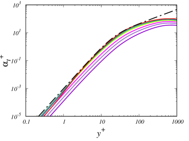
Figure 1: Distributions of inferred eddy thermal diffusivity ($\alpha_{t}$) as a function of wall distance for pipe flow with uniform internal heating (a) and constant heat flux (b), at various Pr, for $\mbox{{Re}}_{\tau}=1138$. The dash-dotted line denotes the fit given in equation (3). Colour codes are as in table 2.

The inferred eddy thermal diffusivities for all cases at $\mbox{{Re}}_{\tau}=1138$ are reported in figure 1. The agreement with the fit given in equation (3) is quite good in the inner layer, with deviations occurring only at $\mbox{{Pr}}\lesssim 0.025$. Slight deviations from the DNS are found at $y^{+}\lesssim 10$, where in any case the eddy diffusivity is much less than the molecular one. Notably, the influence of the thermal forcing (compare the two panels) seems to be entirely negligible. Universality with respect to Reynolds number variations has also been verified, but figures are omitted.

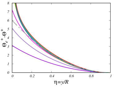
(a)  (b) 

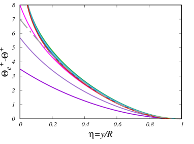
Figure 2: Mean temperature defect profiles for pipe flow with uniform internal heating (a) and constant heat flux (b), at various Pr, for $\mbox{{Re}}_{\tau}=1138$. The dot-dashed line marks a parabolic fit of the DNS data ($\Theta^{+}_{{}_{e}}-\Theta_{c}^{+}=C_{w}(1-\eta)^{2}$), with values of $C_{w}$ given in table 1. Colour codes are as in table 2.

As for the temperature distribution in the core flow, in figure 2 we show the mean temperature profiles in defect form, referred to the pipe centerline properties. Again, the temperature profiles at fixed $\mbox{{Re}}_{\tau}$ are shown at various Prandtl numbers. As claimed in previous studies [14], the figure supports close universality of the defect temperature profiles, for $\eta=y/R\gtrsim 0.2$. Furthermore, the figure confirms that the DNS data can be accurately fitted with the quadratic relationship (10). The fitting constant $C_{w}$, reported in table 1 is a bit larger for the case of CHF forcing, on account of a stronger temperature defect. The universality of defect temperature profiles concerning variations in Reynolds number has been corroborated in prior literature [17], and is not reiterated here.

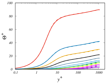
(a)  (b) 

Figure 3: Comparison of mean temperature profiles obtained from DNS (solid lines) with the prediction of the compound fitting function given by (5) and (10), with fitting parameters listed in table 1 (dashed lines), for pipe flow with uniform internal heating (a) and with constant heat flux (b), at $\mbox{{Re}}_{\tau}=1138$. The circles depicted in panel (b) represent the empirical predictions put forth by Kader [4]. Colour codes are as in table 2.

Based on the observed universality of the inner and outer layers with respect to Reynolds and Prandtl number variations, we proceed to apply the patching procedure outlined in § 2.3, with fitting parameters listed in table 1. The resulting temperature profiles are reported in figure 3, which confirms that the quality of the resulting patched temperature profiles is generally very good. Visible deviations are only evident at extremely low Prandtl numbers, as anticipated due to the absence of a genuine overlap layer. Discrepancies from the predicted trends are observed specifically at the lowest Prandtl numbers, which, as previously noted, deviate from the universal trend of $\alpha_{t}$. In panel (b), we additionally present a comparison with the empirical correlation proposed by Kader [4]. To maintain clarity, only cases with $\mbox{{Pr}}\geq 1$ are depicted. While the overall quality of the fit is satisfactory, an anomalous behavior is noticed in the buffer layer, and the shift in the log-law is somewhat overestimated at high Pr.

3.2 Channel flow

Pr	Mesh ($N_{x}\times N_{y}\times N_{z}$)	$\mbox{{Pe}}_{\tau}$	$\mbox{{Nu}}_{SYM}$	$\mbox{{Nu}}_{ASYM}$	Line style
$0.025$	$1536\times 298\times 2304$	$24.7$	10.0	5.88
$0.25$	$1536\times 298\times 2304$	$247.3$	44.6	32.7
$0.5$	$1536\times 298\times 2304$	$494.4$	68.5	53.3
$1$	$1536\times 298\times 2304$	$1002.1$	101.7	86.3
$2$	$3072\times 485\times 4608$	$2010.4$	148.7	128.9
$4$	$3072\times 485\times 4608$	$4019.6$	207.9	187.8

Table 3: Flow parameters for DNS of channel flow at various Prandtl number. $N_{x}$, $N_{y}$, $N_{z}$ denote the number of grid points in the streamwise, wall-normal, and spanwise directions, respectively; $\mbox{{Pe}}_{\tau}=\mbox{{Pr}}\,\mbox{{Re}}_{\tau}$ is the friction Péclet number; Nu is the Nusselt number (as defined in equation (13)), for cases with symmetric heating (SYM), and asymmetric heating with one adiabatic wall (ASYM). All DNS are carried out in a computational domain with size $6\pi h\times 2h\times 2\pi h$, at bulk Reynolds number $\mbox{{Re}}_{b}=40000$, corresponding to friction Reynolds number $\mbox{{Re}}_{\tau}\approx 1002$.

A similar analysis is herein reported for thermal channel flow, based on the DNS data of Pirozzoli and Modesti [24]. Two cases of thermal forcing are considered with uniform internal heating, whereby the two walls of the channel are either kept at the same temperature, hence heat is allowed to flow away through both walls, or one of the two walls is kept adiabatic. In the first case, referred to as symmetric heating (SYM), the maximum temperature is attained at the channel centreline, hence we assume the thermal wall layer thickness to be the channel half-thickness, $\delta_{t}=h$. In the second case, referred to as asymmetric heating (ASYM), the maximum temperature is attained at the adiabatic wall, hence we assume the thermal wall layer thickness to be the full channel thickness, $\delta_{t}=2h$. Just as for pipe flow, a relatively wide range of Reynolds and Prandtl numbers has been explored, with $\mbox{{Re}}_{\tau}(=hu_{\tau}/\nu)$ from 180 to 2000, and Pr from 0.025 to 4. A full scan of Prandtl numbers is here reported, for fixed bulk Reynolds number $\mbox{{Re}}_{b}(=2hu_{b}/\nu)=40000$, corresponding to friction Reynolds number $\mbox{{Re}}_{\tau}\approx 1002$. The key parameters for the DNS of channel flow are listed in table 3.

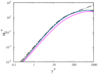
(a)  (b) 

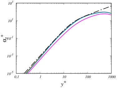
Figure 4: Distributions of inferred eddy thermal diffusivity ($\alpha_{t}$) as a function of wall distance, for plane channel flow with symmetric heating (a), and with asymmetric heating (b), at various Pr, for $\mbox{{Re}}_{\tau}=1002$. The dash-dotted line denotes the fit given in equation (3). Colour codes are as in table 3.

Figure 4 confirms that the inner-scaled thermal eddy diffusivity is universal across the range of Prandtl numbers under scrutiny, the only outlier being the case at the lowest Pr. In agreement with pipe flow, we find that equation (3) provides an excellent fit of the DNS data in the inner layer, corroborating universality of the model for the temperature log-law shift function introduced by Pirozzoli [15], and whose validity was also proved for turbulent boundary layers [25].

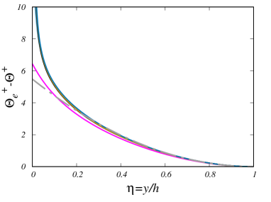
(a)  (b) 

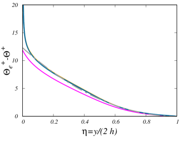
Figure 5: Mean temperature defect profiles for channel flow with symmetric heating (a), and with asymmetric heating (b), at various Pr, for $\mbox{{Re}}_{\tau}=1002$. The dot-dashed line marks a parabolic fit of the DNS data ($\Theta^{+}_{{}_{e}}-\Theta_{c}^{+}=C_{w}(1-\eta)^{2}$), with values of $C_{w}$ given in table 1. Colour codes are as in table 3.

The mean temperature defect profiles are shown in figure 5. In this respect, we note that the reference value is the mean temperature at the channel centreline in the case with symmetric heating (left panel), and the mean temperature at the adiabatic wall in the case of asymmetric heating (right panel). Just like the case of pipe flow, the simple quadratic fit (10), with suitably adjusted wake strength constants as given in table 1 yields an excellent approximation for the temperature defect, the only outlier being the case at the lowest Pr. It is especially noteworthy that in the case of asymmetric heating the quadratic approximation fits accurately the DNS data in about $90\%$ of the channel thickness.

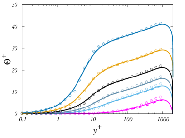
(a)  (b) 

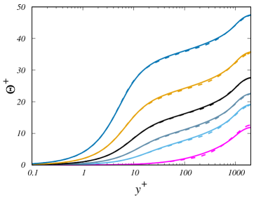
Figure 6: Comparison of mean temperature profiles obtained from DNS (solid lines) with the prediction of the compound fitting function given by (5) and (10), with fitting parameters listed in table 1 (dashed lines), for channel flow with symmetric heating (a) and with asymmetric heating (b), at $\mbox{{Re}}_{\tau}=1002$. The circles depicted in panel (b) represent the empirical predictions put forth by Kader [4]. Colour codes are as in table 3.

Application of the patching procedure outlined in §2.3 yields the temperature profiles depicted in figure 6. In the case of symmetric heating (left), deviations from a logarithmic behavior are small, and the compound temperature law fits well the DNS up to the channel centreline. Deviations from the logarithmic behavior are on the other hand quite strong in the case of asymmetric heating. Again, the agreement with the DNS data is quite good, with observable deviations limited to the lowest Prandtl number case. The correlation provided by Kader [4] also demonstrates reasonable performance in this scenario. However, it exhibits unnatural behavior in the buffer layer and tends to overpredict the strength of the wake.

4 Conclusions

We have presented fully explicit approximations for the mean temperature (or concentration) profiles for forced convection in internal flows. The model relies on universality of the inner-scaled mean temperature profile in the inner wall layer with respect to Reynolds number variations, and universality of the mean defect temperature profile in the core layer with respect to both Reynolds and Prandtl variations. The explicit representation of the temperature profile (5) is used for the inner layer, which effectively incorporates effects from Prandtl number variation. A simple quadratic profile (10) is then used for the core temperature profile, which includes a single flow-adjustable constant, which accounts for geometric and/or thermal forcing effects of the temperature field away from the wall. A patching condition is derived which guarantees smooth transition between the inner and the core layer. Comparison with the DNS results shows excellent predictive capability of the model, in a wide range of Prandtl numbers, deviations becoming visible only at $\mbox{{Pr}}\lesssim 0.1$. As for the effects of Reynolds number variation, we find that the model predictions are accurate as long as a sensible logarithmic layer is present, which occurs when $\mbox{{Pe}}_{\tau}=\mbox{{Pr}}\,\mbox{{Re}}_{\tau}\gtrsim 11$ [14]. We find that the present model constitutes a significant improvement over previous models developed for the prediction of the mean temperature distributions [4], as it yields much more realistic distributions within the wall layer as well as more accurate prediction of the shift of the log law with the Prandtl number. Given its modularity, the model lends itself to straightforward extension to cases with different flow geometry (e.g. boundary layers), and/or different heating conditions.

Acknowledgements
We acknowledge that the results reported in this paper have been achieved using the EuroHPC Research Infrastructure resource LEONARDO based at CINECA, Casalecchio di Reno, Italy, under a LEAP grant.

References

- Monin and Yaglom [1971] A. Monin, A. Yaglom, Statistical fluid mechanics: mechanics of turbulence, volume 1, MIT Press, Cambridge MA, 1971.
- Cebeci and Bradshaw [1984] T. Cebeci, P. Bradshaw, Physical and computational aspects of convective heat transfer, Springer-Verlag, New York, NY, 1984.
- Gowen and Smith [1967] R. Gowen, J. Smith, The effect of the Prandtl number on temperature profiles for heat transfer in turbulent pipe flow, Chem. Eng. Science 22 (1967) 1701–1711.
- Kader [1981] B. Kader, Temperature and concentration profiles in fully turbulent boundary layers, Int. J. Heat Mass Transfer 24 (1981) 1541–1544.
- Subramanian and Antonia [1981] C. Subramanian, R. Antonia, Effect of Reynolds number on a slightly heated turbulent boundary layer, Int. J. Heat Mass Transfer 24 (1981) 1833–1846.
- Nagano and Tagawa [1988] Y. Nagano, M. Tagawa, Statistical characteristics of wall turbulence with a passive scalar, J. Fluid Mech. 196 (1988) 157–185.
- Kim et al. [1987] J. Kim, P. Moin, R. Moser, Turbulence statistics in fully developed channel flow at low Reynolds number, J. Fluid Mech. 177 (1987) 133–166.
- Abe and Antonia [2009] H. Abe, R. Antonia, Near-wall similarity between velocity and scalar fluctuations in a turbulent channel flow, Phys. Fluids 21 (2009) 025109.
- Antonia et al. [2009] R. Antonia, H. Abe, H. Kawamura, Analogy between velocity and scalar fields in a turbulent channel flow, J. Fluid Mech. 628 (2009) 241–268.
- Levich [1962] V. Levich, Physicochemical Hydrodynamics, Prentice Hall, Englewood Cliffs. N.J., 1962.
- Kader and Yaglom [1972] B. Kader, A. Yaglom, Heat and mass transfer laws for fully turbulent wall flows, Int. J. Heat Mass Trans. 15 (1972) 2329–2351.
- Dittus and Boelter [1933] F. Dittus, L. Boelter, Heat transfer in automobile radiators of the tubular type, International Communications in Heat and Mass Transfer 12 (1933) 3–22.
- Kays et al. [1980] W. Kays, M. Crawford, B. Weigand, Convective heat and mass transfer, McGraw-Hill, 1980.
- Pirozzoli [2023a] S. Pirozzoli, Prandtl number effects on passive scalars in turbulent pipe flow, J. Fluid Mech. 965 (2023a) A7.
- Pirozzoli [2023b] S. Pirozzoli, An explicit representation for mean profiles and fluxes in forced passive scalar convection, J. Fluid Mech. 968 (2023b) R1.
- Musker [1979] A. Musker, Explicit expression for the smooth wall velocity distribution in a turbulent boundary layer, AIAA J. 17 (1979) 655–657.
- Pirozzoli et al. [2022] S. Pirozzoli, J. Romero, M. Fatica, R. Verzicco, P. Orlandi, DNS of passive scalars in turbulent pipe flow, J. Fluid Mech. 940 (2022) A45.
- Pirozzoli et al. [2016] S. Pirozzoli, M. Bernardini, P. Orlandi, Passive scalars in turbulent channel flow at high Reynolds number, J. Fluid Mech. 788 (2016) 614–639.
- Pirozzoli et al. [2021] S. Pirozzoli, J. Romero, M. Fatica, R. Verzicco, P. Orlandi, One-point statistics for turbulent pipe flow up to Re, J. Fluid Mech. 926 (2021) A28.
- Clauser [1956] F. Clauser, The turbulent boundary layer, Adv. Appl. Mech. 4 (1956) 1–51.
- Kawamura et al. [1999] H. Kawamura, H. Abe, Y. Matsuo, DNS of turbulent heat transfer in channel flow with respect to Reynolds and Prandtl number effects, Int. J. Heat Fluid Flow 20 (1999) 196–207.
- Abe et al. [2004] H. Abe, H. Kawamura, Y. Matsuo, Surface heat-flux fluctuations in a turbulent channel flow up to Re with Pr and , Int. J. Heat Fluid Flow 25 (2004) 404–419.
- Alcántara-Ávila et al. [2021] F. Alcántara-Ávila, S. Hoyas, M. Pérez-Quiles, Direct numerical simulation of thermal channel flow for Re= 5000 and Pr=0.71, J. Fluid Mech. 916 (2021) A29.
- Pirozzoli and Modesti [2023] S. Pirozzoli, D. Modesti, Direct numerical simulation of one-sided forced thermal convection in plane channels, J. Fluid Mech. 957 (2023) A31.
- Balasubramanian et al. [2023] A. Balasubramanian, L. Guastoni, P. Schlatter, R. Vinuesa, Direct numerical simulation of a zero-pressure-gradient turbulent boundary layer with passive scalars up to prandtl number Pr = 6, J. Fluid Mech. 974 (2023) A49.