50pt40pt0pt60pt

Assessing the similarity of real matrices with arbitrary shape

Jasper Albers^1,2*†, Anno C. Kurth^1,2*†, Robin Gutzen¹, Aitor Morales-Gregorio¹, Michael Denker¹, Sonja Grün^1,3,4, Sacha J. van Albada^1,5, Markus Diesmann^1,3,6,7

¹Institute for Advanced Simulation (IAS-6), Jülich Research Centre, Jülich, Germany. ²RWTH Aachen University, Aachen, Germany. ³JARA-Institut Brain Structure-Function Relationships (INM-10), Jülich Research Centre, Jülich, Germany. ⁴Theoretical Systems Neurobiology, RWTH Aachen University, Aachen, Germany. ⁵Institute of Zoology, University of Cologne, Cologne, Germany. ⁶Department of Psychiatry, Psychotherapy and Psychosomatics, School of Medicine, RWTH Aachen University, Aachen, Germany. ⁷Department of Physics, Faculty 1, RWTH Aachen University, Aachen, Germany.
^*These authors contributed equally to this work.
^† j.albers@fz-juelich.de, a.kurth@fz-juelich.de
Assessing the similarity of matrices is valuable for analyzing the extent to which data sets exhibit common features in tasks such as data clustering, dimensionality reduction, pattern recognition, group comparison, and graph analysis. Methods proposed for comparing vectors, such as cosine similarity, can be readily generalized to matrices. However, this approach usually neglects the inherent two-dimensional structure of matrices. Here, we propose singular angle similarity (SAS), a measure for evaluating the structural similarity between two arbitrary, real matrices of the same shape based on singular value decomposition. After introducing the measure, we compare SAS with standard measures for matrix comparison and show that only SAS captures the two-dimensional structure of matrices. Further, we characterize the behavior of SAS in the presence of noise and as a function of matrix dimensionality. Finally, we apply SAS to two use cases: square non-symmetric matrices of probabilistic network connectivity, and non-square matrices representing neural brain activity. For synthetic data of network connectivity, SAS matches intuitive expectations and allows for a robust assessment of similarities and differences. For experimental data of brain activity, SAS captures differences in the structure of high-dimensional responses to different stimuli. We conclude that SAS is a suitable measure for quantifying the shared structure of matrices with arbitrary shape.

Keywords: matrix comparison, singular value decomposition, networks, brain activity analysis

1 Introduction

Social groups, transportation systems, chemical reactions, brains - many complex systems are governed and commonly characterized by the pairwise interactions of their constituent elements. Typically, these interactions are described by matrices that can represent covariance structures, spatio-temporal dependencies, or the connections and interactions in a network, forming the foundation for the mathematical treatment of such complex systems [1]. Common examples include genetic variance [2], ecological food chains [3], or stock markets [4]. Additionally, many other types of structured data can be represented in matrix form, ranging from test scores for groups of subjects to parallel time series data. Quantifying the similarity between such matrices is important for distinguishing features of the underlying systems.

Conventional measures of the similarity between two matrices $A$ and $B$ are often based on the Frobenius scalar product $\langle A,B\rangle_{F}=\mathrm{tr}(AB^{T})$, leading to the Frobenius norm $||A-B||^{2}_{F}~{}=~{}\langle A-B,A-B\rangle_{F}$, or the cosine similarity $\langle A,B\rangle_{F}$ where $||A||_{F}=||B||_{F}=1$ [5, 6]. However, the Frobenius norm and cosine similarity only take into account the numerical values of corresponding entries of the matrices and ignore their two-dimensional structure.

Another more involved approach reformulates ideas borrowed from canonical correlation analysis (CCA)[7] in the context of the comparison of two matrices [8]. It relies on the canonical angles between the subspaces spanned by the columns of the matrices. Here, problems may arise if the embedding space (the number of rows) is of similar size as the number of columns and, at the same time, the subspaces spanned by these columns are high-dimensional (relative to the dimension of the embedding space). In this case, the canonical angles cannot meaningfully distinguish the subspaces, limiting the applicability of this approach.

Previous work addresses the comparison of symmetric matrices using eigenangles—the angles between eigenvectors of the compared matrices [9]. Small eigenangles indicate a good alignment of the respective eigenspaces, enabling the definition of a similarity score. The authors employ an analytical description of the similarity score based on random matrix theory to devise a statistical test for the comparison of such matrices. Asymmetric matrices usually have complex eigenvectors and eigenvalues, making their ordering ambiguous. Thus, an extension of the eigenangle test to asymmetric matrices is not straightforward. Furthermore, the eigenangle test is by definition not applicable to non-square matrices. In this study, we overcome both limitations by proposing a refined matrix similarity measure that naturally extends to the comparison of any two real matrices with identical shapes. Using singular value decomposition (SVD) instead of eigendecomposition, we derive SAS from the respective left and right singular vectors and singular values.

In Section 2, we formally define SAS and derive basic properties. Further, three types of matrices are introduced that we use in the following for the evaluation of SAS and comparison to other similarity measures: random matrices with continuously distributed entries (Section 2.2), adjacency matrices of random graphs (Section 2.3), and massively parallel neural activity recordings (Section 2.4).

We start our analysis (Section 3) by providing a geometric interpretation of SAS. Next, we compare SAS with standard similarity measures for matrices: on the basis of generic random matrices we show that only SAS captures certain salient two-dimensional correlation structures. Third, we characterize the behavior of SAS under changes in dimensionality and perturbation of entries. Fourth, we evaluate the similarity across instances of six probabilistic graph models that are commonly used to describe network architecture. With this use case, we demonstrate that SAS is able to differentiate between the connectivity in network graphs by means of their adjacency matrices. Finally, we apply SAS on experimental data, evaluating the similarity of brain activity in the visual cortex of macaques in response to four different visual stimuli. This application shows that SAS can identify underlying features in the presence of realistic noise.

In conclusion (Section 4), we show that SAS is a well-behaved measure for structural similarity in matrices that is applicable in different scientific domains. It highlights shared variability between matrices and allows for a distinction of models or processes underlying their generation.

2 Methods

2.1 Singular angle similarity

To assess the similarity of two arbitrary, real, $m\times n$ matrices $M_{a},M_{b}$, we devise a measure based on singular value decomposition (SVD) [10]. Without loss of generality, we assume $m\leq n$. SVD guarantees the existence of orthogonal matrices $U_{i}\in\mathbb{R}^{m\times m}$ and $V_{i}\in\mathbb{R}^{n\times n}$, and diagonal matrices $\Sigma_{i}=\mathrm{diag}(\sigma_{i}^{1},...,\sigma_{i}^{m})\in\mathbb{R}^{m\times n}$ where $\sigma_{i}^{j}\geq\sigma_{i}^{l}\geq 0$ for $l>j\geq 1$ such that

$$M_{i}=U_{i}\Sigma_{i}V_{i}^{T}~{}.$$ (1)

Here, $i\in\{a,b\}$. SVD is schematically presented for a $2\times 2$ case in Figure 1. The columns of $V_{i}$, denoted by $v_{i}^{1},...,v_{i}^{n}$, are the right singular vectors, and the columns of $U_{i}$, denoted by $u_{i}^{1},...,u_{i}^{m}$, are the left singular vectors. With this, the SVD can also be written in the form

$$M_{i}=\sum_{j=1}^{m}\sigma_{i}^{j}u_{i}^{j}\otimes v_{i}^{j}~{}.$$ (2)

Here, $\otimes$ denotes the outer product of two vectors. Thus, under the action of $M_{i}$ the vectors $v^{j}_{i}$ are transformed into the vectors $\sigma_{i}^{j}u_{i}^{j}$. The singular values $\sigma_{i}^{1},...,\sigma_{i}^{m}$ are unique—they are the square root of the eigenvalues of $M_{i}M_{i}^{T}\in\mathbb{R}^{m\times m}$. Left and right singular vectors that correspond to non-degenerate singular values are uniquely determined up to a joint multiplication by $-1$. Thus, the vector pairs $(u_{i}^{j},v_{i}^{j})$ and $(-u_{i}^{j},-v_{i}^{j})$ both are equally valid singular vectors to a non-degenerate singular value $\sigma_{i}^{j}\geq 0$. Singular vectors associated with degenerate singular values are unique up to an action of an orthogonal transformation on the subspace spanned by these singular vectors. In the following, we assume that there are no degenerate singular values except zero. For the overwhelming majority of higher-dimensional matrices encountered in practice, this assumption is satisfied.
We note that if both $M_{i}$ are symmetric positive-definite matrices (e.g., covariance matrices), then $U_{i}=V_{i}$, and the singular values become the eigenvalues.
If $\min\{\sigma_{a}^{j},\sigma_{b}^{j}\}\neq 0$ we define the left singular angle $\alpha^{j}(U)$ and the right singular angle $\alpha^{j}(V)$ of the first kind as

$$\alpha^{j}(U) =\sphericalangle(u_{a}^{j},u_{b}^{j})=\arccos\left(\langle u_{a}^{j},u_{b}^{j}\rangle\right),$$

$$\quad\alpha^{j}(V) =\sphericalangle(v_{a}^{j},v_{b}^{j})=\arccos\left(\langle v_{a}^{j},v_{b}^{j}\rangle\right).$$ (3)

Due to the ambiguity in vector pairs of left and right singular vectors we additionally define left singular angles of the second kind as $\alpha^{j}(U^{-})=\sphericalangle(-u_{1}^{j},u_{2}^{j})=\sphericalangle(u_{1}^{j},-u_{2}^{j})$ and mutatis mutandis for right singular angles of the second kind $\alpha^{j}(V^{-})$. The singular angles of the first and second kinds are visualized in Figure 1.

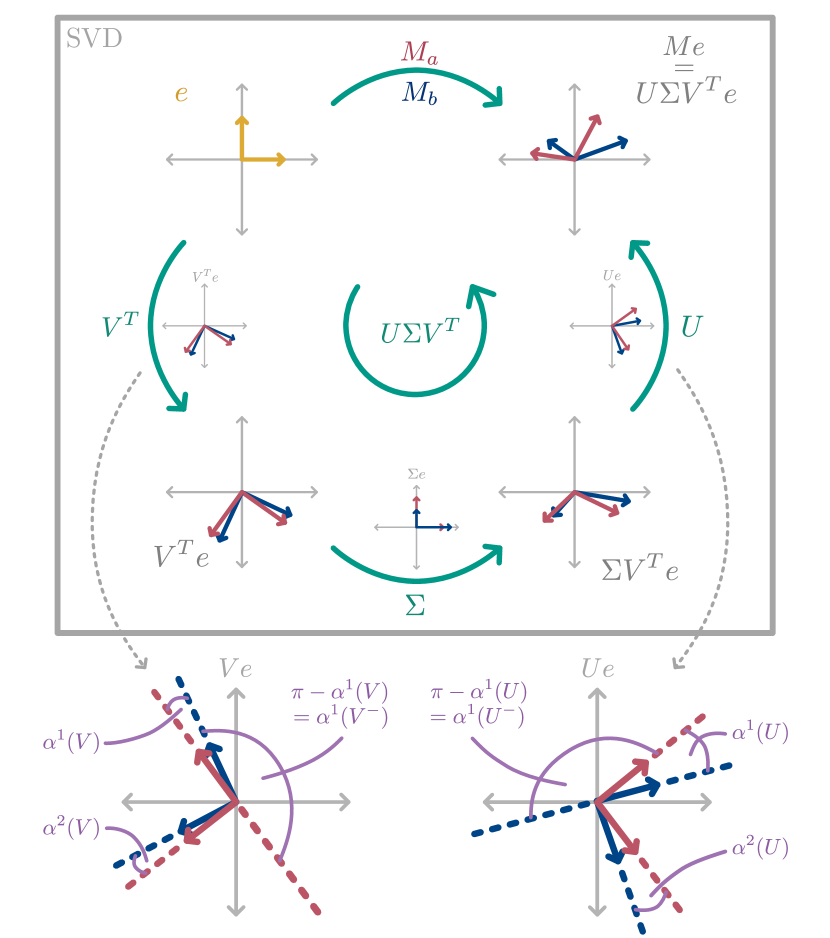
Figure 1: Singular value decomposition. Schematic representation of the transformations applied on the basis vectors $e$ (yellow) by the components of SVD for two $2\times 2$ matrices $M_{a}$ (red) and $M_{b}$ (blue). Small graphs next to the green arrows illustrate the isolated action of the corresponding transformations $V^{T}$, $\Sigma$, and $U$ on $e$. Below, the singular angles of the first ($\alpha^{j}(V)$ and $\alpha^{j}(U)$) and second ($\alpha^{j}(V^{-})$ and $\alpha^{j}(U^{-})$) kinds are shown as the angles between the column vectors of $V_{a}$ and $V_{b}$, and $U_{a}$ and $U_{b}$, respectively, as defined in Equation 3.

From Figure 1 we have

$$\alpha^{j}(U)+\alpha^{j}(U^{-})=\pi=\alpha^{j}(V)+\alpha^{j}(V^{-})~{}.$$ (4)

Due to the ambiguity in the sign, one has to consider either $\left(\alpha^{j}(U),\alpha^{j}(V)\right)$ or $\left(\alpha^{j}(U^{-}),\alpha^{j}(V^{-})\right)$ together. We define the singular angle as the smaller average of the two choices

$$\alpha^{j} =\min\left\{\frac{\alpha^{j}(U)+\alpha^{j}(V)}{2},\frac{\alpha^{j}(U^{-})+\alpha^{j}(V^{-})}{2}\right\}$$

$$=\min\{\bar{\alpha}^{j},\pi-\bar{\alpha}^{j}\}$$ (5)

where $\bar{\alpha}^{j}=(\alpha^{j}(U)+\alpha^{j}(V))/2$. Using the angular similarity

$$\Delta^{j}=1-\frac{\alpha^{j}}{\pi/2}\in[0,1]$$ (6)

and defining the singular value score as $w^{j}=w(\sigma_{a}^{j},\sigma_{b}^{j})$ where $w(x,y)\geq 0$ denotes a weight function, we calculate SAS as the weighted average of the angular similarities:

$$\mathrm{SAS}=\frac{\sum_{j}^{k}w^{j}\Delta^{j}}{\sum_{j}^{k}w^{j}}\in[0,1]~{}.$$ (7)

Here, $k$ is the largest natural number less than or equal to $m$ such that $\min\{\sigma^{k}_{a},\sigma^{k}_{b}\}\neq 0$. In the following, we choose

$$w(x,y)=(x+y)/2~{}.$$ (8)

Another possible choice is $w(x,y)~{}=~{}\sqrt{(x^{2}~{}+~{}y^{2})/2}$ (c.f. [9]). One can substitute other vector-based similarity measures for the angular similarity defined in Equation 6. For example, substituting cosine similarity yields $\Delta^{j}~{}=~{}\cos(\alpha^{j})$.

According to our definition of SAS in Equation 7, singular angles stemming from singular vectors of which at least one has a corresponding singular value of zero do not contribute to SAS. In the rare case that a singular value is degenerate, the canonical angles between the subspaces spanned by the corresponding singular vectors can be used in the calculation of SAS. Further, when calculating SAS, $\alpha^{j}(V)$ for $j>m$ are not used even though they are well-defined. This is because the corresponding right singular vectors do not contribute to the transformation given by $M_{i}$. Indeed, writing $e^{j}$ for the $j$-th standard unit vector, we have

$$M_{i}v_{i}^{j}=U_{i}\Sigma_{i}V_{i}^{T}v_{i}^{j}=U_{i}\Sigma e^{j}~{}.$$

As $\Sigma e^{j}=0$ if $j>m$, right singular vectors $v_{i}^{j}$ satisfying this constraint are discarded since $v_{i}^{j}\in\ker M_{i}$.

In SAS, singular vectors of different matrices are compared based on the ordering of the singular values. If two singular values are close, small perturbations can lead to a change in their order and therefore change which vectors are compared, potentially leading to different SAS values. Alternatively, other criteria could be used for pairing the singular vectors between which the singular angles are calculated. For example, one could sequentially pair vectors that enclose the smallest angle, thereby calculating the difference in alignment between the subspaces spanned by the singular vectors. See Section S1.1 for a derivation and discussion of this alternative measure.

2.2 Random matrices

To compare SAS to standard measures of matrix similarity, we define the following classes of random matrices with shape $N\times N$ where each entry is drawn from a continuous probability distribution. Numerical values for the corresponding model parameters are summarized in Table 1.

Uncorrelated normal matrix (UC)

For random matrices of this class, each entry is drawn independently from a normal distribution with the same mean $\mu$ and variance $\sigma^{2}$. Collections of these matrices are also referred to as real Ginibre Ensembles.

Cross-correlated normal matrix (CC)

We first independently sample $N$ random vectors from an $N$-dimensional normal distribution with mean $\mu$ and covariance matrix $C$ where

$$C_{ij}=\frac{a}{N}\cdot\exp\left(-b\frac{|i-j|}{N}\right)~{}.$$

Thus, the entries of the correlation matrix decay exponentially with distance from the diagonal. The sampled vectors are the columns of an $N\times N$ matrix $K^{1}$. We repeat the process to obtain an independent matrix $K^{2}$ to finally define $K=(K^{1}+{K^{2}}^{T})/2$. Since each entry of the $K^{i}$ is normally distributed, so is each entry of their sum $K$, and the covariance between entries $K_{kl}$ and $K_{mn}$ is $(C_{kl}+C_{mn})/4$. Normalization by $N$ in the argument of the exponential ensures that the strength of the correlation scales with the size of the matrix.

Cross-correlated block matrix (CB)

Again, uncorrelated normal (UC) matrices $B$ are sampled. Then, the entries $B_{kl}$ where $k^{\mathrm{lower}}\leq k\leq k^{\mathrm{upper}}$ and $l^{\mathrm{lower}}\leq l\leq l^{\mathrm{upper}}$ are replaced by a correlated normal structure as defined above.

Shuffled, cross-correlated block matrix (SB)

Matrices are sampled according to CB. Then, the rows are permuted randomly while the columns remain untouched.

Parameter	Model(s)	Meaning	Value
$N$	all	dimensionality	$300$
$\mu$	all	mean of distribution	$0$
$\sigma^{2}$	UC	variance of distribution	$1/N$
$a$	CC	peak covariance	$10$
$b$	CC	inverse characteristic length	$100$
$k^{\mathrm{lower}}$	CB	block coordinate	$10$
$k^{\mathrm{upper}}$	CB	block coordinate	$90$
$l^{\mathrm{lower}}$	CB	block coordinate	$10$
$l^{\mathrm{upper}}$	CB	block coordinate	$90$

Table 1: Parameters of random matrices: uncorrelated normal matrix (UC), cross-correlated normal matrix (CC), cross-correlated block matrix (CB), and shuffled, cross-correlated block matrix (SB).

2.3 Random graphs

We compare the adjacency matrices of six well-known network models with SAS. For all graphs, we derive the parameters such that the mean total number of connections $N_{c}$ in the graph is conserved. Table 2 summarizes the numerical values chosen for the corresponding model parameters.

Erdős-Rényi (ER)

In this network model [11], every connection has the same probability of being realized: $p~{}=~{}\frac{N_{c}}{N_{e}}$, where $N_{e}$ is the total number of possible connections in the graph. Note that this network model maximizes the entropy under the constraint that the mean number of connections is fixed [12].

Directed configuration model (DCM)

In a directed configuration model [13], a two-step probabilistic process is applied. First, random indegrees and outdegrees are drawn for each node such that the total number of connections across nodes is preserved (we fix these numbers for all graph instances). Second, connections are established by randomly matching each outgoing connection with an incoming connection. Thus, two nodes can have more than one connection, and the resulting adjacency matrix is not strictly binary.

One-cluster Erdős-Rényi (OC)

Based on an Erdős-Rényi (ER) graph, we introduce a single cluster by increasing $p$ between a certain subset of nodes of the network, while uniformly decreasing $p$ for all other connections such that $N_{c}$ is conserved. The relative increase of $p$ denoted by $r$, the cluster size denoted by $s$, and the location of the cluster defined by $k^{\mathrm{lower}},k^{\mathrm{upper}}$ and $l^{\mathrm{lower}},l^{\mathrm{upper}}$ are free parameters of this model.

Two-cluster Erdős-Rényi (TC)

For the two-cluster ER network, we create two non-overlapping clusters using the same method as in the OC model. Apart from the cluster sizes $s_{1}$ and $s_{2}$, the same parameters are used. The nodes that form the clusters are chosen such that there is maximal overlap with the single cluster of the OC model.

Watts-Strogatz (WS)

We create a small-world network following [14]. Here, $N_{n}$ nodes initially form a ring, where each node is connected to $k=\frac{N_{c}}{N_{e}}(N_{n}-1)$ of its nearest neighbors. Afterwards, all connections are uniformly redistributed with probability $p_{WS}$. Note that this model is undirected.

Barabási-Albert (BA)

As an example of a scale-free network, we create Barabási-Albert networks as introduced in [15]. Here, from an initial star graph with $m=\frac{N_{c}}{N_{e}}(N_{n}-1)/2$ nodes, new nodes are added subsequently until the desired number of nodes $N_{n}$ is reached. Each added node is connected to $m$ existing nodes, where the probability of each existing node being selected for a new connection is proportional to the number of connections it already has. Note that this model is undirected.

Param.	Model(s)	Meaning	Value
$N_{n}$	all	number of nodes	$300$
$N_{e}$	all	number of possible connections	$90000$
$N_{c}$	all	mean number of connections	$9000$
$r$	OC	relative increase of $p$ in cluster	$10$
$s$	OC	cluster size	$50$
$k^{\mathrm{lower}}$	OC	cluster coordinate	$50$
$k^{\mathrm{upper}}$	OC	cluster coordinate	$100$
$l^{\mathrm{lower}}$	OC	cluster coordinate	$50$
$l^{\mathrm{upper}}$	OC	cluster coordinate	$100$
$s_{1}$	TC	size of cluster 1	$40$
$s_{2}$	TC	size of cluster 2	$10$
$p_{\mathrm{WS}}$	WS	reconnection probability	$0.3$

Table 2: Parameters of random graphs: Erdős-Rényi (ER), directed configuration model (DCM), one cluster (OC), two clusters (TC), Watts-Strogatz (WS), and Barabási-Albert (BA).

2.4 Brain data

We apply SAS to compare non-square matrices of brain activity in response to visual stimuli. We use an openly available data set, which has an extensive description of the task and recording apparatus [16]. In the experiments, the activity of neurons in the primary visual cortex (V1) of one macaque monkey (Macaca mulatta) was recorded using several extracellular electrode arrays (Utah arrays, $8\times 8$ electrodes). The quality of the signals was assessed based on the signal-to-noise ratio and channel impedance. For details of the data recording and processing we refer to [16]. Here, we focus on a single array ($\rm ID=11$) during a receptive field mapping task. In this task, for each trial the macaque had to fixate its gaze to the center of the screen for $\rm 200~{}ms$. Subsequently, one bright bar moved across the screen for $\rm 1000~{}ms$ in one of four directions: rightward (R), leftward (L), upward (U), or downward (D). The different task modalities are in the following referred to as trial types. For each trial type, there are $N=120$ repetitions.

The activity time series recorded from the electrodes was processed to obtain the multi-unit activity envelope (MUAe) with a sampling rate of $\rm 1~{}kHz$, a commonly used signal as a proxy for neuronal firing rates [17], see [18] for specific details of the processing. We align the trials to the peak response, defined as the maximum response from the average MUAe across electrodes, and cut data in a window $\rm\pm 200~{}ms$ around the alignment trigger. This yields one $\rm 64\times 400$ matrix per trial: $64$ electrodes during $\rm 400~{}ms$ at $\rm 1~{}kHz$; see examples in Figure 6B. We then group the matrices by trial type for comparison by SAS.

3 Results

We present a measure for assessing the structural similarity between two arbitrary, real $m\times n$ matrices $M_{a},M_{b}$ named singular angle similarity (SAS). The measure is based on singular value decomposition (SVD), which introduces the left and right singular vectors with corresponding singular values (Equation 1). SAS exhibits the following properties:

• SAS attains values between $0$ and $1$ where higher values imply greater similarity.

• SAS is invariant under actions of identical orthogonal maps from the left or the right on the compared matrices; this includes the consistent permutation of rows and columns as a special case (Section S1.2).

• SAS is invariant under transposition of both matrices (Section S1.2).

• SAS is invariant under scaling with a positive factor; in particular, SAS $=1$ for $M_{b}=c_{1}M_{a},c_{1}\in\mathbb{R}^{+}$ (Section S1.3).

• SAS is zero if the two compared matrices are equal up to a negative factor: $\mathrm{SAS}~{}=~{}0$ for $M_{b}=c_{2}M_{a},c_{2}\in\mathbb{R}^{-}$ (Section S1.3).

Thus, SAS predominantly highlights structural differences between the matrices. The derivation of this measure is presented in Section 2.1.

3.1 Geometric interpretation of SAS

Singular angle similarity has a geometric interpretation. The left and right singular vectors of $M_{i}$ ($i\in\{a,b\}$) are the respective eigenvectors of the square matrices $M_{i}M_{i}^{T}$ and $M_{i}^{T}M_{i}$. Further, $M_{i}M_{i}^{T}$ and $M_{i}^{T}M_{i}$ have the same eigenvalues (the squared singular values of $M_{i}$). Consider for each of these symmetric positive-definite matrices a hyperellipsoid spanned by the respective eigenvectors scaled by their eigenvalues (Figure 2).

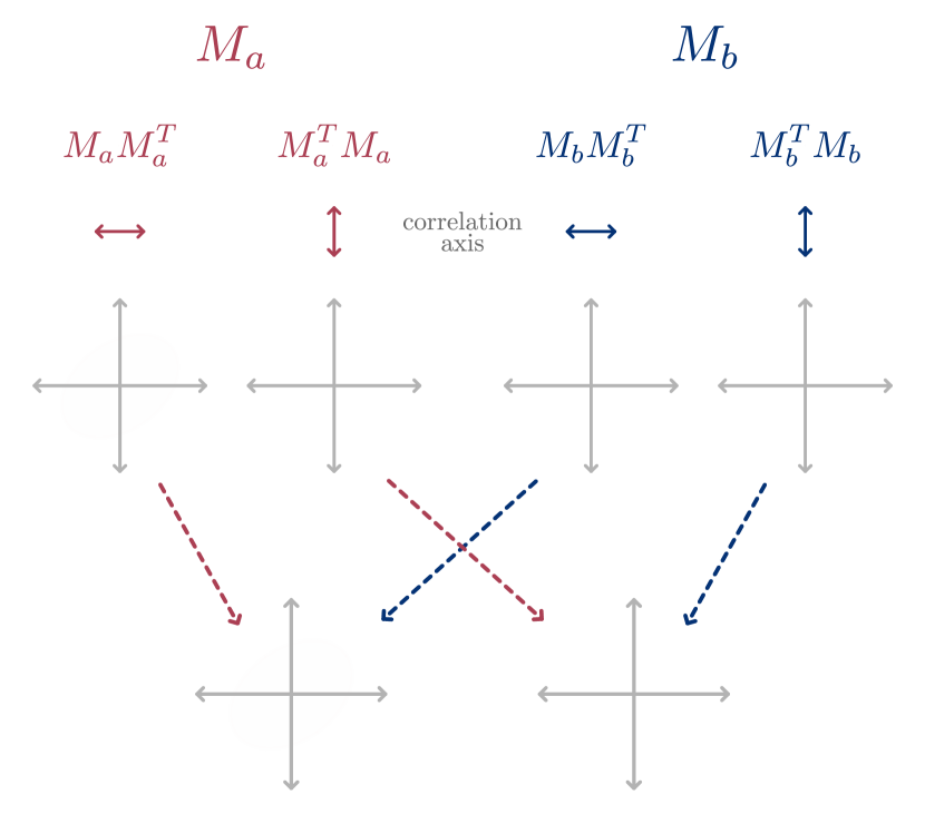
Figure 2: Geometric interpretation of SAS. Matrices $M_{a}$ (red) and $M_{b}$ (blue) as in Figure 1. The eigenvectors of $M_{i}M_{i}^{T}$ and $M_{i}^{T}M_{i}$ (same colors) scaled by the square root of their eigenvalues span the main axes of ellipsoids. These square matrices capture the correlation structure of $M_{i}$ along the horizontal and vertical axis, respectively (double-headed colored arrows). SAS compares the angles between the corresponding ellipsoids (dashed colored arrows).

The hyperellipsoid collapses in most dimensions as matrices $M_{i}$ typically have only a small number of large singular values (c.f. [19]). Dimensions associated with the largest singular values dominate its shape, and the angle between the corresponding left and right singular vectors of the matrices $M_{a}$ and $M_{b}$ are of main relevance for SAS. Thus, a high SAS indicates that the hyperellipsoids are aligned, whereas a low SAS indicates misalignment or different shapes. If two matrices share two-dimensional structural features, their hyperellipsoids will be similarly shaped and point into similar directions, producing a high SAS. $M_{i}M_{i}^{T}$ and $M_{i}^{T}M_{i}$ are the correlation matrices up to a normalization by the number of rows and columns, respectively, and the subtraction of the mean. Therefore, SAS takes into account the correlation structure along both axes of the matrices. This distinguishes the measure from common methods such as cosine similarity and the Frobenius norm.

3.2 Comparison with standard measures for random matrices

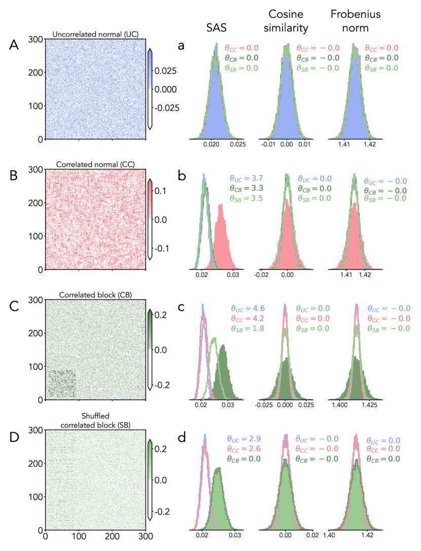
Figure 3: Comparison of SAS with standard measures. A–D Single instances of the different random matrix classes. For visibility, negative values are shown as white. a–d Histograms of SAS, cosine similarity, and the Frobenius norm between instances of the random matrix classes ($n=100$, all pairs compared). Filled distributions indicate self-similarities (self-distances), non-filled ones indicate cross-similarities (cross-distances). Legends show effect sizes $\theta$ for the comparison between distributions.

By its very definition, SAS captures two-dimensional structures that are invisible to traditional measures of matrix similarity. Figure 3 shows the ability of different measures to discriminate between classes of random matrices with such structure. Concretely, we compare SAS with cosine similarity,

$$\langle M_{a},M_{b}\rangle_{F}=\mathrm{tr}(M_{a}M_{b}^{T})~{},$$ (9)

and Frobenius distance,

$$||M_{a}-M_{b}||_{F}=\sqrt{\langle M_{a}-M_{b},M_{a}-M_{b}\rangle_{F}},$$ (10)

where we normalize the matrices such that

$$||M_{a}||_{F}~{}=||M_{b}||_{F}=1~{}.$$

Figure 3A–D show single instances of the four matrix classes defined in Section 2.2. We first calculate the self-similarity, the pairwise similarity between instances of the same random matrix class, and the cross-similarity, which refers to the similarity between instances of different classes (Figure 3a–d). We analogously define self- and cross-distance for the Frobenius distance. Subsequently, we investigate whether the different measures distinguish the random matrix classes from each other based on realizations of their particular structures. Fundamentally, this only works if the structure quantified by a measure is more similar between instances of the same class than across classes. Thus, for SAS and cosine similarity, the self-similarity must be meaningfully greater than the cross-similarities. Conversely, since the Frobenius norm measures a distance rather than a similarity, the self-distance must be smaller than the cross-distance. We call a difference meaningful if the effect size $\theta$ between pairs of distributions is greater than one. Assuming an underlying Gaussian model for the distributions, we employ the definition

$$\theta=\frac{\mu_{\mathrm{self}}-\mu_{\mathrm{cross}}}{\sqrt{\frac{\sigma_{\mathrm{self}}^{2}+\sigma_{\mathrm{cross}}^{2}}{2}}}$$ (11)

of the ”Cohen’s D” effect size [20] underlying the common Student’s and Welch’s t-statistics [21, 22], where $\mu$ and $\sigma$ are the mean and standard deviation of the self- and cross-similarity distributions. Thus, two distributions are meaningfully different if the distance of their means is greater than the quadratic mean of their standard deviations.

Figure 3a shows that UC matrices cannot be distinguished from the other matrix classes by any measure. This is expected: since the entries are independent, there is no detectable structure. In particular, this means that no structure is shared between different UC matrices or between UC matrices and matrices of other classes. Geometrically, this corresponds to ellipsoids that are oriented in random directions for each instance.

By definition, CC matrices exhibit such fluctuations. However, cosine similarity and the Frobenius norm fail to identify the common correlation structure (Figure 3b). Only SAS separates the self- and cross-similarity meaningfully and can thereby distinguish this matrix class from the others.

A similar conclusion holds true for CB matrices, where the correlated structure is embedded into an otherwise uncorrelated matrix (Figure 3c): again, only SAS separates the self- and cross-similarities meaningfully.

Finally, we consider SB matrices. By construction, these are CB matrices with permuted rows. Between SB matrices, the CB correlation structure along the horizontal axis (quantified by $MM^{T}$) is destroyed while the correlation structure along the vertical axis (quantified by $M^{T}M$) stays the same. Since SAS takes into account both, it detects similarity between SB and CB matrices despite the permutation of the rows. This leads to a higher cross-similarity between CB and SB matrices than between CB and the other matrix classes (Figure 3c). Since the block structure exhibited by CB matrices can be viewed as one specific permutation of the rows, the self-similarity of SB and the cross-similarity between SB and CB follow the same distribution (Figure 3d) while SB matrices are separable from UC and CC matrices. The cosine similarity and the Frobenius norm fail to separate SB matrices from the other classes. The choice of the axis along which we permute is arbitrary; the results are identical if we permute columns instead of rows.

Why are these examples relevant? They show that SAS captures certain two-dimensional correlation structures between instances. In contrast, the traditional measures cannot identify them. Additionally, SAS retains similarity even after permutation along one axis—including shifts as a special case. This is relevant in practical applications, for example in the analysis of highly parallel time series: even if the time series are not aligned, SAS exposes structural similarities.

3.3 Characterization of scale dependence and robustness

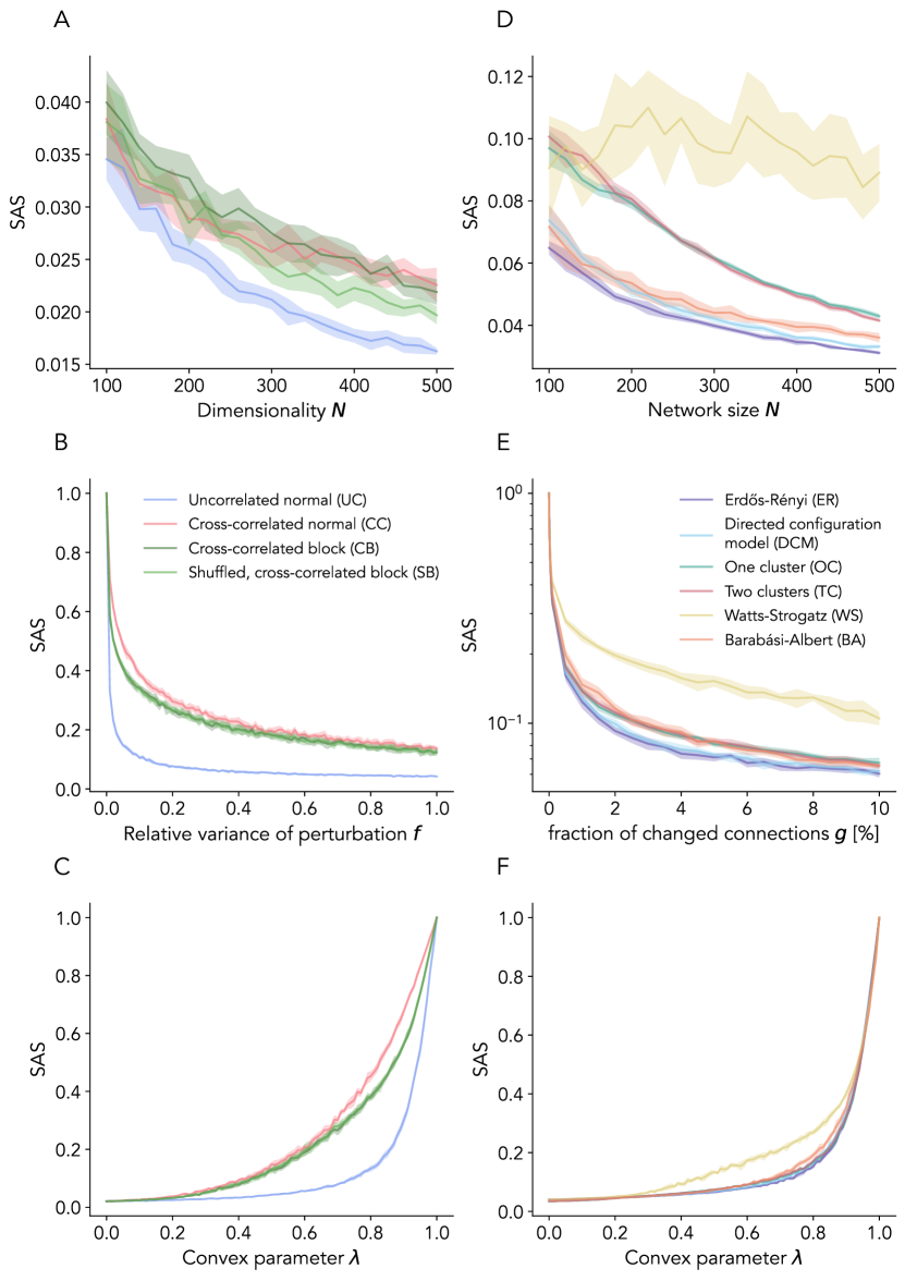
Figure 4: Characterization of singular angle similarity. In all panels, solid lines indicate the mean, the shading the standard deviation over 10 realizations. A SAS between instances of the same matrix class for varying dimensionality $N$. B SAS between identical matrix instances under varying variance of an additive perturbation with $\sigma^{2}_{\mathrm{pert}}=f\sigma^{2}$. Matrices are of dimensionality $N=300$. C SAS between matrices when increasing the degree of putative structural similarity quantified by $\lambda$. D SAS between instances of the same network model for varying network size $N$. E SAS between identical network model instances where the number of individual connections that are changed is gradually increased. Networks are of size $N=300$. F SAS between network model instances when increasing the degree of putative structural similarity quantified by $\lambda$.

To assess the dependence of SAS on matrix size, we calculate the self-similarity for increasing dimensionality $N$ and observe a decreasing SAS for all random matrix classes (Figure 4A). Since the probability distribution for an angle between two random vectors increasingly centers around $\pi/2$ with increasing dimensionality [23], the resulting SAS between UC matrices decreases with increasing matrix dimensionality. This intuition generalizes to the other matrix classes. Hence, a quantitative comparison of SAS values is only reasonable for matrices of the same dimensionality.

Next, we investigate how SAS decreases between two identical copies of a matrix when gradually perturbing one of them. We analytically study SAS between a matrix $M$ and a perturbed version of itself, $M+\sqrt{\epsilon}W$, using Rayleigh-Schrödinger perturbation theory [24]. Here, $\sqrt{\epsilon}$ is chosen as a perturbation parameter since this ensures a linear scaling of the variance of the perturbation matrix with $\epsilon$. We find that, for a large class of perturbations, SAS follows $1-\arccos\left(1-O(\epsilon)\right)/\frac{\pi}{2}$ (see Section S1.4). This implies that small differences are identified as dissimilarities arbitrarily fast ($\frac{d\arccos(1-x)}{dx}~{}\rightarrow~{}\infty$ for $x~{}\rightarrow~{}0$). Thus, SAS is sensitive to small differences in the compared matrices. For an empirical analysis, we study the sensitivity of SAS under perturbations of the form $\tilde{M}=M+W$ where $W$ is a matrix of the UC class with zero mean and variance $\sigma^{2}_{\mathrm{pert}}=f\sigma^{2}$, $0\leq f\leq 1$. As predicted analytically, Figure 4B shows a rapid fall-off for small perturbations that continues as a gradual decrease for each of the considered classes.

Finally, we numerically study SAS while adding structure to a noise matrix. In particular, we calculate SAS between a matrix $M$ and the convex combination of the same matrix with a UC matrix $N$:

$$(1-\lambda)N+\lambda M\qquad\textnormal{for }\lambda\in[0,1]~{}.$$ (12)

Figure 4C shows that SAS is well-behaved also for small values of $\lambda$: it increases smoothly when adding structure for all matrix classes.

We perform an analogous analysis for network adjacency matrices of six different graph models: Erdős-Rényi (ER), directed configuration model (DCM), one cluster (OC), two clusters (TC), Watts-Strogatz (WS), and Barabási-Albert (BA), as defined in Section 2.3. The results are qualitatively similar to those obtained for the four classes of random matrices: SAS decreases with increasing network size $N$ (Figure 4D), SAS rapidly decreases for small perturbations (Figure 4E), and SAS gradually increases when adding structure (Figure 4F). A notable exception is that for WS networks, SAS does not decrease when increasing $N$. In this network model the number of nearest neighbors each node is connected to scales with $N$. Therefore the correlation in the adjacency matrix also scales with $N$, rendering the similarity measured by SAS independent of $N$. For investigating the effect of a perturbation on identical network matrices (Figure 4E), we define the gradual change such that an increasing fraction $g$ of matrix elements is altered. Specifically, for each of the $gN^{2}$ randomly selected matrix elements, existing connections are removed and missing connections are established with a multiplicity of one. For the binary adjacency matrices this corresponds to bit-flipping the corresponding entries. In the case of adding structure (Figure 4F), we choose the ER adjacency matrices as the noise component $N$. Note that while the sum over all entries stay the same on average under the convex combination, the entries are not confined to natural numbers anymore.

3.4 Categorization of random graphs

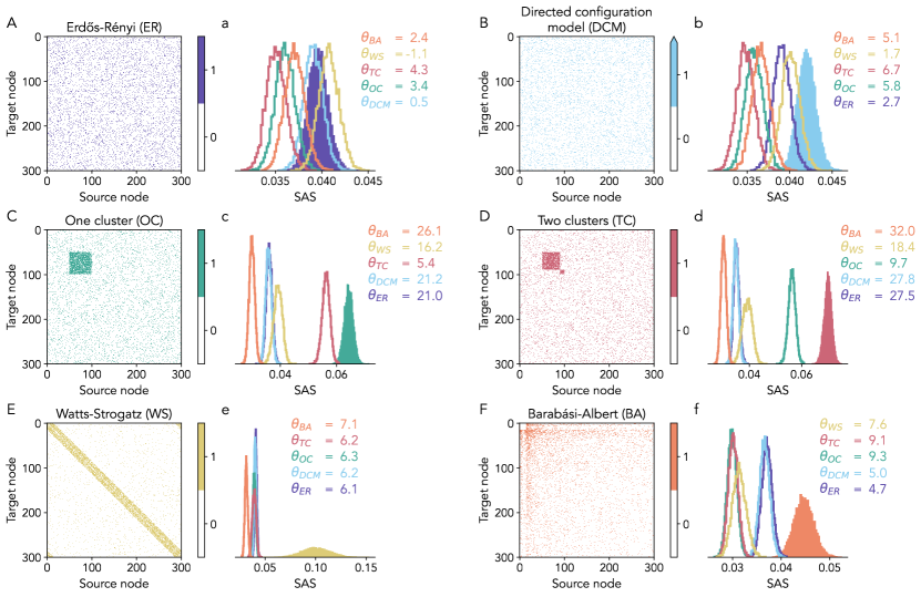
Figure 5: Self- and cross-similarity of different network models. A–F Single instances of the different network models. Colored matrix elements indicate a connection between nodes. For the DCM model, connections with a multiplicity higher than one are shown with the same color intensity as single connections. a–f Histograms of SAS between instances of the network models ($n=100$, all pairs compared). Filled distributions indicates self-similarities, non-filled ones indicate cross-similarities. Legends show effect sizes $\theta$ for the comparison between self- and cross-similarities.

We apply SAS to the adjacency matrices that describe the network architecture in various directed and undirected probabilistic graphs as defined in Section 2.3. Example adjacency matrices of network instances are shown in Figure 5A–F. Since these matrices $M_{i}$ only contain non-negative entries, so do $M_{i}M_{i}^{T}$ and $M_{i}^{T}M_{i}$. The Perron-Frobenius theorem [25] guarantees that the left and right singular vectors corresponding to the largest singular value have only non-negative or only non-positive entries (cf. Section S1.5). As such, these singular vectors are confined to a single orthant of the $N$-dimensional vector space. Even if these vectors are random, they cannot be assumed to be orthogonal. Indeed, for the ER network, for which all other singular vectors are of random orientation, the first left and right singular vectors scatter around the vector $\left(1/\sqrt{N},...,1/\sqrt{N}\right)^{T}$ across instances. Therefore, the first singular vectors necessarily enclose smaller angles across models compared to the other pairs of singular vectors. Consequently, information regarding the difference between models—which is encoded most strongly in the first singular vectors—is reduced. Thus, it is a priori not clear whether SAS reliably distinguishes between network models.

Self-similarity of network models

First, we examine the self-similarity of the network models (Figure 5a–f). We find that ER networks exhibit the lowest self-similarity compared to all other network models. This is consistent with the ER network model maximizing the entropy under the constraint that the average number of connections is constant: ER networks have the least structure that is shared across instances. This can be also understood from their definition inasmuch as each connection is realized independently with the same probability. In this sense, ER networks are analogous to the UC random matrices. The other network models instead feature structural properties that are consistent across instances, stemming from shared variations in the connection probability. This is most obvious for the OC and TC network models (analogous to the CB random matrix class), where certain subgroups of nodes have a higher connection probability $p$ among themselves compared to the rest of the network. Further, we expect WS networks to have reliably detectable structure, i.e., high self-similarity, as every node has dominant local connectivity. SAS confirms these expectations, as seen when comparing the respective self-similarity distributions in Figure 5a–f.

Self-similarity vs. cross-similarity

Second, we study whether SAS can differentiate between the particular structures present in the adjacency matrices of the network models. Using the effect size defined in Equation 11, Figure 5a–f confirm that the self-similarity is meaningfully higher than the cross-similarity except for special cases.

First, ER networks do not exhibit $\theta>1$ for all cases. As for the UC matrices, this is expected as all matrix elements are uncorrelated. As a matter of fact, the cross-similarity with WS networks yields even higher SAS values than the self-similarity of ER. Why is this the case? The first left and right singular vectors of both ER and WS networks scatter around $\left(1/\sqrt{N},...,1/\sqrt{N}\right)^{T}$. The deviation between singular vectors of ER networks, however, is larger than that between those of WS networks across instances. This leads to a better alignment, i.e., a higher angular similarity, of the singular vectors, resulting in a higher SAS between ER and WS as compared to ER and ER networks.

Second, we note that SAS distinguishes between the OC and TC networks despite overlapping clusters. Figure 5c–d show that the respective self-similarities are closer to the cross-similarity of OC and TC than to the other cross-similarities. Thus, SAS identifies the clustered networks to be more similar among each other than compared to the remaining networks.

We conclude that SAS is sensitive to the structure present in matrices, enabling it to distinguish between model classes. The same conclusion also holds true for non-square matrices of network connectivity where a full graph is instantiated, but only subsamples are analyzed with SAS (see Section S1.6).

3.5 Separation of brain states

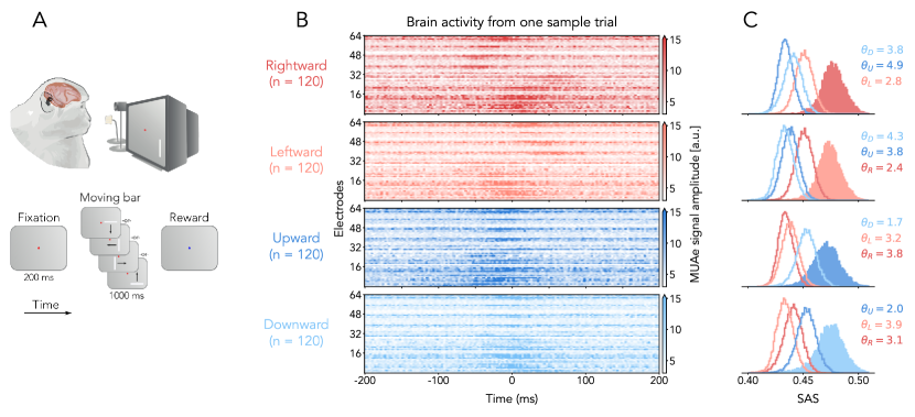
Figure 6: Comparing non-square matrices of brain activity with SAS. A Schematic diagram of the neuroscience experiment. B Single-trial brain activity at identical recording electrodes ($64$ electrodes, vertical) for each type as example (trial types distinguished by color). Larger values of matrix entries indicate higher MUAe activity (shading in color bar, arbitrary units). C Histograms of SAS between all ($n=120$) individual trials. Filled distributions (color code as in B) indicate self-similarities, non-filled ones indicate cross-similarities. Legends show effect sizes $\theta$ for the comparison between self- and cross-similarities.

We investigate brain activity originating from different experimental trials as a use case for SAS with non-square matrices of experimental data. The publicly available data set from [16] is based on extracellular recordings from the visual cortex of a macaque monkey. In the experiment, bright bars move across a screen in one of four directions (rightward (R), leftward (L), upward (U) or downward (D)), evoking a strong neural response (Figure 6A). The data consists of the multi-unit activity envelope (see Section 2) yielding one $64\times 400$ matrix per trial; sample matrices are shown in Figure 6B.

Neurons in the primary visual cortex (V1) respond according to their feature selectivity, primarily stimulus location [26] and orientation [27], but also movement direction [28]. Beyond these well-known response properties of single neurons, the population activity—represented as a two-dimensional spatio-temporal matrix—may reveal additional information about brain dynamics. By applying SAS, we investigate shared variability across both time and neurons.

In the data set at hand, SAS reveals that neural activity of all trial types exhibits higher self- than cross-similarity with effect sizes $\theta>1$ (Figure 6C). Trials with stimulus movement along the same axis (L-R or U-D) are more similar to each other than to ones with orthogonal stimulus movement. This is a desirable outcome of SAS: in L-R (resp. U-D) trials, neurons that share an orientation tuning aligned with the stimulus are expected to have a higher probability of a strong response. The consideration implies that the shared orientation of the bar stimulus in L and R (resp. U and D) trials leads to more similar responses in these trial pairs.

In this use case, SAS outperforms common measures of matrix similarity. Both cosine similarity and the Frobenius norm can distinguish trial types—albeit with lower $|\theta|$ than SAS—but fail to identify the shared variability along the same axis (L-R or U-D) (Figure S3). Therefore, the use case highlights the ability of SAS to identify the two-dimensional structure of matrices in experimental data.

4 Discussion

Here, we present singular angle similarity (SAS): a method for comparing the similarity of real matrices of identical shape based on singular value decomposition. SAS is invariant under transposition and consistent relabeling of coordinates, and reliably detects structural similarities in the compared matrices. It generalizes the angular similarity (Section S1.7) for vectors and the eigenangle score for symmetric positive definite matrices by [9]. For a particular choice of weight function and vector similarity measure, SAS and the eigenangle score are equivalent for positive-definite symmetric matrices. [9] introduce an extension of the eigenangle score for asymmetric adjacency matrices of certain network types by choosing a specific analytical mapping of the complex-valued eigenvalues and vectors: shift the real part of the eigenvalues by the spectral radius of the matrix, and calculate the Euclidean angle between the complex eigenvectors [29]. However, this choice is not unique—other mappings are also possible. In addition, the resulting similarity measure is not invariant under joint transposition of the compared matrices. In SAS, the singular vectors are real-valued, the singular values are non-negative, and the measure is transposition invariant. Thereby, it circumvents these limitations and admits a more natural generalization to non-symmetric and non-square matrices. We here choose angular similarity as the vector similarity measure, and a specific weight function for the resulting angles (Equation 8). Other choices are possible, such as cosine similarity for the former, making SAS easily adaptable.

Since SAS is sensitive to matrix size (Section 3.3) it can only be interpreted in relative terms. A quantitative reference can be obtained by choosing a use-case-specific null model (e.g. Erdős-Rényi for network models) for which the corresponding distribution of SAS can be determined numerically. Similarity as indicated by SAS can then be interpreted in terms of this baseline. Since realizations of single matrices exhibit fluctuations, evaluating SAS from a single observation may be misleading. Instead, one should consider the SAS distribution of an ensemble of realizations when possible. Such a distribution can then be interpreted with respect to the reference distribution obtained with the null model by means of an effect size (Equation 11) or a statistical two-sample test of choice.

While SAS generally highlights structural features in matrices stemming from their correlations along rows and columns, it also suffers from shortcomings in certain situations. In the presence of sufficiently strong noise, the order of singular values may change even if two matrices encode the same underlying information. This leads to a different pairing of singular vectors when computing SAS, resulting in a low score even though the matrices result from a common construction process. An alternative method for pairing singular vectors is discussed in Section S1.1. Furthermore, if two matrices have identical pairs of left and right singular vectors that are ordered identically (as defined by their singular values) but the singular values themselves exhibit a different spectrum, SAS indicates perfect similarity. While desirable in some situations, this property may lead to unexpected results in some contexts.

Beyond network connectivity or brain activity matrices, potential applications include the analysis of matrices obtained with asymmetric measures for the flow of information, like Granger Causality [30], or Transfer Entropy [31]. Additionally, SAS can help assess similarity in more classical settings, e.g., when studying cross-covariances.

In conclusion, SAS can be used to analyze the structural similarity of any real-valued data that can be represented in matrix form. Such data can come from any field of research. Coupled with domain knowledge, SAS may reveal hidden structures in the data, supporting existing methodologies and enabling new insights.

Code and data availability

Code to calculate singular angle similarity (SAS) is openly available on GitHub (https://github.com/INM-6/SAS) and Zenodo (https://doi.org/10.5281/zenodo.10680478), and in the validation test library NetworkUnit [32]. The data and code to reproduce the results from this paper can be found on Zenodo (https://doi.org/10.5281/zenodo.10680810).

Acknowledgments

This work has been supported by NeuroSys as part of the initiative “Clusters4Future” by the Federal Ministry of Education and Research BMBF (03ZU1106CB); the DFG Priority Program (SPP 2041 ”Computational Connectomics”); the EU’s Horizon 2020 Framework Grant Agreement No. 945539 (Human Brain Project SGA3); the Ministry of Culture and Science of the State of North Rhine-Westphalia, Germany (NRW-network ”iBehave”, grant number: NW21-049); the Joint Lab ”Supercomputing and Modeling for the Human Brain”.

Author contributions

Conceptualization: JA, AK, RG; Methodology: AK, JA, RG; Software: JA, RG, AK, AMG; Formal analysis: JA, AK, RG, AMG; Writing - original draft: JA, AK, RG, AMG; Writing - review & editing: all; Visualization: JA, AK, AMG, RG; Supervision: MDe, SvA, MDi; Funding acquisition: SG, SvA, MDi

S1 Supplementary materials

S1.1 Singular angle similarity based on optimal subspace alignment

As an alternative to pairing singular vectors based on the order given by the singular values, they may instead be paired such that they are optimally aligned, i.e., such that the angle between them is minimized. We define an analogous measure called SAS-VEC that uses this pairing strategy in the following. First, we introduce the generalized left and right singular angles of the first kind as

$$\alpha^{jk}(U) =\sphericalangle(u_{a}^{j},u_{b}^{k})=\arccos\left(\langle u_{a}^{j},u_{b}^{k}\rangle\right),$$

$$\quad\alpha^{jk}(V) =\sphericalangle(v_{a}^{j},v_{b}^{k})=\arccos\left(\langle v_{a}^{j},v_{b}^{k}\rangle\right).$$ (13)

and mutatis mutandis the generalized left and right singular angles of the second kind, $\alpha^{jk}(U^{-}),\alpha^{jk}(V^{-})$. With this, the generalized singular angles are

$$\alpha^{jk} =\min\left\{\frac{\alpha^{jk}(U)+\alpha^{jk}(V)}{2},\frac{\alpha^{jk}(U^{-})+\alpha^{jk}(V^{-})}{2}\right\}.$$

The sorting scheme first selects the smallest angle $\alpha^{j_{1}k_{1}}$. This angle corresponds to the pairs of left and right singular vectors $(u^{j_{1}}_{a},v^{j_{1}}_{a})$ and $(u^{k_{1}}_{b},v^{k_{1}}_{b})$ that are most jointly aligned. Next, the algorithm calculates the corresponding angular similarity $\Delta^{j_{1}k_{1}}$ weighted by $\bar{w}^{j_{1}k_{1}}=\bar{w}(\sigma_{a}^{j_{1}},\sigma_{b}^{k_{1}})$. Here, we want to capture the overlap of the aligned pairs of left and right singular vectors scaled by the singular values. Using the arithmetic mean as a weight function for the singular values is thus not suitable: if one singular value is large while the other is close to zero, the mean stays on the order of the larger value. This is not desirable since the total overlap should approach zero. Instead, we choose as a weight function

$$\bar{w}(\sigma_{a},\sigma_{b})=\sqrt{\sigma_{a}\sigma_{b}}~{}.$$ (14)

Finally the algorithm removes the column and the row of the angle matrix $\alpha^{jk}$ corresponding to the pair of first left and right singular vectors to determine $\alpha^{j_{2}k_{2}}$ of the next iteration step. If multiple pairings of vectors produce the same minimal angle, the algorithm chooses one of them at random for this iteration. This procedure continues until the angle matrix is of dimension zero. After completion, SAS-VEC results as

$$\frac{\sum_{m}\bar{w}^{j_{m}k_{m}}\Delta^{j_{m}k_{m}}}{\sum_{m}\bar{w}^{j_{m}k_{m}}}.$$ (15)

In contrast to SAS, SAS-VEC does not prioritize the vectors with the largest singular values. Instead, the measure matches those left and right singular vectors of the matrices that are most similar. Thereby, SAS-VEC assesses the alignment of the high-dimensional orthonormal bases of the data as calculated by SVD. While this avoids the issue of pairing vectors when singular values are close, SAS-VEC may overestimate similarity for noisy data, especially when the matrix dimensionality is low. For this reason, the authors suggest additional care when applying SAS-VEC.

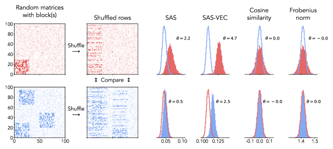
Figure S1: Example random matrices of dimension $N=100$ containing multiple blocks with correlated noise of size $30\times 30$. Between samples, new matrices are generated and the rows are shuffled randomly. The precise definition of the matrices is available in the published code (https://doi.org/10.5281/zenodo.10680810).

See Figure S1 for a comparison between SAS, SAS-VEC, cosine similarity, and the Frobenius norm on an example for which SAS-VEC yields a higher effect size than SAS.

S1.2 Invariance properties of SAS

Let $M_{a},M_{b}\in\mathbb{R}^{m\times n}$ with SVDs

$$M_{i}=U_{i}\Sigma_{i}V_{i}^{T}$$ (16)

for $i\in\{a,b\}$. Noting that the transposition of an orthogonal transformation is again orthogonal, the SVDs of $M_{i}^{T}$ are

$$M_{i}^{T}=V_{i}\Sigma_{i}^{T}U_{i}^{T}~{}.$$ (17)

Thus, by its definition, the SAS between $M_{a}$ and $M_{b}$ is invariant under transposition of both matrices. If working with the eigendecomposition instead of the SVD, one obtains, in the general case,

$$M_{i}=P_{i}\Lambda_{i}P_{i}^{-1}$$ (18)

where $\Lambda_{i}$ is a diagonal matrix containing the eigenvalues, and the columns of $P_{i}$ are the eigenvectors. Here, the eigenvectors are not guaranteed to be orthogonal. Thus,

$$({P_{i}^{-1}})^{T}\neq P_{i}$$ (19)

in general. Consequently, any measure comparing the eigenvectors is not invariant under transposition of the compared matrices. Specifically, this includes the eigenangle score [9].

Additionally, SAS is invariant under actions of identical orthogonal matrices from the left or right onto $M_{i}$. We denote the orthogonal matrices as $O_{1}$ and $O_{2}^{T}$. The action of the matrices from the left and from the rights yields

$$\tilde{M}_{i}=O_{1}M_{i}O_{2}^{T}~{},$$ (20)

and the corresponding SVD is

$$\tilde{M}_{i}=\tilde{U}_{i}\Sigma_{i}\tilde{V}_{i}^{T}=\big{(}O_{1}U_{i}\big{)}\Sigma_{i}\big{(}O_{2}V_{i}\big{)}^{T}~{}.$$ (21)

Note that the singular values remain identical. Since the left and right singular vectors of the matrices $\tilde{M}_{i}$ are $\tilde{u}_{i}^{j}=\tilde{U}_{i}e^{j}$ and $\tilde{v}_{i}^{j}=\tilde{V}_{i}e^{j}$, we compute the left and right singular angles as

$$\alpha^{j}(\tilde{U})=\arccos\left(\langle\tilde{U}_{a}e^{j},\tilde{U}_{b}e^{j}\rangle\right)=\arccos\left(\langle O_{1}U_{a}e^{j},O_{1}U_{b}e^{j}\rangle\right)=\arccos\left(\langle U_{a}e^{j},U_{b}e^{j}\rangle\right)=\alpha^{j}(U)$$ (22)

and mutatis mutandis for $\alpha^{j}(\tilde{V})$, resp. $\alpha^{j}(\tilde{U}^{-}),\alpha^{j}(\tilde{V}^{-})$. We here used the orthogonality of the matrices $O_{i}$. Thus, the singular angles, the singular values, and consequently the similarity score, are invariant under the action of orthogonal matrices from the left and the right.

S1.3 Change of SAS under scaling

Consider a matrix $M$ with SVD

$$M=U\Sigma V^{T}$$ (23)

and scalars $c_{1}>0$ as well as $c_{2}<0$. In the following, our aim is to determine the SAS between $M$ and $c_{i}M$ for $j=1,2$.

Positive scaling

We note that the SVD of $c_{1}M$ is

$$c_{1}M=U(c_{1}\Sigma)V^{T}~{}.$$ (24)

Hence, only the singular values are scaled while the left and right singular vectors remain constant. This implies $\alpha^{j}=0~{}\forall j$, and thus an angular similarity of $\Delta^{j}=1~{}\forall j$. Therefore, SAS between $M$ and $c_{1}M$ equals $1$.

Negative scaling

We write $c_{2}=-1\cdot|c_{2}|$ and determine the SVD of $c_{2}M$ as

$$c_{2}M=(-1\cdot U)|c_{2}|\Sigma V^{T}=U|c_{2}|\Sigma(-1\cdot V^{T})~{}.$$ (25)

In the following, we focus on the first of the two representations. The second one can be treated analogously. We first calculate

$$\alpha^{j}(U)=\arccos\left(\langle u^{j},-u^{j}\rangle\right)=\arccos(-1)=\pi,\quad\alpha^{j}(V)=0~{}.$$ (26)

Thus, we obtain $\bar{\alpha}^{j}=\pi/2$ and consequently $\alpha^{j}=\pi/2~{}\forall j$. Therefore, the angular similarity $\Delta^{j}=1-\alpha^{j}/\frac{\pi}{2}=0$, and the SAS between $M$ and $c_{2}M$ equals $0$.

S1.4 Change of SAS under small perturbations

Consider a matrix $M$ with SVD

$$M=U\Sigma V^{T}~{}.$$ (27)

For simplicity, we assume that $M\in\mathbb{R}^{n\times n}$ is a random matrix with non-degenerate singular values. First, we relate the singular values as well as the left and right singular vectors to the eigenvalues and eigenvectors of certain symmetric matrices. We calculate

$$MM^{T}=U\Sigma^{2}U^{T},\quad M^{T}M=V\Sigma^{2}V^{T}$$ (28)

and observe that $MM^{T}$ and $M^{T}M$ are symmetric, the squared singular values are the eigenvalues of the matrices, and since $U$ and $V$ are orthogonal matrices, the left and right singular vectors are the eigenvectors. We perturb $M$ by a random $\sqrt{\epsilon}W$, thus considering $M+\sqrt{\epsilon}W$. This induces a perturbation up to first order (in $\sqrt{\epsilon}$) of $\sqrt{\epsilon}\big{(}MW^{T}+WM^{T}\big{)}$ in $MM^{T}$ and $\sqrt{\epsilon}\big{(}M^{T}W+W^{T}M\big{)}$ in $M^{T}M$. Following Rayleigh-Schrödinger perturbation theory [24] , the perturbed left singular vectors $\tilde{u}^{j}$ read

$$\tilde{u}^{j}=u^{j}+\sqrt{\epsilon}\sum_{k\neq j}\frac{\langle u^{k},\big{(}MW^{T}+WM^{T}\big{)}u^{j}\rangle}{{\sigma^{j}}^{2}-{\sigma^{k}}^{2}}u^{k}+\epsilon\cdot\textnormal{ terms orthogonal to }u^{j}~{}.$$ (29)

while the perturbed eigenvalues are

$$\tilde{\sigma}^{{j}^{2}}=\sigma^{{j}^{2}}+\sqrt{\epsilon}\langle u^{j},\big{(}MW^{T}+WM^{T}\big{)}u^{j}\rangle+\epsilon\sum_{k\neq j}\frac{\langle u^{k},\big{(}MW^{T}+WM^{T}\big{)}u^{j}\rangle^{2}}{{\sigma^{j}}^{2}-{\sigma^{k}}^{2}}~{}.$$ (30)

To investigate how the eigenvalues change under perturbation, we calculate:

$$\langle u^{j},\big{(}MW^{T}+WM^{T}\big{)}u^{j}\rangle$$

$$= \langle u^{j},MW^{T}u^{j}\rangle+\langle u^{j},WM^{T}u^{j}\rangle$$

$$= \langle WM^{T}u^{j},u^{j}\rangle+\langle u^{j},WM^{T}u^{j}\rangle$$

$$= 2\langle WM^{T}u^{j},u^{j}\rangle$$

$$= 2\sigma^{j}\langle Wv^{j},u^{j}\rangle~{}.$$ (31)

Similarly,

$$\langle u^{k},\big{(}MW^{T}+WM^{T}\big{)}u^{j}\rangle=\sigma^{k}\langle Wv^{k},u^{j}\rangle+\sigma^{j}\langle u^{k},Wv^{j}\rangle~{}.$$ (32)

Writing the perturbation matrix $W$ as an expansion of the left and right singular vectors, we get

$$W=\sum_{j,k}\bar{w}_{jk}u^{j}(v^{k})^{T}$$ (33)

where $\bar{w}_{ij}\in\mathbb{R}$ are the corresponding coefficients. Thus

$$\tilde{\sigma}^{{j}^{2}}=\sigma^{{j}^{2}}+\sqrt{\epsilon}2\sigma^{j}\bar{w}_{jj}+\epsilon\sum_{k\neq j}\frac{\left(\sigma^{k}\bar{w}_{jk}+\sigma^{j}\bar{w}_{kj}\right)^{2}}{{\sigma^{j}}^{2}-{\sigma^{k}}^{2}}~{}.$$ (34)

Consequently, it is easy to construct perturbations that leave certain singular values unchanged. For a random perturbation, however, this is unlikely: even when the perturbation changes a single entry of $M$, since the left and right singular vectors generally have no resemblance to the standard normal basis of $\mathbb{R}^{n}$, most of the $\bar{w}_{ij}$ differ from zero. Neglecting the special case in which the first and second order exactly cancel, we can assume that all eigenvalues change under perturbation.

Writing

$$c_{kj}=\frac{\langle u^{k},\big{(}MW^{T}+WM^{T}\big{)}u^{j}\rangle}{{\sigma^{j}}^{2}-{\sigma^{k}}^{2}}~{},$$ (35)

normalizing the eigenvectors yields

$$\tilde{u}^{j}=\bigg{(}1-\frac{\epsilon}{2}\sum_{k\neq j}c_{kj}^{2}\bigg{)}u^{j}+\sqrt{\epsilon}\cdot\textnormal{ terms orthogonal to }u^{j}$$ (36)

and mutatis mutandis for the perturbed right singular vectors $\tilde{v}^{j}$. This implies for the angles between the left singular vectors of the unperturbed and perturbed matrix

$$\alpha^{j}(U) =\arccos\left(\langle u^{j},\tilde{u}^{j}\rangle\right)$$

$$=\arccos\left(\langle u^{j},\bigg{(}1-\frac{\epsilon}{2}\sum_{k\neq j}c_{kj}^{2}\bigg{)}u^{j}+\sqrt{\epsilon}\cdot\textnormal{ terms orthogonal to }u^{j}\rangle\right)$$

$$=\arccos\bigg{(}1-\frac{\epsilon}{2}\sum_{k\neq j}c_{kj}^{2}\bigg{)}$$ (37)

where we used the orthonormality of the $u^{i}$.

By a similar argument as for the eigenvalues, we can also assume that for a generic perturbation, the eigenvectors change. Thus, $\sum_{k\neq j}c_{kj}^{2}>0$ since $\langle u^{j},\tilde{u}^{j}\rangle<1$, and we denote by $C(M,W,U)$ the smallest of those terms. Hence, we obtain

$$\alpha^{j}(U)\leq\arccos(1-\epsilon C(M,W,U))$$ (38)

where the constant also absorbs the factor $\frac{1}{2}$. Since the same relations hold for the right singular vectors, we have $\alpha^{j}\leq\arccos(1-\epsilon^{2}C(M,W))$ where $C(M,W)=\min\{C(M,W,U),C(M,W,V)\}$. And as this holds true for all angles $\alpha^{j}$, it implies that SAS between the matrices $M$ and $M+\sqrt{\epsilon}W$ is $1-\arccos(1-\epsilon C(M,W))/\frac{\pi}{2}$ up to first order in $\epsilon$.

S1.5 The Perron-Frobenius Theorem and the Perron vector

The Perron-Frobenius theorem [25] for non-negative square matrices asserts that if a matrix $N$ has only non-negative entries, then

• there is a real eigenvalue $\lambda_{\mathrm{P}}\geq 0$ of $N$ such that, for all other eigenvalues $\lambda$ of $N$, $|\lambda|\leq\lambda_{\mathrm{P}}$, and

• the eigenvector corresponding to the eigenvalue $\lambda_{\mathrm{P}}$ has only non-negative entries. This eigenvector is called the Perron vector.

For the random graphs in this work, SAS considers $N=M_{i}M_{i}^{T}$ and $N=M_{i}^{T}M_{i}$ where $M_{i}$ is an adjacency matrix with non-negative entries. In both cases, $N$ is a symmetric positive-definite matrix. Both $N$ share all non-zero eigenvalues (the squares of the singular values of $M_{i}$), and the eigenvectors of $N$ are the right and left singular vectors (up to a potential multiplication with $-1$.) Since by assumption non-trivial singular values are unique, and under the assumption that at least one non-trivial singular value exists, the above inequalities become strict, and the eigenvector to $\lambda_{\mathrm{P}}$ becomes unique.

S1.6 Non-square matrices from subsampled networks

We define subsampled graphs as graphs where the connectivity is only known for a random subset of source nodes. Thus, the adjacency matrices are non-square. We keep the number of possible connections in the network the same by instantiating a full graph of size $N_{>}=\frac{1}{f}N_{N}$ where $f<1$, and then subsample $N_{<}=fN_{N}$ source nodes. For all networks we here choose $f=2/3$ and for the comparison between subsampled graphs in this work, the list of source nodes for which information is available is shared across network instance and models. We use SAS to test how similar the structures of subsampled networks are.

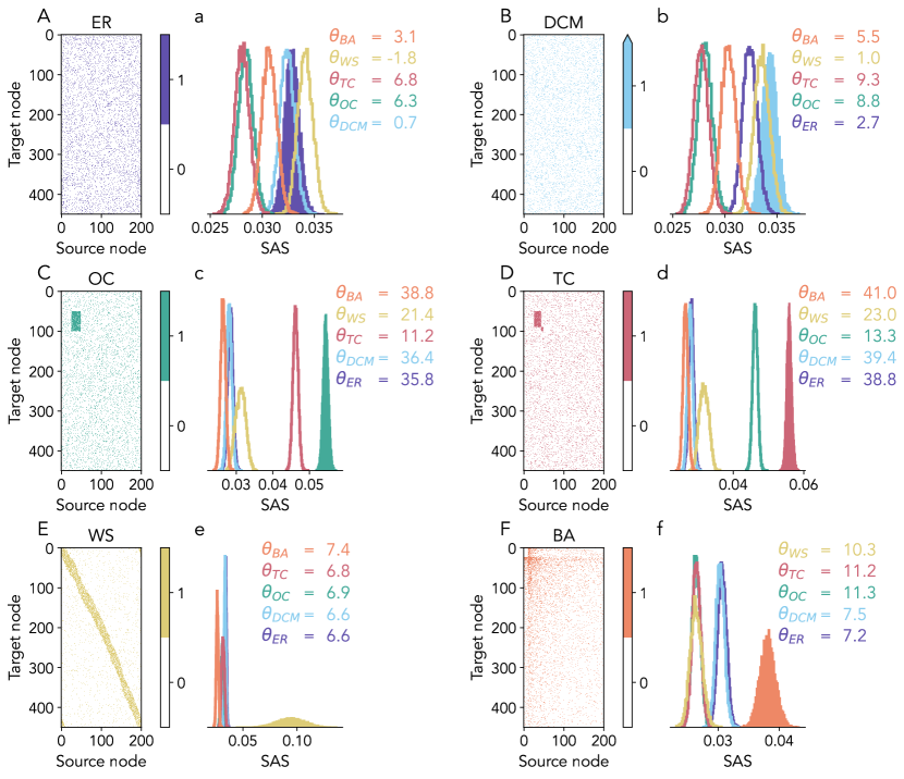
Figure S2: Self- and cross-similarity of subsampled network models. A–F Single instances of the different network models. Colored matrix elements indicate a connection between nodes. a–f Histograms of SAS between instances of the network models ($n=100$, all pairs compared). Filled distributions indicate self-similarities, non-filled ones indicate cross-similarities. Effect sizes $\theta$ between self- and cross-similarities also shown.

Instances of these subsampled graphs, their respective self- and cross-similarities, and the corresponding effect sizes are shown in Figure S2. In subsampled graphs, some of the original structure is inevitably invisible, and we therefore expect SAS to find less distinguishable structure. This is especially apparent for the directed configuration model (DCM) network, which does not have enough structure to be reliably distinguished from the other network models. All other subsampled network graphs retain enough structure such that SAS can distinguish between them.

S1.7 SAS for $1\times n$ matrices

Let $v_{i}\in\mathbb{R}^{1\times n}$ where $i\in\{a,b\}$. In this case, the SVD reads

$$v_{i}=1\cdot\mathrm{diag}(\lVert v_{i}\rVert,0,...,0)\cdot\begin{bmatrix}&\frac{v_{i}}{\lVert v_{i}\rVert}_{2}&\big{|}&\ast&\big{|}&\dots&\big{|}&\ast&\\ \end{bmatrix}~{}.$$ (39)

Thus, there is only one non-zero singular value, resulting in the weighted sum used in the definitions of SAS to consist of one summand, with weight one. Thus, SAS is the angular similarity between $v_{a}$ and $v_{b}$ in this case.

S1.8 Comparison of SAS with common measures on brain data

We here compare how similarity is assessed by SAS, cosine similarity, and the Frobenius norm between the different trial types of brain activity data (Section 2.4). Figure S3 shows that only SAS identifies that the recorded activity is more similar between trials where the stimulus has the same orientation (U-D and L-R).

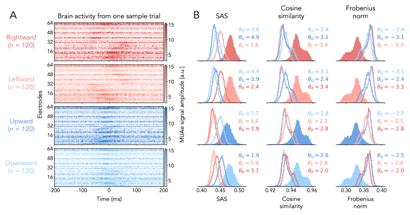
Figure S3: Comparing non-square matrices of brain activity with SAS, cosine similarity, and the Frobenius norm. A Brain activity of all recorded electrodes for one example trial of each type (different trials as shown in Figure 6). B Histograms of SAS, cosine similarity and the Frobenius norm between all individual trials. Filled distributions indicate self-similarities, non-filled ones indicate cross-similarities. Effect sizes $\theta$ for the comparison between self- and cross-similarities also shown.

References

- [1] Mark EJ Newman “The structure and function of complex networks” In SIAM Review 45.2, 2003, pp. 167–256 DOI: 10.1137/S003614450342480
- [2] Brittny Calsbeek and Charles J Goodnight “Empirical comparison of G matrix test statistics: finding biologically relevant change” In Evolution 63.10 Blackwell Publishing Inc Malden, USA, 2009, pp. 2627–2635
- [3] Ricard V. Sol and M. Montoya “Complexity and Fragility in Ecological Networks” In Proceedings of the Royal Society of London. Series B: Biological Sciences 268.1480 The Royal Society, 2001, pp. 2039–2045 DOI: 10.1098/rspb.2001.1767
- [4] Carlo Piccardi, Lisa Calatroni and Fabio Bertoni “Clustering Financial Time Series by Network Community Analysis” In International Journal of Modern Physics C 22.01 World Scientific Publishing Co., 2011, pp. 35–50 DOI: 10.1142/S012918311101604X
- [5] Peter H Schönemann “A generalized solution of the orthogonal procrustes problem” In Psychometrika 31.1 Springer, 1966, pp. 1–10
- [6] Paul Robert and Yves Escoufier “A unifying tool for linear multivariate statistical methods: the RV-coefficient” In Journal of the Royal Statistical Society Series C: Applied Statistics 25.3 Oxford University Press, 1976, pp. 257–265
- [7] Harold Hotelling “Relations Between Two Sets Of Variates” In Biometrika 28.3-4, 1936, pp. 321–377 DOI: 10.1093/biomet/28.3-4.321
- [8] Gene H Golub and Hongyuan Zha “The canonical correlations of matrix pairs and their numerical computation” In Linear Algebra for Signal Processing 69, The IMA Volumes in Mathematics and its Applications Springer, 1995 DOI: https://doi.org/10.1007/978-1-4612-4228-4˙3
- [9] Robin Gutzen, Sonja Grün and Michael Denker “Evaluating the statistical similarity of neural network activity and connectivity via eigenvector angles” In BioSystems 223 Elsevier, 2023, pp. 104813 DOI: https://doi.org/10.1016/j.biosystems.2022.104813
- [10] Lloyd N Trefethen and David Bau “Numerical linear algebra” Siam, 2022
- [11] P. Erdős and A. Rényi “On random graphs” In Publicationes Mathematicae 6, 1959, pp. 290–297
- [12] Juyong Park and Mark EJ Newman “Statistical mechanics of networks” In Physical Review E 70.6 APS, 2004, pp. 066117
- [13] Colin Cooper and Alan Frieze “The Size of the Largest Strongly Connected Component of a Random Digraph with a Given Degree Sequence” In Combinatorics, Probability and Computing 13.3 Cambridge University Press, 2004, pp. 319–337 DOI: 10.1017/S096354830400611X
- [14] D. J. Watts and S. H. Strogatz “Collective dynamics of small-world networks” In Nature 393, 1998, pp. 440–442 DOI: 10.1038/30918
- [15] Réka Albert and Albert-László Barabási “Statistical mechanics of complex networks” In Reviews of Modern Physics 74, 2002, pp. 47–97
- [16] Xing Chen et al. “1024-Channel Electrophysiological Recordings in Macaque V1 and V4 during Resting State” In Scientific Data 9.1, 2022, pp. 77 DOI: 10.1038/s41597-022-01180-1
- [17] Hans Supèr and Pieter R. Roelfsema “Chronic multiunit recordings in behaving animals: Advantages and limitations” In Progress in Brain Research 147.SPEC. ISS. Elsevier, 2005, pp. 263–282 DOI: 10.1016/S0079-6123(04)47020-4
- [18] Aitor Morales-Gregorio et al. “Neural manifolds in V1 change with top-down signals from V4 targeting the foveal region” In BioRxiv Cold Spring Harbor Laboratory, 2023, pp. 2023–06 DOI: https://doi.org/10.1101/2023.06.14.544966
- [19] Vladimir Alexandrovich Marchenko and Leonid Andreevich Pastur “Distribution of eigenvalues for some sets of random matrices” In Matematicheskii Sbornik 114.4 Russian Academy of Sciences, Steklov Mathematical Institute of Russian …, 1967, pp. 507–536
- [20] Jacob Cohen “Statistical Power Analysis for the The Behavioral Sciences” L. Erlbaum Associates, 1988, pp. 567
- [21] Student “The probable error of a mean” In Biometrika JSTOR, 1908, pp. 1–25
- [22] Bernard L Welch “The generalization of Student’s problem when several different population varlances are involved” In Biometrika 34.1-2 Oxford University Press, 1947, pp. 28–35 DOI: https://doi.org/10.1093/biomet/34.1-2.28
- [23] T Tony Cai, Jianqing Fan and Tiefeng Jiang “Distributions of angles in random packing on spheres” In Journal of Machine Learning Research 14, 2013, pp. 1837–1864 DOI: 10.1098/rspb.2001.1767
- [24] Lev Davidovich Landau and Evgenii Mikhailovich Lifshitz “Quantum mechanics: non-relativistic theory” Elsevier, 2013
- [25] Peter Deuflhard and Andreas Hohmann “Numerische Mathematik 1: Eine algorithmisch orientierte Einführung” Walter de Gruyter, 2008 DOI: 10.1515/9783110203554
- [26] Roger BH Tootell, Martin S Silverman, Eugene Switkes and Russell L De Valois “Deoxyglucose analysis of retinotopic organization in primate striate cortex” In Science 218.4575 American Association for the Advancement of Science, 1982, pp. 902–904 DOI: 10.1126/science.713498
- [27] D. H. Hubel and T. N. Wiesel “Receptive fields of single neurones in the cat’s striate cortex” In Journal of Physiology 148, 1959, pp. 574–591
- [28] Russell L De Valois, Duane G Albrecht and Lisa G Thorell “Spatial frequency selectivity of cells in macaque visual cortex” In Vision Research 22.5 Elsevier, 1982, pp. 545–559
- [29] Klaus Scharnhorst “Angles in complex vector spaces” In Acta Applicandae Mathematicae 69 Springer, 2001, pp. 95–103 DOI: 10.1023/A:1012692601098
- [30] Clive WJ Granger “Investigating causal relations by econometric models and cross-spectral methods” In Econometrica: journal of the Econometric Society JSTOR, 1969, pp. 424–438 DOI: https://doi.org/10.2307/1912791
- [31] Thomas Schreiber “Measuring information transfer” In Physical Review Letters 85.2 APS, 2000, pp. 461
- [32] Robin Gutzen et al. “Reproducible Neural Network Simulations: Statistical Methods for Model Validation on the Level of Network Activity Data” In Frontiers in Neuroinformatics 12, 2018, pp. 90 DOI: 10.3389/fninf.2018.00090