Hierarchical Light Transformer Ensembles for Multimodal Trajectory Forecasting

Abstract

Accurate trajectory forecasting is crucial for the performance of various systems, such as advanced driver-assistance systems and self-driving vehicles. These forecasts allow to anticipate events leading to collisions and, therefore, to mitigate them. Deep Neural Networks have excelled in motion forecasting, but issues like overconfidence and uncertainty quantification persist. Deep Ensembles address these concerns, yet applying them to multimodal distributions remains challenging. In this paper, we propose a novel approach named Hierarchical Light Transformer Ensembles (HLT-Ens), aimed at efficiently training an ensemble of Transformer architectures using a novel hierarchical loss function. HLT-Ens leverages grouped fully connected layers, inspired by grouped convolution techniques, to capture multimodal distributions, effectively. Through extensive experimentation, we demonstrate that HLT-Ens achieves state-of-the-art performance levels, offering a promising avenue for improving trajectory forecasting techniques.

1 Introduction

Figure 1: Illustration of a hierarchical mixture (right) compared to a classical one (left) on a sample from the Argoverse 1 dataset. Ground truth is in dark blue in both figures, forecasts are colored dashed lines, and grey dashed lines are the centerlines of road lanes. On the right figure, we display the meta-modes (3, solid lines ending with a cross) inferred from the predictions, and their associated predictions (3, of the same color). The hierarchical structure notably enables efficient prediction compression by taking only the meta-modes.

Trajectory forecasting is a cornerstone of Advanced Driver-Assistance Systems (ADAS) and Autonomous Vehicles (AV), enabling them to anticipate effectively future risks and make informed decisions [9, 4]. However, accurately predicting trajectories is challenging due to the multimodal nature of the problem, where drivers can exhibit diverse behaviors in various situations (e.g., at an intersection). Many existing methods, deployed in real-world systems, achieve satisfactory performance primarily for short-term prediction horizons, typically employing kinematics models [26]. Yet, these models struggle to incorporate contextual information and adapt to sudden variations in traffic agent motion.

Indeed, achieving a longer prediction time horizon is challenging as the model has to account for complex interactions between varying numbers of traffic agents. As the uncertainty increases when forecasting further in time, predicting a single development becomes less relevant [23, 10, 15]. In this context, providing multiple outcomes (i.e., a set of forecasts) is more attractive but adds complexity to the task [15, 13, 40]. A prevalent approach involves the utilization of Mixture Density Networks (MDNs) [5] to capture the diverse modes (i.e., local maxima) of trajectory distributions efficiently [13, 33, 32, 49]. However, such methods face challenges in determining the appropriate number of modes, which is often ill-defined, and in ensuring that all the identified modes are not redundant. For instance, when approaching an intersection (see Fig. 1), there could be two distinct modes corresponding to turning right or proceeding straight. But, additional sub-modes may arise based on driver experiences or contextual factors. Furthermore, their industrial applications to safety-critical systems remain limited as they exhibit several shortcomings, such as overconfidence which is often typical in Deep Neural Networks (DNNs) [34, 14, 30]. Mitigating those issues, ensembles are attractive to enhance model accuracy [19] and strengthen resilience to uncertainty [21]. While they have been successfully applied to trajectory forecasting tasks [40, 42, 13, 49], their advantages come with increased computational overhead.

To address these challenges, we propose a novel solution based on hierarchical multi-modal density networks (Fig. 1, right) and efficient ensemble techniques. Our approach introduces a new loss function that captures the hierarchical structure of multi-modal predictions, allowing us to represent better the diverse behaviors exhibited by vehicles, particularly in complex scenarios. Additionally, building upon previous work [22], we adapt the concept of Packed-Ensembles, initially designed for Convolutional Neural Networks, to the realm of transformer-based models and develop a framework to train ensembles of Transformers efficiently without increasing computational complexity.

Our contributions extend beyond traditional ensemble learning techniques by focusing on both accuracy and uncertainty estimation in trajectory forecasting for autonomous driving systems. We demonstrate the effectiveness of our approach through extensive experimentation on trajectory forecasting datasets [8, 48], showcasing improved performance compared to existing methods. By leveraging hierarchical multi-modal networks and packed ensemble transformers, our method represents a significant advancement in trajectory forecasting, with potential applications in real-world autonomous driving scenarios.

In summary, our contributions are the following:

• We introduce a novel density representation and associated loss function tailored for optimizing MDNs, leveraging a hierarchical structure to capture the nuanced nature of modes in trajectory forecasting.

• We devise a light ensemble framework tailored explicitly for Transformer-based architectures, significantly reducing computational overhead while maintaining forecast quality.

• Our approach, Hierarchical Light Transformer Ensembles (HLT-Ens), offers versatility by seamlessly adapting to diverse architectures, enabling them to improve their performance.

2 Related Works

2.1 Multimodal Trajectory Forecasting

When producing long-term forecasting, predicting a single forecast or an unimodal distribution is not enough. The future position distribution is more likely to follow a multimodal distribution [10, 15, 23, 13, 49]. For instance, without any prior information, the distribution density of vehicle future positions should be higher on the roads and lower outside. At the entry of an intersection, it might be relevant to estimate a trajectory for each possible direction. To that end, [26, 37] propose to approximate the modes of the distribution using several unimodal models, and [38, 13, 3, 9, 49], defines latent variables conditioning the decoder to generate a set of forecasts.

Yet, the predicted modes do not provide any information about the uncertainty around them. To better approximate aleatoric uncertainty (input data-dependent errors), researchers have turned to probabilistic approaches. In particular, generative models have been widely used. Leveraging implicit models, [23, 27, 36, 47, 29] define a sampling procedure to generate trajectories as if they were coming from the actual conditional distribution. However, there is no information on the number of samples required to cover the underlying distribution, limiting the application of such models on safety-critical applications. On the other hand, [40, 7, 10, 11, 31, 18] estimate explicitly the distribution density with Mixture Density Networks (MDNs) [5]. Although they enable flexibility to approximate uncertainties, such models are difficult to train as they suffer from training instabilities and mode collapse (i.e., several component probabilities tend to zero consistently across examples), for which we propose solutions.

On another note, there has been a growing interest in leveraging attention mechanisms to model interactions between agents and the environment, resulting in more Transformer-based approaches among the most efficient models [33, 13, 32, 1, 50] on which we focus as our approach can be applied to any transformer backbone.

2.2 Multiple Choice Learning

In multimodal trajectory forecasting, we are interested in learning several acceptable hypotheses rather than a single one. Introduced by [16], Multiple Choice Learning is a general framework for this task. It offers a means to create cooperation between multiple predictor heads. Eventually, each head becomes specialized on a subset of the data. Inspired by this approach, [24] adapted it to train true and implicit ensembles of DNNs. In particular, they introduced Stochastic Multiple Choice Learning (sMCL) [25] training scheme based on the Winner-Takes-All (WTA) loss. Although the dataset has only one realization for each input, it enables diversity among the heads. With the same objective, [35] use a shared architecture instead of several independent ones and demonstrate the benefits of MCL for multi-label tasks while having significantly fewer parameters than its ensemble counterpart. Interestingly, many recent works leveraging MDNs for multimodal trajectory forecasting employ WTA loss variants, easing the mixture optimization [49, 42, 28]. Ideally, the WTA loss leads to a Voronoi tesselation of the ground truth [35], which could be interpreted as a perfect k-means clustering. However, the k-means algorithm is known to be dependent on its initialization, which could lead to convergence problems. In addition, the WTA loss suffers from stability issues during training, referred to as hypothesis collapse, i.e., some hypotheses receive little to no gradients due to unfortunate initialization and better other hypotheses. To mitigate this issue, [35] relaxe the WTA formulation to ensure all hypotheses are slightly updated unconditionally to their performance. Yet, [28] showcase it results in non-winning hypotheses being slowly pushed to the equilibrium, creating a spurious mode in the distribution. Therefore, they introduce the Evolving WTA (EWTA) strategy, updating the top-$n$ winners instead of solely the best one and decreasing $n$ iteratively during training. To better estimate multimodal distributions, we introduce a hierarchy to capture diversity on various scales and help the optimization process.

2.3 Efficient Ensembling

As previously stipulated, ensembling techniques, such as Deep Ensemble [21] (DE), have appealing properties to enhance performance through the diversity of several independent networks. Still, the ensemble number of parameters linearly increases with its size. Implicit ensembles designate a group of methods attempting to mimic DE diversity while having much fewer parameters. In this line of work, BatchEnsemble [43] induces diversity in a single backbone by efficiently applying rank 1 perturbation matrices, each corresponding to a member. The multi-input multi-output (MIMO) approach [17] exploits the over-parametrization of DNNs by implicitly defining several subnetworks within one backbone through MIMO settings. Recently, [22] have highlighted the possibility of creating ensembles of smaller networks performing comparably with DE. However, these approaches are applied to image classification tasks based on Convolutional Neural Networks (CNN). In our work, we present an efficient way to ensemble Transformer architecture.

3 Background

In this section, we present the mathematical formalism for this work and offer a brief background on training MDNs for trajectory forecasting. Appendix 0.A summarizes the main notations.

3.1 Trajectory Forecasting

Let us consider a dataset $\mathcal{D}=\{\mathbf{X}^{i}\}^{|\mathcal{D}|}_{i=1}$, where each instance $\mathbf{X}^{i}\in\mathbb{R}^{T\times A\times 2}$ represents the trajectories of $A$ traffic agents over $T$ timesteps: $\mathbf{X}^{i}=\mathbf{X}^{i}_{1:T}=(\mathbb{X}^{i}_{1},...,\mathbb{X}^{i}_{T})$. Here, $\mathbb{X}^{i}_{t}=(\mathbf{x}^{i}_{1}(t),...,\mathbf{x}^{i}_{A}(t))$ with $x^{i}_{j}(t)\in\mathbb{R}^{2}$ denotes the position in the 2-dimensional Euclidean space of agent $j\in\llbracket 1,A\rrbracket$ at time $t\in\mathbb{N}$ for the $i$th instance in $\mathcal{D}$.

Given an observation time-horizon $t_{obs}\in\llbracket 1,T-1\rrbracket$, we define $X_{i}\coloneqq\mathbf{X}^{i}_{1:t_{obs}}\in\mathbb{R}^{t_{obs}\times A\times 2}$ and $Y_{i}\coloneqq\mathbf{X}^{i}_{t_{obs}+1:T}\in\mathbb{R}^{t_{pred}\times A\times 2}$ with $t_{pred}=T-t_{obs}$ for better legibility. Additionally, we denote $\mathbb{X}\coloneqq\mathbb{R}^{t_{obs}\times A\times 2}$, $\mathbb{Y}\coloneqq\mathbb{R}^{t_{pred}\times A\times 2}$, and $P_{\mathcal{X},\mathcal{Y}}$ the probability followed by the dataset samples. The trajectory forecasting problem aims to estimate $Y_{i}$ given $X_{i}$ using a parametric model $f_{\theta}:\mathbb{X}\to\mathbb{Y}$ of parameter $\theta\in\mathbb{R}^{n}$. Particularly, we seek the optimal parameters $\theta^{\star}$ that minimize the expected error:

$$\frac{1}{|\mathcal{D}|}\sum^{|\mathcal{D}|}_{i=1}\ell(f_{\theta}(X_{i}),Y_{i})\ \ \text{with }\ell\text{ a loss function}$$ (1)

For a large cardinality of $\mathcal{D}$, the minimum of Eq. 1 represents the conditional expectation, i.e., $f_{\theta^{\star}}(X_{i})=\mathbb{E}\left[\mathcal{Y}|\mathcal{X}=X_{i}\right]$. However, while suitable for unimodal distributions, this average may perform poorly for multimodal ones, potentially overlooking low probability density areas between modes. Given the multimodal nature of vehicle motion distributions, especially in complex scenarios such as road intersections, a multiple-mode (or modal) approach is required.

3.2 Multiple Choice Learning

Within the Multiple Choice Learning framework, we aim to capture the complexity of phenomena better by replacing a single prediction with multiple ones. Consider a predictor providing $K$ estimates:

$$f_{\theta}(X_{i})=\left(f_{\theta}^{1}(X_{i}),...,f_{\theta}^{K}(X_{i})\right)$$ (2)

A commonly used loss to optimize such models is the Winner-Takes-All (WTA) loss (or oracle loss), which computes the error $\ell$ for the closest prediction among the $K\in\mathbb{N}$ alternatives. As outlined by [35], this loss is defined it by:

$$\int_{\mathbb{X}}\sum^{K}_{k=1}\int_{\mathbb{Y}_{k}(X)}\ell\left(f_{\theta}^{k}(X),Y\right)p(X,Y)dYdX$$ (3)

where we consider a Voronoi tesselation of the space $\mathbb{Y}=\cup^{K}_{k=1}\mathbb{Y}_{k}$ induced by $K$ unknown generators $g^{k}(X)$ and the loss $\ell$:

$$\mathbb{Y}_{k}(X)=\{Y\in\mathbb{Y}\ \colon\ \ell(g^{k}(X),Y)<\ell(g^{j}(X),Y)\ \forall j\neq k\}$$ (4)

As described in [35], Eq. 3 can be understood as the aggregation of the Voronoi cell losses generated by the predictions $f_{\theta}^{k}(X)$. To help understand the behavior of this loss, [35] assume $\ell$ is the $\ell_{2}-loss$ commonly used in regression problems and demonstrate Eq. 3 is minimal when the generators $g^{k}(X)$ and the predictors $f_{\theta}^{k}(X)$ are identical, and correspond to a centroidal Voronoi tesselation (cf. Theorem 1 of [35]). Hence, minimizing this loss can be seen as a clustering in the $\mathbb{Y}$ space conditioned on some $X\in\mathbb{X}$. Applied to trajectory forecasting, it produces diverse suitable forecasts for the same observation.

3.3 Mixture Density Networks

While having a set of forecasts helps in better trajectory estimation, we can further enhance our prediction by estimating uncertainties around each hypothesis using Mixture Density Networks (MDNs) [5]. Drawing inspiration from Gaussian Mixture distributions, traditional MDNs enable uncertainty quantification by representing forecasts as a mixture of $K\in\mathbb{N}$ Gaussian distributions (components) whose parameters are predicted by DNNs. However, for trajectory forecasting, Laplace Mixture distributions are often preferred [49, 33, 50]. Thus, given an input $X\in\mathbb{R}^{t_{obs}\times A\times 2}$, an MDN forecasting model estimates the parameters of:

$$P(\mathcal{Y}|\mathcal{X}=X)=\sum_{k=1}^{K}\pi_{\theta_{k}}(X)\mbox{Laplace}(\boldsymbol{\mu}_{\theta_{k}}(X),\mathbf{b}_{\theta_{k}}(X))$$ (5)

Here, $\boldsymbol{\mu}_{\theta_{k}}(X)\in\mathbb{R}^{t_{pred}\times A\times 2}$ represents the mean of one mode of agents’ positions at each time step, $\mathbf{b}_{\theta_{k}}(X)$ denotes the associated scale parameter, and $\boldsymbol{\pi}_{\theta}(X)$ the mixture weights $(\pi_{\theta_{1}}(X),...,\pi_{\theta_{k}}(X))\in\boldsymbol{\Delta}^{K}$ with $\boldsymbol{\Delta}^{C}=\{s\in\left[0,1\right]^{C}\mid\sum^{C}_{j=1}s_{j}=1\}$ the probability simplex.

As detailed in [28], one can train MDNs using optimization strategies coming from the Multiple Choice Learning framework, by considering $f_{\theta}^{k}(X)$ to be the tuple $(\boldsymbol{\mu}_{\theta_{k}}(X),\mathbf{b}_{\theta_{k}}(X),\pi_{\theta_{k}}(X))$ and $\ell$ to be the Negative Log Likelihood (NLL).

4 Method

4.1 Hierarchical Multimodal Distribution

Trajectory prediction involves generating multi-modal forecasts using DNNs. However, determining the appropriate number of modes (denoted as $K$) for training poses a challenge as it can vary due to multiple factors and lacks intuitive guidance. Additionally, the inherent multi-modal and uncertain nature of DNNs often leads to models with large variances, resulting in unreliable predictions. To address this challenge and improve prediction stability, we propose adapting the MDN framework to a Mixture of Mixtures, thereby introducing a novel architecture termed Hierarchical Mixture of Density Networks (HMDN).

Hence, in our proposed approach, we establish a two-level hierarchy within the multimodal distribution by introducing the concept of meta-modes (Fig. 1, right). A meta-mode is constructed from classical modes and is intended to approximate them. Practically, meta-modes represent the mode cluster centroids. The mixture formed by these meta-modes is termed the meta-mixture, we have $K^{\star}$ components within the meta-mixture:

$$P_{k^{\star}}(\mathcal{Y}|\mathcal{X}=X)=\sum_{k^{\prime}=1}^{K^{\prime}}\pi_{\theta_{k^{\star},k^{\prime}}}(X)\mbox{Laplace}(\boldsymbol{\mu}_{\theta_{k^{\star},k^{\prime}}}(X),\mathbf{b}_{\theta_{k^{\star},k^{\prime}}}(X))$$ (6)

Consequently, the hierarchical multimodal distribution is equal to :

$$P(\mathcal{Y}|\mathcal{X}=X)=\sum_{k^{\star}=1}^{K^{\star}}\pi_{\theta_{k^{\star}}}(X)P_{k^{\star}}(\mathcal{Y}|\mathcal{X}=X)$$ (7)

where $\pi_{\theta_{k^{\star}}}(X)=\sum_{k^{\prime}\in K^{\prime}}\pi_{\theta_{k^{\star},k^{\prime}}}(X)$. It is noteworthy that we assume $K^{\prime}$ remains consistent across all meta-modes, although it could vary for each meta-mode. Therefore, the total number of modes is $K=K^{\star}\times K^{\prime}$. Furthermore, we define the mean and scale of the meta-modes respectively as: $\overline{\boldsymbol{\mu}}_{\theta_{k^{\star}}}(X)=\frac{1}{K^{\prime}}\sum_{k^{\prime}}\pi_{\theta_{k^{\star},k^{\prime}}}(X)\boldsymbol{\mu}_{\theta_{k^{\star},k^{\prime}}}(X)$ and $\overline{\mathbf{b}}_{\theta_{k}^{\star}}^{2}(X)=\frac{1}{2K^{\prime}}\sum_{k^{\prime}}\left(2\mathbf{b}_{\theta_{k^{\star},k^{\prime}}}^{2}(X)+\right.$ $\left.\boldsymbol{\mu}_{\theta_{k^{\star},k^{\prime}}}^{2}(X)\right)-\overline{\boldsymbol{\mu}}_{\theta_{k^{\star}}}^{2}(X)$. Introducing these meta-modes leads to more stable predictions, as demonstrated in Tab. 2. We analyze further the loss robustness to the variation of the mode number in Appendix 0.F. The following section describes the loss we developed to train an MDN with the concept of meta-modes.

4.2 Hierarchical Multimode Loss

Many existing MDN architectures rely on explicit clustering techniques, which can introduce challenges regarding robustness to changes in mode number. In contrast, our proposed approach embraces the hierarchical structure inherent in MDNs, allowing for implicit clustering. To integrate this hierarchical structure into our prediction mixture, we introduce a novel loss function aimed at softly enforcing proximity among modes belonging to the same meta-mode, termed the Hierarchical Winner-Takes-All (HWTA) loss. The HWTA loss, denoted as $\mathcal{L}$, comprises two distinct components: the meta-mode loss ($\mathcal{L}_{\text{meta}}$) and the Meta-Winner-Takes-All (MWTA) loss.

$$\mathcal{L}=\gamma\times\mathcal{L_{\text{meta}}}+(1-\gamma)\times\mathcal{L_{\text{MWTA}}}$$ (8)

with a hyperparameter $\gamma\in\left[0,1\right]$ to control the importance of both terms. We conduct a sensitivity study on this parameter in Appendix 0.D. The meta-mode loss is the NLL of the meta-mixture, considering $N\in\mathbb{N}$ as the number of meta-modes:

$$\mathcal{L}_{\text{meta}}=\frac{1}{|D|}\sum^{|D|}_{i=1}\sum^{K^{\star}}_{k^{\star}=1}-\text{log}\left(\pi_{\theta_{k^{\star}}}(X_{i})\times\mbox{Laplace}(\overline{\boldsymbol{\mu}}_{\theta_{k^{\star}}}(X_{i}),\overline{\mathbf{b}}_{\theta_{k^{\star}}}(X_{i}))\right)$$ (9)

This term acts as a regularizer encouraging modes having the same meta-mode to be close to each other.

$\mathcal{L_{\text{MWTA}}}$ represents the Negative Log-Likelihood (NLL) of the modes belonging to the meta-mode with the lowest error. Let $k^{*}\in[1,K^{\star}]$ denote the index of the optimal meta-mode given $X_{i}$. We drop the input $X_{i}$ in the following notation for better legibility.

$$\mathcal{L}_{\text{MWTA}}=\frac{1}{|D|}\sum^{|D|}_{i=1}\frac{1}{\pi_{\theta_{k^{*}}}}\sum^{K^{\prime}}_{k^{\prime}=1}-\text{log}\left(\pi_{\theta_{k^{*},k^{\prime}}}\times\mbox{Laplace}(\boldsymbol{\mu}_{\theta_{k^{*},k^{\prime}}},\mathbf{b}_{\theta_{k^{*},k^{\prime}}})\right)$$ (10)

In addition, we add to both terms a classification loss such as the Cross-Entropy loss to optimize the mixture component weights. We provide more details on the HWTA loss in Appendix 0.C.

4.3 Hierarchical Light Transformer Ensemble

Trajectory forecasting models increasingly rely on Transformer architectures [41] due to their ability to capture spatial and temporal correlations effectively. Ensemble methods have shown promise in enhancing the performance of these DNNs. However, like in other domains, the growing size of models poses computational challenges when ensembling. To address this, we propose leveraging the over-parameterization inherent in DNNs [12] to construct ensembles of lighter Transformer-based architectures while preserving their representational capacity comparable to larger models. A crucial consideration in ensembling trajectory forecasting DNNs is the linear increase in parameters with the number of ensemble members. Packed Ensemble techniques [22] have been demonstrated to be an efficient ensembling of light Convolutional Neural Networks. Our focus is on adapting these principles for Transformer architectures, addressing the challenge of efficiently ensembling these models. In particular, we pioneered the introduction of the Grouped Multi-head Attention Layer. Using our loss HWTA, we introduce two ensemble-based variants of our techniques: HT-Ens, a straightforward ensemble of DNNs for trajectory prediction trained with HWTA, and HLT-Ens: a lightweight version of HT-Ens that we developed using the Grouped Multi-head Attention Layer.

Grouped Fully-Connected:

To encapsulate several smaller fully-connected layers into a larger one, we use Grouped Fully-Connected (GFC) layers. This concept draws inspiration from the idea that grouped convolutions [20] enable the simultaneous training of multiple branches in parallel, as demonstrated in prior works [46, 22]. The idea is to map a portion of the input to a portion of the output without any overlap.

Let us define the feature maps $\mathbf{h}^{j}\in\mathbb{R}^{D_{j}}$. Assuming we are able to split the embedding dimension $D_{j}$ into $G$ even parts, i.e., $\forall j\in\mathbb{N}$, $\mathbf{h}^{j}=\text{concat}(\mathbf{h}^{j}_{1},...,\mathbf{h}^{j}_{G})$, we create the weight tensors of a GFC layer:

$$W^{j}_{g}\in\mathbb{R}^{\frac{D_{j}}{G}\times\frac{D_{j+1}}{G}},\forall g\in\llbracket 1,G\rrbracket$$ (11)

with $G\in\mathbb{N}$ the number of groups and $j\in\mathbb{N}$ the layer’s index. The output $\mathbf{h}^{j+1}$ of the grouped fully-connected operation is:

$$\mathbf{h}^{j+1} =\text{GFC}(\mathbf{h}^{j};W^{j}_{1},...,W^{j}_{G})$$ (12)

$$=\text{concat}(\mathbf{h}^{j}_{1}W^{j}_{1},...,\mathbf{h}^{j}_{G}W^{j}_{G})$$ (13)

$$=\mathbf{h}^{j}\text{diag}(W^{j}_{1},...,W^{j}_{G})$$ (14)

$$=\mathbf{h}^{j}W^{j}$$ (15)

The transition from Eq. 13 to Eq. 15 is made by the creation of a block diagonal weight matrix $W^{j}\in\mathbb{R}^{D_{j}\times D_{j+1}}$. Fig. 2 illustrates this matrix for $G=2$. For memory efficiency, only $W_{1}$ and $W_{2}$ matrices are stored, dividing by $2$ the number of parameters required by the linear projection. Note that we omit the bias for brevity, as it is left unchanged.

Figure 2: Block diagonal weight matrix for a Grouped Fully-Connected layer with $G=2$ groups (Note: only the non-zero weights are stored in memory).

Figure 3: Grouped Multi-head Attention layer operations for $H=2$ and $G=3$. Step 1 computes the query, key, and value features for each head using grouped fully-connected layers to ensure independence between all three groups. Step 2 depicts attention mechanisms for each group in each head. Step 3 illustrates the projection of the concatenation of the heads using a grouped fully-connected layer.

Grouped Multi-head Attention:

Consider $Q\in\mathbb{R}^{n\times d_{q}}$ a query matrix, corresponding to $n\in\mathbb{N}$ query vectors of dimension $d_{q}\in\mathbb{N}$. Using $n_{v}\in\mathbb{N}$ key-value pairs with dimensions $d_{v}\in\mathbb{N}$, denoted as $K\in\mathbb{R}^{n_{v}\times d_{q}}$ and $V\in\mathbb{R}^{n_{v}\times d_{v}}$ respectively, the attention function $\text{Att}(Q,K,V)$ is defined as follows: $\text{Att}(Q,K,V)=(QK)^{T}V$.

Vaswani et al. [41] extended this operation by introducing Multi-head attention. This approach simultaneously applies $H\in\mathbb{N}$ attention functions in parallel, each operating on distinct segments of the embedding dimensions. The hyperparameter $H$ can be analogously interpreted, akin to the concept of groups previously introduced, as all heads are computed in parallel. Utilizing the shared $Q$, $K$, and $V$, the multi-head attention function is expressed as:

$$\text{MultiHead}(Q,K,V) =\text{concat}(O_{1},...,O_{H})W^{O},$$ (16)

$$\text{where }O_{h} =\text{Att}(QW^{Q}_{h},KW^{K}_{h},VW^{V}_{h})$$ (17)

$\forall h\in\llbracket 1,H\rrbracket$ and $d\in\mathbb{N}$, $W^{Q}_{h}$, $W^{K}_{h}\in\mathbb{R}^{d_{q}\times d^{H}_{q}}$ , $W^{V}_{h}\in\mathbb{R}^{d_{v}\times d_{v}^{H}}$, and $W^{O}\in\mathbb{R}^{d_{v}\times d}$ are learnable parameters. Often, in practice, $d^{H}_{q}=d_{q}/H$, $d^{H}_{v}=d_{v}/H$, and $d_{q}=d$. For better legibility, let us assume $d_{q}=d_{v}=d$ and use only $d$ as the embedding dimension.

We want to create a grouped version of the multi-head attention function, thus ensuring independence between subnetworks. Similarly to the GFC layer, we assume the embedding dimensions $d$ of $Q$, $K$, and $V$ are divisible by $G\times H$. For the following, we will only detail the operations $Q$ as they are exactly the same for $K$ and $V$. With $Q=\text{concat}(Q_{1},...,Q_{G})$, we define the $G\times H$ learnable parameters for the heads, i.e., $W^{Q}_{g,h}\in\mathbb{R}^{d_{G}\times d^{H}_{G}}$ where $g\in\llbracket 1,G\rrbracket$, $d_{G}=d/G$, and $d^{H}_{G}=d/(GH)$. We apply our previously defined GFC operation on $Q$ for each head $h$ to obtain $Q^{\prime}_{h}$:

$$Q^{\prime}_{h} =\text{GFC}(Q;W^{Q}_{1,h},...,W^{Q}_{G,h})$$ (18)

$$=\text{concat}(Q_{1}W^{Q}_{1,h},...,Q_{G}W^{Q}_{G,h})$$ (19)

Similarly we define $K^{\prime}_{h}$ and $V^{\prime}_{h}$. Using the terms in Eq. 19, we define the Grouped Multi-head Attention (GMHA) (cf. Fig. 3) operation as:

$$\text{GMHA}(Q,K,V) =\text{concat}(O^{1},...,O^{G})W^{O}$$ (20)

$$\text{where }O^{g} =\text{concat}(O^{g}_{1},...,O^{g}_{H}),$$ (21)

$$\text{and }O^{g}_{h} =\text{Att}(Q_{g}W^{Q}_{g,h},K_{g}W^{K}_{g,h},V_{g}W^{V}_{g,h})$$ (22)

Note that here, $W^{O}$ is the resulting block diagonal matrix from a GFC layer tensor weights as defined in Eq. 15. In our architecture, the number of groups corresponds to the number of subnetworks $M$ in our ensemble. As stacking grouped operations until the end ensures the independence between gradients, we will have independent subnetworks as long as other operations, such as Layer Normalization [2], can be grouped (e.g., Group Normalization [45] instead of Layer Normalization) or have independent actions on each element in the embedding dimension.

Number of parameters:

By replacing fully connected and multi-head attention layers with their grouped counterpart, we reduce the size of the overall architecture. It comes down to the parameter reduction done in the GFC layer. In a classic fully connected layer, the weight matrix encapsulates $D_{j}\times D_{j+1}$ parameters. On the other hand, GFC has $G$ weight matrices containing $D_{j}\times D_{j+1}\times G^{-2}$ parameters, meaning that divide the number of parameters by the number of groups $G$. Hence, if we were to use groups to fit subnetworks within a DNN backbone, the size of the ensemble would decrease as its number of members increases. To tackle this problem, we introduce a parameter $\alpha\in\mathbb{R}$ to compensate for the effect of using groups. It can be interpreted as a width expansion factor affecting the embedding dimension size. This enables a more flexible control of the ensemble size. The sensitivity analysis corresponding to this hyper-parameter can be found in Appendix 0.E.

5 Experiments

This section reports our experiments to validate the properties of our proposed contributions to trajectory forecasting tasks. Our evaluation focuses on assessing the accuracy of the predictions and the uncertainty estimates associated with the distribution of the resulting mixture of predictions. We provide a performance comparison of two Transformer-based backbones to showcase the benefits of both our loss and efficient ensembling architecture on trajectory forecasting tasks. Training procedures are the same for all methods sharing the same backbone, we report the hyperparameters in Appendix 0.B.

5.1 Trajectory Forecasting

Table 1: Performance comparison (averaged over five runs) on Interaction and Argoverse 1 using AutoBots and ADAPT backbones. All ensembles have $M=3$ subnetworks and are followed by a KMeans algorithm to form $6$ trajectory clusters from which we take the centroids; we highlight the best performances in bold. For our method, we consider $\alpha=1.5$ for AutoBots network and $\alpha=2$ for ADAPT network. The number of parameters is expressed in millions. M.A. corresponds to the inference cost, i.e., the number of Mega multiply-add operations for a forward pass, which is estimated with the python package torchinfo [39].

		Method	$\text{mADE}_{1}$ $\downarrow$	$\text{mADE}_{3}$ $\downarrow$	$\text{mADE}_{6}$ $\downarrow$	$\text{mFDE}_{1}$ $\downarrow$	$\text{mFDE}_{3}$ $\downarrow$	$\text{mFDE}_{6}$ $\downarrow$	b-$\text{mFDE}_{6}$ $\downarrow$	$\text{NLL}_{3}$ $\downarrow$	$\text{NLL}_{6}$ $\downarrow$	Acc $\uparrow$	#Prm $\downarrow$	M.A. $\downarrow$
Interaction	AutoBots	Single
		Legacy	0.67	0.41	0.27	1.95	1.11	0.66	1.30	-33.70	-60.18	23.12
		WTA	0.65	0.40	0.28	1.92	1.12	0.70	1.38	-33.18	-68.64	19.94
		$\varepsilon$-WTA	0.65	0.40	0.28	1.88	1.12	0.70	1.36	-44.72	-68.23	21.54
		EWTA	0.59	0.39	0.28	1.72	1.11	0.70	1.38	-34.85	-65.99	20.24
		HWTA (Ours)	0.57	0.35	0.26	1.69	0.97	0.68	1.36	-52.65	-69.50	19.42	1.2	15.22
		Ensemble
		DE	0.63	0.38	0.27	1.86	1.03	0.67	1.29	-41.23	-50.93	30.06	3.6	45.66
		HT-Ens (Ours)	0.56	0.33	0.25	1.66	0.92	0.63	1.25	-54.65	-61.97	27.05	3.6	45.66
		HLT-Ens (Ours)	0.60	0.35	0.27	1.78	0.97	0.68	1.31	-51.69	-58.03	26.92	0.9	11.62
	ADAPT	Single
		Legacy	0.71	0.43	0.30	1.97	1.15	0.73	1.37	-30.43	-55.14	23.32
		WTA	0.71	0.45	0.31	1.97	1.18	0.75	1.41	-27.00	-53.94	22.46
		$\varepsilon$-WTA	0.74	0.45	0.31	2.05	1.20	0.75	1.42	-28.61	-52.93	21.03
		EWTA	0.64	0.43	0.33	1.82	1.16	0.82	1.50	-33.54	-50.99	23.33
		HWTA (Ours)	0.63	0.40	0.30	1.78	1.08	0.73	1.35	-26.92	-53.11	23.18	1.4	1.27
		Ensemble
		DE	0.70	0.39	0.29	1.94	1.02	0.70	1.32	-41.37	-50.27	26.37	4.2	3.81
		HT-Ens (Ours)	0.63	0.36	0.28	1.79	0.95	0.69	1.32	-47.2	-55.3	27.17	4.2	3.81
		HLT-Ens (Ours)	0.56	0.37	0.29	1.62	1.00	0.72	1.31	-45.34	-54.69	32.25	2.0	0.86
Argoverse 1	AutoBots	Single
		Legacy	1.65	1.07	0.77	3.66	2.07	1.18	1.83	57.15	33.03	19.11
		WTA	1.85	1.08	0.78	4.09	2.14	1.25	1.93	52.41	27.00	17.16
		$\varepsilon$-WTA	1.76	1.08	0.80	3.87	2.16	1.30	1.98	50.45	27.58	16.75
		EWTA	2.22	1.11	0.81	4.87	2.16	1.26	1.95	51.03	32.26	16.66		17.24
		HWTA (Ours) ($K^{\star}=3$,$K=9$)	1.55	0.99	0.78	3.44	1.91	1.22	1.89	43.33	30.41	20.10	1.5	20.27
		Ensemble
		DE	1.59	0.99	0.77	3.54	1.88	1.21	1.85	44.35	35.57	27.24	4.4	51.71
		DE($K=9$)	1.62	0.98	0.81	3.59	1.85	1.35	1.95	44.09	37.82	29.79	4.5	60.80
		HT-Ens (Ours) ($K^{\star}=3$,$K=9$)	1.54	0.95	0.76	3.43	1.82	1.19	1.85	39.28	30.26	24.60	4.5	60.80
		HLT-Ens (Ours) ($K^{\star}=3$,$K=9$)	1.57	0.96	0.78	3.50	1.82	1.27	1.88	43.00	35.67	29.75	1.1	15.48
	ADAPT	Single
		Legacy	1.89	1.15	0.85	4.27	2.30	1.40	2.08	58.02	34.39	18.29
		WTA	1.84	1.13	0.83	4.13	2.29	1.38	2.07	56.65	33.14	18.57
		$\varepsilon$-WTA	1.89	1.11	0.83	4.23	2.22	1.38	2.07	55.56	33.34	18.94
		EWTA	1.80	1.15	0.84	4.00	2.33	1.40	2.09	58.74	34.40	18.49
		HWTA (Ours)	1.61	1.07	0.84	3.58	2.13	1.37	2.05	55.10	35.20	19.91	1.4	1.27
		Ensemble
		DE	1.98	1.09	0.82	4.42	2.15	1.36	2.02	46.67	37.32	23.87	4.2	3.81
		HT-Ens (Ours)	1.83	1.02	0.81	4.07	1.99	1.31	1.97	42.67	34.98	24.21	4.2	3.81
		HLT-Ens (Ours)	1.54	1.00	0.78	3.40	1.94	1.24	1.88	40.97	31.12	23.69	2.0	0.86

Datasets:

We evaluate our method’s performance in a single agent setting on Argoverse v1.1 [8] and Interaction [48]. We provide additional experiments in Appendix 0.H. Argoverse 1 Motion Forecasting is a dataset that allows us to train a model on a vast collection of $323,557$ scenarios of $5$ seconds each. Each scenario is a 2D bird-eye-view of the scene, tracking the sampled object at $10$Hz. The Agoverse v1.1 challenge is to predict $3$ seconds trajectory forecasting using $2$ seconds of the past trajectory. The Interaction dataset contains road traffic data splitter from $11$ locations recorded using drones or fixed cameras. The recordings are split into scenarios of $4$ seconds at a $10$Hz frequency. The Interaction challenge proposes to predict $3$ seconds of motion trajectory using $1$ second of prior observations.

Baselines:

To conduct our experiments on the Argoverse 1 and Interaction datasets, we leverage two light Transformer-based backbones: AutoBots [13] and ADAPT [1]. First, we compare our loss, HWTA, to the classical WTA, the relaxed WTA ($\varepsilon$-WTA), and the Evolving WTA (EWTA) losses as well as the original losses used to train the backbones we are using (we denote these as the Legacy loss). All methods set the number of modes to $6$ ($K=6$), and our approach considers $2$ meta-modes ($K^{\star}=2$ and $K^{\prime}=3$) unless otherwise indicated. Then, to demonstrate the possibility of reducing the number of parameters in an ensemble of Transformer models, we report the performance of baseline ensembles (DE), ensembling of hierarchical transformers (HT-Ens), and our hierarchical light ensembling (HLT-Ens). We post-process the outputs of methods producing more than $6$ modes using the K-Means algorithm on the final predicted positions to get $6$ trajectories.

Metrics:

We evaluate our models using standard metrics in the field [8, 6, 44, 48], including minimum Average Displacement Error ($\text{mADE}_{k}$), minimum Final Displacement Error ($\text{mFDE}_{k}$), and Brier-minimum Final Displacement Error ($\text{b-mFDE}_{k}$). Subscript $k$ denotes that these metrics are calculated over the top-$k$ most confident forecasted trajectories. We define the best trajectory as the one having the closest endpoint to the ground truth over the $k$ trajectories. $\text{mADE}_{k}$ measures the average position-wise $\ell_{2}$ distance between the ground-truth and the best predicted trajectory. $\text{mFDE}_{k}$ corresponds to the $\ell_{2}$ distance between the ground-truth endpoint and the best trajectory one. The $\text{b-mFDE}_{k}$ is slightly different as it accounts for the predicted probability $p$ of the best trajectory, i.e., $\text{b-mFDE}_{k}=(1-p)^{2}+\text{mFDE}_{k}$. In addition to that, we propose to study the $\text{NLL}_{k}$ and the mode accuracy $Acc$. We define the latter as the number of times the most confident forecast is the closest to the ground truth over the total number of samples.

Tab. 1 presents the average performance on the Argoverse 1 and the Interaction datasets over five runs. Using baseline architectures, HWTA consistently achieves attractive results compared to other optimization strategies on most metrics, especially in terms of $\text{mADE}_{1}$, $\text{mADE}_{3}$, $\text{mFDE}_{1}$, and $\text{mFDE}_{3}$. It demonstrates the ability of our loss to focus on high-probability density areas while retaining enough diversity to perform comparably with other methods. Concerning ensembling approaches, it is interesting to see that their benefits in terms of forecasting accuracy are most visible on $\text{mADE}_{k}$ and $\text{mFDE}_{k}$ with $k\in\{3,6\}$. Yet, they consistently improve the accuracy (Acc) of the models demonstrating the enhancement of mixture weights as the most confident mode is more often matched with the best one.

Concerning HLT-Ens, its application to ADAPT outperforms the baseline ensemble counterpart by a large margin on $\text{mADE}_{1}$ and $\text{mFDE}_{1}$, and achieves similar results on other metrics, using a small fraction of the parameters and number of operations required by the other ensembles. The application to AutoBots provides also good results compared to DE, with much fewer parameters, but in contrast, seems to underperform slightly compared to HT-Ens. We argue that it might be the symptom of a representation capacity too small to be subdivided into $3$ networks. In Appendix 0.E, we discuss the influence of the representation capacity, and in Appendix 0.G, we provide more insight into the differences between HLT-Ens and DE in the context of trajectory forecasting.

Tab. 2 demonstrates an improved stability induced by our loss in the optimization process. As WTA losses focus on the best prediction, the performance on the $\text{mADE}_{6}$ and $\text{mFDE}_{6}$ are consistent, i.e., low standard deviation across runs. However, we observe a higher performance variation on both $\text{mADE}_{1}$ and $\text{mFDE}_{1}$ suggesting instabilities in the optimization process. Concerning HWTA, in contrast, the standard deviation is much lower demonstrating the ability of our new loss to achieve consistent results across training runs.

Table 2: Standard deviation on metrics over five runs. This table reports the standard deviation of performance for WTA-based losses on the $\text{mADE}_{k}$ and $\text{mFDE}_{k}$ with $k=\{1,6\}$ metrics. Note the hyperparameters are the same as in Tab. 1.

		Argoverse 1				Interaction
		$\text{mADE}_{1}$	$\text{mADE}_{6}$	$\text{mFDE}_{1}$	$\text{mFDE}_{6}$	$\text{mADE}_{1}$	$\text{mADE}_{6}$	$\text{mFDE}_{1}$	$\text{mFDE}_{6}$
AutoBots	WTA	0.25	0.01	0.54	0.02	0.02	0.00	0.04	0.01
	$\varepsilon$-WTA	0.22	0.02	0.46	0.04	0.03	0.01	0.09	0.02
	EWTA	0.14	0.03	0.35	0.05	0.03	0.01	0.05	0.02
	HWTA	0.07	0.02	0.14	0.02	0.01	0.01	0.03	0.03
ADAPT	WTA	0.14	0.03	0.35	0.09	0.04	0.02	0.08	0.05
	$\varepsilon$-WTA	0.05	0.04	0.15	0.12	0.02	0.03	0.03	0.03
	EWTA	0.12	0.04	0.24	0.10	0.02	0.02	0.04	0.04
	HWTA	0.04	0.03	0.08	0.08	0.01	0.01	0.02	0.02

6 Conclusion

In conclusion, our proposed loss and ensembling framework, HLT-Ens, introduces a novel and efficient approach to multimodal trajectory forecasting, achieving state-of-the-art under identical experimental conditions. HLT-Ens leverages a hierarchical density representation and associated loss to train Mixture Density Networks and benefits from efficient ensemble training inspired by grouped convolutions.

In light of these advancements, HLT-Ens emerges as a promising approach with the capacity to enhance the performance and robustness of multimodal trajectory forecasting systems. This innovation opens avenues for improved decision-making in autonomous systems and related domains, marking a significant step forward in the evolution of trajectory prediction methodologies.

Appendix 0.A Notations

Tab. 3 summarizes the main notations used throughout this paper.

Table 3: Summary of the main notations of the paper.

Notations	Meaning
$\mathcal{D}=\{\mathbf{X}^{i}_{1:T}\}$	The set of $|\mathcal{D}|$ agents’ trajectories lasting $T$ time steps
$A$	The number of agents
$T$	The number of time steps
$K$	The number of modes, i.e., components in the mixture distribution
$K^{\star}$	The number of meta-modes, i.e., components in the meta-mixture distribution
$K^{\prime}$	The number of modes within a meta-mixture component
$a,t,k$	The indexes of the current agent, the current time step, the current mode
$X_{i}=\mathbf{X}^{i}_{1:t}$	The observed trajectories assuming $t$ steps of context
$Y_{i}=\mathbf{X}^{i}_{t+1:T}$	The target trajectories (i.e., ground-truth of the forecasts) assuming $t$ steps of context
$H$	The number of attention heads in multi-head attention layers
$M$	The number of estimators in an ensemble, i.e., ensemble size
$\theta_{k}$	The set of weights of the $k$th-component of a parametric probabilistic mixture model
$\alpha$	The width-augmentation factor of HLT-Ens.
$P_{\theta}$	The probability density function of a parametric model where $\theta$ are the parameters
$\boldsymbol{\mu}_{\theta_{k}}$	The mean of the $k$th-component of a Laplace mixture distribution parametrized by $\theta$
$\mathbf{b}_{\theta_{k}}$	The scale vector of the $k$th-component of a Laplace mixture distribution parametrized by $\theta$
$\boldsymbol{\pi}_{\theta}$	The probability vector corresponding to the mixture weights
$\overline{\boldsymbol{\mu}}_{\theta_{k^{\star}}}$	The mean of the $k$th meta-mode of a Laplace mixture distribution parametrized by $\theta$
$\overline{\mathbf{b}}_{\theta_{k^{\star}}}$	The scale vector of the $k$th meta-mode of a Laplace mixture distribution parametrized by $\theta$
$\boldsymbol{\Delta}^{C}$	The probability simplex in the $\mathbb{R}^{C}$ space

Appendix 0.B Implementation and Training Details

Table 4: Hyperparameters summary for both AutoBots and ADAPT backbones across all two datasets

		Argoverse 1		Interaction
Parameter	Description	AutoBots	ADAPT	AutoBots	ADAPT
$d$	Hidden dimension used in all model layers	128	128	128	128
Batch size	Batch size during training	128	128	128	128
Epochs	Number of epochs during training	30	36	60	36
Learning rate	Adam Optimizer initial learning rate	7.5e-4	7.5e-4	7.5e-4	7.5e-4
Decay	Multiplicative factor of learning rate decay	0.5	0.15	0.5	0.15
Milestones	Epoch indices for learning rate decay	5,10,15,20	25,32	10,20,30,40,50	25,32
Dropout	Dropout rate in multi-head attention layers	0.1	0.1	0.1	0.1
$K$	Number of modes of the baselines	6	6	6	6
$H$	Number of attention heads	16	8	16	8
$K^{\star}$	Number of meta-modes for our approaches	3	2	2	2
$K^{\prime}$	Number of modes within a meta-mode for our approaches	3	3	3	3
$\alpha$	Width factor of HLT-Ens	1.5	2.0	1.5	2.0
$\gamma$	Tradeoff of the HWTA loss	0.6	0.6	0.6	0.6

This section details both the implementation and training procedure of our models concerning the experiments. Upon acceptance and with the validation of our industrial sponsor, we expect to release the corresponding code. We implement all networks using the PyTorch framework and leverage a Nvidia RTX A6000 to train them. For both datasets, we used the same simple preprocessing:

1. We transform all agents and lanes coordinates into a scene-centric view, which is centered and oriented based on the last observed state of a focal agent, i.e., an agent having a complete track over the scene duration.

2. We keep only the $6$ closest agents to the origin.

3. We keep only the $100$ closest lanes to the origin.

Tab. 4 summarizes the hyperparameters of all our experiments. Concerning the $\varepsilon-WTA$ loss, we used $\varepsilon=0.05$ as specified in [35]. For the EWTA loss, we set up the decay over the top-$n$ modes as described in Tab. 5.

Table 5: Hyperparameter for the EWTA loss. This table reports the epoch indices where the number of modes ($n$) to update is decremented by $1$. At initialization $n=6$.

Backbones	Argoverse 1	Interaction
AutoBots	5,10,15,20,25	10,20,30,40,50
ADAPT	5,10,15,20,25	5,10,15,20,25

Appendix 0.C HWTA Loss Details

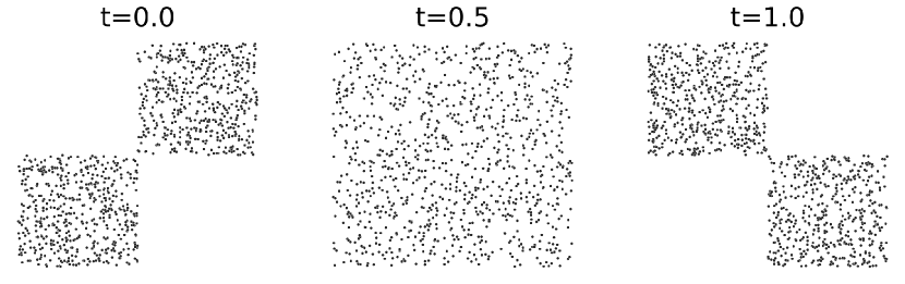
(a) Ground truth distribution

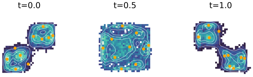
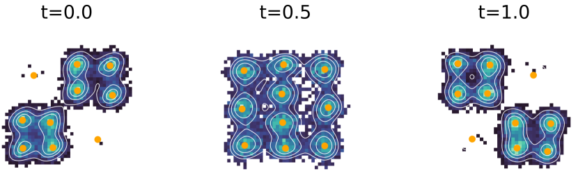
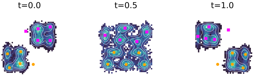
(b) Predicted distributions of small MLP models using the mixture NLL loss (top), the WTA loss with the NLL (center), and the HWTA loss with two meta-modes (in magenta and orange) (bottom)

Figure 4: Temporal 2D distributions

This section provides more explanations and insights on the HWTA loss. First, we present how classification loss terms are encompassed within the meta-mode loss and the MWTA loss. Then we illustrate our loss behavior on a 2D toy dataset (Fig. 4).

Sec. 4 defines both terms in HWTA loss as the NLL loss of the meta-mixture and the best meta-mode mixture, respectively. Yet, in practice, these terms are combined with a classification loss. Indeed, we leverage the loss formulation in [13] to define $\mathcal{L}^{\mathcal{C}}_{meta}$ and $\mathcal{L}^{\mathcal{C}}_{\text{MWTA}}$:

$$\mathcal{L}^{\mathcal{C}}_{meta} =\frac{1}{K^{\star}}\sum_{Z^{\star}}D_{\text{KL}}(Q(Z^{\star})||P_{\theta}(Z^{\star}|Y,X))$$ (23)

$$\mathcal{L}^{\mathcal{C}}_{\text{MWTA}} =\frac{1}{K^{\prime}}\sum_{Z^{\prime}}D_{\text{KL}}(Q(Z^{\prime})||P_{\theta}(Z^{\prime}|Y,X)),$$ (24)

where $Z^{\star}$ and $Z^{\prime}$ are discrete latent variables corresponding to the meta-modes and their respective modes. $D_{\text{KL}}(.||.)$ is the Kullback-Leibler divergence between the approximated posterior and the actual posterior. As in [13], we set $Q(Z^{\star})=P_{\theta_{\text{old}}}(Z^{\star}|Y,X)$ and $Q(Z^{\prime})=P_{\theta_{\text{old}}}(Z^{\prime}|Y,X)$, where $\theta_{\text{old}}$ are the parameters before the optimization step. Eq. (7) becomes:

$$\mathcal{L}=\gamma\times(\mathcal{L_{\text{meta}}}+\mathcal{L}^{\mathcal{C}}_{meta})+(1-\gamma)\times(\mathcal{L_{\text{MWTA}}}+\mathcal{L}^{\mathcal{C}}_{\text{MWTA}})$$ (25)

Inspired by [35], we utilize their custom toy dataset, which comprises a two-dimensional distribution evolving over time $t\in\left[0,1\right]$. They achieve this by dividing a zero-centered square into $4$ equal regions and transitioning from having high probability mass in the lower-left and top-right quadrants to having high probability mass in the upper-left and lower-right ones. Following their notation, the sections are defined as:

$$S_{1} =\left[-1,0\right[\times\left[-1,0\right[\subset\mathbb{R}^{2}$$ (26)

$$S_{2} =\left[-1,0\right[\times\left[0,1\right]\subset\mathbb{R}^{2}$$ (27)

$$S_{3} =\left[0,1\right]\times\left[-1,0\right[\subset\mathbb{R}^{2}$$ (28)

$$S_{4} =\left[0,1\right]\times\left[0,1\right]\subset\mathbb{R}^{2}$$ (29)

$$S_{5} =\mathbb{R}^{2}\backslash\{S_{1}\cup S_{2}\cup S_{3}\cup S_{4}\}$$ (30)

and their respective probabilities being $P(S_{1})=P(S_{4})=\frac{1-t}{2}$, $P(S_{2})=P(S_{3})=\frac{t}{2}$, and $P(S_{5})=0$. Whenever a region is selected, a point is sampled from it uniformly. Fig. 4(a) illustrates such distribution for $t\in\{0,0.5,1\}$. To have a better illustration of the loss dynamics, we train a basic three-layer fully connected network with $50$ neurons in each hidden layer and ReLU activation function, similar to [35]. Given the time $t$, we are interested in modeling a two-dimensional distribution using $K=10$ modes. We visually compare the effect of the mixture NLL loss, the WTA loss combined with the NLL loss, and our HWTA loss (assuming $2$ meta-modes here) in Fig. 4(b). Although the NLL loss seems to capture better the underlying distribution, the mode diversity is compromised by some redundant modes, diminishing their coverage. The WTA loss on the mixture NLL creates a Voronoï tesselation of the space, i.e., the modes are efficiently placed for coverage. Yet, it provides no information on what mode to keep if we were to reduce the number of modes subsequently. On the contrary, the hierarchy in our loss enables us to give $2$ levels of modeling. To maximize coverage and diminish the overall number of modes, one can directly take the meta-modes. We illustrate the benefit of this strategy in Appendix 0.F.

Appendix 0.D Loss Parameter Sensitivity Study

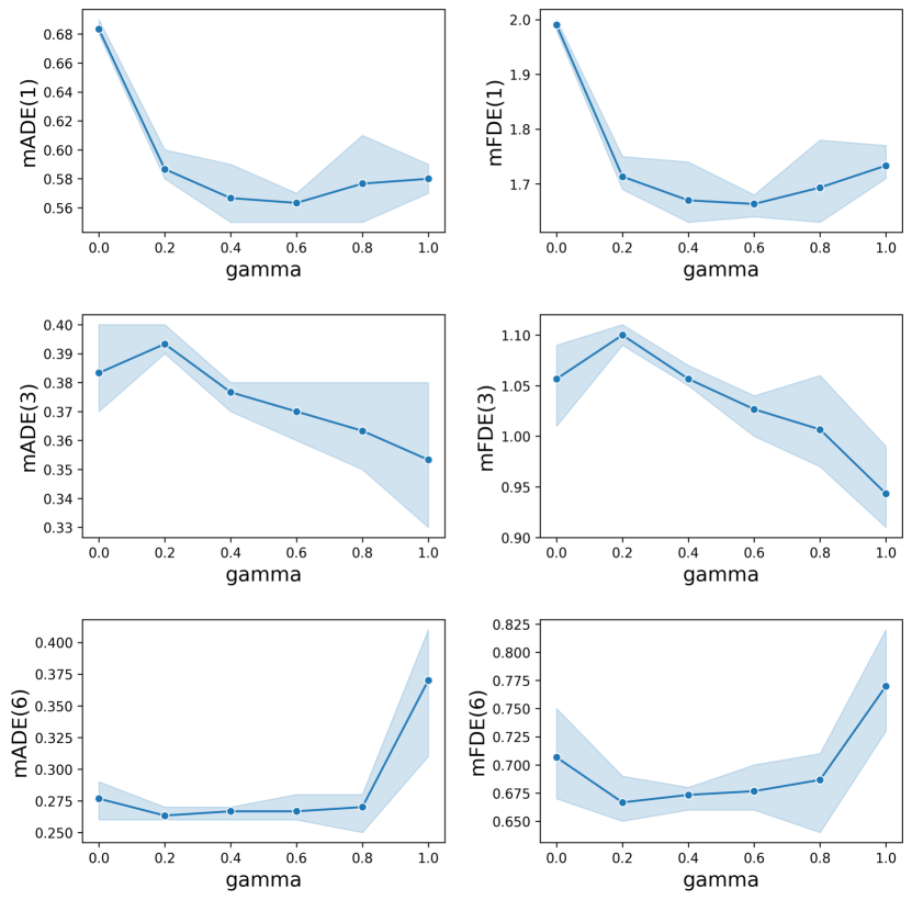
Figure 5: Sensitivity analysis on $\gamma$ (gamma) using AutoBots backbone on the Interaction dataset.

This section showcases the effect of $\gamma$ on our HWTA loss $\mathcal{L}$. In particular, Fig. 5 illustrates the variation of performance for different $\gamma$ values. Note that for $\gamma=0.0$ the meta-mode loss $\mathcal{L}_{\text{meta}}$ is not used and for $\gamma=1.0$ the loss $\mathcal{L}_{\text{MWTA}}$ is annealed. From our experiments, $\mathcal{L}_{\text{meta}}$ is necessary for better accuracy on most confident predictions as we observe a dramatic decrease in $\text{mADE}_{1}$ and $\text{mFDE}_{1}$

Appendix 0.E Importance of the Width Factor

Table 6: Performance of HLT-Ens - ADAPT (averaged over three runs) on Interaction wrt. $\boldsymbol{\alpha}$. Our ensemble has $M=4$ subnetworks, with $K=2$ meta-modes containing $K^{\prime}=3$ modes each.

$\boldsymbol{\alpha}$ value	$\text{mADE}_{1}$ $\downarrow$	$\text{mFDE}_{1}$ $\downarrow$	$\text{mADE}_{6}$ $\downarrow$	$\text{mFDE}_{6}$ $\downarrow$	#Prm (M)
1	0.78	2.24	0.45	1.18	0.4
2	0.61	1.79	0.34	0.87	1.5
3	0.55	1.58	0.28	0.69	3.1
4	0.51	1.48	0.25	0.62	5.5

Table 7: Performance of HLT-Ens - ADAPT (averaged over three runs) on Interaction wrt. $\boldsymbol{\alpha}$. Our ensemble has $M=8$ subnetworks, with $K=2$ meta-modes containing $K^{\prime}=3$ modes each.

$\boldsymbol{\alpha}$ value	$\text{mADE}_{1}$ $\downarrow$	$\text{mFDE}_{1}$ $\downarrow$	$\text{mADE}_{6}$ $\downarrow$	$\text{mFDE}_{6}$ $\downarrow$	#Prm (M)
3	0.62	1.82	0.36	0.93	1.7
4	0.59	1.71	0.32	0.82	2.9
6	0.53	1.53	0.27	0.69	6.3
8	0.51	1.47	0.26	0.65	10.9

Our efficient ensembling architecture depends on two hyperparameters. $M$ corresponds to the ensemble size, and $\alpha$, as a factor on the embedding size, controls the width of the DNN. We evaluate the sensitivity of HLT-Ens to these parameters by training models using ADAPT backbone on the Interaction dataset with various settings. Tab. 6 and Tab. 7 showcase the effect of $\alpha$ for $4$ and $8$ subnetworks respectively. Increasing $\alpha$ enables better results until it reaches a plateau at a cost of more parameters.

Appendix 0.F Robustness Analysis over Mode Number

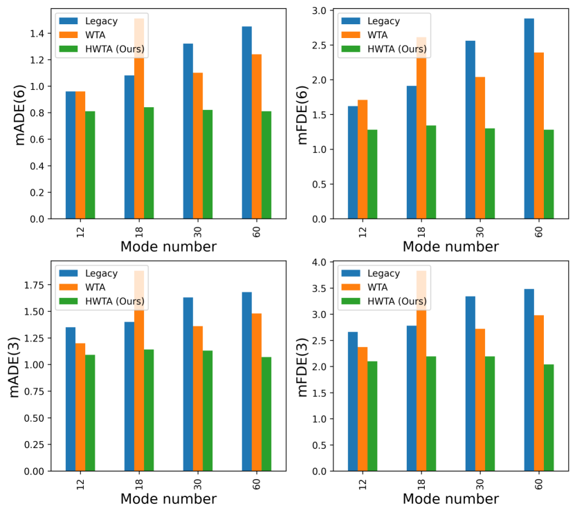
Figure 6: Performance comparison under variations of the number of modes. We train three AutoBots using the Legacy loss, the WTA loss, and the HWTA loss on Argoverse 1. We report their performance in terms of $\text{mADE}_{3}$, $\text{mFDE}_{3}$, $\text{mADE}_{6}$ and $\text{mFDE}_{6}$. For our loss, we considered $6$ meta-modes.

The number of modes is a critical hyperparameter significantly impacting the model’s performance. To cover the true multimodal distribution it is often preferred to predict more modes and choose subsequently the most confident ones. Yet, doing so might decrease the diversity in the predicted modes as the most confident mode is likely to have duplicates. Using hierarchy in the mixture distribution, we showcase that we are able to reduce our mixture complexity while retaining most of its diversity. Fig. 6 illustrates the impact of the number of modes over the performance on diversity metrics (i.e., $\text{mADE}_{6}$ and $\text{mFDE}_{6}$). The comparison is done with three different settings (Legacy loss, WTA loss, and HWTA loss) all using AutoBots backbone and trained on Argoverse 1. Concerning our loss, instead of taking the $6$ most confident trajectories, we directly use the $6$ meta-modes as a set of forecasts. Doing so seems to stabilize the performance, suggesting our loss enables more robustness to variations in the number of modes with a fixed number of meta-modes.

Appendix 0.G Diversity in Ensembles of Mixtures

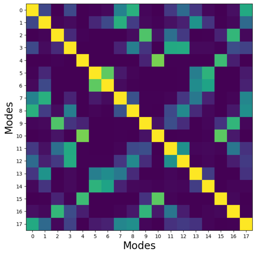
(a) DE similarity matrix

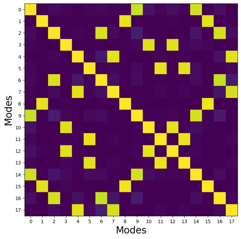
(b) HLT-Ens similarity matrix

Figure 7: Similarity matrices for DE and HLT-Ens on Argoverse 1. We use the AutoBots backbone, to construct ensembles of size $M=3$. For HLT-Ens, we set $\alpha=1.5$.

Prediction diversity is essential for the performance of ensembles. In [22], the authors present two sources of stochasticity in the training process producing diversity among ensemble members: the random initialization of the model’s parameters and the shuffling of the batches. HLT-Ens does not benefit from this last source of stochasticity, yet has comparable performance. To provide more insight into the effect on the diversity of this source of stochasticity in the training of trajectory forecasting models, we conducted a small experiment on the consistency of the cluster found by the post-hoc KMeans algorithm on our ensembles.Fig. 7 presents the similarity matrices for both DE and HLT-Ens. Each cell represents the rate of two modes being clusterized in the same cluster by the KMeans algorithm on the validation set of Argoverse 1. It appears that the clustering is more consistent for HLT-Ens highlighting the possibility to cluster only once the modes and apply it after without too much performance loss compared to executing a KMeans algorithm for each sample.

Appendix 0.H SceneTransformer Experiments

Table 8: Performance comparison on Interaction using SceneTransformer backbone. All ensembles have $M=3$ subnetworks and are followed by a KMeans algorithm to form $6$ trajectory clusters from which we take the centroids; we highlight the best performances in bold. For our method, we consider $\alpha=1.5$. The number of parameters is expressed in millions. M.A. corresponds to the inference cost, i.e., the number of Mega multiply-add operations for a forward pass, which is estimated with the python package torchinfo [39].

	Method	$\text{mADE}_{1}$ $\downarrow$	$\text{mADE}_{3}$ $\downarrow$	$\text{mADE}_{6}$ $\downarrow$	$\text{mFDE}_{1}$ $\downarrow$	$\text{mFDE}_{3}$ $\downarrow$	$\text{mFDE}_{6}$ $\downarrow$	$\text{NLL}_{3}$ $\downarrow$	$\text{NLL}_{6}$ $\downarrow$	#Prm $\downarrow$
Single	Single model
	Legacy	0.66	0.31	0.21	1.50	0.66	0.39	18.57	17.23
	HWTA (Ours)	0.48	0.32	0.26	1.17	0.71	0.52	-4.74	-11.15	11.8
	Ensemble
	DE	0.57	0.28	0.21	1.30	0.60	0.39	23.09	22.59	35.4
	HT-Ens (Ours)	0.50	0.32	0.23	1.19	0.69	0.47	-7.34	-9.94	35.4
	HLT-Ens (Ours)	0.49	0.32	0.25	1.17	0.72	0.53	-4.24	-9.59	8.9

Tab. 8 presents the performance of our method on the SceneTransformer backbone trained on the Interaction dataset. These results are based on a custom re-implementation of SceneTransformer we developed. These preliminary results showcase the ability of our approach to improve the most confident forecast accuracy as well as the quality of the predicted multimodal distribution compared to the original loss of SceneTransformer. However, it seems to lack diversity in the predicted modes. We argue it might be necessary to try out other values of $\gamma$ (we used $\gamma=0.6$ here).

References

- [1] Aydemir, G., Akan, A.K., Güney, F.: Adapt: Efficient multi-agent trajectory prediction with adaptation. In: ICCV (2023)
- [2] Ba, J.L., Kiros, J.R., Hinton, G.E.: Layer normalization. arXiv preprint arXiv:1607.06450 (2016)
- [3] Bahari, M., Nejjar, I., Alahi, A.: Injecting knowledge in data-driven vehicle trajectory predictors. Transportation research part C: emerging technologies (2021)
- [4] Bengler, K., Dietmayer, K., Farber, B., Maurer, M., Stiller, C., Winner, H.: Three decades of driver assistance systems: Review and future perspectives. IEEE Intelligent transportation systems magazine (2014)
- [5] Bishop, C.M.: Mixture density networks (1994)
- [6] Caesar, H., Bankiti, V., Lang, A.H., Vora, S., Liong, V.E., Xu, Q., Krishnan, A., Pan, Y., Baldan, G., Beijbom, O.: nuscenes: A multimodal dataset for autonomous driving. In: CVPR (2020)
- [7] Chai, Y., Sapp, B., Bansal, M., Anguelov, D.: Multipath: Multiple probabilistic anchor trajectory hypotheses for behavior prediction. In: CoRL (2020)
- [8] Chang, M.F., Lambert, J., Sangkloy, P., Singh, J., Bak, S., Hartnett, A., Wang, D., Carr, P., Lucey, S., Ramanan, D., et al.: Argoverse: 3d tracking and forecasting with rich maps. In: ICCV (2019)
- [9] Cui, H., Radosavljevic, V., Chou, F.C., Lin, T.H., Nguyen, T., Huang, T.K., Schneider, J., Djuric, N.: Multimodal trajectory predictions for autonomous driving using deep convolutional networks. In: ICRA (2019)
- [10] Deo, N., Trivedi, M.M.: Convolutional social pooling for vehicle trajectory prediction. In: CVPR Workshops (2018)
- [11] Deo, N., Trivedi, M.M.: Multi-modal trajectory prediction of surrounding vehicles with maneuver based lstms. In: IV (2018)
- [12] Frankle, J., Carbin, M.: The lottery ticket hypothesis: Finding sparse, trainable neural networks. ICLR (2019)
- [13] Girgis, R., Golemo, F., Codevilla, F., Weiss, M., D’Souza, J.A., Kahou, S.E., Heide, F., Pal, C.: Latent variable sequential set transformers for joint multi-agent motion prediction. ICLR (2022)
- [14] Guo, C., Pleiss, G., Sun, Y., Weinberger, K.Q.: On calibration of modern neural networks. In: ICML (2017)
- [15] Gupta, A., Johnson, J., Fei-Fei, L., Savarese, S., Alahi, A.: Social gan: Socially acceptable trajectories with generative adversarial networks. In: CVPR (2018)
- [16] Guzman-Rivera, A., Batra, D., Kohli, P.: Multiple choice learning: Learning to produce multiple structured outputs. NeurIPS (2012)
- [17] Havasi, M., Jenatton, R., Fort, S., Liu, J.Z., Snoek, J., Lakshminarayanan, B., Dai, A.M., Tran, D.: Training independent subnetworks for robust prediction. In: ICLR (2021)
- [18] Ivanovic, B., Pavone, M.: The trajectron: Probabilistic multi-agent trajectory modeling with dynamic spatiotemporal graphs. In: ICCV (2019)
- [19] Izmailov, P., Podoprikhin, D., Garipov, T., Vetrov, D., Wilson, A.G.: Averaging weights leads to wider optima and better generalization. arXiv preprint arXiv:1803.05407 (2018)
- [20] Krizhevsky, A., Sutskever, I., Hinton, G.E.: Imagenet classification with deep convolutional neural networks. NeurIPS (2012)
- [21] Lakshminarayanan, B., Pritzel, A., Blundell, C.: Simple and scalable predictive uncertainty estimation using deep ensembles. NeurIPS (2017)
- [22] Laurent, O., Lafage, A., Tartaglione, E., Daniel, G., Martinez, J.M., Bursuc, A., Franchi, G.: Packed-ensembles for efficient uncertainty estimation. ICLR (2023)
- [23] Lee, N., Choi, W., Vernaza, P., Choy, C.B., Torr, P.H.S., Chandraker, M.: Desire: Distant future prediction in dynamic scenes with interacting agents. In: CVPR (2017)
- [24] Lee, S., Purushwalkam, S., Cogswell, M., Crandall, D., Batra, D.: Why m heads are better than one: Training a diverse ensemble of deep networks. arXiv preprint arXiv:1511.06314 (2015)
- [25] Lee, S., Purushwalkam Shiva Prakash, S., Cogswell, M., Ranjan, V., Crandall, D., Batra, D.: Stochastic multiple choice learning for training diverse deep ensembles. NeurIPS (2016)
- [26] Lefèvre, S., Vasquez, D., Christian, L.: A survey on motion prediction and risk assessment for intelligent vehicles. In: ROBOMECH Journal (2014)
- [27] Ma, H., Li, J., Zhan, W., Tomizuka, M.: Wasserstein generative learning with kinematic constraints for probabilistic interactive driving behavior prediction. In: IV (2019)
- [28] Makansi, O., Ilg, E., Cicek, O., Brox, T.: Overcoming limitations of mixture density networks: A sampling and fitting framework for multimodal future prediction. In: CVPR (2019)
- [29] Mangalam, K., Girase, H., Agarwal, S., Lee, K.H., Adeli, E., Malik, J., Gaidon, A.: It is not the journey but the destination: Endpoint conditioned trajectory prediction. In: Vedaldi, A., Bischof, H., Brox, T., Frahm, J.M. (eds.) ECCV (2020)
- [30] McAllister, R., Gal, Y., Kendall, A., Van Der Wilk, M., Shah, A., Cipolla, R., Weller, A.: Concrete problems for autonomous vehicle safety: Advantages of bayesian deep learning. In: IJCAI (2017)
- [31] Mercat, J., Gilles, T., El Zoghby, N., Sandou, G., Beauvois, D., Gil, G.P.: Multi-head attention for multi-modal joint vehicle motion forecasting. In: ICRA (2020)
- [32] Nayakanti, N., Al-Rfou, R., Zhou, A., Goel, K., Refaat, K.S., Sapp, B.: Wayformer: Motion forecasting via simple & efficient attention networks. In: ICRA (2023)
- [33] Ngiam, J., Caine, B., Vasudevan, V., Zhang, Z., Chiang, H.T.L., Ling, J., Roelofs, R., Bewley, A., Liu, C., Venugopal, A., et al.: Scene transformer: A unified architecture for predicting multiple agent trajectories. In: ICLR (2022)
- [34] Nguyen, A., Yosinski, J., Clune, J.: Deep neural networks are easily fooled: High confidence predictions for unrecognizable images. In: CVPR (2015)
- [35] Rupprecht, C., Laina, I., DiPietro, R., Baust, M., Tombari, F., Navab, N., Hager, G.D.: Learning in an uncertain world: Representing ambiguity through multiple hypotheses. In: ICCV (2017)
- [36] Salzmann, T., Ivanovic, B., Chakravarty, P., Pavone, M.: Trajectron++: Dynamically-feasible trajectory forecasting with heterogeneous data. In: ECCV (2020)
- [37] Schreier, M., Willert, V., Adamy, J.: An integrated approach to maneuver-based trajectory prediction and criticality assessment in arbitrary road environments. IEEE Transactions on Intelligent Transportation Systems (2016)
- [38] Tang, C., Salakhutdinov, R.R.: Multiple futures prediction. In: NeurIPS (2019)
- [39] Torchinfo: Torchinfo. https://github.com/TylerYep/torchinfo (2022), version: 1.7.1
- [40] Varadarajan, B., Hefny, A., Srivastava, A., Refaat, K.S., Nayakanti, N., Cornman, A., Chen, K., Douillard, B., Lam, C.P., Anguelov, D., et al.: Multipath++: Efficient information fusion and trajectory aggregation for behavior prediction. In: ICRA (2022)
- [41] Vaswani, A., Shazeer, N., Parmar, N., Uszkoreit, J., Jones, L., Gomez, A.N., Kaiser, Ł., Polosukhin, I.: Attention is all you need. NeurIPS (2017)
- [42] Wang, Y., Zhou, H., Zhang, Z., Feng, C., Lin, H., Gao, C., Tang, Y., Zhao, Z., Zhang, S., Guo, J., et al.: Tenet: Transformer encoding network for effective temporal flow on motion prediction. arXiv preprint arXiv:2207.00170 (2022)
- [43] Wen, Y., Tran, D., Ba, J.: BatchEnsemble: an alternative approach to efficient ensemble and lifelong learning. In: ICLR (2019)
- [44] Wilson, B., Qi, W., Agarwal, T., Lambert, J., Singh, J., Khandelwal, S., Pan, B., Kumar, R., Hartnett, A., Pontes, J.K., et al.: Argoverse 2: Next generation datasets for self-driving perception and forecasting. NeurIPS Datasets and Benchmarks (2021)
- [45] Wu, Y., He, K.: Group normalization. In: ECCV (2018)
- [46] Xie, S., Girshick, R., Dollár, P., Tu, Z., He, K.: Aggregated residual transformations for deep neural networks. In: CVPR (2017)
- [47] Yuan, Y., Weng, X., Ou, Y., Kitani, K.M.: Agentformer: Agent-aware transformers for socio-temporal multi-agent forecasting. In: ICCV (2021)
- [48] Zhan, W., Sun, L., Wang, D., Shi, H., Clausse, A., Naumann, M., Kummerle, J., Konigshof, H., Stiller, C., de La Fortelle, A., et al.: Interaction dataset: An international, adversarial and cooperative motion dataset in interactive driving scenarios with semantic maps. arXiv preprint arXiv:1910.03088 (2019)
- [49] Zhou, Z., Wang, J., Li, Y.H., Huang, Y.K.: Query-centric trajectory prediction. In: CVPR (2023)
- [50] Zhou, Z., Ye, L., Wang, J., Wu, K., Lu, K.: Hivt: Hierarchical vector transformer for multi-agent motion prediction. In: CVPR (2022)