Chattering Phenomena in Time-Optimal Control for High-Order Chain-of-Integrators Systems with Full State Constraints

Abstract

Time-optimal control for high-order chain-of-integrators systems with full state constraints remains an open and challenging problem in the optimal control theory domain. The behaviors of optimal control in high-order problems lack precision characterization, even where the existence of the chattering phenomenon remains unknown and overlooked. This paper establishes a theoretical framework for chattering phenomena in the considered problem, providing novel findings on the uniqueness of state constraints inducing chattering, the upper bound on switching times in an unconstrained arc during chattering, and the convergence of states and costates to the chattering limit point. For the first time, this paper proves the existence of the chattering phenomenon in the considered problem. The chattering optimal control for 4th order problems with velocity constraints is precisely solved, providing an approach to plan strictly time-optimal snap-limited trajectories. Other cases of order $n\leq 4$ are proved not to allow chattering. The conclusions correct the longstanding misconception in the industry regarding the time-optimality of S-shaped trajectories with minimal switching times.

I Introduction

Time-optimal control for high-order chain-of-integrators systems with full state constraints is a classical problem in the optimal control theory domain and a fundamental problem within the field of kinematics, yet to be resolved. With time-optimal orientations and safety constraints, control for high-order chain-of-integrators systems has achieved universal application in computer numerical control machining [1], robotic motion control [2, 3, 4], semiconductor device fabrication [5], and autonomous driving [6]. However, the control’s behaviors in this issue have yet to be thoroughly investigated. For example, the existence of the chattering phenomenon [7] in the above problem is yet to be discovered, let alone the fully analysis on optimal control.

Formally, the investigated problem is described in (1a), where ${\boldsymbol{x}}=\left(x_{k}\right)_{k=1}^{n}\in{\mathbb{R}}^{n}$ is the state vector, $u\in{\mathbb{R}}$ is the control, and the terminal time ${t_{\mathrm{f}}}$ is free. ${\boldsymbol{x}}_{0}=\left(x_{0,k}\right)_{k=1}^{n}$ and ${\boldsymbol{x}}_{\mathrm{f}}=\left(x_{{\mathrm{f}}k}\right)_{k=1}^{n}$ are the assigned initial state vector and terminal state vector. $n$ is the order of problem (1a). ${\boldsymbol{M}}=\left(M_{k}\right)_{k=0}^{n}\in{\mathbb{R}}_{++}\times\overline{{\mathbb{R}}}_{++}^{n}$, where $\overline{{\mathbb{R}}}_{++}={\mathbb{R}}_{++}\cup\left\{\infty\right\}$ is the strictly positive part of the extended real number line. The notation $\left(\bullet\right)$ means $\left[\bullet\right]^{\top}$. Problem (1a) possesses a clear physical significance. For instance, if $n=4$, $x_{4}$, $x_{3}$, $x_{2}$, $x_{1}$, and $u$ respectively refer to the position, velocity, acceleration, jerk, and snap of a 1-axis motion system. In this case, (1a) requires a trajectory with minimum motion time from a given initial state vector to a terminal state vector under box constraints.

$$\min\quad J=\int_{0}^{{t_{\mathrm{f}}}}\mathrm{d}t={t_{\mathrm{f}}},$$ (1a)

$${\mathrm{s.t.}}\quad \dot{x}_{k}\left(t\right)=x_{k-1}\left(t\right),\,\forall 1<k\leq n,\,t\in\left[0,t_{\mathrm{f}}\right],$$ (1b)

$$\dot{x}_{1}\left(t\right)=u\left(t\right),\,\forall t\in\left[0,t_{\mathrm{f}}\right],$$ (1c)

$${\boldsymbol{x}}\left(0\right)={\boldsymbol{x}}_{0},\,{\boldsymbol{x}}\left({t_{\mathrm{f}}}\right)={\boldsymbol{x}}_{\mathrm{f}},$$ (1d)

$$\left|x_{k}\left(t\right)\right|\leq M_{k},\,\forall 1\leq k\leq n,\,t\in\left[0,t_{\mathrm{f}}\right],$$ (1e)

$$\left|u\left(t\right)\right|\leq M_{0},\,\forall t\in\left[0,t_{\mathrm{f}}\right],$$ (1f)

Numerous studies have been conducted on problem (1a) from the perspectives of optimal control and model-based classification discourse. Problem (1a) without state constraints, i.e., $\forall 1\leq k\leq n$, $M_{k}=\infty$, can be fully solved by Pontryagin’s maximum principle (PMP) [8], where the analytic expression of the optimal control [9] is well-known. Once state constraints are introduced, problem (1a) becomes practically significant but challenging to solve. The 1st order and 2nd order problems are trivial [10]. After extensive exploration, the third-order problem has gradually been resolved. Haschke et al. [11] solved the 3rd order problem where $x_{{\mathrm{f}}2}=x_{{\mathrm{f}}3}=0$. Kröger [12] developed the Reflexxes library, solving 3rd order problems where $x_{{\mathrm{f}}3}=0$. Berscheid and Kröger[13] fully solved 3rd order problems without position constraints, i.e., $M_{3}=\infty$, resulting in the Ruckig library. Our previous work [14] completely solved 3rd order problems and fully enumerated the system behaviors for higher-order problems except the limit point of chattering. However, there exist no methods solving optimal solutions for 4th order or higher-order problems with full state constraints and arbitrary terminal states, despite the universal application of snap-limited trajectories for lithography machines and ultra-precision wafer stages with time-optimal orientations [15]. Specifically, even the existence of chattering in problem (1a) remains unsolved, let alone a comprehensive understanding of the optimal control.

Figure 1: (a-d) Strictly optimal trajectories for position-to-position problems of order $n=1,2,3,4$, respectively. (e) A suboptimal trajectory for the same 4th order problem to (d) planned by the MIM method in our previous work [14]. (f) Augmented switching laws of trajectories in (d-e). In (a-e), the upper figures show the states, the lower figures show the costates, and the numerical sequences represent the augmented switching laws. $M_{0}=1$, $M_{1}=1$, $M_{2}=1.5$, $M_{3}=4$, $M_{4}=15$. For an $n$-th order problem, ${\boldsymbol{x}}_{0}=-M_{n}{\boldsymbol{e}}_{n}$, ${\boldsymbol{x}}_{\mathrm{f}}=M_{n}{\boldsymbol{e}}_{n}$. In (a-e), $\bar{u}=\frac{u}{M_{0}}$. $\forall 1\leq k\leq 4$, $\bar{x}_{k}=\frac{x_{k}}{M_{k}}$, and $\bar{\lambda}_{k}=\frac{\lambda_{k}}{\left\|\lambda_{k}\right\|_{\infty}}$. (d3-d4) show the enlargements of (d1-d2) during the chattering period. The abscissa is in logarithmic scale with respect to time, i.e., $-\log_{10}\left(t_{\infty}-t\right)$, where $t_{\infty}\approx 6.0732$ is the first chattering limit time. $\forall k=1,2,3$, $\hat{x}_{k}\left(t\right)=\frac{x_{k}^{*}\left(t\right)\left(t_{\infty}-t\right)^{-k}}{\left\|x_{k}^{*}\left(t\right)\left(t_{\infty}-t\right)^{-k}\right\|_{\infty}}$, and $\hat{\lambda}_{k}\left(t\right)=\frac{\lambda_{k}\left(t\right)\left(t_{\infty}-t\right)^{k-4}}{\left\|\lambda_{k}\left(t\right)\left(t_{\infty}-t\right)^{k-4}\right\|_{\infty}}$.

Generally, the chattering phenomenon [7] represents a gap to investigate and numerically solve high-order optimal control problems with inequality state constraints. In the optimal control theory domain, chattering means that the optimal control switches for infinitely many times in a finite time period [16]. Fuller [17] found the first optimal control problem with chattering arcs, fully studying a problem for the 2nd order chain-of-integrators system with minimum energy. Robbins [18] constructed a 3rd order chain-of-integrators system whose optimal control is chattering with a finite total variation. Chattering in hybrid systems is investigated as Zeno phenomenon [19, 20]. Kupka [21] proved the ubiquity of the chattering phenomenon, i.e., optimal control problems with a Hamiltonian affine in the single input control and a chattering optimal control constitutes an open semialgebraic set. Numerous problems in the industry have been found to have optimal solutions with chattering [22, 23], where the chattering phenomenon impedes the theoretical analysis and numerical computation of optimal control. Among them, little research has been conducted on the existence of the chattering phenomenon in the classical problem (1a). Neither proofs on non-existence nor counterexamples to the chattering phenomenon in problem (1a) have existed so far. In practice, there exists a longstanding oversight of the chattering phenomenon in problem (1a) regarding the time-optimality of S-shaped trajectories with minimum switching times, where some works even tried to minimize terminal time by reducing switching times of control [24, 25]. As shown in Fig. 1(a-c), time-optimal trajectories of order $n\leq 3$ exhibit a recursively nested S-shaped form. Hence, it is intuitively plausible to expect 4th order optimal trajectories to possess a form in Fig. 1(e). However, as proved in Section V, chattering phenomena occur in 4th order trajectories. The optimal trajectory of 4th order is shown in Fig. 1(d).

Geometric control theory represents a significant mathematical tool to investigate the mechanism underlying chattering [26]. As judged in [27], Zelikin and Borisov [7] have achieved the most comprehensive treatment of the chattering phenomenon so far. In [7], the order of a singular trajectory is defined based on the Poisson bracket of Hamiltonian affine in control, while 2nd order problems with chattering were fully discussed based on designing Lagrangian manifolds. However, although problem (1a) has a Hamiltonian affine in control, the order of singular trajectories in problem (1a) is undetermined since any order derivatives of the costates do not explicitly involve the control $u$. As a result, the chattering phenomenon in problem (1a) remains challenging to investigate.

It is meaningful to address impediment on numerical computation from the chattering nature of optimal control. Zelikin and Borisov [28] reasoned that discontinuity induced by chattering worsens the approximation in numerical integration methods, thus obstructing the application of shooting methods in optimal control. Laurent et al. [29] proposed an interior-point approach to solve optimal control problems, where chattering phenomena worsen the convergence of the algorithm. Caponigro et al. [30] proposed a regularization method by adding a penalization of the total variation to suppress the chattering phenomenon, successfully obtaining quasi-optimal solutions without chattering. However, it is challenging to prove the existence of chattering for a numerical solution due to the limited precision of numerical computation.

Based on the theoretical framework built in our previous work [14], this paper theoretically investigated chattering phenomena in the open problem (1a), i.e., time-optimal control for high-order chain-of-integrators systems with full state constraints. Section II formulates problem (1a) by Hamiltonian and introduces some results of [14] as preliminaries. Section III derives necessary conditions for chattering phenomena in problem (1a). Section IV and Section V prove that velocity constraints can induce chattering in 4th order problems, while other cases of order $n\leq 4$ do not allow chattering. The contribution of this paper is as follows.

1. This paper establishes a theoretical framework for the chattering phenomenon in the classical and open problem (1a) in the optimal control theory domain, i.e., time-optimal control for high-order chain-of-integrators systems with full state constraints. The framework provides novel findings on the existence of chattering, the uniqueness of state constraints inducing chattering, the upper bound on switching times in every unconstrained arc during chattering, and the convergence of states as well as costates to the chattering limit point. Existing works [11, 12, 13] lack precise characterization of optimal control’s behaviors in the high-order problem. Even the existence of the chattering phenomenon remains unknown and overlooked. Since any order derivatives of costates are independent of the input control, the predominant technology for chattering analysis based on Lagrangian manifolds [7] is difficult to directly apply to the investigated problem, which demonstrates the necessity and significance of the established framework for problem (1a).

2. Based on the developed theory, this paper proves that chattering phenomena do not exist in problems of order $n\leq 3$, and 4th order problems without velocity constraints. For any $n$-th order problems, state constraints on $x_{n}$ and $x_{1}$ are proved unable to induce chattering. Furthermore, constrained arcs with positive lengths cannot occur during chattering periods.

3. To the best of our knowledge, this paper proves the existence of chattering in problem (1a) for the first time, correcting the longstanding misconception in the industry regarding the time-optimality of S-shaped trajectories with minimal switching times. This paper proves that 4th order problems with velocity constraints can induce chattering, where the decay rate in the time domain is precisely solved as $\alpha^{*}\approx 0.1660687$. Hence, chattering can occur in higher-order problems as well. For the first time, time-optimal snap-limited trajectories with full state constraints can be planned based on the developed theory. The chattering control is applicable in practice due to the finite control frequency. Note that snap-limited position-to-position trajectories are universally applied for ultra-precision control in the industry, while the overlooking of chattering impedes the approach to time-optimal profiles in previous works [25].

II Preliminaries

This section represents preliminaries before discussing chattering phenomena in problem (1a). Section II-A formulates problem (1a) with analysis on Hamiltonian. Section II-B introduces some results of our previous work [14].

II-A Problem Formulation

This section formulates the optimal control problem (1a) from the perspective of Hamiltonian. The Hamiltonian is

$${\mathcal{H}}\left({\boldsymbol{x}}\left(t\right),u\left(t\right),\lambda_{0},{\boldsymbol{\lambda}}\left(t\right),{\boldsymbol{\eta}}\left(t\right),t\right)$$ (2)

$$= \lambda_{0}+\lambda_{1}u+\sum_{k=2}^{n}\lambda_{k}x_{k-1}+\sum_{k=1}^{n}\eta_{k}\left(\left|x_{k}\right|-M_{k}\right),$$

where $\lambda_{0}\geq 0$ is a constant. ${\boldsymbol{\lambda}}\left(t\right)=\left(\lambda_{k}\left(t\right)\right)_{k=1}^{n}$ is the costate vector. $\lambda_{0}$ and ${\boldsymbol{\lambda}}$ satisfy $\left(\lambda_{0},{\boldsymbol{\lambda}}\left(t\right)\right)\not=0$. The initial costates ${\boldsymbol{\lambda}}\left(0\right)$ and the terminal costates ${\boldsymbol{\lambda}}\left({t_{\mathrm{f}}}\right)$ are not assigned since ${\boldsymbol{x}}\left(0\right)$ and ${\boldsymbol{x}}\left({t_{\mathrm{f}}}\right)$ are given in problem (1a).

${\boldsymbol{\lambda}}$ satisfies the Euler-Lagrange equations [31], i.e.,

$$\dot{\lambda}_{k}=-\frac{\partial{\mathcal{H}}}{\partial x_{k}},\,\forall 1\leq k\leq n.$$ (3)

By (2), it holds that

$$\begin{dcases}\dot{\lambda}_{k}=-\lambda_{k+1}-\eta_{k}\,{\mathrm{sgn}}\left(x_{k}\right),\,\forall 1\leq k<n,\\ \dot{\lambda}_{n}=-\eta_{n}\,{\mathrm{sgn}}\left(x_{n}\right).\end{dcases}$$ (4)

In (2), ${\boldsymbol{\eta}}$ is the multiplier vector induced by inequality state constraints (1e), satisfying

$$\eta_{k}\geq 0,\,\eta_{k}\left(\left|x_{k}\right|-M_{k}\right)=0,\,\forall 1\leq k\leq n.$$ (5)

Equivalently, $\forall t\in\left[0,t_{\mathrm{f}}\right]$, $\eta_{k}\left(t\right)\not=0$ only if $\left|x_{k}\left(t\right)\right|=M_{k}$.

Note that $\left|x_{n}\right|\equiv M_{n}$ for a time period contradicts the time-optimality. Hence, $\left|x_{n}\right|<M_{n}$ almost everywhere. The term “almost everywhere” means a property holds except for a zero-measure set [32]. By (4) and (5), it holds that

$$\eta_{n}=0,\,\dot{\lambda}_{n}=0\text{ almost everywhere}.$$ (6)

PMP [8] states that the input control $u\left(t\right)$ minimizes the Hamiltonian ${\mathcal{H}}$ in the feasible set, i.e.,

$$u\left(t\right)\in\mathop{\arg\min}\limits_{\left|U\right|\leq M_{0}}{\mathcal{H}}\left({\boldsymbol{x}}\left(t\right),U,\lambda_{0},{\boldsymbol{\lambda}}\left(t\right),{\boldsymbol{\eta}}\left(t\right),t\right).$$ (7)

Hence, a Bang-Singular-Bang control law [14] is induced as

$$u\left(t\right)=\begin{dcases}M_{0},&\lambda_{1}\left(t\right)<0\\ *,&\lambda_{1}\left(t\right)=0\\ -M_{0},&\lambda_{1}\left(t\right)>0\end{dcases},$$ (8)

where $u\left(t\right)\in\left[-M_{0},M_{0}\right]$ is undetermined during $\lambda_{1}\left(t\right)=0$.

Note that the objective function $J=\int_{0}^{{t_{\mathrm{f}}}}\mathrm{d}t$ is in a Lagrangian form; hence, the continuity of the system is guaranteed by the following equality, i.e.,

$$\forall t\in\left[0,t_{\mathrm{f}}\right],\,{\mathcal{H}}\left({\boldsymbol{x}}\left(t\right),u\left(t\right),\lambda_{0},{\boldsymbol{\lambda}}\left(t\right),{\boldsymbol{\eta}}\left(t\right),t\right)\equiv 0.$$ (9)

(9) allows the junction of costates [8] when some inequality state constraints switch between active and inactive. Specifically, results in [8] imply the following proposition.

Proposition 1 (Junction condition in problem (1a)).

Junction of costates in problem (1a) can occur at $t_{1}$ if $\exists 1\leq k\leq n$, s.t. (a) $\left|x_{k}\right|$ is tangent to $M_{k}$, i.e., $\left|x_{k}\left(t_{1}\right)\right|=M_{k}$ and $\left|x_{k}\right|<M_{k}$ in a deleted neighborhood of $t_{1}$; or (b) the system enters or leaves the constrained arc $\left|x_{k}\right|\equiv M_{k}$, i.e., $\left|x_{k}\right|\equiv M_{k}$ at a one-sided neighborhood of $t_{1}$ and $\left|x_{k}\right|<M_{k}$ at another one-sided neighborhood of $t_{1}$. Specifically, $\exists\mu\leq 0$, s.t.

$${\boldsymbol{\lambda}}\left(t_{1}^{+}\right)-{\boldsymbol{\lambda}}\left(t_{1}^{-}\right)=\mu\frac{\partial\left(\left|x_{k}\right|-M_{k}\right)}{\partial{\boldsymbol{x}}}=\mu\,{\mathrm{sgn}}\left(x_{k}\right){\boldsymbol{e}}_{k}.$$ (10)

In other words, $\lambda_{k}\left(t_{1}^{+}\right)-\lambda_{k}\left(t_{1}^{-}\right)=\mu\,{\mathrm{sgn}}\left(x_{k}\right)$, while $\forall j\not=k$, $\lambda_{j}$ is continuous at $t_{1}$. Furthermore, a junction cannot occur during an unconstrained arc or a constrained arc.

Remark.

Proposition 1 allows ${\boldsymbol{\lambda}}$ to jump between an unconstrained arc and a constrained arc or between two unconstrained arcs at the constrained boundary. Junction of ${\boldsymbol{\lambda}}$ significantly enriches the behavior of optimal control in problem (1a), since (4), (5), and (8) determine an upper bound on control’s switching time. As will be reasoned in Section V, chattering phenomena in problem (1a) is induced by junction condition. Furthermore, ${\boldsymbol{x}}$ at the junction time determines the feasibility of a given trajectory. Therefore, the junction time is a key point along the optimal trajectory, which induces the system behavior and the tangent marker in Section II-B.

A 3rd order optimal trajectory is shown in Fig. 2 as an example. The Bang-Singular-Bang control law (8) can be verified in Fig. 2(a-b). (9) can be verified in Fig. 2(b). Junction of $\lambda_{3}$ occurs at $t_{3}$, since $x_{3}$ is tangent to $-M_{3}$ at $t_{3}$.

The system dynamics (1b) and (1c) are as follows.

Proposition 2 (System dynamics of problem (1a)).

Assume that $\forall 1\leq i\leq N$, $u\equiv u_{i}$ on $t\in\left(t_{i-1},t_{i}\right)$, where $\left\{t_{i}\right\}_{i=0}^{N}$ increases strictly monotonically. Then, $\forall 1\leq k\leq n$,

$$x_{k}\left(t_{N}\right)= \sum_{j=1}^{k}\frac{x_{k-j}\left(t_{0}\right)}{j!}t_{N}^{j}+\sum_{i=1}^{N}\frac{\Delta u_{i}}{k!}T_{i}^{k},$$ (11)

where $\Delta u_{i}=u_{i}-u_{i-1}$, $u_{0}=0$, and $T_{i}=t_{N}-t_{i-1}$.

Proof.

(11) holds for $x_{k}\left(t_{0}\right)$. Assume that (11) holds for $x_{k}\left(t_{N-1}\right)$. Then, (1b) and (1b) imply that

$$x_{k}\left(t_{N}\right)=\sum_{j=0}^{k}\frac{x_{k-j}\left(t_{N-1}\right)}{j!}T_{N}^{j},$$ (12)

where $x_{0}\left(t_{N-1}\right)\triangleq u_{N}$. It can be reasoned that (11) holds for $x_{k}\left(t_{N}\right)$. By induction, Proposition 2 holds. ∎

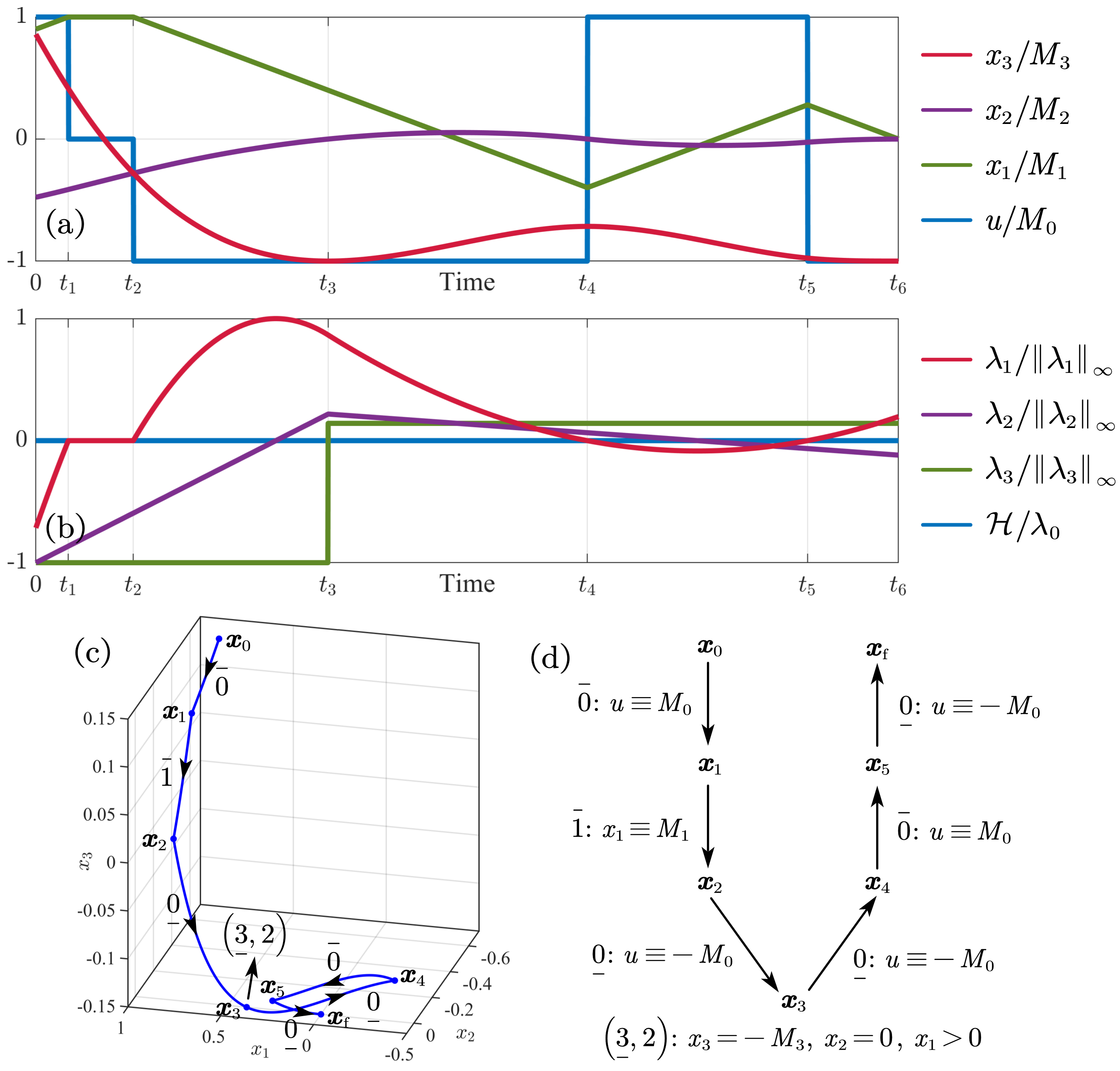
Figure 2: A 3rd order optimal trajectory planned by [14], whose augmented switching law is $S=\overline{01}\underline{0}\left(\underline{3},2\right)\underline{0}\overline{0}\underline{0}$. Among them, $\lambda_{0}>0$, ${\boldsymbol{x}}_{0}=\left(0.9,-0.715,0.1288\right)$, ${{\boldsymbol{x}}_{\mathrm{f}}}=\left(0,0,-0.15\right)$, and ${\boldsymbol{M}}=\left(1,1,1.5,0.15\right)$. (a) The state vector. (b) The costate vector. (c) The trajectory ${\boldsymbol{x}}={\boldsymbol{x}}\left(t\right)$. (d) The flow chat of $S$.

II-B Main Results of [14]

Based on the formulation in Section II-A, our previous work [14] developed a novel notation system and theoretical framework for problem (1a), where the augmented switching law is introduced as notations and behaviors of costates are summarized. A theorem in [14] fully provides behaviors of optimal control except chattering phenomena as follows.

Lemma 1 (Optimal Control’s Behavior [14]).

The following properties hold for the optimal control of problem (1a).

1. The optimal control is unique in an almost everywhere sense. In other words, if $u=u_{1}^{*}\left(t\right)$ and $u=u_{2}^{*}\left(t\right)$, $t\in\left[0,t_{\mathrm{f}}^{*}\right]$, are both optimal controls of (1a), then $u_{1}^{*}\left(t\right)=u_{2}^{*}\left(t\right)$ almost everywhere.

2. $u\left(t\right)=-{\mathrm{sgn}}\left(\lambda_{1}\left(t\right)\right)M_{0}$ almost everywhere. Specifically, $u\left(t\right)\equiv 0$ if $\lambda_{1}\left(t\right)\equiv 0$.

3. $\lambda_{1}$ is continuous despite the junction condition (10).

4. $\lambda_{k}$ consists of $\left(n-k\right)$-th degree polynomials and zero. Specifically, $\lambda_{k}\equiv 0$ if $\exists j\geq k$, $\left|x_{j}\right|\equiv M_{j}$.

5. If ${\boldsymbol{x}}$ enters $\left|x_{k}\right|\equiv M_{k}$ at $t_{1}$ from an unconstrained arc, then $u\left(t_{1}^{-}\right)=\left(-1\right)^{k-1}{\mathrm{sgn}}\left(x_{k}\left(t_{1}\right)\right)$. If ${\boldsymbol{x}}$ leaves $\left|x_{k}\right|\equiv M_{k}$ at $t_{1}$ and moves into an unconstrained arc, then $u\left(t_{1}^{+}\right)=-{\mathrm{sgn}}\left(x_{k}\left(t_{1}\right)\right)$.

6. If $\exists t_{1}\in\left(0,{t_{\mathrm{f}}}\right)$, s.t. $\left|x_{k}\right|$ is tangent to $M_{k}$ at $t_{1}$. Then, one and only one of the following conclusions hold:

   1. $\exists l<\frac{k}{2}$, s.t. $x_{k-1}=x_{k-2}=\dots=x_{k-2l+1}=0$ at $t_{1}$, while $x_{k-2l}\left(t_{1}\right)\not=0$, and ${\mathrm{sgn}}\left(x_{k-2l}\left(t_{1}\right)\right)=-{\mathrm{sgn}}\left(x_{k}\left(t_{1}\right)\right)$. Denote $h=2l$ as the degree of $\left|x_{k}\left(t_{1}\right)\right|=M_{k}$.

   2. $x_{k-1}=x_{k-2}=\dots=x_{1}=0$ at $t_{1}$. $u\left(t_{1}^{+}\right)=-\frac{M_{0}}{M_{k}}x_{k}\left(t_{1}\right)$, and $u\left(t_{1}^{-}\right)=\left(-1\right)^{k-1}\frac{M_{0}}{M_{k}}x_{k}\left(t_{1}\right)$. Denote $h=k$ as the degree of $\left|x_{k}\left(t_{1}\right)\right|=M_{k}$.

Denote the set $\mathcal{N}={\mathbb{N}}\times\left\{\pm 1\right\}$. $\forall s=\left(k,a\right)\in\mathcal{N}$, define the value of $s$ as $\left|s\right|=k$, and define the sign of $s$ as ${\mathrm{sgn}}\left(s\right)=a$. $\forall k\in{\mathbb{N}}$, denote $\left(k,1\right)$ and $\left(k,-1\right)$ as $\overline{k}$ and $\underline{k}$, respectively. For $s_{1},s_{2}\in\mathcal{N}$, denote $s_{1}=-s_{2}$ if $\left|s_{1}\right|=\left|s_{2}\right|$ and ${\mathrm{sgn}}\left(s_{1}\right)=-{\mathrm{sgn}}\left(s_{2}\right)$. Based on Lemma 1, the system behavior and the tangent marker in our previous work [14] are defined as follows.

Definition 1.

A system behavior $s\in\mathcal{N}$ of an unconstrained arc or a constrained arc in problem (1a) is denoted as follows:

1. Denote the arc where $u\equiv M_{0}\,\left(-M_{0}\right)$ as $s=\overline{0}\,\left(\underline{0}\right)$.

2. Denote the arc where $x_{k}\equiv M_{k}\,\left(-M_{k}\right)$ as $s=\overline{k}\,\left(\underline{k}\right)$.

Definition 2.

Assume $\left|x_{k}\right|$ is tangent to $M_{k}$ with a degree $h$ as described in Lemma 1-6. Then, the tangent marker is denoted as $\left(s,h\right)$, where $s\in\mathcal{N}$, $\left|s\right|=k$, and ${\mathrm{sgn}}\left(s\right)={\mathrm{sgn}}\left(x_{k}\left(t_{1}\right)\right)$.

Definition 3.

An augmented switching law $S=s_{1}s_{2}\dots s_{N}$ means that the optimal trajectory passes through $s_{1},s_{2},\dots,s_{N}$ sequentially, where $\forall 1\leq i\leq N$, $s_{i}$ is a system behavior or a tangent marker.

An example is shown in Fig. 2(c-d), where the optimal trajectory is represented as $S=\overline{01}\underline{0}\left(\underline{3},2\right)\underline{0}\overline{0}\underline{0}$. Firstly, the system passes through $u\equiv M_{0}$, $x_{1}\equiv M_{1}$, and $u\equiv-M_{0}$. Then, $x_{3}$ is tangent to $-M_{3}$ at $t_{3}$. Next, the system passes through $u\equiv-M_{0}$, $u\equiv M_{0}$, and $u\equiv-M_{0}$. Finally, ${\boldsymbol{x}}$ reaches ${{\boldsymbol{x}}_{\mathrm{f}}}$ at ${t_{\mathrm{f}}}$. It is noteworthy that the augmented switching law does not include the motion time of each stage, which is also necessary to determine the optimal control.

Based on the formulation in Section II-A and the main results of [14] in Section II-B, the chattering phenomenon in problem (1a) can be investigated in the following sections.

III Necessary Conditions for Chattering Phenomena in Problem (1a)

As pointed out in Section I, neither proofs on non-existence nor counterexamples to the chattering phenomenon in the classical problem (1a) have existed so far. The predominant technology for chattering analysis based on Lagrangian manifolds [7] is difficult to directly apply to (1a) for the following reasons. (2) implies that $H=H_{0}+H_{1}u$ is affine in $u$, where $H_{1}=\lambda_{1}$. By (4), $\forall i\in{\mathbb{N}}^{*}$, $\frac{\mathrm{d}^{i}H_{1}}{\mathrm{d}t^{i}}$ is independent of $u$; hence, even the order of $H_{1}$ is undetermined. Therefore, the technology in [7] is hard to directly apply to problem (1a).

In a chattering phenomenon, denote the limit time point as $t_{\infty}$, and assume chattering occurs in the left-side neighborhood of $t_{\infty}$. Then, $\forall\delta>0$, $\exists t_{\delta},t_{\delta}^{\prime}\in\left(t_{\infty}-\delta,t_{\infty}\right)$, $1\leq k\leq n$, s.t. $\left|x_{k}\left(t_{\delta}\right)\right|=M_{k}$, but $\left|x_{k}\left(t_{\delta}^{\prime}\right)\right|<M_{k}$. [18] points out that in chattering phenomena, the constrained arc joins the end of an infinite sequence of consecutive unconstrained arcs of finite total duration. Therefore, if the chattering phenomenon occurs in problem (1a), then $\exists\left\{t_{i}\right\}_{i=0}^{\infty}$ increasing monotonically and converging to $t_{\infty}$, s.t. $\forall i\in{\mathbb{N}}$, $\exists 1\leq k\leq n$, $\left|x_{k}\left(t_{i}\right)\right|=M_{k}$, but $\forall 1\leq k\leq n$, $\left|x_{k}\right|<M_{k}$ holds except for $\left\{t_{i}\right\}_{i=0}^{\infty}$. A similar analysis can be applied to the case where chattering occurs in the right-side neighborhood of $t_{\infty}$.

This section assumes that chattering phenomena exist in problem (1a), and investigates necessary conditions for chattering phenomena. Specifically, Section III-A proves that there exists at most one state constraint that can induce chattering at one time. Section III-B provides some necessary conditions of state constraints that can induce chattering. Section III-C analyzes behaviors of costates during the chattering period. Conclusions in Section III are summarized in Theorem 1.

III-A Uniqueness of State Constraints Inducing Chattering

Before the discussion on chattering, the well-known Bellman’s principle of optimality [33] is necessary to introduce.

Lemma 2 (Bellman’s Principle of Optimality).

An optimal path has the property that whatever the initial conditions and control variables are, the remaining chosen control must be optimal for the remaining problem, with the state resulting from the early controls taken to be the initial condition.

Remark.

Denote the optimal trajectory of problem (1a) as ${\boldsymbol{x}}={\boldsymbol{x}}^{*}\left(t\right)$, $t\in\left[0,t_{\mathrm{f}}^{*}\right]$. Denote the optimal control as $u=u^{*}\left(t\right)$, $t\in\left[0,t_{\mathrm{f}}^{*}\right]$. The Bellman’s principle of optimality implies that $\forall 0<\hat{t}_{1}<\hat{t}_{2}<t_{\mathrm{f}}^{*}$, ${\boldsymbol{x}}={\boldsymbol{x}}^{*}\left(t\right)$, $t\in\left[\hat{t}_{1},\hat{t}_{2}\right]$ is the optimal trajectory of the problem with the initial state vector ${\boldsymbol{x}}^{*}\left(\hat{t}_{1}\right)$ and the terminal state vector ${\boldsymbol{x}}^{*}\left(\hat{t}_{2}\right)$, while the corresponding optimal control is $u=u^{*}\left(t\right)$, $t\in\left[\hat{t}_{1},\hat{t}_{2}\right]$.

In a chattering phenomenon, the control $u$ jumps for infinitely many times in a finite time period. It is evident that state constraints should switch between active and inactive for infinitely many times; otherwise, according to Lemma 1-4, $\lambda_{1}$ has a finite number of roots, leading to a contradiction against Lemma 1-2 and chattering. A switching of a state constraint is defined as the junction of the corresponding costate, i.e., the connection of two unconstrained arcs at the constrained boundary or the connection of a constrained arc and an unconstrained arc.

Denote $s\in\mathcal{N}$ as the state constraint ${\mathrm{sgn}}\left(s\right)x_{\left|s\right|}\leq M_{\left|s\right|}$. Assume that $s_{1},s_{2},\dots,s_{R}$ switch between active and inactive for infinitely many times. State constraints expect $\left\{s_{r}\right\}_{r=1}^{R}$ are not taken into consideration, since according to Lemma 2, it can investigate the duration after all state constraints except $\left\{s_{r}\right\}_{r=1}^{R}$ are active.

$\forall 1\leq r\leq R$, assume that $s_{r}$ switches at $\left\{t_{i}^{\left(r\right)}\right\}_{i=1}^{\infty}$, where $\left\{t_{i}^{\left(r\right)}\right\}_{i=1}^{\infty}$ increases monotonically and converges to $t_{\infty}$. In other words, $x_{\left|s_{r}\right|}\left(t_{i}^{\left(r\right)}\right)={\mathrm{sgn}}\left(s_{r}\right)M_{\left|s_{r}\right|}$, and ${\mathrm{sgn}}\left(s_{r}\right)x_{\left|s_{r}\right|}<M_{\left|s_{r}\right|}$ holds in a one-sided neighborhood of $t_{i}^{\left(r\right)}$. Assume that $t_{\infty}$ is the unique limit point of chattering for $t\in\left[t_{0},t_{\infty}\right]$. The Rolle’s Theorem [32] and the boundedness of system states need to be introduced to prove that the chattering constraint is unique, i.e., $R=1$ if chattering occurs.

Lemma 3 (Rolle’s Theorem [32]).

Given a continuous map $f:\left[a,b\right]\to{\mathbb{R}}$, assume the derivative $f^{\prime}$ exists on $\left(a,b\right)$. If $f(a)=f(b)$, then $\exists\xi\in\left(a,b\right)$, s.t. $f^{\prime}(\xi)=0$.

Proposition 3 (Boundedness of System States).

$\forall 1\leq k\leq n$, $\left\|\dot{x}_{k}\right\|_{\infty}\triangleq\sup_{t\in\left[0,t_{\mathrm{f}}\right]}\left|\dot{x}_{k}\left(t\right)\right|<\infty$.

Proof.

For $k=1$, $\left\|\dot{x}_{k}\right\|_{\infty}=\sup_{t\in\left[0,t_{\mathrm{f}}\right]}\left|u\left(t\right)\right|\leq M_{0}<\infty$. For $1<k\leq n$, $\left\|\dot{x}_{k}\right\|_{\infty}=\sup_{t\in\left[0,t_{\mathrm{f}}\right]}\left|x_{k-1}\left(t\right)\right|$; hence, $\left\|\dot{x}_{k}\right\|_{\infty}\leq\frac{M_{0}}{\left(k-1\right)!}t_{\mathrm{f}}^{k-1}+\sum_{j=0}^{k-2}\frac{\left|x_{k-j-1}\left(0\right)\right|}{j!}t_{\mathrm{f}}^{j}<\infty$. ∎

Then, the uniqueness of the state constraint that induces chattering is given as the following proposition.

Proposition 4 (Uniqueness of Chattering Constraints).

If the chattering phenomenon occurs in problem (1a) at $\left[t_{0},t_{\infty}\right]$, then $\exists\delta>0$, s.t. there exists at most one state constraint switching between active and inactive during $\left(t_{\infty}-\delta,t_{\infty}\right)$, i.e., $R\leq 1$. Similar conclusions hold for the right neighborhood of $t_{\infty}$.

Proof.

Without loss of generality, consider the case where chattering phenomena occur on $\left[t_{0},t_{\infty}\right]$ with a unique limit time point $t_{\infty}$. Assume that $R\geq 2$. $s_{1}\not=s_{2}$ implies that (a) $\left|s_{1}\right|\not=\left|s_{2}\right|$ or (b) $s_{1}=-s_{2}$.

For Case (a), $\left|s_{1}\right|\not=\left|s_{2}\right|$. Without loss of generality, assume that $\left|s_{1}\right|>\left|s_{2}\right|\geq 1$. Evidently, ${\boldsymbol{x}}$ is derivative on $\left(t_{0},t_{\infty}\right)$. Note that $\forall i\in{\mathbb{N}}^{*}$, $x_{\left|s_{1}\right|}\left(t_{i}^{\left(1\right)}\right)={\mathrm{sgn}}\left(s_{1}\right)M_{\left|s_{1}\right|}$. Applying Lemma 3 recursively, $\forall i\in{\mathbb{N}}^{*}$, $\exists\hat{t}_{i}\in\left(t_{i}^{\left(1\right)},t_{i+\left|s_{1}\right|-\left|s_{2}\right|}^{\left(1\right)}\right)$, s.t. $x_{\left|s_{2}\right|}\left(\hat{t}_{i}\right)=0$, since $x_{\left|s_{2}\right|}=\frac{\mathrm{d}^{\left|s_{1}\right|-\left|s_{2}\right|}x_{\left|s_{1}\right|}}{\mathrm{d}t^{\left|s_{1}\right|-\left|s_{2}\right|}}$. $t_{i}^{\left(2\right)},\hat{t}_{i}\to t_{\infty}$ implies that $\left|t_{i}^{\left(2\right)}-\hat{t}_{i}\right|\to 0$ as $i\to\infty$; hence,

$$\left|x_{\left|s_{2}\right|}\left(t_{i}^{\left(2\right)}\right)-x_{\left|s_{2}\right|}\left(\hat{t}_{i}\right)\right|=M_{\left|s_{2}\right|}$$ (13)

$$\leq \left\|\dot{x}_{\left|s_{2}\right|}\right\|_{\infty}\left|t_{i}^{\left(2\right)}-\hat{t}_{i}\right|\to 0,i\to\infty,$$

which leads to a contradiction. Therefore, Case (a) is impossible.

For Case (b), $s_{1}=-s_{2}$. Assume that ${\mathrm{sgn}}\left(s_{1}\right)=+1$. $\forall i\in{\mathbb{N}}^{*}$, $x_{\left|s_{1}\right|}\left(t_{i}^{\left(1\right)}\right)=M_{\left|s_{1}\right|}$, while $x_{\left|s_{1}\right|}\left(t_{i}^{\left(1\right)}\right)=-M_{\left|s_{1}\right|}$. $t_{i}^{\left(1\right)},t_{i}^{\left(2\right)}\to t_{\infty}$ implies that $\left|t_{i}^{\left(1\right)}-t_{i}^{\left(2\right)}\right|\to 0$ as $i\to\infty$. By Proposition 3,

$$\left|x_{\left|s_{1}\right|}\left(t_{i}^{\left(1\right)}\right)-x_{\left|s_{1}\right|}\left(t_{i}^{\left(2\right)}\right)\right|=2M_{\left|s_{1}\right|}$$ (14)

$$\leq \left\|\dot{x}_{\left|s_{1}\right|}\right\|_{\infty}\left|t_{i}^{\left(1\right)}-t_{i}^{\left(2\right)}\right|\to 0,\,i\to\infty,$$

which leads to a contradiction. So Case (b) is impossible. ∎

Remark.

Proposition 4 implies when considering a one-sided neighborhood of $t_{\infty}$ that is small enough, then exists at most one state constraint can be active. Assume that $s_{1}$ induces chattering switches at $\left\{t_{i}^{\left(1\right)}\right\}_{i=1}^{\infty}$, while $\forall 2\leq r\leq R$, $s_{r}$ switches at $\left\{t_{i}^{\left(r\right)}\right\}_{i=1}^{N_{r}}\subset\left(t_{0},t_{\infty}\right)$. Let

$$\hat{t}_{0}\triangleq\frac{1}{2}\left(t_{\infty}+\max_{2\leq r\leq R,1\leq i\leq N_{r}}t_{i}^{\left(r\right)}\right)<t_{\infty}.$$ (15)

According to Lemma 2, the trajectory between $\hat{t}_{0}$ and $t_{\infty}$ is optimal, and only $s_{1}$ is active during $\left[\hat{t}_{0},t_{\infty}\right]$.

In the following, assume that only one state constraint $s$ is active during the chattering period $\left[t_{0},t_{\infty}\right]$. $s$ switches at $\left\{t_{i}\right\}_{i=0}^{\infty}$, where $\left\{t_{i}\right\}_{i=0}^{\infty}$ increases monotonically and converges to $t_{\infty}$.

III-B State Constraints Able to Induce Chattering

Section III-A proves that only one state constraint $s$ is active during the chattering period $\left[t_{0},t_{\infty}\right]$. This section investigates state constraints that are able to induce chattering phenomena.

According to (4), $\forall k>\left|s\right|$, $\lambda_{k}\left(t\right)$ is a polynomial of degree at most $\left(n-k\right)$, since $\forall k>\left|s\right|$, $\left|x_{k}\right|<M_{k}$ and $\eta_{k}\equiv 0$ hold on $\left[t_{0},t_{\infty}\right]$. Without loss of generality, assume $\forall k>\left|s\right|$, ${\mathrm{sgn}}\left(\lambda_{k}\left(t\right)\right)\equiv\mathrm{const}$ for $t\in\left(t_{0},t_{\infty}\right)$; otherwise, applying the Bellman’s principle of optimality in Lemma 2, it can investigate the trajectory between $t_{\infty}$ and the last root time of all $\lambda_{k}$, $k>\left|s\right|$, in $\left(t_{0},t_{\infty}\right)$. Without loss of generality, assume that ${\mathrm{sgn}}\left(s\right)=+1$ in this section.

Proposition 5.

If the state constraint $s$ induces chattering in problem (1a), then $\forall 1\leq k\leq\left|s\right|$, $\delta>0$, $\exists t_{\delta},t_{\delta}^{\prime}\in\left(t_{\infty}-\delta,t_{\infty}\right)$, s.t. $\lambda_{k}\left(t_{\delta}\right)>0$, $\lambda_{k}\left(t_{\delta}^{\prime}\right)<0$.

Proof.

Assume $\exists\delta>0$, $1\leq k\leq\left|s\right|$, $\forall t\in\left(t_{\infty}-\delta,t_{\infty}\right)$, $\lambda_{k}\left(t\right)\leq 0$. It is evident that $k\not=1$; otherwise, $\forall t\in\left(t_{\infty}-\delta,t_{\infty}\right)$, $u\left(t\right)\leq 0$ holds, which contradicts the chattering phenomenon. Hence, $k>1$. By $\dot{\lambda}_{k-1}=-\lambda_{k}\leq 0$, $\lambda_{k-1}$ decreases monotonically. Therefore, $\exists\delta_{1}\in\left(0,\delta\right)$, $\lambda_{k-2}$ is monotonic for $t\in\left(t_{\infty}-\delta_{1},t_{\infty}\right)$. Applying the above analysis recursively, $\exists\delta_{2}\in\left(0,\delta_{1}\right)$, s.t. $\lambda_{1}\geq 0$ for $t\in\left(t_{\infty}-\delta_{2},t_{\infty}\right)$, or $\lambda_{1}\leq 0$ for $t\in\left(t_{\infty}-\delta_{2},t_{\infty}\right)$, which contradicts the chattering phenomenon. Therefore, $\forall 1\leq k\leq\left|s\right|$, $\delta>0$, $\exists t_{\delta},t_{\delta}^{\prime}\in\left(t_{\infty}-\delta,t_{\infty}\right)$, s.t. $\lambda_{k}\left(t_{\delta}\right)>0$, $\lambda_{k}\left(t_{\delta}^{\prime}\right)<0$. ∎

Remark.

Proposition 5 implies that during the chattering period, $\forall\left|s\right|<k\leq n$, ${\mathrm{sgn}}\left(\lambda_{k}\right)\equiv\mathrm{const}$, while $\forall 1\leq k\leq\left|s\right|$, ${\mathrm{sgn}}\left(\lambda_{k}\right)$ switches between $\pm 1$ for infinitely many times. Furthermore, $\forall 1\leq k\leq\left|s\right|$, $\lambda_{k}$ cannot be monotonic.

Proposition 6.

If the state constraint $s$ induces chattering in problem (1a), then $1<\left|s\right|<n$.

Proof.

The case where $n=1$ is trivial. This proof only considers the case where $n>1$.

Assume that $s=\overline{n}$. By (6), denote $\lambda_{n}\left(t\right)\equiv\lambda_{n,i}$ for $t\in\left(t_{i},t_{i+1}\right)$, $i\in{\mathbb{N}}$. (10) implies that $\forall i\in{\mathbb{N}}$, $\exists\mu_{i}\leq 0$,

$$\lambda_{n,i+1}-\lambda_{n,i}=\lambda\left(t_{i+1}^{+}\right)-\lambda\left(t_{i+1}^{-}\right)=\mu_{i}\leq 0.$$ (16)

In other words, $\left\{\lambda_{n,i}\right\}_{i=1}^{\infty}$ decreases monotonically. By Proposition 5, $\exists i^{*}\in{\mathbb{N}}$, $\lambda_{n,i^{*}}<0$. Then, $\forall i\geq i^{*}$, $\lambda_{n,i}<0$, i.e., $\forall t\in\left(t_{i^{*}},t_{\infty}\right)$, $\lambda_{n}\left(t\right)<0$, which contradicts Proposition 5.

Assume that $s=\overline{1}$. According to Lemma 1-3, $\lambda_{1}$ is continuous on $\left[t_{0},t_{\infty}\right]$ despite the junction condition (10). $\exists i^{*}\in{\mathbb{N}}^{*}$, $x_{1}\left(t_{i^{*}}\right)=M_{1}$, and $x_{1}\left(t\right)<M_{1}$ on $t\in\left(t_{i^{*}},t_{i^{*}+1}\right)$. Then, Lemma 1-5 implies that $\forall t\in\left(t_{i^{*}},t_{i^{*}+1}\right)$, $u\left(t\right)\equiv-M_{0}$; hence, $\lambda_{1}>0$ on $t\in\left(t_{i^{*}},t_{i^{*}+1}\right)$. Either $x_{1}\left(t\right)\equiv M_{1}$ or $x_{1}\left(t\right)<M_{1}$ holds on $t\in\left(t_{i^{*}-1},t_{i^{*}}\right)$; hence, $\lambda_{1}\left(t\right)\leq 0$ on $t\in\left(t_{i^{*}-1},t_{i^{*}}\right)$. By $\lambda_{2}\left(t_{i^{*}+1}^{+}\right)=-\dot{\lambda}_{1}\left(t_{i^{*}+1}^{+}\right)<0$ and the assumption that ${\mathrm{sgn}}\left(\lambda_{2}\right)\equiv\mathrm{const}$, $\forall t\in\left(t_{0},t_{\infty}\right)$, $\lambda_{2}\left(t\right)<0$. $\lambda_{1}\left(t_{{}^{*}}\right)=0$ implies that $\lambda_{1}\left(t\right)>0$ on $t\in\left(t_{i^{*}},t_{\infty}\right)$, which contradicts Proposition 5. ∎

Proposition 6 provides some necessary conditions on the option of $\left|s\right|$. Another necessary condition for the system behavior is given in the following proposition.

Proposition 7.

If the state constraint $s$ induces chattering in problem (1a), then $\exists i^{*}\in{\mathbb{N}}$, s.t. $\forall t\in{\left.\left(t_{i^{*}},t_{\infty}\right)\middle\backslash\left\{t_{i}\right\}_{i=i^{*}=1}^{\infty}\right.}$, $\left|x_{\left|s\right|}\left(t\right)\right|<M_{\left|s\right|}$.

Proof.

Evidently, the case where $\exists\hat{\delta}>0$, $x_{\left|s\right|}\left(t\right)\equiv M_{\left|s\right|}$ for $t\in\left[t_{\infty}-\hat{\delta},t_{\infty}\right]$ contradicts the chattering phenomenon.

By Proposition 6, $1<\left|s\right|<n$. Assume $x_{\left|s\right|}\equiv M_{\left|s\right|}$ for $t\in\left[t_{1},t_{2}\right]$. Then, $\lambda_{\left|s\right|}\equiv 0$ for $t\in\left(t_{1},t_{2}\right)$. By (10), $\lambda_{\left|s\right|}\left(t_{2}^{+}\right)<0$. If $\lambda_{\left|s\right|+1}>0$ for $t\in\left(t_{0},t_{\infty}\right)$, then $\lambda_{\left|s\right|}<0$ for $t\in\left(t_{2},t_{\infty}\right)$, which contradicts Proposition 5. Therefore, $\lambda_{\left|s\right|+1}<0$ for $t\in\left(t_{0},t_{\infty}\right)$.

Note that $\dot{\lambda}_{\left|s\right|}=-\lambda_{\left|s\right|+1}>0$, $\lambda_{\left|s\right|}\left(t_{2}^{+}\right)<0$; hence, during $\left(t_{2},t_{3}\right)$, $\lambda_{\left|s\right|}$ has at most one root, denoted as $\tau_{\left|s\right|}$ if it exists. Since $\forall k<\left|s\right|$, $\lambda_{k}\left(t_{2}\right)=0$, $\dot{\lambda}_{k}=-\lambda_{k+1}$, it can be proved recursively that $\lambda_{k}$ has at most one root during $\left(t_{2},t_{3}\right)$. Denote the root of $\lambda_{k}$ during $\left(t_{2},t_{3}\right)$ as $\tau_{k}$ if it exists. According to Lemma 1-2, $u$ has at most two stages. Denote $\tau_{1}$ as the root of $\lambda_{1}$ if it exists; otherwise, denote $\tau_{1}=t_{3}$. Then, $u\equiv u_{0}$ during $\left(t_{2},\tau_{1}\right)$, while $u\equiv-u_{0}$ during $\left(\tau_{1},t_{3}\right)$. Among them, $u_{0}\in\left\{M_{0},-M_{0}\right\}$.

Note that $x_{\left|s\right|}\left(t_{2}\right)=x_{\left|s\right|}\left(t_{3}\right)=M_{3}$, $x_{\left|s\right|-1}\left(t_{3}\right)=0$, and $\forall 1\leq k<\left|s\right|$, $x_{k}\left(t_{2}\right)=0$. By Proposition 2, $\forall 1\leq k\leq\left|s\right|$,

$$x_{k}\left(t_{3}\right)-x_{k}\left(t_{2}\right)=0=\frac{u_{0}}{k!}\left(\left(t_{3}-t_{2}\right)^{k}-2\left(t_{3}-\tau_{1}\right)^{k}\right).$$ (17)

Specifically, for $k=\left|s\right|-1,\left|s\right|$, (17) implies that

$$\begin{dcases}\left(t_{3}-t_{2}\right)^{\left|s\right|-1}=2\left(t_{3}-\tau_{1}\right)^{\left|s\right|-1},\\ \left(t_{3}-t_{2}\right)^{\left|s\right|}=2\left(t_{3}-\tau_{1}\right)^{\left|s\right|}.\end{dcases}$$ (18)

$t_{3}>t_{2}$ implies that $t_{3}>\tau_{1}$. Hence, $2^{\frac{1}{\left|s\right|-1}}=\frac{t_{3}-t_{2}}{t_{3}-\tau_{1}}=2^{\frac{1}{\left|s\right|}}$, leading to a contradiction. Therefore, Proposition 7 holds. ∎

Remark.

Proposition 7 implies that junction in chattering is induced by tangent markers in Definition 2, instead of system behaviors in Definition 1. In other words, infinite numbers of unconstrained arcs are connected at the constrained boundary $x_{\left|s\right|}=M_{\left|s\right|}{\mathrm{sgn}}\left(s\right)$, while constrained arcs do not exist during the chattering period.

III-C Behaviors of Costates during the Chattering Period

Section III-A and Section III-B rule out some necessary conditions on the state constraints inducing chattering phenomena in problem (1a). This section analyzes behaviors of costates during the chattering period, resulting in some properties of optimal control and trajectory.

Proposition 8.

If chattering is induced by $s$, then $\forall i\in{\mathbb{N}}^{*}$, $1\leq k\leq\left|s\right|$, $\lambda_{k}$ has at most $\left(\left|s\right|-k+1\right)$ roots on $\left(t_{i},t_{i+1}\right)$. Hence, $u$ switches for at most $\left|s\right|$ times during $\left(t_{i},t_{i+1}\right)$.

Proof.

Assume ${\mathrm{sgn}}\left(s\right)=+1$. By (10), $\forall i\in{\mathbb{N}}^{*}$, $\lambda_{\left|s\right|}\left(t_{i}^{+}\right)\leq\lambda_{\left|s\right|}\left(t_{i}^{-}\right)$. $\lambda_{\left|s\right|+1}>0$ contradicts Proposition 5; hence, $\lambda_{\left|s\right|+1}<0$. Then, $\forall i\in{\mathbb{N}}^{*}$, $\lambda_{\left|s\right|}$ increases monotonically during $\left(t_{i},t_{i+1}\right)$ and jumps decreasingly at $t_{i}$. Therefore, $\lambda_{\left|s\right|}$ has at most one root during $\left(t_{i},t_{i+1}\right)$.

$\forall 1\leq k<\left|s\right|$, considering the monotonicity of $\lambda_{k}$, it can be proved by (4) recursively that $\lambda_{k}$ has at most $\left(\left|s\right|-k+1\right)$ roots during $\left(t_{i},t_{i+1}\right)$. Specifically, $\lambda_{1}$ has at most $\left|s\right|$ roots during $\left(t_{i},t_{i+1}\right)$. According to Lemma 1-2 and Proposition 7, $u$ switches for at most $\left|s\right|$ times during $\left(t_{i},t_{i+1}\right)$. Therefore, Proposition 8 holds. ∎

Proposition 9 (Convergence of ${\boldsymbol{x}}$ and ${\boldsymbol{\lambda}}$ to $t_{\infty}$).

If chattering is induced by $s$, then the following conclusions hold for $1\leq k\leq\left|s\right|$.

1. $\forall\delta>0$, $\sup_{t\in\left(t_{\infty}-\delta,t_{\infty}\right)}\left|x_{k}\left(t\right)-x_{k}\left(t_{\infty}\right)\right|=O(\delta^{k})$. Among them, $\forall 1\leq k<\left|s\right|$, $\lim_{t\to t_{\infty}}x_{k}\left(t\right)=x_{k}\left(t_{\infty}\right)=0$. For $\left|s\right|$, $\lim_{t\to t_{\infty}}x_{\left|s\right|}\left(t\right)=x_{\left|s\right|}\left(t_{\infty}\right)=M_{\left|s\right|}{\mathrm{sgn}}\left(s\right)$.

2. $\forall\delta>0$, $\sup_{t\in\left(t_{\infty}-\delta,t_{\infty}\right)}\left|\lambda_{k}\right|=O(\delta^{\left|s\right|-k+1})$. Furthermore, $\lim_{t\to t_{\infty}}\lambda_{k}\left(t\right)=\lambda_{k}\left(t_{\infty}\right)=0$.

Proof.

Consider the case where ${\mathrm{sgn}}\left(s\right)=+1$. Note that $\forall i\in{\mathbb{N}}^{*}$, $x_{\left|s\right|}\left(t_{i}\right)=M_{\left|s\right|}$. Let $i\to\infty$, and then $t_{i}\to t_{\infty}$, $x_{\left|s\right|}\left(t_{i}\right)\to M_{\left|s\right|}$. Since $x_{\left|s\right|}$ is continuous, $x_{\left|s\right|}\left(t_{\infty}\right)=M_{\left|s\right|}$; hence, $\lim_{t\to t_{\infty}}x_{\left|s\right|}\left(t\right)=M_{\left|s\right|}{\mathrm{sgn}}\left(s\right)$.

Applying Lemma 3 recursively, $\forall 1\leq k<\left|s\right|$, $\exists\left\{t_{i}^{\left(k\right)}\right\}_{i=1}^{\infty}$ increasing monotonically and converging to $t_{\infty}$, s.t. $\forall i\in{\mathbb{N}}^{*}$, $x_{k}\left(t_{i}^{\left(k\right)}\right)=0$. Since $x_{k}$ is continuous, $\lim_{t\to t_{\infty}}x_{k}\left(t\right)=x_{k}\left(t_{\infty}\right)=\lim_{i\to\infty}x_{k}\left(t_{i}^{\left(k\right)}\right)=0$.

$\forall 1\leq k\leq\left|s\right|$, $\delta>0$, $\sup_{t\in\left(t_{\infty}-\delta,t_{\infty}\right)}\left|x_{k}\left(t\right)-x_{k}\left(t_{\infty}\right)\right|\leq\frac{M_{0}}{k!}\delta^{k}=O\left(\delta^{k}\right)$. Therefore, Proposition 9-1 holds.

For $\left|s\right|$, note that $\forall i\in{\mathbb{N}}^{*}$, $\lambda_{\left|s\right|}$ increases monotonically during $\left(t_{i},t_{i+1}\right)$ and jumps decreasingly at $t_{i}$. By Proposition 5, $\lambda_{\left|s\right|}$ cross 0 for infinitely many times during $\left(t_{0},t_{\infty}\right)$. Hence, $\exists\left\{t_{i}^{\left(\left|s\right|\right)}\right\}_{i=1}^{\infty}$ increasing monotonically, s.t. $\lim_{i\to\infty}t_{i}^{\left(\left|s\right|\right)}=t_{\infty}$, and $\forall i\in{\mathbb{N}}^{*}$, $\lambda_{\left|s\right|}\left(t_{i}^{\left(\left|s\right|\right)}\right)=0$. Denote $t_{0}^{\left(\left|s\right|\right)}=t_{0}$ and

$$\left\|\lambda_{\left|s\right|+1}\right\|_{\infty}=\sup_{t\in\left(t_{0},t_{\infty}\right)}\left|\lambda_{\left|s\right|+1}\left(t\right)\right|<\infty.$$ (19)

Then, $\forall i\in{\mathbb{N}}^{*}$, $\lambda_{\left|s\right|}\left(t_{i}^{\left(\left|s\right|\right)}\right)=0$; hence, $\forall t\in\left[t_{i-1}^{\left(\left|s\right|\right)},t_{i}^{\left(\left|s\right|\right)}\right]$,

$$\left|\lambda_{\left|s\right|}\left(t\right)\right|=\left|\lambda_{\left|s\right|}\left(t\right)-\lambda_{\left|s\right|}\left(t_{i}^{\left(\left|s\right|\right)}\right)\right|$$ (20)

$$\leq \left\|\lambda_{\left|s\right|+1}\right\|_{\infty}\left(t_{i}^{\left(\left|s\right|\right)}-t\right)\leq\left\|\lambda_{\left|s\right|+1}\right\|_{\infty}\left(t_{\infty}-t\right).$$

Therefore, $\forall\delta>0$, $\sup_{t\in\left(t_{\infty}-\delta,t_{\infty}\right)}\left|\lambda_{\left|s\right|}\right|\leq\left\|\lambda_{\left|s\right|+1}\right\|_{\infty}\delta=O(\delta)$. Define $\lambda_{\left|s\right|}\left(t_{\infty}\right)=0$. Then, $\varlimsup_{t\to t_{\infty}}\left|\lambda_{\left|s\right|}\left(t\right)\right|=0=\lambda_{\left|s\right|}\left(t_{\infty}\right)$. Proposition 9-2 holds for $\left|s\right|$.

$\forall 1\leq k<\left|s\right|$, $\lambda_{k}$ is continuous. Proposition 5 implies that $\exists\left\{t_{i}^{\left(k\right)}\right\}_{i=1}^{\infty}$ increasing monotonically and converging to $t_{\infty}$, s.t. $\forall i\in{\mathbb{N}}^{*}$, $\lambda_{k}\left(t_{i}^{\left(k\right)}\right)=0$. Similar to analysis for $\left|s\right|$, $\forall t\in\left(t_{0},t_{\infty}\right)$, $\left|\lambda_{k}\left(t\right)\right|\leq\frac{\left\|\lambda_{\left|s\right|+1}\right\|_{\infty}}{\left(\left|s\right|-k+1\right)!}\left(t_{\infty}-t\right)^{\left|s\right|-k+1}$. For the same reason, Proposition 9-2 holds for $1\leq k<\left|s\right|$. ∎

In summary of Section III, the chattering phenomenon in problem (1a) can be described as follows if it exists:

Theorem 1.

If the chattering phenomenon occurs on a left-side neighborhood of $t_{\infty}$ in problem (1a) where $t_{\infty}$ is the limit time point, then $\exists t_{0}<t_{\infty}$ and an inequality state constraint $s$, i.e., ${\mathrm{sgn}}\left(s\right)x_{\left|s\right|}\leq M_{\left|s\right|}$, s.t. the following conclusions hold.

1. $1<\left|s\right|<n$.

2. For $\left[t_{0},t_{\infty}\right]$, all state constraints except $s$ are inactive.

3. $\exists\left\{t_{i}\right\}_{i=1}^{\infty}\subset\left(t_{0},t_{\infty}\right)$ increasing monotonically and converging to $t_{\infty}$, s.t. tangent markers $\left(s,h_{i}\right)$ occur at $t_{i}$, while $s$ is inactive everywhere except $t_{i}$.

4. $\forall t\in\left[t_{0},t_{\infty}\right]$, ${\mathrm{sgn}}\left(x_{\left|s\right|}\left(t\right)\right)\equiv{\mathrm{sgn}}\left(s\right)$.

5. $\forall 1\leq k\leq\left|s\right|$, $\lambda_{k}$ has at most $\left(\left|s\right|-k+1\right)$ roots during $\left(t_{i},t_{i+1}\right)$. Furthermore, $u$ switches for at most $\left|s\right|$ times during $\left(t_{i},t_{i+1}\right)$.

6. $\forall\left|s\right|<k\leq n$, $t\in\left(t_{0},t_{\infty}\right)$, ${\mathrm{sgn}}\left(x_{k}\left(t\right)\right)\equiv\mathrm{const}$, and ${\mathrm{sgn}}\left(\lambda_{k}\left(t\right)\right)\equiv\mathrm{const}$.

7. $\forall 1\leq k\leq\left|s\right|$, $t\in\left(t_{0},t_{\infty}\right)$, it holds that:

   1. $\lambda_{k}$ crosses 0 for infinitely many times during $\left(t,t_{\infty}\right)$. $\forall i\in{\mathbb{N}}^{*}$, ${\mathrm{sgn}}\left(s\right)\lambda_{\left|s\right|}$ increases monotonically for $\left(t_{i},t_{i+1}\right)$ and jumps decreasingly at $t_{i}$.

   2. $\sup_{\tau\in\left[t,t_{\infty}\right]}\left|x_{k}\left(\tau\right)-x_{k}\left(t_{\infty}\right)\right|=O(\left(t_{\infty}-t\right)^{k})$, and $\sup_{\tau\in\left[t,t_{\infty}\right]}\left|\lambda_{k}\left(\tau\right)\right|=O(\left(t_{\infty}-t\right)^{\left|s\right|-k+1})$.

   3. $\forall 1\leq k<\left|s\right|$, $\lim_{t\to t_{\infty}}x_{k}\left(t\right)=x_{k}\left(t_{\infty}\right)=0$. For $\left|s\right|$, $\lim_{t\to t_{\infty}}x_{\left|s\right|}\left(t\right)=x_{\left|s\right|}\left(t_{\infty}\right)=M_{\left|s\right|}{\mathrm{sgn}}\left(s\right)$. $\forall 1\leq k\leq\left|s\right|$, $\lim_{t\to t_{\infty}}\lambda_{k}\left(t\right)=\lambda_{k}\left(t_{\infty}\right)=0$.

Similar conclusions hold for a right-side neighborhood of $t_{\infty}$.

Proof.

Proposition 9-1 implies Theorem 1-4. Theorem 1-6 holds when $t_{0}$ is close to $t_{\infty}$, since $\forall\left|s\right|<k\leq n$, $x_{k}$ and $\lambda_{k}$ are $C^{1}$ continuous. Based on the discussion in Section III-A, Section III-B, and Section III-C, Theorem 1 is evident. ∎

Remark.

Theorem 1 provides insight into the behavior of states, costates, and control near the limit time point under the assumption that chattering occurs in problem (1a). Based on Theorem 1, Section IV and Section V prove that the chattering phenomenon can occur when $n=4$ and $\left|s\right|=3$, while other cases where $n\leq 4$ do not allow existence of the chattering phenomenon in problem (1a).

IV Non-Existence of Chattering in Low Order Problems

Behaviors of the chattering phenomenon in problem (1a) are analyzed in Section III, where the chattering phenomenon is assumed to occur. However, as pointed out in Section I, no existing works have pointed out whether the chattering phenomenon exists in time-optimal control problem for chain-of-integrators in the form of (1a) so far. With a large amount of work on trajectory planning, it is universally accepted that chattering phenomena do not occur in 3rd order or lower-order problems, i.e., jerk-limited trajectories. This section provides some cases where chattering phenomenon does not occur in problem (1a). Among them, Section IV-A proves that chattering phenomena do not exist for cases where $n\leq 3$, while Section IV-B proves that chattering phenomena do not exist for cases where $n=4$ and $\left|s\right|\not=3$. Without loss of generality, assume that the chattering occurs in a left-side neighborhood of $t_{\infty}$, i.e., $\left[t_{0},t_{\infty}\right]$ in Theorem 1.

IV-A Cases where $n\leq 3$

Theorem 1-1 implies that the chattering phenomenon does not occur when $n\leq 2$.

Assume that the chattering phenomenon occurs when $n=3$. By Theorem 1-1, $\left|s\right|=2$. Without loss of generality, assume $s=\overline{2}$. Then, $\forall i\in{\mathbb{N}}^{*}$, $x_{1}\left(t_{i}\right)=0$, $x_{2}\left(t_{i}\right)=M_{2}$. By Theorem 1-4, $x_{3}\left(t_{i}\right)<x_{3}\left(t_{i+1}\right)$. By Theorem 1-3, $\forall t\in\left(t_{i},t_{i+1}\right)$, $0<x_{2}\left(t\right)<M_{2}$. Note that $x_{2}$ is $C^{1}$ continuous; hence, $\forall t\in\left[t_{i},t_{i}+\frac{x_{3}\left(t_{i+1}\right)-x_{3}\left(t_{i}\right)}{M_{2}}\right]$,

$$x_{3}\left(t\right)=x_{3}\left(t_{i}\right)+\int_{t_{i}}^{t}x_{2}\left(\tau\right)\mathrm{d}\tau$$ (21)

$$< x_{3}\left(t_{i}\right)+M_{2}\left(t-t_{i}\right)\leq x_{3}\left(t_{i+1}\right).$$

Therefore, $t_{i+1}-t_{i}>\frac{x_{3}\left(t_{i+1}\right)-x_{3}\left(t_{i}\right)}{M_{2}}$. However, a feasible control that $\hat{u}\equiv 0$, i.e., $x_{2}\equiv M_{2}$, on $\left(t_{i},t_{i}+\frac{x_{3}\left(t_{i+1}\right)-x_{3}\left(t_{i}\right)}{M_{2}}\right)$ successfully drives ${\boldsymbol{x}}$ from ${\boldsymbol{x}}\left(t_{i}\right)$ to ${\boldsymbol{x}}\left(t_{i+1}\right)$; hence, there exists contradiction against the Bellman’s principle of optimality. Therefore, chattering phenomena do not occur when $n=3$.

Remark.

According to the above analysis, time-optimal jerk-limited trajectories, i.e., $n=3$, do not induce a chattering phenomenon. Therefore, existing classification-based works on jerk-limited trajectory planning [11, 12, 24] are consistent with the conclusion in this paper. However, it can be observed that few works on time-optimal snap-limited method have been conducted so far. As will be pointed out in Section V, chattering phenomena can occur when $n=4$ and $\left|s\right|=3$. Therefore, the analytical methods in these existing works cannot be extended to time-optimal snap-limited trajectories.

IV-B Cases where $n=4$ and $\left|s\right|\not=3$

Assume chattering occurs when $n=4$. By Theorem 1-1, $\left|s\right|\in\left\{2,3\right\}$. Assume that $s=\overline{2}$. This section first reasons the recursive expression for junction time in Proposition 10, and then proves that the junction time converges to $\infty$ in Proposition 11, leading to a contradiction against the chattering phenomenon.

According to Theorem 1-5, $\forall i\in{\mathbb{N}}$, $u$ switches for at most 2 times during $\left(t_{i},t_{i+1}\right)$. Note that $x_{1}\left(t_{i}\right)=x_{1}\left(t_{i+1}\right)=0$ and $x_{2}\left(t_{i}\right)=x_{2}\left(t_{i+1}\right)=M_{2}$. Assume that

$$u\left(t\right)=\begin{dcases}u_{i},&t\in\left(t_{i+1}-\tau_{i}^{\prime\prime},t_{i+1}-\tau_{i}^{\prime}\right),\\ -u_{i},&t\in\left(t_{i+1}-\tau_{i}^{\prime},t_{i+1}-\tau_{i}\right),\\ u_{i},&t\in\left(t_{i+1}-\tau_{i},t_{i+1}\right),\end{dcases}$$ (22)

where $u_{i}\in\left\{M_{0},-M_{0}\right\}$. Among them, $0\leq\tau_{i}\leq\tau_{i}^{\prime}\leq\tau_{i}^{\prime\prime}=t_{i+1}-t_{i}$. Then,

$$\begin{dcases}x_{1}\left(t_{i+1}\right)-x_{1}\left(t_{i}\right)=u_{i}\left(\tau_{i}^{\prime\prime}-2\tau_{i}^{\prime}+2\tau_{i}\right),\\ x_{2}\left(t_{i+1}\right)-x_{2}\left(t_{i}\right)=\frac{u_{i}}{2}\left(\tau_{i}^{\prime\prime 2}-2\tau_{i}^{\prime 2}+2\tau_{i}^{2}\right).\end{dcases}$$ (23)

Considering $x_{2}\leq M_{2}$, it can be solved that $\forall i\in{\mathbb{N}}$,

$$\begin{dcases}\tau_{i}=\frac{\tau_{i}^{\prime}}{3}=\frac{\tau_{i}^{\prime\prime}}{4}=\frac{t_{i+1}-t_{i}}{4},\\ u_{i}=-M_{0}.\end{dcases}$$ (24)

Therefore, the control $u$ on $\left(t_{i},t_{i+1}\right)$ is uniquely determined by $t_{i+1}-t_{i}=4\tau_{i}$. Based on the uniqueness of optimal control, i.e., Lemma 1-1, the recursive expression for $\left\{\tau_{i}\right\}_{i=1}^{\infty}$ is given in Proposition 10.

Proposition 10.

If chattering occurs when $n=4$ and $s=\overline{2}$, then $\forall i\in{\mathbb{N}}^{*}$, $f_{\mathrm{c}}\left(\tau_{i+2};\tau_{i},\tau_{i+1}\right)=0$, where

$$f_{\mathrm{c}}\left(\xi;\xi_{1},\xi_{2}\right)\triangleq \left(\xi_{1}^{2}-\xi_{2}^{2}\right)\xi^{2}+\left(\xi_{1}^{3}+2\xi_{1}^{2}\xi_{2}-\xi_{2}^{3}\right)\xi$$ (25)

$$- \xi_{1}^{3}\xi_{2}-2\xi_{1}^{2}\xi_{2}^{2}+\xi_{2}^{4}.$$

Furthermore, if $0<\tau_{i+1}<\tau_{i}$, then $f_{\mathrm{c}}\left(\tau_{i+2};\tau_{i},\tau_{i+1}\right)=0$ has a unique positive real root $\tau_{i+2}$, and $0<\tau_{i+2}<\tau_{i+1}<\tau_{i}$.

Before proving Proposition 10, the implicit function theorem [32] should be introduced.

Lemma 4 (The Implicit Function Theorem [32]).

Assume $S\subset{\mathbb{R}}^{p+q}$ is open and non-empty. ${\boldsymbol{F}}:S\to{\mathbb{R}}^{q}$ is $C^{1}$ continuous. $\left({\boldsymbol{\xi}}_{0},{\boldsymbol{\eta}}_{0}\right)\in S$, satisfying ${\boldsymbol{F}}\left({\boldsymbol{\xi}}_{0},{\boldsymbol{\eta}}_{0}\right)={\boldsymbol{0}}$ and $\det\frac{\partial{\boldsymbol{F}}}{\partial{\boldsymbol{\eta}}}\left({\boldsymbol{\xi}}_{0},{\boldsymbol{\eta}}_{0}\right)\not=0$. Then, $\exists\delta_{1},\delta_{2}>0$, s.t. $\forall{\boldsymbol{\xi}}\in B_{\delta_{1}}\left({\boldsymbol{\xi}}_{0}\right)$, $\exists!{\boldsymbol{\eta}}\in B_{\delta_{2}}\left({\boldsymbol{\eta}}_{0}\right)$ satisfying ${\boldsymbol{F}}\left({\boldsymbol{\xi}},{\boldsymbol{\eta}}\right)={\boldsymbol{0}}$. The above relation induces a mapping ${\boldsymbol{f}}:B_{\delta_{1}}\left({\boldsymbol{\xi}}_{0}\right)\to B_{\delta_{2}}\left({\boldsymbol{\eta}}_{0}\right)$. Then, ${\boldsymbol{f}}$ is $C^{1}$ continuous, where $\frac{\mathrm{d}{\boldsymbol{f}}}{\mathrm{d}{\boldsymbol{\xi}}}\left({\boldsymbol{\xi}}\right)=-\frac{\partial{\boldsymbol{F}}}{\partial{\boldsymbol{\eta}}}\left({\boldsymbol{\xi}},{\boldsymbol{f}}\left({\boldsymbol{\xi}}\right)\right)^{-1}\frac{\partial{\boldsymbol{F}}}{\partial{\boldsymbol{\xi}}}\left({\boldsymbol{\xi}},{\boldsymbol{f}}\left({\boldsymbol{\xi}}\right)\right)$.

Proof of Proposition 10.

$\forall i\in{\mathbb{N}}$, consider the trajectory between $t_{i}$ and $t_{i+4}$. By Proposition 2 and (24),

$$x_{1}\left(t_{i+4}\right)= x_{1}\left(t_{i}\right)=0,$$ (26a)

$$x_{2}\left(t_{i+4}\right)= x_{2}\left(t_{i}\right)=M_{2},$$ (26b)

$$x_{3}\left(t_{i+4}\right)= x_{3}\left(t_{i}\right)+4M_{2}F_{1}\left({\boldsymbol{\tau}}\right)-2M_{0}F_{2}\left({\boldsymbol{\tau}}\right),$$ (26c)

$$x_{4}\left(t_{i+4}\right)= x_{4}\left(t_{i}\right)+8M_{2}F_{1}\left({\boldsymbol{\tau}}\right)^{2}-4M_{0}F_{3}\left({\boldsymbol{\tau}}\right).$$ (26d)

Among them, denote ${\boldsymbol{\tau}}=\left(\tau_{j}\right)_{j=i}^{i+3}$ and ${\boldsymbol{F}}\left({\boldsymbol{\tau}}\right)=\left(F_{p}\left({\boldsymbol{\tau}}\right)\right)_{p=1}^{3}$, where

$$\begin{dcases}F_{1}\left({\boldsymbol{\tau}}\right)=&\sum_{j=0}^{3}\tau_{i+j},\\ F_{2}\left({\boldsymbol{\tau}}\right)=&\sum_{j=0}^{3}\tau_{i+j}^{3},\\ F_{3}\left({\boldsymbol{\tau}}\right)=&\sum_{j=0}^{3}\tau_{i+j}^{3}\left(\tau_{i+j}+2\sum_{k=j+1}^{3}\tau_{i+k}\right).\end{dcases}$$ (27)

Assume that $\det\frac{\partial{\boldsymbol{F}}}{\partial\left(\tau_{j}\right)_{j=i}^{i+2}}\not=0$. According to Lemma 4, $\exists\delta\in\left(0,\min_{i\leq j\leq i+3}\tau_{j}\right)$, $\hat{{\boldsymbol{\tau}}}=\left(\hat{\tau}_{j}\right)_{j=i}^{i+3}\in{\left.B_{\delta}\left({\boldsymbol{\tau}}\right)\middle\backslash\left\{{\boldsymbol{\tau}}\right\}\right.}$, s.t. ${\boldsymbol{F}}\left(\hat{{\boldsymbol{\tau}}}\right)={\boldsymbol{F}}\left({\boldsymbol{\tau}}\right)$. Following (22) and (24), denote $u$ and $\hat{u}$ as the controls induced by ${\boldsymbol{\tau}}$ and $\hat{{\boldsymbol{\tau}}}$, respectively. According to (26c) and (26d), both $u$ and $\hat{u}$ can drive the state vector ${\boldsymbol{x}}$ from the same initial value ${\boldsymbol{x}}\left(t_{i}\right)$ to the same terminal value ${\boldsymbol{x}}\left(t_{i+4}\right)$ during $\left(t_{i},t_{i+4}\right)$, with the same motion time $t_{i+4}-t_{i}=4F_{1}\left({\boldsymbol{\tau}}\right)=4F_{1}\left(\hat{\boldsymbol{\tau}}\right)$. The above conclusion contradicts Lemma 1-1. Therefore, $\det\frac{\partial{\boldsymbol{F}}}{\partial\left(\tau_{j}\right)_{j=i}^{i+2}}=0$.

By (27), $\forall j=0,1,2,3$,

$$\begin{dcases}\frac{\partial F_{1}}{\partial\tau_{i+j}}=1,\\ \frac{\partial F_{2}}{\partial\tau_{i+j}}=3\tau_{i+j}^{2},\\ \frac{\partial F_{3}}{\partial\tau_{i+j}}=4\tau_{i+j}^{3}+2\sum_{k=0}^{j-1}\tau_{i+k}^{3}+6\tau_{i+j}^{2}\sum_{k=j+1}^{3}\tau_{i+k}.\end{dcases}$$ (28)

Then,

$$\det\frac{\partial{\boldsymbol{F}}}{\partial\left(\tau_{j}\right)_{j=i}^{i+2}}=6\left(\tau_{i+1}+\tau_{i+2}\right)f_{c}\left(\tau_{i+2};\tau_{i},\tau_{i+1}\right)=0,$$ (29)

where $f_{c}$ is defined in (25). Since $\tau_{i+1},\tau_{i+2}>0$, $f_{c}\left(\tau_{i+2};\tau_{i},\tau_{i+1}\right)=0$ holds.

If $0<\tau_{i+1}<\tau_{i}$, then

$$\begin{dcases}f_{\mathrm{c}}\left(0;\tau_{i},\tau_{i+1}\right)=-\tau_{i}^{3}\tau_{i+1}-2\tau_{i}^{2}\tau_{i+1}^{2}+\tau_{i+1}^{4}<0,\\ f_{\mathrm{c}}^{\prime}\left(0;\tau_{i},\tau_{i+1}\right)=\tau_{i}^{3}+2\tau_{i}^{2}\tau_{i+1}-\tau_{i+1}^{3}>0,\\ f_{\mathrm{c}}^{\prime\prime}\left(\tau_{i+2};\tau_{i},\tau_{i+1}\right)=2\left(\tau_{i}^{2}-\tau_{i+1}^{2}\right)>0,\end{dcases}$$ (30)

where $f_{\mathrm{c}}^{\prime}$ and $f_{\mathrm{c}}^{\prime\prime}$ refer to $\frac{\mathrm{d}f_{\mathrm{c}}}{\mathrm{d}\tau_{i+2}}$ and $\frac{\mathrm{d}^{2}f_{\mathrm{c}}}{\mathrm{d}\tau_{i+2}^{2}}$, respectively. Therefore, $f_{\mathrm{c}}\left(\tau_{i+2};\tau_{i},\tau_{i+1}\right)=0$ has a unique positive real root $\tau_{i+2}$.

Note that $0<\tau_{i+1}<\tau_{i}$, and

$$\begin{dcases}f_{\mathrm{c}}\left(\tau_{i};\tau_{i},\tau_{i+1}\right)=\left(\tau_{i}-\tau_{i+1}\right)\left(2\tau_{i}-\tau_{i+1}\right)\left(\tau_{i}+\tau_{i+1}\right)^{2},\\ f_{\mathrm{c}}\left(\tau_{i+1};\tau_{i},\tau_{i+1}\right)=\tau_{i+1}^{2}\left(\tau_{i}-\tau_{i+1}\right)\left(\tau_{i}+\tau_{i+1}\right).\\ \end{dcases}$$ (31)

Hence,

$$0=f_{\mathrm{c}}\left(\tau_{i+2};\tau_{i},\tau_{i+1}\right)<f_{\mathrm{c}}\left(\tau_{i+1};\tau_{i},\tau_{i+1}\right)<f_{\mathrm{c}}\left(\tau_{i};\tau_{i},\tau_{i+1}\right).$$ (32)

Since $f_{c}$ increases monotonically w.r.t. $\tau_{i+2}$ when $\tau_{i+2}>0$, $0<\tau_{i+2}<\tau_{i+1}<\tau_{i}$. ∎

Since $\lim_{i\to\infty}\tau_{i}=\lim_{i\to\infty}\frac{t_{i+1}-t_{i}}{4}=0$, $\exists i^{*}\in{\mathbb{N}}^{*}$, s.t. $\tau_{i^{*}}>\tau_{i^{*}+1}$. Without loss of generality, assume that $\tau_{1}>\tau_{2}$; otherwise, it can consider the trajectory between $t_{i^{*}-1}$ and $t_{i^{*}}$ based on Lemma 2. By Proposition 10, $\left\{\tau_{i}\right\}_{i=1}^{\infty}$ decreases strictly monotonically. A chattering phenomenon requires that $\sum_{i=1}^{\infty}\tau_{i}=\frac{t_{\infty}-t_{1}}{4}<\infty$. Hence, $\left\{\tau_{i}\right\}_{i=1}^{\infty}$ should exhibit a sufficiently rapid decay rate. However, Proposition 11 points out that $\sum_{i=1}^{\infty}\tau_{i}=\infty$, leading to a contradiction.

Proposition 11.

Assume that $\left\{\tau_{i}\right\}_{i=1}^{\infty}\subset{\mathbb{R}}$. $0<\tau_{2}<\tau_{1}$. $\forall i\in{\mathbb{N}}$, $f_{\mathrm{c}}\left(\tau_{i+2};\tau_{i},\tau_{i+1}\right)=0$ holds, where $f_{\mathrm{c}}$ is defined in (25). Then, $\sum_{i=1}^{\infty}\tau_{i}=\infty$.

Before proving Proposition 11, two lemmas are introduced as follows.

Lemma 5 (Stolz-Cesàro Theorem [32]).

Assume that $\left\{a_{i}\right\}_{i=1}^{\infty},\left\{b_{i}\right\}_{i=1}^{\infty}\subset{\mathbb{R}}$. $\left\{b_{i}\right\}_{i=1}^{\infty}$ is strictly monotonic and $\lim_{i\to\infty}\left|b_{i}\right|=\infty$. If $L\triangleq\lim_{i\to\infty}\frac{a_{i+1}-a_{i}}{b_{i+1}-b_{i}}$ exists, then $\lim_{i\to\infty}\frac{a_{i}}{b_{i}}=L$ exists.

Lemma 6 (Raabe-Duhamel’s Test [32]).

Assume that $\left\{a_{i}\right\}_{i=1}^{\infty}\subset{\mathbb{R}}_{++}$. $\lim_{i\to\infty}i\left(\frac{a_{i}}{a_{i+1}}-1\right)=L$ exists. If $L>1$ or $L=\infty$, then $\sum_{i=1}^{\infty}a_{i}<\infty$. If $L<1$, then $\sum_{i=1}^{\infty}a_{i}=\infty$.

Proof of Proposition 11.

Since $0<\tau_{2}<\tau_{1}$, Proposition 10 implies that $\left\{\tau_{i}\right\}_{i=1}^{\infty}\subset{\mathbb{R}}_{++}$ decreases strictly monotonically.

Denote $r_{i}\triangleq 1-\frac{\tau_{i+1}}{\tau_{i}}\in\left(0,1\right)$. By $\frac{1}{\tau_{i}^{4}}f_{\mathrm{c}}\left(\tau_{i+2};\tau_{i},\tau_{i+1}\right)=f_{\mathrm{c}}\left(\left(1-r_{i}\right)\left(1-r_{i+1}\right);1,1-r_{i}\right)=0$, it holds that

$$f_{\mathrm{r}}\left(r_{i+1};r_{i}\right)\triangleq r_{i+1}^{2}-a_{i}r_{i+1}+1=0,$$ (33)

where

$$a_{i}=3+\frac{1}{r_{i}\left(1-r_{i}\right)}>3.$$ (34)

Note that

$$\begin{dcases}f_{\mathrm{r}}\left(0;r_{i}\right)=1>0,\\ f_{\mathrm{r}}\left(r_{i+1};r_{i}\right)=0,\\ f_{\mathrm{r}}\left(r_{i};r_{i}\right)=-\frac{r_{i}\left(2-r_{i}\right)^{2}}{1-r_{i}}<0,\\ f_{\mathrm{r}}\left(1;r_{i}\right)=-1-\frac{1}{r_{i}\left(1-r_{i}\right)}<0.\end{dcases}$$ (35)

Therefore, $0<r_{i+1}<r_{i}<1$. In other words, $\left\{r_{i}\right\}_{i=1}^{\infty}$ is strictly monotonically decreasing and bounded. Hence, $\lim_{i\to\infty}r_{i}=r^{*}\in\left[0,1\right]$ exists. Note that $\forall i\in{\mathbb{N}}^{*}$,

$$r_{i}\left(1-r_{i}\right)\left(r_{i+1}^{2}-3r_{i+1}+1\right)-r_{i+1}=0.$$ (36)

Let $i\to\infty$, and it has $-{r^{*}}^{2}\left(2-r^{*}\right)^{2}=0$. Since $r^{*}\in\left[0,1\right]$, $r^{*}=0$. In other words, $\frac{\tau_{i+1}}{\tau_{i}}\to 1^{-}$ as $i\to\infty$.

Since $a_{i}>3$ and $r_{i}\in\left(0,1\right)$, (33) implies that

$$r_{i+1}=\frac{a_{i}-\sqrt{a_{i}^{2}-4}}{2}.$$ (37)

Note that $\lim_{i\to\infty}\frac{1}{a_{i}}=0$, and $\frac{1}{a_{i}}=r_{i}-4r_{i}^{2}+O\left(r_{i}^{3}\right)$, $i\to\infty$. In (37), let $i\to\infty$, and it has

$$r_{i+1}=\frac{1}{a_{i}}+O\left(\frac{1}{a_{i}^{3}}\right)=r_{i}-4r_{i}^{2}+O\left(r_{i}^{3}\right),\,i\to\infty.$$ (38)

Therefore,

$$\lim_{i\to\infty}\frac{r_{i+1}}{r_{i}}=\lim_{i\to\infty}-4r_{i}+O\left(r_{i}^{2}\right)=1,$$ (39)

and

$$\lim_{i\to\infty}\frac{1}{r_{i+1}}-\frac{1}{r_{i}}=\lim_{i\to\infty}4\frac{r_{i}}{r_{i+1}}+O\left(\frac{r_{i}^{2}}{r_{i+1}}\right)=4.$$ (40)

Applying Lemma 5,

$$\lim_{i\to\infty}ir_{i}=\lim_{i\to\infty}\frac{i}{\frac{1}{r_{i}}}=\lim_{i\to\infty}\frac{i+1-i}{\frac{1}{r_{i+1}}-\frac{1}{r_{i}}}=\frac{1}{4}$$ (41)

exists. Therefore,

$$\lim_{i\to\infty}i\left(\frac{\tau_{i}}{\tau_{i+1}}-1\right)=\lim_{i\to\infty}i\left(\frac{1}{1-r_{i}}-1\right)$$ (42)

$$= \frac{\lim_{i\to\infty}ir_{i}}{\lim_{i\to\infty}1-r_{i}}=\frac{1}{4}<1$$

exists. According to Lemma 6, $\sum_{i=1}^{\infty}\tau_{i}=\infty$. ∎

According to Proposition 11, $\sum_{i=1}^{\infty}\tau_{i}=\infty$. However, $\sum_{i=1}^{\infty}\tau_{i}=\sum_{i=1}^{\infty}\frac{t_{i+1}-t_{i}}{4}=\frac{t_{\infty}-t_{1}}{4}<\infty$, which leads to a contradiction. Hence, chattering phenomena do not occur when $n=4$ and $s=\overline{2}$. A similar analysis can be applied to the case where $n=4$ and $s=\underline{2}$. Therefore, chattering phenomena do not occur when $n=4$ and $\left|s\right|=2$.

V Existence of Chattering in 4th Order Problems with Velocity Constraints

Section IV-B has proved that chattering phenomena do not occur when $n=4$ and $\left|s\right|=2$. However, as will be shown in this section, chattering phenomena can occur when $n=4$ and $\left|s\right|=3$, correcting the longstanding misconception in the industry regarding the optimality of S-shaped trajectories. In other words, problems (1a) of 4th order with velocity constraints represent problems of the lowest order where chattering phenomena can occur.

Among them, Section V-A formulates the time-optimal control problem as (43a) when $n=4$ and $s=\overline{2}$ during the chattering period, and transforms problem (43a) into an infinite-time domain problem (45a). Then, costates of problem (45a) are analyzed in Section V-B, while the optimal control of problem (45a) with chattering is strictly solved in Section V-C. Finally, the optimal control of problem (43a) is solved in Section V-D.

V-A Transforming Problem (1a) to Infinite-Time Domain Problem (45a) when $n=4$ and $\left|s\right|=3$

Without loss of generality, assume that $s=\overline{3}$ is the unique state constraint in problem (1a). In other words, the following problem is considered:

$$\min\quad J=\int_{0}^{{t_{\mathrm{f}}}}\mathrm{d}t={t_{\mathrm{f}}},$$ (43a)

$${\mathrm{s.t.}}\quad \dot{\boldsymbol{x}}\left(t\right)={\boldsymbol{A}}{\boldsymbol{x}}\left(t\right)+{\boldsymbol{B}}u\left(t\right),\,\forall t\in\left[0,t_{\mathrm{f}}\right],$$ (43b)

$${\boldsymbol{x}}\left(0\right)={\boldsymbol{x}}_{0}=\left(x_{0,1},0,M_{3},x_{0,4}\right),$$ (43c)

$${\boldsymbol{x}}\left({t_{\mathrm{f}}}\right)={\boldsymbol{x}}_{\mathrm{f}}=\left(0,0,M_{3},x_{{\mathrm{f}}4}\right),$$ (43d)

$$x_{3}\left(t\right)\leq M_{3},\,\forall t\in\left[0,t_{\mathrm{f}}\right],$$ (43e)

$$\left|u\left(t\right)\right|\leq M_{0},\,\forall t\in\left[0,t_{\mathrm{f}}\right].$$ (43f)

Among them, $x_{0,1}<0$. Denote $t_{0}=0$. Assume that $x_{0,4}\ll x_{{\mathrm{f}}4}$, s.t. the optimal trajectory without state constraints fails to achieve $x_{3}\leq M_{3}$. Then, the state constraint $s=\overline{3}$ is active in the optimal trajectory of the original problem (43a). The range of $\left(x_{{\mathrm{f}}4}-x_{0,4}\right)$ will be given in Theorem 2 and Theorem 4.

According to Lemma 2, if $\exists\hat{t}\in\left[0,{t_{\mathrm{f}}}\right]$, ${\boldsymbol{x}}\left(\hat{t}\right)=\left(0,0,M_{3},x_{4}\left(\hat{t}\right)\right)$ and $x_{4}\left(\hat{t}\right)\leq x_{4}\left({t_{\mathrm{f}}}\right)$, then $x_{3}\equiv M_{3}$ for $t\in\left[\hat{t},{t_{\mathrm{f}}}\right]$. Therefore, the performance of a trajectory depends on the part before ${\boldsymbol{x}}$ enters $x_{3}\equiv M_{3}$. The following proposition provides inspiration for solving problem (43a).

Proposition 12.

${\boldsymbol{x}}={\boldsymbol{x}}^{\left(k\right)}\left(t\right)$, $t\in\left[0,t_{\mathrm{f}}^{\left(k\right)}\right]$, $k=1,2$, are two feasible trajectories of problem (43a). Denote $t_{\infty}^{\left(k\right)}=\arg\min\left\{t\in\left[0,t_{\mathrm{f}}^{\left(k\right)}\right]:x_{1}\left(t\right)=x_{2}\left(t\right)=0,x_{3}\left(t\right)=M_{3}\right\}$. Assume that $x_{4}^{\left(k\right)}\left(t_{\infty}^{\left(k\right)}\right)\leq x_{{\mathrm{f}}4}$, and $x_{3}^{\left(k\right)}\left(t\right)\equiv M_{3}$ for $t\in\left[t_{\infty}^{\left(k\right)},t_{\mathrm{f}}^{\left(k\right)}\right]$. Then, the following conclusions are equivalent:

1. $t_{\mathrm{f}}^{\left(1\right)}\leq t_{\mathrm{f}}^{\left(2\right)}$;

2. $\int_{0}^{t_{\mathrm{f}}^{\left(1\right)}}\left(M_{3}-x_{3}^{\left(1\right)}\left(t\right)\right)\,\mathrm{d}t\leq\int_{0}^{t_{\mathrm{f}}^{\left(2\right)}}\left(M_{3}-x_{3}^{\left(2\right)}\left(t\right)\right)\,\mathrm{d}t$;

3. $\int_{0}^{t_{\infty}^{\left(1\right)}}\left(M_{3}-x_{3}^{\left(1\right)}\left(t\right)\right)\,\mathrm{d}t\leq\int_{0}^{t_{\infty}^{\left(2\right)}}\left(M_{3}-x_{3}^{\left(2\right)}\left(t\right)\right)\,\mathrm{d}t$.

Proof.

$\forall k=1,2$, note that

$$\int_{0}^{t_{\mathrm{f}}^{\left(k\right)}}\left(M_{3}-x_{3}^{\left(k\right)}\left(t\right)\right)\,\mathrm{d}t=M_{3}t_{\mathrm{f}}^{\left(k\right)}-x_{{\mathrm{f}}4}+x_{0,4}.$$ (44)

Therefore, Proposition 12-1 $\Leftrightarrow$ Proposition 12-2. Note that $\forall k=1,2$, $\int_{t_{\infty}^{\left(k\right)}}^{t_{\mathrm{f}}^{\left(k\right)}}\left(M_{3}-x_{3}^{\left(k\right)}\left(t\right)\right)\,\mathrm{d}t=0$; hence, Proposition 12-2 $\Leftrightarrow$ Proposition 12-3. ∎

Proposition 12 implies that when $\left(x_{{\mathrm{f}}4}-x_{0,4}\right)$ is sufficiently large, the optimal trajectory of problem (43a) tends to minimize $\int_{0}^{t_{\mathrm{f}}}\left(x_{3}\left(t\right)-M_{3}\right)\,\mathrm{d}t$. From this inspiration, this paper constructs the following optimal control problem.

$$\min\quad J^{\prime}=\int_{0}^{\infty}y_{3}\left(\tau\right)\,\mathrm{d}\tau,$$ (45a)

$${\mathrm{s.t.}}\quad \dot{\boldsymbol{y}}\left(\tau\right)={\boldsymbol{A}}{\boldsymbol{y}}\left(\tau\right)+{\boldsymbol{B}}v\left(\tau\right),\,\forall\tau\in\left(0,\infty\right),$$ (45b)

$${\boldsymbol{y}}\left(0\right)={\boldsymbol{y}}_{0}=\left(1,0,0\right),$$ (45c)

$$y_{3}\left(\tau\right)\geq 0,\,\forall\tau\in\left(0,\infty\right),$$ (45d)

$$\left|v\left(\tau\right)\right|\leq 1,\,\forall\tau\in\left(0,\infty\right).$$ (45e)

Evidently, $\inf J^{\prime}<\infty$, since the time-optimal trajectory between ${\boldsymbol{y}}_{0}$ and ${\boldsymbol{0}}$ is a feasible solution with $J^{\prime}<\infty$. Denote $\tau_{\infty}=\arg\min\left\{\tau\in\left(0,\infty\right):{\boldsymbol{y}}\left(\tau\right)={\boldsymbol{0}}\right\}\in\overline{{\mathbb{R}}}_{++}$. Evidently, if $\tau_{\infty}<\infty$, then ${\boldsymbol{y}}\equiv{\boldsymbol{0}}$ on $\left(\tau_{\infty},\infty\right)$, and $J^{\prime}<\infty$. An equivalent relationship between problem (43a) and problem (45a) is provided in Theorem 2.

Theorem 2.

Assume that problem (45a) has an optimal solution $v=v^{*}\left(\tau\right)$ with the trajectory ${\boldsymbol{y}}={\boldsymbol{y}}^{*}\left(\tau\right)$, satisfying $\tau_{\infty}^{*}\triangleq\arg\min\left\{\tau\in\left(0,\infty\right):{\boldsymbol{y}}^{*}\left(\tau\right)={\boldsymbol{0}}\right\}<\infty$. If in problem (43a),

$$x_{{\mathrm{f}}4}-x_{0,4}\geq-\frac{x_{0,1}}{M_{0}}\left(\frac{x_{0,1}^{3}}{M_{0}^{2}}J^{\prime*}+M_{3}\tau_{\infty}^{*}\right),$$ (46)

then the optimal solution of problem (43a) is as follows:

$$t_{\infty}^{*}=-\frac{x_{0,1}}{M_{0}}\tau_{\infty}^{*}\in\left(0,\infty\right),$$ (47a)

$$t_{\mathrm{f}}^{*}=\frac{x_{{\mathrm{f}}4}-x_{0,4}}{M_{3}}+\frac{x_{0,1}^{4}J^{\prime*}}{M_{0}^{3}M_{3}},$$ (47b)

where $\forall t\in\left(0,t_{\mathrm{f}}^{*}\right)$,

$$u^{*}\left(t\right)=-M_{0}v^{*}\left(-\frac{M_{0}}{x_{0,1}}t\right),$$ (48a)

$$x_{1}^{*}\left(t\right)=x_{0,1}y_{1}^{*}\left(-\frac{M_{0}}{x_{0,1}}t\right),$$ (48b)

$$x_{2}^{*}\left(t\right)=-\frac{x_{0,1}^{2}}{M_{0}}y_{2}^{*}\left(-\frac{M_{0}}{x_{0,1}}t\right),$$ (48c)

$$x_{3}^{*}\left(t\right)=\frac{x_{0,1}^{3}}{M_{0}^{2}}y_{3}^{*}\left(-\frac{M_{0}}{x_{0,1}}t\right)+M_{3},$$ (48d)

$$x_{4}^{*}\left(t\right)=-\frac{x_{0,1}^{4}}{M_{0}^{3}}\int_{0}^{-\frac{M_{0}}{x_{0,1}}t}y_{3}^{*}\left(\tau\right)\,\mathrm{d}\tau+M_{3}t+x_{0,4}.$$ (48e)

Proof.

Firstly, examine the feasibility of (47a) in problem (43a). From (47a), it is evident that $\forall k=2,3,4$, $\frac{\mathrm{d}x_{k}}{\mathrm{d}t}=x_{k-1}$, and $\frac{\mathrm{d}x_{1}}{\mathrm{d}t}=u$. (48a) and (45e) imply (43f). (48d) and (45d) imply (43e). (43c) and (43d) holds evidently.

Then, consider the optimality of (47a) in problem (43a). Assume that $\exists{\boldsymbol{x}}=\hat{{\boldsymbol{x}}}\left(t\right)$ is a feasible solution of problem (43a) with the terminal time $\hat{t}_{\mathrm{f}}<t_{\mathrm{f}}^{*}$. According to Proposition 12, $\int_{0}^{\hat{t}_{\mathrm{f}}}\left(M_{3}-x_{3}\left(t\right)\right)\,\mathrm{d}t<\int_{0}^{t_{\mathrm{f}}^{*}}\left(M_{3}-x_{3}^{*}\left(t\right)\right)\,\mathrm{d}t$. Let

$$\hat{y}_{3}\left(\tau\right)=\begin{dcases}\frac{M_{0}^{2}}{x_{0,1}^{3}}\left(\hat{x}_{3}\left(-\frac{x_{0,1}}{M_{0}}\tau\right)-M_{3}\right),&\tau\leq-\frac{M_{0}}{x_{0,1}}\hat{t}_{\mathrm{f}},\\ 0,&\tau>-\frac{M_{0}}{x_{0,1}}\hat{t}_{\mathrm{f}}.\end{dcases}$$ (49)

Then, the trajectory ${\boldsymbol{y}}=\hat{\boldsymbol{y}}\left(\tau\right)$ represented by $\hat{y}_{3}\left(\tau\right)$ is a feasible solution of problem (45a). Hence,

$$\hat{J}^{\prime}=\int_{0}^{\infty}\hat{y}_{3}\left(\tau\right)\,\mathrm{d}\tau=\int_{0}^{\frac{M_{0}}{x_{0,1}}\hat{t}_{\mathrm{f}}}\hat{y}_{3}\left(\tau\right)\,\mathrm{d}\tau$$ (50)

$$= \frac{M_{0}^{3}}{x_{0,1}^{4}}\int_{0}^{\hat{t}_{\mathrm{f}}}\left(M_{3}-\hat{x}_{3}\left(t\right)\right)\,\mathrm{d}t$$

$$< \frac{M_{0}^{3}}{x_{0,1}^{4}}\int_{0}^{t_{\mathrm{f}}^{*}}\left(M_{3}-x_{3}^{*}\left(t\right)\right)\,\mathrm{d}t$$

$$= \int_{0}^{\frac{M_{0}}{x_{0,1}}t_{\mathrm{f}}^{*}}y_{3}^{*}\left(\tau\right)\,\mathrm{d}\tau=\int_{0}^{\infty}y_{3}^{*}\left(\tau\right)\,\mathrm{d}\tau=J^{\prime*},$$

which contradicts the optimality of ${\boldsymbol{y}}^{*}$. Therefore, (47a) is the optimal solution of problem (43a). ∎

Remark.

In Theorem 2, $\tau_{\infty}^{*}<\infty$ represents an assumption. However, it is allowed that $\tau_{\infty}^{*}=\infty$. In this case, the optimal solution of problem (43a) cannot be obtained by (47a).

Theorem 2 proves that problem (45a) is equivalent to problem (43a) under some conditions. In fact, (47a) and (49) establish the transformation relationship between the solutions of problem (43a) and problem (45a). Once problem (45a) is solved totally, the optimal solution of problem (43a) can also be determined.

V-B Costate Analysis of Problem (45a)

To solve problem (45a), the costate analysis of problem (45a) is performed in this section as preliminaries. Denote ${\boldsymbol{p}}\left(\tau\right)=\left(p_{k}\left(\tau\right)\right)_{k=1}^{3}$ as the costate vector of problem (45a). $p_{0}\geq 0$, and $\left(p_{0},{\boldsymbol{p}}\left(\tau\right)\right)\not=0$. The Hamiltonian is

$$\widehat{{\mathcal{H}}}\left({\boldsymbol{y}}\left(\tau\right),v\left(\tau\right),p_{0},{\boldsymbol{p}}\left(\tau\right),\zeta\left(\tau\right),\tau\right)$$ (51)

$$= p_{0}y_{3}+p_{1}v+p_{2}y_{1}+p_{3}y_{2}-\zeta y_{3},$$

where $\zeta\geq 0$, $\zeta y_{3}=0$. The Euler-Lagrange equations [31] implies that $\dot{p}_{k}=-\frac{\partial\widehat{{\mathcal{H}}}}{\partial y_{k}},\,k=1,2,3$, i.e.,

$$\begin{dcases}\dot{p}_{1}=-p_{2},\\ \dot{p}_{2}=-p_{3},\\ \dot{p}_{3}=-p_{0}+\zeta.\end{dcases}$$ (52)

Note that $\frac{\partial\widehat{{\mathcal{H}}}}{\partial\tau}=0$; hence,

$$\widehat{{\mathcal{H}}}\left({\boldsymbol{y}}\left(\tau\right),v\left(\tau\right),p_{0},{\boldsymbol{p}}\left(\tau\right),\zeta\left(\tau\right),\tau\right)\equiv 0.$$ (53)

PMP implies that

$$v\left(\tau\right)\in\mathop{\arg\min}\limits_{\left|V\right|\leq 1}\widehat{\mathcal{H}}\left({\boldsymbol{y}}\left(\tau\right),V,p_{0},{\boldsymbol{p}}\left(\tau\right),\zeta\left(\tau\right),\tau\right),$$ (54)

i.e.,

$$v\left(\tau\right)=\begin{dcases}1,&p_{1}\left(\tau\right)<0,\\ *,&p_{1}\left(\tau\right)=0,\\ -1,&p_{1}\left(\tau\right)>0.\end{dcases}$$ (55)

If $y_{3}\geq 0$ switching between active and inactive at $\tau_{1}$, then junction condition [34] occurs that

$$\exists\mu\geq 0,\,p_{3}\left(\tau_{1}^{+}\right)-p_{3}\left(\tau_{1}^{-}\right)=\mu.$$ (56)

$p_{1}$ and $p_{2}$ keep continuous during the whole trajectory, while $p_{3}$ keep continuous except for junction time.

As presented in Proposition 13, the behavior of ${\boldsymbol{p}}$ is similar to that of ${\boldsymbol{\lambda}}$ in Lemma 1.

Proposition 13.

For the optimal solution of problem (45a), the following conclusions hold:

1. $p_{1}\equiv 0$ holds if and only if $y_{3}\equiv 0$.

2. $v=-{\mathrm{sgn}}\left(p_{1}\right)$ holds almost everywhere. In other words, a Bang-Singular-Bang control law holds almost everywhere as follows:

   $$v\left(\tau\right)=\begin{dcases}1,&p_{1}\left(\tau\right)<0,\\ 0,&p_{1}\left(\tau\right)=0,\\ -1,&p_{1}\left(\tau\right)>0.\end{dcases}$$ (57)

3. Problem (45a) has a unique optimal solution.

4. If $y_{3}>0$ for $\tau\in\left(\tau_{i-1},\tau_{i}\right)$, then $p_{k}$ is a $\left(4-k\right)$-th order polynomial of $\tau$ for $k=1,2,3$. Furthermore, $v$ switching for at most 3 times for $\tau\in\left(\tau_{i-1},\tau_{i}\right)$.

Proof.

For Proposition 13-1, assume that for $\tau\in\left(\tau_{1},\tau_{2}\right)$, $p_{1}\equiv 0$ but $y_{3}>0$. By (52), ${\boldsymbol{p}}\equiv{\boldsymbol{0}}$, since $\zeta\equiv 0$. (53) implies that $p_{0}y_{3}\equiv 0$; hence, $p_{0}=0$, which leads to a contradiction against $\left(p_{0},{\boldsymbol{p}}\right)\not=0$. Therefore, if $p_{1}\equiv 0$, then $y_{3}\equiv 0$.

If $y_{3}\equiv 0$, then ${\boldsymbol{y}}\equiv 0$ and $v\equiv 0$. According to (55), $p_{1}\equiv 0$. Therefore, Proposition 13-1 holds.

Proposition 13-1 implies that if $p_{1}\equiv 0$, then $v=\dddot{y}_{3}\equiv 0$. Hence, (57) holds almost everywhere. Proposition 13-2 holds.

For Proposition 13-3, assume that $v_{1}^{*}$ and $v_{2}^{*}$ are both the optimal control of problem (45a). Note that $J^{\prime}\left[v_{1}^{*}\right]=J^{\prime}\left[v_{2}^{*}\right]=J^{\prime}\left[v_{3}^{*}\right]$, where $v_{3}^{*}=\frac{3v_{1}^{*}+v_{2}^{*}}{4}$; hence, $v_{3}^{*}$ is also an optimal control. Then, Proposition 13-2 holds for $v_{k}^{*}$, $k=1,2,3$; hence, $\mu\left(Q_{k}\right)=0$, where $\mu$ is the Lebesgue measure on ${\mathbb{R}}$, and $Q_{k}\triangleq\left\{\tau>0:v_{k}^{*}\left(\tau\right)\not\in\left\{0,\pm 1\right\}\right\}$. Denote $P\triangleq\left\{\tau>0:v_{1}^{*}\left(\tau\right)\not=v_{2}^{*}\left(\tau\right)\right\}$. Then, $\forall\tau\in{\left.P\middle\backslash\left(Q_{1}\cup Q_{2}\right)\right.}$, $v_{3}^{*}\left(\tau\right)\not\in\left\{0,\pm 1\right\}$; hence, ${\left.P\middle\backslash\left(Q_{1}\cup Q_{2}\right)\right.}\subset Q_{3}$. Therefore,

$$0\leq\mu\left(P\right)=\mu\left(P\right)-\mu\left(Q_{1}\right)-\mu\left(Q_{2}\right)$$ (58)

$$\leq \mu\left({\left.P\middle\backslash\left(Q_{1}\cup Q_{2}\right)\right.}\right)\leq\mu\left(Q_{3}\right)=0.$$

Hence, $\mu\left(P\right)=0$. In other words, $v_{1}^{*}=v_{2}^{*}$ almost everywhere. Proposition 13-3 holds.

Proposition 13-4 holds evidently due to (52). ∎

Based on Proposition 13, problem (45a) can be totally solved in Section V-C.

V-C Optimal Solution of Problem (45a)

For the optimal solution of problem (45a), denote $\tau_{0}=0$, and $\forall i\in{\mathbb{N}}$, $\tau_{i+1}=\arg\min\left\{\tau>\tau_{i}:y_{3}\left(\tau\right)=0\right\}$. Then, $\left\{\tau_{i}\right\}_{i=0}^{\infty}$ increases monotonically. Denote $\tau_{\infty}\triangleq\lim_{i\to\infty}\tau_{i}\in\overline{{\mathbb{R}}}_{++}$. The optimal solution of problem (45a) can be in the following forms. (a) $\exists N\in{\mathbb{N}}^{*}$, $y_{N,1}=0$, but $y_{N-1,1}>0$. In this case, ${\boldsymbol{y}}\equiv 0$ on $\left(\tau_{N},\infty\right)$. In other words, $\forall i\geq N$, $y_{i,1}=0$, and $\tau_{i}=\tau_{N}$. (b) $\forall i\in{\mathbb{N}}$, $y_{i,1}>0$. In this case, if $\tau_{\infty}<\infty$, then a chattering phenomenon occurs. If $\tau_{\infty}=\infty$, then unconstrained arcs are connected by $y_{3}=0$ and extend to infinity.

To solve problem (45a) recursively, denote $J^{\prime}\left[v;a\right]$ as the objective value of problem (45a) with the initial state $a{\boldsymbol{e}}_{1}$ conditioned with control $v$, and $J^{\prime*}\left(a\right)\triangleq\inf_{v}J^{\prime}\left[v;a\right]$. In other words, the optimal value of the original problem (45a) is $J^{\prime*}=J^{\prime*}\left(1\right)$. Assume the optimal control of problem (45a) with initial state vector $a{\boldsymbol{e}}_{1}$ is $v^{*}\left(\tau;a\right)$, where the optimal trajectory is ${\boldsymbol{y}}^{*}\left(\tau;a\right)$. Then, a recursive relationship between $J^{\prime*}\left(a\right)$ and $J^{\prime*}$ is provided in Proposition 14.

Proposition 14.

$\forall\alpha>0$, the following conclusions hold:

1. $v=v\left(\tau\right)$ with $y_{k}=y_{k}\left(\tau\right)$, $k=1,2,3$, is feasible under the initial state vector ${\boldsymbol{e}}_{1}$, if and only if $v^{\prime}=v\left(\frac{\tau}{\alpha}\right)$ with $y_{k}^{\prime}=\alpha^{k}y_{k}\left(\frac{\tau}{\alpha}\right)$, $k=1,2,3$, is feasible under the initial state vector $\alpha{\boldsymbol{e}}_{1}$. Furthermore, $J^{\prime}\left[v^{\prime};\alpha\right]=\alpha^{4}J^{\prime}\left[v\right]$. For the optimal solution, $J^{\prime*}\left(\alpha\right)=\alpha^{4}J^{\prime*}$, $v^{*}\left(\tau;\alpha\right)=v^{*}\left(\frac{\tau}{\alpha}\right)$, and $y_{k}^{*}\left(\tau;\alpha\right)=\alpha^{k}y_{k}^{*}\left(\frac{\tau}{\alpha}\right)$, $k=1,2,3$.

2. For the optimal solution of problem (45a), $0<y_{1,1}<1$. $\forall i\in{\mathbb{N}}^{*}$, $y_{i,1}=y_{1,1}^{i}$. Furthermore, $\tau_{\infty}=\frac{\tau_{1}}{1-y_{1,1}}$, $J^{\prime*}=\frac{J_{1}^{\prime*}}{1-y_{1,1}^{4}}$, where $J_{1}^{\prime*}\triangleq\int_{0}^{\tau_{1}}x_{3}^{*}\left(\tau\right)\,\mathrm{d}\tau$.

Proof.

For Proposition 14-1, assume that $v=v\left(\tau\right)$ with $y_{k}=y_{k}\left(\tau\right)$ is feasible under the initial state vector ${\boldsymbol{e}}_{1}$. Let $v^{\prime}=v\left(\frac{\tau}{\alpha}\right)$ and $y_{k}^{\prime}=\alpha^{k}y_{k}\left(\frac{\tau}{\alpha}\right)$, $k=1,2,3$. Then, $\forall k=2,3$, $\dot{y}_{k}^{\prime}=y_{k-1}^{\prime}$, and $\dot{y}_{1}^{\prime}=v^{\prime}$. Evidently, $y_{3}^{\prime}\geq 0$ and $\left|v^{\prime}\right|\leq 1$ hold. Therefore, $v^{\prime}$ with ${\boldsymbol{y}}^{\prime}$ is feasible under the initial state vector $\alpha{\boldsymbol{e}}_{1}$. Furthermore,

$$J^{\prime}\left[v^{\prime};\alpha\right]=\int_{0}^{\infty}x_{3}^{\prime}\left(\frac{\tau}{\alpha}\right)\,\mathrm{d}\tau=\int_{0}^{\infty}\alpha^{3}x_{3}\left(\frac{\tau}{\alpha}\right)\,\mathrm{d}\tau$$ (59)

$$= \alpha^{4}\int_{0}^{\infty}x_{3}\left(\tau\right)\,\mathrm{d}\tau=\alpha^{4}J^{\prime}\left[v\right].$$

The necessity of Proposition 14-1 holds. Similarly, the sufficiency of Proposition 14-1 holds.

Therefore, $J^{\prime*}=J^{\prime}\left[v^{*}\left(\tau\right)\right]=\alpha^{-4}J^{\prime}\left[v^{*}\left(\frac{\tau}{\alpha}\right);\alpha\right]\leq\alpha^{-4}J^{\prime*}\left(\alpha\right)$. Similarly, $J^{\prime*}\left(\alpha\right)\leq\alpha^{4}J^{\prime*}$. Therefore, $J^{\prime*}\left(\alpha\right)=\alpha^{4}J^{\prime*}$. By Proposition 13-3, $v^{*}\left(\tau;\alpha\right)=v^{*}\left(\frac{\tau}{\alpha}\right)$ is the unique optimal control of problem (45a) with the initial state vector $\alpha{\boldsymbol{e}}_{1}$, corresponding to the states $y_{k}^{*}\left(\tau;\alpha\right)=\alpha^{k}y_{k}^{*}\left(\frac{\tau}{\alpha}\right)$. Therefore, Proposition 14-1 holds.

For the optimal solution of problem (45a), $y_{1,1}\geq 0$. Assume that $y_{1,1}=0$. In other words, $y_{3}^{*}\left(\tau\right)>0$ on $\left(\tau_{0},\tau_{1}\right)$, and ${\boldsymbol{y}}\left(\tau\right)\equiv{\boldsymbol{0}}$ on $\tau\geq\tau_{1}$. According to Proposition 13-1, ${\boldsymbol{p}}\equiv 0$ for $\tau\in\left(\tau_{1},\infty\right)$. Since $p_{1}$ and $p_{2}$ are continuous, $p_{1}\left(\tau_{1}\right)=0$, and $\dot{p}_{1}\left(\tau_{1}\right)=-p_{2}\left(\tau_{1}\right)=0$. Proposition 13-4 implies that $p_{1}\left(\tau\right)=-\frac{p_{0}}{6}\left(\tau-\tau_{1}\right)^{2}\left(\tau-\hat{\tau}\right)$, $\tau\in\left[0,\tau_{1}\right]$. Therefore, $v^{*}$ switches for at most one time on $\left(\tau_{0},\tau_{1}\right)$. Assume that $v^{*}\left(\tau\right)=v_{0}$ for $\tau_{0}<\tau<\tau^{\prime}$, and $v^{*}\left(\tau\right)=-v_{0}$ for $\tau^{\prime}<\tau<\tau_{1}$, where $v_{0}\in\left\{\pm 1\right\}$ and $\tau_{0}<\tau^{\prime}\leq\tau_{1}$. Then,

$$\begin{dcases}1+v_{0}\left(\left(\tau_{1}-\tau_{0}\right)-2\left(\tau_{1}-\tau^{\prime}\right)\right)=0,\\ \left(\tau_{1}-\tau_{0}\right)+\frac{v_{0}}{2}\left(\left(\tau_{1}-\tau_{0}\right)^{2}-2\left(\tau_{1}-\tau^{\prime}\right)^{2}\right)=0,\\ \frac{1}{2}\left(\tau_{1}-\tau_{0}\right)^{2}+\frac{v_{0}}{6}\left(\left(\tau_{1}-\tau_{0}\right)^{3}-2\left(\tau_{1}-\tau^{\prime}\right)^{3}\right)=0.\end{dcases}$$ (60)

However, (60) has no feasible solution. Therefore, $y_{1,1}>0$.

According to Lemma 2, $\forall i\in{\mathbb{N}}^{*}$, if $y_{i,1}>0$, then the trajectory for $\tau\geq\tau_{i}$ is the optimal trajectory of problem (45a) with the initial state vector $y_{i,1}{\boldsymbol{e}}_{1}$. In other words, $\forall\tau>0$, $v^{*}\left(\tau+\tau_{i}\right)=v^{*}\left(\tau;y_{i,1}\right)$, ${\boldsymbol{y}}^{*}\left(\tau+\tau_{i}\right)={\boldsymbol{y}}^{*}\left(\tau;y_{i,1}\right)$. Furthermore, $\int_{\tau_{i}}^{\infty}y_{3}^{*}\left(\tau\right)\,\mathrm{d}\tau=J^{\prime*}\left(y_{i,1}\right)$. According to Proposition 14-1,

$$\begin{dcases}\tau_{i}-\tau_{i-1}=y_{i,1}\tau_{1},\\ y_{i,1}=y_{1,1}y_{i-1,1},\\ J^{\prime*}=J^{\prime*}\left(y_{1,1}\right)+J_{1}^{\prime*}.\end{dcases}$$ (61)

Therefore, $0<y_{1,1}<1$, and

$$\begin{dcases}y_{i,1}=y_{1,1}^{i},\\ \tau_{i}=\sum_{k=1}^{i}y_{1,1}^{k-1}\tau_{1}=\frac{1-y_{1,1}^{i}}{1-y_{1,1}}\tau_{1},\\ \tau_{\infty}=\lim_{i\to\infty}\tau_{i}=\frac{\tau_{1}}{1-y_{1,1}}<\infty,\\ J^{\prime*}=\frac{J_{1}^{\prime*}}{1-y_{1,1}^{4}}.\end{dcases}$$ (62)

Among them, $y_{1,1}\geq 1$ implies that $J^{\prime*}=\infty$, which leads to a contradiction. Therefore, Proposition 14-2 holds. ∎

Remark.

Proposition 14-2 provides the recursive form of the optimal solution. In fact, the assumption in Theorem 2 has been proved by Proposition 14-2 that $\tau_{\infty}<\infty$. Therefore, the optimal solution of problem (45a) can be provided by (47a).

For the convenience of discussion, denote $y_{1,1}=\alpha\in\left(0,1\right)$ in the following discussion.

Proposition 15.

$\forall i\in{\mathbb{N}}^{*}$, $v^{*}$ switches for 2 times on $\left(\tau_{i-1},\tau_{i}\right)$.

Proof.

By Theorem 1-5, $v^{*}$ switches for at most 3 times on $\left(\tau_{i-1},\tau_{i}\right)$. Assume $v^{*}$ switches for 3 times on $\left(\tau_{0},\tau_{1}\right)$. Denote the switching time as $\beta_{k}^{\prime}\tau_{1}$, $k=1,2,3$, and $0<\beta_{1}^{\prime}<\beta_{2}^{\prime}<\beta_{3}^{\prime}<1$. By Proposition 14, $\forall i\in{\mathbb{N}}^{*}$, $v^{*}$ switches for 3 times on $\left(\tau_{i-1},\tau_{i}\right)$, where the switching time is $\tau_{i-1}+\beta_{k}^{\prime}\left(\tau_{i}-\tau_{i-1}\right)$, $k=1,2,3$. According to (57) and (52), $\forall i\in{\mathbb{N}}^{*}$, $\tau\in\left(\tau_{i-1},\tau_{i}\right)$, $p_{1}\left(\tau\right)=-\frac{p_{0}}{6}\prod_{k=1}^{3}\left(\tau-\tau_{i-1}-\beta_{k}^{\prime}\left(\tau_{i}-\tau_{i-1}\right)\right)$. $p_{0}>0$ implies that $p_{1}\left(\tau_{i}^{+}\right)<0<p_{1}\left(\tau_{i}^{-}\right)$. Since $p_{1}$ is continuous, $p_{1}\left(\tau_{i}\right)=0$. Hence, $p_{1}\left(\tau_{i-1}\right)=0$. In other words, $p_{1}$ has at least 5 roots on $\left[\tau_{i-1},\tau_{i}\right]$, which contradicts against Proposition 13-4. Therefore, $v^{*}$ switches for at most 2 times on $\left(\tau_{i-1},\tau_{i}\right)$.

Assume that $v^{*}$ switches for at most one time on $\left(\tau_{0},\tau_{1}\right)$. Then, $\exists 0<\tau^{\prime}\leq\tau_{1}$, s.t. $v^{*}=v_{0}$ on $\left(0,\tau_{1}-\tau^{\prime}\right)$ and $v^{*}=-v_{0}$ on $\left(\tau_{1}-\tau^{\prime},\tau_{1}\right)$, where $v_{0}\in\left\{\pm 1\right\}$. Then, it holds that

$$\begin{dcases}1+v_{0}\left(\tau_{1}-2\tau^{\prime}\right)=\alpha,\\ \tau_{1}+\frac{v_{0}}{2}\left(\tau_{1}^{2}-2\tau^{\prime 2}\right)=0,\\ \frac{1}{2}\tau_{1}^{2}+\frac{v_{0}}{6}\left(\tau_{1}^{3}-2\tau^{\prime 3}\right)=0.\end{dcases}$$ (63)

(63) implies $\tau_{1}=\tau^{\prime}=0$, $\alpha=1$, which contradicts Proposition 14-2. Hence, $v^{*}$ switches for 2 times on $\left(\tau_{i-1},\tau_{i}\right)$. ∎

Based on the above analysis, problem (45a) can be fully solved by Theorem 3.

Theorem 3.

$\exists 0<\beta_{1}<\beta_{2}<1<\beta_{3}$, s.t. $\alpha=y_{1,1}\in\left(0,1\right)$ and $\tau_{1}>0$ in the optimal solution of problem (45a) satisfy the following equation system:

$$\left(1-2\left(1-\beta_{1}\right)+2\left(1-\beta_{2}\right)\right)\tau_{1}=1-\alpha,$$ (64a)

$$\left(1-2\left(1-\beta_{1}\right)^{2}+2\left(1-\beta_{2}\right)^{2}\right)\tau_{1}=2,$$ (64b)

$$\left(1-2\left(1-\beta_{1}\right)^{3}+2\left(1-\beta_{2}\right)^{3}\right)\tau_{1}=3,$$ (64c)

$$2\left(\beta_{1}+\beta_{2}+\beta_{3}\right)+\left(\alpha^{2}-1\right)\sum_{j<k}\beta_{j}\beta_{k}=3,$$ (64d)

$$\beta_{1}+\beta_{2}+\beta_{3}-\sum_{j<k}\beta_{j}\beta_{k}-\beta_{1}\beta_{2}\beta_{3}\left(\alpha^{3}-1\right)=1.$$ (64e)

Specifically, (64a) has a unique feasible solution, i.e.,

$$\alpha^{*}=y_{1,1}\approx 0.1660687,\tau_{1}^{*}\approx 4.2479105,$$ (65)

$$\beta_{1}^{*}\approx 0.4698574,\beta_{2}^{*}\approx 0.8716996,\beta_{3}^{*}\approx 1.0283610.$$

Furthermore, the chattering limit time is

$$\tau_{\infty}^{*}=\frac{\tau_{1}^{*}}{1-\alpha^{*}}\approx 5.0938372.$$ (66)

$\forall i\in{\mathbb{N}}^{*}$, the optimal control in $\left(\tau_{i-1},\tau_{i}\right)$ is $\forall\beta\in\left(0,1\right)$,

$$v^{*}\left(\left(1-\beta\right)\tau_{i-1}+\beta\tau_{i}\right)=\begin{dcases}-1,&\beta\in\left(0,\beta_{1}\right),\\ 1,&\beta\in\left(\beta_{1},\beta_{2}\right),\\ -1,&\beta\in\left(\beta_{2},1\right).\end{dcases}$$ (67)

The corresponding costate vector is $\forall\tau\in\left(\tau_{i-1},\tau_{i}\right)$,

$$p_{1}\left(\tau\right)=-\frac{p_{0}}{6}\prod_{k=1}^{3}\left(\tau-\left(1-\beta_{k}\right)\tau_{i-1}-\beta_{k}\tau_{i}\right).$$ (68)

Proof.

According to Proposition 15, $\exists 0<\beta_{1}<\beta_{2}<1$, s.t. $\forall i\in{\mathbb{N}}^{*}$, $v^{*}$ switches at $\left(\left(1-\beta_{k}\right)\tau_{i-1}+\beta_{k}\tau_{i}\right)$, $k=1,2$. By Proposition 13-4, $p_{1}$ is a 3rd order polynomial. By (52), $\forall i\in{\mathbb{N}}^{*}$, $\exists\beta_{3}^{\left(i\right)}\not\in\left(0,1\right)$, s.t. $\forall\tau\in\left(\tau_{i-1},\tau_{i}\right)$, $p_{1}$ is

$$p_{1,i}\left(\tau\right)=-\frac{p_{0}}{6}\prod_{k=1}^{3}\left(\tau-\left(1-\beta_{k}^{\left(i\right)}\right)\tau_{i-1}-\beta_{k}^{\left(i\right)}\tau_{i}\right),$$ (69)

where $\beta_{1}^{\left(i\right)}=\beta_{1}$ and $\beta_{2}^{\left(i\right)}=\beta_{2}$. Denote $\mu_{i}\triangleq p_{3}\left(\tau_{i}^{+}\right)-p_{3}\left(\tau_{i}^{-}\right)\geq 0$. By (52), $\forall\tau\in\left(\tau_{i},\tau_{i+1}\right)$,

$$p_{1,i+1}\left(\tau\right)-p_{1,i}\left(\tau\right)=\frac{\mu_{i}}{2}\left(\tau-\tau_{i-1}\right)^{2}.$$ (70)

Compare the coefficients of $1$ and $\tau$ in (70), it holds that

$$\begin{dcases}2\sum_{k=1}^{3}\beta_{k}^{\left(i\right)}+\alpha^{2}\sum_{j<k}\beta_{j}^{\left(i+1\right)}\beta_{k}^{\left(i+1\right)}-\sum_{j<k}\beta_{j}^{\left(i\right)}\beta_{k}^{\left(i\right)}=3,\\ \sum_{k=1}^{3}\beta_{k}^{\left(i\right)}-\sum_{j<k}\beta_{j}^{\left(i\right)}\beta_{k}^{\left(i\right)}-\beta_{1}\beta_{2}\left(\beta_{3}^{\left(i\right)}-\alpha^{3}\beta_{3}^{\left(i+1\right)}\right)=1.\end{dcases}$$ (71)

Eliminate $\beta_{3}^{\left(i+1\right)}$ in (71), and it holds that $\forall i\in{\mathbb{N}}^{*}$, $\beta_{3}^{\left(i\right)}=\frac{f_{2}\left(\beta_{1},\beta_{2},\alpha\right)}{f_{1}\left(\beta_{1},\beta_{2},\alpha\right)}$, where

$$f_{1}\left(\beta_{1},\beta_{2},\alpha\right)=\sum_{k=1}^{2}\beta_{k}\left(1-\beta_{k}\right)\left(1-\beta_{3-k}\left(1-\alpha\right)\right)>0.$$ (72)

Therefore, $\beta_{3}^{\left(i\right)}$ is independent of $i$. Denote $\beta_{3}^{\left(i\right)}=\beta_{3}$, $\forall i\in{\mathbb{N}}^{*}$. Then, (71) implies (64d) and (64e).

According to Proposition 13-2, (69) implies that $\exists v_{0}\in\left\{\pm 1\right\}$, s.t. $\forall i\in{\mathbb{N}}^{*}$, $\forall\beta\in\left(0,1\right)$,

$$v^{*}\left(\left(1-\beta\right)\tau_{i-1}+\beta\tau_{i}\right)=\begin{dcases}v_{0},&\beta\in\left(0,\beta_{1}\right),\\ -v_{0},&\beta\in\left(\beta_{1},\beta_{2}\right),\\ v_{0},&\beta\in\left(\beta_{2},1\right).\end{dcases}$$ (73)

Note that ${\boldsymbol{y}}^{*}\left(0\right)={\boldsymbol{e}}_{1}$ and ${\boldsymbol{y}}^{*}\left(\tau_{1}\right)=\alpha{\boldsymbol{e}}_{1}$; hence,

$$\begin{dcases}1+v_{0}\left(1-2\left(1-\beta_{1}\right)+2\left(1-\beta_{2}\right)\right)\tau_{1}=\alpha,\\ \tau_{1}+\frac{v_{0}}{2}\left(1-2\left(1-\beta_{1}\right)^{2}+2\left(1-\beta_{2}\right)^{2}\right)\tau_{1}^{2}=0,\\ \frac{\tau_{1}^{2}}{2}+\frac{v_{0}}{6}\left(1-2\left(1-\beta_{1}\right)^{3}+2\left(1-\beta_{2}\right)^{3}\right)\tau_{1}^{3}=0.\end{dcases}$$ (74)

Eliminate $v_{0}$ and $\tau_{1}$ in (74), and it holds that

$$\begin{dcases}4\beta_{1}^{3}-6\beta_{1}^{2}-4\beta_{2}^{3}+6\beta_{2}^{2}-1=0,\\ \left(2\beta_{1}^{2}-2\beta_{2}^{2}+1\right)\left(\alpha-1\right)-\left(4\beta_{1}-4\beta_{2}+2\right)\alpha=0.\end{dcases}$$ (75)

Solving (64d), (64e), and (75), the unique feasible solution for $\alpha$, $\beta_{1}$, $\beta_{2}$, and $\beta_{3}$ is obtained in (65). Then, $v_{0}=-{\mathrm{sgn}}\left(p_{1}\left(0^{+}\right)\right)=-1$. Therefore, (74) implies (64a), (64b), and (64c). The solution for $\tau_{1}$ can be solved by (64a) and the value of $\alpha$, $\beta_{1}$, $\beta_{2}$, and $\beta_{3}$ in (65). (66) can be implied by (65) and Proposition 14-2. Furthermore, $\mu_{i}\approx 1.4494594p_{0}\alpha^{3i-3}>0$. Hence, Theorem 3 holds. ∎

Remark.

The optimality of the solved $\alpha^{*}$ in (65) can be verified in another way. $\forall 0\leq\alpha<1$, let $y_{i,1}=\alpha^{i}$, and solve the control $v$ by (74), where ${\boldsymbol{y}}$ reaches $\alpha{\boldsymbol{e}}_{1}$ at $\tau_{1}$. Then, the trajectory and control have a similar fractal structure to Proposition 14. Denote $J_{1}^{\prime}\left(\alpha\right)=\int_{0}^{\tau_{1}}y_{3}\left(\tau\right)\,\mathrm{d}\tau$. Then, $J^{\prime}\left(\alpha\right)=\int_{0}^{\infty}y_{3}\left(\tau\right)\,\mathrm{d}\tau=\frac{J_{1}^{\prime}\left(\alpha\right)}{1-\alpha^{4}}$. As shown in Fig. 3, $\alpha^{*}$ in (65) achieves a minimal cost $J^{\prime}\left(\alpha\right)$. The minimal cost supports the optimality of the reasoned $\alpha^{*}$ once again.

Remark.

Our previous work [14] proposes a greedy-and-conservative suboptimal method called MIM. If MIM is applied to problem (43a), the corresponding ${\boldsymbol{y}}$ in problem (45a) first moves to ${\boldsymbol{0}}$ as fast as possible, and then moves along ${\boldsymbol{y}}\equiv{\boldsymbol{0}}$. In other words, MIM achieves a cost of $J^{\prime}\left(0\right)$ in problem (45a). Specifically,

$$J^{\prime*}=J^{\prime}\left(\alpha^{*}\right)\approx 1.3452202,\,J^{\prime}\left(0\right)\approx 1.3467626.$$ (76)

Hence, the relative error between the optimal trajectory and the MIM-trajectory is only $\frac{J^{\prime}\left(0\right)-J^{\prime*}}{J^{\prime*}}\approx 0.11\%$. It is the minute discrepancy that leads to the longstanding oversight of the chattering phenomenon in time-optimal control for chain-of-integrators system, despite the universal applications of problem (1a) in the industry.

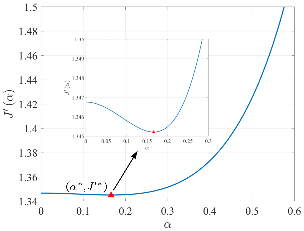
Figure 3: Loss function $J^{\prime}\left(\alpha\right)$ when choosing different chattering attenuation rate $\alpha$ in problem (45a).

Theorem 3 provides a fully analytical optimal solution for problem (45a). The optimal solution of problem (45a) is shown in Fig. 4. In Fig. 4(a-b), the state vector ${\boldsymbol{y}}^{*}$, the costate vector ${\boldsymbol{p}}^{*}$, and the control $v^{*}$ chatter with a limit time point $\tau_{\infty}^{*}\approx 5.094$. $\widehat{{\mathcal{H}}}\equiv 0$ and the Bang-Singular-Bang control law can be observed. To further examine the behavior of the system approaching $\tau_{\infty}^{*}$, the time axes in Fig. 4(c-d) are in logarithmic scales, while the amplitudes of ${\boldsymbol{y}}$ and ${\boldsymbol{p}}$ are multiplied by some certain compensation factors. Then, both the state vector and the costate vector exhibit strict periodicity in Fig. 4(c-d), which can be reasoned by Proposition 14-2 and (68), respectively.

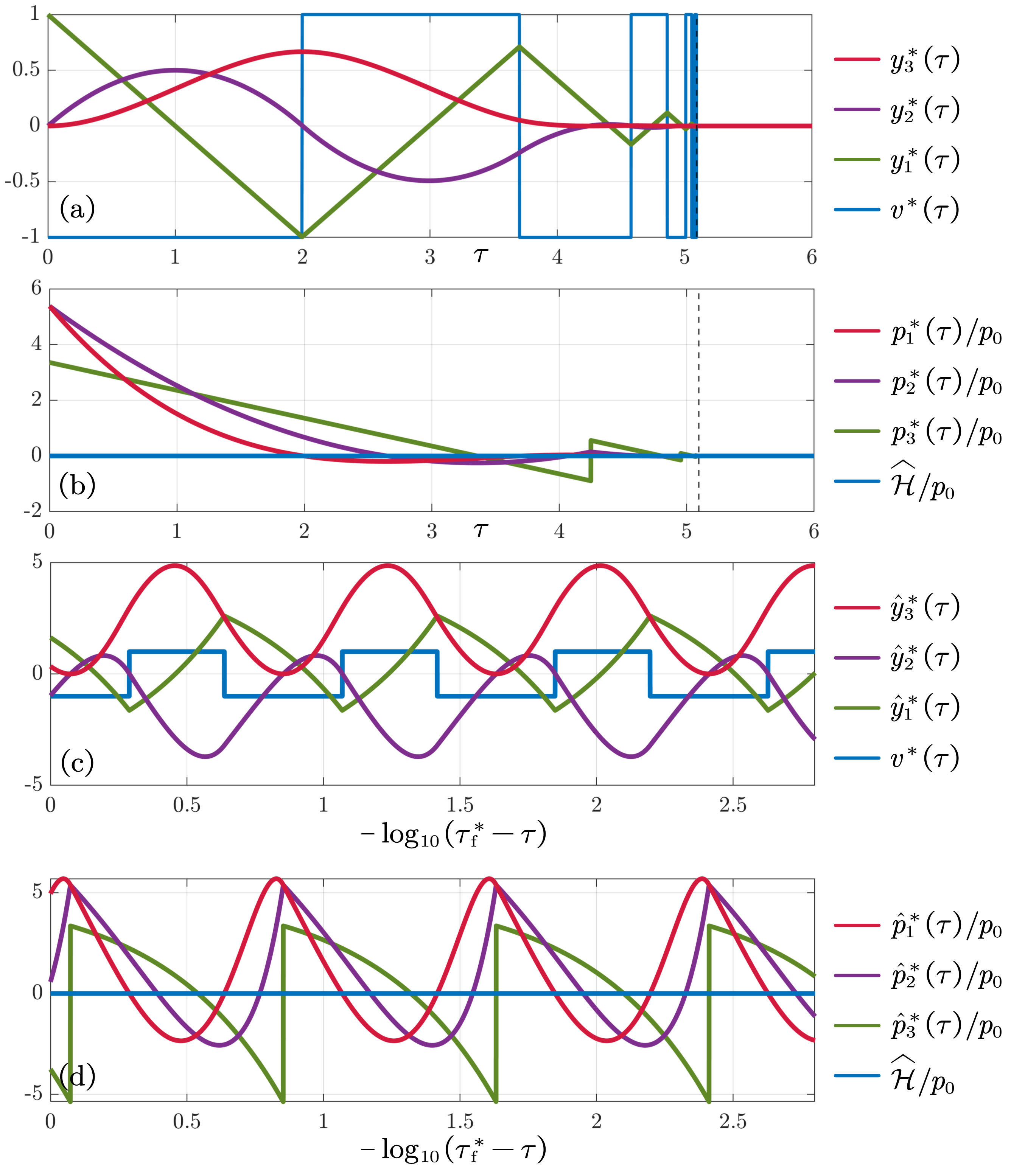
Figure 4: Optimal solution of problem (45a). (a) The optimal trajectory ${\boldsymbol{y}}^{*}\left(\tau\right)$ and the optimal control $v^{*}\left(\tau\right)$. (b) The optimal costate vector $\frac{1}{p_{0}}{\boldsymbol{p}}^{*}\left(\tau\right)$. (c-d) Enlargement of (a-b) during the chattering period. The abscissa is in logarithmic scale with respect to time, i.e., $-\log_{10}\left(\tau_{\infty}^{*}-\tau\right)$. $\forall k=1,2,3$, $\hat{y}_{k}^{*}\left(\tau\right)=y_{k}^{*}\left(\tau\right)\left(1-\frac{\tau}{\tau_{\infty}^{*}}\right)^{-k}$, and $\hat{p}_{k}^{*}\left(\tau\right)=p_{k}^{*}\left(\tau\right)\left(1-\frac{\tau}{\tau_{\infty}^{*}}\right)^{k-4}$.

V-D Optimal Solution for Problem (43a)

Section V-A provides the equivalence between problem (43a) and problem (45a) in Theorem 2, while Section V-B and Section V-C successfully solve problem (45a) strictly in Theorem 3. Therefore, the optimal solution for problem (43a) can be directly obtained by Theorem 2.

Theorem 4.

Apply the values in (65), (66), and (76). Assume that in problem (43a), $x_{{\mathrm{f}}4}-x_{0,4}\geq-\frac{x_{0,1}}{M_{0}}\left(\frac{x_{0,1}^{3}}{M_{0}^{2}}J^{\prime*}+M_{3}\tau_{\infty}^{*}\right)$. Then, a chattering phenomenon occurs in the optimal solution of problem (43a).

1. $\forall i\in{\mathbb{N}}$, $t_{i}=-\frac{x_{0,1}}{M_{0}}\tau_{i}^{*}=-\frac{x_{0,1}\left(1-{\alpha^{*}}^{i}\right)}{M_{0}\left(1-\alpha^{*}\right)}\tau_{1}^{*}$ is the junction time of $\lambda_{3}$. Then, $x_{1}^{*}\left(t_{i}\right)={\alpha^{*}}^{i}x_{0,1}$, $x_{2}^{*}\left(t_{i}\right)=0$, $x_{3}^{*}\left(t_{i}\right)=M_{3}$, and $x_{4}^{*}\left(t_{i}\right)=x_{\infty,4}-{\alpha^{*}}^{4i}\left(x_{\infty,4}-x_{0,4}\right)$. Among them, $t_{\infty}^{*}=-\frac{x_{0,1}}{M_{0}}\tau_{\infty}^{*}$ is the chattering limit time, and $x_{\infty,4}=x_{4}^{*}\left(t_{\infty}^{*}\right)=x_{0,4}-\frac{x_{0,1}}{M_{0}}\left(\frac{x_{0,1}^{3}}{M_{0}^{2}}J^{\prime*}+M_{3}\tau_{\infty}^{*}\right)$. Specifically, ${\boldsymbol{x}}^{*}\left(t_{\infty}^{*}\right)=\left(0,0,M_{3},x_{\infty,4}\right)$.

2. $\forall i\in{\mathbb{N}}$, the optimal control in $\left(t_{i-1},t_{i}\right)$ is $\forall\beta\in\left(0,1\right)$,

   $$u^{*}\left(\left(1-\beta\right)t_{i-1}+\beta t_{i}\right)=\begin{dcases}M_{0},&\beta\in\left(0,\beta_{1}\right),\\ -M_{0},&\beta\in\left(\beta_{1},\beta_{2}\right),\\ M_{0},&\beta\in\left(\beta_{2},1\right).\end{dcases}$$ (77)

   $\forall t\in\left(t_{\infty}^{*},t_{\mathrm{f}}^{*}\right)$, $x_{3}^{*}\left(t\right)\equiv M_{3}$, $u^{*}\left(t\right)\equiv 0$, where $t_{\mathrm{f}}^{*}=t_{\infty}^{*}+\frac{x_{{\mathrm{f}}4}-x_{\infty,4}}{M_{3}}$.

Proof.

Theorem 4 holds due to Theorems 2 and 3. ∎

Theorem 5.

In time-optimal control problem (1a) for chain-of-integrators system with state constraints, denote the order as $n$ and denote the state constraint inducing chattering as $s$.

1. Chattering phenomena do not occur when $n\leq 3$ or when $n=4$ and $\left|s\right|\not=3$.

2. The case where $n=4$ and $\left|s\right|=3$ represents problems of the lowest order that allow chattering. Theorem 4 provides a set of examples for chattering optimal control.

3. Chattering phenomena can occur when $n\geq 5$.

Proof.

Analysis in Section IV and Section V prove Theorem 5-1 and Theorem 5-2, respectively. For $n\geq 5$, let $s=\overline{3}$ as the unique state constraint. $x_{0,1:4}$ and $x_{{\mathrm{f}},1:4}$ are the same to problem (43a), while $x_{0,5:n}$ is given arbitrarily. Let $u^{*}$ be the optimal control of problem (43a). Construct the terminal state vector ${\boldsymbol{x}}_{\mathrm{f}}$ by ${\boldsymbol{x}}_{0}$ and $u^{*}$ directly. Then, $u^{*}$ is also the optimal control of the above problem where $n\geq 5$. Note that $u^{*}$ chatters. Therefore, Theorem 5-3 holds. ∎

Two feasible solutions for problem (43a) should be compared. The first one is the optimal trajectory given in 4, where

$$t_{\infty}^{*}\approx 5.0938\frac{\left|x_{0,1}\right|}{M_{0}},\,t_{\mathrm{f}}^{*}\approx\frac{x_{{\mathrm{f}}4}-x_{0,4}}{M_{3}}+1.3452\frac{x_{0,1}^{4}}{M_{0}^{3}M_{3}}.$$ (78)

The second one is the MIM-trajectory [14]. Let ${\boldsymbol{x}}$ moves from ${\boldsymbol{x}}_{0}$ to $x_{3}\equiv M_{3}$ as fast as possible. It can be calculated that

$$\hat{t}_{\infty}\approx 4.3903\frac{\left|x_{0,1}\right|}{M_{0}},\,\hat{t}_{\mathrm{f}}\approx\frac{x_{{\mathrm{f}}4}-x_{0,4}}{M_{3}}+1.3468\frac{x_{0,1}^{4}}{M_{0}^{3}M_{3}},$$ (79)

where ${\boldsymbol{x}}_{1:3}$ reaches $M_{3}{\boldsymbol{e}}_{3}$ at $\hat{t}_{\infty}$, and ${\boldsymbol{x}}$ reaches ${\boldsymbol{x}}_{\mathrm{f}}$ at $\hat{t}_{\mathrm{f}}$. The MIM-trajectory reaches the maximum speed stage for $t_{\infty}^{*}-\hat{t}_{\infty}\approx 0.1424\frac{\left|x_{0,1}\right|}{M_{0}}$ earlier than the optimal trajectory. However, the MIM-trajectory arrives at ${\boldsymbol{x}}_{\mathrm{f}}$ for $\hat{t}_{\mathrm{f}}-t_{\mathrm{f}}^{*}\approx\left(1.5425\times 10^{-3}\right)\frac{x_{0,1}^{4}}{M_{0}^{3}M_{3}}$ later than the optimal trajectory.

Moreover, the optimal trajectory and the MIM-trajectory of a 4th-order position-to-position problem with full state constraints are shown in Fig. 1(d) and (e), respectively. Among them, the optimal trajectory is obtained through careful derivation and costate analysis. The optimal terminal time is $t_{\mathrm{f}}^{*}\approx 12.6645$, while MIM’s terminal time is $\hat{t}_{\mathrm{f}}\approx 12.6667$, achieving a relative error of $0.17\%$. It is noteworthy that position-to-position snap-limited trajectories are universally applied as a reference in ultra-precision wafer stages. The chattering optimal trajectory can be applied in practice, since the trajectory is sampled by the finite control frequency.

VI Conclusion

This paper has set out to investigate chattering phenomena in a classical and open problem (1a), i.e., time-optimal control for high-order chain-of-integrators systems with full state constraints. However, there have existed neither proofs on non-existence nor counterexamples to the chattering phenomenon in the classical problem (1a) so far. This paper established a theoretical framework for the chattering phenomenon in problem (1a), pointing out that there exists at most one active state constraint during a chattering period. An upper bound on control’s switching times in an unconstrained arc during chattering is determined, and the convergence of states and costates at the chattering limit point is analyzed. This paper proved the existence of the chattering phenomenon in 4th order problems with velocity constraints in the presence of sufficient separation between the initial and terminal positions, where the decay rate in the time domain was precisely calculated as $\alpha^{*}\approx 0.1660687$. The conclusion can be applied to construct 4th order trajectories with full state constraints in strict time-optimality. To the best of our knowledge, the first strictly time-optimal 4th trajectory with full state constraints is provided in this paper, noting that position-to-position snap-limited trajectories with full state constraints are universally applied in ultra-precision control in the industry. Furthermore, this paper proves that chattering phenomena do not exist in other cases of other $n\leq 4$. In other words, 4th order problems with velocity constraints represent problems allowing chattering of the lowest order. The above conclusions correct the longstanding misconception in the industry regarding the time-optimality of S-shaped trajectories with minimal switching times.

Yunan Wang (S’22) received the B.S. degree in mechanical engineering, in 2022, from the Department of Mechanical Engineering, Tsinghua University, Beijing, China. He is currently working toward the Ph.D. degree in mechanical engineering. His research interests include optimal control, trajectory planning, toolpath planning, and precision motion control. He was the recipient of the Best Conference Paper Finalist at the 2022 International Conference on Advanced Robotics and Mechatronics, and 2021 Top Grade Scholarship for Undergraduate Students of Tsinghua University.

Chuxiong Hu (S’09-M’11-SM’17) received his B.S. and Ph.D. degrees in Mechatronic Control Engineering from Zhejiang University, Hangzhou, China, in 2005 and 2010, respectively. He is currently an Associate Professor (tenured) at Department of Mechanical Engineering, Tsinghua University, Beijing, China. From 2007 to 2008, he was a Visiting Scholar in mechanical engineering with Purdue University, West Lafayette, USA. In 2018, he was a Visiting Scholar in mechanical engineering with University of California, Berkeley, CA, USA. His research interests include precision motion control, high-performance multiaxis contouring control, precision mechatronic systems, intelligent learning, adaptive robust control, neural networks, iterative learning control, and robot. Prof. Hu was the recipient of the Best Student Paper Finalist at the 2011 American Control Conference, the 2012 Best Mechatronics Paper Award from the ASME Dynamic Systems and Control Division, the 2013 National 100 Excellent Doctoral Dissertations Nomination Award of China, the 2016 Best Paper in Automation Award, the 2018 Best Paper in AI Award from the IEEE International Conference on Information and Automation, and 2022 Best Paper in Theory from the IEEE/ASME International Conference on Mechatronic, Embedded Systems and Applications. He is now an Associate Editor for the IEEE Transactions on Industrial Informatics and a Technical Editor for the IEEE/ASME Transactions on Mechatronics.

Zeyang Li received the B.S. degree in mechanical engineering in 2021, from the School of Mechanical Engineering, Shanghai Jiao Tong University, Shanghai, China. He is currently working toward the M.S. degree in mechanical engineering with the Department of Mechanical Engineering, Tsinghua University, Beijing, China. His current research interests include the areas of optimal control and reinforcement learning.

Yujie Lin received the B.S. degree in mathematics and applied mathematics, in 2023, from the Department of Mathematical Sciences, Tsinghua University, Beijing, China. He is currently working toward the Ph.D. degree in mathematics, at Qiuzhen College, Tsinghua University. His research interests include 3&4-dimensional topology and knot theory.

Shize Lin received the B.S. degree in mechanical engineering, in 2020, from the Department of Mechanical Engineering, Tsinghua University, Beijing, China, where he is currently working toward the Ph.D. degree in mechanical engineering. His research interests include robotics, motion planning and precision motion control.

Suqin He received the B.S. degree in mechanical engineering from Department of Mechanical Engineering, Tsinghua University, Beijing, China, in 2016, and the Ph.D. degree in mechanical engineering from the Department of Mechanical Engineering, Tsinghua University, Beijing, China, in 2023. His research interests include multi-axis trajectory planning and precision motion control on robotics and CNC machine tools. He was the recipient of the Best Automation Paper from IEEE Internal Conference on Information and Automation in 2016.

References

- [1] W. Wang, C. Hu, K. Zhou, S. He, and L. Zhu, “Local asymmetrical corner trajectory smoothing with bidirectional planning and adjusting algorithm for cnc machining,” Robotics and Computer-Integrated Manufacturing, vol. 68, p. 102058, 2021.
- [2] Y. Wang, J. Wang, Y. Li, C. Hu, and Y. Zhu, “Learning latent object-centric representations for visual-based robot manipulation,” in 2022 International Conference on Advanced Robotics and Mechatronics (ICARM). IEEE, 2022, pp. 138–143.
- [3] G. Zhao and M. Zhu, “Pareto optimal multirobot motion planning,” IEEE Transactions on Automatic Control, vol. 66, no. 9, pp. 3984–3999, 2020.
- [4] J. Wang, C. Hu, Y. Wang, and Y. Zhu, “Dynamics learning with object-centric interaction networks for robot manipulation,” IEEE Access, vol. 9, pp. 68 277–68 288, 2021.
- [5] M. Li, Y. Zhu, K. Yang, L. Yang, C. Hu, and H. Mu, “Convergence rate oriented iterative feedback tuning with application to an ultraprecision wafer stage,” IEEE Transactions on Industrial Electronics, vol. 66, no. 3, pp. 1993–2003, 2018.
- [6] S. Güler, B. Fidan, S. Dasgupta, B. D. Anderson, and I. Shames, “Adaptive source localization based station keeping of autonomous vehicles,” IEEE Transactions on Automatic Control, vol. 62, no. 7, pp. 3122–3135, 2016.
- [7] M. I. Zelikin and V. F. Borisov, Theory of chattering control: with applications to astronautics, robotics, economics, and engineering. Springer Science & Business Media, 2012.
- [8] R. F. Hartl, S. P. Sethi, and R. G. Vickson, “A survey of the maximum principles for optimal control problems with state constraints,” SIAM review, vol. 37, no. 2, pp. 181–218, 1995.
- [9] G. Bartolini, S. Pillosu, A. Pisano, E. Usai et al., “Time-optimal stabilization for a third-order integrator: A robust state-feedback implementation,” Lecture notes in control and information sciences, pp. 131–144, 2002.
- [10] Z. Ma and S. Zou, Optimal Control Theory: The Variational Method. Springer, 2021.
- [11] R. Haschke, E. Weitnauer, and H. Ritter, “On-line planning of time-optimal, jerk-limited trajectories,” in 2008 IEEE/RSJ International Conference on Intelligent Robots and Systems. IEEE, 2008, pp. 3248–3253.
- [12] T. Kröger, “Opening the door to new sensor-based robot applications–the reflexxes motion libraries,” in 2011 IEEE International Conference on Robotics and Automation. IEEE, 2011, pp. 1–4.
- [13] L. Berscheid and T. Kröger, “Jerk-limited real-time trajectory generation with arbitrary target states,” in Robotics: Science and Systems, 2021.
- [14] Y. Wang, C. Hu, Z. Li, S. Lin, S. He, and Y. Zhu, “Time-optimal control for high-order chain-of-integrators systems with full state constraints and arbitrary terminal states (extended version),” arXiv preprint arXiv:2311.07039, 2024.
- [15] M. Li, Y. Zhu, K. Yang, and C. Hu, “A data-driven variable-gain control strategy for an ultra-precision wafer stage with accelerated iterative parameter tuning,” IEEE Transactions on Industrial Informatics, vol. 11, no. 5, pp. 1179–1189, 2015.
- [16] C. Marchal, “Chattering arcs and chattering controls,” Journal of Optimization Theory and Applications, vol. 11, pp. 441–468, 1973.
- [17] A. Fuller, “Study of an optimum non-linear control system,” International Journal of Electronics, vol. 15, no. 1, pp. 63–71, 1963.
- [18] H. Robbins, “Junction phenomena for optimal control with state-variable inequality constraints of third order,” Journal of Optimization Theory and Applications, vol. 31, pp. 85–99, 1980.
- [19] M. Heymann, F. Lin, G. Meyer, and S. Resmerita, “Analysis of zeno behaviors in a class of hybrid systems,” IEEE Transactions on Automatic Control, vol. 50, no. 3, pp. 376–383, 2005.
- [20] A. Lamperski and A. D. Ames, “Lyapunov theory for zeno stability,” IEEE Transactions on Automatic Control, vol. 58, no. 1, pp. 100–112, 2012.
- [21] I. Kupka, “Fuller’s phenomena,” in Perspectives in Control Theory: Proc. Conf. Sielpia, 1988, pp. 129–142.
- [22] M. Borshchevskii and I. Ioslovich, “The problem of the optimum rapid braking of an axisymmetric solid rotating around its centre of mass,” Journal of Applied Mathematics and Mechanics, vol. 49, no. 1, pp. 30–41, 1985.
- [23] J. Zhu, E. Trélat, and M. Cerf, “Minimum time control of the rocket attitude reorientation associated with orbit dynamics,” SIAM Journal on Control and Optimization, vol. 54, no. 1, pp. 391–422, 2016.
- [24] S. He, C. Hu, Y. Zhu, and M. Tomizuka, “Time optimal control of triple integrator with input saturation and full state constraints,” Automatica, vol. 122, p. 109240, 2020.
- [25] B. Ezair, T. Tassa, and Z. Shiller, “Planning high order trajectories with general initial and final conditions and asymmetric bounds,” The International Journal of Robotics Research, vol. 33, no. 6, pp. 898–916, 2014.
- [26] A. A. Agrachev and Y. Sachkov, Control theory from the geometric viewpoint. Springer Science & Business Media, 2013, vol. 87.
- [27] H. Schättler and U. Ledzewicz, Geometric optimal control: theory, methods and examples. Springer, 2012, vol. 38.
- [28] M. Zelikin and V. Borisov, “Optimal chattering feedback control,” Journal of Mathematical Sciences, vol. 114, no. 3, pp. 1227–1344, 2003.
- [29] J. Laurent-Varin, J. F. Bonnans, N. Bérend, M. Haddou, and C. Talbot, “Interior-point approach to trajectory optimization,” Journal of Guidance, Control, and Dynamics, vol. 30, no. 5, pp. 1228–1238, 2007.
- [30] M. Caponigro, R. Ghezzi, B. Piccoli, and E. Trélat, “Regularization of chattering phenomena via bounded variation controls,” IEEE Transactions on Automatic Control, vol. 63, no. 7, pp. 2046–2060, 2018.
- [31] C. Fox, An introduction to the calculus of variations. Courier Corporation, 1987.
- [32] E. M. Stein and R. Shakarchi, Real analysis: measure theory, integration, and Hilbert spaces. Princeton University Press, 2009.
- [33] R. Bellman, “On the theory of dynamic programming,” Proceedings of the national Academy of Sciences, vol. 38, no. 8, pp. 716–719, 1952.
- [34] D. H. Jacobson, M. M. Lele, and J. L. Speyer, “New necessary conditions of optimality for control problems with state-variable inequality constraints,” Journal of mathematical analysis and applications, vol. 35, no. 2, pp. 255–284, 1971.