How Private is DP-SGD?
Abstract
We demonstrate a substantial gap between the privacy guarantees of the Adaptive Batch Linear Queries (ABLQ) mechanism under different types of batch sampling: (i) Shuffling, and (ii) Poisson subsampling; the typical analysis of Differentially Private Stochastic Gradient Descent (DP-SGD) follows by interpreting it as a post-processing of ABLQ. While shuffling based DP-SGD is more commonly used in practical implementations, it is neither analytically nor numerically amenable to easy privacy analysis. On the other hand, Poisson subsampling based DP-SGD is challenging to scalably implement, but has a well-understood privacy analysis, with multiple open-source numerically tight privacy accountants available. This has led to a common practice of using shuffling based DP-SGD in practice, but using the privacy analysis for the corresponding Poisson subsampling version. Our result shows that there can be a substantial gap between the privacy analysis when using the two types of batch sampling, and thus advises caution in reporting privacy parameters for DP-SGD.
1 Introduction
Using noisy gradients in first order methods such as stochastic gradient descent has become a prominent approach for adding differential privacy () to the training of differentiable models such as neural networks. This approach, introduced by Abadi et al. (2016), has come to be known as Differentially Private Stochastic Gradient Descent, and we use the term DP-SGD to refer to any such first order method. DP-SGD is currently the canonical algorithm for training deep neural networks with privacy guarantees, and there currently exist multiple open source implementations, such as in Tensorflow Privacy (a), Pytorch Opacus (Yousefpour et al., 2021), and JAX Privacy (Balle et al., 2022). The algorithm has been applied widely in various machine learning domains, such as training of image classification (Tramer & Boneh, 2020; Papernot et al., 2021; Klause et al., 2022; De et al., 2022; Bu et al., 2022), generative models with GAN (Torkzadehmahani et al., 2019; Chen et al., 2020), diffusion models (Dockhorn et al., 2022), language models (Li et al., 2021; Yu et al., 2021; Anil et al., 2022; He et al., 2022), medical imaging (Ziller et al., 2021), as well as private spatial querying (Zeighami et al., 2021), ad modeling (Denison et al., 2023), and recommendation (Fang et al., 2022).
DP-SGD operates by processing the training data in mini-batches, and at each step, performs a first order gradient update, using a noisy estimate of the average gradient for each mini-batch. In particular, the gradient for each record is first clipped to have a pre-determined bounded -norm, by setting , and then adding Gaussian noise of standard deviation to all coordinates of the sum of gradients in the mini-batch.111While some distributed training setup uses the sum gradient directly, it is common to rescale the sum gradient by the batch size to obtain the average gradient before applying the optimization step. Since this scaling factor can be assimilated in the learning rate, we focus on the sum gradient for simplicity in this paper. The privacy guaranteed by the mechanism depends on the following: the choice of , the size of dataset, the number of steps of gradient update performed, and finally the process used to generate the batches. Almost all deep learning systems generate fixed-sized batches of data by going over the dataset sequentially. When feasible, a global shuffling of all the examples in the dataset is performed for each training epoch by making a single pass over the dataset. On the other hand, the process analyzed in Abadi et al. (2016) constructs each batch by including each record with a certain probability, chosen i.i.d. However, this leads to variable-sized mini-batches, which is technically challenging to handle in practice. As a result, there is generally a mismatch between the actual training pipeline and the privacy accounting in many applications of DP-SGD, with the implicit assumption that this subtle difference is negligible and excusable. However, in this paper, we show that this is not true—in a typical setting, as shown in Figure 1, the privacy loss from the correct accounting is significantly larger than expected.
Adaptive Batch Linear Queries and Batch Samplers.
Formally, the privacy analysis of DP-SGD, especially in the case of non-convex differentiable models, is performed by viewing it as a post-processing of a mechanism performing adaptive batch linear queries () as defined in Algorithm 1 (we use subscript to emphasize the role of the batch sampler), where the linear query corresponds to the clipped gradient corresponding to record . For any , we require that . Note that without loss of generality, we can treat the norm bound by defining for the corresponding gradient , and rescaling by to get back the noisy gradient for DP-SGD.
As mentioned above, a canonical way to generate the mini-batches is to go through the dataset in a fixed deterministic order, and divide the data into mini-batches of a fixed size (Algorithm 2, denoted as ). Another commonly used option is to first randomly permute the entire dataset before dividing it into mini-batches of a fixed size (Algorithm 3, denoted as ); this option provides amplification by shuffling, namely, that the privacy guarantees are better compared to fixed deterministic ordering. However, obtaining such amplification bounds is non-trivial, and while some bounds have been recently established for such privacy amplification (Erlingsson et al., 2019; Feldman et al., 2021, 2023), they tend to be loose and only kick in when the basic mechanism is already sufficiently private.
Instead, the approach followed by Abadi et al. (2016), and henceforth used commonly in reporting privacy parameters for DP-SGD, is to assume that each batch is sampled i.i.d. by including each record with a certain probability, referred to as Poisson subsampling (Algorithm 4, denoted as ). The advantage of this approach is that the privacy analysis of such sampling is easy to carry out since the mechanism can be viewed as a composition of independent sub-mechanisms. This enables privacy accounting methods such as Rényi DP (Mironov, 2017) as well as numerically tight accounting methods using privacy loss distributions (elaborated on later in Section 3).
This has been the case, even when the algorithm being implemented in fact uses some form of shuffling based batch sampler. To quote Abadi et al. (2016) (with our emphasis),
“In practice, for efficiency, the construction of batches and lots is done by randomly permuting the examples and then partitioning them into groups of the appropriate sizes. For ease of analysis, however, we assume that each lot is formed by independently picking each example with probability , where is the size of the input dataset.”
Most implementations of DP-SGD mentioned earlier also use some form of shuffling, with a rare exception of PyTorch Opacus (Yousefpour et al., 2021) that has the option of Poisson subsampling to be consistent with the privacy analysis. But this approach does not scale to large datasets as random access for datasets that do not fit in memory is generally inefficient. Moreover, variable batch sizes are inconvenient to handle in deep learning systems222For example, when the input shape changes, jax.jit will trigger recompilation, and tf.function will retrace the graph. Google TPUs require all operations to have fixed (input and output) shapes. Moreover, in various form of data parallelism, the batch size needs to be divisible by the number of accelerators.. Tensorflow Privacy (b) provides the compute_dp_sgd_privacy_statement method for computing the privacy parameters and reminds users about the implicit assumption of Poisson subsampling. Ponomareva et al. (2023) note in their survey that “It is common, though inaccurate, to train without Poisson subsampling, but to report the stronger DP bounds as if amplification was used.”
As DP-SGD is being deployed in more applications with such discrepancy, it has become crucial to understand exactly how the privacy guarantee depends on the precise choice of the batch sampler, especially when one cares about specific privacy parameters (and not asymptotic bounds). This leads us to the main question motivating this work:
How do the privacy guarantees of compare when using different batch samplers ?
1.1 Our Contributions
We study the privacy guarantees of for different choices of batch samplers . While we defer the formal definition of - to Section 2, let denote the privacy loss curve of for any , for a fixed choice of and . Namely, for all , let be the smallest such that satisfies - for any underlying adaptive query method . Let be defined analogously.
- vs .
-
We observe that always satisfies stronger privacy guarantees than , i.e., for all .
- vs .
-
We show that the privacy guarantee of and are incomparable. Namely, for all values of (number of steps) and (noise parameter), it holds (i) for small enough that , but perhaps more surprisingly, (ii) for sufficiently large it holds that . We also demonstrate this separation in a specific numerical setting of parameters.
- vs .
-
By combining the above it follows that for sufficiently large , it holds that . If were to hold for all , then reporting privacy parameters for would provide correct, even if pessimistic, privacy guarantees for . However, we demonstrate multiple concrete settings of parameters, for which , or alternately, .
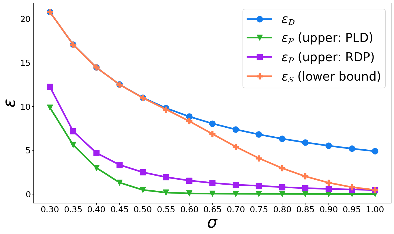
For example, in Figure 1, we fix and the number of steps , and compare the value of for various values of . In particular, for , we find that which could be considered as a reasonable privacy guarantee, but .
This suggests that reporting privacy guarantees using the Poisson batch sampler can significantly underestimate the privacy loss when in fact the implementation uses the shuffle batch sampler.
Our main takeaway is that batch sampling plays a crucial in determining the privacy guarantees of , and hence caution must be exercised in reporting privacy parameters for mechanisms such as DP-SGD.
1.2 Technical Overview
Our techniques relies on the notion of dominating pairs as defined by Zhu et al. (2022) (see Definition 2.3), which if tightly dominating captures the privacy loss curve .
- vs .
-
We observe that applying a mechanism on a random permutation of the input dataset does not degrade its privacy guarantees. While standard, we include a proof for completeness.
- vs .
-
In order to show that for small enough , we first show that by showing that the total variation distance between the tightly dominating pair for is larger than that in the case of . And thus, by the continuity of hockey stick divergence in , we obtain the same for small enough .
In order to show that for large enough , we demonstrate an explicit set (a halfspace), which realizes a lower bound on the hockey stick divergence between the tightly dominating pair of , and show that this decays slower than the hockey stick divergence between the tightly dominating pair for .
We demonstrate the separation in a specific numerical settings of parameters by using the dp_accounting library (Google’s DP Library., 2020) to provide lower bounds on the hockey stick divergence between the tightly dominating pair for .
- vs .
-
One challenge in understanding the privacy guarantee of is the lack of a clear dominating pair for the mechanism. Nevertheless, we consider a specific instance of the query method , and a specific adjacent pair . The key insight we use in constructing this and is that in the case of , since the batches are of a fixed size, the responses to queries on batches containing only the non-differing records in and can leak information about the location of the differing record in the shuffled order. This limitation is not faced by , since each record is independently sampled in each batch. We show a lower bound on the hockey stick divergence between the output distribution of the mechanism on these adjacent inputs, by constructing an explicit set , thereby obtaining a lower bound on .
In order to show that this can be significantly larger than the privacy guarantee of , we again use the dp_accounting library, this time to provide upper bounds on the hockey stick divergence between the dominating pair of .
We provide the IPython notebook (Google Colab link) that was used for all the numerical demonstrations; the entire notebook executes in a few minutes when using a free CPU runtime on Google Colab .
2 Differential Privacy
We consider mechanisms that map input datasets to distributions over an output space, namely . That is, on input dataset where each record , is a probability distribution over the output space . Two datasets and are said to be adjacent, denoted , if, loosely speaking, they “differ in one record”. This can be formalized in multiple ways, which we elaborate on in Section 2.2, but for any notion of adjacency, Differential Privacy (DP) can be defined as follows.
Definition 2.1 (DP).
For , a mechanism satisfies - if for all “adjacent” datasets , and for any (measurable) event it holds that
For any mechanism , let be its privacy loss curve, namely is the smallest for which satisfies -; can be defined analogously.
2.1 Adaptive Batch Linear Queries Mechanism
We primarily study the adaptive batch linear queries mechanism using a batch sampler and an adaptive query method , as defined in Algorithm 1. The batch sampler can be instantiated with any algorithm that produces a (randomized) sequence of batches . produces a sequence of responses where each . The response is produced recursively using the adaptive query method that given , constructs a new query (for ), and we estimate the average value of over the batch with added zero-mean Gaussian noise of scale to all coordinates. As explained in Section 1, DP-SGD falls under this abstraction by considering an adaptive query method that is specified by a differentiable loss function , and starts with an initial , and defines the query as the clipped gradient where is the -th model iterate recursively obtained by performing gradient descent, e.g., (or any other first order optimization step).
We consider the Deterministic (Algorithm 2), Poisson (Algorithm 4) and Shuffle (Algorithm 3) batch samplers. As used in Section 1, we will continue to use as a shorthand for denoting the privacy loss curve of for any . Namely, for all , let be the smallest such that satisfies - for all choices of the underlying adaptive query method . And is defined analogously.
2.2 Adjacency Notions
As alluded to earlier, the notion of adjacency is crucial to Definition 2.1. Commonly used adjacency notions are:
- Add-Remove adjacency.
-
Datasets are said to be add-remove adjacent if there exists an such that or vice-versa (where represents the dataset obtained by removing the -th record in ).
- Substitution adjacency.
-
Datasets are said to be substitution adjacent if there exists an such that and .
The privacy analysis of DP-SGD is typically done for the Poisson batch sampler (Abadi et al., 2016; Mironov, 2017), with respect to the add-remove adjacency. However, it is impossible to analyze the privacy of or with respect to the add-remove adjacency because the batch samplers and require that the number of records equals . On the other hand, using the substitution adjacency for and leads to an unfair comparison to whose analysis is with respect to the add-remove adjacency. Thus, to make a fair comparison, we consider the following adjacency (considered by Kairouz et al. (2021)).
- Zero-out adjacency.
-
We augment the input space to be and extend any adaptive query method as for all . Datasets are said to be zero-out adjacent if there exists such that , and exactly one of is in and the other is . Whenever we need to specifically emphasize that and , we will denote it as . In this notation, if either or .
The privacy analysis of with respect to zero-out adjacency is the same as that with respect to the add-remove adjacency; it is essentially replacing a record by a “ghost” record that makes the query method always return . In the rest of this paper, we only consider this zero-out adjacency.
2.3 Hockey Stick Divergence
We interchangeably use the same notation (e.g., letters such as ) to denote both a probability distribution and its corresponding density function. For and positive semi-definite , we use to denote the Gaussian distribution with mean and covariance . For probability densities and , we use to denote the weighted sum of the corresponding densities. denotes the product distribution sampled as for , , and, denotes the -fold product distribution .
Definition 2.2.
For all , the -hockey stick divergence between and is .
It is immediate to see that satisfies - iff for all adjacent , it holds that .
Definition 2.3 (Dominating Pair (Zhu et al., 2022)).
The pair dominates the pair if holds for all . We say that dominates a mechanism if dominates for all adjacent .
If dominates , then for all , . We say that tightly dominates a mechanism if dominates and there exist adjacent datasets such that holds for all (note that this includes ); in this case, . Thus, tightly dominating pairs completely characterize the privacy loss of a mechanism (although they are not guaranteed to exist for all mechanisms.) Dominating pairs behave nicely under mechanism compositions. Namely, if dominates and dominates , then dominates the (adaptively) composed mechanism .
3 Dominating Pairs for
We discuss the dominating pairs for for that will be crucial for establishing our results.
Tightly dominating pair for .
It follows from the standard analysis of the Gaussian mechanism and parallel composition that a tightly dominating pair for is the pair , leading to a closed-form expression for .
Proposition 3.1 (Theorem 8 in Balle & Wang (2018)).
For all , it holds that
where is the cumulative density function (CDF) of the standard normal random variable .
Tightly dominating pair of .
Zhu et al. (2022) showed that the tightly dominating pair for a single step of , a Poisson sub-sampled Gaussian mechanism, is given by the pair , where is the sub-sampling probability of each record, namely , and in the case where , we have . Since is a -fold composition of this Poisson subsampled Gaussian mechanism, it follows that the tightly dominating pair for is .
The hockey stick divergence does not have a closed-form expression, but there are privacy accountants based on the methods of Rényi differential privacy (RDP) (Mironov, 2017) as well as privacy loss distributions (PLD) (Meiser & Mohammadi, 2018; Sommer et al., 2019), the latter providing numerically accurate algorithms (Koskela et al., 2020; Gopi et al., 2021; Ghazi et al., 2022; Doroshenko et al., 2022), and have been the basis of multiple open-source implementations from both industry and academia including Prediger & Koskela (2020); Google’s DP Library. (2020); Microsoft. (2021). While Rényi-DP based accounting provides an upper bound on , the PLD based accounting implementations can provide upper and lower bounds on to high accuracy, as controlled by a certain discretization parameter.
Tightly dominating pair for ?
It is not clear which adjacent pair would correspond to a tightly dominating pair for , and moreover, it is even a priori unclear if one even exists. However, in order to prove lower bounds on the privacy parameters, it suffices to consider a specific instantiation of the adaptive query method , and a particular adjacent pair . In particular, we instantiate the query method as follows.
Consider the input space , and assume that the query method is non-adaptive, and always produces the query . We consider the adjacent datasets:
-
•
, and
-
•
.
In this case, it is easy to see that the distributions and are given as:
where denotes the all-’s vector in and denotes the -th standard basis vector in . Shifting the distributions by does not change the hockey stick divergence , hence we might as well consider the pair
| (1) | ||||
| (2) |
Thus, . We conjecture that this pair is in fact tightly dominating for for all instantiations of query methods (including adaptive ones). We elaborate more in Section 4.3.1.
Conjecture 3.2.
The pair tightly dominates for all adaptive query methods .
The results in this paper do not rely on this conjecture being true, as we only use the dominating pair to establish lower bounds on .
4 Privacy Loss Comparisons
4.1 vs
We first note that enjoys stronger privacy guarantees than .
Theorem 4.1.
For all , it holds that .
This follows from a standard technique that shuffling cannot degrade the privacy guarantee satisfied by a mechanism. For completeness, we provide a proof in Appendix B.
4.2 vs
We show that and have incomparable privacy loss. In particular, we show the following.
Theorem 4.2.
There exist such that,
-
(a)
: it holds that , and
-
(b)
: it holds that .
We use the Gaussian measure of a halfspace.
Proposition 4.3.
For and the set ,
Proof of Theorem 4.2.
We prove each part as follows:
For part (a), first we consider the case of . In this case, is simply the total variation distance between and . Recall that and , where and . Observe that . Thus, we have that
Note that the inequality above is strict. Since is continuous in (see Proposition C.2), there exists some , such that for all , .
For part (b), we construct an explicit bad event such that . In particular, we consider:
The choice of is such that,
Hence it follows that , or equivalently, . This implies that .
Next, we obtain a lower bound on . For and , it holds that
| (3) |
where we use Proposition 4.3 in the last two steps. On the other hand, we have from Proposition 3.1 that
| (4) |
There exists a sufficiently large such that
| (5) | ||||
| (6) | ||||
by noting that for large the most significant term inside in Equation 5 is , whereas in Equation 6 the most significant term inside is , which decreases much faster as , for a fixed and . ∎
Even though Theorem 4.2 was proved for some values of and , we conjecture that it holds for .
Conjecture 4.4.
Theorem 4.2 holds for .
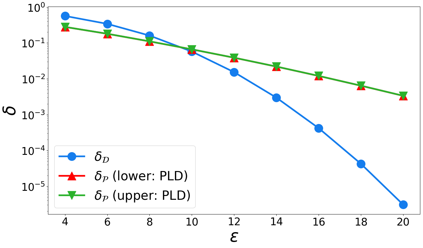
We do not rely on this conjecture being true in the rest of this paper. We provide a numerical example that validates Theorem 4.2 and provides evidence for 4.4. In Figure 2, for and , we plot the numerically computed (using Proposition 3.1), as well as lower and upper bounds on , computed using the open source dp_accounting library (Google’s DP Library., 2020).
4.3 vs
From Theorems 4.1 and 4.2, it follows that there exists an such that for all , it holds that . On the other hand, while we know that for sufficiently small , this does not imply anything about the relationship between and for small .
We demonstrate simple numerical settings where is significantly larger than . We prove lower bounds on by constructing specific sets and using the fact that .
In particular, we consider sets parameterized by of the form ; note that is the complement of -fold Cartesian product of the set . For a single Gaussian distribution , we can compute the probability mass of under measure as:
In particular, when is for any standard basis vector , we have . Thus, we have that is
Similarly, we have .
Thus, we use the following lower bound:
| (7) |
for any suitable set that can be enumerated over. In our experiments described below, we set to be the set of all values of ranging from to in increments of .
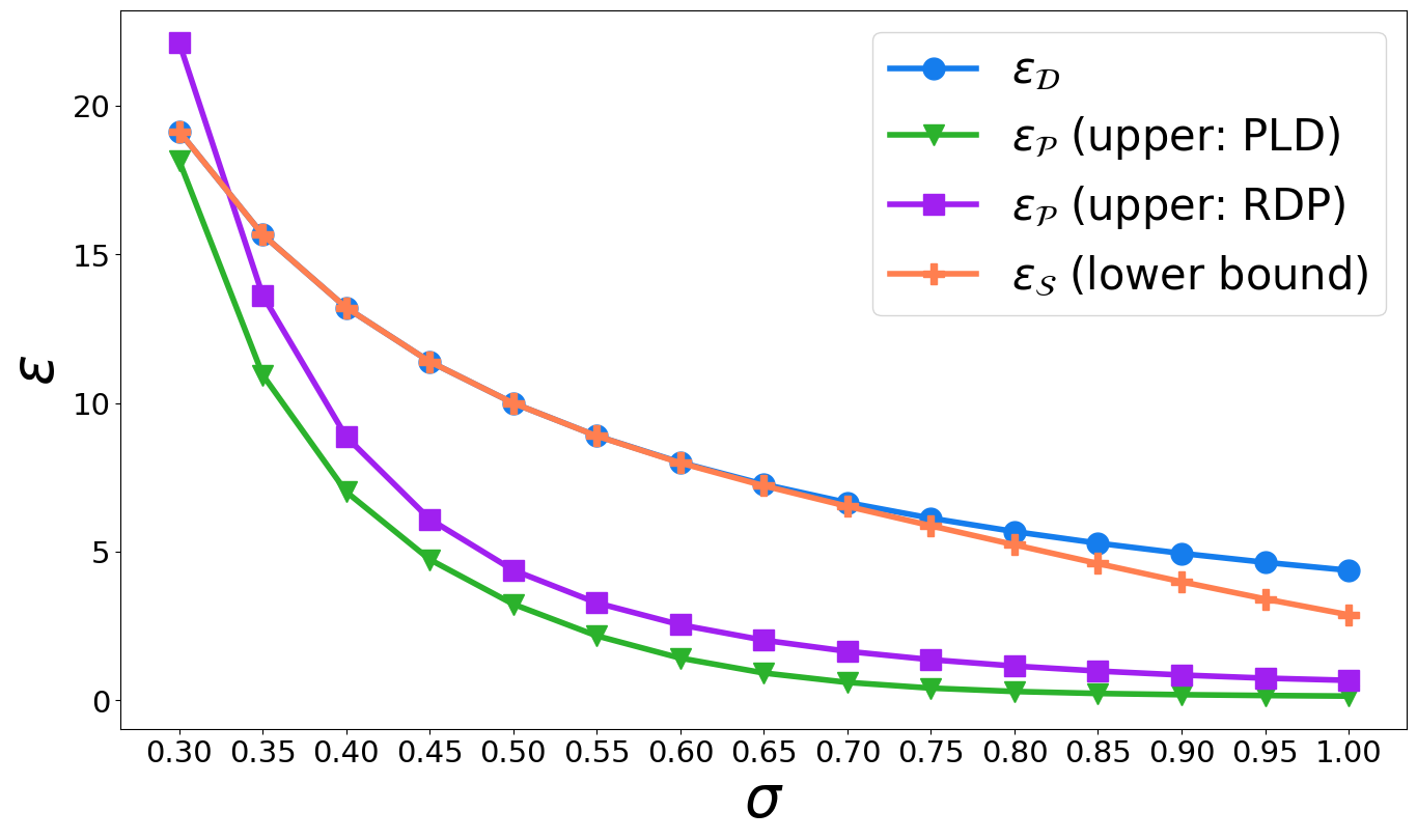
In Figure 3, we set and number of steps and plot , an upper bound on (obtained using dp_accounting) and a lower bound on as obtained via Equation 7. We find that while , , that is close to . Even is larger than . While the - guarantee of could have been considered as sufficiently private, only satisfies much worse privacy guarantees. We provide additional examples in Appendix A.
4.3.1 Intuition for 3.2
We attempt to shed some intuition for why does not provide as much amplification over , compared to , and why we suggest 3.2.
For sake of intuition, let’s consider the setting where the query method always generates the query , and we have two adjacent datasets:
-
•
, and
-
•
.
The case of is not valid, since in this case . However, we can still ask how well the privacy of the -th example is preserved by , by considering the hockey stick divergence between and .
The crucial difference between and is that the privacy analysis of does not depend at all on the non-differing records in the two datasets. In the case of , we observe that for any fixed and , the hockey stick divergence approaches as . We sketch this argument intuitively: For any batch that does not contain , the corresponding for . Whereas for the batch that contains , the corresponding in case of input or in case of input . As , we can identify the batch that contains with probability approaching , thereby not providing any amplification.
In summary, the main differing aspect about and is that in the former, the non-differing examples can leak information about the location of the differing example in the shuffled order, whereas that is not the case in the latter. While we sketched an argument that works asymptotically as , we see glimpses of it already at .
Our intuitive reasoning behind 3.2 is that even in the case of (vector valued) adaptive query methods, in order to “leak the most information” about the differing record between and , it seems natural that the query should evaluate to for all . If the query method satisfies this condition for all , then it is easy to show that tightly dominates . 3.2 then asserts that this is indeed the worst case.
5 Conclusion & Future Directions
We identified significant gaps between the privacy analysis of adaptive batch linear query mechanisms, under the deterministic, Poisson, and shuffle batch samplers. We find that while shuffling always provides better privacy guarantees over deterministic batching, Poisson batch sampling can provide a worse privacy guarantee than even deterministic sampling at large . But perhaps most surprisingly, we demonstrate that the amplification guarantees due to shuffle batch sampling can be severely limited compared to the amplification due to Poisson subsampling, in various regimes that could be considered of practical interest.
There are several interesting directions that remain to be investigated. In our work, we provide a technique to only provide a lower bound on the privacy guarantee when using a shuffle batch sampler. It would be interesting to have a tight accounting method for . A first step towards this could be to establish 3.2, which if true, might make numerical accountants for computing the hockey stick divergence possible. While this involves computing a high dimensional integral, it might be possible to approximate using importance sampling; e.g., such approaches have been attempted for (Wang et al., 2023).
However, it remains to be seen how the utility of DP-SGD would be affected when we use the correct privacy analysis for instead of the analysis for , which has been used extensively so far and treated as a good “approximation”. Alternative approaches such as (Kairouz et al., 2021; McMahan et al., 2022) that do not rely on amplification might turn out to be better if we instead use the correct analysis for , in the regimes where such methods are currently reported to under perform compared to DP-SGD.
Another important point to note is that the model of shuffle batch sampler we consider here is a simple one. There are various types of data loaders used in practice, which are not necessarily captured by our model. For example tf.data.Dataset.shuffle takes in a parameter of buffer size . It returns a random record among the first records, and immediately replaces it with the next record (-th in this case), and continues repeating this process. This leads to an asymmetric form of shuffling. Such batch samplers might thus require more careful privacy analysis.
The notion of DP aims to guarantee privacy even in the worst case. For example in the context of DP-SGD, it aims to protect privacy of a single record even when the model trainer and all other records participating in the training are colluding to leak information about this one record. And moreover, releasing the final model is assumed to leak as much information as releasing all intermediate iterates. Such strong adversarial setting might make obtaining good utility to be difficult. Alternative techniques for privacy amplification such as amplification by iteration (Feldman et al., 2018; Altschuler & Talwar, 2022) or through convergence of Langevin dynamics (Chourasia et al., 2021) have been studied, where only the last iterate of the model is released. However, these analyses rely on additional assumptions such as convexity and smoothness of the loss functions. Investigating whether it is possible to relax these assumptions to make amplification by iteration applicable to non-convex models is an interesting future direction.
References
- Abadi et al. (2016) Abadi, M., Chu, A., Goodfellow, I. J., McMahan, H. B., Mironov, I., Talwar, K., and Zhang, L. Deep learning with differential privacy. In Weippl, E. R., Katzenbeisser, S., Kruegel, C., Myers, A. C., and Halevi, S. (eds.), Proceedings of the 2016 ACM SIGSAC Conference on Computer and Communications Security, Vienna, Austria, October 24-28, 2016, pp. 308–318. ACM, 2016. doi: 10.1145/2976749.2978318. URL https://doi.org/10.1145/2976749.2978318.
- Altschuler & Talwar (2022) Altschuler, J. M. and Talwar, K. Privacy of noisy stochastic gradient descent: More iterations without more privacy loss. In Koyejo, S., Mohamed, S., Agarwal, A., Belgrave, D., Cho, K., and Oh, A. (eds.), Advances in Neural Information Processing Systems 35: Annual Conference on Neural Information Processing Systems 2022, NeurIPS 2022, New Orleans, LA, USA, November 28 - December 9, 2022, 2022. URL http://papers.nips.cc/paper_files/paper/2022/hash/18561617ca0b4ffa293166b3186e04b0-Abstract-Conference.html.
- Anil et al. (2022) Anil, R., Ghazi, B., Gupta, V., Kumar, R., and Manurangsi, P. Large-scale differentially private BERT. In Goldberg, Y., Kozareva, Z., and Zhang, Y. (eds.), Findings of the Association for Computational Linguistics: EMNLP 2022, Abu Dhabi, United Arab Emirates, December 7-11, 2022, pp. 6481–6491. Association for Computational Linguistics, 2022. doi: 10.18653/V1/2022.FINDINGS-EMNLP.484. URL https://doi.org/10.18653/v1/2022.findings-emnlp.484.
- Balle & Wang (2018) Balle, B. and Wang, Y. Improving the gaussian mechanism for differential privacy: Analytical calibration and optimal denoising. In Dy, J. G. and Krause, A. (eds.), Proceedings of the 35th International Conference on Machine Learning, ICML 2018, Stockholmsmässan, Stockholm, Sweden, July 10-15, 2018, volume 80 of Proceedings of Machine Learning Research, pp. 403–412. PMLR, 2018. URL http://proceedings.mlr.press/v80/balle18a.html.
- Balle et al. (2022) Balle, B., Berrada, L., De, S., Ghalebikesabi, S., Hayes, J., Pappu, A., Smith, S. L., and Stanforth, R. JAX-Privacy: Algorithms for privacy-preserving machine learning in jax, 2022. URL http://github.com/google-deepmind/jax_privacy.
- Bu et al. (2022) Bu, Z., Mao, J., and Xu, S. Scalable and efficient training of large convolutional neural networks with differential privacy. Advances in Neural Information Processing Systems, 35:38305–38318, 2022.
- Chen et al. (2020) Chen, D., Orekondy, T., and Fritz, M. Gs-wgan: A gradient-sanitized approach for learning differentially private generators. In Larochelle, H., Ranzato, M., Hadsell, R., Balcan, M., and Lin, H. (eds.), Advances in Neural Information Processing Systems, volume 33, pp. 12673–12684. Curran Associates, Inc., 2020. URL https://proceedings.neurips.cc/paper_files/paper/2020/file/9547ad6b651e2087bac67651aa92cd0d-Paper.pdf.
- Chourasia et al. (2021) Chourasia, R., Ye, J., and Shokri, R. Differential privacy dynamics of langevin diffusion and noisy gradient descent. In Ranzato, M., Beygelzimer, A., Dauphin, Y. N., Liang, P., and Vaughan, J. W. (eds.), Advances in Neural Information Processing Systems 34: Annual Conference on Neural Information Processing Systems 2021, NeurIPS 2021, December 6-14, 2021, virtual, pp. 14771–14781, 2021. URL https://proceedings.neurips.cc/paper/2021/hash/7c6c1a7bfde175bed616b39247ccace1-Abstract.html.
- De et al. (2022) De, S., Berrada, L., Hayes, J., Smith, S. L., and Balle, B. Unlocking high-accuracy differentially private image classification through scale. CoRR, abs/2204.13650, 2022. doi: 10.48550/ARXIV.2204.13650. URL https://doi.org/10.48550/arXiv.2204.13650.
- Denison et al. (2023) Denison, C., Ghazi, B., Kamath, P., Kumar, R., Manurangsi, P., Narra, K. G., Sinha, A., Varadarajan, A. V., and Zhang, C. Private ad modeling with DP-SGD. In Bagherjeiran, A., Djuric, N., Lee, K., Pang, L., Radosavljevic, V., and Rajan, S. (eds.), Proceedings of the Workshop on Data Mining for Online Advertising (AdKDD 2023) co-located with the 29th ACM SIGKDD Conference on Knowledge Discovery and Data Mining (KDD 2023), Long Beach, CA, USA, August 7, 2023, volume 3556 of CEUR Workshop Proceedings. CEUR-WS.org, 2023. URL https://ceur-ws.org/Vol-3556/adkdd23-denison-private-ceur-paper.pdf.
- Dockhorn et al. (2022) Dockhorn, T., Cao, T., Vahdat, A., and Kreis, K. Differentially private diffusion models. arXiv preprint arXiv:2210.09929, 2022.
- Doroshenko et al. (2022) Doroshenko, V., Ghazi, B., Kamath, P., Kumar, R., and Manurangsi, P. Connect the dots: Tighter discrete approximations of privacy loss distributions. Proc. Priv. Enhancing Technol., 2022(4):552–570, 2022. doi: 10.56553/POPETS-2022-0122. URL https://doi.org/10.56553/popets-2022-0122.
- Erlingsson et al. (2019) Erlingsson, Ú., Feldman, V., Mironov, I., Raghunathan, A., Talwar, K., and Thakurta, A. Amplification by shuffling: From local to central differential privacy via anonymity. In Chan, T. M. (ed.), Proceedings of the Thirtieth Annual ACM-SIAM Symposium on Discrete Algorithms, SODA 2019, San Diego, California, USA, January 6-9, 2019, pp. 2468–2479. SIAM, 2019. doi: 10.1137/1.9781611975482.151. URL https://doi.org/10.1137/1.9781611975482.151.
- Fang et al. (2022) Fang, L., Du, B., and Wu, C. Differentially private recommender system with variational autoencoders. Knowledge-Based Systems, 250:109044, 2022.
- Feldman et al. (2018) Feldman, V., Mironov, I., Talwar, K., and Thakurta, A. Privacy amplification by iteration. In Thorup, M. (ed.), 59th IEEE Annual Symposium on Foundations of Computer Science, FOCS 2018, Paris, France, October 7-9, 2018, pp. 521–532. IEEE Computer Society, 2018. doi: 10.1109/FOCS.2018.00056. URL https://doi.org/10.1109/FOCS.2018.00056.
- Feldman et al. (2021) Feldman, V., McMillan, A., and Talwar, K. Hiding among the clones: A simple and nearly optimal analysis of privacy amplification by shuffling. In 62nd IEEE Annual Symposium on Foundations of Computer Science, FOCS 2021, Denver, CO, USA, February 7-10, 2022, pp. 954–964. IEEE, 2021. doi: 10.1109/FOCS52979.2021.00096. URL https://doi.org/10.1109/FOCS52979.2021.00096.
- Feldman et al. (2023) Feldman, V., McMillan, A., and Talwar, K. Stronger privacy amplification by shuffling for renyi and approximate differential privacy. In Bansal, N. and Nagarajan, V. (eds.), Proceedings of the 2023 ACM-SIAM Symposium on Discrete Algorithms, SODA 2023, Florence, Italy, January 22-25, 2023, pp. 4966–4981. SIAM, 2023. doi: 10.1137/1.9781611977554.CH181. URL https://doi.org/10.1137/1.9781611977554.ch181.
- Ghazi et al. (2022) Ghazi, B., Kamath, P., Kumar, R., and Manurangsi, P. Faster privacy accounting via evolving discretization. In ICML, pp. 7470–7483, 2022.
- (19) Google Colab. URL https://colab.research.google.com/.
- Google’s DP Library. (2020) Google’s DP Library. DP Accounting Library. https://github.com/google/differential-privacy/tree/main/python/dp_accounting, 2020.
- Gopi et al. (2021) Gopi, S., Lee, Y. T., and Wutschitz, L. Numerical composition of differential privacy. In NeurIPS, pp. 11631–11642, 2021.
- He et al. (2022) He, J., Li, X., Yu, D., Zhang, H., Kulkarni, J., Lee, Y. T., Backurs, A., Yu, N., and Bian, J. Exploring the limits of differentially private deep learning with group-wise clipping. arXiv preprint arXiv:2212.01539, 2022.
- Kairouz et al. (2021) Kairouz, P., McMahan, B., Song, S., Thakkar, O., Thakurta, A., and Xu, Z. Practical and private (deep) learning without sampling or shuffling. In Meila, M. and Zhang, T. (eds.), Proceedings of the 38th International Conference on Machine Learning, ICML 2021, 18-24 July 2021, Virtual Event, volume 139 of Proceedings of Machine Learning Research, pp. 5213–5225. PMLR, 2021. URL http://proceedings.mlr.press/v139/kairouz21b.html.
- Klause et al. (2022) Klause, H., Ziller, A., Rueckert, D., Hammernik, K., and Kaissis, G. Differentially private training of residual networks with scale normalisation. arXiv preprint arXiv:2203.00324, 2022.
- Koskela et al. (2020) Koskela, A., Jälkö, J., and Honkela, A. Computing tight differential privacy guarantees using FFT. In AISTATS, pp. 2560–2569, 2020.
- Li et al. (2021) Li, X., Tramer, F., Liang, P., and Hashimoto, T. Large language models can be strong differentially private learners. arXiv preprint arXiv:2110.05679, 2021.
- McMahan et al. (2022) McMahan, B., Rush, K., and Thakurta, A. G. Private online prefix sums via optimal matrix factorizations. CoRR, abs/2202.08312, 2022. URL https://arxiv.org/abs/2202.08312.
- Meiser & Mohammadi (2018) Meiser, S. and Mohammadi, E. Tight on budget? Tight bounds for -fold approximate differential privacy. In CCS, pp. 247–264, 2018.
- Microsoft. (2021) Microsoft. A fast algorithm to optimally compose privacy guarantees of differentially private (DP) mechanisms to arbitrary accuracy. https://github.com/microsoft/prv_accountant, 2021.
- Mironov (2017) Mironov, I. Rényi differential privacy. In 30th IEEE Computer Security Foundations Symposium, CSF 2017, Santa Barbara, CA, USA, August 21-25, 2017, pp. 263–275. IEEE Computer Society, 2017. doi: 10.1109/CSF.2017.11. URL https://doi.org/10.1109/CSF.2017.11.
- Papernot et al. (2021) Papernot, N., Thakurta, A., Song, S., Chien, S., and Erlingsson, Ú. Tempered sigmoid activations for deep learning with differential privacy. In Proceedings of the AAAI Conference on Artificial Intelligence, volume 35, pp. 9312–9321, 2021.
- Ponomareva et al. (2023) Ponomareva, N., Hazimeh, H., Kurakin, A., Xu, Z., Denison, C., McMahan, H. B., Vassilvitskii, S., Chien, S., and Thakurta, A. G. How to dp-fy ML: A practical guide to machine learning with differential privacy. J. Artif. Intell. Res., 77:1113–1201, 2023. doi: 10.1613/JAIR.1.14649. URL https://doi.org/10.1613/jair.1.14649.
- Prediger & Koskela (2020) Prediger, L. and Koskela, A. Code for computing tight guarantees for differential privacy. https://github.com/DPBayes/PLD-Accountant, 2020.
- Sommer et al. (2019) Sommer, D. M., Meiser, S., and Mohammadi, E. Privacy loss classes: The central limit theorem in differential privacy. Proc. Priv. Enhancing Technol., 2019(2):245–269, 2019. doi: 10.2478/POPETS-2019-0029. URL https://doi.org/10.2478/popets-2019-0029.
- Tensorflow Privacy (a) Tensorflow Privacy, a. URL https://www.tensorflow.org/responsible_ai/privacy/api_docs/python/tf_privacy.
- Tensorflow Privacy (b) Tensorflow Privacy, b. URL https://www.tensorflow.org/responsible_ai/privacy/api_docs/python/tf_privacy/compute_dp_sgd_privacy_statement. Note about compute_dp_sgd_privacy_statement.
- Torkzadehmahani et al. (2019) Torkzadehmahani, R., Kairouz, P., and Paten, B. Dp-cgan: Differentially private synthetic data and label generation. In Proceedings of the IEEE/CVF Conference on Computer Vision and Pattern Recognition (CVPR) Workshops, June 2019.
- Tramer & Boneh (2020) Tramer, F. and Boneh, D. Differentially private learning needs better features (or much more data). arXiv preprint arXiv:2011.11660, 2020.
- Wang et al. (2023) Wang, J. T., Mahloujifar, S., Wu, T., Jia, R., and Mittal, P. A randomized approach to tight privacy accounting. 2023. URL https://openreview.net/forum?id=XrqqPDAsRE.
- Yousefpour et al. (2021) Yousefpour, A., Shilov, I., Sablayrolles, A., Testuggine, D., Prasad, K., Malek, M., Nguyen, J., Ghosh, S., Bharadwaj, A., Zhao, J., Cormode, G., and Mironov, I. Opacus: User-friendly differential privacy library in pytorch. CoRR, abs/2109.12298, 2021. URL https://arxiv.org/abs/2109.12298.
- Yu et al. (2021) Yu, D., Naik, S., Backurs, A., Gopi, S., Inan, H. A., Kamath, G., Kulkarni, J., Lee, Y. T., Manoel, A., Wutschitz, L., et al. Differentially private fine-tuning of language models. arXiv preprint arXiv:2110.06500, 2021.
- Zeighami et al. (2021) Zeighami, S., Ahuja, R., Ghinita, G., and Shahabi, C. A neural database for differentially private spatial range queries. arXiv preprint arXiv:2108.01496, 2021.
- Zhu et al. (2022) Zhu, Y., Dong, J., and Wang, Y. Optimal accounting of differential privacy via characteristic function. In Camps-Valls, G., Ruiz, F. J. R., and Valera, I. (eds.), International Conference on Artificial Intelligence and Statistics, AISTATS 2022, 28-30 March 2022, Virtual Event, volume 151 of Proceedings of Machine Learning Research, pp. 4782–4817. PMLR, 2022. URL https://proceedings.mlr.press/v151/zhu22c.html.
- Ziller et al. (2021) Ziller, A., Usynin, D., Braren, R., Makowski, M., Rueckert, D., and Kaissis, G. Medical imaging deep learning with differential privacy. Scientific Reports, 11(1):13524, 2021.
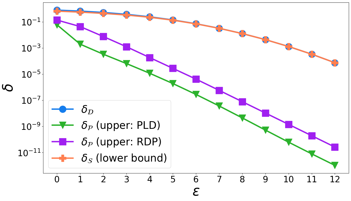
Appendix A Additional Evaluations
A.1 vs for fixed and
We first plot vs for fixed and . We compute upper bounds on using Rényi differential privacy (RDP) as well as using privacy loss distributions (PLD). These accounting methods are provided in the open source Google dp_accounting library (Google’s DP Library., 2020).
In particular we consistently find that for small values of , provides almost no improvement over , and has that is significantly larger than .
-
•
In Figure 4, we set and number of steps . In particular, for , (as per PLD accounting) and (as per RDP accounting), whereas on the other hand, and .
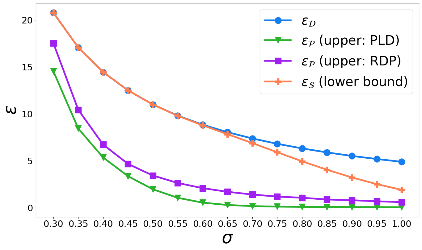
Figure 4: , upper bounds on and a lower bound on for varying and fixed and . -
•
In Figure 5, we set and number of steps . In particular, for , (as per PLD accounting) and (as per RDP accounting), whereas on the other hand, and .
A.2 vs for fixed and .
Next, we plot vs for fixed and . We compute upper bounds on using Rényi differential privacy (RDP) as well as using privacy loss distributions (PLD).
In particular when is closer to , we find that our lower bound on is distinctly smaller than , but still significantly larger than .
-
•
In Figure 6, we set and number of steps . In particular, while (as per PLD accounting) and (as per RDP accounting), we have that and .
For , we find the upper bound using PLD accounting to be larger than the upper bound using Rényi DP accounting. This is attributable to the numerical instability in PLD accounting when is very small.
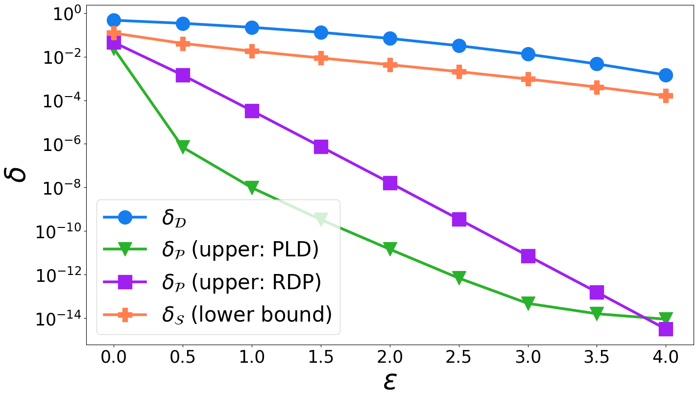
Figure 6: , upper bounds on and a lower bound on for varying and fixed and . -
•
In Figure 7, we set and number of steps . In particular, while (as per PLD accounting) and (as per RDP accounting), we have that and (last one not shown in plot).
For , we find the upper bound using PLD accounting appears to not decrease as much, which could be due to the numerical instability in PLD accounting when is very small.
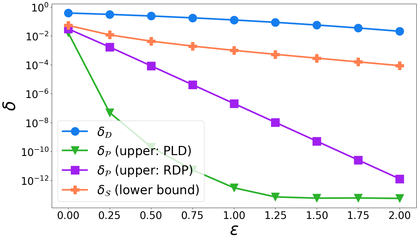
Figure 7: , upper bounds on and a lower bound on for varying and fixed and .
Appendix B Proof of Theorem 4.1
We make a simple observation that shuffling the dataset first cannot degrade the privacy guarantee of any mechanism.
Lemma B.1.
Fix a mechanism , and let be defined as for a random permutation over where . Then, if satisfies -, then also satisfies -.
Proof.
Consider any adjacent pair of dataset . For any permutation over , let and , and let and . It is easy to see that
If satisfies -, we have that for any measurable event , and any , it holds that , since and are also adjacent datasets. Hence we have that
Thus, also satisfies -DP. ∎
Proof of Theorem 4.1.
The proof follows by observing that if we choose in Lemma B.1, then is precisely the corresponding mechanism . ∎
Appendix C Additional proofs for vs
Proposition C.1.
For all and distributions , . And hence and equality can occur only if or .
Proof.
Recall that is the total variation distance between and , which has the following characterization where is a coupling such that . Given any coupling for , we construct a coupling of by sampling independently according to the coupling . From this, we have
By taking the infimum over all such that , we arrive at the desired bound. ∎
We also note that a simple observation that for all , the hockey stick divergence is a -Lipschitz in .
Proposition C.2.
For , it holds that
Proof.
We have that
∎