A family of Chatterjee’s correlation coefficients and their properties
Abstract
Quantifying the strength of functional dependence between random scalars and is an important statistical problem. While many existing correlation coefficients excel in identifying linear or monotone functional dependence, they fall short in capturing general non-monotone functional relationships. In response, we propose a family of correlation coefficients , characterized by a continuous bivariate function and a function . By offering a range of selections for and , encompasses a diverse class of novel correlation coefficients, while also incorporates the Chatterjee’s correlation coefficient (Chatterjee, , 2021) as a special case. We prove that converges almost surely to a deterministic limit as sample size approaches infinity. In addition, under appropriate conditions imposed on and , the limit satisfies the three appealing properties: (P1). it belongs to the range of ; (P2). it equals if and only if is a measurable function of ; and (P3). it equals if and only if is independent of . As amplified by our numerical experiments, our proposals provide practitioners with a variety of options to choose the most suitable correlation coefficient tailored to their specific practical needs.
Keywords: functional dependence, correlation coefficient, almost-surely convergence, central limit theorem, rank-based correlation.
1 Introduction
Measuring the strength of functional dependence between two random scalars and is a fundamental problem in statistics with broad scientific implications. In explicit statistical terms, the objective is to formulate a straightforward dependence estimate , wherein a higher value of indicates a stronger dependence of on . Ideally, attains its maximum value if and only if , where represents an arbitrary non-random measurable function. Across the extensive literature spanning the past century that focuses on quantifying pairwise associations, the majority of proposals have been primarily crafted for identifying linear/monotonic dependence patterns or testing independence, including the classical Pearson’s correlation coefficient, Spearman’s , and Kendall’s , as well as the distance correlations (Székely et al., , 2007; Székely and Rizzo, , 2009; Wang et al., , 2015), rank correlations (Drton et al., , 2020; Weihs et al., , 2018; Bergsma and Dassios, , 2014; Shi et al., , 2022), copula-based correlations (Schweizer and Wolff, , 1981; Chang et al., , 2016; Lopez-Paz et al., , 2013; Zhang, , 2019), binning-based correlations (Heller et al., , 2012; Kinney and Atwal, , 2014; Ma and Mao, , 2019), among many others. While for measuring the amount of general functional dependence where is possibly to be non-monotone, these approaches typically fall short in delivering meaningful and efficacious assessments.
1.1 Chatterjee’s correlation coefficient
The recent genius work of Chatterjee, (2021) has attracted very much attention. It proposed a new elegant correlation coefficient that effectively measures the extent of functional dependence under arbitrary functions. Given the data copies with , the Chatterjee’s correlation coefficient has a very simple expression:
| (1.1) |
where are reordered pairs of data such that , and represents the rank of among all ’s. The denominator term , acting as a normalization statistic, equals if there are no ties among ’s, and has a slightly altered expression in the presence of ties among ’s. Despite its simple non-parametric form, the most compelling feature of Chatterjee’s correlation coefficient is its almost-surely convergence to a limit , which satisfies the following three desirable properties:
-
(P1)
(Normalization). , for all distributions of .
-
(P2)
Perfect dependence. (reaches its maximum) if and only if there is a measurable function , such that almost surely.
-
(P3)
D-Consistency. (reaches its minimum) if and only if and are independent.
These three properties of , as first introduced by a prior work (Dette et al., , 2013), appear to be so strong that none of the preceding correlation measures can simultaneously fulfill all of them. In particular, the perfect dependence property (P2) stands as a distinguished characteristic of Chatterjee’s correlation coefficient, granting extraordinary capability in reflecting functional dependence. Several other correlation coefficients share the property of being maximized when is satisfied, including the maximal correlation coefficient (Rényi, , 1959), the maximum information coefficient (Reshef et al., , 2011), and the Hellinger correlation (Geenens and Lafaye de Micheaux, , 2022). But the converse is not true: they may also achieve maximum values when and exhibit noisy or non-functional relationships. Consequently, their identification of functional dependence can sometimes be inaccurate and misleading.
1.2 Motivation
We first present an intuitive rationale for the efficacy of Chatterjee’s correlation coefficient (1.1). One ingenuous aspect of (1.1) resides in the formulation of the numerator term . Here, is noted for quantifying the degree of variation between two consecutive ’s. Considering that the pairs are rearranged based on the order of values, the variation between two consecutive and tends to be small when the dependence of on is significant. Conversely, a greater variation is likely to occur when exhibits greater independence from . Therefore, achieving the maximum or minimum of (1.1) fundamentally relies on the dependence level between and .
This motivates a natural conjecture regarding potential extensions of Chatterjee’s correlation coefficient: replacing the term in (1.1) by other types of metrics on the degree of variation between and may still be effective for measuring functional dependence. This paper is dedicated to conducting a detailed investigation into this interesting question.
1.3 Our contributions
We propose a new correlation coefficient
| (1.2) |
with being a monotone univariate function, and being a non-negative continuous bivariate function, satisfying for . To enhance identifiability, we further restrict to be a cumulative distribution function (). The denominator serves as a normalization statistic, whose explicit expression will be presented later in Section 2. Comparing (1.2) with (1.1), the term in (1.2) is an extension of the corresponding term in (1.1), capable for quantifying the degree of variation between and . With a variety of choices for and functions, encompasses a wide family of new correlation coefficients that have not been previously explored in existing literature. It is noticeable that the Chatterjee’s correlation coefficient (1.1) corresponds to a special case of in (1.2) when taking , and as the empirical of ’s.
This paper seeks to provide answers to the fundamental questions concerning the asymptotic behaviors and limit properties of , which can be contingent upon the selection of and . We obtain a series of valuable results as outlined below.
-
1.
converges almost surely to a limit .
-
2.
The limit satisfies the perfect dependence property (P2), under mild regularity conditions on and .
-
3.
The limit as long as and are independent. Moreover, a central limit theorem is established for in the case where and are independent.
-
4.
We establish the necessary and sufficient condition for to satisfy all properties (P1)–(P3). Specifically, we delineate the set comprising continuous bivariate functions, wherein possesses properties (P1)–(P3) if and only if . Our findings reveal that the set is extensive, encompassing a diverse array of common bivariate functions.
-
5.
While the coefficient is initially formulated using deterministic and functions, we also allow taking as the empirical of ’s. In this scenario, becomes a rank-based correlation coefficient, for which the majority of the above four results are still valid.
The above results admit the existence of a wide family of new correlation coefficients that have theoretically-backed capability in measuring functional dependence between bivariate random variables. When dealing with real-world problems, our can better cater to practical needs by adapting and functions in a manner tailored to specific purposes. This flexibility contrasts with the constrained structure of the Chatterjee’s correlation coefficient. Extensive numerical experiments in Sections 5 and 6 lend empirical support to the practical efficacy of our proposals.
Outline of the paper.
Section 2 formally presents our correlation coefficient alongside its fundamental asymptotic properties. Section 3 demonstrate the necessary and sufficient condition for achieving all desired properties (P1)–(P3). Section 4 investigate the properties of the rank-based variant of when taking . Section 5 conducts extensive simulations for accessing the proposed correlation coefficient. Section 6 showcases an application of our correlation coefficient on a real-world dataset. Section 7 briefly concludes. Proofs of theorems are collected in the Supplementary Material.
Notations.
For integer , let be samples of in the probability space . Denote by the reordered pairs of samples such that . If there are ties among ’s, breaking the ties uniformly at random in this ordering. Let denote the indicator operator. Let and be the ’s of and respectively, and let be the empirical of ’s. Denote by the c.d.f of standard normal distribution. Denote by and the distribution laws of and . Let (or for short) denote the conditional law of given . For the existence of , refer to Theorem 2.1.22 and Exercise 4.1.18 in Durrett, (2019) (also see Lemma 1 in the Supplementary Material). Let and denote convergence in probability and in distribution respectively. For simplicity, the term “almost surely” is abbreviated as “” in case needed.
2 The new family of correlation coefficients
In this section, we formally present the formulation of our proposed correlation coefficient along with its fundamental properties. Throughout the paper, we assume that neither nor is a constant.
Definition 1 (New correlation coefficient).
For a non-negative continuous bivariate function satisfying for all , and a function , define the variation statistic
and the normalization statistic
The new correlation coefficient is defined as:
In case that , we set .
As previously mentioned in Section 1.3, the numerator term is designed to measure the degree of variation between consecutive ’s. The denominator term serves as a normalization statistic, ensuring that tends towards zero once if and are independent. Theorem 1 shows that converges almost surely to a deterministic constant as approaches infinity.
Theorem 1 (Convergence of correlation coefficient).
As , we have the following three convergence results:
the variation statistic converges a.s. to the limit
the normalization statistic converges a.s. to the limit
and the correlation coefficient converges a.s. to the limit
| (2.1) |
In case that , we set .
Throughout the paper, we call the population-level deterministic quantity the “correlation measure”, to distinguish it from its consistent empirical estimator which is called the “correlation coefficient”. Several remarks are provided in order.
Remark 2.1.
The new correlation coefficient requires no need for estimating probability densities, characteristic functions or mutual information, and it could be simply computed with a time complexity of . Moreover, and in are both prespecified deterministic functions, without the need of being tuned or estimated from the observed data.
Remark 2.2.
Remark 2.3.
Theorem 1 is almost assumption-free on and , except that is required to be continuous (as specified in Definition 1). This continuity condition for is vital for establishing Theorem 1. Lemma A.6 in Appendix A of the Supplementary Material shows a trivial example of a discontinuous for which does not converge to .
Remark 2.4.
Remark 2.5.
From our definition, it is noted that or fully depends on the functions and , yet this relationship is not “identifiable”. In other words, for distinct pairs of functions and , and could be identical correlation coefficients, provided that the composite functions and are the same. However, treating and separately is intentional, because and have different influences on the properties of the correlation coefficient. Such design of separate and not only facilitates further theoretical derivations, but also provides more concrete guidelines for constructing the correlation coefficients in real practice.
Remark 2.6.
Note that the function in is not required to be symmetric, which provides more flexibility. While for non-symmetric , the correlation measure in (2.1) remains unchanged if replacing this with the symmetric . Thus, when it turns to study the properties of , assuming to be symmetric will not lose generality. For convenience, we assume that is symmetric in the remainder of paper (refer to condition (C1)).
2.1 Perfect dependence property
For to serve as a reliable measure for the strength of functional dependence, one of the most desirable properties is the perfect dependence property (P2). Theorem 2 verifies that indeed possesses property (P2), provided that and satisfy the regularity conditions below.
-
(C1)
(Regularity condition on ). is a non-negative continuous symmetric function, satisfying , and for all .
-
(C2)
(Regularity condition on ). is a continuous and strictly-increasing function.
Theorem 2 (Properties of correlation measure).
For the above results, we give some remarks.
Remark 2.7.
Remark 2.8.
The main purpose for imposing the regularity conditions (C1)and (C2), is to ensure that is non-zero for any distinct . This further admits the necessity part of property (P2) in Theorem 2. If there exists distinct such that , then any random variable with the support would lead to and , which violates property (P2). Note that condition (C2) is satisfied if is a of some continuous random variable with support of .
Remark 2.9.
The property (P3)′ in Theorem 2, which is called the “I-consistency” property (Weihs et al., , 2018), corresponds to the sufficiency part of the “D-consistency” property (P3). Its proof can be seen as follows. If and are independent, then the conditional probability measure becomes for all . This gives that
which yields .
2.2 Central limit theorem
Measuring the amount of functional dependence is the major motivation for devising the correlation coefficient , while testing independence is not our initial focus. In particular, the correlation measure under the mild regularity conditions (C1) and (C2) satisfies the I-consistency property (P3)′, whereas the stronger D-consistency property (P3) will be derived in the next Section 3, after imposing further restrictions on . But still, we derive the central limit theorem for under independent and , suggesting its potential utility for conducting independence tests if desired.
Theorem 3 (CLT of under independence).
The asymptotic variance in Theorem 3 could be consistently estimated via constructing U-statistics on ’s; see details in Lemma A.13 in Appendix A of the Supplementary Material. In the special case of , , and being continuous, we have , which coincides with the variance in Chatterjee, (2021) [Theorem 2.2]. Also see Theorem 6 and Remark 4.1 in Section 4 for more related discussions.
3 Pursuing all properties (P1)–(P3)
Owning the perfect dependence property (P2), the family of correlation coefficients and satisfies conditions (C1) and (C2) are readily capable for measuring strength of dependence of on . To explore further understandings for the correlation coefficient, a natural question arises: for which cases of and does the corresponding correlation measure satisfy all the three desirable properties (P1)–(P3)? This section unveils the answer to this question.
3.1 Pursuing property (P1)
We first inspect the “normalization property” (P1). From the definition of correlation measure in (2.1), achieving property (P1) means that the difference is non-negative under any distributions of . Proposition 1 shows that this is achieved if and only if an additional condition (C3) is imposed on function .
-
(C3)
(Equivalence condition on for achieving (P1)). There exists a continuous positive-definite symmetric function , such that
(3.1)
Here, we call a symmetric bivariate function “positive-definite”, if for any real numbers and with , holds.
Proposition 1 (Necessary and sufficient condition for property (P1)).
Remark 3.1.
We provide some sketch of proof for Proposition 1. A closer inspection on and in Theorem 1 yields a useful identity:
Note that the double integral in the square bracket is symmetric with respect to and , with being its integral kernel. Thus, any negative-definite function would guarantee the positiveness of this double integral. This partly reflects why in (3.1) should include a term “”, which is negative-definite. After incorporating into , the purpose for adding the other two terms and is to ensure that is nonnegative and is satisfied for all . For more details, refer to Lemmas B.2 and B.3 in Appendix B of the Supplementary Material.
3.2 Pursuing properties (P1)–(P3)
Combining the results in Theorem 2 and Proposition 1, we have derived the necessary and sufficient condition such that satisfies properties (P1), (P2), and (P3)′. As long as the normalization property (P1) and the “I-consistency” property (P3)′ are both achieved, is guaranteed to attain its minimum value of under independent and . To fulfill all the three desired properties (P1)–(P3), the last step is to upgrade property (P3)′ to property (P3). That is, we just need to ensure that there exists no dependent and such that . This is done by adding an further condition (C4) on the positive-definite function in (3.1).
-
(C4)
(Condition on ). is a continuous positive-definite symmetric function, such that for any two distinct probability measures and satisfying , the set is non-empty.
Accordingly, condition (C3) of is upgraded to the following condition (C5).
- (C5)
Theorem 4 verifies that condition (C5) is the necessary and sufficient condition on such that achieves all properties (P1)–(P3).
To satisfy condition (C4), needs to be a positive-definite function such that the mapping from a probability law to the univariate function is one-to-one. This is equivalent to saying that is a characteristic kernel function (Sriperumbudur et al., , 2011), as defined in the context of the reproducing kernel Hilbert space. Examples of satisfying condition (C4) includes:
-
(a)
, for , which gives ;
-
(b)
, for , which yields .
Refer to Fukumizu et al., (2008) for a variety of other functions that satisfy condition (C4).
To provide a concise overview, Corollary 1 summarizes the results in the previous Theorems 2, 4, and Proposition 1.
Corollary 1 (Summary of results).
Remark 3.2.
To illustrate each result in Corollary 1, we showcase the properties of with , for . Case (1): . Then satisfies condition (C5) with satisfying condition (C4). Thus, possesses all properties (P1), (P2) and (P3). Case (2): . Then satisfies condition (C3), with . Since this does not satisfy condition (C4), possesses properties (P1), (P2) and (P3)′, but violates (P3). Case (3): . Then does not satisfy condition (P1), because with is not positive-definite. Thus, possesses properties (P2) and (P3)′, but violates (P1) and (P3).
4 Rank-based correlation coefficients
As previously noted, the rank-based Chatterjee’s correlation coefficient (1.1) corresponds to our coefficient when taking and as the empirical of . This motivates us to investigate the rank-based correlation coefficient in Definition 2, which is a variant of the previous when letting .
Definition 2 (Rank-based correlation coefficient).
For , let be the rank of among all ’s. For a non-negative continuous bivariate function satisfying for all , define the variation statistic
| (4.1) |
and the normalization statistic
| (4.2) |
The proposed rank-based correlation coefficient is defined as
In case that , we set .
It is noteworthy that all the theorems in previous sections are derived for with deterministic and , while the properties of the rank-based coefficient with non-deterministic remains unexplored. In our context, it is important to note that the empirical differs fundamentally from a typical in Definition 1. First, from an asymptotic standpoint, is a random function depending on the sample ’s and sample size , whereas is deterministic and independent from . This disparity significantly impacts the derivation of asymptotic theories. Second, in its nature is a piecewise-constant function, which obviously violates the continuity assumption for in condition (C2). For these reasons, the asymptotic properties of can not be directly inferred from the previous theorems, but need to be investigated separately and specifically.
Theorem 5 shows that also converges almost surely to a deterministic limit, provided that function is Lipschitz-continuous.
-
(C6)
(Lipschitz continuity condition on ). There exists a constant , such that , for any .
Theorem 5 (Convergence of rank-based correlation coefficient).
Moreover, when and are independent, the central limit theorem also holds for .
Theorem 6 (CLT of under independence).
Remark 4.1.
It is a well-known fact that follows a Unif distribution if is continuous. In such case, reduces to with . Owing to this expression, can be directly computed via numerical integrals, without the need of being estimated from the observed data. For example, when taking with , we have
where represents the gamma function. Letting yields , which agrees with the variance in Chatterjee, (2021) [Theorem 2.2].
4.1 Simplified rank-based coefficient under continuous
Note that for any continuous random variable . Therefore, if is continuous, the denominator term in (4.3) could be simplified as
| (4.5) |
which is a positive constant that does not rely on the distribution law of . In this scenario, the normalization statistic in (4.2), acting as consistent estimator for , could be simply replaced by the exact value . This gives rises to a simplified version of the rank-based correlation coefficient, as presented in Definition 3.
Definition 3 (Simplified rank-based correlation coefficient under continuous ).
A major appealing property for is its reduced computational cost compared to that of the original . This is because the normalization constant in does not rely on and could be directly computed from the integral (4.5). In fact, for many common functions, has simple close-form expressions. Take our previous examples of in Section 3.2, if for , then ; and if for , then . Without the need of evaluating the normalization statistic, the computational complexity of is reduced from to . Corollary 2 ensures that preserves all the asymptotic properties of in Theorems 5 and 6.
Corollary 2 (Consistency and CLT for simplified correlation coefficient).
To conclude, achieves the same nice asymptotic properties as , but with much reduced computational expense. Therefore, is a more efficient alternative to , if knowing that ’s take values in continuous support.
4.2 Properties of correlation measure
This subsection investigates the properties of correlation measure , which is the limit of the rank-based correlation coefficient or its simplified version . A comparison between the correlation measures in (4.4) and in (2.1) gives that , that is, coincides with when substituting . One may speculate that also preserves similar properties of as presented in Theorems 2, 4, and Proposition 1. Again, this needs to be reexamined, as we should not simply regard as a special case of . For all previous theorems related to , is assumed to be a fixed function that does not depend on the sample distribution and satisfies the regularity condition (C2). In contrast, not only depends on the sample distribution, but also possibly violates the required regularity condition (C2). We stress that our investigation into properties (P1)–(P3) encompasses all possible probability distributions of , only except for constant or .
To proceed, we first present conditions (C4)′ and (C5)′, which are modified version of conditions (C4) and (C5) in Section 3.2.
-
(C4)′
(Modified condition on ). is a continuous positive-definite symmetric function, such that for any two distinct probability measures and satisfying , the set is non-empty.
- (C5)′
Note that the difference between conditions (C4)′ and (C4) is minor: the open interval in condition (C4) is modified to be the wider half-open interval in condition (C4) (i.e., “” in (C4) is revised to be “” in (C4)′). Therefore, the revised conditions (C4)′ and (C5)′ are slightly stronger than the previous conditions (C4) and (C5). Theorem 7 verifies that possesses similar properties to .
Theorem 7 (Properties of correlation measure ).
In comparison with the previous Corollary 1 for , most results in Theorem 7 for remain unchanged. The only exception is that we solely confirmed condition (C5)′ as the sufficiency condition for attaining all properties (P1)–(P3), leaving uncertain whether it is also the necessary condition. This poses an open question for future resolution.
4.3 Other related works
There are several recent works that extended the Chatterjee’s correlation coefficient in different directions. Azadkia and Chatterjee, (2021) proposed a correlation coefficient based on for measuring the conditional dependence of on given , and accordingly designed a new variable selection algorithm. Lin and Han, 2022a proved the CLT for Chatterjee’s correlation coefficient under arbitrary distributions of . Auddy et al., (2021), Bickel, (2022) and Shi et al., (2021) conducted power analyses for under a family of alternatives. Lin and Han, 2022b extended to enhance power for independence tests, by incorporating multiple nearby ranks. Generalizations of to multi-dimensional spaces were proposed in Huang et al., (2022), Gamboa et al., (2022), and Fuchs, (2024). Scientific applications of across various fields could be found in Sadeghi, (2022), Zarei et al., (2023), and Nurdiati et al., (2022). Refer to Chatterjee, (2022) for a comprehensive review of recent follow-up works. While these works focus on various topics such as independence test, power analysis, variable selection, and high-dimensional extensions, our research takes a distinct approach. We concentrate on tackling the fundamental task of quantifying functional dependence between two random scalars — an objective that aligns with the original intention of the Chatterjee’s work. In pursuit of this goal, we have developed enhanced alternatives to the Chatterjee’s correlation coefficient. As we will later show in numerical examples in Section 5, with appropriate choices of and functions, our newly proposed correlation coefficients are more sensitive in identifying perfect or near-perfect functional dependence than the Chatterjee’s correlation coefficient.
5 Simulation studies
In this section, we evaluate the performance of our proposed correlation coefficients via simulations on synthetic data.
5.1 Set-up
For generating the synthetic data , we adopt the following three models as used in section 4 of Chatterjee, (2021):
- Model 1 (Linear):
-
- Model 2 (Quadratic):
-
- Model 3 (Sinusoidal):
-
In each of the three models mentioned above, we set . Additionally, is the Gaussian noise independent of , and represents the noise magnitude. With a slight abuse of notation, we also allow taking , which corresponds to the scenario where is pure noise.
We access the performance of the correlation coefficient in Definition 1 with being the of distribution, as well as the simplified rank-based correlation coefficient in Definition 3. For both of and , the bivariate function is specified from the following five cases: (1) ; (2) ; (3) ; (4) ; and (5) . According to Corollary 1 and Theorem 7, the correlation measures and can possess different properties of (P1)–(P3) contingent upon the specific functions. Specifically, and lead to properties (P1), (P2), and (P3); and result in properties (P1), (P2), and (P3)′; and yields properties (P2) and (P3)′. These functions all give rise to the perfect dependence property (P2), indicating the validity of the corresponding correlation coefficients for detecting arbitrarily-shaped functional dependence.
5.2 Illustrative example
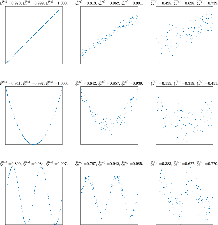
Figure 1 provides an illustrative example on the performance of simplified rank-based correlation coefficient , with , or . Note that with coincides with the Chatterjee’s correlation coefficient in (1.1), which serves as a benchmark for method comparisons. Across all models, the three correlation coefficients exhibit higher values when the noise level is lower. In each panel of Figure 1, the three correlation coefficients consistently follow this order: . This suggests that and are more sensitive than in identifying functional dependence, especially under the case of winding-shaped Models 2 and 3. In particular, for the noise-free case , all three correlation coefficients are expected to converge to according to the perfect dependence property (P2). It is observed that and are much closer to (with the largest difference ) than (with the largest difference ). This indicates that and have higher convergence speed than , or in other words, and can attain enhanced detection results with a reduced sample size requirement. This simulation example reveals that among our proposed family of correlation coefficients, some with appropriately-chosen functions may have better practical abilities for detecting functional relationship than the benchmark Chatterjee’s correlation coefficient.
5.3 Comparison with other correlation coefficients
To provide a more comprehensive evaluation, we compare our correlation coefficient with some other methods, which includes the Peason’s correlation coefficient, the Spearman’s , the distance correlation (abbreviated as “dCorr”) in Székely et al., (2007), the power-enhanced Chatterjee’s correlation coefficient in Lin and Han, 2022b (abbreviated as “LH”, with the number of nearest neighbor ), and the Maximal Information Coefficient (MIC) in Reshef et al., (2011).
Under the linear Model 1, all methods exhibit similar performances; therefore, the results are omitted. Tables 1 and 2 report the values of correlation coefficients of each method under Models 2 and 3 respectively. As the sample size grows from to , the mean values of each correlation coefficient slightly changes, whereas the standard deviations become closer to zero. This implies a trend of asymptotic convergence for and , which agrees with our Theorems 1 and 5. Under both the two models, our proposed correlation coefficients and distinguish themselves from other methods by clearly reflecting the amount of functional dependence between and . It is seen that and are approximately equal to under perfect dependence (i.e., ), then decrease as the noise level grows, and finally approaches to zero when (i.e., ) consists of pure noise. The MIC shows a similar trend, but it does not approach zero closely when the noise level goes to infinity, as it has the largest value among all methods under the case of . Though the MIC is theoretically guaranteed to converge to zero (i.e., satisfying property (P3)′) for independent and , our simulation results indicate that its convergence speed is significantly slower than other methods. The LH correlation coefficient is comparable to the Chatterjee’s correlation coefficient when the sample size is large (), but exhibits inferior performance when the sample size is small (). The distance correlation “dCorr” shows a trend of decreasing to zero as grows, while it is far away from reaching for the noise-free case (). The Pearson correlation coefficient and Spearman’s fail to identify significant functional relationships in both models, as they are either negative or close to zero even under strong functional dependence (). For the comparison between the two proposed coefficient and , they exhibit similar values when using identical functions. Among the five selected functions, , and yield higher values of correlation coefficients than and do, especially when the functional dependence is strong (). This also agrees with the previous results reflected in Figure 1.
| Method | |||||||||||||
|---|---|---|---|---|---|---|---|---|---|---|---|---|---|
| n=100 | n=500 | n=2000 | n=100 | n=500 | n=2000 | n=100 | n=500 | n=2000 | n=100 | n=500 | n=2000 | ||
| 0.943 | 0.989 | 0.997 | 0.674 | 0.680 | 0.680 | 0.126 | 0.145 | 0.143 | 0.004 | -0.003 | -0.001 | ||
| (0.25) | (0.03) | (0.00) | (3.20) | (1.66) | (0.92) | (6.26) | (2.94) | (1.92) | (6.16) | (2.62) | (1.72) | ||
| 0.995 | 1.000 | 1.000 | 0.890 | 0.893 | 0.893 | 0.221 | 0.251 | 0.248 | -0.000 | -0.003 | -0.002 | ||
| (0.08) | (0.00) | (0.00) | (2.00) | (1.03) | (0.57) | (10.01) | (4.49) | (2.97) | (9.57) | (4.07) | (2.88) | ||
| 0.999 | 1.000 | 1.000 | 0.961 | 0.963 | 0.962 | 0.296 | 0.332 | 0.330 | -0.008 | -0.002 | -0.003 | ||
| (0.03) | (0.00) | (0.00) | (1.04) | (0.54) | (0.29) | (13.22) | (5.81) | (3.73) | (12.90) | (5.53) | (3.88) | ||
| 0.994 | 1.000 | 1.000 | 0.897 | 0.902 | 0.901 | 0.235 | 0.264 | 0.262 | -0.003 | -0.003 | -0.002 | ||
| (0.10) | (0.00) | (0.00) | (1.90) | (0.93) | (0.51) | (10.15) | (4.46) | (2.91) | (9.65) | (4.20) | (2.93) | ||
| 0.939 | 0.988 | 0.997 | 0.653 | 0.659 | 0.659 | 0.111 | 0.128 | 0.127 | 0.005 | -0.003 | -0.001 | ||
| (0.25) | (0.03) | (0.00) | (3.27) | (1.70) | (0.93) | (5.77) | (2.73) | (1.76) | (5.53) | (2.36) | (1.49) | ||
| 0.941 | 0.988 | 0.997 | 0.645 | 0.660 | 0.664 | 0.134 | 0.155 | 0.155 | 0.004 | -0.003 | 0.000 | ||
| (Chatterjee) | (0.04) | (0.00) | (0.00) | (3.50) | (1.94) | (0.91) | (6.66) | (3.07) | (1.73) | (6.10) | (2.63) | (1.38) | |
| 0.997 | 1.000 | 1.000 | 0.859 | 0.865 | 0.869 | 0.225 | 0.257 | 0.257 | -0.000 | -0.003 | 0.000 | ||
| (0.03) | (0.00) | (0.00) | (2.90) | (1.59) | (0.71) | (10.27) | (4.47) | (2.54) | (9.52) | (4.08) | (2.16) | ||
| 1.000 | 1.000 | 1.000 | 0.938 | 0.941 | 0.943 | 0.292 | 0.331 | 0.331 | -0.008 | -0.002 | -0.001 | ||
| (0.01) | (0.00) | (0.00) | (2.04) | (1.08) | (0.47) | (12.85) | (5.48) | (3.05) | (12.84) | (5.54) | (2.84) | ||
| 0.996 | 1.000 | 1.000 | 0.816 | 0.822 | 0.827 | 0.200 | 0.239 | 0.241 | -0.008 | -0.004 | -0.000 | ||
| (0.04) | (0.00) | (0.00) | (4.06) | (2.20) | (0.97) | (10.22) | (4.53) | (2.51) | (9.61) | (4.00) | (2.13) | ||
| 0.927 | 0.985 | 0.996 | 0.593 | 0.609 | 0.614 | 0.113 | 0.132 | 0.132 | 0.005 | -0.003 | 0.000 | ||
| (0.05) | (0.00) | (0.00) | (3.65) | (2.02) | (0.96) | (5.93) | (2.79) | (1.56) | (5.48) | (2.36) | (1.23) | ||
| Pearson | -0.005 | -0.007 | 0.003 | 0.021 | 0.007 | 0.005 | -0.004 | -0.006 | -0.004 | 0.003 | 0.007 | -0.000 | |
| (12.98) | (5.04) | (2.42) | (12.10) | (5.83) | (2.72) | (11.08) | (4.51) | (2.39) | (8.65) | (4.75) | (2.33) | ||
| Spearman | -0.003 | -0.007 | 0.000 | 0.010 | 0.002 | 0.005 | -0.004 | -0.007 | -0.003 | 0.003 | 0.009 | -0.001 | |
| (14.46) | (5.64) | (2.67) | (12.91) | (5.96) | (3.27) | (12.02) | (4.81) | (2.38) | (8.63) | (4.65) | (2.41) | ||
| dCorr | 0.514 | 0.496 | 0.492 | 0.485 | 0.468 | 0.462 | 0.278 | 0.245 | 0.239 | 0.160 | 0.074 | 0.038 | |
| (2.82) | (1.04) | (0.46) | (2.65) | (1.05) | (0.53) | (4.37) | (1.75) | (0.91) | (3.15) | (1.68) | (0.90) | ||
| LH | 0.611 | 0.918 | 0.979 | 0.470 | 0.638 | 0.660 | 0.026 | 0.134 | 0.150 | -0.161 | -0.032 | -0.008 | |
| (0.00) | (0.00) | (0.00) | (2.45) | (1.59) | (0.75) | (5.18) | (2.05) | (1.28) | (2.62) | (0.95) | (0.46) | ||
| MIC | 1.000 | 1.000 | 1.000 | 0.876 | 0.847 | 0.813 | 0.342 | 0.285 | 0.240 | 0.238 | 0.163 | 0.107 | |
| (0.00) | (0.00) | (0.00) | (6.26) | (2.96) | (1.57) | (6.27) | (2.63) | (1.59) | (3.62) | (1.40) | (0.51) | ||
| Method | |||||||||||||
|---|---|---|---|---|---|---|---|---|---|---|---|---|---|
| n=100 | n=500 | n=2000 | n=100 | n=500 | n=2000 | n=100 | n=500 | n=2000 | n=100 | n=500 | n=2000 | ||
| 0.907 | 0.981 | 0.995 | 0.840 | 0.874 | 0.876 | 0.462 | 0.468 | 0.470 | 0.004 | -0.003 | -0.001 | ||
| (0.37) | (0.03) | (0.01) | (1.13) | (0.56) | (0.36) | (5.37) | (2.50) | (1.41) | (6.16) | (2.62) | (1.72) | ||
| 0.985 | 0.999 | 1.000 | 0.970 | 0.983 | 0.984 | 0.686 | 0.693 | 0.696 | -0.000 | -0.003 | -0.002 | ||
| (0.18) | (0.00) | (0.00) | (0.44) | (0.15) | (0.10) | (6.06) | (2.76) | (1.54) | (9.57) | (4.07) | (2.88) | ||
| 0.997 | 1.000 | 1.000 | 0.993 | 0.997 | 0.998 | 0.803 | 0.809 | 0.812 | -0.008 | -0.002 | -0.003 | ||
| (0.11) | (0.00) | (0.00) | (0.20) | (0.03) | (0.02) | (5.65) | (2.58) | (1.39) | (12.90) | (5.53) | (3.88) | ||
| 0.985 | 0.999 | 1.000 | 0.969 | 0.982 | 0.983 | 0.677 | 0.685 | 0.687 | -0.003 | -0.003 | -0.002 | ||
| (0.18) | (0.00) | (0.00) | (0.52) | (0.16) | (0.10) | (5.92) | (2.66) | (1.63) | (9.65) | (4.20) | (2.93) | ||
| 0.890 | 0.977 | 0.994 | 0.811 | 0.850 | 0.852 | 0.411 | 0.417 | 0.419 | 0.005 | -0.003 | -0.001 | ||
| (0.39) | (0.03) | (0.00) | (1.23) | (0.64) | (0.39) | (5.15) | (2.42) | (1.36) | (5.53) | (2.36) | (1.49) | ||
| 0.886 | 0.976 | 0.994 | 0.784 | 0.833 | 0.837 | 0.446 | 0.459 | 0.462 | 0.004 | -0.003 | 0.000 | ||
| (Chatterjee) | (0.18) | (0.01) | (0.00) | (1.71) | (0.86) | (0.41) | (4.88) | (2.36) | (1.23) | (6.10) | (2.63) | (1.38) | |
| 0.985 | 0.999 | 1.000 | 0.950 | 0.969 | 0.971 | 0.675 | 0.687 | 0.691 | -0.000 | -0.003 | 0.000 | ||
| (0.13) | (0.00) | (0.00) | (0.80) | (0.32) | (0.16) | (5.81) | (2.69) | (1.35) | (9.52) | (4.08) | (2.16) | ||
| 0.997 | 1.000 | 1.000 | 0.988 | 0.994 | 0.994 | 0.797 | 0.808 | 0.812 | -0.008 | -0.002 | -0.001 | ||
| (0.07) | (0.00) | (0.00) | (0.32) | (0.11) | (0.05) | (5.58) | (2.59) | (1.26) | (12.84) | (5.54) | (2.84) | ||
| 0.983 | 0.999 | 1.000 | 0.944 | 0.965 | 0.966 | 0.663 | 0.678 | 0.681 | -0.008 | -0.004 | -0.000 | ||
| (0.14) | (0.00) | (0.00) | (1.13) | (0.53) | (0.23) | (6.51) | (3.12) | (1.37) | (9.61) | (4.00) | (2.13) | ||
| 0.860 | 0.970 | 0.992 | 0.742 | 0.799 | 0.803 | 0.392 | 0.405 | 0.408 | 0.005 | -0.003 | 0.000 | ||
| (0.22) | (0.01) | (0.00) | (1.94) | (0.99) | (0.48) | (4.70) | (2.29) | (1.21) | (5.48) | (2.36) | (1.23) | ||
| Pearson | -0.380 | -0.385 | -0.391 | -0.381 | -0.380 | -0.387 | -0.311 | -0.316 | -0.318 | 0.003 | 0.007 | -0.000 | |
| (7.67) | (3.44) | (1.69) | (7.38) | (3.35) | (1.68) | (8.08) | (3.40) | (1.93) | (8.65) | (4.75) | (2.33) | ||
| Spearman | -0.363 | -0.369 | -0.376 | -0.365 | -0.366 | -0.375 | -0.317 | -0.326 | -0.326 | 0.003 | 0.009 | -0.001 | |
| (8.71) | (3.98) | (1.96) | (8.16) | (4.00) | (1.85) | (9.08) | (3.74) | (2.09) | (8.63) | (4.65) | (2.41) | ||
| dCorr | 0.440 | 0.431 | 0.432 | 0.442 | 0.426 | 0.428 | 0.371 | 0.355 | 0.354 | 0.160 | 0.074 | 0.038 | |
| (4.90) | (2.29) | (1.16) | (4.56) | (2.27) | (1.19) | (5.24) | (2.26) | (1.42) | (3.15) | (1.68) | (0.90) | ||
| LH | 0.269 | 0.826 | 0.955 | 0.262 | 0.750 | 0.823 | 0.128 | 0.411 | 0.451 | -0.161 | -0.032 | -0.008 | |
| (2.19) | (0.18) | (0.02) | (2.41) | (0.63) | (0.33) | (3.70) | (1.74) | (0.98) | (2.62) | (0.95) | (0.46) | ||
| MIC | 1.000 | 1.000 | 1.000 | 0.990 | 0.995 | 0.979 | 0.671 | 0.640 | 0.608 | 0.238 | 0.163 | 0.107 | |
| (0.00) | (0.00) | (0.00) | (1.82) | (0.78) | (0.82) | (8.53) | (3.58) | (2.13) | (3.62) | (1.40) | (0.51) | ||
For a more intuitive presentation of results, Figure 2 visualizes the trend of correlation coefficient with growing noise magnitude for the six selected methods under Model 1 and Model 2. Among these methods, with proves to be the most desirable correlation coefficient under both models, as it exhibits the highest value in scenarios when the noise is small and dependence is strong, while rapidly approaching zero as and become more independent.

6 Real data experiment
The S&P 500, also known as the Standard and Poor’s 500, serves as a pivotal stock market index overseeing the performance of approximately 500 of the largest companies listed on United States stock exchanges. A primary objective for financial quant analysts involves examining the longitudinal trends and stability exhibited by these stock prices, which is crucial for refining effective trading strategies. Our proposed correlation coefficient is poised to meet this objective. Specifically, our correlation coefficient is intended for assessing the extent of functional dependence between each stock price and the temporal variable : higher dependence signifies a more stable trend in stock price, while lower dependence corresponds to augmented volatility and unpredictability within the stock. As an illustrative instance, our experiment scrutinizes the short-term volatility of the opening prices of the 504 stocks encompassed by the S&P 500 index over a consecutive 50-day trading span from November 27, 2017, to February 7, 2018. The dataset is accessible at https://www.kaggle.com/datasets/camnugent/sandp500.
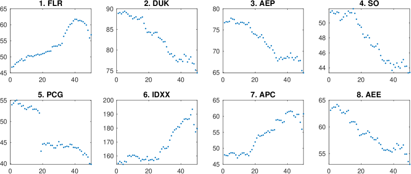
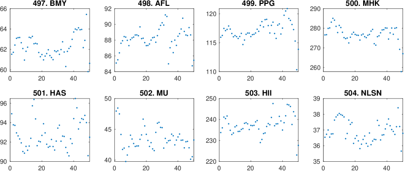
We first employ in (1.2), with function taking . For the function, we adopt , where and denote the mean and the standard deviation respectively of the observed sample , and is the of standard normal distribution. To show the efficacy of our method, we sort these 504 stocks based on the values of their corresponding correlation coefficients . Figures 3 and 4 display scatter plots of the stock prices for the top 8 stocks with the highest values and the bottom 8 stocks with the lowest values, respectively. In a stark contrast, the 8 stocks depicted in Figure 3 exhibit smooth changes over time, whereas the 8 stocks in Figure 4 demonstrate considerable fluctuations. Upon closer examination of the top 8 stocks in Figure 3, it is noticeable that certain stocks (e.g., DUK, AEP, PCG) follow a monotonic trend of changes, whereas others (e.g., FLR, IDXX, APC) exhibit smooth but relatively non-monotonic variations over time. This showcases the effectiveness of our correlation coefficient in identifying perfect functional dependence, regardless of whether this dependence is monotonic or not.
To draw a comparison, we also employ four other methods: our with function taking , the Chatterjee’s correlation coefficient, the MIC (Reshef et al., , 2011), and the distance correlation (Székely et al., , 2007). Table 3 displays the values of each correlation coefficient for the top 8 stocks (selected by ). The coefficient exhibits slight variation compared to , yet maintains nearly identical rankings for the 8 selected stocks among the total 504 stocks. This suggests that transitioning from the function to in this context does not significantly alter the outcomes. The Chatterjee’s correlation coefficient, also represented by within our framework of simplified rank-based coefficient, displays more significant differences in rankings compared to . This outcome is not surprising, given that a significant portion of the 504 stocks exhibit very high correlation coefficient values for both and . Consequently, even a slight alteration in coefficient values may result in substantial changes in their respective rankings among all stocks. For the MIC, it turns out that 177 out of the total 504 stocks share a MIC value of in common, and 7 out of the 8 selected stocks in Table 3 has MIC of . Consequently, the MIC demonstrates limited utility as it fails to discern differences among many of these stocks. The distance correlation seems to be more sensitive at identifying monotonic relationships. However, for stocks like FLR and IDXX, which display non-monotonic functional dependence, the distance correlation tends to yield smaller values and lower ranks. Among the top 8 stocks in Figure 3, the fifth one PCG stands out notably. This is due to a significant price drop occurring around day 20, leading to the stock price’s relationship with time resembling more of a piecewise continuous function. We anticipate that our proposed correlation coefficient is able to identify such “piecewise smooth” functional relationships. As indicated by property (P2), our correlation coefficient is expected to yield the highest value when , where the function only needs to be measurable, but not necessarily to be continuous across the entire support of . Consequently, such special type of “piecewise smooth” functional dependence is successfully identified by our and , whereas it is overlooked by the other three approaches. In summary, this experiment highlights the effectiveness of our proposed correlation coefficient in real-world applications.
| Stock | Chatterjee | MIC | dCorr | |||||||
|---|---|---|---|---|---|---|---|---|---|---|
| value | rank | value | rank | value | rank | value | rank | value | rank | |
| FLR | 0.920 | 1 | 0.900 | 1 | 0.885 | 1 | 1.000 | 1 | 0.944 | 27 |
| DUK | 0.914 | 2 | 0.892 | 2 | 0.833 | 5 | 1.000 | 1 | 0.980 | 1 |
| AEP | 0.904 | 3 | 0.878 | 4 | 0.784 | 57 | 1.000 | 1 | 0.972 | 2 |
| SO | 0.902 | 4 | 0.876 | 5 | 0.772 | 92 | 1.000 | 1 | 0.971 | 6 |
| PCG | 0.902 | 5 | 0.885 | 3 | 0.738 | 178 | 0.925 | 244 | 0.891 | 99 |
| IDXX | 0.896 | 6 | 0.869 | 8 | 0.792 | 44 | 1.000 | 1 | 0.914 | 62 |
| APC | 0.896 | 7 | 0.871 | 6 | 0.803 | 29 | 1.000 | 1 | 0.960 | 16 |
| AEE | 0.894 | 8 | 0.869 | 7 | 0.826 | 11 | 1.000 | 1 | 0.962 | 13 |
7 Discussion
Inspired by the utility of Chatterjee’s correlation coefficient in measuring functional dependence, we proposed three new types of correlation coefficients: the original proposal in Definition 1, the rank-based variant in Definition 2 and its simplified version in Definition 3. We provide a systematic examination on the asymptotic properties of these coefficients, and demonstrate their capability for measuring functional dependence through both theoretical analysis and case studies.
Several issues warrant further investigation. First, how to select the the type of correlation coefficient , , or in a specific real-world problem? From our theoretical results, , , and have similar nice asymptotic properties; while in specific real applications, they may lead to notable differences. An example is that the two correlation coefficient and (i.e., the Chatterjee’s correlation coefficient), though with the identical functions, leads to notably different stock ranks in Table 3. Conceptually, is based on the ranks of , suggesting its greater robustness against outliers or abrupt changes; whereas is non-rank-based, enabling it to leverage more information from the distribution of sample. These distinct characteristics allow practitioners to select the type of correlation coefficient that best suits their specific requirements. Second, how to select and functions for our correlation coefficients? Again, our theoretical results provide guidances for selecting and , e.g., we derive the necessary and sufficient condition on to achieve all desirable properties (P1)–(P3). Yet the practical performance may differ with the theoretical expectations. For instance, with only possesses part of the three properties (P1)–(P3), but it demonstrates best practical performance in our simulation example, as reflected in Figure 2. In this regard, more practical guidance is needed for choosing and . Thirdly, exploring further theoretical results, such as the convergence rate of correlation coefficients and the central limit theorem under non-independent and , holds potential for future investigation.
References
- Auddy et al., (2021) Auddy, A., Deb, N., and Nandy, S. (2021). Exact detection thresholds for Chatterjee’s correlation. ArXiv preprint. Available at arXiv:2104.15140.
- Azadkia and Chatterjee, (2021) Azadkia, M. and Chatterjee, S. (2021). A simple measure of conditional dependence. The Annals of Statistics, 49(6):3070–3102.
- Bergsma and Dassios, (2014) Bergsma, W. and Dassios, A. (2014). A consistent test of independence based on a sign covariance related to Kendall’s tau. Bernoulli, 20(2):1006–1028.
- Bickel, (2022) Bickel, P. J. (2022). Measures of independence and functional dependence. ArXiv preprint. Available at arXiv:2206.13663.
- Chang et al., (2016) Chang, Y., Li, Y., Ding, A., and Dy, J. (2016). A robust-equitable copula dependence measure for feature selection. In Artificial Intelligence and Statistics, pages 84–92. PMLR.
- Chatterjee, (2021) Chatterjee, S. (2021). A new coefficient of correlation. Journal of the American Statistical Association, 116(536):2009–2022.
- Chatterjee, (2022) Chatterjee, S. (2022). A survey of some recent developments in measures of association. ArXiv preprint. Available at arXiv:2211.04702.
- Dette et al., (2013) Dette, H., Siburg, K. F., and Stoimenov, P. A. (2013). A copula‐based non‐parametric measure of regression dependence. Scandinavian Journal of Statistics, 40(1):21–41.
- Drton et al., (2020) Drton, M., Han, F., and Shi, H. (2020). High-dimensional consistent independence testing with maxima of rank correlations. The Annals of Statistics, 48(6):3206–3227.
- Durrett, (2019) Durrett, R. (2019). Probability: theory and examples, volume 49. Cambridge university press.
- Fuchs, (2024) Fuchs, S. (2024). Quantifying directed dependence via dimension reduction. Journal of Multivariate Analysis, 201:105266.
- Fukumizu et al., (2008) Fukumizu, K., Gretton, A., Schölkopf, B., and Sriperumbudur, B. K. (2008). Characteristic kernels on groups and semigroups. In Advances in Neural Information Processing Systems, volume 21. Curran Associates, Inc.
- Gamboa et al., (2022) Gamboa, F., Gremaud, P., Klein, T., and Lagnoux, A. (2022). Global sensitivity analysis: A novel generation of mighty estimators based on rank statistics. Bernoulli, 28(4):2345–2374.
- Geenens and Lafaye de Micheaux, (2022) Geenens, G. and Lafaye de Micheaux, P. (2022). The hellinger correlation. Journal of the American Statistical Association, 117(538):639–653.
- Heller et al., (2012) Heller, R., Heller, Y., and Gorfine, M. (2012). A consistent multivariate test of association based on ranks of distances. Biometrika, 100(2):503–510.
- Huang et al., (2022) Huang, Z., Deb, N., and Sen, B. (2022). Kernel partial correlation coefficient—a measure of conditional dependence. The Journal of Machine Learning Research, 23(1):9699–9756.
- Kinney and Atwal, (2014) Kinney, J. B. and Atwal, G. S. (2014). Equitability, mutual information, and the maximal information coefficient. Proceedings of the National Academy of Sciences, 111(9):3354–3359.
- (18) Lin, Z. and Han, F. (2022a). Limit theorems of Chatterjee’s rank correlation. ArXiv preprint. Available at arXiv:2204.08031.
- (19) Lin, Z. and Han, F. (2022b). On boosting the power of Chatterjee’s rank correlation. Biometrika, 110(2):283–299.
- Lopez-Paz et al., (2013) Lopez-Paz, D., Hennig, P., and Schölkopf, B. (2013). The randomized dependence coefficient. In Advances in Neural Information Processing Systems, volume 26. Curran Associates, Inc.
- Ma and Mao, (2019) Ma, L. and Mao, J. (2019). Fisher exact scanning for dependency. Journal of the American Statistical Association, 114(525):245–258.
- Nurdiati et al., (2022) Nurdiati, S., Sopaheluwakan, A., Septiawan, P., and Ardhana, M. R. (2022). Joint spatio-temporal analysis of various wildfire and drought indicators in Indonesia. Atmosphere, 13(10):1591.
- Reshef et al., (2011) Reshef, D. N., Reshef, Y. A., Finucane, H. K., Grossman, S. R., McVean, G., Turnbaugh, P. J., Lander, E. S., Mitzenmacher, M., and Sabeti, P. C. (2011). Detecting novel associations in large data sets. Science, 334(6062):1518–1524.
- Rényi, (1959) Rényi, A. (1959). On measures of dependence. Acta Mathematica Academiae Scientiarum Hungarica, 10(3-4):441–451.
- Sadeghi, (2022) Sadeghi, B. (2022). Chatterjee Correlation Coefficient: A robust alternative for classic correlation methods in geochemical studies- (including “TripleCpy” Python package). Ore Geology Reviews, 146:104954.
- Schweizer and Wolff, (1981) Schweizer, B. and Wolff, E. F. (1981). On nonparametric measures of dependence for random variables. The Annals of Statistics, 9(4):879–885.
- Shi et al., (2021) Shi, H., Drton, M., and Han, F. (2021). On the power of Chatterjee’s rank correlation. Biometrika, 109(2):317–333.
- Shi et al., (2022) Shi, H., Hallin, M., Drton, M., and Han, F. (2022). On universally consistent and fully distribution-free rank tests of vector independence. The Annals of Statistics, 50(4):1933–1959.
- Sriperumbudur et al., (2011) Sriperumbudur, B. K., Fukumizu, K., and Lanckriet, G. R. (2011). Universality, characteristic kernels and rkhs embedding of measures. The Journal of Machine Learning Research, 12(7).
- Székely and Rizzo, (2009) Székely, G. J. and Rizzo, M. L. (2009). Brownian distance covariance. The Annals of Applied Statistics, 3(4):1236–1265.
- Székely et al., (2007) Székely, G. J., Rizzo, M. L., and Bakirov, N. K. (2007). Measuring and testing dependence by correlation of distances. The Annals of Statistics, 35(6):2769–2794.
- Wang et al., (2015) Wang, X., Pan, W., Hu, W., Tian, Y., and Zhang, H. (2015). Conditional distance correlation. Journal of the American Statistical Association, 110(512):1726–1734.
- Weihs et al., (2018) Weihs, L., Drton, M., and Meinshausen, N. (2018). Symmetric rank covariances: a generalized framework for nonparametric measures of dependence. Biometrika, 105(3):547–562.
- Zarei et al., (2023) Zarei, A. R., Mokarram, M., and Mahmoudi, M. R. (2023). Comparison of the capability of the Meteorological and Remote Sensing Drought Indices. Water Resources Management, 37(2):769–796.
- Zhang, (2019) Zhang, K. (2019). Bet on independence. Journal of the American Statistical Association, 114(528):1620–1637.