UADA3D: Unsupervised Adversarial Domain Adaptation for 3D Object Detection with Sparse LiDAR and Large Domain Gaps

Abstract

In this study, we address a gap in existing unsupervised domain adaptation approaches on LiDAR-based 3D object detection, which have predominantly concentrated on adapting between established, high-density autonomous driving datasets. We focus on sparser point clouds, capturing scenarios from different perspectives: not just from vehicles on the road but also from mobile robots on sidewalks, which encounter significantly different environmental conditions and sensor configurations. We introduce Unsupervised Adversarial Domain Adaptation for 3D Object Detection (UADA3D). UADA3D does not depend on pre-trained source models or teacher-student architectures. Instead, it uses an adversarial approach to directly learn domain-invariant features. We demonstrate its efficacy in various adaptation scenarios, showing significant improvements in both self-driving car and mobile robot domains. Our code is open-source and will be available at the https://github.com/maxiuw/UADA3Drepository.

1 Introduction

LiDAR-based perception systems are essential for the safe navigation of autonomous vehicles such as self-driving cars [20] or mobile robots [41]. A key challenge is the reliable detection and classification of objects within a vehicle’s environment [54]. State-of-the-art (SOTA) 3D object detection methods highly depend on quality and diversity of the datasets used for training, but also on how closely these datasets reflect real-world conditions during inference. Acquiring and annotating such data remains significant technical and practical challenge, being both time-consuming and labor-intensive. This presents a major obstacle in development and deployment of 3D object detection models at scale.

A crucial technique to mitigate these challenges is domain adaptation (DA). DA addresses the problem of adapting models trained on a source domain with ample labeled data to a target domain where labels might be scarce (as in semi-supervised DA) or completely unavailable (as in unsupervised DA – UDA) [8, 3, 36, 44]. UDA methods can substantially improve model performance in new, unfamiliar, or changing environments without the need to label new training samples. In the context of autonomous vehicles, discrepancies between source and target domains, often referred to as domain shift or domain gap, can be caused by changes in weather conditions [22], variations in object sizes [48], different sensor setups and deployment environments [54, 32, 30] but also due to the transition from simulated to real-world environments [5].

UDA has received considerable attention in the field of computer vision. However, recent UDA approaches [29, 12, 48, 42, 4, 24] for LiDAR-based 3D object detection primarily focus on automotive applications and corresponding datasets with dense LiDAR data, featuring 128, 64, or 32 layers [9, 39, 2, 52]. We find a notable research gap when it comes to UDA for 3D object detection models explicitly addressing larger domain shifts than those associated with classical self-driving cars, such as last-mile delivery mobile robots. These robots operate in an environment sharing many properties with that of self-driving cars, potentially allowing them to benefit from widely available datasets, yet they display significant differences: LiDAR sensors differ in both sensor position and resolution, resulting in sparser point clouds where the ground plane is located much closer to the sensor. Moreover, sidewalk environments are considerably different from roadways. While the same object classes are present, their distribution and relative distances to the sensor are distinctly different than from the car perspective, resulting in a different point density per object, as shown in Fig. 1 and further discussed in Section 4.

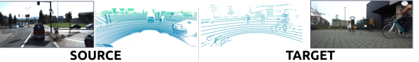
Figure 1: Comparison of KITTI (source) and robot data (target). We observe that differences in operating environments, sensor positions, and LiDAR density create a large domain gap. This presents a significant challenge for LiDAR-based 3D object detectors, as well as for the task of domain adaptation.

In this study, we address UDA in scenarios involving sparse LiDAR and large domain shifts: 1) between widely used automotive datasets, 2) for sim-to-real tasks and 3) for larger domain shifts using the last-mile delivery robot with a 16-layer LiDAR sensor operating on a sidewalk and indoors.

Inspired by 2D image-based adversarial DA [8, 3, 65], we propose a novel approach for 3D point cloud data: Unsupervised Adversarial Domain Adaptation for 3D Object Detection (UADA3D). Our method uses adversarial adaptation based on class-wise domain discriminators with a gradient reversal layer (GRL) to facilitate the learning of domain-invariant representations. The domain discriminator is trained to maximize its ability to distinguish between the target and source domains, while the model is trained to minimize this ability, resulting in domain-invariant feature learning.

The approach we present offers significant advantages over existing UDA methods for LiDAR-based 3D object detection: UADA3D does not require pre-trained source models, avoids the complexity of teacher-student architectures, and eliminates the inherent uncertainties of pseudo-labels. Instead, it directly learns features that are invariant across the source and target domains. Furthermore, our approach successfully adapts models to multiple object classes simultaneously (e.g. vehicle, pedestrian, and cyclist classes), a capability not often achieved by other SOTA methods. Importantly, this approach is particularly well-suited for applications with larger domain shifts such as multiple object categories, dissimilar operation environments, and sparse LiDAR data.

Our main contributions are as follows: (i) we highlight the limitations of existing UDA methods in considering substantial domain shifts beyond the typical domain variations associated with classical self-driving car applications (Section 2); (ii) we introduce UADA3D, an unsupervised adversarial domain adaptation approach for 3D LiDAR-based object detection (Section 3); (iii) we test UADA3D with two widely used object detection models and achieve SOTA performance in various challenging UDA scenarios (Section 4 and Section 5).

2 Related Work

LiDAR-based 3D Object Detection: The field of 3D object detection has evolved significantly over the years, with approaches for images [16, 47], point clouds [37, 60, 61, 10, 66, 57, 67] and multi-modal fusion [31, 1, 25, 28] proposed recently. PointNet [33] proposes an input invariant way or extracting features from point sets. Voxelnet [67] and PointPillars [20] propose partitioning the point clouds into a 3D voxel grid and pillars, respectively. Recently developed Centerpoint [63] combines voxel or pillar backbones with a center-based detection head. IA-SSD [66] proposes a single-stage point-based 3D detector that performs on par with other, much slower methods.

Unsupervised Domain Adaptation for LiDAR-based 3D Object Detection: Numerous research projects have focused on adapting 3D object detection models between high-resolution LiDAR datasets, ranging from 128 to 32 layers, typically found in self-driving scenarios [48, 56, 58, 59, 35, 43, 50, 32, 19, 42, 24, 64, 15]. However, little attention has been given to adapting these models to sparser LiDAR setups, which are common in small robotic platforms [38]. Notably, Peng et al.[32] and Wang et al.[49] focus specifically on model adaptation between LiDARs with 64 layers and 32 layers, and vice versa. Their results indicate that performance drastically decreases when models trained on 64-layer LiDAR data are adapted to a sparser 32-layer target domain. A similar pattern is observed in ST3D++[59], which leverages pseudo-labeling to generate labels for the target domain. MS3D++ [42] leverages multiple pre-trained detectors to achieve more accurate predictions, but again does not focus on very sparse data. Additionally, Cheng et al.[4] shown that very few UDA methods maintain consistent performance across different object classes, and the majority of the methods adapt only between the Car/Vehicle class, however, they do not focus on sparse LiDAR or different operating environments.

Recent works, such as DTS [14], which uses a student-teacher architecture with feature-level graph matching, show performance degradation with 16-layer LiDAR, although they do not report quantitative results. LiDAR Distillation (L.D.) [51] focuses exclusively on adapting models to sparser domains by using regression loss to minimize the difference between the BEV-feature maps predicted by student and teacher networks. However, their evaluations are conducted solely on autonomous driving datasets. While they extensively discuss the use of artificially downsampled 16-layer LiDAR data, they do not consider factors such as LiDAR sensor position (e.g., large height shift), domains that differ significantly (e.g., sidewalks versus from the street), nor multiple classes.

Most of the methods discussed above rely on a student-teacher approach, meaning they require a model pre-trained on the source domain to distill knowledge from the teacher to the student and/or to generate pseudo labels. In contrast, our method employs an adversarial learning approach. Consequently, we do not depend on a pre-trained teacher model to generate, for example, pseudo labels, which are not necessarily high-quality substitutes for ground truth and may even result in decreased model performance, as we later demonstrate in Section 5.

Adversarial Domain Adaptation: Adversarial domain adaptation (ADA) relies on a discriminative network structure that leverages domain discriminators to achieve domain invariance [13, 23, 27, 65, 45]. The GRL [8] reverses gradients linking the feature extractor and the discriminator. This end-to-end training simultaneously employs source and target data, aligning features across domains while minimizing detection loss in the source data. Following this, Chen et al.[3] introduced a two-stage adaptation method, incorporating image-level and instance-level adaptation. Saito et al.[34] proposed strong and weak adaptation, emphasizing local object feature alignment. He and Zhang [11] employed multiple GRLs for global adaptation at different convolutional layers. Xu et al.[55] introduced categorical regularization between image- and instance-level domain classification, using a regularization loss based on Euclidean distance. Li et al.[22] introduced AdvGRL, replacing the constant hyperparameter $\lambda$ with an adaptive $\lambda_{adv}$ to address challenging training samples. ADA has found a lot of use in object detection, classification, or segmentation in image space [3, 8, 65, 46, 27, 17].

In our work, we concentrate on adversarial domain adaptation in LiDAR-based 3D object detection, distinct from 2D methods. Our approach tackles the unique challenges of spatial data handling, arising from different point cloud densities and operating environments, through data augmentation and method design. We address it particularly with our discriminator utilizing features masked by 3D bounding boxes. Extracting these features from sparser, irregularly spaced point clouds is significantly more challenging than from pixel grids. This often requires transitioning to representations like Bird-Eye-View (BEV) feature space, as illustrated in Fig. 4. Additionally, working with point clouds involves making predictions based on partially missing, occluded, or incomplete data (as we can observe in qualitative results in supplementary materials), caused by low angular resolution, potentially resulting in a small number of points per object, even at short distances to the object. In the realm of UDA for segmentation, existing methods employ adversarial approaches with marginal alignment or non-adversarial methods [62, 46, 17, 26, 7]. Our approach utilizes conditional alignment, which we found to yield superior performance for LiDAR-based 3D object detection (see Section 5.1 for a comparison).

3 Method

3.1 Problem Formulation

Suppose that $Q$ is a point cloud, and $X$ is its feature representation learned by the feature extraction network $f_{\theta_{f}}$. The detection head $h_{\theta_{y}}$ uses these features to predict $P(Y|X)$, where $Y=(y,b)$ are the category labels $y$ and bounding boxes $b$. $Q$ is sampled from the source domain $\mathcal{D}_{s}$ and target domain $\mathcal{D}_{t}$. The objective is to learn a generalized $\theta_{f}$ and $\theta_{y}$ between domains such that $P(Y_{s},X_{s})\approx P(Y_{t},X_{t})$. Since $P(Y,X)=P(Y|X)P(X)$, the domain adaptation task for LiDAR-based object detectors is to align the marginal probability distributions $P(X_{s})$ and $P(X_{t})$ as well as the conditional probability distributions $P(Y_{s}|X_{s})$ and $P(Y_{t}|X_{t})$. Note that target labels $Y_{t}$ are not available during training, thus we must use unsupervised domain adaptation.

3.2 Method Overview

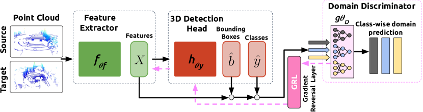
Figure 2: An overview of UADA3D (black arrows show forwards, and pink backwards pass). While the primary task of $f_{\theta_{f}}$ and $h_{\theta_{y}}$ is 3D object detection, the discriminator $g_{\theta_{D}}$ aims to classify the domain of each detected instance. Discriminator’s loss, reversed by GRL, encourages the detector to learn features that are not only effective for object detection but also invariant across domains.

Marginal adaptation, i.e., aligning $P(X)$, overlooks category and position labels, which can lead to uneven and biased adaptation. This may reduce the target domain’s discriminative ability. Aligning $P(Y|X)$ places direct emphasis on the task-specific outcomes (class labels and bounding boxes) in relation to the features. By focusing on $P(Y|X)$, we hypothesize that the adaptation process also becomes more robust to variations in feature distributions across domains, concentrating on the essential task of detecting objects. Furthermore, in Fig. 4, we show that the distribution of points in different categories per object varies significantly between the datasets due to LiDAR density, position and operating environment, while the vehicle size slightly varies, depending on the dataset country of origin (see Figs. 5(a), 5(b) and 5(c)). While we chose to use conditional alignment, we compare our method with different alignment strategies: marginal and joint distribution alignment in Section 5.1.

Fig. 2 provides a schematic overview of our method UADA3D. In each iteration, a batch of samples $Q$ from source $\mathcal{D}_{s}$ and target $\mathcal{D}_{t}$ domain is fed to the feature extractor $f_{\theta_{f}}$. Next, for each sample, features are extracted, and fed to the detection head $h_{\theta_{y}}$ that predicts 3D bounding boxes (lines 3-4 in LABEL:alg:UDA). The object detection loss (described in supplementary materials) is calculated only for the labeled samples from source domain (lines 6-7). The probability distribution alignment branch uses the domain discriminator $g_{\theta_{D}}$ (line 9) to predict from which domain samples came from, based on the extracted features $X$ and predicted labels $\hat{Y}$. The domain loss $\mathcal{L_{C}}$ is calculated for all samples (line 9). Next, the $\mathcal{L_{C}}$ is backpropagated through the discriminators (line 10), and through the gradient reversal layer (GRL) with the coefficient $\lambda$, that reverses the gradient during backpropagation, to detection head and feature extractor (lines 11-12). This adversarial training scheme works towards creating domain invariant features. Thus, our network learns how to extract features that will be domain invariant but also how to provide accurate predictions. Therefore, we seek for the optimal parameters $\theta_{f}^{*}$,$\theta_{y}^{*}$, and $\theta_{D}^{*}$, that satisfy:

$$\begin{array}[]{cc}\theta_{D}^{*}=\arg\!\min\limits_{\theta_{D}}\mathcal{L}_{C}\\ (\theta_{f}^{*},\theta_{y}^{*})=\arg\!\min\limits_{\theta_{f},\theta_{y}}\mathcal{L}_{det}-\lambda\mathcal{L}_{C}|_{\theta_{D}^{*}}\end{array}$$ (1)

where $\mathcal{L}_{det}$ is the detection loss (described in supplementary materials) calculated only for the labeled source domain, $\mathcal{L}_{C}$ is the domain loss calculated for both source and target domains. $\lambda=0.1$ is the GRL coefficient, which is discussed further in Section 5.1.

3.3 Feature Masking

Feature masking plays a crucial role in predicting the domain based on specific object features. Masking enables the model to focus solely on the features corresponding to each instance, thus enhancing the relevance and accuracy of the domain prediction. In Fig. 4, we show how features extracted from a point cloud $Q$ are masked and used for domain prediction. The input to the class-wise domain discriminators $g_{\theta_{D,k}}$ is $(x,\hat{b})$, where $x$ are masked features, $\hat{b}$ are predcited bounding boxes, and $(a,b)$ denotes a concatenation. To obtain masked features $x$, we mask the feature map $X=f_{\theta f}(Q)$ with each predicted bounding box $\hat{b}_{n}$ creating corresponding masked features $x_{n}$. Finally, we concatenate $x_{n}$ with the bounding box $\hat{b}_{n}$ and feed to the corresponding class-wise discriminator $g_{\theta_{D,k}}$.

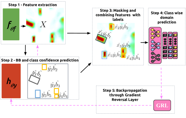
Figure 3: Flowchart showing feature masking and domain prediction in UADA3D.

[width=]figures/bar_plots/pts_cls

Figure 4: Average number of points in an object per class.

3.4 Conditional Distribution Alignment

The conditional distribution alignment module shown in Figs. 2 and 4, has the task of reducing the discrepancy between the conditional distribution $P(Y_{s}|X_{s})$ of the source and $P(Y_{t}|X_{t})$ of the target. As we highlighted in Section 3.2, shown in Fig. 4 and later discussed in Section 4.1, we can see a large difference between how objects from each category appear in different domains. Thus, instead of having one discriminator, we use $K=3$ class-wise domain discriminators $g_{\theta_{D},k}$, corresponding to vehicle, pedestrian, and cyclist classes. The conditional distribution alignment module is trained using the least-squares loss function:

$$\mathcal{L}_{C}=\frac{1}{N}\sum_{n=1}^{N}\hat{y}_{k,n}\odot(g_{\theta_{D},k}(x_{n},\hat{b}_{n})-d)^{2}$$ (2)

where $N$ is the number of labels, $\hat{y}_{k,n}$ corresponding class confidence of instance $n$ and $\odot$ is element-wise multiplication. The loss is backpropagated to the discriminators (line 9 in LABEL:alg:UDA). Next, $\mathcal{L}_{C}$ is backpropagated through GRL to the detection head $h_{\theta_{y}}$ and the feature extractor $f_{\theta_{f}}$.

3.5 Data Augmentation

Differences between LiDAR domains include different densities and object sizes. We use downsampling, a commonly used augmentation approach since the domain gap can be partially remedied by reducing LiDAR layers of the source data to $16$ or $32$ to better match the target domain LiDAR data as highlighted in [53, 6]. LiDAR-CS [6], Waymo [39], and nuScenes [2] datasets contain vehicle sizes that correspond to the large vehicle sizes found in the USA, while our robot and KITTI [9] are collected in Europe where vehicles are generally smaller. Random object scaling (ROS) [59] is applied in the source domain to address this vehicle size bias. While previous UDA methods on LiDAR-based 3D object detection often apply domain adaptation only to a single object category, we consider it a multiclass problem. Thus, we chose ROS with different scaling intervals for the three classes, described in detail in supplementary materials.

4 Experiments Setup

[width=]figures/bar_plots/size_CS

(a) Vehicle size LiDAR-CS

[width=]figures/bar_plots/size_kitti

(b) Vehicle size KITTI

[width=]figures/bar_plots/size_Laura

(c) Vehicle size robot data

[width=]figures/bar_plots/number_CS

(d) Distance to objects LiDAR-CS

[width=]figures/bar_plots/number_kitti

(e) Distance to objects KITTI

[width=]figures/bar_plots/number_Laura

(f) Distance to objects robot data

Figure 5: Comparison of objects in LiDAR-CS, KITTI and robot datasets.

We compare performance of IA-SSD [66] and Centerpoint [63] on large number of UDA scenarios using our method, UADA3D, against that of other SOTA unsupervised domain adaptation approaches (ST3D++ [59], DTS [14], L.D. [51], and MS3D++ [42]). In IA-SSD, the adaptive discriminator network is made of fully-connected layers that operate on down-sampled point features. In Centerpoint, the discriminator makes use of 2D convolutions with inputs from Bird’s Eye View (BEV) feature maps. The most prominent distinction between the two networks is the point-based and view-based representations, which are handled by MLPs and 2D convolutions respectively. The ability to adapt both of these models between the domains shows the modularity of our solution and adaptivity to different methods. With UADA3D, Centerpoint is trained for 40 and IA-SSD for 80 epochs using one-cycle Adam [18] with a learning rate 0.003 and 0.01 respectively. The GRL-coefficient was set to a fixed value of 0.1. For all the SOTA methods, we train the source-only and oracle models with 40 (Centerpoint) and 80 (IA-SSD) epochs, then we adapt them for 40. Detailed information on source model training and hyperparameters is provided in supplementary materials.

4.1 Datasets

We use five datasets: LiDAR-CS [6] that provide multiple LiDAR resolutions (we use VLD-64 “CS64”, VLD-32 “CS32”, and VLP-16 “CS16”), KITTI [9] “K” (with HDL-64E), Waymo [39] “W” (HDL-64E), nuScenes [2] “N” (VLD-32) and data collected with the last mile delivery robot “R” (with VLP-16) in different locations in Europe, further described in supplementary materials.

First, we focus on UDA between autonomous driving datasets, from denser to sparser LiDARs, since this is where the other SOTA methods perform the worst. Even though these sensors operate similarly, differences arise from the point-cloud density as well as LiDARs azimuth and elevation angles. Second, we adapt to our robot data, which is particularly challenging due to different LiDAR positions and densities on the mobile robot, as well as the operating environment (sidewalk vs. street). Finally, we compare the performance of adaptation from sparser to denser domains between autonomous driving datasets.

In Fig. 5 we can see how big the gap between the self-driving datasets and robot data is, especially in distance to the objects (nuScenes and Waymo show similar distribution to LiDAR-CS and KITTI). The distance to the objects encountered in the robot data, seen in Figure 5(f), shows that the dataset only contains objects closer than $15$m, with a majority of pedestrians and cyclists closer than $10$m and all vehicles in the $10-15$m range, since the robot drives on a sidewalk. In contrast, in the self-driving cars dataset Fig. 5(d) and Fig. 5(e), a lot of objects are between $20-30$m away. Consequently, the average number of points per object (Fig. 4), is very different between the datasets. This is causing the instances to significantly differ between these domains. While the different vehicle sizes are often addressed in 3D domain adaptation approaches [59], to the best of our knowledge, differing number of points per object has not been examined by other UDA works before.

KITTI dataset is limited by having labels only in the front camera field of view (FOV), while other datasets feature labels in a 360-degree FOV. This presents a significant challenge for domain adaptation, typically leading researchers to adapt to the KITTI datasets, rather than from them, and when they do, it results in marginal improvements or even a decrease in performance [51].

4.2 Evaluation metrics

We report $mAP_{3D}$ and $mAP_{BEV}$, closed gap and change in $mAP$. $mAP$ is the mean average precision over the three classes: Vehicle, Pedestrian, and Cyclist. Closed gap [61] is calculated as $\frac{mAP_{model}-mAP_{source}}{mAP_{oracle}-mAP_{source}}\times 100\%$ and tells how close we are to a model trained on the target domain (oracle).

5 Results

Table 1: Comparison of performance of different adaptation methods on source to target (S$\rightarrow$T) domain adaptation tasks. We report $mAP_{3D}$ and $mAP_{BEV}$over Vehicle, Pedestrian and Cyclist. The best score is bold and the second best is underline.

		Models
		IA-SSD [66]			Centerpoint [63]
S→T	Methods	3D/BEV	Change	Closed Gap	3D/BEV	Change	Closed Gap
	Source Only	24.57 / 35.82	-/-	-/-	34.92 / 47.25	-/-	-/-
	ST3D++ [59] (TPAMI’22)	36.61/41.56	12.05/ 5.74	69.77% / 46.60%	50.17 / 55.74	17.59/ 8.49	78.52 % / 51.83 %
	DTS [14] (CVPR’23)	31.54 / 36.96	6.97/ 1.14	40.39 %/ 9.26 %	48.32 / 55.02	15.74/ 7.78	68.99 % / 47.44 %
CS64	L.D. [51] (ECCV’22)	29.85 / 38.50	5.29 / 2.68	30.62 % / 21.74 %	50.91/58.37	15.99 / 11.12	82.31 % / 67.83 %
→	MS3D++ [42](ITSC’23)	30.74 / 31.00	6.18 / -4.85	23.01% / -39.18 %	40.09 / 42.79	5.17 / -4.45	26.26 % / -27.17 %
CS32	UADA3D (ours)	37.25/ 45.75	12.68 / 9.92	73.44 % / 80.61 %	54.02/ 60.77	19.11/ 13.52	98.34 % / 82.47 %
	Oracle	41.83 / 48.13	-/-	-/-	54.35 / 63.64	-/-	-/-
	Source Only	$\times$	$\times$	$\times$	25.22 / 33.93	-/-	-/-
	ST3D++ [59]	$\times$	$\times$	$\times$	17.71 / 18.02	-7.51 / -15.91	-25.78 % / -53.55 %
	DTS [14]	$\times$	$\times$	$\times$	18.05 / 19.77	-7.17 / -14.16	-24.62 % / -47.66 %
K	L.D. [51]	$\times$	$\times$	$\times$	27.35/35.20	2.13 / 1.27	7.31 % / 4.27 %
→	MS3D++ [42]	$\times$	$\times$	$\times$	30.34/ 35.26	5.12 / 1.33	17.58 % / 4.48 %
CS32*	UADA3D (ours)	$\times$	$\times$	$\times$	32.49/34.79	7.27/ 0.86	24.96 % / 2.89 %
	Oracle	$\times$	$\times$	$\times$	54.35 / 63.64	-/-	-/-
	Source Only	1.5 / 4.5	-/-	-/-	15.96 / 17.87	-/-	-/-
	ST3D++ [59]	11.94 / 13.15	10.45 / 8.65	23.38 % / 20.09 %	17.66 / 22.83	1.71 / 4.97	4.6 % / 13.45 %
	DTS [14]	15.82 / 17.40	14.32 / 12.90	32.03 % / 29.97 %	16.24 / 17.89	0.28 / 0.02	0.78 % / 0.05 %
W	L.D. [51]	17.57 / 19.33	16.07 / 14.83	35.95 % / 34.46 %	22.21 / 27.98	6.26 / 10.12	16.96 % / 27.41 %
→	MS3D++ [42]	15.10 / 16.61	13.60 / 12.11	30.43 % / 28.15 %	19.71/ 21.69	3.75 / 3.82	10.17 % / 10.35 %
N	UADA3D (ours)	18.33 / 18.55	16.83 / 14.05	37.66 % / 32.66 %	26.89 / 30.67	10.94 / 12.80	29.65 % / 34.68 %
	Oracle	46.20 / 47.53	-/-	-/-	52.84 / 54.77	-/-	-/-
	Source Only	20.11 / 25.26	-/-	-/-	22.33 / 38.08	-/-	-/-
	ST3D++ [59]	30.11 / 40.09	10.00 / 14.83	36.09 % / 48.63	43.90/50.42	21.57 / 12.34	73.99 % / 57.40 %
	DTS [14]	33.41/42.62	13.29 / 17.36	47.98 % / 56.92 %	39.19 / 47.81	16.86 / 9.73	57.86 % / 45.26 %
CS64	L.D. [51]	29.81 / 35.35	9.70 / 10.10	34.99 % / 33.11 %	42.66/ 54.07	20.33 / 15.99	69.76 % / 74.38 %
→	MS3D++ [42]	32.79 / 37.21	12.68 / 11.95	45.77 % / 39.17 %	30.98 / 38.53	8.65 / 0.45	29.68 % / 2.08 %
CS16	UADA3D (ours)	35.32/ 45.53	15.21 / 20.27	54.87 % / 66.47 %	43.59 / 52.93	21.26/ 14.85	72.94% / 69.04%
	Oracle	47.82 / 55.76	-/-	-/-	51.48 / 59.58	-/-	-/-
	Source Only	38.73 / 43.94	-/-	-/-	41.49 / 52.15	-/-	-/-
	ST3D++ [59]	39.75 / 44.47	1.02 / 0.53	11.19 % / 4.49 %	44.01 / 52.60	2.51 / 0.45	25.14 % / 6.05 %
	DTS [14]	40.27 / 43.95	1.55 / 0.01	16.76 % / 0.11 %	42.29 / 52.26	0.80 / 0.11	8.01 % / 1.48 %
CS32	L.D. [51]	38.99 / 44.24	0.26 / 0.30	2.82 % / 2.54 %	43.34 / 52.92	1.84 / 0.77	18.46 % / 10.34 %
→	MS3D++ [42]	40.25 / 44.38	1.52 / 0.44	16.73 % / 3.72 %	41.16 / 49.27	0.12 / -2.88	1.17 % / -38.79
CS16	UADA3D (ours)	41.71/ 48.51	2.97 / 4.57	32.72 % / 38.69 %	44.35/ 53.25	2.86 / 1.10	28.64 % / 14.75 %
	Oracle	47.82 / 55.76	-/-	-/-	49.14 / 59.58	-/-	-/-
	Source Only	7.28 / 12.93	-/-	-/-	5.38 / 25.97	-/-	-/-
	ST3D++ [59]	31.79 / 42.19	24.50 / 29.26	66.53 % / 74.69 %	23.30 / 33.99	17.92 / 8.01	41.67 % / 23.88 %
CS64	DTS [14]	33.68 / 46.19	26.40 / 33.26	71.69 % / 84.90 %	16.87 / 32.13	11.50 / 6.16	26.73 % / 18.34 %
→	L.D. [51]	20.70 / 32.10	13.41 / 19.17	36.42 % / 48.94 %	28.13 / 38.90	22.75 / 12.93	52.89 % / 38.51 %
R	MS3D++ [42]	$\times$	$\times$	$\times$	14.44 / 37.88	9.06 / 11.90	21.06 % / 35.47 %
	UADA3D (ours)	33.00 / 43.02	25.72 / 30.09	69.83 % / 76.81 %	28.87 / 40.09	23.49 / 14.12	54.62 % / 42.07 %
	Source Only	$\times$	$\times$	$\times$	24.40 / 33.81	-/-	-/-
	ST3D++ [59]	$\times$	$\times$	$\times$	31.57 / 35.51	7.17 / 1.70	16.19 % / 4.58 %
K	DTS [14]	$\times$	$\times$	$\times$	23.24 / 23.56	-1.16 / -10.25	-2.63 % / -27.69 %
→	L.D. [51]	$\times$	$\times$	$\times$	39.46 / 41.47	15.06 / 7.66	33.98 % / 20.71 %
R	MS3D++ [42]	$\times$	$\times$	$\times$	21.58 / 25.72	-2.28 / -8.09	-6.36 % / -21.85 %
	UADA3D (ours)	$\times$	$\times$	$\times$	40.08 / 41.78	16.40 / 7.97	37.01 % / 21.54 %
	Source Only	8.33 / 15.93	-/-	-/-	3.78 / 6.00	-/-	-/-
	ST3D++ [59]	21.57 / 31.04	13.25 / 15.11	37.02 % / 41.77 %	26.57 / 40.68	22.80 / 34.69	51.09 % / 64.79 %
CS32	DTS [14]	15.37 / 26.94	7.05 / 11.01	19.69 % / 30.45 %	18.68 / 29.65	14.91 / 23.65	33.41 % / 44.18 %
→	L.D. [51]	19.43 / 31.38	11.10 / 15.45	31.02 % / 42.70 %	26.89 / 36.85	23.12 / 30.85	51.82 % / 57.62 %
R	MS3D++ [42]	$\times$	$\times$	$\times$	4.45 / 42.46	0.68 / 36.46	1.52 % / 68.09 %
	UADA3D (ours)	22.15/ 31.90	13.82 / 15.97	38.62 % / 44.14 %	31.54/ 42.82	27.76 / 36.83	62.23 % / 68.78 %
	Source Only	10.28 / 15.26	-/-	-/-	15.07 / 33.97	-/-	-/-
	ST3D++ [59]	9.58 / 29.83	-0.7 / 14.56	-2.07 % / 39.53 %	33.22 / 42.62	18.15 / 8.65	54.46 % / 33.84 %
CS16	DTS [14]	11.95 / 27.59	1.67 / 12.32	4.93 % / 33.45 %	17.35 / 34.34	2.28 / 0.37	6.84 % / 1.45 %
→	L.D. [51]	9.48 / 23.27	-0.81 / 8.01	-2.38 % / 33.45 %	27.13 / 40.19	12.06 / 6.22	36.19 % / 24.32 %
R	MS3D++ [42]	$\times$	$\times$	$\times$	2.16 / 32.30	-12.91 / -1.67	-38.75 % / -6.52 %
	UADA3D (ours)	19.71 / 35.69	19.71 / 20.42	27.87 % / 55.44 %	41.47 / 46.86	26.40 / 12.89	79.24 % / 50.43 %
Robot	Oracle (R)	44.11 / 52.10	-/-	-/-	48.39 / 59.54	-/-	-/-

• In all the adaptation scenarios, we analyze three classes: Vehicles, Pedestrians, and Cyclists. However, in the case of K →CS32, we focus solely on the Vehicle class, as the adaptation attempts for the other classes were unsuccessful for all the methods.

• These scenarios were not tested.

Table 2: Comparison of performance of different adaptation scenario on sparse to dense task. $mAP_{3D/BEV}$ reported over 3 classes: Vehicle, Pedestrian, and Cyclist.

	CS16 →CS64 (IA-SSD [66])		CS16 →CS64 (Centerpoint [63])		N →W (Centerpoint [63])		N →K (Centerpoint [63])
	3D/BEV	Closed Gap	3D/BEV	Closed Gap	3D/BEV	Closed Gap	3D/BEV	Closed Gap
Source	18.8/22.17	-/-	25.92/33.62	-/-	19.61/37.76	-/-	17.18/40.18	-/-
ST3D++	41.32/46.96	42.12%/ 47.59%	19.22/19.90	34.79%/ 40.57%	29.37/40.07	26.32%/ 10.89%	20.37/44.02	11.66%/36.99%
DTS	45.56/51.91	50.06%/57.09%	56.68/64.87	55.66%/63.71%	32.33/41.10	34.31%/15.77%	18.90/46.20	6.30%/57.95%
MS3D++	38.61/42.34	37.06%/ 38.73%	51.12/55.60	45.58%/ 44.79%	21.82/39.92	5.97%/10.19%	18.00/40.61	2.98%/4.41%
UADA3D	50.96/53.63	60.15%/ 60.41%	51.87/59.40	46.95%/ 52.56%	35.68/42.78	43.33%/23.72%	21.97/48.52	17.51%/80.35%
Oracle	72.26/74.25	-/-	81.17/82.68	-/-	56.69/58.96	-/-	44.51/50.56	-/-

[trim=1.8cm 0cm 0cm 0,clip,width=]figures/bar_plots/bars_classes

Figure 6: Per class $AP_{3D}$ in adaptation experiments on IA-SSD (left) and CenterPoint (right). Vehicle, Pedestrian, and Cyclist. UADA3D is our method.

In Table 1 and Table 2, we compare our method with SOTA on a large number of adaptation scenarios between source and target (S $\rightarrow$ T) data (further tests are included in supplementary materials). In Table 1 we focus on 9 different dense to sparse scenarios for the two models: Centerpoint [63] and IA-SSD [66]. Our method, UADA3D, outperforms other SOTA approaches in most cases achieving much higher improvements, especially when it comes to the larger domain gaps (adapting models towards mobile R(obot) or W$\rightarrow$ N). By analyzing Change and Closed Gap columns, we can observe that Centerpoint often shows higher adaptability and substantially higher improvement $mAP_{3D}$ and $mAP_{BEV}$ than IA-SSD. That may come from the fact that for IA-SSD, we have to fix a specific number of sampling points (explained in supplementary material), which makes the model less flexible when adapting across different LiDAR densities and patterns. Furthermore, even though other SOTA methods may outperform UADA3D on individual classes (only Cyclist in adaptation towards R), they perform worse in others categories (Fig. 6). This demonstrates that UADA3D offers better generalization across different detectors and classes.

We observe that our method handles diverse domain shifts effectively when adapting between autonomous driving datasets (Waymo, KITTI, nuScenes), simulation data (LiDAR-CS), and robot data (R). As mentioned in Section 3, UADA3D does not need a pre-trained teacher model, as all the other approaches do. Instead, we can directly train the domain-adapted model, leveraging the GRL functionality which creates domain-invariant features. This allows our method to successfully train high-performing models on unlabeled target data, without depending on pseudo labels. We can observe in Table 1 that some of the methods perform even worse than the source-only approaches when tested on adaptation towards more challenging scenarios (e.g K $\rightarrow$ R), failing to generate accurate pseudo labels or distill teacher knowledge. Additionally, it is important to note that UADA3D never achieves lower performance than source-only models, on the adaptation task, regardless if the domain gap is big (e.g., K$\rightarrow$ R, W $\rightarrow$ N) or small (e.g., CS32 $\rightarrow$ CS16). Notably, K$\rightarrow$R or CS16$\rightarrow$R adaptations appear particularly difficult, as many methods perform worse than source-only, suggesting that adapting to the robot’s environment poses distinct challenges. However, despite this, the gap in those cases seems easier to close than the domain gap between W $\rightarrow$ N or K$\rightarrow$CS32, where the improvement and the closed gap were the lowest. That may be caused by the large dataset range and scale in the former, and the limited FOV of KITTI, in the latter.

In Table 2, we compare methods’ performance on sparse to dense cases. UADA3D performs best in 3 out of 4 tasks and second best in one, consistent with the dense to sparse results. All methods excel when adapting from sparse to dense data, indicating that target data is richer in information, compared to the source. This supports our hypothesis that adapting from dense to sparse is more challenging. Our method performs well on both: sparse to dense and dense to sparse, while some SOTA methods, like L.D. [51], only allow adaptation from dense to sparse LiDAR, highlighting our method’s generalizability.

5.1 Ablation Studies

We explore the impact of various factors on our method’s performance. First, we ask the question of which probability distribution alignment is the most beneficial for UADA3D. Next, we investigate the impact of discriminator design and analyze GRL parameters. Finally, we integrate other self-learning components to enhance our method further. Further details, including ablations and hyperparameter studies, can be found in the supplementary materials.

Probability Distribution Alignments: In these ablation studies, we explore the effectiveness of other probability distribution alignment strategies, shown in Fig. 7. In UADA3D with the marginal distribution alignment, UADA3D_{$\mathcal{L}m$}, the discriminator gradient is backpropagated only to the feature extractor with loss $\mathcal{L}_{m}$, where $\mathcal{L}_{m}=\frac{1}{N}\sum_{n=1}^{N}d\cdot\log(g_{\theta_{m}}(X_{n}))+(1-d)\cdot\log(1-g_{\theta_{m}}(X_{n}))$, where $d$ is 0 for source and 1 for target domains and $g_{\theta_{M}}$ denotes the marginal discriminator network. In UADA3D (i.e., UADA3D_{$\mathcal{L}c$}) the discriminator gradient is backpropagated to the detection head through the whole model. UADA3D_{$\mathcal{L}mc$} combines marginal and conditional alignment with $\mathcal{L}_{mc}=(\mathcal{L}_{m}+\mathcal{L}_{C})$, where $\mathcal{L}_{C}$ is given in Eq. 2. UADA3D_{$\mathcal{L}m$} uses feature maps directly to predict the domain and calculate the loss, while UADA3D employs masked features with class labels and bounding boxes. Conditional probability distribution alignment consistently yields high-quality outcomes, but there are cases where it is not the best one. UADA3D_{$\mathcal{L}m$} delivers comparable results, especially in cross-sensor adaptation for self-driving cars, due to significant differences in the marginal probability distribution $P(X)$. While UADA3D_{$\mathcal{L}m$} and UADA3D_{$\mathcal{L}mc$} sometimes outperform UADA3D, they underperform in some scenarios such as IA-SSD adaptation to R. Consequently, we selected conditional alignment as our preferred method.

[trim=1cm 0cm 0cm 0,clip,width=]figures/bar_plots/ablation_UADA

Figure 7: Comparison UADA3D performance with different probability distribution alignments on IA-SSD (left) and CenterPoint (right).

Discriminator designs: In Table 3 we examine different discriminator designs: (a) single domain discriminator with the input of $(x_{n},\hat{b}_{n})$, without any label information, (b) a single domain discriminator where the output is multiplied with the maximum predicted class confidence $\hat{y}_{max,n}\odot g_{\theta_{D}}(x_{n},\hat{b}_{n})$, and (c) the default UADA3D setting with three domain discriminators. (a) and (b) obtain higher adaptation scores in some cases, especially on Centerpoint CS64$\rightarrow$R, but worse than (c) on IA-SSD. When comparing (a) and (b), we can see that the multiplication with $\hat{y}_{max}$ (b) has quite some impact. Centerpoint obtains better performance using one discriminator than IA-SSD, which is likely due to the easier transferability of BEV features compared to point features. This is also seen in the $AP_{BEV}$ scores of IA-SSD that improve more than the $AP_{3D}$ for cases (a) and (b). Due to higher model complexity, IA-SSD appears to gain the most advantage from the use of multiple class-wise conditional discriminators (c). While IA-SSD performs the best with (c) and Centerpoint with (b), to be consistent, we chose option (c) as a default option for our method.

Table 3: Contribution of class-confidence and multiple discriminators ($AP_{3D}/AP_{BEV}$). $N_{D}$ is a number of class-wise discriminators, and $y$ denotes if we use class labels.

				CS64 →CS16			CS64 →robot
	Method	ND	y	V3D/BEV	P3D/BEV	C3D/BEV	V3D/BEV	P3D/BEV	C3D/BEV
IA [66]	source			29.97 / 38.10	11.02 / 14.62	19.35 / 23.05	1.17 / 5.77	6.42 / 18.10	14.26 / 14.92
	(a)	1		42.55 / 61.42	17.36 / 32.85	35.29 / 39.14	52.20 / 59.60	8.28 / 20.65	15.47 / 23.37
	(b)	1	$\checkmark$	40.92 / 61.61	17.75 / 32.51	34.99 / 39.81	59.85 / 67.66	11.32 / 25.70	14.01 / 16.51
	(c)	3	$\checkmark$	42.96 / 62.08	25.08 / 34.09	37.91 / 40.42	53.29 / 63.93	14.20 / 28.58	31.51 / 36.55
Cent [63]	source			32.30 / 48.08	11.63 / 20.09	23.06 / 46.07	1.11 / 48.16	3.03 / 14.06	11.99 / 15.70
	(a)	1		47.95 / 65.84	39.21 / 49.00	45.91 / 47.38	46.94 / 54.89	25.04 / 44.12	39.43 / 44.57
	(b)	1	$\checkmark$	47.62 / 65.43	40.28 / 49.42	46.08 / 47.41	50.81 /58.72	27.68 / 45.39	47.88 / 51.56
	(c)	3	$\checkmark$	46.99 / 66.01	38.22 / 49.47	45.56 / 48.30	44.53 / 53.11	20.65 / 33.50	21.43 / 33.67

Gradient reversal coefficient: We tested two different strategies for GRL-coefficient $\lambda$ on UADA3D and UADA3D_{$\mathcal{L}m$}. Firstly, a constant $\lambda=0.1$ was tested following the setting used for most adversarial UDA strategies in 2D object detection [3, 34]. Secondly, we follow other approaches [8, 22] where $\lambda$ was increased over the training according to: $\lambda=\alpha(\frac{2}{1+exp(-\gamma p)}-1)$, where $\alpha\in[0,1]$ is a scaling factor that determines the final $\lambda$, $\gamma=10$ and $p$ is the training progress from start $0$ to finish $1$. $\alpha$-values of $1,0.5,0.2,0.1$ were tested. In this way, the gradient reversal is low for the first few iterations and goes towards $\alpha$. Given that we do not use a pre-trained model, this approach enables the method to concentrate on the object detection task at the beginning of training, as the discriminator loss will initially be significantly smaller. In Table 5, we can observe that smaller $\lambda$ values result in better adaptation performance. The best score for vehicles and cyclists was achieved with the constant $\lambda=0.1$ while the dynamic $\lambda$ achieved the best scores for pedestrians at $\alpha=0.1$ respectively. Both $\lambda=0.1$ and $\alpha=0.1$ yielded good average scores across all three classes with minimal differences. However, we opted for constant $\lambda=0.1$ in our experiments as it demonstrated slightly better performance and reduced the complexity.

Table 4: Different gradient reversal coefficients of IA-SSD, for CS64 $\rightarrow$ CS16.

$\lambda$	UADA3D$\mathcal{L}m$/UADA3D
	$AP_{3D,V}$	$AP_{3D,P}$	$AP_{3D,C}$
Source-Only	29.97	11.02	19.35
0.1	48.48/42.96	25.48/25.08	38.12/37.91
$0.1(\frac{2}{1+exp(-\gamma p)}-1)$	42.76/41.06	26.43/26.80	33.77/31.83
$0.2(\frac{2}{1+exp(-\gamma p)}-1)$	40.14/38.11	24.55/24.7	34.22/30.01
$0.5(\frac{2}{1+exp(-\gamma p)}-1)$	40.24/37.55	23.58/21.42	33.16/27.43
$\frac{2}{1+exp(-\gamma p)}-1$	41.65/40.09	23.68/22.58	31.72/29.39
Oracle	58.62	35.57	49.27

Table 5: UDA methods with UADA3D component on W$\rightarrow$N.

Method	mAP3D/BEV	Closed Gap
Source only	15.96/17.87	-/-
U	26.89/30.67	29.65/34.68%
U+PM	22.86/34.11	18.73/44.02%
U+PM+PSL	32.01/36.58	29.65/50.71%
U+PM+MK	31.36/36.09	41.76/49.37%
U+PM+ME	28.94/35.63	35.19/48.14%
Oracle	52.84/54.77	-/-

Integration of additional self-learning components: We wanted to see how other self-learning components can further improve UADA3D. We combined UADA3D (U) with a pre-trained source model (PM), pseudo-labeling (PSL) [59], model ensemble (ME) [42] and mimicking regions (MK) [51] in BEV space. In Table 5 we show the results of adapting Centerpoint [63] on the W$\rightarrow$N task. We can see that our method can further benefit from the additional self-learning component and further close the domain gap. We can see that PSL further improves our method the most, but using only PM can slightly decrease UADA3D performance. To add these approaches we needed pre-trained source models that UADA3D does not require. Thus, we leave adding these functionalities, without the need for a pre-trained model, for future work.

6 Conclusions and Limitations

In this paper, we introduce UADA3D, a novel approach tailored for challenging UDA scenarios, specifically addressing sparser LiDAR data and mobile robots. Through adversarial training using gradient reversal, UADA3D effectively navigates diverse environments, ensuring precise object detection and achieving state-of-the-art performance across various domain adaptation scenarios. This way, the large number of existing data sets in the field of autonomous driving can also be leveraged for mobile robotics. However, domain gaps persist, notably in scenarios such as W(aymo) → N(uScenes) or K(ITTI) → R(obot), where improvements are constrained. Future work could explore adapting between multimodal scenarios, such as camera and LiDAR, radar and LiDAR, or adding more self-training components.

sec0em1.7em subsec1.2em2.35em Supplementary Material ECCV 2024 #7127

Supplementary materials

Appendix 0.A Experimental setup

We ran the experiments on two desktop computers with Intel Core i7-12700KF (12 cores, 20 threads) 5.00 GHz CPU and a NVIDIA GeForce RTX 3090 (24 GB) GPU. We used a batch size of $8$. For UADA3D, this leads to $4$ labeled frames from the source data and $4$ unlabeled frames from the target data. In our implementation, we used the OpenPCDet library [40]. Our code will be publicly available soon. While it is hard to estimate exactly how many GPU hours were spent on this project including hyperparameter search, ablation study etc., we can estimate the number of hours necessary for obtaining the main results (Table 1 in main paper). Note that one IA-SSD epoch is needs less time than one Centerpoint epoch, since IA-SSD is a more efficient detector.

Appendix 0.B Implementation Details

0.B.1 Detailed implementation of UADA3D

The conditional module has the task of reducing the discrepancy between the conditional label distribution $P(Y_{s}|X_{s})$ of the source and $P(Y_{t}|X_{t})$ of the target. The label space $Y_{i}$ consists of class labels $y\in\mathbb{R}^{N\times K}$ and 3D bounding boxes $b_{i}\in\mathbb{R}^{7}$. The feature space $X$ consists of point features $F\in\mathbb{R}^{N\times C}$ (IA-SSD) or the $2$D BEV pseudo-image $I\in\mathbb{R}^{w\times h\times C}$ (Centerpoint). The domain discriminator $g_{\theta_{D}}$ in Centerpoint has $2$D convolutional layers of $264,256,128,1$ while IA-SSD uses an MLP with dimensions $519,512,256,128,1$. LeakyReLU is used for the activation functions with a sigmoid layer for the final domain prediction. A kernel size of $3$ was chosen for Centerpoint, based on experiments shown in 0.B.4. Note, that we do class-wise domain prediction, thus we have $K$ discriminators corresponding to the number of classes (in our case $K=3$, but it can be easily modified).

0.B.2 Detailed implementation of UADA3D_{$\mathcal{L}m$}

The primary role $UADA3D_{\mathcal{L}m}$ with the marginal feature discriminator is to minimize the discrepancy between the marginal feature distributions of the source, denoted as $P(X_{s})$, and the target, represented by $P(X_{t})$. Here, $X_{s}$ and $X_{t}$ symbolize the features extracted by the detection backbone from the two distinct domains. This approach ensures the extraction of domain invariant features. The loss function of $UADA3D_{\mathcal{L}m}$ marginal alignment module is defined through Binary Cross Entropy.

The output of the point-based detection backbone in IA-SSD [66] is given by $N$ point features with feature dimension $C$ and corresponding encodings. Point-wise discriminators can be utilized to identify the distribution these points are drawn from. The input to the proposed marginal discriminator $g_{\theta_{D}}$ is given by point-wise center features obtained through set abstraction and downsampling layers. The discriminator is made up of $5$ fully connected layers (512,256,128,64,32,1) that reduce the feature dimension from $C$ to $1$. LeakyReLU is used in the activation layers and a final sigmoid layer is used for domain prediction.

The backbone in Centerpoint [63] uses sparse convolutions to extract voxel-based features that are flattened into 2D BEV-features. Therefore, the input to the view-based marginal discriminator is given by a pseudo image of feature dimension $C$ with spatial dimensions $w$ and $h$ that define the 2D BEV-grid. Since 2D convolutions are more computationally demanding over the MLP on the heavily downsampled point cloud in IA-SSD, the 2D marginal discriminator uses a $3$-layered CNN that reduces the feature dimension from $C$ to $1$ (256,256,128,1), using a kernel size of $3$ and a stride of $1$. Same as in the point-wise case, the loss function of $UADA3D_{\mathcal{L}m}$ is defined through Cross Entropy.

0.B.3 Detectors’ loss functions

The loss of our model is defined as the loss of the network $L_{det}$ and the loss of the discriminators. While in the main paper we explained how the discriminator loss works, in this section we want to provide more insight into $L_{det}$ used in both of the models we tested. We follow the description provided by the authors of Centerpoint [63] and IA-SSD [66] and their source code we adopted in our experiment. For more details, please refer to the original papers.

Centerpoint [63]: At the initial stage, the detection head’s main function involves determining essential features at object centers. This process includes refining sub-voxel locations $o\in\mathbb{R}^{2}$, measuring the object’s height above ground $h_{g}\in\mathbb{R}$, evaluating 3D sizes $s\in\mathbb{R}^{3}$, and calculating yaw rotation angles using $(\sin(\alpha),\cos(\alpha))\in\mathbb{R}^{2}$. The sub-voxel refinement $o$ aims to reduce quantization errors caused by voxelization and backbone striding, while the height measurement $h_{g}$ ensures precise 3D positioning and restores elevation details omitted in map-view projections. Yaw orientation is assessed through continuous regression of its sine and cosine components. Together with the bounding box dimensions, these attributes provide a comprehensive 3D bounding box profile. Each feature is processed through its respective head. In the training phase, ground truth centers are used in supervised training using L1 regression loss, and size regression is performed logarithmically to better accommodate different box shapes. During inference, these features are extracted from the outputs of dense regression heads at the peak positions of each object.

In the second stage, class-agnostic confidence scores and box refinements are predicted. Authors use score target $I$ guided by the box’s 3D IoU with the corresponding ground truth bounding box:

$$I=\min(1,\max(0,2\times\text{IoU}_{t}-0.5))$$ (3)

where $\text{IoU}_{t}$ is the IoU between the $t$-th proposal box and the ground-truth. The training is supervised with a Binary Cross Entropy loss:

$$L_{\text{score}}=-I_{t}\log(\hat{I}_{t})-(1-I_{t})\log(1-\hat{I}_{t})$$ (4)

where $\hat{I}_{t}$ is the predicted confidence score. During inference, we directly use the class prediction from one-stage CenterPoint and compute the final confidence score as the geometric average of the two scores:

$$\hat{Q}_{t}=\sqrt{\hat{Y}_{t}\times\hat{I}_{t}}$$ (5)

where $\hat{Q}_{t}$ is the final prediction confidence of object $t$ and $\hat{Y}_{t}=\max_{0\leq k\leq K}\hat{Y}_{t,k}$ and $\hat{I}_{t}$ are the first stage and second stage confidence of object $t$, respectively.

IA-SSD [66]: The total loss for IA-SSD is given by:

$$L_{total}=L_{sample}+L_{cent}+L_{cls}+L_{box}$$ (6)

The centroid prediction loss, denoted as $L_{cent}$, is designed to accurately estimate the offset $\Delta\hat{c}_{ij}$ towards the center of an instance. Furthermore, it includes a regularization component to reduce the uncertainty in predicting the centroid. This is achieved by considering the collective influence of surrounding elements, aggregating all votes per instance and focusing on the average target location $c_{i}$ for each instance. Thus, the formulation of the centroid prediction loss is as follows:

$$\begin{array}[]{ccc}L_{\text{cent}}=\frac{1}{|\mathcal{F}_{+}|}\frac{1}{|\mathcal{S}_{+}|}\sum_{i}\sum_{j}\left(|\Delta\hat{c}_{ij}-\Delta c_{ij}|+|\hat{c}_{ij}-\overline{c}_{i}|\right)\cdot\mathbf{I}_{\mathcal{S}}(p_{ij})&\\ &&\\ \text{where}\quad\overline{c}_{i}=\frac{1}{|\mathcal{S}_{+}|}\sum_{j}\hat{c}_{ij},\quad\mathbf{I}_{\mathcal{S}}:\mathcal{P}\rightarrow\{0,1\}&\end{array}$$ (7)

$\Delta c_{ij}$ denotes the ground-truth offset from point $p_{ij}$ to the center point. $\mathbf{I}_{\mathcal{S}}$ is an indicator function to determine whether this point is used to estimate the instance center or not. $|\mathcal{S}_{+}|$ is the number of points used to predict the instance center.

The class-aware loss function, denoted as $L_{\text{cls}}$, is defined as follows:

$$L_{\text{cls}}=-\sum_{c=1}^{C}\left(s_{i}\log(\hat{s_{i}})+(1-s_{i})\log(1-\hat{s_{i}})\right)$$ (8)

where $C$ denotes the number of categories, $s_{i}$ represents the one-hot labels, and $\hat{s_{i}}$ denotes the predicted logits. This formulation is typical for a Binary Cross Entropy loss function used in classification tasks, where each category is independently evaluated.

Finally, the weighted cross-entropy loss is used to compute $L_{\text{ctr}}$:

$$L_{\text{ctr}}=-\sum_{c=1}^{C}\left(\text{Mask}_{i}\cdot s_{i}\log(\hat{s_{i}})+(1-s_{i})\log(1-\hat{s_{i}})\right).$$ (9)

Here, the soft point mask $\text{Mask}_{i}$ is applied to the loss term for foreground points, effectively assigning higher probability to points closer to the center. It is important to note that bounding boxes are not required during inference. Instead, we retain the points with the highest scores after downsampling, assuming the model is well-trained.

0.B.4 Detectors’ specific settings and ablation

We ran different hyper-parameter studies of the two detectors in order to train the best source-only and oracle models for the methods we compared against.

IA-SSD sampling settings: Three different sampling settings were tested for supervised training of the IA-SSD detector to find sampling settings appropriate for the data densities provided by 64, 32 and 16 layer LiDARs. Firstly, the sampling settings proposed by the authors [66] for the KITTI dataset where the points are progressively downsampled from $4096$ to $256$ points. Secondly, an intermediate with progressive downsampling from $8192$ to $512$ points. Finally, the authors’ settings proposed for Waymo [39] where downsampling is performed progressively from $16384$ to $1024$ points. The three tested settings with intermediate sampling layers are seen in Table 6.

Table 6: SA sampling settings for IA-SSD [66].

Sampling	Layers
Setting	D-FPS	D-FPS	ctr-aware	ctr-aware
1	4096	1024	512	256
2	8192	2048	1024	512
3	16384	4096	2048	1024

The number of points in the four sampling layers of IA-SSD [66] was set according to experiments (see Table 7). We selected the intermediate setting of $8192$, $2048$, $1024$ and $512$ for all runs including IA-SSD. This was chosen as a trade-off between detection accuracy and speed. The input point cloud was downsampled using random sampling to $65536$ in CS-64 following the author’s implementation on Waymo [39] dataset that features a similar point cloud density, CS-32 was downsampled to $32768$, while $16384$ was chosen for CS-16 and Robot.

Table 7: Supervised results on the LiDAR-CS [6] dataset using IA-SSD [66]. with different sampling settings.

Sensor	Sampling	$n_{input}$	$AP_{3D,V}$	$AP_{3D,P}$	$AP_{3D,C}$	Speed
	Setting					[it/s]
CS-64	1	65536	76.51	17.35	47.71	20.2
	2	65536	87.81	50.41	78.55	3.9
	3	65536	90.51	65.97	84.67	1.9
CS-32	1	32768	55.06	18.99	25.34	20.2
	2	32768	63.41	46.50	53.31	7.8
	3	32768	65.11	42.89	54.03	3.6
CS-16	1	16384	50.39	17.41	34.00	20.2
	2	16384	53.54	47.78	53.11	13.9
	3	16384	56.76	43.29	52.88	10.6

Centerpoint kernel size: For 2D object detection models a kernel size of $3$ is often used, but since the 3D adaptation problem is different in performing adaptation of BEV-features instead of image features, different kernel sizes were tested. Kernel sizes of $1$, $3$, and $5$ were tested for the discriminator layers in Centerpoint [63]. Results are found in Table 8.

Table 8: Different kernel sizes for Centerpoint [63]. For the unsupervised task of VLD-64 $\rightarrow$ VLD-16.

	Centerpoint
		Kernel Size
	Source-Only	$1$	$3$	$5$	Oracle
$AP_{3D,V}$	32.30	43.90	46.99	46.55	53.54
$AP_{3D,P}$	11.63	32.92	38.22	37.52	47.78
$AP_{3D,C}$	23.06	46.20	45.56	46.62	53.11

In Table 8 it can be seen that the results achieved using a kernel size of $5$ and $3$ are almost the same. Larger kernel sizes however result in higher GPU usage. While using models with a kernel size of $5$ the GPU usage during training with a batch size of $8$ resulted in a GPU usage just slightly under the available $24$ GB of the GPU used. Therefore, a kernel size of $3$ was chosen to avoid memory overloading. The Centerpoint [63] implementation uses the standard voxel size of $0.1$ m in $x$ and $y$, and $0.15$ m in $z$.

0.B.5 Gradient Reversal Layer

In ablation studies we tested two different strategies for GRL-coefficient $\lambda$ on UADA3D and UADA3D_{$\mathcal{L}m$}. Firstly, a stationary $\lambda=0.1$ was tested following the setting used for most adversarial UDA strategies in 2D object detection [3, 34]. Secondly, we follow other approaches [8, 22] where $\lambda$ was increased over the training according to:

$$\lambda=\alpha(\frac{2}{1+exp(-\gamma p)}-1)$$ (10)

where $\alpha\in[0,1]$ is a scaling factor that determines the final $\lambda$, $\gamma=10$ and $p$ is the training progress from start $0$ to finish $1$. $\alpha$-values of $1,0.5,0.2,0.1$ were tested. The $\lambda$ parameter for different values of $\alpha$ throughout training process is illustrated in Fig. 8. Numerical results regarding the influence of $\lambda$ on the model performance are available in Section 5.1 Ablation Studies.

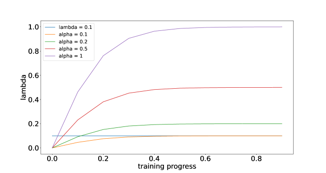
Figure 8: Functions for the gradient reversal coefficient $\lambda$.

Appendix 0.C LiDAR sensors details

In Table 9 we compare different LiDARs’s properties, their number of points per scan as well as height above ground in the different datasets. The variety of scenarios we tested clearly shows robustness of our and different UDA approaches, specifically when applied towards sparser data with large domain gaps. Comprehensive data analysis is available in the main paper (Section 4).

Table 9: LiDAR sensors details.

Sensor	FOV	$n_{points}/$ scan	LiDAR Height
HLD-64 (Kitti)	$26.9^{\circ}$	$\approx 118000$	$\approx 1.6$ m
VLD-64 (CS64)	$26.9^{\circ}$	$\approx 100000$	$\approx 2$ m
HLD-64 (Waymo)	$26.9^{\circ}$	$\approx 144512$	$\approx 1.6$ m
VLD-32 (CS32)	$40^{\circ}$	$\approx 63900$	$2$ m
VLD-32 (nuScenes)	$40^{\circ}$	$\approx 34688$	$1.6$ m
VLD-16 (CS16)	$30^{\circ}$	$\approx 22000$	$2$ m
VLP-16 (robot)	$30^{\circ}$	$\approx 22000$	$0.6$ m

Appendix 0.D Data Augmentation

0.D.1 Height shift

As highlighted in Section 4.1, there is a distinct difference in the LiDAR mounting height between different datasets. The LiDAR data in datasets are centered at sensor mounting positions, see Table 9. Following previous work for UDA in 3D object detection [58], the proposed method is combined with LiDAR height shift.

This transformation ensures that the ground plane of the source and target datasets is at the same LiDAR height of $0$ m. The shifted datasets are used simultaneously in the adaptation process, and any testing or inference is performed using the shifted point clouds.

0.D.2 Random Object Scaling

Random Object Scaling (ROS) applies random scaling factors to ground truth bounding boxes and their corresponding points. Each object point in ego-vehicle frame $(p_{i}^{x},p_{i}^{y},p_{i}^{z})_{\mathrm{ego}}$ is transformed to local object coordinates

$$\begin{array}[]{cc}(p_{i}^{l},p_{i}^{w},p_{i}^{h})_{\mathrm{object}}=((p_{i}^{x},p_{i}^{y},p_{i}^{z})_{\mathrm{ego}}-\\ ~{}~{}~{}~{}~{}~{}~{}~{}~{}~{}~{}~{}~{}~{}(c_{x},c_{y},c_{z})_{\mathrm{object}})\times R_{\mathrm{object}}\end{array}$$ (11)

where $(c_{x},c_{y},c_{z})_{\mathrm{object}}$ is object center coordinates and $R_{\mathrm{object}}$ is the rotation matrix between the ego-coordinates and object-coordinates. Each object point is then scaled by a random scaling factor $r$ drawn from a uniform random distribution:

$$\begin{array}[]{cc}(p_{i}^{l},p_{i}^{w},p_{i}^{h})_{\mathrm{object},\mathrm{scaled}}=r\cdot(p_{i}^{l},p_{i}^{w},p_{i}^{h})_{\mathrm{object}}\\ r\in U(r_{\mathrm{min}},r_{\mathrm{max}}).\end{array}$$ (12)

Afterwards, each object is transformed back into the ego-vehicle frame. The length $l$, width $w$, and height $h$ of each bounding box are also scaled accordingly with $r$.

Following previous works [48, 35, 58] experiments are performed by including object scaling in the source-data to account for different vehicle sizes. As examined in Section 4.1 there is a large difference between the vehicle sizes in LiDAR-CS, corresponding to large vehicle sizes typically found in the USA, and the smaller vehicles in Europe encountered by the robot, which encounters the smaller vehicles in Europe. Specifically, ROS from ST3D [58] is utilized where the objects and corresponding bounding boxes are scaled according to uniform noise in a chosen scaling interval. While previous UDA methods on LiDAR-based 3D object detection often apply domain adaptation only to a single object category, we consider it a multiclass problem. Therefore, ROS is used for all three classes (Vehicle, Pedestrian, and Cyclist) with different scaling intervals, shown in Table 10. The results of different scaling intervals are shown in Table 11. We can see that the best setting is $\Delta_{x,y,z}\in\{0.80,1.20\}$ for vehicles and $\Delta_{x,y,z}\in\{0.9,1.1\}$ for pedestrians and cyclists, thus, we chose this for all of our experiments.

Table 10: Tested multi-class scaling intervals for ROS.

Scaling	Vehicles	Pedestrians	Cyclists
Settings
1	$U(0.8,1.0)$	$U(0.8,1.0))$	$U(0.8,1.0)$
2	$U(0.9,1.1)$	$U(0.8,1.2)$	$U(0.8,1.2)$
3	$U(0.8,1.2)$	$U(0.9,1.1)$	$U(0.9,1.1)$

Table 11: Random Object Scaling using different scaling ranges tested on CS-16 $\rightarrow$ Robot.

	Source	$v_{0.8,1.0}$	$v_{0.8,1.2}$	$v_{0.9,1.1}$
	Only	$pc_{0.8,1.0}$	$pc_{.8,1.2}$	$pc_{0.9,1.1}$
$AP_{3D,V}$	28.96	46.17	50.83	44.66
$AP_{3D,P}$	11.26	37.39	40.36	39.36
$AP_{3D,C}$	4.99	31.22	30.23	25.76
$mAP_{3D}$	15.07	38.73	41.47	39.93

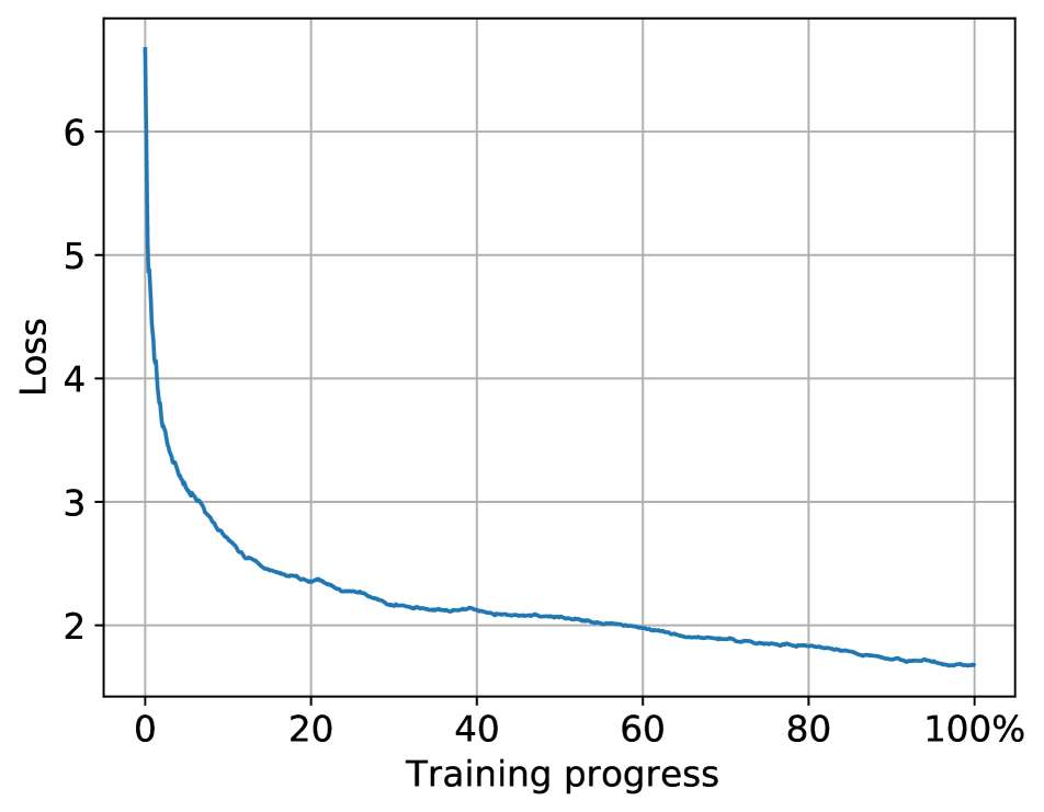
(a) Detection Loss.

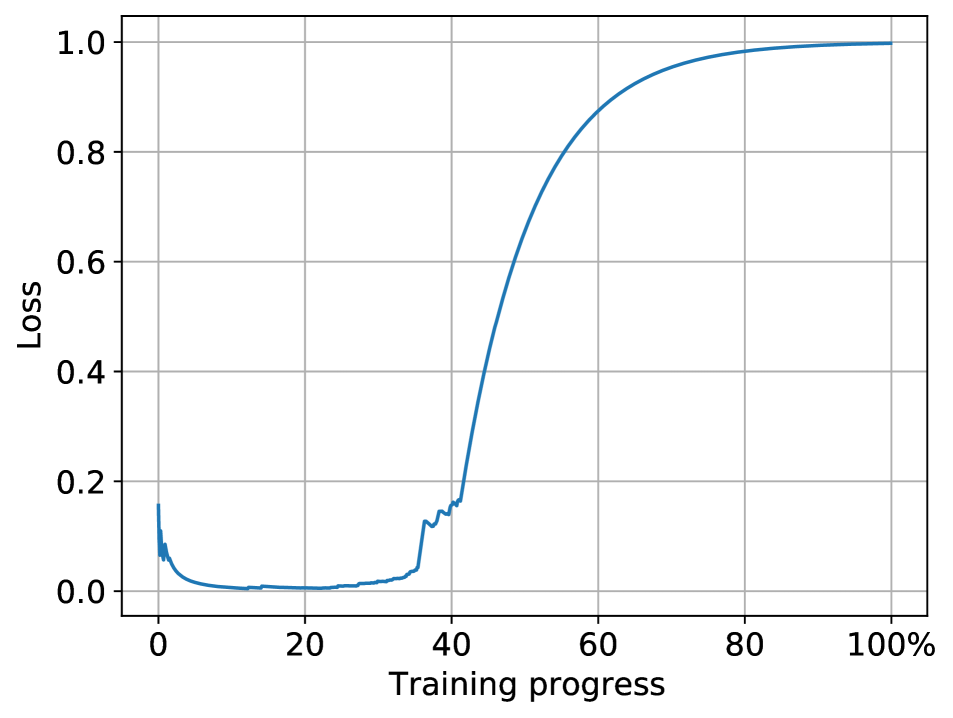
(b) Discriminators Loss.

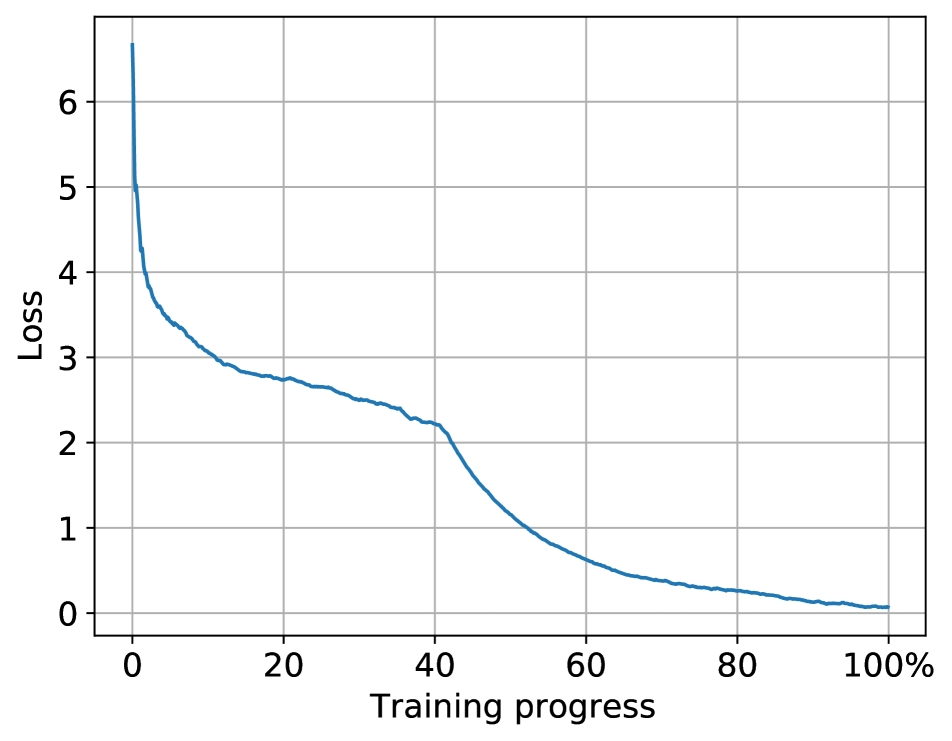
(c) Network loss.

Figure 9: Different losses in UADA3D.

Table 12: Comparison of performance of different adaptation scenario on sparse to dense task. $mAP_{3D/BEV}$ reported over 3 classes: Vehicle, Pedestrian, and Cyclist.

	CS64 →N (Centerpoint [63])		N →R(Centerpoint [63])
	3D/BEV	Closed Gap	3D/BEV	Closed Gap
Source	15.96/17.87	-/-	7.45/33.39	-/-
ST3D++	24.62/24.91	25.49%/ 22.49%	13.69/38.58	15.24%/ 9.46%
DTS	24.99/25.99	26.46%/25.29%	11.25/24.75	9.29%/-50.29%
L.D.	21.21/27.98	19.12%/30.46%	16.00/38.50	20.89%/13.44%
MS3D++	26.43/28.11	30.26%/ 30.80%	15.51/38.73	19.70%/ 10.11%
UADA3D	26.66/30.80	30.87%/ 37.78%	16.77/39.87	22.76%/ 15.01%
Oracle	52.84/54.77	-/-	48.39/59.54	-/-

0.D.3 Additional augmentation details

In addition to all the augmentation approaches described above, all methods were trained using standard LiDAR augmentation techniques that do not rely on ground truth bounding boxes. These augmentations are made up of random world flip in $x$ and $y$ directions, random world rotation around the $z$-axis in the range of $\{-\frac{\pi}{4},\frac{\pi}{4}\}$, and random world scaling in the range of $\{0.95,1.05\}$.

Appendix 0.E Loss analysis

The loss of our network consists of 2 components: detection loss and discriminator loss. While we optimize the discriminators with $\mathcal{L}_{C}$, we backpropagate this loss through the gradient reversal layer to the rest of the network. Thus, while the discriminator’s objective is to minimize $\mathcal{L}_{C}$, the feature extractor and detection head benefit from maximizing $\mathcal{L}_{C}$. In other words, the network aims to create features that are domain-invariant and useful for the object detection task. We can observe these losses in Fig. 9. Initially, we can see that the discriminator is capable of distinguishing between the domains as the loss decreases and approaches 0. However, after approximately 30% of the training, the network begins to produce more invariant features. By about 40% of the training, the network has learned to generate invariant features, leading to a rapid increase in conditional discriminator loss. These features are still beneficial for detection, resulting in a decrease in detection loss and a rapid overall loss reduction until the conditional discriminator loss plateaus again.

Appendix 0.F Additional experiments

0.F.1 Additional scenarios

In Table 12 we show additional comparisons of Centerpoint on adaptation from CS64 $\rightarrow$ N (sim-to-real) and N $\rightarrow$ R (autonomous driving data to robot) for the SOTA methods we used in the main paper. We can see that UADA3D again performs the best in this scenario.

0.F.2 Comparisons with other SOTA methods

For the sake of space, our paper concentrates on four SOTA unsupervised domain adaptation (UDA) methods. Specifically, our focus lies on those methods that either embody the original and pioneering approach (ST3D++), or have been explicitly focusing and tested on very sparse data (DTS and L.D.). MS3D++ uses ensemble of detectors, thus we hypothesised that it could have an advantage with challenging scenarios. MS3D++ was also one of few methods that reports adaptation between both Car and Pedestrian Classes. Below we present comparisons we additional SOTA methods. We focus on Waymo, KITTI and nuScenes datasets since these methods do not offer adaptation to custom datasets.

ReDB: We also compare with ReDB (ICCV ’23)  [4], one of few methods that consider adaptation to 3 classes as we do. We could see that ReBD achieved 32.12/28.56, 22.54/19.11 31.19/26.32 $AP~{}BEV/3D$ for Vehicle, Pedestrian and Cyclist on W$\rightarrow$N, while UADA3D 37.84/32.55, 23.49/21.23, 30.68/26.80 on Centerpoint adaptation. We can see that we only perform slightly worse on Cyclist adaptation, while we exceed on all the other classes and overall performance. We observed similar behavior when comparing N$\rightarrow$K adaptation, however here the difference was in the Vehicle class, where ReDB performed better on BEV metric but worse on AP3D, and its overall performance was 46.17/20.27, while UADA3D achieved 48.52/21.97 for $AP~{}BEV/3D$. Thus, we can see that our method generalize better across different categories.

Bi3D: Bi3D (CVPR ’23) [64], which is a semi-supervised learning method only focused on the Car Class. We still achieved better $AP~{}BEV/3D_{Vehicle}$ than them in W$\rightarrow$N adaptation: UADA3D 37.84/32.55 vs. Bi3D 35.29/30.81 (with $1\%$ of labeled target samples). On N $\rightarrow$ K, however, UADA3D achieved 65.24/25.34, and Bi3D 60.11/33.48, thus better than us on $AP3D_{Vehicle}$ metric However, as suspected, Bi3D further increases its performance if we increase labeled target samples percentage to $5\%$, since our method is fully unsupervised (no target labels during training).

0.F.3 Few shot learning

Motivated by other works, we try to use a few labels from target data to see if that can further improve our results. In Table 13, we present results across three scenarios. Interestingly, we observed some improvements, particularly in adaptation towards robot data, and slight enhancements in other datasets, although not as pronounced. This could be attributed to robot data being smaller than nuScenes. Notably, we observed particularly high improvements in the Pedestrian and Cyclist classes. Moreover, we found that adding W $\rightarrow$ N led to higher improvements than CS64 $\rightarrow$ N. Remarkably, we achieved these results using only 20 labeled target examples for this few-shot approach.

Table 13: Few-shot test on adapting Centerpoint using UADA3D. Results are reported for $AP_{3D}/AP_{BEV}$ over 3 classes.

Adaptation Scenario	Source only	UADA3D	Few Shot	Oracle
W $\rightarrow$ N	15.96 / 17.87	26.89 / 30.67	30.70/35.69	52.84 / 54.77
CS64 $\rightarrow$ N	14.97/16.24	26.66/30.80	27.03/30.24	52.84 / 54.77
N $\rightarrow$ R	7.45/33.39	16.77/39.87	26.45/41.46	48.39/59.54

Appendix 0.G Mobile Robot

0.G.1 Robot Setup

The mobile robot used to capture robot data is a wheeled last-mile delivery robot developed at TU Hamburg (see Figure 10). It is equipped with a Intel Core i7-7600U 2x2.80 GHz CPU and a NVIDIA Volta GPU with 64 Tensor cores. Its sensors consist of two forward and backward facing Stereolabs ZED2 stereo cameras, four Intel RealSense D435 stereo cameras in the downward direction as well as a 16-channel Velodyne Puck (VLP-16) LiDAR. Since this work concerns LiDAR-based detection, only the LiDAR sensor is used for detection in this work.

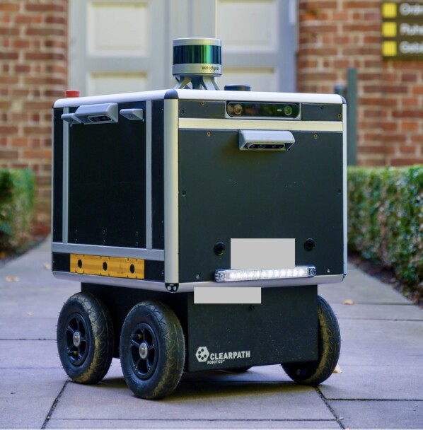
Figure 10: Sidewalk delivery robot prototype used for robot data recording.

0.G.2 Robot Data

The training data was collected at the campuses and the neighborhoods During training and testing the data was randomly sampled from these two locations. Our dataset includes sequences from both outdoor (university sidewalks, small university roads, or parking lots) and indoor (the university building and a warehouse) scenarios. Most of the objects classes in these areas are pedestrians and cyclists. There are also numerous vehicles, mostly parked on the side of the road or driving across the university campus. Since the data was collected in scenarios similar to the intended use cases for such robots it can be seen as an accurate representation of the data that would be encountered in real-world operation. The data was labeled using the open-source annotation software SUSTechPoints [21]. In our train/test split, we used a similar number of scans as on the KITTI [9] data. We used 7000 scans for training and 3500 for testing.

Together with this paper, we are planning to release the robot data we used in our scenarios. The complete dataset is a part of another project and will be published soon. In addition to the LiDAR data and class labels (used in this project), the full dataset will also include data from an RGBD camera, ground-facing stereo camera, an Inertial Measurement Unit (IMU), wheel odometry, and RTK GNSS. This diverse collection of sensors will offer a comprehensive perspective on the robot’s perception of its environment, providing valuable insights into the subtle aspects of robotic sensing capabilities.

Appendix 0.H Qualitative results

Our method, UADA3D, demonstrated the ability to accurately train the model to recognize objects, irrespective of their proximity and domain. This enhanced detection capability is effective across all three classes: vehicles, pedestrians, and cyclists. Our approach significantly improves the model’s ability to identify distant, close-by as well as heavily occluded objects. In the next figures, red bounding boxes indicate predictions, while green bounding boxes represent ground truth. We added blue squares to highlight zoomed-in regions, and yellow dotted squares to highlight hard-to-detect far-away objects. As illustrated in Figs. 12, 14 and 15, most of the models in comparison tend to miss far-away or partially occluded objects, without producing many false positives. Additionally, they also tend to miss smaller non-vehicle objects. UADA3D on the other hand substantially enhances the model’s robustness in these challenging scenarios, ensuring that such objects are not overlooked. Our method detects not only close and far away vehicles (Figs. 12, 14 and 15) but also hard-to-see cyclists and pedestrians (zoomed-in regions in Fig. 12 and Fig. 14, as well as highlighted with the yellow box containing one instance in Fig. 12). Moreover, in Fig. 16, which presents results on robot data, we show UADA3D’s comprehensive adaptation capabilities, where we successfully identify every object in the scene, even though the domain gap is substantially large (self-driving car domain to mobile robot). This highlights the effectiveness of our approach in diverse and demanding real-world applications.

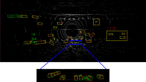
(a) UADA3D (ours)

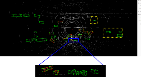
(b) ST3D++ [59]

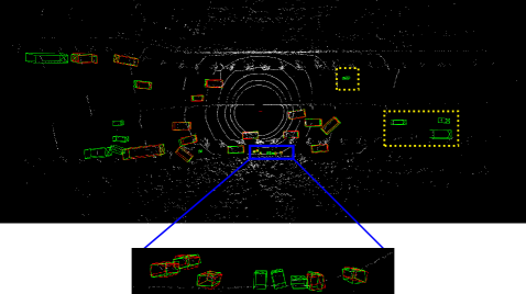
(c) DTS [14]

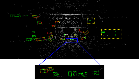
(a) L.D. [51]

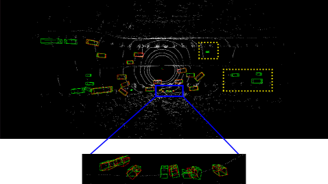
(b) MS3D++ [42]

Figure 12: Qualitative results CS64-CS16. Red bounding boxes indicate predictions, while green bounding boxes represent ground truth. We added a blue square to highlight zoomed-in regions, and the yellow dotted squares to highlight hard-to-detect far-away objects. Note that UADA3D is able to detect the pedestrians close by as well as the far-away objects, significantly reducing the number of missed detections.

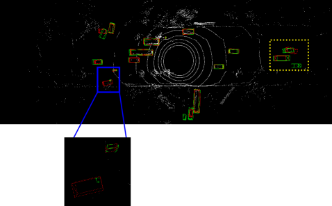
(a) UADA3D (ours)

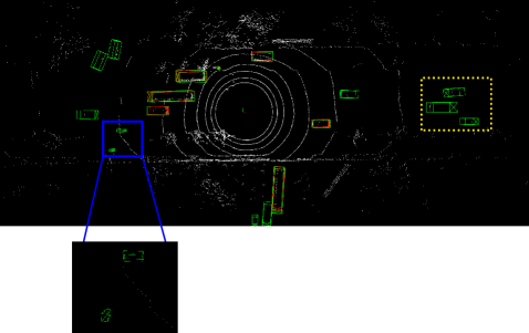
(b) ST3D++ [59]

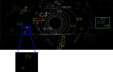
(c) DTS [14]

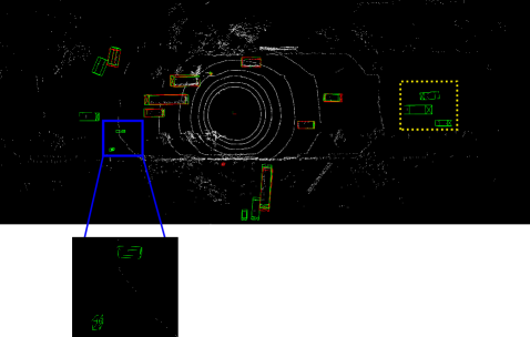
(a) L.D. [51]

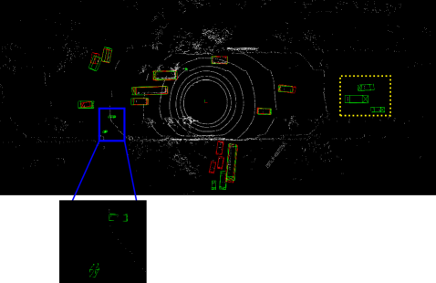
(b) MS3D++ [42]

Figure 14: Qualitative results CS64-CS16. Red bounding boxes indicate predictions, while green bounding boxes represent ground truth. We added a blue square to highlight zoomed-in regions, and the yellow dotted squares to highlight hard-to-detect far-away objects. Note that UADA3D is able to detect the pedestrians close by as well as the far-away objects, significantly reducing the number of missed detections.

(a) UADA3D (ours)

(b) ST3D++ [59]

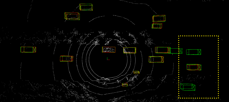
(c) DTS [14]

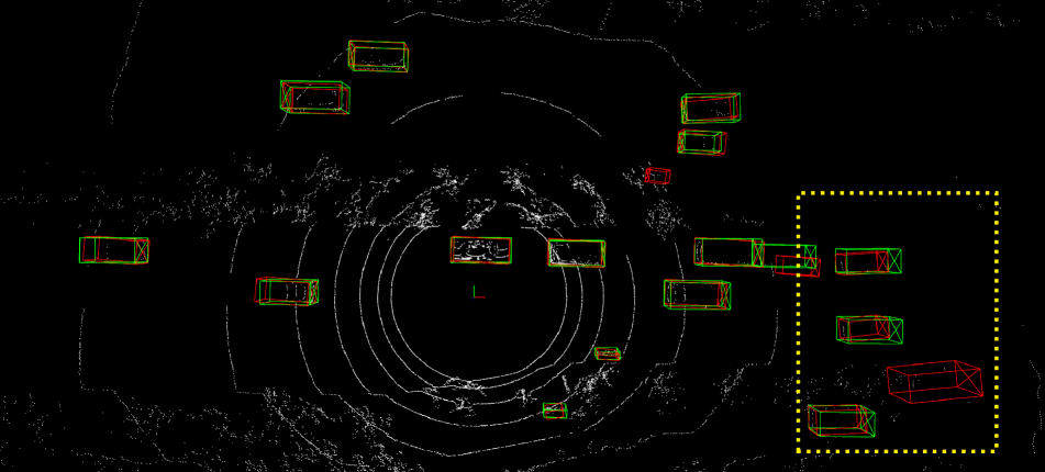
(d) L.D. [51]

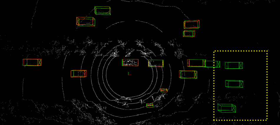
(e) MS3D++ [42]

Figure 15: Qualitative results CS64-CS16. Red bounding boxes indicate predictions, while green bounding boxes represent ground truth. Note that UADA3D is able to detect the pedestrians close by as well as the far-away objects, significantly reducing the number of missed detections.

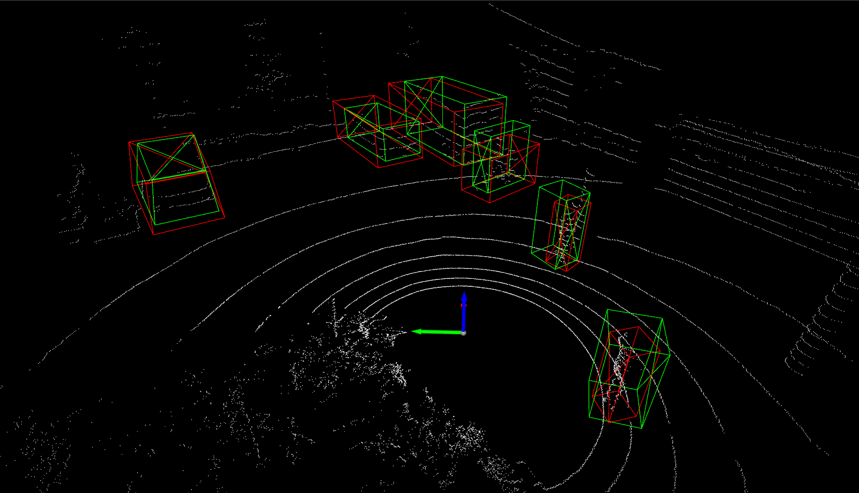
(a) UADA3D (ours)

(b) ST3D++ [59]

(c) DTS [14]

(d) L.D. [51]

(e) MS3D++ [42]

Figure 16: Qualitative results CS64-Robot. Red bounding boxes indicate predictions, while green bounding boxes represent ground truth. Note that UADA3D is able to detect the pedestrians close by as well as the far-away objects, significantly reducing the number of missed detections.

References

- [1] X. Bai, Z. Hu, X. Zhu, Q. Huang, Y. Chen, H. Fu, and C.-L. Tai. Transfusion: Robust lidar-camera fusion for 3d object detection with transformers. In Proceedings of the IEEE/CVF Conference on Computer Vision and Pattern Recognition, pages 1090–1099, 2022.
- [2] H. Caesar, V. Bankiti, A. H. Lang, S. Vora, V. E. Liong, Q. Xu, A. Krishnan, Y. Pan, G. Baldan, and O. Beijbom. nuscenes: A multimodal dataset for autonomous driving. In Proceedings of the IEEE/CVF Conference on Computer Vision and Pattern Recognition, pages 11621–11631, 2020.
- [3] Y. Chen, W. Li, C. Sakaridis, D. Dai, and L. Van Gool. Domain adaptive faster r-cnn for object detection in the wild. In Proceedings of the IEEE/CVF Conference on Computer Vision and Pattern Recognition, pages 3339–3348, 2018.
- [4] Z. Chen, Y. Luo, Z. Wang, M. Baktashmotlagh, and Z. Huang. Revisiting domain-adaptive 3d object detection by reliable, diverse and class-balanced pseudo-labeling. In Proceedings of the International Conference on Computer Vision, pages 3714–3726, 2023.
- [5] R. DeBortoli, L. Fuxin, A. Kapoor, and G. A. Hollinger. Adversarial training on point clouds for sim-to-real 3d object detection. IEEE Robotics and Automation Letters, 6(4):6662–6669, 2021.
- [6] J. Fang, D. Zhou, J. Zhao, C. Tang, C.-Z. Xu, and L. Zhang. Lidar-cs dataset: Lidar point cloud dataset with cross-sensors for 3d object detection. arXiv preprint arXiv:2301.12515, 2023.
- [7] T. Feng, H. Shi, X. Liu, W. Feng, L. Wan, Y. Zhou, and D. Lin. Open compound domain adaptation with object style compensation for semantic segmentation. Advances in Neural Information Processing Systems, 36, 2024.
- [8] Y. Ganin and V. Lempitsky. Unsupervised domain adaptation by backpropagation. In International Conference on Machine Learning, pages 1180–1189. PMLR, 2015.
- [9] A. Geiger, P. Lenz, C. Stiller, and R. Urtasun. Vision meets robotics: The kitti dataset. The International Journal of Robotics Research, 2013.
- [10] C. He, H. Zeng, J. Huang, X.-S. Hua, and L. Zhang. Structure aware single-stage 3d object detection from point cloud. In Proceedings of the IEEE/CVF Conference on Computer Vision and Pattern Recognition, pages 11873–11882, 2020.
- [11] Z. He and L. Zhang. Multi-adversarial faster-rcnn for unrestricted object detection. In Proceedings of the International Conference on Computer Vision, pages 6668–6677, 2019.
- [12] D. Hegde, V. Sindagi, V. Kilic, A. B. Cooper, M. Foster, and V. Patel. Uncertainty-aware mean teacher for source-free unsupervised domain adaptive 3d object detection. arXiv preprint arXiv:2109.14651, 2021.
- [13] J. Hoffman, E. Tzeng, T. Park, J.-Y. Zhu, P. Isola, K. Saenko, A. Efros, and T. Darrell. Cycada: Cycle-consistent adversarial domain adaptation. In International Conference on Machine Learning, pages 1989–1998. Pmlr, 2018.
- [14] Q. Hu, D. Liu, and W. Hu. Density-insensitive unsupervised domain adaption on 3d object detection. In Proceedings of the IEEE/CVF Conference on Computer Vision and Pattern Recognition, pages 17556–17566, 2023.
- [15] C. Huang, V. Abdelzad, S. Sedwards, and K. Czarnecki. Soap: Cross-sensor domain adaptation for 3d object detection using stationary object aggregation pseudo-labelling. In Proceedings of the IEEE/CVF Winter Conference on Applications of Computer Vision, pages 3352–3361, 2024.
- [16] K.-C. Huang, T.-H. Wu, H.-T. Su, and W. H. Hsu. Monodtr: Monocular 3d object detection with depth-aware transformer. In Proceedings of the IEEE/CVF Conference on Computer Vision and Pattern Recognition, pages 4012–4021, 2022.
- [17] M. Jaritz, T.-H. Vu, R. d. Charette, E. Wirbel, and P. Pérez. xmuda: Cross-modal unsupervised domain adaptation for 3d semantic segmentation. In Proceedings of the IEEE/CVF conference on computer vision and pattern recognition, pages 12605–12614, 2020.
- [18] D. P. Kingma and J. Ba. Adam: A method for stochastic optimization. arXiv preprint arXiv:1412.6980, 2014.
- [19] L. Kong, N. Quader, and V. E. Liong. Conda: Unsupervised domain adaptation for lidar segmentation via regularized domain concatenation. In 2023 IEEE International Conference on Robotics and Automation (ICRA), pages 9338–9345. IEEE, 2023.
- [20] A. H. Lang, S. Vora, H. Caesar, L. Zhou, J. Yang, and O. Beijbom. Pointpillars: Fast encoders for object detection from point clouds. In Proceedings of the IEEE/CVF Conference on Computer Vision and Pattern Recognition, pages 12697–12705, 2019.
- [21] E. Li, S. Wang, C. Li, D. Li, X. Wu, and Q. Hao. Sustech points: A portable 3d point cloud interactive annotation platform system. In 2020 IEEE Intelligent Vehicles Symposium (IV), pages 1108–1115, 2020.
- [22] J. Li, R. Xu, J. Ma, Q. Zou, J. Ma, and H. Yu. Domain adaptive object detection for autonomous driving under foggy weather. In Proceedings of the IEEE/CVF Conference on Computer Vision and Pattern Recognition, pages 612–622, 2023.
- [23] R. Li, Q. Jiao, W. Cao, H.-S. Wong, and S. Wu. Model adaptation: Unsupervised domain adaptation without source data. In Proceedings of the IEEE/CVF Conference on Computer Vision and Pattern Recognition, pages 9641–9650, 2020.
- [24] Z. Li, J. Guo, T. Cao, L. Bingbing, and W. Yang. Gpa-3d: Geometry-aware prototype alignment for unsupervised domain adaptive 3d object detection from point clouds. In Proceedings of the International Conference on Computer Vision, pages 6394–6403, 2023.
- [25] T. Liang, H. Xie, K. Yu, Z. Xia, Z. Lin, Y. Wang, T. Tang, B. Wang, and Z. Tang. Bevfusion: A simple and robust lidar-camera fusion framework. Advances in Neural Information Processing Systems, 35:10421–10434, 2022.
- [26] Y. Liao, W. Zhou, X. Yan, Z. Li, Y. Yu, and S. Cui. Geometry-aware network for domain adaptive semantic segmentation. In Proceedings of the AAAI Conference on Artificial Intelligence, volume 37, pages 8755–8763, 2023.
- [27] X. Liu, Z. Guo, S. Li, F. Xing, J. You, C.-C. J. Kuo, G. El Fakhri, and J. Woo. Adversarial unsupervised domain adaptation with conditional and label shift: Infer, align and iterate. In Proceedings of the IEEE/CVF Conference on Computer Vision and Pattern Recognition, pages 10367–10376, 2021.
- [28] Z. Liu, H. Tang, A. Amini, X. Yang, H. Mao, D. L. Rus, and S. Han. Bevfusion: Multi-task multi-sensor fusion with unified bird’s-eye view representation. In Proceedings of the IEEE International Conference on Robotics and Automation, pages 2774–2781. IEEE, 2023.
- [29] Z. Luo, Z. Cai, C. Zhou, G. Zhang, H. Zhao, S. Yi, S. Lu, H. Li, S. Zhang, and Z. Liu. Unsupervised domain adaptive 3d detection with multi-level consistency. In Proceedings of the International Conference on Computer Vision, pages 8866–8875, 2021.
- [30] T.-M. Nguyen, S. Yuan, T. H. Nguyen, P. Yin, H. Cao, L. Xie, M. Wozniak, P. Jensfelt, M. Thiel, J. Ziegenbein, et al. Mcd: Diverse large-scale multi-campus dataset for robot perception. arXiv preprint arXiv:2403.11496, 2024.
- [31] A. Paigwar, D. Sierra-Gonzalez, Ö. Erkent, and C. Laugier. Frustum-pointpillars: A multi-stage approach for 3d object detection using rgb camera and lidar. In Proceedings of the International Conference on Computer Vision, pages 2926–2933, 2021.
- [32] X. Peng, X. Zhu, and Y. Ma. Cl3d: Unsupervised domain adaptation for cross-lidar 3d detection. In Proceedings of the AAAI Conference on Artificial Intelligence, volume 37, pages 2047–2055, 2023.
- [33] C. R. Qi, H. Su, K. Mo, and L. J. Guibas. Pointnet: Deep learning on point sets for 3d classification and segmentation. In Proceedings of the IEEE/CVF Conference on Computer Vision and Pattern Recognition, pages 652–660, 2017.
- [34] K. Saito, Y. Ushiku, T. Harada, and K. Saenko. Strong-weak distribution alignment for adaptive object detection. In Proceedings of the IEEE/CVF Conference on Computer Vision and Pattern Recognition, pages 6956–6965, 2019.
- [35] C. Saltori, S. Lathuiliere, N. Sebe, E. Ricci, and F. Galasso. Sf-uda 3d: Source-free unsupervised domain adaptation for lidar-based 3d object detection. In Proceedings of the International Conference on 3D Vision (3DV), pages 771–780. IEEE, 2020.
- [36] M. Schutera, M. Hussein, J. Abhau, R. Mikut, and M. Reischl. Night-to-day: Online image-to-image translation for object detection within autonomous driving by night. IEEE Transactions on Intelligent Vehicles, 6(3):480–489, 2021.
- [37] S. Shi, X. Wang, and H. Li. Pointrcnn: 3d object proposal generation and detection from point cloud. In Proceedings of the IEEE/CVF Conference on Computer Vision and Pattern Recognition, pages 770–779, 2019.
- [38] R. Siegwart, I. R. Nourbakhsh, and D. Scaramuzza. Introduction to autonomous mobile robots. MIT press, 2011.
- [39] P. Sun, H. Kretzschmar, X. Dotiwalla, A. Chouard, V. Patnaik, P. Tsui, J. Guo, Y. Zhou, Y. Chai, B. Caine, et al. Scalability in perception for autonomous driving: Waymo open dataset. In Proceedings of the IEEE/CVF Conference on Computer Vision and Pattern Recognition, pages 2446–2454, 2020.
- [40] O. D. Team. Openpcdet: An open-source toolbox for 3d object detection from point clouds. https://github.com/open-mmlab/OpenPCDet, 2020.
- [41] C.-Y. Tsai, H. Nisar, and Y.-C. Hu. Mapless lidar navigation control of wheeled mobile robots based on deep imitation learning. IEEE Access, 9:117527–117541, 2021.
- [42] D. Tsai, J. S. Berrio, M. Shan, E. Nebot, and S. Worrall. Ms3d: Leveraging multiple detectors for unsupervised domain adaptation in 3d object detection. In International Conference on Intelligent Transportation Systems. IEEE, 2023.
- [43] D. Tsai, J. S. Berrio, M. Shan, S. Worrall, and E. Nebot. See eye to eye: A lidar-agnostic 3d detection framework for unsupervised multi-target domain adaptation. IEEE Robotics and Automation Letters, 7(3):7904–7911, 2022.
- [44] V. Vidit and M. Salzmann. Attention-based domain adaptation for single-stage detectors. Machine Vision and Applications, 33(5):1–14, 2022.
- [45] V. VS, P. Oza, and V. M. Patel. Towards online domain adaptive object detection. In Proceedings of the IEEE Winter Conference on Applications of Computer Vision, pages 478–488, 2023.
- [46] T.-H. Vu, H. Jain, M. Bucher, M. Cord, and P. Pérez. Advent: Adversarial entropy minimization for domain adaptation in semantic segmentation. In Proceedings of the IEEE/CVF conference on computer vision and pattern recognition, pages 2517–2526, 2019.
- [47] T. Wang, J. Pang, and D. Lin. Monocular 3d object detection with depth from motion. In Proceedings of the European Conference on Computer Vision, pages 386–403. Springer, 2022.
- [48] Y. Wang, X. Chen, Y. You, L. E. Li, B. Hariharan, M. Campbell, K. Q. Weinberger, and W.-L. Chao. Train in germany, test in the usa: Making 3d object detectors generalize. In Proceedings of the IEEE/CVF Conference on Computer Vision and Pattern Recognition, pages 11710–11720, 2020.
- [49] Y. Wang, J. Yin, W. Li, P. Frossard, R. Yang, and J. Shen. Ssda3d: Semi-supervised domain adaptation for 3d object detection from point cloud. In Proceedings of the AAAI Conference on Artificial Intelligence, volume 37, pages 2707–2715, 2023.
- [50] Z. Wang, L. Wang, L. Xiao, and B. Dai. Unsupervised subcategory domain adaptive network for 3d object detection in lidar. Electronics, 10(8):927, 2021.
- [51] Y. Wei, Z. Wei, Y. Rao, J. Li, J. Zhou, and J. Lu. Lidar distillation: Bridging the beam-induced domain gap for 3d object detection. In Proceedings of the European Conference on Computer Vision, pages 179–195. Springer, 2022.
- [52] B. Wilson, W. Qi, T. Agarwal, J. Lambert, J. Singh, S. Khandelwal, B. Pan, R. Kumar, A. Hartnett, J. K. Pontes, D. Ramanan, P. Carr, and J. Hays. Argoverse 2: Next generation datasets for self-driving perception and forecasting. In NeurIPS, 2021.
- [53] M. K. Wozniak, V. Karefjard, M. Hansson, M. Thiel, and P. Jensfelt. Applying 3d object detection from self-driving cars to mobile robots: A survey and experiments. In 2023 IEEE International Conference on Autonomous Robot Systems and Competitions (ICARSC), pages 3–9. IEEE, 2023.
- [54] M. K. Wozniak, V. Kårefjärd, M. Thiel, and P. Jensfelt. Towards a robust sensor fusion step for 3d object detection on corrupted data. IEEE Robotics and Automation Letters, 2023.
- [55] C.-D. Xu, X.-R. Zhao, X. Jin, and X.-S. Wei. Exploring categorical regularization for domain adaptive object detection. In Proceedings of the IEEE/CVF Conference on Computer Vision and Pattern Recognition, pages 11724–11733, 2020.
- [56] Q. Xu, Y. Zhou, W. Wang, C. R. Qi, and D. Anguelov. Spg: Unsupervised domain adaptation for 3d object detection via semantic point generation. In Proceedings of the International Conference on Computer Vision, pages 15446–15456, 2021.
- [57] Y. Yan, Y. Mao, and B. Li. Second: Sparsely embedded convolutional detection. Sensors, 18(10):3337, 2018.
- [58] J. Yang, S. Shi, Z. Wang, H. Li, and X. Qi. St3d: Self-training for unsupervised domain adaptation on 3d object detection. In Proceedings of the IEEE/CVF Conference on Computer Vision and Pattern Recognition, pages 10368–10378, 2021.
- [59] J. Yang, S. Shi, Z. Wang, H. Li, and X. Qi. St3d++: Denoised self-training for unsupervised domain adaptation on 3d object detection. IEEE Transactions on Pattern Analysis and Machine Intelligence, 45(5):6354–6371, 2022.
- [60] Z. Yang, Y. Sun, S. Liu, and J. Jia. 3dssd: Point-based 3d single stage object detector. In Proceedings of the IEEE/CVF Conference on Computer Vision and Pattern Recognition, pages 11040–11048, 2020.
- [61] Z. Yang, Y. Sun, S. Liu, X. Shen, and J. Jia. Std: Sparse-to-dense 3d object detector for point cloud. In Proceedings of the International Conference on Computer Vision, pages 1951–1960, 2019.
- [62] L. Yi, B. Gong, and T. Funkhouser. Complete & label: A domain adaptation approach to semantic segmentation of lidar point clouds. In Proceedings of the IEEE/CVF conference on computer vision and pattern recognition, pages 15363–15373, 2021.
- [63] T. Yin, X. Zhou, and P. Krahenbuhl. Center-based 3d object detection and tracking. In Proceedings of the IEEE/CVF Conference on Computer Vision and Pattern Recognition, pages 11784–11793, 2021.
- [64] J. Yuan, B. Zhang, X. Yan, T. Chen, B. Shi, Y. Li, and Y. Qiao. Bi3d: Bi-domain active learning for cross-domain 3d object detection. In Proceedings of the IEEE/CVF Conference on Computer Vision and Pattern Recognition, pages 15599–15608, 2023.
- [65] B. Zhang, T. Chen, B. Wang, and R. Li. Joint distribution alignment via adversarial learning for domain adaptive object detection. IEEE Transactions on Multimedia, 24:4102–4112, 2021.
- [66] Y. Zhang, Q. Hu, G. Xu, Y. Ma, J. Wan, and Y. Guo. Not all points are equal: Learning highly efficient point-based detectors for 3d lidar point clouds. In Proceedings of the IEEE/CVF Conference on Computer Vision and Pattern Recognition, pages 18953–18962, 2022.
- [67] Y. Zhou and O. Tuzel. Voxelnet: End-to-end learning for point cloud based 3d object detection. In Proceedings of the IEEE/CVF Conference on Computer Vision and Pattern Recognition, pages 4490–4499, 2018.
sec0em1.7em \cftsetindentssubsec1.2em2.35em Supplementary Material ECCV 2024 #7127