A new construction of modified equations for variational integrators
Abstract
The construction of modified equations is an important step in the backward error analysis of symplectic integrator for Hamiltonian systems. In the context of partial differential equations, the standard construction leads to modified equations with increasingly high frequencies which increase the regularity requirements on the analysis. In this paper, we consider the next order modified equations for the implicit midpoint rule applied to the semilinear wave equation to give a proof-of-concept of a new construction which works directly with the variational principle. We show that a carefully chosen change of coordinates yields a modified system which inherits its analytical properties from the original wave equation. Our method systematically exploits additional degrees of freedom by modifying the symplectic structure and the Hamiltonian together.
In memory of Claudia Wulff
1 Introduction
Over the last decades, backward error analysis has emerged as a useful tool for proving conservation properties of numerical time integrators for differential equations. In a nutshell, one constructs a modified differential equation which is approximated by the numerical method to some higher order than the original equation and which possesses analogous conservation laws. Thus, the numerical scheme is nearly conservative on time scales over which it approximates the solution of the modified equation. Some of the strongest and most general results for ordinary differential equations were obtained by Benettin and Giorgilli [2] and Hairer and Lubich [15], using ideas which go back to Neishtadt [25], who optimally truncate an asymptotic series for the modified vector field to prove that a class of symplectic schemes when applied to Hamiltonian ordinary differential equations preserve the energy exponentially well over exponentially long times in the step size. Similar ideas appear in [16, 19, 32].
While this construction formally extends to Hamiltonian partial differential equations, in this case the asymptotic series for the modified equation will generally contain arbitrary powers of unbounded operators, thereby breaking the natural ordering of the terms in the asymptotic series. In particular, the standard construction in the context of hyperbolic equations such as the semilinear wave equation, fails in the practically relevant regime when the scaling of time vs. space step is close to the CFL limit. This problem has been partially addressed in a number of ways. Cano [5] proves an exponential backward error analysis result conditional on a number of conjectures. Moore and Reich [24] and Islas and Schober [18] provide a formal backward error analysis in a multisymplectic setting. Under strong regularity assumptions on the true solution, [29, 30, 37] show that the occurrence of unbounded operators in the modified vector field only leads to loss of order in the exponents of the backward error estimates. Sometimes, non-standard modified equations can be helpful, such as in the result of [28] on the approximate numerical preservation of the momentum invariant. Cohen, Hairer, and Lubich [6] obtained results on polynomially long times for full time-spectral discretization of weakly nonlinear wave equations using the method of modulated Fourier expansions. Finally, there is a large body of work on the backward error analysis of splitting methods applied to partial differential equations [9, 8, 10, 11, 12]. However, the question whether strong results for generic solutions, i.e. solutions which are neither small nor analytic, can be obtained remains open.
Modified equations are clearly not unique. Various expressions appearing beyond the leading order of the asymptotic series can be consistently replaced by using the modified equation itself. In principle, one can use such substitutions to remove the occurrence of high frequencies at high orders of the modified system. Unfortunately, this process will generally break the Hamiltonian structure.
This paper is motivated by the observation that a large class of symplectic integrators can be derived via a discrete variational principle. Elementary examples appear in Wendlandt and Marsden [36] and Marsden and West [22] who, in particular, show that the implicit midpoint rule arises via a simple finite difference approximation of the action integral. More generally, a large number of symplectic schemes arises as variational integrators [20, 22]; in particular, Leok and Zhang [21] show that it is also possible to obtain variational integrators on the Hamiltonian side, which extends the concept to systems with degenerate Hamiltonians. Vermeeren [33, 34] modified equations on the Lagrangian side, albeit only for finite dimensional systems and in the sense of so-called meshed Lagrangians. Recently, McLachlan and Offen [23] consider variational backward error analysis for symmetry solutions of wave equations. This reduction again specializes the problem to finite-dimensional modified equations. A variational treatment of the general case is, so far, open.
In this paper, we demonstrate that it is possible to construct modified equations via a classical variational principle. A naive variational construction has the drawback that the order of time derivatives in the modified equations increases with the order to which the modified equations are constructed, i.e., the phase space gets increasingly larger. Since the higher time derivatives appear at higher orders of the expansion (see e.g. [24, 23]), such constructions lead to singular perturbation problems with multiple fast time scales. Still, the original slow dynamics lives on a submanifold in this larger phase space. Our main point is that we can approximately restrict to this submanifold by the use of a near-identity change of variables which moves all fast degrees of freedom beyond the truncation order of the asymptotic expansion. We call this approach the method of degenerate variational asymptotics; it is motivated by earlier work on model reduction for rapidly rotating fluid flow [26, 27].
The current work is the first proof-of-concept for this approach. In the first part of the paper, we consider a simple, yet nontrivial special case: the next-order modified equations for the implicit midpoint scheme applied to the semilinear wave equation. We find that the new modified equations do not admit frequencies beyond the scale already present in the original partial differential equation. In particular, unlike the modified equations which arise from the conventional construction, they have a dispersion relation for linear waves which has a finite limit as the wave number tends to infinity. This behavior coincides qualitatively with that of the implicit midpoint rule itself, which also possesses a finite highest numerical frequency in a time-semidiscrete analysis [4]. Moreover, we can show that the full nonlinear modified equations are well-posed—locally in time but for a time interval which is independent of the time step parameter—precisely in the energy space which arises naturally from the modified Hamiltonian. In the second part of the paper, we show how to extend the approach to arbitrary high order. This part of the paper is formal, but we make sure that all spatial operators appearing in the final modified equations are bounded, and all such operators, except those that must limit to the second space derivative as , are bounded uniformly as a function of . We start with looking at the linear wave equation only, where an all-order modified equation can be found via a generating function approach. From there, we move to the nonlinear case where, up to an arbitrary but fixed order, we use a bilevel iterative concatenation of transformations to remove all higher-order time derivatives from the Lagrangian.
The paper is structured as follows. After the introduction of the semilinear wave equation in Section 2, Section 3 gives a brief derivation of the implicit midpoint scheme as a variational integrator. In Section 4, we recall the standard Hamiltonian construction of the modified vector field and show that the result is only useful under restrictive time-step assumptions. Section 5 explains the naive variational construction; Section 6 introduces the method of degenerate variational asymptotics, which constrains the phase space of the modified equations to the slow degrees of freedom. After addressing the question of consistent initialization of the modified system in Section 7, in Section 8 we give a numerical evidence that the new modified equations indeed perform as claimed. In Section 9, we present an analytic framework in which the nonlinear elliptic operator which arises in the formulation of the new modified equations is invertible, and we recast them in the form of a semilinear evolution equation, thereby obtaining a proof of local well-posedness in the natural energy space. Section 10 discusses the all-order modified equations for the linear wave equations, and Section 11 the subsequent extension to the nonlinear case. Finally, Section 12 concludes with a brief discussion of the results.
2 The semilinear wave equation
We consider the semilinear wave equation on the circle ,
| (1) |
where and we write . It arises as the Euler–Lagrange equation with Lagrangian given by
| (2) |
with and being a space of sufficiently smooth functions on ; we also assume that is smooth.
Writing , the semilinear wave equation is Hamiltonian with conserved energy
| (3) |
In addition, the Lagrangian is invariant under space translations. Hence, Noether’s theorem implies conservation of momentum
| (4) |
It is often convenient to write the semilinear wave equation as a first order system: setting
| (5) |
equation (1) takes the form
| (6) |
3 Variational integrators
Consider uniform grid on time interval with mesh size . Following [35, 36], we consider the discrete variational principle associated with the temporal semidiscretization, namely, find which are a stationary point of the discrete action
| (7) |
subject to variations which leave the temporal endpoints and fixed. The discrete variational principle yields the discrete Euler–Lagrange equation
| (8) |
for .
A symplectic scheme of second order for the semilinear wave equation is obtained by taking the discrete Lagrangian
| (9) |
Introducing the discrete Legendre transform [16, p. 194],
| (10) |
and using the discrete Euler–Lagrange equation (8), we obtain
| (11) |
The variations on the right of (10) and (11) read
| (12) |
where we identify with a subspace of via the inner product. We now introduce an intermediate integration stage via
| (13) |
Then, taking the sum and difference of (10) and (11), respectively, we obtain
| (14a) | |||
| (14b) | |||
Written in this form, the scheme is clearly recognized as the implicit midpoint rule, which is, in fact, a second order Gauss–Legendre Runge–Kutta method. To obtain a practical numerical scheme, it is better to replace the definition of the intermediate integration stage by the equivalent expressions [3]
| (15a) | |||
| (15b) | |||
In terms of the vector notation introduced at the end of Section 2, (15) reads
| (16) |
or
| (17) |
For sufficiently small and a suitable choice of function space, the operator on the right side of (17) is a contraction, so that the intermediate stage vector can be found iteratively.
Similarly, noting that , we can write (14) in the form
| (18) |
where
| (19) |
is known as the stability function of the method. Again, equation (18) considered, for instance, in a Sobolev space with has only bounded operators on its right hand side, so the time- map of the scheme does not lose derivatives. For this reason, the system (17) and (18) is the preferred form for numerical implementation of the implicit midpoint scheme.
4 Backward error analysis on the Hamiltonian side
In this section, we give an elementary derivation of the standard Hamiltonian modified equation which corresponds to the implicit midpoint rule up to terms of . The procedure is that of Hairer, Lubich, and Wanner [16, Chapter IX]; our presentation reduces the procedure to the special case at hand.
We use the following notation. Let be a curve satisfying an autonomous equation of the form
| (20) |
with for . Let us fix and Taylor expand about . On the one hand,
| (21) |
where , , and . On the other hand, is determined by the implicit midpoint rule
| (22) |
Since the implicit midpoint rule is a symmetric method, only terms at even powers of appear in the modified equation [16]. Therefore, to determine the modified equation including terms of , we seek a vector field such that
| (23) |
We note that (23) implies the approximate identities
| (24a) | |||
| (24b) | |||
Then, equating (21) and (22), using (23) and (24) to eliminate all derivatives, we obtain
| (25) |
In the particular case of the semilinear wave equation, where
| (26) |
we obtain by direct calculation that
| (27) |
Hence, the modified equation up to terms of order reads
| (28a) | |||
| (28b) | |||
It is straightforward to verify that modified equations (28) define a Hamiltonian system with Hamiltonian
| (29) |
It is generally true that symplectic Runge–Kutta schemes applied to Hamiltonian systems yield a Hamiltonian modified equation at any order [16, Section IX.3].
The difficulty with using the modified system (28) for the purpose of backward error analysis can be seen as follows. We consider, for simplicity, the linear case when . Writing to denote the spatial wave number, equation (6) in the space-frequency domain reads
| (30) |
We observe that the additional factor will introduce fast frequencies into the modified dynamics unless we restrict the admissible wave numbers and time steps. More generally, it can be shown that the modified vector field will be an asymptotic series in , so that the series will be properly ordered only if we restrict to a finite dimensional subspace of wave numbers—a discretization in space—and if . This excludes the practically relevant regime of time steps as large as permitted by the CFL condition where ; see, for example, the discussion in [6].
5 Backward error analysis on the Lagrangian side
We now turn to the question of how we can derive modified equations using the variational principle which underlies the semilinear wave equation.
The notation here is analogous to the notation used in the previous section: let be a curve in such that for . Again, we fix and Taylor expand and about . Then, for ,
| (31a) | |||
| (31b) | |||
where , , and . In particular, setting , we have
| (32) |
Substituting (32) into the discrete Lagrangian, we obtain
| (33) |
On the other hand, we may substitute the expansions (31) into the continuum action functional and collect terms containing identical powers of . We find that
| (34) |
Inserting the expanded discrete Lagrangian (33) into the discrete action (7) and comparing with (34), we find that
| (35) |
Integrating by parts with respect to time, we obtain—up to boundary terms which do not contribute to the variational principle because and are held fixed at the temporal endpoints—that
| (36) |
Thus, the discrete variational principle with Lagrangian is equivalent—up to terms of —to the continuous variational principle for the modified Lagrangian
| (37) |
We now seek stationary points of the modified action with respect to variation where and are held fixed at and . The resulting Euler–Lagrange equations read, abstractly,
| (38) |
This expression evaluates to
| (39) |
We note that this equation is of higher order with respect to time compared to the original semilinear wave equation, i.e., it has the form of a singular perturbation problem in a bigger phase space. As this is undesirable, we seek to restrict the modified dynamics to the phase space of the original equation.
In this simple example, this could be done ad hoc by using the second time derivative of the semilinear wave equation to eliminate the fourth time derivative from the modified equation—an approximation which gives a formally correct result. In this case, the resulting equation would only contain frequencies on the order of those already present in the original problem and, although non-variational, approximately preserve energy over long times. In the next section, we show that this can also be addressed by a systematic variational construction.
6 Method of degenerate variational asymptotics
We introduce a near-identity configuration space transformation of the general form
| (40) |
where denotes the solution curve in old physical configuration space coordinates and denotes the solution in a new coordinate system in which the modified equation will be computed. The field can be seen as the leading order generator of the transformation. It will be chosen a posteriori in such a way that the transformed modified Lagrangian (37), when truncated to , will not depend on time derivatives of order two and higher. We compute
| (41) |
We now observe that choosing , where is some functional acting on for fixed, we formally eliminate the excess time derivatives from the terms in (41). The choice of is, in principle, entirely free. It appears sensible, though, to consider only choices that are dimensionally consistent. Specializing further, two cases stand out. The apparently simplest choice is , so that
| (42) |
Alternatively, we might take
| (43) |
in which case vanishes formally up to terms of .
Inserting (42) into (41), integrating by parts, discarding all perfect time derivatives, and truncating to , we obtain the modified Lagrangian
| (44) |
We compute
| (45a) | ||||
| and | ||||
| (45b) | ||||
Hence, the transformed modified Euler–Lagrange equations read
| (46) |
The equations of motion conserve the energy
| (47) |
where denotes the -pairing between and .
We remark that the transformation we use as well as the resulting Hamiltonian are different from classic Hamiltonian normal form theory (see, e.g., [1] for a general exposition and [7] for an application of normal form theory to a fast-slow system with gyroscopic forcing for which the method of degenerate variational asymptotics was originally developed). To see this, one can write the modified Hamiltonian (47) in canonical variables and , expand in powers of so that and verify that the Poisson bracket does not vanish. The construction principles behind the two approaches are also markedly different: the solution of the modified system explicitly determines our transformation via (40) and (42), whereas normal form transformation is obtained from modified Hamiltonian by solving the homological equation.
7 Initialization
A variational derivation of the modified equation will naturally yield a second order system which may be cast into a system of first order equations in several equivalent ways. Hence, care must be taken in matching of the initial and final time data of the Lagrangian modified equation with that of the implicit midpoint numerical scheme. In other words, a momentum variable of the first order system equivalent to the modified equation can be chosen in many different ways and the initialization procedure should be consistent with the chosen definition of .
A straightforward Taylor expansion of the discrete Legendre transform (10) shows that
| (48) |
This relation directly implies that
| (49) |
Note that this expression coincides with the first equation (28a) of the Hamiltonian modified system. It implies that the initial data for cannot be identified with the initial data for to the order that the modified equation is valid. Rather, if denotes the initial data for the implicit midpoint rule, then the initialization of for the modified equation needs to receive data which is related to via (49). Vice versa, the final time data for of the modified equation needs to be expressed in terms of the implicit midpoint via (48) before the two can be consistently compared.
We remark that this relation must be used when consistently comparing any modified equation which is second order in time, variational or not, to the implicit midpoint rule. The change of coordinates which appears in our method of degenerate variational asymptotics appears additionally when investigating the variational modified equations numerically, as explained next.
8 Numerical Experiments
The modified equations derived in Section 6 takes form
| (50) |
with
| (51) |
We choose as for the original semilinear wave equation. (We could equally well choose in which case the initialization described in Section 7 has to be consistently adapted.) Then the corresponding first order system reads
| (52) |
where the solution of operator equation is computed as the fixed point of the contraction mapping
| (53) |
We note that the linear modified dynamics has Fourier representation
| (54) |
Clearly, the highest frequencies are without restrictions on the spatial wave numbers, which is markedly different from the classic linear modified equations (30).
When initializing the modified equation, we must invert the transformation (42), which now takes the form
| (55) |
This relation can also be cast into fixed point form as follows. Differentiating (50) in time, we find
| (56) |
Then, for a given vector , (55) can be solved for via the contraction mapping
| (57a) | |||
| (57b) | |||
with
| (58) |
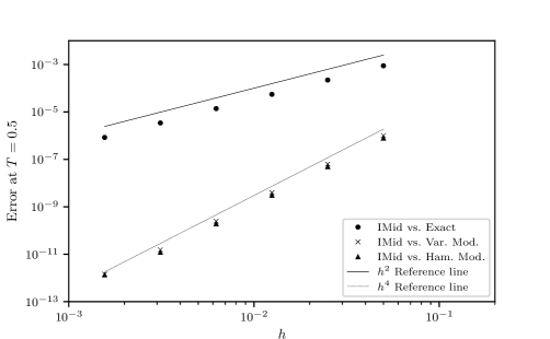
In our numerical example, we take the nonlinearity . Figure 1 shows that both the Hamiltonian and the variational modified system show the expected scaling when compared to the solution of the implicit midpoint rule. (Due to the symmetry of the method only even powers of appear in the modified equations at any order.) The modified equations were solved with a highly resolved standard forth order explicit Runge–Kutta method.
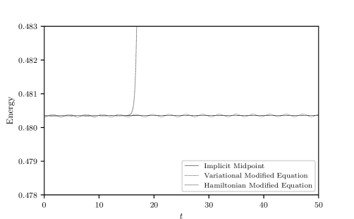
Figure 2 shows the approximate preservation of energy of the implicit midpoint rule and of the two modified systems. The occurrence of high frequencies in the Hamiltonian construction leads to numerical blowup, unless the stepsize used in the explicit Runge–Kutta scheme is adjusted to fit a stricter CFL bound. The graphs display the semilinear wave energy; the respective modified energies would be exactly preserved by the true solutions to the modified equations.
9 Well-posedness of the new modified system
In the following we provide a functional framework which shows that, in the limit of vanishing stepsize , the variational modified system with the choice of parameters as in Section 8 behaves analytically like the original semilinear wave equation. We begin by proving a statement on the operator defined in (51). For convenience, we write with
| (59) |
and
| (60) |
Let denote the Lebesgue space of square integrable functions on the circle, which we endow with norm
| (61) |
the space of essentially bounded functions endowed with the usual essential sup-norm, and the Sobolev space of functions whose generalized derivative of order belongs to , endowed with norm
| (62) |
Lemma 1.
For every there exists such that for every , with , and , the equation has a unique solution and there exists a constant such that
| (63) |
and
| (64) |
Moreover, for fixed and under the above bounds on and , the mapping is uniformly Lipschitz continuous as a map from to .
Proof.
As in (53), we write in fixed point form as
| (65) |
Since , the inverse Helmholtz operator, has norm as an operator from to , there exists a constant such that
| (66) |
Hence, there exists such that for all the map is a contraction, hence has a unique fixed point by the contraction mapping theorem.
Taking the -norm of (65), we obtain
| (67) |
which implies (63). Taking the -norm of (65) and noting that has norm as an operator from into , we find
| (68) |
Now suppose that and . Then
| (69) |
Taking the -norm on both sides, we find that
| (70) |
so that, for some ,
| (71) |
Due to (63), this estimate implies uniform Lipschitz continuity of as a map from into . Then, taking the -norm of (69) and using the operator norm of as a map from to implies uniform Lipschitz continuity into as well. ∎
To proceed, we write to denote the space endowed with the nonuniform norm
| (72) |
Note that the space is the “energy space” which corresponds to the modified Hamiltonian (47) with . We therefore seek local well-posedness in this space.
Theorem 2.
For every there exists and such that for every with and every there exists a unique mild solution to the new modified equation (6) with bounds which remain uniform in .
Proof.
We first observe, as can be checked by direct computation, that
| (73) |
so that the new modified system (52) can be written as a semilinear evolution equation of the form (6) with
| (74) |
and
| (75) |
Let denotes the space of functions with vanishing mean endowed with the norm
| (76) |
The crucial observation is that generates a unitary group on . Moreover,
| (77) |
Taking the -norm of this expression, using the uniform Lipschitz continuity of and estimate (63) as asserted by Lemma 1, and supposing that has an bound of , say, we find that there exists such that for all ,
| (78) |
Noting that
| (79) |
and
| (80) |
uniformly under the assumed bounds on and , we find that
| (81) |
A similar argument, now taking the -norm of (77) and using (64) rather than (63) shows that
| (82) |
This proves uniform Lipschitz continuity of in .
This theorem shows that the new modified equation is well posed in a space which limits to the standard setting for the original semilinear wave equation as . We note that the theorem and proof easily translates up the scale of standard Sobolev spaces.
10 All-order modified equations: the linear case
Let us now consider how the procedure set up in Sections 5 and 6 generalizes to higher orders. We first consider the linear case, which can be treated for all orders at once via a generating function approach. In Section 11 below, we extend this approach to the nonlinear case using an iterative construction that terminates at fixed, but arbitrary order.
We say that modified Lagrangians and are equivalent at order and write
| (83) |
whenever the difference between solutions of Euler-Lagrange equations for and with their respective arguments held fixed at the temporal endpoints is . Two formal power series are equivalent whenever they are equivalent at every finite order .
First, by performing all steps laid out in Section 5 consistently at any order, we find that the general modified Lagrangian for the implicit midpoint rule applied to the linear wave equation reads
| (84) |
where and, for ,
| (85) |
Proceeding formally, we integrate by parts, recognize the resulting power series as cosine series, and finally apply standard trigonometric identities to obtain
| (86) |
where the linear operators and are given by
| (87) |
and stands for the imaginary unit. Let us now make the transformation ansatz
| (88) |
Plugging this ansatz into (86) and noting that and are commuting self-adjoint operators, we have
| (89) |
Thus, a sufficient condition for removing time derivatives of order larger than from the modified Lagrangian is
| (90) |
where and are analytic functions. Solving for , we obtain
| (91) |
Now the task is to (i) find a function , analytic in a neighborhood of the origin, such that is analytic in a neighborhood of the origin and (ii) find a function such that is a small perturbation of the identity in the sense that . We show that the unique choice
| (92) |
fulfills these conditions. The proof is based on the following fact.
Lemma 3.
Let be analytic in a neighborhood of origin. Then the function
| (93) |
is analytic near the origin. Moreover, if is bounded on , the coefficients of the Maclaurin expansion of with respect to are bounded functions of .
Proof.
We compute, changing the order of summation in the last step,
| (94) |
where the Maclaurin coefficients are given by
| (95) |
Hence, is analytic. Moreover, if is bounded on ,
| (96) |
so is also bounded on . ∎
Corollary 4.
Suppose that, in addition, , , has an analytic inverse near the origin, and is nonzero on . Then
| (97) |
is analytic near the origin, , and the coefficients of the Maclaurin expansion of with respect to are bounded functions of on .
Proof.
Analyticity is obvious. To show boundedness of the Maclaurin coefficients of , note that the Maclaurin coefficients of
| (98) |
are finite linear combinations of the Maclaurin coefficients from Lemma 3, hence are bounded. Dividing by and taking the root does not change this conclusion. ∎
Returning back to (92), we see that the stated choice of is necessary to ensure analyticity of in a neighborhood of the origin, as
| (99) |
has a non-removable singularity on the lines unless its numerator vanishes. By Corollary 4, it is also sufficient. The choice of stated in (92) is then necessary to ensure that , i.e., that the transformation is near-identity. By Corollary 4, this choice is also sufficient. Moreover, it guarantees that the coefficients of the Maclaurin expansion of with respect to are bounded functions of .
Inserting the expression for into (91) and using standard trigonometric identities, we conclude that the transformation operator has the generating function
| (100) |
which, when expanded and truncated at any finite order in , has coefficients which are bounded operators in space.
Substituting this choice back into (90) and then into in transformed variables, equation (89), we obtain
| (101) |
so that the linear modified Euler–Lagrange equation, computed to all orders, reads
| (102) |
or, more explicitly,
| (103) |
where is the pseudodifferential operator with symbol
| (104) |
The operator is bounded on with operator norm . Note that this expression reproduces the dispersion relation for the implicit midpoint rule applied to the linear wave equation [4, Section 4.2] exactly.
11 High-order modified equations: the nonlinear case
To construct the modified Lagrangian for the nonlinear system, we follow the procedure in Section 5 to a fixed order . We do not write out the higher-order terms explicitly, but note that they potentially contain multiples of all higher-order terms that appear on the right hand side of a Faà di Bruno expansion of with respect to , i.e., may contain time derivatives up to order . To eliminate time derivatives of second and higher order from the modified Lagrangian, we proceed in two steps. In the first step, we perform the transformation to all orders exactly as outlined in Section 10. In the second step, we remove these higher-order time derivatives from the variational principle iteratively, applying an additional near-identity transformation at each step. The procedure for doing so is motivated by the approach in [14], but is more involved due to the presence of spatial derivatives.
To see how the modified nonlinear term changes under the transformation (100), we expand with respect to and truncate at order . This truncated expansion takes the form
| (105) |
where the are self-adjoint spatial operators that implicitly depend on , but are uniformly bounded on as . In this sense, this series is well-ordered. Inserting the full into the quadratic terms and the expanded into , we obtain that with
| (106) |
as in (101) and, due to the Faà di Bruno formula and up to terms of ,
| (107) |
where denotes a -fold repetition of the argument and the are -linear forms which smoothly depend on and and which are uniformly bounded on as . Due to the uniform boundedness of the , we obtain what is effectively a variational principle for an ODE, albeit with higher-order time derivatives in the nonlinear contributions.
We now proceed to iteratively eliminate the higher time derivatives from (107). To structure the discussion, let
| (108) |
with multilinear forms as described above, denote the vector spaces of functions appearing in the inner sum of (107). On , we have a natural equivalence of elements via integration by parts in time or space under the action integral. We write if the functions give the same contribution to the resulting Euler–Lagrange equations. Note that any is equivalent to
| (109) |
where and depends on and only. Indeed, if any monomial of contains only first or second time derivatives, it is already of the required form. If not, there must be a higher-order time derivatives and we can “peel off” time derivatives by repeated integration by parts until exactly two are left. When , by the same argument, the second term on the right of (109) can always taken to be zero.
Further, let
| (110) |
The first index limits the maximal number of time derivatives contained in each of the monomials of elements of and the second index gives the excess order in at which time derivatives occur. Clearly, if and if and .
We say that two elements from are equivalent if they are agree in the sense of equivalence of the , up to terms of . Note that the entire sum on the right of (107) is contained in . We are now going to apply a sequence of transformations to the effect that, up to equivalences, the resulting Lagrangian density depends only on time derivatives of order one. We will do so by using (109) at each step to split off higher powers of first derivatives from a remainder, remove second time derivative contributions via a suitably chosen transformation, and iterate this process until this remainder is either of class or of class . In both of these terminal cases, the monomials making up the remainder contribution contain at most two time derivatives, which can always be integrated by parts such that only first time derivatives remain.
To simplify language and notation, we will use the same symbols for quantities in old and new variables. Thus, the transformations will be referred to as “replacements,” which is algebraically equivalent. As we implement these replacements, a corresponding concatenation of transformations could be constructed. However, we will not write them down explicitly and only note that these transformation only contain uniformly bounded spatial operators. To begin we note that, up to equivalences, the following relations hold.
-
(i)
If , then .
-
(ii)
If , then .
-
(iii)
If , then .
-
(iv)
If and , then .
-
(v)
If , then the replacement in the expression for corresponds to the replacement for some .
-
(vi)
If and with , then the replacement in the expression for corresponds to the replacement for some .
With these provisions, the modified Lagrangian density, after applying the all-order linear transformation and (109), can be written
| (111) |
where and, by (109), can be chosen to depend only on and with . Now consider the replacement
| (112) |
Then
| (113) |
for some and . Next,
| (114) |
with . Finally, when transforming and higher-order Lagrangian densities that contain no more than first derivatives of , then by (v) and (vi), the additional remainder term is also of class . Thus, altogether, the first elimination step results in the replacement
| (115) |
with , and where and .
Now, for the general case, suppose that we are at a stage where the modified Lagrangian has been transformed into
| (116) |
where, and by (109), can be chosen to depend only on and with . Now consider the replacement
| (117) |
with . Then
| (118) |
for some and . Next,
| (119) |
with . Finally, when transforming and higher-order Lagrangian densities that contain no more than first derivatives of , then by (v) and (vi), the additional remainder term is also of class . Thus, altogether, one elimination step results in the replacement
| (120) |
with .
We iterate this (inner) replacement until , at which point we only two time derivatives are left so that we can always choose such that depends only on and , so that
| (121) |
where depends only on and and . Now consider the (outer) replacement
| (122) |
with . Then
| (123) |
for some and . Next,
| (124) |
with . Finally, when transforming and higher-order Lagrangian densities that contain no more than first derivatives of , then by (v) and (vi), the additional remainder term is also of class . Thus, altogether, one elimination step results in the replacement
| (125) |
where and . We can then eliminate by following the inner replacement loop to its end.
Altogether, we iterate the outer replacement loop until , at which point we can remove all second derivatives and obtain a final -modified Lagrangian density of the form
| (126) |
where depends only on and .
12 Conclusions
Modified equations for backward error analysis of variational integrators can be systematically constructed using a formal Taylor expansion of the action integral. However, a straightforward variational construction necessitates the use of an extended phase space. We have demonstrated for the model case of the implicit midpoint rule applied to the semilinear wave equation that a carefully chosen configuration space transformation allows us to eliminate the dependence of the modified Lagrangian on higher order time derivatives, thus reducing the phase space, and refitting the modified equations into the standard framework of Lagrangian mechanics. Furthermore, such construction yields modified equations whose dynamics lives on timescales that coincide with the timescales of the unmodified partial differential equation. This is clearly not the case for the modified equations derived on the Hamiltonian side using the traditional method as can already be seen when discretizing the linear wave equation.
Even though we looked only at the next-order correction for the implicit midpoint scheme in detail, we have shown that our construction generalizes to any order. We also expect that the computations shown here generalize in a straightforward way to semilinear Hamiltonian evolution equations with a linear part containing a general self-adjoint time-independent operator in place of , provided there is a regular Legendre transform.
Our approach was initially developed in the context of Hamiltonian systems with strong gyroscopic forces [13, 26]; the present work demonstrates that the strategy is more widely applicable and might point toward an abstract theory of degenerate variational asymptotics. We also note that the flexibility of the approach comes from the fact that the variational construction modifies the symplectic structure and the Hamiltonian simultaneously. In contrast, the traditional construction keeps a canonical symplectic structure and only modifies the Hamiltonian.
Two major questions remain open. First, is it possible to show, using the new variational modified equation, that the implicit midpoint rule preserves the energy to fourth order? Note that for the new modified equations, the truncation remainder is for fixed and , while it is unbounded in the traditional setting. Therefore, we expect that we still need some assumptions on the regularity of the solution—even though numerical simulations indicate that energy preservation of the implicit midpoint rule is very good even for non-smooth data—but the regularity conditions are possibly less stringent than those needed in [37]. Second, is it possible to achieve exponential asymptotics as in the standard backward error analysis for ODEs? To answer this question, it is necessary to describe the combinatorics of the new asymptotic series, which should be possible, but is more complicated than the conventional construction.
Acknowledgments
We thank Melvin Leok, Haidar Mohamad, Mats Vermeeren and, in particular, Claudia Wulff for stimulating discussion on the subject of this paper. This work was supported in part by DFG grant OL-155/3-2. This paper is a contribution to project L2 of the Collaborative Research Center TRR 181 “Energy Transfers in Atmosphere and Ocean” funded by the Deutsche Forschungsgemeinschaft (DFG, German Research Foundation) under project number 274762653.
References
- [1] V. I. Arnol’d, Geometrical methods in the theory of ordinary differential equations, Springer-Verlag, New York, second ed., 1988.
- [2] G. Benettin and A. Giorgilli, On the Hamiltonian interpolation of near-to-the-identity symplectic mappings with application to symplectic integration algorithms, J. Statist. Phys., 74 (1994), pp. 1117–1143.
- [3] P. Brenner, M. Crouzeix, and V. Thomée, Single-step methods for inhomogeneous linear differential equations in Banach space, RAIRO Anal. Numér., 16 (1982), pp. 5–26.
- [4] T. J. Bridges and S. Reich, Numerical methods for Hamiltonian PDEs, J. Phys. A, 39 (2006), pp. 5287–5320.
- [5] B. Cano, Conserved quantities of some Hamiltonian wave equations after full discretization, Numer. Math., 103 (2006), pp. 197–223.
- [6] D. Cohen, E. Hairer, and C. Lubich, Conservation of energy, momentum and actions in numerical discretizations of non-linear wave equations, Numer. Math., 110 (2008), pp. 113–143.
- [7] C. J. Cotter and S. Reich, Semigeostrophic particle motion and exponentially accurate normal forms, Multiscale Model. Simul., 5 (2006), pp. 476–496.
- [8] A. Debussche and E. Faou, Modified energy for split-step methods applied to the linear Schrödinger equation, SIAM J. Numer. Anal., 47 (2009), pp. 3705–3719.
- [9] G. Dujardin and E. Faou, Normal form and long time analysis of splitting schemes for the linear Schrödinger equation with small potential, Numer. Math., 108 (2007), pp. 223–262.
- [10] E. Faou, B. Grébert, and E. Paturel, Birkhoff normal form for splitting methods applied to semilinear Hamiltonian PDEs. I. Finite-dimensional discretization, Numer. Math., 114 (2010), pp. 429–458.
- [11] , Birkhoff normal form for splitting methods applied to semilinear Hamiltonian PDEs. II. Abstract splitting, Numer. Math., 114 (2010), pp. 459–490.
- [12] L. Gauckler and C. Lubich, Splitting integrators for nonlinear Schrödinger equations over long times, Found. Comput. Math., 10 (2010), pp. 275–302.
- [13] G. Gottwald, M. Oliver, and N. Tecu, Long-time accuracy for approximate slow manifolds in a finite-dimensional model of balance, J. Nonlinear Sci., 17 (2007), pp. 283–307.
- [14] G. A. Gottwald and M. Oliver, Slow dynamics via degenerate variational asymptotics, Proc. R. Soc. Lond. Ser. A Math. Phys. Eng. Sci., 470 (2014), p. 20140460.
- [15] E. Hairer and C. Lubich, The life-span of backward error analysis for numerical integrators, Numer. Math., 76 (1997), pp. 441–462.
- [16] E. Hairer, C. Lubich, and G. Wanner, Geometric numerical integration, Springer-Verlag, Berlin, second ed., 2006.
- [17] D. Henry, Geometric theory of semilinear parabolic equations, Springer-Verlag, Berlin-New York, 1981.
- [18] A. L. Islas and C. M. Schober, Backward error analysis for multisymplectic discretizations of Hamiltonian PDEs, Math. Comput. Simulation, 69 (2005), pp. 290–303.
- [19] B. Leimkuhler and S. Reich, Simulating Hamiltonian dynamics, Cambridge University Press, Cambridge, 2004.
- [20] M. Leok and T. Shingel, General techniques for constructing variational integrators, Front. Math. China, 7 (2012), pp. 273–303.
- [21] M. Leok and J. Zhang, Discrete Hamiltonian variational integrators, IMA J. Numer. Anal., 31 (2011), pp. 1497–1532.
- [22] J. E. Marsden and M. West, Discrete mechanics and variational integrators, Acta Numer., 10 (2001), pp. 357–514.
- [23] R. I. McLachlan and C. Offen, Backward error analysis for variational discretisations of PDEs, J. Geom. Mech., 14 (2022), pp. 447–471.
- [24] B. Moore and S. Reich, Backward error analysis for multi-symplectic integration methods, Numer. Math., 95 (2003), pp. 625–652.
- [25] A. I. Neĭshtadt, The separation of motions in systems with rapidly rotating phase, J. Appl. Math. Mech., 48 (1984), pp. 133–139.
- [26] M. Oliver, Variational asymptotics for rotating shallow water near geostrophy: a transformational approach, J. Fluid Mech., 551 (2006), pp. 197–234.
- [27] M. Oliver and S. Vasylkevych, Hamiltonian formalism for models of rotating shallow water in semigeostrophic scaling, Discrete Contin. Dyn. Syst., 31 (2011), pp. 827–846.
- [28] M. Oliver, M. West, and C. Wulff, Approximate momentum conservation for spatial semidiscretizations of semilinear wave equations, Numer. Math., 97 (2004), pp. 493–535.
- [29] M. Oliver and C. Wulff, -stable Runge-Kutta methods for semilinear evolution equations, J. Funct. Anal., 263 (2012), pp. 1981–2023.
- [30] , Stability under Galerkin truncation of A-stable Runge-Kutta discretizations in time, Proc. Roy. Soc. Edinburgh Sect. A, 144 (2014), pp. 603–636.
- [31] A. Pazy, Semigroups of linear operators and applications to partial differential equations, Springer-Verlag, New York, 1983.
- [32] S. Reich, Backward error analysis for numerical integrators, SIAM J. Numer. Anal., 36 (1999), pp. 1549–1570.
- [33] M. Vermeeren, Modified equations for variational integrators, Numer. Math., 137 (2017), pp. 1001–1037.
- [34] , Modified equations for variational integrators applied to Lagrangians linear in velocities, J. Geom. Mech., 11 (2019), pp. 1–22.
- [35] A. P. Veselov, Integrable systems with discrete time, and difference operators, Funktsional. Anal. i Prilozhen., 22 (1988), pp. 1–13, 96.
- [36] J. M. Wendlandt and J. E. Marsden, Mechanical integrators derived from a discrete variational principle, Phys. D, 106 (1997), pp. 223–246.
- [37] C. Wulff and M. Oliver, Exponentially accurate Hamiltonian embeddings of symplectic A-stable Runge–Kutta methods for Hamiltonian semilinear evolution equations, Proc. Roy. Soc. Edinburgh Sect. A, 146 (2016), pp. 1265–1301.