Channel-Adaptive Pilot Design for FDD-MIMO Systems Utilizing Gaussian Mixture Models

Abstract

In this work, we propose to utilize Gaussian mixture models (GMMs) to design pilots for downlink (DL) channel estimation in frequency division duplex (FDD) systems. The GMM captures prior information during training that is leveraged to design a codebook of pilot matrices in an initial offline phase. Once shared with the mobile terminal (MT), the GMM is utilized to determine a feedback index at the MT in the online phase. This index selects a pilot matrix from a codebook, eliminating the need for online pilot optimization. The GMM is further used for DL channel estimation at the MT via observation-dependent linear minimum mean square error (LMMSE) filters, parametrized by the GMM. The analytic representation of the GMM allows adaptation to any signal-to-noise ratio (SNR) level and pilot configuration without re-training. With extensive simulations, we demonstrate the superior performance of the proposed GMM-based pilot scheme compared to state-of-the-art approaches.

I Introduction

In multiple-input multiple-output (MIMO) communication systems, obtaining channel state information (CSI) at the base station (BS) needs to occur in regular time intervals. In FDD systems, both the BS and the MT transmit at the same time but on different frequencies, which breaks the reciprocity between the instantaneous uplink (UL) CSI and DL CSI. Consequently, acquiring accurate DL CSI in FDD systems is challenging [1] and thus relies on feedback of the estimated channel from the MT. Therefore, the quality of DL channel estimation is of crucial importance.

In massive MIMO systems, where the BS is typically equipped with a high number of antennas, as many pilots as transmit antennas are required to be sent from the BS to the MT to fully illuminate the channel, i.e., avoiding a systematic error when relying on least squares (LS) DL CSI estimation at the MT. However, the associated pilot overhead for complete channel illumination can be prohibitive [2]. In scenarios with spatial correlation at the BS and the MT, the DL training overhead can be significantly reduced by leveraging statistical knowledge of the channel and the noise [3, 4, 5, 6, 7, 8], e.g., by using Bayesian estimation approaches.

Hence, for DL channel estimation, given a budget of $n_{\mathrm{p}}$ pilots, a common approach to use for channel illumination is transmitting $n_{\mathrm{p}}$ pilots equivalent to the $n_{\mathrm{p}}$ dominant eigenvectors of the transmit-side spatial correlation matrix. However, the aforementioned works rely on either perfect or estimated statistical knowledge at the BS and/or at the MT side, which may be difficult to acquire.

Contributions: In this work, we propose to utilize GMMs for pilot design. The proposed scheme neither requires a priori knowledge of the channel’s statistics at the BS nor the MT. The statistical prior information captured with the GMM in the offline phase is exploited to determine a feedback index at the MT in the online phase utilizing the GMM, which is shared between the BS and the MT. This feedback index is sufficient to establish common knowledge of the pilot matrix, which is selected from a codebook of pilot matrices. Thus, no online pilot optimization is required. The inference of the feedback information involves computing the responsibilities via the GMM and conducting a maximum a posteriori (MAP) estimation, which selects the index of the GMM component with the largest responsibility as the feedback index. The responsibilities determine how well each component of the GMM describes the underlying channel, measured in terms of posterior probabilities. The responsibilities are additionally used to obtain an estimated channel at the MT by performing a convex combination of observation-dependent LMMSE filters, which are parametrized by the GMM and applied to the observation. Moreover, the analytic representation of the GMM generally allows the adaption to any SNR level and pilot configuration without re-training. Based on extensive simulations, we highlight the superior performance of the proposed GMM-based pilot scheme compared to state-of-the-art approaches.

II System and Channel Model

We consider a BS equipped with $N_{\mathrm{tx}}$ antennas and a MT equipped with $N_{\mathrm{rx}}$ antennas. We assume a block-fading model, cf., e.g., [9], where the DL signal for block $t$ received at the MT is expressed as

$$\bm{Y}_{t}=\bm{H}_{t}\bm{P}^{\operatorname{T}}_{t}+\bm{N}_{t}\in\mathbb{C}^{N_{\mathrm{rx}}\times n_{\mathrm{p}}}$$ (1)

where $t=0,\dots,T$, with the MIMO channel $\bm{H}_{t}\in\mathbb{C}^{N_{\mathrm{rx}}\times N_{\mathrm{tx}}}$, the pilot matrix $\bm{P}_{t}\in\mathbb{C}^{n_{\mathrm{p}}\times N_{\mathrm{tx}}}$, and the additive white Gaussian noise (AWGN) $\bm{N}_{t}=[\bm{n}^{\prime}_{t,1},\dots,\bm{n}^{\prime}_{t,n_{\mathrm{p}}}]\in\mathbb{C}^{N_{\mathrm{rx}}\times n_{\mathrm{p}}}$ with $\bm{n}^{\prime}_{t,p}\sim\mathcal{N}_{\mathbb{C}}(\bm{0},\sigma_{n}^{2}\mathbf{I}_{N_{\mathrm{rx}}})$ for $p\in\{1,2,\dots,n_{\mathrm{p}}\}$ and $n_{\mathrm{p}}$ is the number of pilots. We consider systems with reduced pilot overhead, i.e., $n_{\mathrm{p}}<N_{\mathrm{tx}}$. For the subsequent analysis, it is advantageous to vectorize (1):

$$\bm{y}_{t}=(\bm{P}_{t}\otimes\mathbf{I}_{N_{\mathrm{rx}}})\bm{h}_{t}+\bm{n}_{t}$$ (2)

where $\bm{h}_{t}=\operatorname{vec}(\bm{H}_{t})$, $\bm{y}_{t}=\operatorname{vec}(\bm{Y}_{t})$, $\bm{n}_{t}=\operatorname{vec}(\bm{N}_{t})$, and $\bm{n}_{t}\sim\mathcal{N}_{\mathbb{C}}(\mathbf{0},{\bm{\Sigma}})$ with ${\bm{\Sigma}}=\sigma_{n}^{2}\mathbf{I}_{N_{\mathrm{rx}}n_{\mathrm{p}}}$.

We adopt the 3rd Generation Partnership Project (3GPP) spatial channel model (see [10, 9]) where channels are modeled conditionally Gaussian, i.e., $\bm{h}_{t}|{\bm{\delta}}\sim\mathcal{N}_{\mathbb{C}}({\bm{0}},\bm{C}_{{\bm{\delta}}})$. The covariance matrix $\bm{C}_{{\bm{\delta}}}$ is assumed to remain constant over $T+1$ blocks. The random vector ${\bm{\delta}}$ comprises the main angles of arrival/departure of the multi-path propagation cluster between the BS and the MT. The main angles of arrival/departure are drawn independently and are uniformly distributed over $[\frac{-\pi}{2},\frac{\pi}{2}]$. The BS as well as the MT employ a uniform linear array (ULA) such that the transmit- and receive-side spatial channel covariance matrices are given by

$$\bm{C}_{{\bm{\delta}}}^{\mathrm{\{rx,tx\}}}=\int_{-\pi}^{\pi}g^{\mathrm{\{rx,tx\}}}(\theta;{\bm{\delta}})\bm{a}^{\mathrm{\{rx,tx\}}}(\theta)\bm{a}^{\mathrm{\{rx,tx\}}}(\theta)^{\operatorname{H}}d\theta,$$ (3)

where $\bm{a}^{\mathrm{\{rx,tx\}}}(\theta)=[1,e^{j\pi\sin(\theta)},\dots,e^{j\pi(N_{\mathrm{\{rx,tx\}}}-1)\sin(\theta)}]^{\operatorname{T}}$ is the array steering vector for an angle of arrival/departure $\theta$ and $g^{\mathrm{\{rx,tx\}}}$ is a Laplacian power density whose standard deviation describes the angular spread $\sigma_{\text{AS}}^{\mathrm{\{rx,tx\}}}$ of the propagation cluster at the BS ($\sigma_{\text{AS}}^{\mathrm{tx}}=$2\text{\,}\mathrm{\SIUnitSymbolDegree}$$) and MT ($\sigma_{\text{AS}}^{\mathrm{rx}}=$35\text{\,}\mathrm{\SIUnitSymbolDegree}$$) side [10]. The overall channel covariance matrix is constructed as $\bm{C}_{{\bm{\delta}}}=\bm{C}_{{\bm{\delta}}}^{\mathrm{tx}}\otimes\bm{C}_{{\bm{\delta}}}^{\mathrm{rx}}$ due to the assumption of independent scattering in the vicinity of transmitter and receiver, see, e.g., [11]. In the case of a MT equipped with a single antenna, $\bm{C}_{{\bm{\delta}}}$ degenerates to the transmit-side covariance matrix $\bm{C}_{{\bm{\delta}}}^{\mathrm{tx}}$.

With

$$\mathcal{H}=\{\bm{h}^{\ell}\}_{\ell=1}^{L},$$ (4)

we denote the training data set consisting of $L$ channel samples. For every channel sample $\bm{h}^{\ell}$, we generate random angles, collected in ${\bm{\delta}}^{\ell}$, and then draw the sample as $\bm{h}^{\ell}\sim\mathcal{N}_{\mathbb{C}}({\bm{0}},\bm{C}_{{\bm{\delta}}^{\ell}})$. These channels represent a communications environment with unknown probability density function (PDF) $f_{\bm{h}}$.

III Pilot Optimization with Perfect Statistical Knowledge

Given the knowledge of ${\bm{\delta}}$, the observation $\bm{y}_{t}$ is jointly Gaussian with the channel $\bm{h}_{t}$ [see (2)], and we can compute a genie LMMSE channel estimate with [9]

$$\hat{\bm{h}}_{t,\text{gLMMSE}}=\operatorname{E}[\bm{h}_{t}\mid\bm{y}_{t},{\bm{\delta}}]$$ (5)

$$=\bm{C}_{{\bm{\delta}}}(\bm{P}_{t}\otimes\mathbf{I}_{N_{\mathrm{rx}}})^{\operatorname{H}}((\bm{P}_{t}\otimes\mathbf{I}_{N_{\mathrm{rx}}})\bm{C}_{{\bm{\delta}}}(\bm{P}_{t}\otimes\mathbf{I}_{N_{\mathrm{rx}}})^{\operatorname{H}}+{\bm{\Sigma}})^{-1}\bm{y}_{t}.$$ (6)

The goal of pilot optimization is to design the pilot matrix $\bm{P}_{t}$ such that the mean squared error (MSE) between $\hat{\bm{h}}_{t,\text{gLMMSE}}$ and the actual channel $\bm{h}_{t}$ is minimized [7, 6, 3]:

$$\bm{P}_{t}^{\star}=\operatorname*{arg\,min}_{\bm{P}_{t}}\ \operatorname{E}[\|\hat{\bm{h}}_{t,\text{gLMMSE}}-\bm{h}_{t}\|_{2}^{2}]$$ (7)

where the pilot matrix $\bm{P}_{t}$ typically satisfies either a total power constraint as in [7, 6] or an equal power per pilot vector constraint as in [3]. In this work, we will consider the latter case. For a given ${\bm{\delta}}$, the optimal pilot matrix $\bm{P}_{t}^{\star}$ for every block is the same, i.e., $\bm{P}^{\star}_{t}=\bm{P}_{\text{genie}}$ for all $t=0,\dots,T$. In particular, $\bm{P}_{\text{genie}}$ is a sub-unitary matrix [3]

$$\bm{P}_{\text{genie}}=\sqrt{\rho}\bm{U}_{\bm{\delta}}^{\operatorname{H}}[:n_{\mathrm{p}},:],$$ (8)

which is composed of the $n_{\mathrm{p}}$ dominant eigenvectors of the transmit-side covariance matrix $\bm{C}_{{\bm{\delta}}}^{\mathrm{tx}}=\bm{U}_{\bm{\delta}}\bm{\Lambda}_{\bm{\delta}}\bm{U}_{\bm{\delta}}^{\operatorname{H}}$ corresponding to the $n_{\mathrm{p}}$ largest eigenvalues, where $\rho$ denotes the transmit power per pilot vector. Note that power loading across pilot vectors generally achieves better performance but requires additional processing. Additionally, with a sub-unitary pilot design, our proposed scheme yields a codebook consisting of pilot matrices that do not depend on the SNR, resolving the burden of saving SNR level-specific pilot codebooks, see Subsection IV-D.

IV GMM-based Pilot Design and Downlink Channel Estimation

Any channel $\bm{h}_{t}$ of a MT located anywhere within the BS’s coverage area can be interpreted as a realization of a random variable with PDF $f_{\bm{h}}$ for which however, no analytical expression is available. Therefore, we utilize a GMM to approximate the PDF $f_{\bm{h}}$, similar to [12, 13]. This learned model is then shared between the BS and the MT to establish common awareness of the channel characteristics. The GMM is then utilized to infer feedback information for pilot matrix design and for DL channel estimation at the MT in the online phase. Thereby, the feedback information of the MT of a preceding fading block $t-1$ is leveraged at the BS to select the pilot matrix for the subsequent fading block $t>0$.

IV-A Modeling the Channel Characteristics at the BS – Offline

The channel characteristics are captured offline using a GMM comprised of $K=2^{B}$ components,

$$f^{(K)}_{\bm{h}}(\bm{h}_{t})=\sum\nolimits_{k=1}^{K}\pi_{k}\mathcal{N}_{\mathbb{C}}(\bm{h}_{t};{\bm{\mu}}_{k},\bm{C}_{k})$$ (9)

where each component of the GMM is defined by the mixing coefficient $\pi_{k}$, the mean ${\bm{\mu}}_{k}$, and the covariance matrix $\bm{C}_{k}$.

Motivated by the observation that the channel exhibits an unconditioned zero mean and similar to [14], we enforce the means of the GMM-components to zero, i.e., ${\bm{\mu}}_{k}=\bm{0}$ for all $k\in\{1,\dots,K\}$. This also reduces the number of learnable parameters and, thus, prevents overfitting. Note that the parameters of the GMM, i.e., $\{\pi_{k},\bm{C}_{k}\}_{k=1}^{K}$, remain constant across all blocks. To obtain maximum likelihood estimates of the GMM parameters, we utilize the training dataset $\mathcal{H}$ [see (4)] and employ an expectation maximization (EM) algorithm, as described in [15, Subsec. 9.2.2], where we enforce the means to zero in every M-step of the EM algorithm.

For MIMO channels, we further impose a Kronecker factorization on the covariances of the GMM, i.e., $\bm{C}_{k}=\bm{C}^{\mathrm{tx}}_{k}\otimes\bm{C}^{\mathrm{rx}}_{k}$. Thus, instead of fitting an unconstrained GMM with $N\times N$-dimensional covariances (where $N=N_{\mathrm{tx}}N_{\mathrm{rx}}$), we fit separate GMMs for the transmit and receive sides. These transmit-side and receive-side GMMs possess $N_{\mathrm{tx}}\times N_{\mathrm{tx}}$ and $N_{\mathrm{rx}}\times N_{\mathrm{rx}}$-dimensional covariances, respectively, with $K_{\mathrm{tx}}$ and $K_{\mathrm{rx}}$ components. Then, by computing the Kronecker products of the corresponding transmit-side and receive-side covariance matrices, we obtain a GMM with $K=K_{\mathrm{tx}}K_{\mathrm{rx}}$ components and $N\times N$-dimensional covariances. Imposing this constraint on the GMM covariances not only significantly decreases the duration of offline training, facilitates parallelization of the fitting process, and demands fewer training samples due to the reduced number of parameters to be learned, cf. [13, 12], but also ensures access to a transmit-side covariance during pilot design in the online phase, as discussed in Subsection IV-D.

Using a GMM, we can calculate the posterior probability that the channel $\bm{h}_{t}$ originates from component $k$ as [15, Sec. 9.2],

$$p(k\mid\bm{h}_{t})=\frac{\pi_{k}\mathcal{N}_{\mathbb{C}}(\bm{h}_{t};\bm{0},\bm{C}_{k})}{\sum_{i=1}^{K}\pi_{i}\mathcal{N}_{\mathbb{C}}(\bm{h}_{t};\bm{0},\bm{C}_{i})}.$$ (10)

These posterior probabilities are commonly referred to as responsibilities.

IV-B Sharing the Model with the MTs – Offline

For a MT to infer the feedback information, it must have access to the parameters of the GMM. Conceptually, this involves sharing the model parameters, i.e., $\{\pi_{k},\bm{C}_{k}\}_{k=1}^{K}$, with the MTs upon entering the coverage area of the BS. This transfer is required only once since the GMM remains unchanged for a specific BS environment.

Incorporating model-based insights to restrict the GMM covariances, as discussed in Subsection IV-A, additionally significantly reduces the model transfer overhead. Due to specific antenna array geometries, the GMM covariances can be further constrained to a Toeplitz or block-Toeplitz matrix with Toeplitz blocks, in case of a ULA or uniform rectangular array (URA), respectively, cf. [16], with even fewer parameters. In [16], it is also further discussed how GMMs with variable bit lengths can be obtained. These further structural constraints, as well as the analysis with variable bit lengths, are out of the scope of this work.

IV-C Inferring the Feedback Information and Estimating the Channel at the MTs – Online

In the online phase, the MT infers feedback information given the observation $\bm{y}_{t}$ utilizing the GMM. The joint Gaussian nature of each GMM component [see (9)] combined with the AWGN, allows for simple computation of the GMM of the observations with the GMM from (9) as

$$\small f_{\bm{y}}^{(K)}(\bm{y}_{t})=\sum\nolimits_{k=1}^{K}\pi_{k}\mathcal{N}_{\mathbb{C}}(\bm{y}_{t};\bm{0},(\bm{P}_{t}\otimes\mathbf{I}_{N_{\mathrm{rx}}})\bm{C}_{k}(\bm{P}_{t}\otimes\mathbf{I}_{N_{\mathrm{rx}}})^{\operatorname{H}}+{\bm{\Sigma}}).$$ (11)

Thus, the MT can compute the responsibilities based on the observations $\bm{y}_{t}$ as

$$\small p(k\mid\bm{y}_{t})=\frac{\pi_{k}\mathcal{N}_{\mathbb{C}}(\bm{y}_{t};\bm{0},(\bm{P}_{t}\otimes\mathbf{I}_{N_{\mathrm{rx}}})\bm{C}_{k}(\bm{P}_{t}\otimes\mathbf{I}_{N_{\mathrm{rx}}})^{\operatorname{H}}+{\bm{\Sigma}})}{\sum_{i=1}^{K}\pi_{i}\mathcal{N}_{\mathbb{C}}(\bm{y}_{t};\bm{0},(\bm{P}_{t}\otimes\mathbf{I}_{N_{\mathrm{rx}}})\bm{C}_{i}(\bm{P}_{t}\otimes\mathbf{I}_{N_{\mathrm{rx}}})^{\operatorname{H}}+{\bm{\Sigma}})}.$$ (12)

The feedback information $k_{t}^{\star}$ is then determined through a MAP estimation as

$$k^{\star}_{t}=\operatorname*{arg\,max}_{k}~{}{p(k\mid\bm{y}_{t})}$$ (13)

where the index of the component with the highest responsibility for the observation $\bm{y}_{t}$ serves as the corresponding feedback information. The responsibilities measure how well each component of the GMM explains the underlying channel $\bm{h}_{t}$ of the observed pilot signal $\bm{y}_{t}$. Hence, the feedback information is simply the index of the GMM component that best explains the underlying channel. Subsequently, the responsibilities are utilized to obtain a channel estimate via the GMM by calculating a convex combination of per-component LMMSE estimates, as discussed in [13, 12]. In particular, the MT estimates the channel by computing

$$\hat{\bm{h}}_{t,\text{GMM}}(\bm{y})=\sum_{k=1}^{K}p(k\mid\bm{y}_{t})\hat{\bm{h}}_{t,\text{LMMSE},k}(\bm{y}_{t}),$$ (14)

using the responsibilities $p(k\mid\bm{y}_{t})$ from (12) and

$$\hat{\bm{h}}_{t,\text{LMMSE},k}(\bm{y}_{t})$$

$$=\bm{C}_{k}(\bm{P}_{t}\otimes\mathbf{I}_{N_{\mathrm{rx}}})^{\operatorname{H}}((\bm{P}_{t}\otimes\mathbf{I}_{N_{\mathrm{rx}}})\bm{C}_{k}(\bm{P}_{t}\otimes\mathbf{I}_{N_{\mathrm{rx}}})^{\operatorname{H}}+{\bm{\Sigma}})^{-1}\bm{y}_{t}.$$ (15)

IV-D Designing the Pilots at the BS– Online

Consider the eigenvalue decomposition of each of the GMM’s transmit-side covariances, i.e., $\bm{C}_{k}^{\mathrm{tx}}=\bm{U}_{k}\bm{\Lambda}_{k}\bm{U}^{\operatorname{H}}_{k}$. For $t>0$, given the feedback information $k_{t-1}^{\star}$ of the MT from the preceding block $t-1$, we propose employing the pilot matrix $\bm{P}_{t}$ at the BS for the subsequent block $t$ as [cf. (8)]

$$\bm{P}_{t}=\sqrt{\rho}\bm{U}^{\operatorname{H}}_{k^{\star}_{t-1}}[:n_{\mathrm{p}},:],$$ (16)

i.e., the $n_{\mathrm{p}}$ dominant eigenvectors of the $k^{\star}_{t-1}$-th transmit-side covariance matrix $\bm{C}_{k^{\star}_{t-1}}^{\mathrm{tx}}$ are selected as the pilot matrix. Since the GMM-covariances remain fixed, we can store a set of pilot matrices $\mathcal{P}=\{\bm{U}^{\operatorname{H}}_{k}[:n_{\mathrm{p}},:]\}_{k=1}^{K}$, and the online pilot design utilizing the proposed GMM-based scheme simplifies to a simple selection task based on the feedback information $k^{\star}_{t-1}$ from the previous block. For the initial block $t=0$, we employ a discrete Fourier transform (DFT)-based pilot matrix.

IV-E Complexity Analysis

The online computational complexity of the proposed GMM-based scheme can be divided into three parts: the inference of the feedback information, the channel estimation, and the pilot design.

Matrix-vector multiplications dominate the computational complexity for inferring the feedback information. This is because the computation of the responsibilities in (12) entails evaluating Gaussian densities, and the calculations involving determinants and inverses can be pre-computed for a specific SNR level due to the fixed GMM parameters. Thus, the inference of the feedback information using (13) in the online phase at the MT has a complexity of $\mathcal{O}(KN_{\mathrm{rx}}^{2}n_{\mathrm{p}}^{2})$.

The additional processing to calculate an estimated channel with the GMM via (14) further involves the application of the per-component LMMSE filters [see (IV-C)] which exhibits a computational complexity of $\mathcal{O}(KN_{\mathrm{rx}}^{2}N_{\mathrm{tx}}n_{\mathrm{p}})$, since also the LMMSE filters for a given SNR level can be pre-computed. For the feedback inference and application of the LMMSE filters, parallelization concerning the number of components $K$ is possible.

The computational complexity of the online pilot design is $\mathcal{O}(K)$, as it only involves traversing the pre-computed set of pilot matrices $\mathcal{P}$. Thus, in the online phase, our scheme avoids computing an eigenvalue decomposition, which is required for solving the optimization problem from (8).

V Baseline Channel Estimators and Pilot Schemes

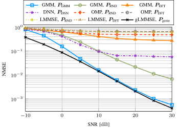
Figure 1: The NMSE over the SNR for a MIMO system ($N_{\mathrm{tx}}=16$, $N_{\mathrm{rx}}=4$) with $B=7$ feedback bits and $n_{\mathrm{p}}=4$ pilots.

In addition to the utopian genie LMMSE approach (5), where we assume perfect knowledge of ${\bm{\delta}}$ (at the BS to design the optimal pilots and at the MT to apply the genie LMMSE estimator), we consider following channel estimators and pilot matrices.

Firstly, we consider the LMMSE estimator $\hat{\bm{h}}_{\text{LMMSE}}$, where the sample covariance matrix is formed using the set $\mathcal{H}$ [see (4)], as discussed in, e.g., [13, 12].

As another baseline, we consider a compressive sensing estimation method $\hat{\bm{h}}_{\text{OMP}}$ employing the orthogonal matching pursuit (OMP) algorithm, cf. [13, 17].

Additionally, we compare to an end-to-end deep neural network (DNN) approach for DL channel estimation with a jointly learned pilot matrix $\bm{P}_{\text{DNN}}$, similar to [18]. To determine the hyperparameters of the DNN, we utilize random search [19], with the MSE serving as the loss function. The DNN architecture comprises $D_{\text{CM}}$ convolutional modules, each consisting of a convolutional layer, batch normalization, and an activation function, where $D_{\text{CM}}$ is randomly selected within $[3,9]$. Each convolutional layer contains $D_{\text{K}}$ kernels, where $D_{\text{K}}$ is randomly selected within $[32,64]$. The activation function in each convolutional module is the same and is randomly selected from $\{\text{ReLu, sigmoid, PReLU, Leaky ReLU, tanh, swish}\}$. Following a subsequent two-dimensional max-pooling, the features are flattened, and a fully connected layer is employed with an output dimension of $2N_{\mathrm{tx}}N_{\mathrm{rx}}$ (concatenated real and imaginary parts of the estimated channel). We train a distinct DNN for each pilot configuration and SNR level, running $50$ random searches per pilot configuration and SNR level and selecting the best-performing DNN for each setup.

Lastly, as further baseline pilot matrices, we utilize a DFT sub-matrix $\bm{P}_{\text{DFT}}$ as the pilot matrix, see, e.g., [20], and alternatively, we consider random pilot matrices denoted by $\bm{P}_{\text{RND}}$, see, e.g., [7].

VI Simulation Results

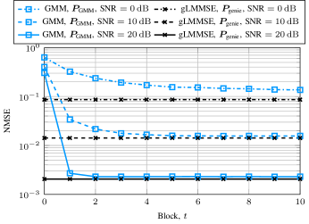
Figure 2: The NMSE over the block index $t$ for a MIMO system ($N_{\mathrm{tx}}=16$, $N_{\mathrm{rx}}=4$) with $B=7$ feedback bits, $n_{\mathrm{p}}=4$ pilots, and $\text{SNR}\in\{$0\text{\,}\mathrm{d}\mathrm{B}$,$10\text{\,}\mathrm{d}\mathrm{B}$,$20\text{\,}\mathrm{d}\mathrm{B}$\}$.

We use the set $\mathcal{H}$ [see (4)] with $L=10^{5}$ samples for fitting the GMM and all other data-based baselines. We use a different dataset of $J=10^{4}$ channel samples per block $t$ for evaluation purposes, where we set $T=10$. The data samples are normalized to satisfy $\operatorname{E}[\|\bm{h}\|^{2}]=N=N_{\mathrm{tx}}N_{\mathrm{rx}}$. Additionally, we fix $\rho=1$, enabling the definition of the SNR as $\frac{1}{\sigma_{n}^{2}}$. We employ the normalized mean squared error (NMSE) as the performance measure. Specifically, for every block $t$, we compute a corresponding channel estimate $\hat{\bm{h}}^{j}$ for each test channel in the set $\{\bm{h}^{j}\}_{j=1}^{J}$, and calculate $\text{NMSE}=\frac{1}{NJ}\sum_{j=1}^{J}\|\bm{h}^{j}-\hat{\bm{h}}^{j}\|^{2}.$ If not mentioned otherwise, we consider the block with index $t=5$ in the subsequent simulations.

In Fig. 1, we simulate a system with $N_{\mathrm{tx}}=16$ BS antennas, $N_{\mathrm{rx}}=4$ MT antennas, and $n_{\mathrm{p}}=4$ pilots. Since we have a MIMO setup, we fit a Kronecker structured GMM with in total $K=2^{7}=128$ components ($B=7$ feedback bits), where $K_{\mathrm{tx}}=32$ and $K_{\mathrm{rx}}=4$. The proposed GMM-based pilot design scheme denoted by “GMM, $\bm{P}_{\text{GMM}}$” outperforms all baselines “{GMM, OMP, LMMSE}, {$\bm{P}_{\text{DFT}}$, $\bm{P}_{\text{RND}}$}” by a large margin, where the GMM estimator, the OMP-based estimator, or the LMMSE estimator, are used in combination with either DFT-based pilot matrices or random pilot matrices. The proposed scheme also outperforms the DNN based approach denoted by “DNN, $\bm{P}_{\text{DNN}}$,” which jointly learns the estimator and a global pilot matrix for the whole scenario; thus, it cannot provide an MT adaptive pilot matrix. This highlights the advantage of the proposed model-based technique over the end-to-end learning technique, which is even trained for each SNR level and pilot configuration. Furthermore, we can observe that the GMM-based pilot design scheme performs only slightly worse than the baseline with perfect statistical information at the BS and MTsee (5) and (8), denoted by “gLMMSE, $\bm{P}_{\text{genie}}$”, being a utopian estimation approach. We can observe a larger gap in the low SNR regime, where the feedback information obtained through the responsibilities given an observation (see (13)) is less accurate due to high noise.

In Fig. 2, we analyze the performance of the GMM-based pilot design scheme depending on the number of blocks $t$ for the same setup as before at three different SNR levels, i.e., $\text{SNR}\in\{$0\text{\,}\mathrm{d}\mathrm{B}$,$10\text{\,}\mathrm{d}\mathrm{B}$,$20\text{\,}\mathrm{d}\mathrm{B}$\}$. As discussed in Subsection IV-D, at $t=0$, we utilize DFT-based pilots. After only one block, we can see a significant gain in performance of the proposed GMM-based pilot design scheme due to the feedback of the index. The results further reveal that with an increasing SNR, fewer blocks are required to achieve a performance close to the utopian baseline “gLMMSE, $\bm{P}_{\text{genie}}$” which requires perfect statistical knowledge at the BS and the MT.

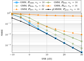
Figure 3: The NMSE over the SNR for a MISO system ($N_{\mathrm{tx}}=64$, $N_{\mathrm{rx}}=1$) with $B=6$ feedback bits and $n_{\mathrm{p}}\in\{16,32,48\}$ pilots.

In the remainder, we consider a multiple-input single-output (MISO) system with $N_{\mathrm{tx}}=64$ BS antennas and $N_{\mathrm{rx}}=1$ antenna at the MT. In Fig. 3 we utilize a GMM with $K=2^{6}=64$ components ($B=6$ feedback bits) and consider setups with $n_{\mathrm{p}}\in\{16,32,48\}$ pilots. In this case, the proposed scheme “GMM, $\bm{P}_{\text{GMM}}$, $n_{\mathrm{p}}=16$”, performs only slightly worse than the genie-aided approach “gLMMSE, $\bm{P}_{\text{genie}}$”. Moreover, the GMM-based pilot design scheme outperforms the baselines “GMM, {$\bm{P}_{\text{DFT}}$, $\bm{P}_{\text{RND}}$}, $n_{\mathrm{p}}\in\{16,32,48\}$”. In particular, the proposed scheme with only $n_{\mathrm{p}}=16$ pilots outperforms random pilot matrices with twice as much pilots ($n_{\mathrm{p}}=32$) or in case of DFT-based pilots even thrice as much pilots ($n_{\mathrm{p}}=48$).

Lastly, in Fig. 4, we analyze the effect of varying the number of GMM-components $K$, on the scheme’s performance, where we set $n_{\mathrm{p}}=16$ and consider three different SNR levels, i.e., $\text{SNR}\in\{$0\text{\,}\mathrm{d}\mathrm{B}$,$10\text{\,}\mathrm{d}\mathrm{B}$,$20\text{\,}\mathrm{d}\mathrm{B}$\}$. We can observe that the estimation error decreases with an increasing number of components $K$. Moreover, with an increasing SNR, the gap to the genie-aided approach “gLMMSE, $\bm{P}_{\text{genie}}$” decreases. Above $K=32$ components, a saturation can be observed. Overall, these results suggest that by varying the number of GMM components $K$, a performance-to-complexity trade-off can be realized without sacrificing too much in performance for $K\geq 16$ components.

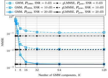
Figure 4: The NMSE over the number of components $K=2^{B}$ for a MISO system ($N_{\mathrm{tx}}=64$, $N_{\mathrm{rx}}=1$) with $n_{\mathrm{p}}=16$ pilots, and $\text{SNR}\in\{$0\text{\,}\mathrm{d}\mathrm{B}$,$10\text{\,}\mathrm{d}\mathrm{B}$,$20\text{\,}\mathrm{d}\mathrm{B}$\}$.

VII Conclusion

In this work, we proposed to utilize GMMs for pilot design in FDD-MIMO systems. A significant advantage of the proposed scheme is that it does not require a priori knowledge of the channel’s statistics at the BS and the MT. Instead, it relies on a feedback mechanism, establishing common knowledge of the pilot matrix. The same GMM can be utilized for DL channel estimation and can be generally adapted to any desired SNR level and pilot configuration without requiring re-training. Simulation results show that the performance gains achieved with the proposed scheme allow the deployment of system setups with reduced pilot overhead while maintaining a similar estimation performance. In our future work, we will investigate the extension of the proposed GMM-based pilot scheme to multi-user systems, see, e.g., [7, 8, 21, 22].

References

- [1] E. Björnson, L. Sanguinetti, H. Wymeersch, J. Hoydis, and T. L. Marzetta, “Massive MIMO is a reality–What is next? five promising research directions for antenna arrays,” Digit. Signal Process., vol. 94, pp. 3 – 20, 2019, Special Issue on Source Localization in Massive MIMO.
- [2] E. Björnson, E. G. Larsson, and T. L. Marzetta, “Massive MIMO: ten myths and one critical question,” IEEE Commun. Mag., vol. 54, no. 2, pp. 114–123, 2016.
- [3] J. Choi, D. J. Love, and P. Bidigare, “Downlink training techniques for FDD massive MIMO systems: Open-loop and closed-loop training with memory,” IEEE J. Sel. Areas Commun., vol. 8, no. 5, pp. 802–814, 2014.
- [4] J. Kotecha and A. Sayeed, “Transmit signal design for optimal estimation of correlated MIMO channels,” IEEE Trans. Signal Process., vol. 52, no. 2, pp. 546–557, 2004.
- [5] E. Björnson and B. Ottersten, “A framework for training-based estimation in arbitrarily correlated Rician MIMO channels with Rician disturbance,” IEEE Trans. Signal Process., vol. 58, no. 3, pp. 1807–1820, 2010.
- [6] J. Pang, J. Li, L. Zhao, and Z. Lu, “Optimal training sequences for MIMO channel estimation with spatial correlation,” in IEEE 66th Veh. Technol. Conf., 2007, pp. 651–655.
- [7] J. Fang, X. Li, H. Li, and F. Gao, “Low-rank covariance-assisted downlink training and channel estimation for FDD massive MIMO systems,” IEEE Trans. Wireless Commun., vol. 16, no. 3, pp. 1935–1947, 2017.
- [8] Y. Gu and Y. D. Zhang, “Information-theoretic pilot design for downlink channel estimation in FDD massive MIMO systems,” IEEE Trans. Signal Process., vol. 67, no. 9, pp. 2334–2346, 2019.
- [9] D. Neumann, T. Wiese, and W. Utschick, “Learning the MMSE channel estimator,” IEEE Trans. Signal Process., vol. 66, no. 11, pp. 2905–2917, Jun. 2018.
- [10] 3GPP, “Spatial channel model for multiple input multiple output (MIMO) simulations,” 3rd Generation Partnership Project (3GPP), Tech. Rep. 25.996 (V16.0.0), Jul. 2020.
- [11] J. Kermoal, L. Schumacher, K. Pedersen, P. Mogensen, and F. Frederiksen, “A stochastic MIMO radio channel model with experimental validation,” IEEE J. Sel. Areas Commun., vol. 20, no. 6, pp. 1211–1226, 2002.
- [12] M. Koller, B. Fesl, N. Turan, and W. Utschick, “An asymptotically MSE-optimal estimator based on Gaussian mixture models,” IEEE Trans. Signal Process., vol. 70, pp. 4109–4123, 2022.
- [13] N. Turan, B. Fesl, M. Koller, M. Joham, and W. Utschick, “A versatile low-complexity feedback scheme for FDD systems via generative modeling,” IEEE Trans. Wireless Commun., early access, Nov. 14, 2023, doi: 10.1109/TWC.2023.3330902.
- [14] B. Fesl, N. Turan, B. Böck, and W. Utschick, “Channel estimation for quantized systems based on conditionally Gaussian latent models,” IEEE Trans. Signal Process., early access, Feb. 29, 2024, doi: 10.1109/TSP.2024.3371872.
- [15] C. M. Bishop, Pattern Recognition and Machine Learning (Information Science and Statistics). Berlin, Heidelberg: Springer-Verlag, 2006.
- [16] N. Turan, B. Fesl, and W. Utschick, “Enhanced low-complexity FDD system feedback with variable bit lengths via generative modeling,” in 57th Asilomar Conf. Signals, Syst., Comput., 2023, to be published, arXiv preprint: 2305.03427.
- [17] A. Alkhateeb, G. Leus, and R. W. Heath, “Compressed sensing based multi-user millimeter wave systems: How many measurements are needed?” in IEEE Int. Conf. Acoust., Speech Signal Process. (ICASSP), 2015, pp. 2909–2913.
- [18] M. B. Mashhadi and D. Gündüz, “Pruning the pilots: Deep learning-based pilot design and channel estimation for MIMO-OFDM systems,” IEEE Trans. Wireless Commun., vol. 20, no. 10, pp. 6315–6328, 2021.
- [19] J. Bergstra and Y. Bengio, “Random search for hyper-parameter optimization,” J. of Mach. Learn. Res., vol. 13, no. null, p. 281–305, Feb. 2012.
- [20] Y. Tsai, L. Zheng, and X. Wang, “Millimeter-wave beamformed full-dimensional MIMO channel estimation based on atomic norm minimization,” IEEE Trans. Commun., vol. 66, no. 12, pp. 6150–6163, 2018.
- [21] Z. Jiang, A. F. Molisch, G. Caire, and Z. Niu, “Achievable rates of FDD massive MIMO systems with spatial channel correlation,” IEEE Trans. Wireless Commun., vol. 14, no. 5, pp. 2868–2882, 2015.
- [22] S. Bazzi and W. Xu, “Downlink training sequence design for FDD multiuser massive MIMO systems,” IEEE Trans. Signal Process., vol. 65, no. 18, pp. 4732–4744, 2017.