Enhancing Privacy in Federated Learning
through Local Training

Abstract

In this paper we propose the federated private local training algorithm (Fed-PLT) for federated learning, to overcome the challenges of (i) expensive communications and (ii) privacy preservation. We address (i) by allowing for both partial participation and local training, which significantly reduce the number of communication rounds between the central coordinator and computing agents. The algorithm matches the state of the art in the sense that the use of local training demonstrably does not impact accuracy. Additionally, agents have the flexibility to choose from various local training solvers, such as (stochastic) gradient descent and accelerated gradient descent. Further, we investigate how employing local training can enhance privacy, addressing point (ii). In particular, we derive differential privacy bounds and highlight their dependence on the number of local training epochs. We assess the effectiveness of the proposed algorithm by comparing it to alternative techniques, considering both theoretical analysis and numerical results from a classification task.

I Introduction

Federated learning has proved to be a powerful framework to enable private cooperative learning [1, 2, 3]. Indeed, federated learning allows a set of agents to pool their resources together to train a more accurate model than any single agent could. This is accomplished by relying on a central coordinator that iteratively collects and aggregates locally trained models – without the need to share raw data. Federated learning has been successfully deployed in different applications, including healthcare [4], wireless networks [5], mobile devices, Internet-of-Things, and sensor networks [6], power systems [7], and intelligent transportation [8], to name a few.

Clearly, all these applications may involve potentially sensitive and/or proprietary training data. Therefore, a fundamental challenge in the federated set-up is to guarantee the privacy of these data throughout the learning process. However, despite the fact that in a federated architecture the agents are not required to share raw data, various attacks have emerged to extract private information from the trained model or its predictions [9, 10, 11]. Thus, employing the federated learning architecture is not sufficient to ensure privacy, and tailored techniques need to be developed [12].

Besides privacy preservation, another fundamental challenge in federated learning is the expensiveness of communications. Indeed, the models exchanged by the agents are oftentimes high dimensional, especially when training (deep) neural networks [3], resulting in resource-intensive communications. Thus, one of the most important objectives is to design federated learning algorithms that employ as few communications as possible, while still guaranteeing good accuracy of the trained model. Different heuristics have been proposed to accomplish this objective, with the main ones arguably being partial participation [13], local training [14], and quantization/compression [15]. In this paper we will focus on the former two, which we review in the following.

As the name suggests, when applying partial participation only a subset of the agents is selected at each iteration to communicate their local models to the coordinator. This allows to reduce the number of agent-coordinator communications required, at the cost of potentially slower convergence [13]. Local training proposes a complementary approach, by aiming to increase the time between communication rounds. The idea is for the agents to perform multiple epochs of local training (e.g. via stochastic gradient descent) for each round of communication. However, this may result in worse accuracy, especially due to the client drift phenomenon [14]. Indeed, locally trained models may be biased by the use of data that are not representative of the overall distribution, thus leading to a drift that cannot be corrected by the coordinator. In this paper we will therefore focus on designing a federated learning algorithm that allows for both partial participation and local training – without compromising accuracy.

Summarizing the discussion above, the objective of this paper is two-fold. On the one hand, we are interested in designing a privacy-preserving federated learning algorithm. On the other hand, we require that such algorithm employs partial participation and local training to reduce the number of communications, but without affecting accuracy. The approach we propose to pursue these objectives is to leverage local training to enhance privacy, highlighting the synergy of communication reduction and privacy. In particular, we offer the following contributions:

1. We design a federated learning algorithm, abbreviated as Fed-PLT, based on the Peaceman-Rachford splitting method [16], which allows for both partial participation and local training. In particular, the algorithm allows for a subset of the agents to activate randomly at each iteration, and communicate the results of local training to the coordinator. The number of local training epochs is a tunable parameter of the algorithm. Moreover, the algorithm can be applied to both smooth and composite problems (with a smooth and non-smooth part).

2. We prove exact convergence (in mean) of Fed-PLT in strongly convex, composite scenarios when the agents use gradient descent during local training. This results shows that the use of local training does not give rise to the client drift phenomenon, and thus it does not degrade accuracy of the trained model. Additionally, we analyze Fed-PLT’s convergence when the agents employ accelerated gradient descent for local training, showing the flexibility of the proposed approach.

3. We further analyze the convergence of Fed-PLT when stochastic gradient descent or noisy gradient descent are used for local training. The result characterizes convergence to a neighborhood of the optimal solution which depends on the variance of the noise. We then highlight the privacy benefits of using local training with a noisy solver. In particular, we characterize the differential privacy of the disclosed final model, as a function of the number of local training epochs and the gradient noise.

4. We apply Fed-PLT for a logistic regression problem, and compare its performance with a number of state-of-the-art federated algorithm that employ local training. We observe that the convergence rate of the proposed algorithm, in this example, is smaller than all other alternatives. We then analyze Fed-PLT by discussing its performance for different values of the tunable parameters and number of agents. One interesting observation is that the convergence rate is not a monotonically decreasing function of the number of local epochs (as may be suggested by Fed-PLT’s foundation in the Peaceman-Rachford splitting). Rather, there exists an optimal, finite number of epochs.

I-A Related works

(Private) federated learning is an active and growing area of research, and providing a comprehensive overview of the literature is outside the scope of this paper. In the following, we provide a brief overview of privacy in federated learning, and discuss the state of the art in federated algorithms employing local training.

Different privacy techniques have been proposed, with the most studied being homomorphic encryption [17], secret-sharing protocol [18], and differential privacy (DP) [19]. The latter stands out as easier to implement as compared to the other two methodologies. This is indeed the case as in differential privacy the aim is to obscure local training data by introducing perturbations to the models shared by the agents. This is achieved by simply randomizing learning algorithms with additive noise (often following a normal or Laplace distribution). But despite the simplicity of such privacy mechanism, DP provides a solid framework that enables the derivation of theoretical privacy guarantees [20, 21]. We remark that recently, the use of random additive noise to improve privacy has also been complemented with other techniques such as quantization and compression of communications [22, 23, 24]. This is similar to the concept of employing local training to enhance privacy, as explored in this paper. Owing to its effectiveness, differential privacy has been fruitfully applied in diverse engineering fields, ranging from federated learning [3] and distributed optimization [25], to control system design [26], estimation [27], and consensus-seeking [28]. Thus we will follow these works in using DP throughout this paper.

We turn now to reviewing related works on federated learning with local training. In particular, we consider Fed-PD [29], FedLin [30], TAMUNA [31], LED [32], 5GCS [14]. Their comparison with the proposed Fed-PLT is summarized in Table I.

Let us start by evaluating the memory footprint of the different algorithms. In Table I we report the number of models that need to be stored by agents and coordinator in between communication rounds. As we can see, except for [14], all other methods – including Fed-PLT– require the storage of $2N+1$ variables, i.e. two models per agent and one at the coordinator.

Turning now to the local training, we can classify algorithms based on the solvers that can be applied by the agents. For [29, 30, 31, 32] only (stochastic) gradient descent is allowed, while Fed-PLT also allows for accelerated (S)GD and noisy GD (to enhance privacy). Only [14] potentially allows for a broader class of solvers, provided that they verify a specific descent inequality. Such inequality is verified by SGD and variance reduced SGD, but [14] does not evaluate if accelerated SGD verifies it. The compared algorithms also differ in the number of local training epochs that the agents can perform. On one side, we have [31] which implements local training by randomly choosing whether to perform a communication round at each gradient step. On the other we have [29, 30, 32, 14] and Fed-PLT, which apply a deterministic number of local epochs ${N_{\mathrm{e}}}$. However, for [29, 14] convergence is guaranteed only if ${N_{\mathrm{e}}}$ is lower bounded by $\underaccent{\bar}{N}_{\mathrm{e}}$, which may be larger than $1$.

Partial participation is allowed only in the proposed Fed-PLT and [31, 14], and not in [29, 30, 32]. Furthermore, only Fed-PLT includes a privacy preserving mechanism with a rigorous differential privacy guarantee (derived in section VI). All the other methods do not evaluate the privacy perspective.

Finally, the algorithms also differ in the classes of problems for which a convergence guarantee can be derived. [29, 30, 32] present more general results for non-convex problems, while the assumption of strong convexity is required in the analysis of Fed-PLT and [31, 14]. However, Fed-PLT can be applied on composite problems, differently from all the other algorithms that are designed for smooth problems only.

TABLE I: Comparison of different federated algorithms with local training.

Algorithm [Ref.]	# variables stored	local solvers	# local epochs	partial participation	privacy	problem assumptions
Fed-PLT [this work]	$2N+1$	(S)GD, Acc. (S)GD noisy GD	$\geq 1$	✓	✓	str. convex, composite
Fed-PD [29]	$2N+1$	(S)GD	$\geq\underaccent{\bar}{N}_{\mathrm{e}}$	✗	✗	non-convex
FedLin [30]	$2N+1$	(S)GD	$\geq 1$	✗	✗	non-convex
TAMUNA [31]	$2N+1$	(S)GD	random†	✓	✗	str. convex
LED [32]	$2N+1$	(S)GD	$\geq 1$	✗	✗	non-convex
5GCS [14]	$N+3$	any∗	$\geq\underaccent{\bar}{N}_{\mathrm{e}}$	✓	✗	str. convex

^† The number of local epochs at time $k$ is drawn from $\text{Geom}(p)$.  ^∗ Provided that the solver verifies a specific descent inequality.

Notation

In the paper we denote the class of convex, closed and proper functions as $\mathcal{F}_{0,\infty}\left(\mathbb{R}^{n}\right)$. The class of ${\underline{\lambda}}$-strongly convex and ${\bar{\lambda}}$-smooth functions is denoted by $\mathcal{F}_{{\underline{\lambda}},{\bar{\lambda}}}\left(\mathbb{R}^{n}\right)$. Bold letters represent vectors e.g. $\mathbold{x}\in\mathbb{R}^{n}$, and calligraphic capital letters represent operators e.g. $\mathcal{T}:\mathbb{R}^{n}\to\mathbb{R}^{n}$. $\boldsymbol{1}$ represents the vector or matrix of all ones. Let $\mathbb{C}\subset\mathbb{R}^{n}$, then we denote the indicator function of the set by $\iota_{\mathbb{C}}$, with $\iota_{\mathbb{C}}(\mathbold{x})=0$ if $\mathbold{x}\in\mathbb{C}$, $+\infty$ otherwise.

II Preliminaries

II-A Operator theory

In the following we review some notions in operator theory ; for a comprehensive background we refer to [16, 33]. The central goal in operator theory is to find the fixed points of a given operator.

Definition 1 (Fixed points).

Consider the operator $\mathcal{T}:\mathbb{R}^{n}\to\mathbb{R}^{n}$, we say that $\bar{\mathbold{x}}\in\mathbb{R}^{n}$ is a fixed point of $\mathcal{T}$ if $\bar{\mathbold{x}}=\mathcal{T}\bar{\mathbold{x}}$.

The properties of an operator characterize its fixed points and dictate what techniques can be used to find them. An especially amenable class is that of contractive operators, defined below, for which the Banach-Picard theorem [16, Theorem 1.50], reported in Lemma 1, holds.

Definition 2 (Contractive operators).

The operator $\mathcal{T}$ is $\zeta$-contractive, $\zeta\in(0,1)$, if:

$$\left\lVert\mathcal{T}\mathbold{x}-\mathcal{T}\mathbold{y}\right\rVert\leq\zeta\left\lVert\mathbold{x}-\mathbold{y}\right\rVert,\quad\forall\mathbold{x},\mathbold{y}\in\mathbb{R}^{n}.$$ (1)

Lemma 1 (Banach-Picard).

Let $\mathcal{T}:\mathbb{R}^{n}\to\mathbb{R}^{n}$ be $\zeta$-contractive; then $\mathcal{T}$ has a unique fixed point $\bar{\mathbold{x}}$, which is the limit of the sequence generated by:

$$\mathbold{x}^{\ell+1}=\mathcal{T}\mathbold{x}^{\ell},\quad\ell\in\mathbb{N},\ \mathbold{x}^{0}\in\mathbb{R}^{n}.$$ (2)

In particular, it holds $\left\lVert\mathbold{x}^{\ell}-\bar{\mathbold{x}}\right\rVert\leq\zeta^{\ell}\left\lVert\mathbold{x}^{0}-\bar{\mathbold{x}}\right\rVert.$

II-B Application to convex optimization

Operator theory can be applied to solve convex optimization problems by reformulating them into fixed point problems. In the following we review two operator-based solvers that will be useful throughout the paper.

Lemma 2 (Gradient descent).

Let $f\in\mathcal{F}_{{\underline{\lambda}},{\bar{\lambda}}}\left(\mathbb{R}^{n}\right)$, then the gradient descent operator

$$\mathcal{T}=\mathcal{I}-\rho\nabla f(\cdot)$$

with $\rho\in(0,2/{\bar{\lambda}})$ is $\zeta$-contractive, $\zeta=\max\{|1-\rho{\underline{\lambda}}|,|1-\rho{\bar{\lambda}}|\}$ [33, p. 15], and the unique fixed point of $\mathcal{T}$ coincides with the minimizer of $f$.

Clearly, the gradient descent algorithm can be applied to solve the smooth problem $\min_{\mathbold}{x}f(\mathbold{x})$. To solve the composite problem $\min_{\mathbold}{x}f(\mathbold{x})+g(\mathbold{x})$, with $f$ smooth and $g$ non-smooth, we need to resort to different algorithms, such as the Peaceman-Rachford splitting (PRS) of Lemma 3. To introduce the PRS we first need to define the proximal and reflective operators.

Definition 3 (Proximal, reflective operators).

Let $f\in\mathcal{F}_{0,\infty}\left(\mathbb{R}^{n}\right)$ and $\rho>0$, then the proximal operator of $f$ at $\mathbold{y}\in\mathbb{R}^{n}$ with penalty $\rho$ is defined as

$$\operatorname{prox}_{\rho f}(\mathbold{y})=\operatorname*{arg\,min}_{\mathbold{x}\in\mathbb{R}^{n}}\left\{f(\mathbold{x})+\frac{1}{2\rho}\left\lVert\mathbold{x}-\mathbold{y}\right\rVert^{2}\right\}.$$

The reflective operator of $f$ at $\mathbold{y}\in\mathbb{R}^{n}$ is then defined as $\operatorname{refl}_{\rho f}(\mathbold{y})=2\operatorname{prox}_{\rho f}(\mathbold{y})-\mathbold{y}.$

Notice that by definition, the proximal of a convex function $f$ is unique, as it is the minimizer of a strongly convex problem. Moreover, if $f$ is the indicator function of a convex set $\mathbb{C}$, then its proximal coincides with the projection onto the set, denoted by $\operatorname{proj}_{\mathbb{C}}$. In the following we call a function $f$ proximable if its proximal (and hence reflective) can be computed in closed form or in a computationally inexpensive way, see [34] for some examples.

We are now ready to introduce the PRS.

Lemma 3 (Peaceman-Rachford splitting).

Consider the optimization problem $\bar{\mathbold{x}}=\operatorname*{arg\,min}_{\mathbold}{x}f(\mathbold{x})+g(\mathbold{x})$ with $f\in\mathcal{F}_{{\underline{\lambda}},{\bar{\lambda}}}\left(\mathbb{R}^{n}\right)$ and $g\in\mathcal{F}_{0,\infty}\left(\mathbb{R}^{n}\right)$. The corresponding Peaceman-Rachford splitting is characterized by the operator [16, Proposition 28.8]

$$\mathcal{T}=\operatorname{refl}_{\rho f}\circ\operatorname{refl}_{\rho g}$$

for $\rho>0$. The operator $\mathcal{T}$ is $\zeta$-contractive [35, Theorem 2], with

$$\zeta=\max\left\{\left|\frac{1-\rho{\bar{\lambda}}}{1+\rho{\bar{\lambda}}}\right|,\left|\frac{1-\rho{\underline{\lambda}}}{1+\rho{\underline{\lambda}}}\right|\right\},$$

and its unique fixed point $\bar{\mathbold{z}}$ is such that $\bar{\mathbold{x}}=\operatorname{prox}_{\rho g}(\bar{\mathbold{z}})=\operatorname{prox}_{\rho f}(2\bar{\mathbold{x}}-\bar{\mathbold{z}})$.

Applying the Banach-Picard iteration eq. 2 to the PRS operator defined in Lemma 3 yields the updates [35, section 3]

$$\mathbold{y}_{k+1} =\operatorname{prox}_{\rho g}(\mathbold{z}_{k})$$ (3a)

$$\mathbold{x}_{k+1} =\operatorname{prox}_{\rho f}(2\mathbold{y}_{k+1}-\mathbold{z}_{k})$$ (3b)

$$\mathbold{z}_{k+1} =\mathbold{z}_{k}+2(\mathbold{x}_{k+1}-\mathbold{y}_{k+1})$$ (3c)

which will serve as the template for the algorithm designed in the following sections.

II-C Stochastic operator theory

In many learning applications the methods described in the previous section II-B cannot be directly applied due to practical constraints. For example, the gradient descent of Lemma 2 may only have access to stochastic gradients [36]. And, in decentralized set-ups, asynchronous computations may result in only some of the components of $\mathbold{x}$ being updated at any given time [37]. In these scenarios, optimization algorithms are modeled by stochastic operators, which we briefly review in this section, see [38] and references therein.

Consider the operator $\mathcal{T}:\mathbb{R}^{nN}\to\mathbb{R}^{nN}$ that maps $\mathbold{x}=[x_{1}^{\top},\ldots,x_{N}^{\top}]^{\top}$, $x_{i}\in\mathbb{R}^{n}$, into $\mathcal{T}\mathbold{x}=[(\mathcal{T}_{1}\mathbold{x})\top,\ldots,(\mathcal{T}_{N}\mathbold{x})^{\top}]^{\top}$. We define the stochastic Banach-Picard for $\mathcal{T}$ as the update

$$x_{i,k+1}=\begin{cases}\mathcal{T}_{i}\mathbold{x}_{k}+e_{i,k}&\text{if}\ u_{i,k}=1\\ x_{i,k}&\text{otherwise}\end{cases}$$ (4)

where $u_{i,k}\sim Ber(p_{i})$, $p_{i}\in(0,1]$, models randomized coordinate updates, and the random vector $e_{i,k}$ models additive errors due e.g. to the use of stochastic gradients. We will denote $\mathbold{e}_{k}=[e_{1,k}^{\top},\ldots,e_{N,k}^{\top}]^{\top}$. The following result can be derived as a stochastic version of Lemma 1, see [38, Proposition 1].

Lemma 4 (Stochastic Banach-Picard).

Assume that $\mathcal{T}$ in eq. 4 is $\zeta$-contractive with fixed point $\bar{\mathbold{x}}$. Assume that $\{u_{i,k}\}_{k\in\mathbb{N}}$ and $\{e_{i,k}\}_{k\in\mathbb{N}}$ are i.i.d. and independent of each other, and $\mathbb{E}\left[\left\lVert\mathbold{e}_{k}\right\rVert\right]=\nu<\infty$. Then the random sequence $\{\mathbold{x}_{k}\}_{k\in\mathbb{N}}$ generated by eq. 4 with initial condition $\mathbold{x}_{0}$ satisfies the following bound

$$\mathbb{E}\left[\left\lVert\mathbold{x}_{k}-\bar{\mathbold{x}}\right\rVert\right]\leq\sqrt{\frac{\bar{p}}{\underaccent{\bar}{p}}}\left(\bar{\zeta}^{k}\left\lVert\mathbold{x}_{0}-\bar{\mathbold{x}}\right\rVert+\frac{1-\bar{\zeta}^{k}}{1-\bar{\zeta}}\nu\right)$$

where $\underaccent{\bar}{p}=\min_{i}p_{i}$, $\bar{p}=\max_{i}p_{i}$, and $\bar{\zeta}=\sqrt{1-\underaccent{\bar}{p}+\underaccent{\bar}{p}\zeta^{2}}$.

II-D Differential privacy

In this section we review some concepts in differential privacy. Let $\mathcal{D}=\{\xi^{1},\dots,\xi^{q}\}$ denote a dataset of size $q$ with records drawn from a universe $\mathbb{X}$. Two datasets $\mathcal{D}$ and $\mathcal{D}^{\prime}$ are referred to as neighboring if they are of the same size and differ in at most one data point.

Definition 4 (Rényi differential privacy).

Given $\lambda>1$, a randomized mechanism $\mathcal{M}:\mathbb{X}^{q}\rightarrow\mathbb{Y}$ is said to have $(\lambda,\varepsilon)$-Rényi differential privacy (RDP) [39], if for every pair of neighboring datasets $\mathcal{D}$, $\mathcal{D}^{\prime}\in\mathbb{X}^{q}$, we have

$${\rm D}_{\lambda}(\mathcal{M}(\mathcal{D})||\mathcal{M}(\mathcal{D}^{\prime}))\leq\varepsilon,$$

where ${\rm D}_{\lambda}(\mathcal{M}(\mathcal{D})||\mathcal{M}(\mathcal{D}^{\prime}))$ is the $\lambda$-Rényi divergence between $\mathcal{M}(\mathcal{D})$ and $\mathcal{M}(\mathcal{D}^{\prime})$, i.e.,

$$\begin{split}&{\rm D}_{\lambda}(\mathcal{M}(\mathcal{D})||\mathcal{M}(\mathcal{D}^{\prime}))\\ &=\frac{1}{\lambda-1}\log\int_{\mathbb{Y}}\mathbb{P}[\mathcal{M}(\mathcal{D})=z]^{\lambda}\mathbb{P}[\mathcal{M}(\mathcal{D}^{\prime})=z]^{1-\lambda}dz.\end{split}$$

Another common notion in differential privacy is approximate differential privacy (ADP) [19]. In the following we introduce its definition and how RDP can be translated into ADP [39].

Definition 5 (Approximate differential privacy).

Given $\varepsilon,\delta\geq 0$, a randomized mechanism $\mathcal{M}:\mathbb{X}^{q}\rightarrow\mathbb{Y}$ is said to be $(\varepsilon,\delta)$-ADP, if for every pair of neighboring datasets $\mathcal{D}$, $\mathcal{D}^{\prime}\in\mathbb{X}^{q}$ and every subset $\mathcal{O}\subseteq\mathbb{Y}$, we have

$$\begin{split}\mathbb{P}[\mathcal{M}(\mathcal{D})\in\mathcal{O}]\leq e^{\varepsilon}\mathbb{P}[\mathcal{M}(\mathcal{D^{\prime}})\in\mathcal{O}]+\delta.\end{split}$$

Lemma 5 (RDP to ADP conversion).

If a randomized algorithm is ($\lambda,\varepsilon$)-RDP, then it is $(\varepsilon+\frac{\log(1/\delta)}{\lambda-1},\delta)$-ADP, $\forall\delta\in(0,1)$.

III Problem Formulation

In the following we formally describe the problem at hand, and discuss the application-driven design objectives that the proposed algorithm should satisfy.

III-A Problem

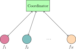
Figure 1: The federated architecture.

Consider the federated learning set-up stylized in Figure 1, in which $N$ agents and a coordinator cooperate towards the solution of the composite optimization problem

$$\bar{x}=\operatorname*{arg\,min}_{x\in\mathbb{R}^{n}}\ \sum_{i=1}^{N}f_{i}(x)+h(x)$$ (5)

where

$$f_{i}(x):=\frac{1}{q}\sum_{j=1}^{q}\ell_{i}\left(x;\xi_{i}^{(j)}\right)$$

is the local cost function of agent $i$ characterized by a local dataset $\mathcal{D}_{i}=\{\xi_{i}^{(1)},\dots,\xi_{i}^{(q)}\}$, $\ell_{i}(x,\xi)$ is the loss of the machine learning model over the data instance $\xi$, and $h:\mathbb{R}^{n}\to\mathbb{R}\cup\{+\infty\}$ is a common regularization function, which may be non-smooth. We introduce the following assumption.

Assumption 1.

The local loss functions $\ell_{i}$, $i\in\{1,\ldots,N\}$, are ${\underline{\lambda}}$-strongly convex and ${\bar{\lambda}}$-smooth with respect to the first argument. The cost $h$ is convex, closed, and proper, and it is proximable.

We remark that Assumption 1 implies that each $f_{i}$ is both ${\underline{\lambda}}$-strongly convex and ${\bar{\lambda}}$-smooth. In order to solve the problem in a federated set-up, the first step is to reformulate it into the following

$$\begin{split}\bar{\mathbold{x}}=&\operatorname*{arg\,min}_{\mathbold{x}\in\mathbb{R}^{nN}}\ \sum_{i=1}^{N}f_{i}(x_{i})+h(x_{1})\\ &\text{s.t.}\ x_{1}=\ldots=x_{N}\end{split}$$ (6)

where $x_{i}\in\mathbb{R}^{n}$ are local copies of $x$, and $\mathbold{x}=[x_{1}^{\top},\ldots,x_{N}^{\top}]$. The consensus constraint $x_{1}=\ldots=x_{N}$ guarantees the equivalence of eq. 6 with eq. 5, and implies that $\bar{\mathbold{x}}=\boldsymbol{1}_{N}\otimes\bar{x}$, where $\bar{x}$ is the unique optimal solution of eq. 5. We can now rewrite eq. 6 in the following form

$$\bar{\mathbold{x}}=\operatorname*{arg\,min}_{\mathbold{x}\in\mathbb{R}^{nN}}f(\mathbold{x})+g(\mathbold{x})$$ (7)

with $f(\mathbold{x})=\sum_{i=1}^{N}f_{i}(x_{i})$, and $g(\mathbold{x})=\iota_{\mathbb{C}}(\mathbold{x})+h(x_{1}),$ where we imposed the consensus constraints through the indicator function of the consensus subspace

$$\mathbb{C}=\{\mathbold{x}=[x_{1}^{\top},\ldots,x_{N}^{\top}]\in\mathbb{R}^{nN}\ |\ x_{1}=\ldots=x_{N}\}.$$

In principle, eq. 7 could be now solved applying the Peaceman-Rachford splitting of eq. 3, but due to practical constraints (discussed in section III-B) this may not be possible. Instead, in section IV we will show how to use PRS as a template to design a federated algorithm that can be applied in practice.

III-B Design objectives

In this section we discuss some of the challenges that arise in federated learning set-ups, due to the practical constraints that they pose [1, 3]. The objective in the remainder of the paper then is to design and analyze an algorithm that can provably overcome these challenges.

Communication burden

In machine learning we are often faced with the task of training high-dimensional models, with deep neural networks the foremost example. This implies that problem eq. 5 may be characterized by $n\gg 1$. In a federated set-up then, sharing models between the agents and the coordinator imposes a significant communication burden [15]. Initial approaches to federated learning therefore introduced different techniques to reduce the number of communications required, such as local training [3]. Local training requires that, before a round of communications, each agent perform multiple steps (or epochs) of minimization of the local loss function. Employing local training, however, may result in worse accuracy, especially when the loss functions of the agents are heterogeneous. The objective then is to design federated algorithms that perform local training without jeopardizing accuracy of the trained model, see e.g. [29, 30, 31, 14, 32].

Heterogeneous agents

The devices involved in the federated learning process may be in general very heterogeneous as regards to computational, storage, and communication capabilities. Indeed, these devices may be equipped with very different hardware (CPU, memory, battery), and they may be using different network connectivity (mobile or Wi-Fi) [1, 3]. The heterogeneity of the agents’ resources implies that they may perform local computations, and transmit their results, at different rates. This results in partial participation, with only a subset of the agents being active at any given time. Besides arising from practical limitations, partial participation may also be enforced in order to relieve the communication burden. The goal therefore is to design a federated algorithm that allows for partial participation while preserving accuracy of the trained model.

Privacy

The leakage of private information through machine learning models’ parameters and predictions has been extensively documented [9, 10, 11]. One notable example is the support vector machine (SVM) in its dual form, where the solution involves a linear combination of specific data points. Recently, there has been a growing interest in iterative randomized training algorithms that offer privacy-preserving guarantees [20, 21], such as RDP and ADP. However, the existing results suffer from privacy loss that increases over training epochs [40] and fail to support local training and the partial participation of heterogeneous agents [20]. These limitations make it challenging to extend those approaches to the specific setup addressed in this work. The objective of this study is to address these challenges by providing a rigorous privacy-preserving guarantee that remains bounded over time and is compatible with the federated learning setup under consideration.

To summarize, the goal of this paper is to design a federated algorithm with the following features:

1. Local training: the algorithm should allow for multiple epochs of local training, but without jeopardizing accuracy of the computed solution.

2. Partial participation: the algorithm should allow for a subset of the agents to be active at any time, again without jeopardizing accuracy.

3. Privacy: the algorithm should incorporate a privacy mechanism to safeguard the local training data.

IV Algorithm Design

In this section we derive and discuss the proposed Algorithm 1, highlighting the different design choices that it allows for.

Algorithm 1 Federated Private Local Training (Fed-PLT)

1:For each agent initialize $x_{i,0}$ and $z_{i,0}$; choose the local solver, its parameters, and the number of local epochs ${N_{\mathrm{e}}}$; the parameter $\rho>0$

2:$x_{i,K}$

3:for $k=0,1,\ldots,K$ each agent $i$ do

4:     // coordinator

5:     the coordinator averages the information received from the agents

$$y_{k+1}=\operatorname{prox}_{\rho h/N}\left(\frac{1}{N}\sum_{i=1}^{N}z_{i,k}\right)$$

and transmits it to all agents

6:     // agents

7:     for $i=1,\ldots,N$ do

8:         if agent $i$ is active then

9:              set $w_{i,k}^{0}=x_{i,k}$, $v_{i,k}=2y_{k+1}-z_{i,k}$

10:              for $\ell=0,1,\ldots,{N_{\mathrm{e}}}-1$ do $\triangleright$ local solver

11:                  e.g. gradient descent

$$w_{i,k}^{\ell+1}=w_{i,k}^{\ell}-\gamma\left(\nabla f_{i}(w_{i,k}^{\ell})+\frac{1}{\rho}(w_{i,k}^{\ell}-v_{i,k})\right)$$

12:              end for

13:              set $x_{i,k+1}=w_{i,k}^{{N_{\mathrm{e}}}}$

14:              update the auxiliary variable

$$z_{i,k+1}=z_{i,k}+2(x_{i,k+1}-y_{k+1})$$

and transmit to coordinator

15:         else$\triangleright$ inactive agent

16:              set $x_{i,k+1}=x_{i,k}$ and $z_{i,k+1}=z_{i,k}$

17:         end if

18:     end for

19:     

20:end for

IV-A Algorithm derivation

We start by applying the PRS of eq. 3 to the federated optimization problem eq. 7, which yields

$$\mathbold{y}_{k+1} =\operatorname{prox}_{\rho g}(\mathbold{z}_{k})$$ (8a)

$$\mathbold{x}_{k+1} =\operatorname{prox}_{\rho f}(2\mathbold{y}_{k+1}-\mathbold{z}_{k})$$ (8b)

$$\mathbold{z}_{k+1} =\mathbold{z}_{k}+2(\mathbold{x}_{k+1}-\mathbold{y}_{k+1}),$$ (8c)

We now discuss the implementation of eq. 8a and eq. 8b in turn.

IV-A1 Implementation of eq. 8a

First of all, update eq. 8a can be computed by the coordinator using the information it receives from all the agents and the fact that $h$ is proximable, as detailed in Lemma 6.

Lemma 6 ($\operatorname{prox}_{\rho g}$ computation).

The proximal of $g(\mathbold{x})=\iota_{\mathbb{C}}(\mathbold{x})+h(x_{1})$ at a point $\mathbold{z}\in\mathbb{R}^{nN}$ is given by

$$\operatorname{prox}_{\rho g}(\mathbold{z})=\boldsymbol{1}_{N}\otimes\operatorname{prox}_{\rho h/N}\left(\frac{1}{N}\sum_{i=1}^{N}z_{i}\right).$$

Proof.

By Definition 3, to compute the proximal of $g$ we need to solve:

$$\operatorname{prox}_{\rho g}(\mathbold{z})=\operatorname*{arg\,min}_{\mathbold{x}\in\mathbb{R}^{nN}}\left\{\iota_{\mathbb{C}}(\mathbold{x})+h(x_{1})+\frac{1}{2\rho}\left\lVert\mathbold{x}-\mathbold{z}\right\rVert^{2}\right\}$$

$$\overset{(i)}{=}\boldsymbol{1}\otimes\operatorname*{arg\,min}_{x\in\mathbb{R}^{n}}\left\{h(x)+\frac{1}{2\rho}\sum\nolimits_{i}\left\lVert x-z_{i}\right\rVert^{2}\right\}$$

$$\overset{(ii)}{=}\boldsymbol{1}\otimes\operatorname*{arg\,min}_{x\in\mathbb{R}^{n}}\left\{h(x)+N\frac{1}{2\rho}\left\lVert x-\frac{1}{N}\sum\nolimits_{i}z_{i}\right\rVert^{2}\right\}$$

$$=\boldsymbol{1}\otimes\operatorname{prox}_{\rho h/N}\left(\frac{1}{N}\sum\nolimits_{i}z_{i}\right)$$

where (i) follows by using $\mathbold{x}=\boldsymbol{1}\otimes x$ to enforce the consensus constraints, (ii) follows by manipulations of the quadratic regularization and adding and summing terms that do not depend on $x$. ∎

Given the result of Lemma 6, the coordinator is therefore tasked with storing and updating the variable

$$y_{k+1}=\operatorname{prox}_{\rho h/N}\left(\frac{1}{N}\sum_{i=1}^{N}z_{i,k}\right)$$

for which $\mathbold{y}_{k+1}=\boldsymbol{1}_{N}\otimes y_{k+1}$.

IV-A2 Implementation of eq. 8b

Computing eq. 8b instead is a task for the agents, as the update depends on the private local costs. In particular, letting $\mathbold{v}_{k}=2\mathbold{y}_{k+1}-\mathbold{z}_{k}$, we notice that the update eq. 8b requires the solution of

$$\min_{\mathbold}{x}\sum_{i=1}^{N}f_{i}(x_{i})+\frac{1}{2\rho}\left\lVert\mathbold{x}-\mathbold{v}_{k}\right\rVert^{2}=$$ (9)

$$\hskip 28.45274pt=\sum_{i=1}^{N}\min_{x_{i}}f_{i}(x_{i})+\frac{1}{2\rho}\left\lVert x_{i}-v_{i,k}\right\rVert^{2}=:d_{i,k}(x_{i}),$$

where $v_{i,k}=2y_{k+1}-z_{i,k}$. Since the problem can be decoupled, each agent needs to locally solve the corresponding minimization $\min_{x_{i}}d_{i,k}(x_{i})$, which yields the local state update

$$x_{i,k+1}=\operatorname{prox}_{\rho f_{i}}(v_{i,k})=\operatorname*{arg\,min}_{x_{i}\in\mathbb{R}^{n}}d_{i,k}(x_{i}).$$ (10)

However, in general eq. 10 does not have a closed form solution, and the agents can only approximate the update via a finite number of local training epochs. As a first approach, each agent can apply ${N_{\mathrm{e}}}\in\mathbb{N}$ steps of gradient descent (cf. Lemma 2) to approximate the local update:

$$\begin{split}w_{i,k}^{0}&=x_{i,k}\\ w_{i,k}^{\ell+1}&=w_{i,k}^{\ell}-\gamma\nabla d_{i,k}(w_{i,k}^{\ell})\quad\ell=0,\ldots,{N_{\mathrm{e}}}-1\\ x_{i,k+1}&=w_{i,k}^{N_{\mathrm{e}}}\end{split}$$ (11)

where $\gamma\in(0,2/({\underline{\lambda}}+1/\rho))$, since $d_{i,k}\in\mathcal{F}_{{\underline{\lambda}}+1/\rho,{\bar{\lambda}}+1/\rho}\left(\mathbb{R}^{n}\right)$. More generally, one can apply any suitable local solver to compute eq. 10, as discussed in section IV-B. In particular, the choice of local solver can be leveraged to enhance privacy.

Finally, in the derivation above, each agent approximates its local proximal at each iteration $k\in\mathbb{N}$. However, this is not required, as Algorithm 1 allows for only a subset of active agents to share the results of their local training at iteration $k\in\mathbb{N}$; this feature is discussed in section IV-C.

To summarize, the proposed Algorithm 1 provides two flexible design choices in the following key aspects:

1. local training: during local training, any suitable solver can be employed by the agents, including privacy preserving methods (objectives (i) and (iii));

2. partial participation: the algorithm allows for a subset of the agents to be active at any given time $k\in\mathbb{N}$ (objective (ii)).

IV-B Local training methods

In principle, one may choose to use any suitable local solver to approximate the solution of $\min_{x_{i}}d_{i,k}(x_{i})=f_{i}(x_{i})+(1/2\rho)\left\lVert x_{i}-v_{i,k}\right\rVert^{2}$. This problem is especially amenable since it is strongly convex, with $d_{i,k}\in\mathcal{F}_{{\underline{\lambda}}+1/\rho,{\bar{\lambda}}+1/\rho}\left(\mathbb{R}^{n}\right)$. A first option is the gradient descent, already discussed in eq. 11. Notice that by Lemma 2 we know that the gradient descent is contractive with rate $\chi=\max\{|1-\gamma({\underline{\lambda}}+1/\rho)|,|1-\gamma({\bar{\lambda}}+1/\rho)|\}$, which is minimized by choosing $\gamma=2/({\bar{\lambda}}+{\underline{\lambda}}+2/\rho)$. In the following, we discuss some alternatives that address different design objectives.

Accelerated gradient descent

Improving the performance of local training can be achieved by using the accelerated gradient descent, see e.g. [41, Algorithm 14], characterized by

$$\begin{split}w_{i,k}^{0}&=x_{i,k},\ u_{i}^{0}=w_{i,k}^{0}\\ u_{i}^{\ell+1}&=w_{i,k}^{\ell}-\frac{1}{{\bar{\lambda}}}\nabla d_{i,k}(w_{i,k}^{\ell})\quad\ell=0,\ldots,{N_{\mathrm{e}}}-1\\ w_{i,k}^{\ell+1}&=u_{i}^{\ell+1}+\frac{\sqrt{{\bar{\lambda}}}-\sqrt{{\underline{\lambda}}}}{\sqrt{{\bar{\lambda}}}+\sqrt{{\underline{\lambda}}}}(u_{i}^{\ell+1}-u_{i}^{\ell})\\ x_{i,k+1}&=w_{i,k}^{N_{\mathrm{e}}},\end{split}$$ (12)

which employs constant step-sizes owing to the strong convexity of $d_{i,k}$. Local solvers with even better performance can also be chosen, for example (quasi-)Newton methods.

Stochastic gradient descent

Both gradient descent and accelerated gradient descent rely on the use of full gradient evaluations, which may be too computationally expensive in learning applications. Therefore, the agents may resort to stochastic gradient descent (SGD) methods [36], which employ approximated gradients during the local training. Recalling that the local costs are defined as $f_{i}(x):=\frac{1}{q}\sum_{j=1}^{q}\ell_{i}(x;\xi_{i}^{(j)}),$ SGD makes use of the following approximate gradient

$$\hat{\nabla}f_{i}(x)=\frac{1}{q}\sum_{j\in\mathcal{B}}\nabla\ell_{i}(x;\xi_{i}^{(j)})$$

where $\mathcal{B}\subset\{1,\ldots,q\}$ are the indices of a subset of data points chosen at random.

Private local training

The previous local solvers address performance concerns; however, when the design objective is privacy preservation, the agents should resort to the use of noisy gradient descent [20, 42]. In particular, the update of $w_{i,k}^{\ell+1}$ in eq. 11 is perturbed with Gaussian noise:

$$\begin{split}w_{i,k}^{\ell+1}&=w_{i,k}^{\ell}-\gamma\nabla d_{i,k}(w_{i,k}^{\ell})+t_{i,k}^{\ell}\\ t_{i,k}^{\ell}&\sim\sqrt{2\gamma}\mathcal{N}(0,\tau^{2}{I}_{n})\end{split}$$ (13)

where $\ell=0,\ldots,{N_{\mathrm{e}}}-1$, and $\tau^{2}>0$ is the noise variance. The addition of a stochastic additive noise in each iteration of eq. 13 allows us to establish rigorous differential privacy guarantees, which can be tuned by selecting the variance $\tau^{2}$.

Remark 1 (Uncoordinated local solvers).

In this section we only discussed the case of “coordinated” local solvers, that is, all agents use the same solver with the same parameters (e.g. gradient with common – or coordinated – step-size $\gamma$). The results of section V actually allow for uncoordinated solvers, with the agents either using different algorithms, or the same algorithm with different parameters. For example, if the local costs are such that $f_{i}\in\mathcal{F}_{{\underline{\lambda}}_{i},{\bar{\lambda}}_{i}}\left(\mathbb{R}^{n}\right)$, then the local step-size can be tuned using the strong convexity and smoothness moduli of $f_{i}$, instead of the global moduli ${\underline{\lambda}}=\min_{i}{\underline{\lambda}}_{i}$, ${\bar{\lambda}}=\max_{i}{\bar{\lambda}}_{i}$. This is especially useful because it means that the algorithm can adapt to the heterogeneity of the local costs.

IV-C Partial participation

As discussed in section III-B, there are different reasons why only a subset of the agents may participate at any given time $k\in\mathbb{N}$. On the one hand, the heterogeneity of the agents’ hardware (CPU, battery, connectivity, …) may result in different paces of local training. This means that not all agents will conclude their computations at the same time, and the coordinator will receive new results only from those that did. On the other hand, partial participation can be introduced by design in order to reduce the communication burden. In this case, the coordinator picks a (random) subset of the agents and requests that they send the new results of local training, thus reducing the number of communications exchanged. This scheme is often referred to as client selection [14].

The proposed Algorithm 1 allows for any partial participation, be it intrinsic (due to heterogeneity of the agents) or extrinsic (due to client selection). In particular, the only requirement, detailed in Assumption 2, is that at any given time an agent $i$ participates in the learning with a given fixed probability $p_{i}\in(0,1]$.

V Convergence Analysis

In this section we prove the convergence of Algorithm 1. We start by showing that the proposed algorithm can be interpreted as a contractive operator. Then, building on this result we characterize convergence for the different local training choices discussed in section IV-B.

V-A Contractiveness of Algorithm 1

The goal of this section is to show that Algorithm 1 can be characterized as a contractive operator, similarly to the PRS from which it was derived. First of all, we remark that $y_{k+1}$ only depends on $\mathbold{z}_{k}$, and hence we can represent Algorithm 1 in terms of $\mathbold{x}$ and $\mathbold{z}$ only. In particular, letting $\mathcal{X}:\mathbb{R}^{nN}\times\mathbb{R}^{nN}\to\mathbb{R}^{nN}:(\mathbold{x}_{k},\mathbold{z}_{k})\mapsto\mathbold{x}_{k+1}$ be the map denoting the local updates, and assuming that all agents are active, we can write

$$\begin{bmatrix}\mathbold{x}_{k+1}\\ \mathbold{z}_{k+1}\end{bmatrix}=\begin{bmatrix}\mathcal{X}(\mathbold{x}_{k},\mathbold{z}_{k})\\ \mathbold{z}_{k}+2(\mathbold{x}_{k+1}-\operatorname{prox}_{\rho g}(\mathbold{z}_{k}))\end{bmatrix}=\mathcal{T}\begin{bmatrix}\mathbold{x}_{k}\\ \mathbold{z}_{k}\end{bmatrix}$$

The following Proposition 1 proves that $\mathcal{T}$ is contractive for a suitable choice of local solver.

Proposition 1 (Algorithm 1 is contractive).

Let the local solvers be $\chi^{N_{\mathrm{e}}}$-contractive in the first argument, that is

$$\left\lVert\mathcal{X}(\mathbold{x},\mathbold{z}_{k})-\mathcal{X}(\mathbold{y},\mathbold{z}_{k})\right\rVert\leq\chi^{N_{\mathrm{e}}}\left\lVert\mathbold{x}-\mathbold{y}\right\rVert,\quad\forall\mathbold{x},\mathbold{y}\in\mathbb{R}^{n},$$

and let the PRS applied to eq. 6 be $\zeta$-contractive (cf. Lemma 3) with fixed point $\bar{\mathbold{z}}$. Let the parameters $\rho$ and ${N_{\mathrm{e}}}$ be chosen such that the following matrix is stable:

$$S=\begin{bmatrix}\chi^{N_{\mathrm{e}}}&\frac{1+\chi^{N_{\mathrm{e}}}}{{\underline{\lambda}}+1/\rho}\\ 2\chi^{N_{\mathrm{e}}}&\zeta+\frac{2\chi^{N_{\mathrm{e}}}}{{\underline{\lambda}}+1/\rho}\end{bmatrix}.$$

Then the operator $\mathcal{T}:\mathbb{R}^{nN}\times\mathbb{R}^{nN}\to\mathbb{R}^{nN}\times\mathbb{R}^{nN}$ characterizing Algorithm 1 is contractive. The contraction constant of $\mathcal{T}$ is upper bounded by $\left\lVert S\right\rVert$, and its unique fixed point is $[\bar{\mathbold{x}}^{\top},\bar{\mathbold{z}}^{\top}]^{\top}$, where $\bar{\mathbold{x}}$ is the optimal solution to eq. 6.

Proof.

1) Fixed point: We start by showing that $[\bar{\mathbold{x}}^{\top},\bar{\mathbold{z}}^{\top}]^{\top}$ is indeed a fixed point for $\mathcal{T}$. By Lemma 3, the PRS applied to eq. 6 is contractive, since $f\in\mathcal{F}_{{\underline{\lambda}},{\bar{\lambda}}}\left(\mathbb{R}^{nN}\right)$, and its fixed point $\bar{\mathbold{z}}$ is such that

$$\bar{\mathbold{x}}=\operatorname{prox}_{\rho g}(\bar{\mathbold{z}})=\operatorname{prox}_{\rho f}(2\bar{\mathbold{x}}-\bar{\mathbold{z}}).$$

Therefore, defining $d(\mathbold{x};\mathbold{z})=f(\mathbold{x})+\frac{1}{2\rho}\left\lVert\mathbold{x}-\mathbold{z}\right\rVert^{2}$ we have

$$\bar{\mathbold{x}} =\operatorname*{arg\,min}_{\mathbold}{x}d(\mathbold{x};\operatorname{refl}_{\rho g}(\bar{\mathbold{z}}))$$

$$=\operatorname*{arg\,min}_{\mathbold}{x}d(\mathbold{x};2\operatorname{prox}_{\rho g}(\bar{\mathbold{z}})-\bar{\mathbold{z}}).$$

But this implies that, if we initialize the local updates of Algorithm 1 at $\bar{\mathbold{x}},\bar{\mathbold{z}}$, then they will return $\bar{\mathbold{x}}$ itself, since it is the stationary point of $d(\cdot;\operatorname{refl}_{\rho g}(\bar{\mathbold{z}}))$. This fact, in addition to the fact that $\bar{\mathbold{z}}$ is the fixed point of the PRS eq. 8, proves that indeed $[\bar{\mathbold{x}}^{\top},\bar{\mathbold{z}}^{\top}]^{\top}=\mathcal{T}[\bar{\mathbold{x}}^{\top},\bar{\mathbold{z}}^{\top}]^{\top}.$

2) Contractiveness: We proceed now by proving that $\mathcal{T}$ is contractive, and characterizing its contraction rate. We do this by deriving bounds to the distances $\left\lVert\mathbold{x}_{k+1}-\bar{\mathbold{x}}\right\rVert$ and $\left\lVert\mathbold{z}_{k+1}-\bar{\mathbold{z}}\right\rVert$.

We start by providing the following auxiliary result. By the discussion above we know that $\bar{\mathbold{x}}=\operatorname*{arg\,min}_{\mathbold}{x}d(\mathbold{x};\operatorname{refl}_{\rho g}(\bar{\mathbold{z}}))$, and similarly the exact local update eq. 8b is given by $\bar{\mathbold{x}}_{k+1}=\operatorname*{arg\,min}_{\mathbold}{x}d(\mathbold{x};\operatorname{refl}_{\rho g}(\mathbold{z}_{k}))$. But since $d$ is $({\underline{\lambda}}+1/\rho)$-strongly convex in $\mathbold{x}$, we can apply the implicit function theorem [44, Theorem 1B.1] to prove that

$$\left\lVert\bar{\mathbold{x}}_{k+1}-\bar{\mathbold{x}}\right\rVert \leq\frac{1}{{\underline{\lambda}}+1/\rho}\left\lVert\operatorname{refl}_{\rho g}(\mathbold{z}_{k})-\operatorname{refl}_{\rho g}(\bar{\mathbold{z}})\right\rVert$$

$$\overset{(i)}{\leq}\frac{1}{{\underline{\lambda}}+1/\rho}\left\lVert\mathbold{z}_{k}-\bar{\mathbold{z}}\right\rVert$$ (14)

where (i) holds by the fact that the reflective operator is non-expansive [45].

With this result in place, we can now derive the following chain of inequalities:

$$\left\lVert\mathbold{x}_{k+1}-\bar{\mathbold{x}}\right\rVert \overset{(i)}{\leq}\left\lVert\mathbold{x}_{k+1}-\bar{\mathbold{x}}_{k+1}\right\rVert+\left\lVert\bar{\mathbold{x}}_{k+1}-\bar{\mathbold{x}}\right\rVert$$

$$\overset{(ii)}{\leq}\left\lVert\mathbold{x}_{k+1}-\bar{\mathbold{x}}_{k+1}\right\rVert+\frac{1}{{\underline{\lambda}}+1/\rho}\left\lVert\mathbold{z}_{k}-\bar{\mathbold{z}}\right\rVert$$

$$\overset{(iii)}{\leq}\chi^{N_{\mathrm{e}}}\left\lVert\mathbold{x}_{k}-\bar{\mathbold{x}}_{k+1}\right\rVert+\frac{1}{{\underline{\lambda}}+1/\rho}\left\lVert\mathbold{z}_{k}-\bar{\mathbold{z}}\right\rVert$$ (15)

where (i) holds by triangle inequality, (ii) by eq. 14, and (iii) by contractiveness of the local solvers. By again using the triangle inequality and eq. 14 we have

$$\left\lVert\mathbold{x}_{k}-\bar{\mathbold{x}}_{k+1}\right\rVert \leq\left\lVert\mathbold{x}_{k}-\bar{\mathbold{x}}\right\rVert+\left\lVert\bar{\mathbold{x}}-\bar{\mathbold{x}}_{k+1}\right\rVert$$

$$\leq\left\lVert\mathbold{x}_{k}-\bar{\mathbold{x}}\right\rVert+\frac{1}{{\underline{\lambda}}+1/\rho}\left\lVert\mathbold{z}_{k}-\bar{\mathbold{z}}\right\rVert,$$

and substituting into eq. 15 we get

$$\left\lVert\mathbold{x}_{k+1}-\bar{\mathbold{x}}\right\rVert\leq\chi^{N_{\mathrm{e}}}\left\lVert\mathbold{x}_{k}-\bar{\mathbold{x}}\right\rVert+\frac{1+\chi^{N_{\mathrm{e}}}}{{\underline{\lambda}}+1/\rho}\left\lVert\mathbold{z}_{k}-\bar{\mathbold{z}}\right\rVert.$$ (16)

We turn now to bounding $\left\lVert\mathbold{z}_{k+1}-\bar{\mathbold{z}}\right\rVert$. By the updates characterizing Algorithm 1 we can write

$$\mathbold{z}_{k+1}=\mathbold{z}_{k}+2\left(\mathbold{x}_{k+1}-\operatorname{prox}_{\rho g}(\mathbold{z}_{k})\right)$$

$$=\mathbold{z}_{k}+2\left(\bar{\mathbold{x}}_{k+1}-\operatorname{prox}_{\rho g}(\mathbold{z}_{k})\right)+2(\mathbold{x}_{k+1}-\bar{\mathbold{x}}_{k+1})$$

$$=\mathcal{T}_{\mathrm{PR}}\mathbold{z}_{k}+2(\mathbold{x}_{k+1}-\bar{\mathbold{x}}_{k+1})$$

where recall that $\bar{\mathbold{x}}_{k+1}$ denotes the exact local updates, and $\mathcal{T}_{\mathrm{PR}}$ denotes the exact PRS.

We can then derive the following bound:

$$\left\lVert\mathbold{z}_{k+1}-\bar{\mathbold{z}}\right\rVert\overset{(i)}{\leq}\left\lVert\mathcal{T}_{\mathrm{PR}}\mathbold{z}_{k}-\bar{\mathbold{z}}\right\rVert+2\left\lVert\mathbold{x}_{k+1}-\bar{\mathbold{x}}_{k+1}\right\rVert$$

$$\qquad\overset{(ii)}{\leq}\zeta\left\lVert\mathbold{z}_{k}-\bar{\mathbold{z}}\right\rVert+2\left\lVert\mathbold{x}_{k+1}-\bar{\mathbold{x}}_{k+1}\right\rVert$$

$$\qquad\overset{(iii)}{\leq}\left(\zeta+\frac{2\chi^{N_{\mathrm{e}}}}{{\underline{\lambda}}+1/\rho}\right)\left\lVert\mathbold{z}_{k}-\bar{\mathbold{z}}\right\rVert+2\chi^{N_{\mathrm{e}}}\left\lVert\mathbold{x}_{k}-\bar{\mathbold{x}}\right\rVert$$ (17)

where (i) holds by triangle inequality, (ii) by the PRS operator $\mathcal{T}_{\mathrm{PR}}$ being contractive by Lemma 3, and (iii) by an argument similar to that leading to eq. 16 and rearranging.

Finally, putting eqs. 16 and 17 together yields

$$\begin{bmatrix}\left\lVert\mathbold{x}_{k+1}-\bar{\mathbold{x}}\right\rVert\\ \left\lVert\mathbold{z}_{k+1}-\bar{\mathbold{z}}\right\rVert\end{bmatrix}\leq S\begin{bmatrix}\left\lVert\mathbold{x}_{k}-\bar{\mathbold{x}}\right\rVert\\ \left\lVert\mathbold{z}_{k}-\bar{\mathbold{z}}\right\rVert\end{bmatrix}$$

and taking the square norm on both sides

$$\left\lVert\mathbold{x}_{k+1}-\bar{\mathbold{x}}\right\rVert^{2}+\left\lVert\mathbold{z}_{k+1}-\bar{\mathbold{z}}\right\rVert^{2}\leq\left\lVert S\begin{bmatrix}\left\lVert\mathbold{x}_{k}-\bar{\mathbold{x}}\right\rVert\\ \left\lVert\mathbold{z}_{k}-\bar{\mathbold{z}}\right\rVert\end{bmatrix}\right\rVert^{2}$$

$$\qquad\leq\left\lVert S\right\rVert^{2}\left(\left\lVert\mathbold{x}_{k}-\bar{\mathbold{x}}\right\rVert^{2}+\left\lVert\mathbold{z}_{k}-\bar{\mathbold{z}}\right\rVert^{2}\right).$$

Therefore by Definition 2 this proves that Algorithm 1 is indeed contractive. ∎

Remark 2 (The importance of initialization).

Initializing the local update computation eq. 11 with $w_{i,k}^{0}=x_{i,k}$ is fundamental to guarantee contractiveness of Algorithm 1, and thus its convergence, as detailed in the following section V-B.

V-B Convergence results

Proposition 1 proved that Algorithm 1 can be modeled as a contractive operator when all the agents are active. This fact then would allow us to characterize the convergence of the algorithm by using Banach-Picard theorem (cf. Lemma 1). However, in this section we are interested in analyzing convergence with partial participation, that is, when only a (random) subset of agents is active at each time $k\in\mathbb{N}$. In addition to partial participation, we are interested in convergence when a further source of stochasticity is present: inexact local solvers. In section IV-B we have indeed discussed two local solvers that, either due to computational constraints or privacy concerns, introduce inexactness during training.

To account for both partial participation and inexact local training, we can write Algorithm 1 as the following stochastic update

$$\begin{bmatrix}x_{i,k+1}\\ z_{i,k+1}\end{bmatrix}=\begin{cases}\begin{bmatrix}\mathcal{X}_{i}(x_{i,k},\mathbold{z}_{k})\\ z_{i,k}+2(\mathcal{X}_{i}(x_{i,k},\mathbold{z}_{k})-y_{k+1})\end{bmatrix}+e_{i,k}\\ \hskip 142.26378pt\text{if}\ u_{i,k}=1\\ \begin{bmatrix}x_{i,k}\\ z_{i,k}\end{bmatrix}\hskip 113.81102pt\text{if}\ u_{i,k}=0\end{cases}$$ (18)

where $u_{i,k}\sim Ber(p_{i})$ is the r.v. which equals $1$ when agent $i$ is active at time $k$, $\mathcal{X}_{i}$ denotes the $i$-th component of the local updates map $\mathcal{X}$, and $e_{i,k}$ is a random additive noise modeling inexact local updates.

We can now formalize the stochastic set-up of eq. 18 as follows, which will then allow convergence analysis with the tools of section II-C.

Assumption 2 (Stochastic set-up).

2. The random variables $\{u_{i,k}\}_{k\in\mathbb{N}}$ are i.i.d. Bernoulli with mean $p_{i}\in(0,1]$, for any $i=1,\ldots,N$.

3. Let $\mathbold{e}_{k}=[e_{1,k}^{\top},\ldots,e_{N,k}^{\top}]^{\top}$ be the random vector collecting all additive errors. We assume that $\{\mathbold{e}_{k}\}_{k\in\mathbb{N}}$ are i.i.d. and such that $\mathbb{E}\left[\left\lVert\mathbold{e}_{k}\right\rVert\right]=\nu<\infty$.

4. For every $k\in\mathbb{N}$, $\{u_{i,k}\}_{i=1}^{N}$ and $\mathbold{e}_{k}$ are independent.

We are now ready to prove convergence of Algorithm 1.

Proposition 2 (Convergence).

Let the parameters of Algorithm 1 be such that Proposition 1 holds, and let Assumption 2 be verified. Then the sequence $\{[\mathbold{x}_{k}^{\top},\mathbold{z}_{k}^{\top}]^{\top}\}_{k\in\mathbb{N}}$ generated by the algorithm satisfies the following bound

$$\mathbb{E}\left[\left\lVert\begin{bmatrix}\mathbold{x}_{k}-\bar{\mathbold{x}}\\ \mathbold{z}_{k}-\bar{\mathbold{z}}\end{bmatrix}\right\rVert\right]\leq\sqrt{\frac{\bar{p}}{\underaccent{\bar}{p}}}\left(\sigma^{k}\left\lVert\begin{bmatrix}\mathbold{x}_{0}-\bar{\mathbold{x}}\\ \mathbold{z}_{0}-\bar{\mathbold{z}}\end{bmatrix}\right\rVert+\frac{1-\sigma^{k}}{1-\sigma}\nu\right)$$

where $\underaccent{\bar}{p}=\min_{i}p_{i}$, $\bar{p}=\max_{i}p_{i}$, and $\sigma=\sqrt{1-\underaccent{\bar}{p}+\underaccent{\bar}{p}\left\lVert S\right\rVert^{2}}$.

Proof.

If Proposition 1 is verified, then the algorithm is contractive, and under Assumption 2 we can apply the stochastic Banach-Picard of Lemma 4. ∎

Proposition 2 proves that, for a suitable choice of parameters, Algorithm 1 converges when the agents apply (stochastic) gradient descent during local training. The following result shows that convergence is achieved also when the agents employ the accelerated gradient descent as a local solver.

Proposition 3 (Convergence with accelerated gradient).

Let the agents employ the accelerated gradient as local solver. Let the parameters $\rho$ and ${N_{\mathrm{e}}}$ be chosen such that the following matrix is stable:

$$S^{\prime}=\begin{bmatrix}\chi({N_{\mathrm{e}}})&\frac{1+\chi({N_{\mathrm{e}}})}{{\underline{\lambda}}+1/\rho}\\ 2\chi({N_{\mathrm{e}}})&\zeta+\frac{2\chi({N_{\mathrm{e}}})}{{\underline{\lambda}}+1/\rho}\end{bmatrix}$$

where

$$\chi({N_{\mathrm{e}}}):=\left(1+{\bar{\lambda}}/{\underline{\lambda}}\right)\left(1-\sqrt{{\underline{\lambda}}/{\bar{\lambda}}}\right)^{N_{\mathrm{e}}}.$$

Then the operator $\mathcal{T}^{\prime}:\mathbb{R}^{nN}\times\mathbb{R}^{nN}\to\mathbb{R}^{nN}\times\mathbb{R}^{nN}$ characterizing Algorithm 1 (with accelerated gradient) is contractive and, under Assumption 2, Proposition 2 holds.

Proof.

The contractiveness of Algorithm 1 with accelerated gradient as local solver follows along the lines of the proof of Proposition 1, with $\chi^{N_{\mathrm{e}}}$ being replaced by $\chi({N_{\mathrm{e}}})$. Indeed, by Lemma 7 in the Appendix the local update map $\mathcal{X}^{\prime}$ verifies

$$\left\lVert\mathcal{X}(\mathbold{x},\mathbold{z}_{k})-\mathcal{X}(\mathbold{y},\mathbold{z}_{k})\right\rVert\leq\chi({N_{\mathrm{e}}})\left\lVert\mathbold{x}-\mathbold{y}\right\rVert,\quad\forall\mathbold{x},\mathbold{y}\in\mathbb{R}^{n}.$$

The convergence under Assumption 2 is thus another consequence of Lemma 4. ∎

Remark 3 (Exact convergence).

Notice that when exact local solvers are employed (hence $\nu=0$ in Assumption 2) then Propositions 2 and 3 prove exact convergence to the fixed point $[\bar{\mathbold{x}}^{\top}\ \bar{\mathbold{z}}^{\top}]^{\top}$, even in the presence of partial participation. As a consequence, the proposed algorithm indeed allows for the use of local training without degrading accuracy (objective (i) in section III-B).

VI Privacy Analysis

In this section, we prove that Algorithm 1, utilizing the noisy gradient descent eq. 13 as local training method, guarantees RDP for every data sample in $\mathcal{D}:=\cup_{i=1}^{N}\mathcal{D}_{i}$. We will derive this result in the case of full agents’ participation, which can provide an upper bound to the privacy guarantee with partial participation. Before proceeding to the analysis, we make the following assumption.

Assumption 3 (Sensitivity).

For each $i\in\{1,\ldots,N\}$, there exists some $L>0$ such that

$$\left\lVert\nabla f_{i}^{\mathcal{D}_{i}}(x)-\nabla f_{i}^{\mathcal{D}^{\prime}_{i}}(x)\right\rVert\leq\frac{L}{q},\quad\forall x\in\mathbb{R}^{n}$$

where $\nabla f_{i}^{\mathcal{D}_{i}}$ denotes the gradient of $f_{i}$ induced by the dataset $\mathcal{D}_{i}$, and $\mathcal{D}_{i}$ and $\mathcal{D}^{\prime}_{i}$ are neighboring datasets of size $q$.

Assumption 3 quantifies the sensitivity of local gradient queries, which is a well-established concept in the field of machine learning with differential privacy [20, 42]. It is commonly satisfied in various learning problems, such as those involving $l_{2}$ regularized logistic loss (where the regularization ensures that Assumption 1 is also satisfied). For more general loss functions, the use of clipped gradients during training guarantees that Assumption 3 is verified [46]. Specifically, the gradients are clipped using the expression $\nabla\ell_{i}(x_{i};\xi_{i}^{(j)})\cdot\min\left\{1,\frac{L}{2\lVert\nabla\ell_{i}(x_{i};\xi_{i}^{(j)})\rVert}\right\}$, where $\xi_{i}^{(j)}\in\mathcal{D}_{i}$.

We are now ready to provide our privacy guarantee.

Proposition 4 (Privacy).

Suppose Assumptions 1 and 3 hold. Let the agents employ the noisy gradient descent eq. 13 with noise variance $\tau^{2}<\infty$ as local solver. If the step-size $\gamma<2/({\bar{\lambda}}+\rho^{-1})$ and each $x_{i,0}$ is drawn from $\mathcal{N}(0,2\tau^{2}I_{n}/{\underline{\lambda}})$, then Algorithm 1 satisfies $(\lambda,\varepsilon)$-Rényi differential privacy with

$$\varepsilon\leq\frac{\lambda L^{2}}{{\underline{\lambda}}\tau^{2}q^{2}}\left(1-e^{-{\underline{\lambda}}\gamma K{N_{\mathrm{e}}}/2}\right)$$

where $q$ is the number of local samples, ${\underline{\lambda}}$ and ${\bar{\lambda}}$ are the strong convexity modulus and smoothness parameter of the local cost, respectively.

Proof.

We denote by ${\mathbold{x}}_{k}:=[{x}^{\top}_{1,k},\ldots,{x}^{\top}_{N,k}]^{\top}$ and ${\mathbold{x}}_{k}^{\prime}:=[{x}^{\prime\top}_{1,k},\ldots,{x}^{\prime\top}_{N,k}]^{\top}$ the iterates produced by all the agents at the $k$’s iteration based on the neighboring datasets $\mathcal{D}$ and $\mathcal{D}^{\prime}$, respectively. Furthermore, let $\bm{X}_{k}$ and $\bm{X}^{\prime}_{k}$ be the corresponding random variables that model ${\mathbold{x}}_{k}$ and ${\mathbold{x}}_{k}^{\prime}$. We abuse the notation to also denote their probability distributions by $\bm{X}_{k}$ and $\bm{X}^{\prime}_{k}$. We are interested in the worst-case Rényi divergence between the output distributions based on $\mathcal{D}$ and $\mathcal{D}^{\prime}$, i.e., ${\rm D}_{\lambda}(\bm{X}_{K}||\bm{X}^{\prime}_{K})$. Since each agent generates the Gaussian noise independently, $x_{i,k}$ is independent between different $i$. In addition, two neighboring datasets $\mathcal{D}$ and $\mathcal{D}^{\prime}$ only have at most one data point that is different. Without loss of generality, we assume this different data point is possessed by agent $i$. Then, we obtain from [47, Theorem 27] that

$${\rm D}_{\lambda}(\bm{X}_{K}||\bm{X}^{\prime}_{K})={\rm D}_{\lambda}(\bm{X}_{i,K}||\bm{X}^{\prime}_{i,K}).$$

Next, we follow the approach in [20] to quantify the privacy loss during the local training process at the $k$’s iteration, that is, ${\rm D}_{\lambda}(\bm{X}_{i,k+1}||\bm{X}^{\prime}_{i,k+1})-{\rm D}_{\lambda}(\bm{X}_{i,k}||\bm{X}^{\prime}_{i,k})$. Recall that the local training update at the $\ell$-th step reads

$$\begin{split}&w_{i,k}^{\ell+1}=w_{i,k}^{\ell}-\gamma\nabla d_{i,k}(w_{i,k}^{\ell})+t_{i,k}^{\ell}\end{split}$$ (19)

where $w_{i,k}^{0}=x_{i,k}$ and $t_{i,k}^{\ell}\sim\sqrt{2\gamma}\mathcal{N}(0,\tau^{2}{I}_{n})$. Note that $d_{i,k}$ is $({\underline{\lambda}}+\rho^{-1})$-strongly convex and $({\bar{\lambda}}+\rho^{-1})$-smooth. Let $\bm{W}_{i,k}^{\gamma\ell}$ and $\bm{W}_{i,k}^{\prime\gamma\ell}$ be the probability distributions that model $w_{i,k}^{\ell}$ and $w_{i,k}^{\prime\ell}$. During the time interval $\gamma\ell<t<\gamma(\ell+1)$, the updates in eq. 19 on the datasets $\mathcal{D}$ and $\mathcal{D^{\prime}}$ are modeled using the following stochastic processes.

$$\left\{\begin{aligned} \bm{W}_{i,k}^{t}&=\bm{W}_{i,k}^{\gamma\ell}-\gamma U_{1}(\bm{W}_{i,k}^{\gamma\ell})-(t-\gamma\ell)U_{2}(\bm{W}_{i,k}^{\gamma\ell})\\ &\quad+\sqrt{2(t-\gamma\ell)\tau^{2}}\bm{G}^{\ell}\\ \bm{W}_{i,k}^{\prime t}&=\bm{W}_{i,k}^{\prime\gamma\ell}-\gamma U_{1}(\bm{W}_{i,k}^{\prime\gamma\ell})+(t-\gamma\ell)U_{2}(\bm{W}_{i,k}^{\prime\gamma\ell})\\ &\quad+\sqrt{2(t-\gamma\ell)\tau^{2}}\bm{G}^{\ell}\end{aligned}\right.$$ (20)

where $\bm{G}^{\ell}\sim\mathcal{N}(0,{I}_{n})$, $U_{1}(w_{i,k})=(\nabla d_{i,k}^{\mathcal{D}}(w_{i,k})+\nabla d_{i,k}^{\mathcal{D}^{\prime}}(w_{i,k}))/2$ and $U_{2}(w_{i,k})=(\nabla d_{i,k}^{\mathcal{D}}(w_{i,k})-\nabla d_{i,k}^{\mathcal{D}^{\prime}}(w_{i,k}))/2$. Conditioned on observing $w_{i,k}^{\ell}$, $w_{i,k}^{\prime\ell}$ and $v_{i,k}$, the diffusion processes in eq. 20 have the following stochastic differential equations

$$\begin{split}d\bm{W}_{i,k}^{t}&=-U_{2}(w_{i,k}^{\ell})dt+\sqrt{2\tau^{2}}d\bm{Z}^{t}\\ d\bm{W}_{i,k}^{\prime t}&=-U_{2}(w_{i,k}^{\prime\ell})dt+\sqrt{2\tau^{2}}d\bm{Z}^{t}\end{split}$$

where $d\bm{Z}^{t}\sim\sqrt{dt}\mathcal{N}(0,I_{n})$ describes the Wiener process.

For the training process at $k$’s iteration, we use Assumption 3 and a similar argument with (67) in [20, Theorem 2] to obtain

$$\begin{split}&\frac{{\rm D}_{\lambda}(\bm{W}^{{N_{\mathrm{e}}}}_{i,k}||\bm{W}^{\prime{N_{\mathrm{e}}}}_{i,k})}{\lambda}-\frac{L^{2}}{{\underline{\lambda}}\tau^{2}q^{2}}\\ &\leq\left(\frac{{\rm D}_{\lambda_{k}}(\bm{W}^{0}_{i,k}||\bm{W}^{\prime 0}_{i,k})}{\lambda_{k}}-\frac{L^{2}}{{\underline{\lambda}}\tau^{2}q^{2}}\right)e^{-{\underline{\lambda}}\gamma{N_{\mathrm{e}}}/2}\end{split}$$

for some $\lambda_{k}>1$. Because of lines 5 and 9 in Algorithm 1, there holds ${\rm D}_{\lambda_{k}}(\bm{W}_{i,k}^{0}||\bm{W}_{i,k}^{\prime 0})={\rm D}_{\lambda_{k}}(\bm{X}_{i,k}||\bm{X}^{\prime}_{i,k})$ and ${\rm D}_{\lambda}(\bm{W}_{i,k}^{{N_{\mathrm{e}}}}||\bm{W}_{i,k}^{\prime{N_{\mathrm{e}}}})={\rm D}_{\lambda}(\bm{X}_{i,k+1}||\bm{X}^{\prime}_{i,k+1})$. By iterating over $k=0,\dots,K-1$, we obtain

$$\begin{split}&\frac{{\rm D}_{\lambda}(\bm{X}_{i,K}||\bm{X}^{\prime}_{i,K})}{\lambda}-\frac{L^{2}}{{\underline{\lambda}}\tau^{2}q^{2}}\\ &\leq\left(\frac{{\rm D}_{\lambda_{0}}(\bm{X}_{i,0}||\bm{X}^{\prime}_{i,0})}{\lambda_{0}}-\frac{L^{2}}{{\underline{\lambda}}\tau^{2}q^{2}}\right)e^{-{\underline{\lambda}}\gamma K{N_{\mathrm{e}}}/2}\end{split}$$

for some $\lambda_{0}$. Recall that $x_{i,0}=x^{\prime}_{i,0}$, we arrive at

$$\begin{split}&{\rm D}_{\lambda}(\bm{X}_{i,K}||\bm{X}^{\prime}_{i,K})={\rm D}_{\lambda}(\bm{X}_{i,K}||\bm{X}^{\prime}_{i,K})\\ &\leq\frac{\lambda L^{2}}{{\underline{\lambda}}\tau^{2}q^{2}}\left(1-e^{-{\underline{\lambda}}\gamma K{N_{\mathrm{e}}}/2}\right).\end{split}$$

∎

By applying Lemma 5, we can convert the RDP guarantee presented in Proposition 4 into an $(\varepsilon,\delta)$-ADP guarantee, where $\varepsilon$ is given by the following expression:

$$\varepsilon=\frac{\lambda L^{2}}{{\underline{\lambda}}\tau^{2}q^{2}}\left(1-e^{-{\underline{\lambda}}\gamma K{N_{\mathrm{e}}}/2}\right)+\frac{\log(1/\delta)}{\lambda-1},\quad\forall\delta\in(0,1).$$

This result reveals that the privacy loss of Algorithm 1 grows as the number of iterations increases, eventually reaching a constant upper bound. This characterization is based on the dynamics analysis of RDP loss in [20], and is arguably tighter than previous approaches based on advanced composition of differential privacy [48], privacy amplification by iteration [49], and privacy amplification by subsampling [12, 40] (cf. the discussion in [20]).

The use of noisy gradient descent as a privacy preserving mechanism of course has an impact on the accuracy of Algorithm 1. The following result quantifies the inexact convergence of the algorithm for a given privacy threshold.

Corollary 1 (Accuracy).

Consider Algorithm 1 with noisy gradient descent eq. 13 as local training method, with noise variance $\tau^{2}<\infty$ and step-size $\gamma<2/({\bar{\lambda}}+\rho^{-1})$. Suppose that each $x_{i,0}$ is drawn from $\mathcal{N}(0,2\tau^{2}I_{n}/{\underline{\lambda}})$, and that Assumptions 1 and 2 hold. Then at time $K\in\mathbb{N}$ we have

$$\mathbb{E}\left[\left\lVert\begin{bmatrix}\mathbold{x}_{K}-\bar{\mathbold{x}}\\ \mathbold{z}_{K}-\bar{\mathbold{z}}\end{bmatrix}\right\rVert\right] \leq\left\lVert S\right\rVert^{K}\left\lVert\begin{bmatrix}\mathbold{x}_{0}-\bar{\mathbold{x}}\\ \mathbold{z}_{0}-\bar{\mathbold{z}}\end{bmatrix}\right\rVert+$$

$$+\frac{1-\left\lVert S\right\rVert^{K}}{1-\left\lVert S\right\rVert}\tau\sqrt{10nN\gamma}\frac{1-\chi^{N_{\mathrm{e}}}}{1-\chi}$$

where recall that $\chi=\max\{|1-\gamma({\underline{\lambda}}+1/\rho)|,|1-\gamma({\bar{\lambda}}+1/\rho)|\}$.

Proof.

The result follows as a consequence of Proposition 2 by showing that Algorithm 1 with noisy gradient descent as local training method can be written as eq. 18. Denote by $\mathcal{X}(\mathbold{x}_{k},\mathbold{z}_{k})$ and $\hat{\mathcal{X}}(\mathbold{x}_{k},\mathbold{z}_{k})$ the output of the local training step when gradient, respectively noisy gradient, is used. Then we can characterize Algorithm 1 by the following update

$$\begin{bmatrix}\mathbold{x}_{k+1}\\ \mathbold{z}_{k+1}\end{bmatrix}=\begin{bmatrix}\mathcal{X}(\mathbold{x}_{k},\mathbold{z}_{k})\\ \mathbold{z}_{k}+2(\mathcal{X}(\mathbold{x}_{k},\mathbold{z}_{k})-\operatorname{prox}_{\rho g}(\mathbold{z}_{k}))\end{bmatrix}+\mathbold{e}_{k}$$

where $\mathbold{e}_{k}:=\begin{bmatrix}1\\ 2\end{bmatrix}\otimes\left(\hat{\mathcal{X}}(\mathbold{x}_{k},\mathbold{z}_{k})-\mathcal{X}(\mathbold{x}_{k},\mathbold{z}_{k})\right);$ the goal now is to bound $\mathbb{E}\left[\left\lVert\mathbold{e}_{k}\right\rVert\right]$.

Let us define the gradient descent operator applied during the local training of iteration $k$ as $\mathcal{G}_{k}\mathbold{w}=\mathbold{w}-\gamma\left(\nabla f(\mathbold{w})+(\mathbold{w}-\mathbold{v}_{k})\rho\right).$ By the choice of step-size $\gamma<2/({\bar{\lambda}}+\rho^{-1})$ we know that $\mathcal{G}_{k}$ is $\chi$-contractive, $\chi=\max\{|1-\gamma({\underline{\lambda}}+1/\rho)|,|1-\gamma({\bar{\lambda}}+1/\rho)|\}$ (cf. Lemma 2). We can then denote the trajectories generated by the gradient descent and noisy gradient descent, for $\ell\in\{0,\ldots,{N_{\mathrm{e}}}-1\}$, by

$$\mathbold{w}_{k}^{\ell+1}=\mathcal{G}_{k}\mathbold{w}_{k}^{\ell}\quad\text{and}\quad\hat{\mathbold{w}}_{k}^{\ell+1}=\mathcal{G}_{k}\hat{\mathbold{w}}_{k}^{\ell}+\mathbold{t}_{k}^{\ell}$$

with $\mathbold{t}_{k}^{\ell}\sim\sqrt{2\gamma}\mathcal{N}(0,\tau^{2}\mathbold{I}_{nN})$. Therefore we have $\mathbold{w}_{k}^{N_{\mathrm{e}}}=\mathcal{X}(\mathbold{x}_{k},\mathbold{z}_{k})$ and $\hat{\mathbold{w}}_{k}^{N_{\mathrm{e}}}=\hat{\mathcal{X}}(\mathbold{x}_{k},\mathbold{z}_{k})$, as well as $\mathbold{w}_{k}^{0}=\hat{\mathbold{w}}_{k}^{0}=\mathbold{x}_{k}$.

We have therefore the following chain of inequalities

$$\Big{\lVert}\hat{\mathcal{X}} (\mathbold{x}_{k},\mathbold{z}_{k})-\mathcal{X}(\mathbold{x}_{k},\mathbold{z}_{k})\Big{\lVert}=\left\lVert\hat{\mathbold{w}}_{k}^{N_{\mathrm{e}}}-\mathbold{w}_{k}^{N_{\mathrm{e}}}\right\rVert$$

$$\qquad=\left\lVert\mathcal{G}_{k}\hat{\mathbold{w}}_{k}^{{N_{\mathrm{e}}}-1}+\mathbold{t}_{k}^{{N_{\mathrm{e}}}-1}-\mathcal{G}_{k}\mathbold{w}_{k}^{{N_{\mathrm{e}}}-1}\right\rVert$$

$$\qquad\overset{(i)}{\leq}\left\lVert\mathcal{G}_{k}\hat{\mathbold{w}}_{k}^{{N_{\mathrm{e}}}-1}-\mathcal{G}_{k}\mathbold{w}_{k}^{{N_{\mathrm{e}}}-1}\right\rVert+\left\lVert\mathbold{t}_{k}^{{N_{\mathrm{e}}}-1}\right\rVert$$

$$\qquad\overset{(ii)}{\leq}\chi\left\lVert\hat{\mathbold{w}}_{k}^{{N_{\mathrm{e}}}-1}-\mathbold{w}_{k}^{{N_{\mathrm{e}}}-1}\right\rVert+\left\lVert\mathbold{t}_{k}^{{N_{\mathrm{e}}}-1}\right\rVert$$

$$\qquad\overset{(iii)}{\leq}\chi^{N_{\mathrm{e}}}\left\lVert\mathbold{x}_{k}-\mathbold{x}_{k}\right\rVert+\sum_{h=0}^{{N_{\mathrm{e}}}-1}\chi^{{N_{\mathrm{e}}}-h-1}\left\lVert\mathbold{t}_{k}^{h}\right\rVert$$ (21)

where (i) holds by triangle inequality, (ii) by contractiveness of $\mathcal{G}_{k}$, and (iii) by iterating (i) and (ii), and using $\mathbold{w}_{k}^{0}=\hat{\mathbold{w}}_{k}^{0}=\mathbold{x}_{k}$.

Now, using $\mathbold{t}_{k}^{\ell}\sim\sqrt{2\gamma}\mathcal{N}(\bm{0}_{nN},\tau^{2}\mathbold{I}_{nN})$ implies $\mathbb{E}\left[\left\lVert\mathbold{t}_{k}^{\ell}\right\rVert\right]\leq\tau\sqrt{2\gamma nN}$ [50, Lemma 1], and taking the expectation of (21) yields

$$\mathbb{E}\left[\left\lVert\mathbold{e}_{k}\right\rVert\right]\leq\sqrt{5}\tau\sqrt{2nN\gamma}\frac{1-\chi^{N_{\mathrm{e}}}}{1-\chi}.$$

Therefore, applying Proposition 2 the thesis follows. ∎

To summarize, injecting noise drawn from $\sqrt{2\gamma}\mathcal{N}(0,\tau^{2}\mathbold{I}_{nN})$ guarantees that Algorithm 1 is $(\lambda,\varepsilon)$-Rényi differentially privacy with

$$\varepsilon\leq\frac{\lambda L^{2}}{{\underline{\lambda}}\tau^{2}q^{2}}\left(1-e^{-{\underline{\lambda}}\gamma K{N_{\mathrm{e}}}/2}\right)$$

and the accuracy is upper bounded by

$$\mathbb{E}\left[\left\lVert\begin{bmatrix}\mathbold{x}_{K}-\bar{\mathbold{x}}\\ \mathbold{z}_{K}-\bar{\mathbold{z}}\end{bmatrix}\right\rVert\right] \leq\left\lVert S\right\rVert^{K}\left\lVert\begin{bmatrix}\mathbold{x}_{0}-\bar{\mathbold{x}}\\ \mathbold{z}_{0}-\bar{\mathbold{z}}\end{bmatrix}\right\rVert+$$

$$+\frac{1-\left\lVert S\right\rVert^{K}}{1-\left\lVert S\right\rVert}\tau\sqrt{10nN\gamma}\frac{1-\chi^{N_{\mathrm{e}}}}{1-\chi}.$$

Therefore, the larger the noise variance $\tau^{2}$ is, the less accurate the algorithm becomes. This captures the well-known trade-off between guaranteeing privacy and achieving accuracy [10, 21].

VII Numerical Results

In this section we evaluate the performance of the proposed Fed-PLT, and compare it with the alternative algorithms discussed in section I-A. We consider a logistic regression problem characterized by the local loss functions

$$f_{i}(x)=\frac{1}{m_{i}}\sum_{h=1}^{m_{i}}\log\left(1+\exp\left(-b_{i,h}a_{i,h}x\right)\right)+\frac{\epsilon}{2N}\left\lVert x\right\rVert^{2}$$

where $a_{i,h}\in\mathbb{R}^{1\times n}$ and $b_{i,h}\in\{-1,1\}$. In particular, we have $n=16$ ($15$ features plus the intercept), $m_{i}=20$, and $\epsilon=5$. The local data points $\{(a_{i,h},b_{i,h})\}_{h=1}^{m_{i}}$ are randomly generated, to have a roughly $50-50$ split between the two classes. The local costs are strongly convex and smooth, in particular $f_{i}\in\mathcal{F}_{\epsilon,q_{i}/4+\epsilon}\left(\mathbb{R}^{n}\right)$, $q_{i}=\max_{h=1,\ldots,m_{i}}\left\lVert a_{i,h}\right\rVert^{2}$. The simulations are implemented in Python building on top of the tvopt library [51]. All the results involving randomness are averaged over $100$ Monte Carlo iterations.

VII-A Comparison with different solvers and partial participation

We start by comparing the proposed Fed-PLT with the alternative algorithms discussed in section I-A: Fed-PD [29], FedLin [30], TAMUNA [31], LED [32], and 5GCS [14]. For all algorithms except TAMUNA [31], we set the number of local training epochs to ${N_{\mathrm{e}}}=10$; for TAMUNA, the number of local epochs at time $k$ is drawn from a random geometric distribution with mean equals to ${N_{\mathrm{e}}}$. The other parameters of the algorithms (e.g. step-size of the local solvers) are tuned to achieve the best performance possible.

In Table II we compare the algorithms in terms of convergence rate when using two different local solvers, gradient descent and accelerated gradient descent. Notice that, except for Fed-PLT and 5GCS, no convergence guarantee is provided when the accelerated gradient is used. Additionally, for the algorithms that allow it, we also compare the performance with full participation (all agents are active at all time $k$) and with partial participation (only $N/2$ agents are active). In the case of partial participation, the active agents are selected uniformly at random.

TABLE II: Convergence rate comparison with different solvers, and with and without partial participation.

Algorithm [Ref.]	Grad.	Gradient Partial p.	Acc. grad.	Acc. grad. Partial p.
Fed-PLT [this work]	$\mathbf{0.531}$	$\mathbf{0.761}$	$\mathbf{0.560}$	$\mathbf{0.778}$
Fed-PD [29]	$0.756$	N/A	$0.740$	N/A
FedLin [30]	$0.546$	N/A	$0.774$	N/A
TAMUNA [31]	$0.905$	$0.960$	$0.901$	$0.958$
LED [32]	$0.762$	N/A	$0.777$	N/A
5GCS [14]	$0.789$	$0.897$	$0.789$	$0.894$

N/A indicates that the algorithm is not designed for partial participation.

As we can see from Table II, Fed-PLT achieves the best convergence rate in all scenarios. Notice that Fed-PD, FedLin, TAMUNA, LED are not designed to use accelerated gradient, but a straightforward modification allows for it. And interestingly, they do achieve convergence, even though there are no theoretical guarantees of it. Another observation is that the convergence rate increases when partial participation is applied. This is in line with previous results on decentralized optimization [52]. Finally, it is interesting to notice that the use of gradient descent as local solver yields often lower convergence rates than accelerated gradient descent. A possible explanation is that the overall convergence is not dominated by the convergence rate of the local solver. For example in the case of Fed-PLT, the convergence may be dominated by $\zeta$, the convergence rate of the exact PRS (cf. Proposition 1).

We further analyze the performance of Fed-PLT with partial participation. In Table III we report the empirical convergence rate computed for different numbers of participating agents, up to full participation of the $N$ agents. As observed above, the fewer agents participate at each iteration, the higher the convergence rate.

TABLE III: Convergence rate of Fed-PLT with partial participation.

Num. active agents	Convergence rate
$1$	$0.955$
$2$	$0.907$
$3$	$0.862$
$4$	$0.815$
$5$	$0.764$
$6$	$0.719$
$7$	$0.666$
$8$	$0.617$
$9$	$0.569$
$10$	$0.531$

We conclude this section by studying the performance of Fed-PLT when the privacy-preserving noisy gradient descent is used as a local solver. As discussed in section VI, the use of such solver results in a decrease in accuracy of the learned model, with the asymptotic error being bounded by a non-zero value (cf. Corollary 1). In Table IV we report the empirical value of such asymptotic error when different values of the noise variance $\tau$ are used. As foreseen by Corollary 1, the larger the variance is the larger the asymptotic error.

TABLE IV: Asymptotic error of Fed-PLT when using privacy-preserving noisy gradient with different variances.

Noise variance $\tau$	Asymptotic err.
$10^{-6}$	$0.1357$
$10^{-5}$	$0.1359$
$10^{-4}$	$0.1380$
$10^{-3}$	$0.1569$
$10^{-2}$	$0.2957$
$10^{-1}$	$0.8478$
$1$	$2.7529$
$10$	$9.8387$

VII-B Tuning the parameters of Fed-PLT

The results of the previous section were obtained by setting ${N_{\mathrm{e}}}=10$ in Fed-PLT, and tuning its parameter $\rho$ to achieve an optimal convergence rate. In this section we further characterize the effect of both $\rho$ and ${N_{\mathrm{e}}}$ on Fed-PLT’s convergence.

We start by showing in Figure 2 the empirical convergence rate when ${N_{\mathrm{e}}}=10$ and $\rho$ ranges between $10^{-3}$ and $10^{3}$. As we can see, the rate is optimized for a value of $\rho\approx 0.3$ and grows larger for extreme values in both directions. The rate thus resembles that of the exact PRS from which Fed-PLT is derived, see e.g. [53, Figures 1, 2].

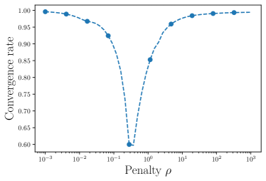
Figure 2: Empirical convergence rate of Fed-PLT for different values of $\rho$, and ${N_{\mathrm{e}}}=10$.

In Figure 3 we plot the rate obtained setting $\rho=0.3$ and varying the number of local epochs ${N_{\mathrm{e}}}$ from $1$ to $50$. Interestingly, the rate is not a monotonically decreasing function of ${N_{\mathrm{e}}}$. Rather, the rate decreases to a minimum for ${N_{\mathrm{e}}}\approx 10$, and then increases again, settling on a constant value for ${N_{\mathrm{e}}}>20$. Further simulations show that such rate is constant for all values ${N_{\mathrm{e}}}>20$ and very close to the rate $\zeta$ of the exact PRS (where ${N_{\mathrm{e}}}\to\infty$). Therefore, it appears that the use of an inexact proximal computation during local training can improve the speed of convergence. Quantifying this speed-up from a theoretical perspective is an interesting direction for future research.

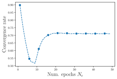
Figure 3: Empirical convergence rate of Fed-PLT for different numbers of local epochs, and $\rho=0.3$.

We conclude by remarking that these results lend further credence to the fact that the convergence rate of Fed-PLT is dominated by $\zeta$ rather than by the local training solver. Indeed, as observed Figure 2 resembles the rate of the exact PRS, and in Figure 3 the rate is very close to $\zeta$ even for small values of ${N_{\mathrm{e}}}\approx 20$.

Lemma 7 (Contraction of accelerated gradient).

Let $f\in\mathcal{F}_{{\underline{\lambda}},{\bar{\lambda}}}\left(\mathbb{R}^{n}\right)$, then the accelerated gradient descent

$$\mathbold{x}^{\ell+1} =\mathbold{w}^{\ell}-\frac{1}{{\bar{\lambda}}}\nabla f(\mathbold{w}^{\ell})$$

$$\mathbold{w}^{\ell+1} =\mathbold{x}^{\ell+1}+\frac{\sqrt{{\bar{\lambda}}}-\sqrt{{\underline{\lambda}}}}{\sqrt{{\bar{\lambda}}}+\sqrt{{\underline{\lambda}}}}(\mathbold{x}^{\ell+1}-\mathbold{x}^{\ell})$$

with initial conditions $\mathbold{x}^{0}=\mathbold{w}^{0}$ is such that

$$\left\lVert\mathbold{x}^{\ell}-\bar{\mathbold{x}}\right\rVert\leq\left(1+{\bar{\lambda}}/{\underline{\lambda}}\right)\left(1-\sqrt{{\underline{\lambda}}/{\bar{\lambda}}}\right)^{\ell}\left\lVert\mathbold{x}^{0}-\bar{\mathbold{x}}\right\rVert$$

where $\bar{\mathbold{x}}$ is the unique minimum of $f$. Therefore,

$$\ell>\frac{\log(1+{\bar{\lambda}}/{\underline{\lambda}})}{|\log(1-\sqrt{{\underline{\lambda}}/{\bar{\lambda}}})|}$$

is a sufficient condition for the accelerated gradient to be contractive.

Proof.

Define $\phi^{\ell}=f(\mathbold{x}^{\ell})-f(\bar{\mathbold{x}})+\frac{{\underline{\lambda}}}{2}\left\lVert\mathbold{w}^{\ell}-\bar{\mathbold{x}}\right\rVert^{2},$ then by [41, Theorem 4.14] we have that $\phi^{\ell+1}\leq\zeta\phi^{\ell}$ with $\zeta=1-\sqrt{{\underline{\lambda}}/{\bar{\lambda}}}$. Now, by smoothness of $f$ and the fact that $\nabla f(\bar{\mathbold{x}})$ we have $f(\mathbold{x}^{0})-f(\bar{\mathbold{x}})\leq({\bar{\lambda}}/2)\left\lVert\mathbold{x}^{0}-\bar{\mathbold{x}}\right\rVert^{2}$, which implies

$$\phi^{0}\leq\frac{{\bar{\lambda}}+{\underline{\lambda}}}{2}\left\lVert\mathbold{w}^{0}-\bar{\mathbold{x}}\right\rVert^{2}.$$

Therefore, using $\phi^{\ell+1}\leq\zeta\phi^{\ell}$ recursively we get

$$\phi^{\ell}\leq\zeta^{\ell}\phi^{0}\leq\frac{{\bar{\lambda}}+{\underline{\lambda}}}{2}\left\lVert\mathbold{w}^{0}-\bar{\mathbold{x}}\right\rVert^{2}$$

and, together with the fact $({\underline{\lambda}}/2)\left\lVert\mathbold{w}^{\ell}-\bar{\mathbold{x}}\right\rVert^{2}\leq\phi^{\ell}$ (which holds by definition of $\phi^{\ell}$), the thesis follows. The algorithm is then contractive w.r.t. $\mathbold{x}$ whenever a suitably large $\ell$ is chosen. ∎

References

- [1] T. Li, A. K. Sahu, A. Talwalkar, and V. Smith, “Federated Learning: Challenges, Methods, and Future Directions,” IEEE Signal Processing Magazine, vol. 37, pp. 50–60, May 2020.
- [2] C. Zhang, Y. Xie, H. Bai, B. Yu, W. Li, and Y. Gao, “A survey on federated learning,” Knowledge-Based Systems, vol. 216, p. 106775, Mar. 2021.
- [3] T. Gafni, N. Shlezinger, K. Cohen, Y. C. Eldar, and H. V. Poor, “Federated Learning: A signal processing perspective,” IEEE Signal Processing Magazine, vol. 39, pp. 14–41, May 2022.
- [4] A. Rauniyar, D. H. Hagos, D. Jha, J. E. Håkegård, U. Bagci, D. B. Rawat, and V. Vlassov, “Federated Learning for Medical Applications: A Taxonomy, Current Trends, Challenges, and Future Research Directions,” IEEE Internet of Things Journal, pp. 1–1, 2023.
- [5] L. Qian, P. Yang, M. Xiao, O. A. Dobre, M. D. Renzo, J. Li, Z. Han, Q. Yi, and J. Zhao, “Distributed Learning for Wireless Communications: Methods, Applications and Challenges,” IEEE Journal of Selected Topics in Signal Processing, vol. 16, pp. 326–342, Apr. 2022.
- [6] L. Li, Y. Fan, M. Tse, and K.-Y. Lin, “A review of applications in federated learning,” Computers & Industrial Engineering, vol. 149, p. 106854, Nov. 2020.
- [7] X. Cheng, C. Li, and X. Liu, “A Review of Federated Learning in Energy Systems,” in 2022 IEEE/IAS Industrial and Commercial Power System Asia (I&CPS Asia), (Shanghai, China), pp. 2089–2095, IEEE, July 2022.
- [8] S. Zhang, J. Li, L. Shi, M. Ding, D. C. Nguyen, W. Tan, J. Weng, and Z. Han, “Federated Learning in Intelligent Transportation Systems: Recent Applications and Open Problems,” IEEE Transactions on Intelligent Transportation Systems, pp. 1–27, 2024.
- [9] M. Nasr, R. Shokri, and A. Houmansadr, “Comprehensive privacy analysis of deep learning: Passive and active white-box inference attacks against centralized and federated learning,” in 2019 IEEE symposium on security and privacy (SP), pp. 739–753, IEEE, 2019.
- [10] R. Bassily, A. Smith, and A. Thakurta, “Private empirical risk minimization: Efficient algorithms and tight error bounds,” in 2014 IEEE 55th Annual Symposium on Foundations of Computer Science, pp. 464–473, IEEE, 2014.
- [11] R. Shokri, M. Stronati, C. Song, and V. Shmatikov, “Membership inference attacks against machine learning models,” in 2017 IEEE symposium on security and privacy (SP), pp. 3–18, IEEE, 2017.
- [12] A. M. Girgis, D. Data, S. Diggavi, P. Kairouz, and A. T. Suresh, “Shuffled model of federated learning: Privacy, accuracy and communication trade-offs,” IEEE journal on selected areas in information theory, vol. 2, no. 1, pp. 464–478, 2021.
- [13] G. D. Németh, M. A. Lozano, N. Quadrianto, and N. M. Oliver, “A Snapshot of the Frontiers of Client Selection in Federated Learning,” Transactions on Machine Learning Research, 2022.
- [14] M. Grudzień, G. Malinovsky, and P. Richtarik, “Can 5th Generation Local Training Methods Support Client Sampling? Yes!,” in Proceedings of The 26th International Conference on Artificial Intelligence and Statistics (F. Ruiz, J. Dy, and J.-W. van de Meent, eds.), vol. 206 of Proceedings of Machine Learning Research, pp. 1055–1092, PMLR, Apr. 2023.
- [15] Z. Zhao, Y. Mao, Y. Liu, L. Song, Y. Ouyang, X. Chen, and W. Ding, “Towards efficient communications in federated learning: A contemporary survey,” Journal of the Franklin Institute, p. S0016003222009346, Jan. 2023.
- [16] H. H. Bauschke and P. L. Combettes, Convex analysis and monotone operator theory in Hilbert spaces. CMS books in mathematics, Cham: Springer, 2 ed., 2017.
- [17] C. Zhang, S. Li, J. Xia, W. Wang, F. Yan, and Y. Liu, “BatchCrypt: Efficient homomorphic encryption for Cross-Silo federated learning,” in 2020 USENIX annual technical conference (USENIX ATC 20), pp. 493–506, 2020.
- [18] S. Zhang, T. O. Timoudas, and M. Dahleh, “Network consensus with privacy: A secret sharing method,” arXiv preprint arXiv:2103.03432, 2021.
- [19] C. Dwork, A. Roth, et al., “The algorithmic foundations of differential privacy,” Foundations and Trends® in Theoretical Computer Science, vol. 9, no. 3–4, pp. 211–407, 2014.
- [20] R. Chourasia, J. Ye, and R. Shokri, “Differential privacy dynamics of langevin diffusion and noisy gradient descent,” Advances in Neural Information Processing Systems, vol. 34, pp. 14771–14781, 2021.
- [21] K. Chaudhuri, C. Monteleoni, and A. D. Sarwate, “Differentially private empirical risk minimization,” Journal of Machine Learning Research, vol. 12, no. 3, 2011.
- [22] S. Amiri, A. Belloum, S. Klous, and L. Gommans, “Compressive differentially private federated learning through universal vector quantization,” in AAAI Workshop on Privacy-Preserving Artificial Intelligence, pp. 2–9, 2021.
- [23] K. Chaudhuri, C. Guo, and M. Rabbat, “Privacy-aware compression for federated data analysis,” in Proceedings of the Thirty-Eighth Conference on Uncertainty in Artificial Intelligence (J. Cussens and K. Zhang, eds.), vol. 180 of Proceedings of Machine Learning Research, pp. 296–306, PMLR, 01–05 Aug 2022.
- [24] N. Lang, E. Sofer, T. Shaked, and N. Shlezinger, “Joint Privacy Enhancement and Quantization in Federated Learning,” IEEE Transactions on Signal Processing, vol. 71, pp. 295–310, 2023.
- [25] S. Han, U. Topcu, and G. J. Pappas, “Differentially Private Distributed Constrained Optimization,” IEEE Transactions on Automatic Control, vol. 62, pp. 50–64, Jan. 2017.
- [26] S. Han and G. J. Pappas, “Privacy in Control and Dynamical Systems,” Annual Review of Control, Robotics, and Autonomous Systems, vol. 1, pp. 309–332, May 2018.
- [27] J. Le Ny and G. J. Pappas, “Differentially Private Filtering,” IEEE Transactions on Automatic Control, vol. 59, pp. 341–354, Feb. 2014.
- [28] J. Wang, J. Ke, and J.-F. Zhang, “Differentially private bipartite consensus over signed networks with time-varying noises,” IEEE Transactions on Automatic Control, 2024.
- [29] X. Zhang, M. Hong, S. Dhople, W. Yin, and Y. Liu, “FedPD: A Federated Learning Framework With Adaptivity to Non-IID Data,” IEEE Transactions on Signal Processing, vol. 69, pp. 6055–6070, 2021.
- [30] A. Mitra, R. Jaafar, G. J. Pappas, and H. Hassani, “Linear Convergence in Federated Learning: Tackling Client Heterogeneity and Sparse Gradients,” in Advances in Neural Information Processing Systems (M. Ranzato, A. Beygelzimer, Y. Dauphin, P. S. Liang, and J. W. Vaughan, eds.), vol. 34, pp. 14606–14619, Curran Associates, Inc., 2021.
- [31] L. Condat, I. Agarský, G. Malinovsky, and P. Richtárik, “TAMUNA: Doubly Accelerated Federated Learning with Local Training, Compression, and Partial Participation,” May 2023.
- [32] S. A. Alghunaim, “Local Exact-Diffusion for Decentralized Optimization and Learning,” Feb. 2023.
- [33] E. K. Ryu and S. Boyd, “A primer on monotone operator methods,” Applied and Computational Mathematics, vol. 15, no. 1, pp. 3–43, 2016.
- [34] N. Parikh and S. Boyd, “Proximal Algorithms,” Foundations and Trends® in Optimization, vol. 1, no. 3, pp. 127–239, 2014.
- [35] P. Giselsson and S. Boyd, “Linear Convergence and Metric Selection for Douglas-Rachford Splitting and ADMM,” IEEE Transactions on Automatic Control, vol. 62, pp. 532–544, Feb. 2017.
- [36] E. Gorbunov, F. Hanzely, and P. Richtarik, “A Unified Theory of SGD: Variance Reduction, Sampling, Quantization and Coordinate Descent,” in Proceedings of the Twenty Third International Conference on Artificial Intelligence and Statistics (S. Chiappa and R. Calandra, eds.), vol. 108 of Proceedings of Machine Learning Research, pp. 680–690, PMLR, Aug. 2020.
- [37] Z. Peng, T. Wu, Y. Xu, M. Yan, and W. Yin, “Coordinate Friendly Structures, Algorithms and Applications,” Annals of Mathematical Sciences and Applications, vol. 1, no. 1, pp. 57–119, 2016.
- [38] N. Bastianello, L. Madden, R. Carli, and E. Dall’Anese, “A Stochastic Operator Framework for Static and Online Optimization with Sub-Weibull Errors,” Aug. 2022.
- [39] I. Mironov, “Rényi differential privacy,” in 2017 IEEE 30th computer security foundations symposium (CSF), pp. 263–275, IEEE, 2017.
- [40] C. Liu, K. H. Johansson, and Y. Shi, “Distributed empirical risk minimization with differential privacy,” Automatica, vol. 162, p. 111514, 2024.
- [41] A. d’Aspremont, D. Scieur, and A. Taylor, “Acceleration Methods,” Foundations and Trends® in Optimization, vol. 5, no. 1-2, pp. 1–245, 2021.
- [42] J. Altschuler and K. Talwar, “Privacy of noisy stochastic gradient descent: More iterations without more privacy loss,” Advances in Neural Information Processing Systems, vol. 35, pp. 3788–3800, 2022.
- [43] Z. Li, W. Shi, and M. Yan, “A Decentralized Proximal-Gradient Method With Network Independent Step-Sizes and Separated Convergence Rates,” IEEE Transactions on Signal Processing, vol. 67, pp. 4494–4506, Sept. 2019.
- [44] A. L. Dončev and R. T. Rockafellar, Implicit functions and solution mappings: a view from variational analysis. Springer series in operations research and financial engineering, New York, NY Heidelberg Dordrecht: Springer, 2 ed., 2014.
- [45] H. H. Bauschke, S. M. Moffat, and X. Wang, “Firmly Nonexpansive Mappings and Maximally Monotone Operators: Correspondence and Duality,” Set-Valued and Variational Analysis, vol. 20, pp. 131–153, Mar. 2012.
- [46] G. Andrew, O. Thakkar, B. McMahan, and S. Ramaswamy, “Differentially private learning with adaptive clipping,” Advances in Neural Information Processing Systems, vol. 34, pp. 17455–17466, 2021.
- [47] T. Van Erven and P. Harremos, “Rényi divergence and kullback-leibler divergence,” IEEE Transactions on Information Theory, vol. 60, no. 7, pp. 3797–3820, 2014.
- [48] P. Kairouz, S. Oh, and P. Viswanath, “The composition theorem for differential privacy,” in International conference on machine learning, pp. 1376–1385, PMLR, 2015.
- [49] V. Feldman, I. Mironov, K. Talwar, and A. Thakurta, “Privacy amplification by iteration,” in 2018 IEEE 59th Annual Symposium on Foundations of Computer Science (FOCS), pp. 521–532, IEEE, 2018.
- [50] N. Bastianello and E. Dall’Anese, “Distributed and Inexact Proximal Gradient Method for Online Convex Optimization,” in 2021 European Control Conference (ECC), (Delft, Netherlands), pp. 2432–2437, 2021.
- [51] N. Bastianello, “tvopt: A Python Framework for Time-Varying Optimization,” in 2021 60th IEEE Conference on Decision and Control (CDC), pp. 227–232, 2021.
- [52] N. Bastianello, R. Carli, L. Schenato, and M. Todescato, “Asynchronous Distributed Optimization Over Lossy Networks via Relaxed ADMM: Stability and Linear Convergence,” IEEE Transactions on Automatic Control, vol. 66, pp. 2620–2635, June 2021.
- [53] E. K. Ryu, A. B. Taylor, C. Bergeling, and P. Giselsson, “Operator Splitting Performance Estimation: Tight Contraction Factors and Optimal Parameter Selection,” SIAM Journal on Optimization, vol. 30, pp. 2251–2271, Jan. 2020.