1 Introduction

The dispersive treatment of final-state interactions in three-body decays of mesons was originally introduced in refs. [1] and [2] in order to describe the observed deviation from a constant of the three-pion decay amplitudes of the charged kaons. This formalism was subsequently further studied, improved and developed by various authors, see refs. [3, 4, 5, 6, 7, 8, 9, 10] for a representative but incomplete list. Additional references and an informative account can be found in [11]. Although the early literature was mainly motivated by the description of $\pi\pi$ rescattering in the $K\to\pi\pi\pi$ amplitudes [1, 2, 4, 10], the more recent works were rather devoted to the three-pion decay of the eta meson [12, 13, 14, 15, 16, 17, 18]. But dispersive approaches of this Omnès-Khuri-Treiman-Sawyer-Wali type were also devised in a variety of other contexts, see for instance the articles [19, 20, 21, 22, 23, 24, 25, 26] for a sample of examples and for further references. Interestingly enough, the $K\to\pi\pi\pi$ transitions were not part of the more recent surge of interest for this kind of dispersive approach.

The main motivation for the present work, however, is not to simply fill this gap. It rather takes its origin in the observation that the amplitudes for the $K\to\pi\pi\pi$ transitions also enter the theoretical studies of the amplitudes of a certain number of rare decay modes of the kaons, like $K_{L}\to\pi^{0}\gamma\gamma$, $K_{L}\to\pi^{0}\gamma\ell^{+}\ell^{-}$, $K^{\pm}\to\pi^{\pm}\gamma\gamma$, $K\to\pi\ell^{+}\ell^{-}$, or $K^{\pm}\to\pi^{\pm}\gamma e^{+}e^{-}$, when considered from the point of view of the low-energy expansion. For these amplitudes, the lowest-order contribution starts at the one-loop level, with a pion loop rescattering into the leptonic/photonic component of the final state and originating from a tree-level $K\pi\pi\pi$ vertex. The latter is described by the two low-energy constants that also give the tree-level contribution to the $K\to\pi\pi$ amplitudes [27, 28]. However, most of the time these one-loop amplitudes do not provide a sufficiently accurate description of experimental data, and higher-order effects need to be included. In order to bypass a full-fledged two-loop calculation, the corrections that are applied to these amplitudes often amount, among other things, to the replacement of the two couplings entering the description of the $K\pi\pi\pi$ vertex at lowest order by appropriate combinations of parameters extracted from the phenomenological study of the experimental Dalitz plots of the $K\to\pi\pi\pi$ decays [29, 27, 28, 30]. For the amplitudes listed above, a procedure of this type was implemented in the articles [31, 32, 33], [34, 35], [36], [37], and [38], respectively. With the recent increase of precision in the experimental measurements of some of these processes, and with further improvements on the experimental side to be expected in the future [39, 40, 41, 42], these simple unitarization procedures, as they are often presented, might no longer be sufficient for an appropriate description of the data. Having at disposal a more solid description of final-state interactions in the $K\pi\to\pi\pi$ amplitudes constitutes a first step toward improving the situation on the theoretical side. The purpose of the present article is to construct and to provide such a tool. The subsequent applications to specific radiative kaon-decay amplitudes will, however, not be considered here and will be left for future studies.

On the practical side, our study will be performed under similar conditions as in refs. [1, 2], in the sense that CP-violating and isospin-breaking effects will be ignored. But in contrast to these references we will include both S- and P-wave contributions to the final-state rescattering of pion pairs, as done routinely in more recent studies, assuming that the contributions from higher partial waves to the absorptive parts can be neglected, at least in the range of energies where the resulting expressions can be applied. From this point of view, the general framework is quite similar to the one currently considered in the study of final-state interactions in the decay of the eta meson into three pions [12, 13, 14, 15, 16, 17, 18]. The main difference lies in the fact that the number of amplitudes to start with is somewhat larger in the case of the kaons, which can be charged or neutral. This is even more so the case to the extent that we will consider both the $\Delta I=1/2$ and $\Delta I=3/2$ components of the amplitudes. Fortunately, these can (and will of course) be treated separately.

The remainder of this article is organized in the following manner. In section 2 the set of initial 13 independent amplitudes is expressed in terms of nine isospin amplitudes. Crossing properties further reduce this set to only four independent amplitudes. In section 3 the isospin amplitudes are decomposed into single-variable functions. The polynomial ambiguities of this decomposition are discussed and, with a choice of appropriate asymptotic conditions, dispersion relations obeyed by the single-variable functions are obtained. The corresponding absorptive parts as provided by elastic unitarity are the subject of section 4. The final set of coupled Omnès-Khuri-Treiman dispersion relations for the single-variable functions are established in section 5, where their iterative numerical solution is also provided. Section 6 discusses the determination of the subtraction constants and considers two applications of the formalism: the description of the amplitudes as second-order polynomials in the Dalitz-plot variables, and the evaluation of the strong phases of the amplitudes for the decay modes of the charged kaon over the decay region. A summary and a few conclusions form the content of section 7. In order not to interrupt the narrative of the main text too frequently with issues and asides of a more technical kind, details related to several specific aspects that are only briefly discussed or mentioned in the bulk of the article have been gathered in a series of appendices.

2 Isospin and crossing properties of the $K\pi\to\pi\pi$ amplitudes

We start from the amplitudes for the processes $K^{+}(p_{K})\pi(p_{3})\to\pi(p_{1})\pi(p_{2})$ and $K^{0}(p_{K})\pi(p_{3})\to\pi(p_{1})\pi(p_{2})$ with all possible assignments of pion charges compatible with the conservation of the electric charge, and with all possible pion permutations. This gives altogether 13 amplitudes ${\cal A}_{i}(s,t,u)$, $i=1,\ldots,13$, with the labels chosen as indicated in Table 1. Since violation of CP symmetry is not important for the present study, we assume CP to be conserved. We thus need not consider explicitly the $K\pi\to\pi\pi$ amplitudes involving $K^{-}$ or ${\bar{K}}^{0}$, since they can be obtained as CP conjugate of those involving $K^{+}$ or $K^{0}$, respectively. The Mandelstam variables are defined as usual,

$$s=(p_{K}+p_{3})^{2},\quad t=(p_{K}-p_{1})^{2},\quad u=(p_{K}-p_{2})^{2}.$$ (2.1)

The amplitudes for the decay processes $K\to\pi\pi\pi$ are obtained from the previous ones through crossing, and are usually expressed in terms of the variables $s_{i}=(p_{K}-p_{i})^{2}$, $i=1,2,3$. In either case, one has $s+t+u=3s_{0}$ or $s_{1}+s_{2}+s_{3}=3s_{0}$, with

$$s_{0}=M_{\pi}^{2}+M_{K}^{2}/3.$$ (2.2)

We also assume isospin to be conserved, so that charged and neutral kaons (pions) share the same mass $M_{K}$ ($M_{\pi}$). For numerical applications, we take for the value of $M_{\pi}$ the mass of the charged pion, and for $M_{K}$ the average of the masses of the neutral and charged kaons. With the values provided by the Review of Particle Properties [45] this means

$$M_{\pi}=0.13957039~{}{\rm GeV},\quad M_{K}=0.495644~{}{\rm GeV}.$$ (2.3)

The phases inside a given isospin multiplet, i.e. either $(K^{0},K^{+})$ or $(\pi^{-},\pi^{0},\pi^{+})$, are chosen according to the Condon and Shortley convention [46]. Phases between these two isospin multiplets are set according to the prescription of de Swart [47]. These choices explain the crossing phases displayed in the two last columns of Table 1. Each initial $K\pi$ state is therefore characterized by its total isospin projection ${\cal I}_{z}$. Likewise, the final $\pi\pi$ states have total isospin projections $I_{z}$. These values are given in the third and fourth columns of Table 1, respectively. As to the total isospin, it can take the values ${\cal I}=\frac{1}{2},\frac{3}{2}$ for the $K\pi$ states or $I=0,1,2$ for the two-pion states.

The crossing properties and isospin symmetry will reduce the number of independent amplitudes. Crossing will only operate among subsets of amplitudes separated by the horizontal lines in Table 1. Constraints involving amplitudes that belong to different subsets will only occur through the implementation of isospin symmetry. In order to achieve this, we need to specify the symmetry properties of the operators that are responsible for the $K\pi\to\pi\pi$ transitions. As is well known, at first order in the Fermi constant, and in the absence of electroweak corrections (required by our assumption that isospin is conserved) these transitions are described by matrix elements

$$\langle\pi\pi|{\rm T}^{\Delta S=1}|K\pi\rangle,$$ (2.4)

where ${\rm T}^{\Delta S=1}$ is given by the integral of the effective Lagrangian for weak non-leptonic $\Delta S=1$ transitions [48, 49, 50, 51, 52, 53]. What matters here is that ${\rm T}^{\Delta S=1}$ proceeds by either $\Delta I=\frac{1}{2}$ or $\Delta I=\frac{3}{2}$ isospin transitions,

$${\rm T}^{\Delta S=1}={\rm T}^{\frac{1}{2}}_{\frac{1}{2}}+{\rm T}^{\frac{3}{2}}_{\frac{1}{2}},$$ (2.5)

where the superscript gives the total isospin $\Delta I$ and the subscript the corresponding isospin projection, which is necessarily $\frac{1}{2}$. In order to simplify the notation, we will omit this subscript in the sequel. Upon expanding the $|K\pi\rangle$ and $|\pi\pi\rangle$ states over isospin states $|{\cal I},{\cal I}_{z}\rangle$ and $|I,I_{z}\rangle$, respectively, we can implement the Wigner-Eckart theorem and express each transition amplitude in terms of a small number of reduced matrix elements, multiplied by the appropriate Clebsch-Gordan coefficients,

$$\langle I,I_{z}|{\rm T}^{\frac{1}{2}}|{\cal I},{\cal I}_{z}\rangle=\Big{(}{\cal I},{\cal I}_{z};\frac{1}{2},\frac{1}{2}\Big{|}I,I_{z}\Big{)}\langle I|\!|{\rm T}^{\frac{1}{2}}|\!|{\cal I}\rangle,~{}~{}\langle I,I_{z}|{\rm T}^{\frac{3}{2}}|{\cal I},{\cal I}_{z}\rangle=\Big{(}{\cal I},{\cal I}_{z};\frac{3}{2},\frac{1}{2}\Big{|}I,I_{z}\Big{)}\langle I|\!|{\rm T}^{\frac{3}{2}}|\!|{\cal I}\rangle.$$ (2.6)

With the phase convention adopted here, the Clebsch-Gordan coefficients can be read off, for instance, from the tables provided in ref. [45].

$i$	reaction	${\cal I}_{z}$	$I_{z}$	$t\leftrightarrow u$	$s\leftrightarrow t$	$u\leftrightarrow s$
1	$K^{+}\pi^{+}\to\pi^{+}\pi^{+}$	$+\frac{3}{2}$	$\!\!{+2}$	1	3	2
2	$K^{+}\pi^{-}\to\pi^{+}\pi^{-}$	$-\frac{1}{2}$	$~{}0$	3	2	1
3	$K^{+}\pi^{-}\to\pi^{-}\pi^{+}$	$-\frac{1}{2}$	$~{}0$	2	1	3
4	$K^{+}\pi^{-}\to\pi^{0}\pi^{0}$	$-\frac{1}{2}$	$~{}0$	4	$\!\!\!\!{-6}$	$\!\!\!\!{-5}$
5	$K^{+}\pi^{0}\to\pi^{0}\pi^{+}$	$+\frac{1}{2}$	$\!\!{+1}$	6	5	$\!\!\!\!{-4}$
6	$K^{+}\pi^{0}\to\pi^{+}\pi^{0}$	$+\frac{1}{2}$	$\!\!{+1}$	5	$\!\!\!\!{-4}$	6
7	$K^{0}\pi^{0}\to\pi^{+}\pi^{-}$	$-\frac{1}{2}$	$~{}0$	8	$\!\!\!\!\!{-12}$	$\!\!\!\!{-9}$
8	$K^{0}\pi^{0}\to\pi^{-}\pi^{+}$	$-\frac{1}{2}$	$~{}0$	7	$\!\!\!\!\!{-10}$	$\!\!\!\!\!{-11}$
9	$K^{0}\pi^{+}\to\pi^{+}\pi^{0}$	$+\frac{1}{2}$	$\!\!{+1}$	$\!\!{10}$	$\!{11}$	$\!\!\!\!{-7}$
$\!\!{10}$	$K^{0}\pi^{+}\to\pi^{0}\pi^{+}$	$+\frac{1}{2}$	$\!\!{+1}$	9	$\!\!\!\!{-8}$	$\!\!{12}$
$\!\!{11}$	$K^{0}\pi^{-}\to\pi^{-}\pi^{0}$	$-\frac{3}{2}$	$\!\!{-1}$	$\!\!{12}$	9	$\!\!\!\!{-8}$
$\!\!{12}$	$K^{0}\pi^{-}\to\pi^{0}\pi^{-}$	$-\frac{3}{2}$	$\!\!{-1}$	$\!\!{11}$	$\!\!\!\!{-7}$	$\!\!{10}$
$\!\!{13}$	$K^{0}\pi^{0}\to\pi^{0}\pi^{0}$	$-\frac{1}{2}$	$~{}0$	$\!\!{13}$	$\!\!{13}$	$\!\!{13}$

Table 1: The 13 amplitudes ${\cal A}_{i}(s,t,u)$ with the corresponding isospin projections ${\cal I}_{z}$ and $I_{z}$ of the $K\pi$ and $\pi\pi$ pairs, respectively. The first column gives the label $i$ assigned to the amplitude that describes the process displayed in the second column. The crossing properties of the amplitudes are also indicated in the last three columns. These entries should be read, for instance, as follows: ${\cal A}_{1}(t,s,u)=+{\cal A}_{3}(s,t,u)$ or ${\cal A}_{4}(u,t,s)=-{\cal A}_{5}(t,s,u)$. The horizontal lines delimit subsets of amplitudes that are closed under crossing.

There are four independent reduced amplitudes of the type $\langle I|\!|{\rm T}^{\frac{1}{2}}|\!|{\cal I}\rangle(s,t,u)$, and five of the type $\langle I|\!|{\rm T}^{\frac{3}{2}}|\!|{\cal I}\rangle(s,t,u)$. For reasons of convenience, we will work with the isospin amplitudes ${\cal M}_{1}^{I;{\cal I}}(s,t,u)$, defined as

$${\vec{\cal M}}_{1}(s,t,u)\equiv\left(\!\!\!\begin{tabular}[]{c}${\cal M}_{1}^{2;\frac{3}{2}}(s,t,u)$\\ ${\cal M}_{1}^{1;\frac{3}{2}}(s,t,u)$\\ ${\cal M}_{1}^{1;\frac{1}{2}}(s,t,u)$\\ ${\cal M}_{1}^{0;\frac{1}{2}}(s,t,u)$\end{tabular}\!\!\!\right)=\left(\!\!\begin{tabular}[]{cccc}$1$&0&0&0\\ 0&$-\sqrt{3}$&0&0\\ 0&0&$\sqrt{\frac{3}{2}}$&0\\ 0&0&0&$-1$\end{tabular}\!\!\right)\left(\!\!\!\begin{tabular}[]{c}$\langle 2|\!|{\rm T}^{\frac{1}{2}}|\!|\frac{3}{2}\rangle(s,t,u)$\\ $\langle 1|\!|{\rm T}^{\frac{1}{2}}|\!|\frac{3}{2}\rangle(s,t,u)$\\ $\langle 1|\!|{\rm T}^{\frac{1}{2}}|\!|\frac{1}{2}\rangle(s,t,u)$\\ $\langle 0|\!|{\rm T}^{\frac{1}{2}}|\!|\frac{1}{2}\rangle(s,t,u)$\end{tabular}\!\!\!\right),$$ (2.7)

for the $\Delta I=\frac{1}{2}$ transitions, and, for the $\Delta I=\frac{3}{2}$ transitions, with the isospin amplitudes ${\cal M}_{3}^{I;{\cal I}}(s,t,u)$, where

$${\vec{\cal M}}_{3}(s,t,u)\equiv\left(\!\!\!\begin{tabular}[]{c}${\cal M}_{3}^{2;\frac{3}{2}}(s,t,u)$\\ ${\cal M}_{3}^{2;\frac{1}{2}}(s,t,u)$\\ ${\cal M}_{3}^{1;\frac{3}{2}}(s,t,u)$\\ ${\cal M}_{3}^{1;\frac{1}{2}}(s,t,u)$\\ ${\cal M}_{3}^{0;\frac{3}{2}}(s,t,u)$\end{tabular}\!\!\!\right)=\left(\!\!\begin{tabular}[]{ccccc}$\frac{1}{\sqrt{2}}$&0&0&0&0\\ 0&$\frac{1}{\sqrt{2}}$&0&0&0\\ 0&0&$-\sqrt{\frac{3}{10}}$&0&0\\ 0&0&0&$-\sqrt{\frac{3}{2}}$&0\\ 0&0&0&0&$\frac{1}{2}$\end{tabular}\!\!\right)\left(\!\!\!\begin{tabular}[]{c}$\langle 2|\!|{\rm T}^{\frac{3}{2}}|\!|\frac{3}{2}\rangle(s,t,u)$\\ $\langle 2|\!|{\rm T}^{\frac{3}{2}}|\!|\frac{1}{2}\rangle(s,t,u)$\\ $\langle 1|\!|{\rm T}^{\frac{3}{2}}|\!|\frac{3}{2}\rangle(s,t,u)$\\ $\langle 1|\!|{\rm T}^{\frac{3}{2}}|\!|\frac{1}{2}\rangle(s,t,u)$\\ $\langle 0|\!|{\rm T}^{\frac{3}{2}}|\!|\frac{3}{2}\rangle(s,t,u)$\end{tabular}\!\!\!\right).$$ (2.8)

In matrix notation, the relations between the 13 amplitudes ${\cal A}_{i}$ of Table 1 and these isospin amplitudes write as

$${\vec{\cal A}}(s,t,u)={\mathbf{R}}_{1}{\vec{\cal M}}_{1}(s,t,u)+{\mathbf{R}}_{3}{\vec{\cal M}}_{3}(s,t,u),$$ (2.9)

with the $4\times 13$ and $5\times 13$ matrices ${\mathbf{R}}_{1}$ and ${\mathbf{R}}_{3}$ given by

$${\mathbf{R}}_{1}=\left(\!\!\begin{tabular}[]{cccc}1&0&0&0\\ $\frac{1}{6}$&$\frac{1}{6}$&$\frac{1}{3}$&$\frac{1}{3}$\\[2.84544pt] $\frac{1}{6}$&$-\frac{1}{6}~{}~{}$&$-\frac{1}{3}~{}~{}$&$\frac{1}{3}$\\[2.84544pt] $\frac{1}{3}$&0&0&$-\frac{1}{3}~{}~{}$\\[2.84544pt] $\frac{1}{2}$&$-\frac{1}{6}~{}~{}$&$-\frac{1}{3}~{}~{}$&0\\[2.84544pt] $\frac{1}{2}$&$\frac{1}{6}$&$\frac{1}{3}$&0\\[4.26773pt] $\frac{1}{3\sqrt{2}}$&$\frac{1}{3\sqrt{2}}$&$-\frac{1}{3\sqrt{2}}~{}~{}$&$-\frac{1}{3\sqrt{2}}~{}~{}$\\[4.26773pt] $\frac{1}{3\sqrt{2}}$&$-\frac{1}{3\sqrt{2}}~{}~{}$&$\frac{1}{3\sqrt{2}}$&$-\frac{1}{3\sqrt{2}}~{}~{}$\\[4.26773pt] $\frac{1}{2\sqrt{2}}$&$\frac{1}{6\sqrt{2}}$&$-\frac{\sqrt{2}}{3}~{}~{}$&0\\[4.26773pt] $\frac{1}{2\sqrt{2}}$&$-\frac{1}{6\sqrt{2}}~{}~{}$&$\frac{\sqrt{2}}{3}$&0\\[4.26773pt] $\frac{1}{2\sqrt{2}}$&$-\frac{1}{2\sqrt{2}}~{}~{}$&0&0\\[4.26773pt] $\frac{1}{2\sqrt{2}}$&$\frac{1}{2\sqrt{2}}$&0&0\\[4.26773pt] $\frac{\sqrt{2}}{3}$&0&0&$\frac{1}{3\sqrt{2}}$\end{tabular}\!\!\!\right),~{}{\mathbf{R}}_{3}=\left(\!\!\begin{tabular}[]{ccccc}1&0&0&0&0\\ $-\frac{1}{6}~{}~{}$&$\frac{1}{3}$&$\frac{1}{6}$&$\frac{1}{3}$&$\frac{1}{3}$\\[2.84544pt] $-\frac{1}{6}~{}~{}$&$\frac{1}{3}$&$-\frac{1}{6}~{}~{}$&$-\frac{1}{3}~{}~{}$&$\frac{1}{3}$\\[2.84544pt] $-\frac{1}{3}~{}~{}$&$\frac{2}{3}$&0&0&$-\frac{1}{3}~{}~{}$\\[2.84544pt] 0&$\frac{1}{2}$&$-\frac{2}{3}~{}~{}$&$\frac{1}{6}$&0\\[2.84544pt] 0&$\frac{1}{2}$&$\frac{2}{3}$&$-\frac{1}{6}~{}~{}$&0\\[4.26773pt] $-\frac{1}{3\sqrt{2}}~{}~{}$&$-\frac{1}{3\sqrt{2}}~{}~{}$&$\frac{1}{3\sqrt{2}}$&$-\frac{1}{3\sqrt{2}}~{}~{}$&$\frac{\sqrt{2}}{3}$\\[4.26773pt] $-\frac{1}{3\sqrt{2}}~{}~{}$&$-\frac{1}{3\sqrt{2}}~{}~{}$&$-\frac{1}{3\sqrt{2}}~{}~{}$&$\frac{1}{3\sqrt{2}}$&$\frac{\sqrt{2}}{3}$\\[2.84544pt] 0&$-\frac{1}{\sqrt{2}}~{}~{}$&$\frac{\sqrt{2}}{3}$&$\frac{1}{3\sqrt{2}}$&0\\[2.84544pt] 0&$-\frac{1}{2\sqrt{2}}~{}~{}$&$-\frac{\sqrt{2}}{3}~{}~{}$&$-\frac{1}{3\sqrt{2}}~{}~{}$&0\\[2.84544pt] $-\frac{1}{\sqrt{2}}~{}~{}$&0&$\frac{1}{\sqrt{2}}$&0&0\\[4.26773pt] $-\frac{1}{\sqrt{2}}~{}~{}$&0&$-\frac{1}{\sqrt{2}}~{}~{}$&0&0\\[4.26773pt] $-\frac{\sqrt{2}}{3}~{}~{}$&$-\frac{\sqrt{2}}{3}~{}~{}$&0&0&$-\frac{\sqrt{2}}{3}~{}~{}$\end{tabular}\!\!\!\right).$$ (2.10)

The crossing relations among the isospin amplitudes follow from those among the amplitudes ${\cal A}_{i}(s,t,u)$, and express themselves in the form

$${\vec{\cal M}}_{1,3}(s,u,t)=C_{tu}^{(1,3)}{\vec{\cal M}}_{1,3}(s,t,u),\quad{\vec{\cal M}}_{1,3}(t,s,u)=C_{st}^{(1,3)}{\vec{\cal M}}_{1,3}(s,t,u),\quad{\vec{\cal M}}_{1,3}(u,t,s)=C_{us}^{(1,3)}{\vec{\cal M}}_{1,3}(s,t,u).$$ (2.11)

All six crossing matrices $C_{tu}^{(1,3)}$, $C_{st}^{(1,3)}$, $C_{us}^{(1,3)}$, must square to the unit matrix and satisfy, in addition,

$$C_{tu}^{(1,3)}C_{st}^{(1,3)}C_{tu}^{(1,3)}=C_{us}^{(1,3)}=C_{st}^{(1,3)}C_{tu}^{(1,3)}C_{st}^{(1,3)}.$$ (2.12)

One finds that the matrices $C_{tu}^{(1,3)}$ are diagonal,

$$C_{tu}^{(1)}={\rm diag}(+1,-1,-1,+1),~{}~{}C_{tu}^{(3)}={\rm diag}(+1,+1,-1,-1,+1),$$ (2.13)

whereas the remaining crossing matrices are given by

$$C_{st}^{(1)}=\left(\begin{tabular}[]{cccc}$+\frac{1}{6}$&$-\frac{1}{6}$&$-\frac{1}{3}$&$+\frac{1}{3}$\\[2.84544pt] $-\frac{5}{6}$&$-\frac{1}{2}$&$+1$&$+\frac{1}{3}$\\[2.84544pt] $-\frac{5}{6}$&$+\frac{1}{2}$&$~{}~{}0$&$+\frac{1}{3}$\\[2.84544pt] $+\frac{5}{3}$&$+\frac{1}{3}$&$+\frac{2}{3}$&$+\frac{1}{3}$\end{tabular}\right)\!,~{}~{}C_{us}^{(1)}=\left(\begin{tabular}[]{cccc}$+\frac{1}{6}$&$+\frac{1}{6}$&$+\frac{1}{3}$&$+\frac{1}{3}$\\[2.84544pt] $+\frac{5}{6}$&$-\frac{1}{2}$&$+1$&$-\frac{1}{3}$\\[2.84544pt] $+\frac{5}{6}$&$+\frac{1}{2}$&$~{}~{}0$&$-\frac{1}{3}$\\[2.84544pt] $+\frac{5}{3}$&$-\frac{1}{3}$&$-\frac{2}{3}$&$+\frac{1}{3}$\end{tabular}\right)\!,$$ (2.14)

and

$$C_{st}^{(3)}=\left(\begin{tabular}[]{ccccc}$-\frac{1}{6}$&$+\frac{1}{3}$&$-\frac{1}{6}$&$-\frac{1}{3}$&$+\frac{1}{3}$\\[2.84544pt] $+\frac{1}{3}$&$-\frac{1}{6}$&$-\frac{2}{3}$&$+\frac{1}{6}$&$+\frac{1}{3}$\\[2.84544pt] $-\frac{1}{6}$&$-\frac{2}{3}$&$+\frac{1}{2}$&$~{}~{}0$&$+\frac{1}{3}$\\[2.84544pt] $-\frac{5}{3}$&$+\frac{5}{6}$&$~{}~{}0$&$+\frac{1}{2}$&$+\frac{1}{3}$\\[2.84544pt] $+\frac{5}{6}$&$+\frac{5}{6}$&$+\frac{5}{6}$&$+\frac{1}{6}$&$+\frac{1}{3}$\end{tabular}\right)\!,~{}~{}C_{us}^{(3)}=\left(\begin{tabular}[]{ccccc}$-\frac{1}{6}$&$+\frac{1}{3}$&$+\frac{1}{6}$&$+\frac{1}{3}$&$+\frac{1}{3}$\\[2.84544pt] $+\frac{1}{3}$&$-\frac{1}{6}$&$+\frac{2}{3}$&$-\frac{1}{6}$&$+\frac{1}{3}$\\[2.84544pt] $+\frac{1}{6}$&$+\frac{2}{3}$&$+\frac{1}{2}$&$~{}~{}0$&$-\frac{1}{3}$\\[2.84544pt] $+\frac{5}{3}$&$-\frac{5}{6}$&$~{}~{}0$&$+\frac{1}{2}$&$-\frac{1}{3}$\\[2.84544pt] $+\frac{5}{6}$&$+\frac{5}{6}$&$-\frac{5}{6}$&$-\frac{1}{6}$&$+\frac{1}{3}$\end{tabular}\right)\!.$$ (2.15)

It is a straightforward exercise to check that these matrices indeed satisfy all the properties stated above. We will indicate a simple way to work out these crossing matrices at the end of this section, once we have introduced a representation of the isospin functions in terms of a more reduced set of independent amplitudes.

While the isospin amplitudes take into account the restrictions coming from isospin symmetry, they do not represent the most compact description of the amplitudes ${\cal A}_{i}(s,t,u)$, and one may expect that the number of independent functions that are required to this effect can be further reduced. This expectation is, for instance, borne out by the similar and well-known situation in the case of elastic pion-pion scattering in the absence of isospin-breaking effects. There are only three isospin amplitudes in that case, but once crossing is enforced, a single function $A(s|t,u)$, with $A(s|t,u)=A(s|u,t)$, is enough to describe the amplitudes of all the scattering channels [54, 55]. In the present case, one can indeed construct a representation of the isospin amplitudes in terms of only four independent functions, two in each of the two sectors, ${\cal M}_{1}$ and ${\cal N}_{1}$ in the $\Delta I=1/2$ sector, ${\cal M}_{3}$ and ${\cal N}_{3}$ in the $\Delta I=3/2$ sector. The details of this construction are given in appendix A, whereas appendix B provides, for the interested reader, an alternative derivation based on the so-called spurion formalism. Here we simply present the result of this analysis, which allows the isospin amplitudes to be expressed as

$${\cal M}^{2;\frac{3}{2}}_{1}(s,t,u) = {\cal M}_{1}(t|s,u)+{\cal M}_{1}(u|s,t),$$

$${\cal M}^{1;\frac{3}{2}}_{1}(s,t,u) = {\cal M}_{1}(t|s,u)-{\cal M}_{1}(u|s,t)-2{\cal N}_{1}(s,t,u),$$

$${\cal M}^{1;\frac{1}{2}}_{1}(s,t,u) = {\cal M}_{1}(t|s,u)-{\cal M}_{1}(u|s,t)+{\cal N}_{1}(s,t,u),$$

$${\cal M}^{0;\frac{1}{2}}_{1}(s,t,u) = 3{\cal M}_{1}(s|t,u)+{\cal M}_{1}(t|s,u)+{\cal M}_{1}(u|s,t),$$ (2.16)

and

$${\cal M}^{2;\frac{3}{2}}_{3}(s,t,u) = {\cal M}_{3}(t|s,u)+{\cal M}_{3}(u|s,t)+{\cal N}_{3}(t,s,u)+{\cal N}_{3}(u,s,t),$$

$${\cal M}^{2;\frac{1}{2}}_{3}(s,t,u) = {\cal M}_{3}(t|s,u)+{\cal M}_{3}(u|s,t),$$

$${\cal M}^{1;\frac{3}{2}}_{3}(s,t,u) = {\cal M}_{3}(t|s,u)-{\cal M}_{3}(u|s,t)-{\cal N}_{3}(s,t,u),$$

$${\cal M}^{1;\frac{1}{2}}_{3}(s,t,u) = {\cal M}_{3}(t|s,u)-{\cal M}_{3}(u|s,t)-4{\cal N}_{3}(s,t,u),$$

$${\cal M}^{0;\frac{3}{2}}_{3}(s,t,u) = 3\,{\cal M}_{3}(s|t,u)+{\cal M}_{3}(t|s,u)+{\cal M}_{3}(u|s,t)-{\cal N}_{3}(t,s,u)-{\cal N}_{3}(u,s,t),$$ (2.17)

where the following restrictions apply:

1. both functions ${\cal M}_{1}(s|t,u)$ and ${\cal M}_{3}(s|t,u)$ are symmetric under permutation of the variables $t$ and $u$;

2. the function ${\cal N}_{1}(s,t,u)$ is antisymmetric under permutation of any two of its variables;

3. the function ${\cal N}_{3}(s,t,u)$ is antisymmetric under permutation of the variables $t$ and $u$, and is in addition subject to the condition

   $${\cal N}_{3}(s,t,u)+{\cal N}_{3}(t,u,s)+{\cal N}_{3}(u,s,t)=0.$$ (2.18)

Notice that some of these symmetry properties reflect the fact that the amplitudes with $I=0$ or $I=2$ ($I=1$) will only produce partial-wave projections with even (odd) values of the total angular momentum, as required by Bose symmetry.

Coming now back to the crossing matrices introduced in eq. (2.11), one notices, for instance, that eq. (2.16) tells us that ${\cal M}^{2;\frac{3}{2}}_{1}(t,s,u)$ is equal to ${\cal M}_{1}(s|t,u)+{\cal M}_{1}(u|s,t)$. The two amplitudes in this sum can in turn be expressed in terms of the isospin amplitudes ${\cal M}_{1}^{I;{\cal I}}(s,t,u)$ upon inverting Eq. (2.16), giving

$${\cal M}^{2;\frac{3}{2}}_{1}(t,s,u)=\frac{1}{6}{\cal M}^{2;\frac{3}{2}}_{1}(s,t,u)-\frac{1}{6}{\cal M}^{1;\frac{3}{2}}_{1}(s,t,u)-\frac{1}{3}{\cal M}^{1;\frac{1}{2}}_{1}(s,t,u)+\frac{1}{3}{\cal M}^{0;\frac{1}{2}}_{1}(s,t,u).$$ (2.19)

Working out the other cases along similar lines, one easily reproduces the crossing matrices for the isospin amplitudes given in eqs. (2.14) and (2.15) above. This actually proves that the decompositions (2.16) and (2.17) are indeed compatible with the crossing properties of the amplitudes ${\vec{\cal A}}(s,t,u)$.

3 Representation of the amplitudes in terms of single-variable functions

3.1 Decomposition of the amplitudes into single-variable functions

On general grounds, we expect that the amplitudes ${\cal A}_{i}(s,t,u)$, or the isospin amplitudes ${\cal M}_{1,3}^{I;{\cal I}}(s,t,u)$ discussed in the previous section, satisfy fixed-$t$ dispersion relations. In order to set up a system of dispersion relations of the Khuri-Treiman type for, say, the isospin amplitudes, we need to express them in terms of a set of functions of a single variable. Such a representation will hold in the energy region where the absorptive parts of the partial waves with total angular momentum equal to or higher than two can be neglected in the dispersive integrals. Requiring that the resulting amplitudes also satisfy the appropriate crossing relations then leads to the expressions (numerical factors have been chosen for convenience)

$${\vec{\cal M}}_{1}(s,t,u)=\left(\begin{tabular}[]{c}$2M_{1}^{2;\frac{3}{2}}(s)$\\ $2(t-u)M_{1}^{1;\frac{3}{2}}(s)$\\ $2(t-u)M_{1}^{1;\frac{1}{2}}(s)$\\ $3M_{1}^{0;\frac{1}{2}}(s)$\end{tabular}\right)+C_{st}^{(1)}\left(\begin{tabular}[]{c}$2M_{1}^{2;\frac{3}{2}}(t)$\\ $2(s-u)M_{1}^{1;\frac{3}{2}}(t)$\\ $2(s-u)M_{1}^{1;\frac{1}{2}}(t)$\\ $3M_{1}^{0;\frac{1}{2}}(t)$\end{tabular}\right)+C_{tu}^{(1)}C_{st}^{(1)}\left(\begin{tabular}[]{c}$2M_{1}^{2;\frac{3}{2}}(u)$\\ $2(s-t)M_{1}^{1;\frac{3}{2}}(u)$\\ $2(s-t)M_{1}^{1;\frac{1}{2}}(u)$\\ $3M_{1}^{0;\frac{1}{2}}(u)$\end{tabular}\right)$$ (3.1)

and

$${\vec{\cal M}}_{3}(s,t,u)=\left(\begin{tabular}[]{c}$2M_{3}^{2;\frac{3}{2}}(s)$\\ $2M_{3}^{2;\frac{1}{2}}(s)$\\ $2(t-u)M_{3}^{1;\frac{3}{2}}(s)$\\ $2(t-u)M_{3}^{1;\frac{1}{2}}(s)$\\ $3M_{3}^{0;\frac{3}{2}}(s)$\end{tabular}\right)+C_{st}^{(3)}\left(\begin{tabular}[]{c}$2M_{3}^{2;\frac{3}{2}}(t)$\\ $2M_{3}^{2;\frac{1}{2}}(t)$\\ $2(s-u)M_{3}^{1;\frac{3}{2}}(t)$\\ $2(s-u)M_{3}^{2;\frac{1}{2}}(t)$\\ $3M_{3}^{0;\frac{3}{2}}(t)$\end{tabular}\right)+C_{tu}^{(3)}C_{st}^{(3)}\left(\begin{tabular}[]{c}$2M_{3}^{2;\frac{3}{2}}(u)$\\ $2M_{3}^{2;\frac{1}{2}}(u)$\\ $2(s-t)M_{3}^{1;\frac{3}{2}}(u)$\\ $2(s-t)M_{3}^{1;\frac{1}{2}}(u)$\\ $3M_{3}^{0;\frac{3}{2}}(u)$\end{tabular}\right)$$ (3.2)

The derivation of these representations, which has by now become standard and is amply documented in the existing literature, also shows that the functions of a single variable involved are analytic except for a right-hand cut starting at the two-pion threshold, with the discontinuity given by unitarity. Before constructing the corresponding dispersion relations, we need to give consideration to two issues. The first one concerns the non-unicity of the decomposition into single-variable functions. The second one concerns the asymptotic conditions that the amplitudes are required to satisfy. The remaining part of the present section will successively address these two aspects. We also briefly discuss the connection of the single-variable representations discussed here with other decompositions used in the literature.

3.2 Polynomial ambiguities

The decompositions of the amplitudes ${\cal A}_{i}(s,t,u)$ in terms of the single-variable functions $M_{1,3}^{I;{\cal I}}$, are unique only modulo some polynomials of finite degrees in $s$. In other words, alternative decompositions, in terms of functions ${\widetilde{M}}_{1,3}^{I;{\cal I}}(s)$, are possible, where the differences $\delta M_{1,3}^{I;{\cal I}}(s)\equiv{\widetilde{M}}_{1,3}^{I;{\cal I}}(s)-M_{1,3}^{I;{\cal I}}(s)$ are polynomials. In order to determine the most general form of the polynomials $\delta M_{1,3}^{I;{\cal I}}(s)$ one may easily adapt the method used in Ref. [16] to the case at hand. It is convenient, and equivalent, to discuss this issue at the level of the invariant functions ${\cal M}_{1,3}(s|t,u)$ and ${\cal N}_{1,3}(s,t,u)$. Inverting the relations (2.16) and (2.17) and replacing the isospin amplitudes by their expressions (3.1) and (3.2), one obtains

$${\cal M}_{1}(s|t,u) = M_{1}^{0;\frac{1}{2}}(s)-\frac{2}{3}M_{1}^{2;\frac{3}{2}}(s)+M_{1}^{2;\frac{3}{2}}(t)+M_{1}^{2;\frac{3}{2}}(u)$$

$$\!\!\!\!\!+\,\frac{1}{3}(s-u)\left[M_{1}^{1;\frac{3}{2}}(t)+2M_{1}^{1;\frac{1}{2}}(t)\right]+\frac{1}{3}(s-t)\left[M_{1}^{1;\frac{3}{2}}(u)+2M_{1}^{1;\frac{1}{2}}(u)\right],$$

$${\cal N}_{1}(s,t,u) = \frac{2}{3}(t-u)\left[M_{1}^{1;\frac{1}{2}}(s)-M_{1}^{1;\frac{3}{2}}(s)\right]+\frac{2}{3}(u-s)\left[M_{1}^{1;\frac{1}{2}}(t)-M_{1}^{1;\frac{3}{2}}(t)\right]$$

$$\!\!\!\!\!+\,\frac{2}{3}(s-t)\left[M_{1}^{1;\frac{1}{2}}(u)-M_{1}^{1;\frac{3}{2}}(u)\right],$$

$${\cal M}_{3}(s|t,u) = M_{3}^{0;\frac{3}{2}}(s)+\frac{2}{3}\left[M_{3}^{2;\frac{3}{2}}(s)-2M_{3}^{2;\frac{1}{2}}(s)\right]+M_{3}^{2;\frac{1}{2}}(t)+M_{3}^{2;\frac{1}{2}}(u)$$

$$\!\!\!\!\!+\,\frac{1}{3}(s-u)\left[4M_{3}^{1;\frac{3}{2}}(t)-M_{3}^{1;\frac{1}{2}}(t)\right]+\frac{1}{3}(s-t)\left[4M_{3}^{1;\frac{3}{2}}(u)-M_{3}^{1;\frac{1}{2}}(u)\right],$$

$${\cal N}_{3}(s,t,u) = \frac{2}{3}(t-u)\left[M_{3}^{1;\frac{3}{2}}(s)-M_{3}^{1;\frac{1}{2}}(s)\right]+M_{3}^{2;\frac{3}{2}}(t)-M_{3}^{2;\frac{1}{2}}(t)-M_{3}^{2;\frac{3}{2}}(u)+M_{3}^{2;\frac{1}{2}}(u)$$

$$\!\!\!\!\!+\,\frac{1}{3}(s-u)\left[M_{3}^{1;\frac{3}{2}}(t)-M_{3}^{1;\frac{1}{2}}(t)\right]-\frac{1}{3}(s-t)\left[M_{3}^{1;\frac{3}{2}}(u)-M_{3}^{1;\frac{1}{2}}(u)\right].$$

One then finds (for the derivation, we refer the interested reader to Appendix C) that these four functions are not modified under the following polynomial transformations of the single-variable functions

$$\delta M_{1}^{2;\frac{3}{2}}(s) = \frac{b_{1}}{3}s^{3}-(c_{1}+3s_{0}b_{1})s^{2}+g_{1}s+h_{1},$$

$$\delta M_{1}^{1;\frac{3}{2}}(s) = 2a_{1}s^{3}+(b_{1}-6s_{0}a_{1})s^{2}+(c_{1}+2d_{1})s+(e_{1}+2f_{1}),$$

$$\delta M_{1}^{1;\frac{1}{2}}(s) = -a_{1}s^{3}+(b_{1}+3s_{0}a_{1})s^{2}+(c_{1}-d_{1})s+(e_{1}-f_{1}).$$

$$\delta M_{1}^{0;\frac{1}{2}}(s) = -\frac{4}{9}b_{1}s^{3}+\frac{4}{3}(c_{1}+3b_{1}s_{0})s^{2}-\frac{4}{3}g_{1}s+3(s-s_{0})(g_{1}-e_{1}-3c_{1}s_{0}-6b_{1}s_{0}^{2})-\frac{4}{3}h_{1},$$ (3.4)

$$\delta M_{3}^{2;\frac{3}{2}}(s)\!\!\! = \!\!\!\frac{1}{9}(a_{3}+2c_{3})s^{3}-\frac{1}{3}(b_{3}+2d_{3}+3a_{3}s_{0}+6c_{3}s_{0})s^{2}+g_{3}s+h_{3},$$

$$\delta M_{3}^{2;\frac{1}{2}}(s)\!\!\! = \!\!\!\frac{1}{9}(4a_{3}-c_{3})s^{3}-\frac{1}{3}(4b_{3}-d_{3}+12a_{3}s_{0}-3c_{3}s_{0})s^{2}+\,(e_{3}-f_{3}+g_{3}+3b_{3}s_{0}-3d_{3}s_{0}+6a_{3}s_{0}^{2}-6c_{3}s_{0}^{2})s+k_{3},~{}~{}~{}~{}~{}~{}$$

$$\delta M_{3}^{1;\frac{3}{2}}(s)\!\! = \!\!a_{3}s^{2}+b_{3}s+e_{3},$$

$$\delta M_{3}^{1;\frac{1}{2}}(s)\!\! = \!\!c_{3}s^{2}+d_{3}s+f_{3},$$

$$\delta M_{3}^{0;\frac{3}{2}}(s)\!\!\! = \!\!\!-\,\frac{2}{27}(5a_{3}+c_{3})s^{3}+\frac{2}{9}(5b_{3}+d_{3}+15a_{3}s_{0}+3c_{3}s_{0})s^{2}-\left(\frac{5}{3}e_{3}+\frac{4}{3}f_{3}-\frac{5}{3}g_{3}+5b_{3}s_{0}+4d_{3}s_{0}+10a_{3}s_{0}^{2}+8c_{3}s_{0}^{2}\right)\!s$$ (3.5)

$$\!\!+\,6(a_{3}+2c_{3})s_{0}^{3}+3(b_{3}+2d_{3})s_{0}^{2}+(e_{3}+2f_{3}-3g_{3})s_{0}-\frac{2}{3}(h_{3}+k_{3}).$$

These polynomial ambiguities involve a much larger set of free parameters than in the case of the $\eta\to\pi\pi\pi$ amplitudes: instead of the five parameters [16] one finds in the case of these $\Delta I=1$ transitions, there are now eight such parameters ($a_{1}$, $b_{1},\ldots$ $h_{1}$) in the case of the $\Delta I=1/2$ transitions, and nine ($a_{3}$, $b_{3},\ldots$ $h_{3}$, $k_{3}$) in the case of the $\Delta I=3/2$ transitions. In the next subsection, we will use these transformations in order to put constraints on the single-variable functions and on their dispersive representations, once we have also specified the asymptotic conditions they are required to satisfy.

3.3 Asymptotic behaviour and dispersion relations

In the complex-$s$ plane, the single-variable functions $M_{1,3}^{I;{\cal I}}(s)$ are analytic except for a cut that runs along the positive real-$s$ axis, for ${\rm Re}\,s\geq 4M_{\pi}^{2}$. They thus obey dispersion relations of the generic form

$$M(s)=P(s)+\frac{s^{n}}{\pi}\int_{4M_{\pi}^{2}}^{+\infty}\frac{dx}{x^{n}}\,\frac{{\rm Abs}\,M(x)}{x-s},$$ (3.6)

where the order $n-1$ of the subtraction polynomial $P(s)$ depends on the function under consideration and requires some knowledge of the asymptotic behaviour of the amplitudes. We thus discuss the two issues together. Two possibilities have been considered in the recent literature. The first one assumes that all amplitudes grow at most linearly in $s$ and $\tau\equiv t-u$ in the limit where these two variables become simultaneously large. As discussed in ref. [14], this is the situation expected from Regge phenomenology and from the assumption that the asymptotic behaviour of the $K\pi\to\pi\pi$ amplitudes is the same as for the amplitudes of elastic $\pi\pi$ scattering. This linear asymptotic behaviour was adopted in the treatment of the $\eta\to\pi\pi\pi$ amplitude in refs. [14, 19, 17]. A different, less restrictive, asymptotic condition, where the amplitudes are assumed to grow at most quadratically with $s$ and $\tau$, was adopted in Ref. [16] for the $\eta\to\pi\pi\pi$ amplitude. Here we will consider the first option and assume a linear asymptotic behaviour for all amplitudes. This leads to a set of integral equations with a minimal number of subtraction constants and that is well suited for an iterative numerical solution. For completeness, we briefly discuss in Appendix D how the dispersive representations would change upon considering instead a quadratic asymptotic behaviour, but without entering their full numerical treatment.

Since we assume a linear condition for the asymptotic growth of the amplitudes,

$$\lim_{\lambda\to+\infty}{\cal M}_{1,3}(\lambda s,\lambda\tau)={\cal O}(\lambda),\ \ \lim_{\lambda\to+\infty}{\cal N}_{1,3}(\lambda s,\lambda\tau)={\cal O}(\lambda),$$ (3.7)

the asymptotic behaviours of the single-variable functions are restricted to

$$M_{1}^{2;\frac{3}{2}}(s)\! \asymp \!\frac{B_{1}}{3}s^{3}+D_{1}s^{2}+E_{1}s+\cdots,$$

$$M_{1}^{1;\frac{3}{2}}(s)\! \asymp \!2A_{1}s^{3}+(B_{1}-6s_{0}A_{1})s^{2}+C_{1}s+\cdots,$$

$$M_{1}^{1;\frac{1}{2}}(s)\! \asymp \!-A_{1}s^{3}+(B_{1}+3s_{0}A_{1})s^{2}-\frac{1}{2}(C_{1}+3D_{1}+9s_{0}B_{1})s+\cdots,$$

$$M_{1}^{0;\frac{1}{2}}(s)\! \asymp \!-\frac{4B_{1}}{9}s^{3}-\frac{4D_{1}}{3}s^{2}+H_{1}s+\cdots,$$ (3.8)

for the $\Delta I=1/2$ amplitudes, and, for the $\Delta I=3/2$ amplitudes, to

$$M_{3}^{2;\frac{3}{2}}(s)\! \asymp \!\frac{1}{9}(A_{3}+2C_{3})s^{3}-\frac{1}{3}(B_{3}+2D_{3}+3A_{3}s_{0}+6C_{3}s_{0})s^{2}+\cdots,$$

$$M_{3}^{2;\frac{1}{2}}(s)\! \asymp \!\frac{1}{9}(4A_{3}-C_{3})s^{3}-\frac{1}{3}(4B_{3}-D_{3}+12A_{3}s_{0}-3C_{3}s_{0})s^{2}+\cdots,$$

$$M_{3}^{1;\frac{3}{2}}(s)\! \asymp \!A_{3}s^{2}+B_{3}s+\cdots,$$

$$M_{3}^{1;\frac{1}{2}}(s)\! \asymp \!C_{3}s^{2}+D_{3}s+\cdots,$$

$$M_{3}^{0;\frac{3}{2}}(s)\! \asymp \!-\frac{2}{27}(5A_{3}+C_{3})s^{3}+\frac{2}{9}(5B_{3}+D_{3}+15A_{3}s_{0}+3C_{3}s_{0})s^{2}+\cdots,$$ (3.9)

for some unknown constants $A_{1}$, $B_{1}$, $\ldots$. The ellipses stand for terms that grow less rapidly than the terms displayed explicitly. We see that generically the leading asymptotic behaviour of the individual isospin functions is cubic in $s$, while it is only quadratic for the $\Delta I=3/2$ transitions to a pair of final pions in an isospin $I=1$ state. Altogether, these asymptotic conditions would require a rather large number of subtraction constants in order to obtain convergent dispersion relations for the isospin functions. We can substantially improve this situation by making use of the freedom to suitably redefine these functions by polynomials, in a manner that was worked out in eqs. (3.4) and (3.5), and thus tame the asymptotic behaviour of the single-variable functions. Let us first discuss the amplitudes describing the $\Delta I=1/2$ sector. Making the polynomial shifts with the choices

$$a_{1}=-A_{1},~{}b_{1}=-B_{1},~{}c_{1}=D_{1}+3s_{0}B_{1},~{}d_{1}=-\frac{1}{2}(C_{1}+D_{1}+3s_{0}B_{1}),$$ (3.10)

one may achieve that the various single-variable functions actually behave asymptotically as

$$M_{1}^{0;\frac{1}{2}}(s)\asymp{\cal O}(s),\ M_{1}^{1;\frac{3}{2}}(s)\asymp{\rm constant},\ M_{1}^{1;\frac{1}{2}}(s)\asymp{\rm constant},\ \ M_{1}^{2;\frac{3}{2}}(s)\asymp{\cal O}(s).$$ (3.11)

The remaining four parameters of the transformations (3.4) can then be used in order to impose conditions on their behaviours at the origin, i.e.

$$M_{1}^{1;\frac{3}{2}}(0)=M_{1}^{1;\frac{1}{2}}(0)=0,\ M_{1}^{2;\frac{3}{2}\prime}(0)=M_{1}^{2;\frac{3}{2}}(0)=0,$$ (3.12)

without altering the asymptotic behaviour (3.11). The dispersion relations that follow are

$$M_{1}^{2;\frac{3}{2}}(s) = \frac{s^{2}}{\pi}\int_{4M_{\pi}^{2}}^{\infty}\frac{dx}{x^{2}}\,\frac{{\rm Abs}\,M_{1}^{2;\frac{3}{2}}(x)}{x-s},$$

$$M_{1}^{1;\frac{3}{2}}(s) = \frac{s}{\pi}\int_{4M_{\pi}^{2}}^{\infty}\frac{dx}{x}\,\frac{{\rm Abs}\,M_{1}^{1;\frac{3}{2}}(x)}{x-s},$$

$$M_{1}^{1;\frac{1}{2}}(s) = \frac{s}{\pi}\int_{4M_{\pi}^{2}}^{\infty}\frac{dx}{x}\,\frac{{\rm Abs}\,M_{1}^{1;\frac{1}{2}}(x)}{x-s},$$

$$M_{1}^{0;\frac{1}{2}}(s) = {\tilde{\alpha}}_{1}+{\tilde{\beta}}_{1}s+\frac{s^{2}}{\pi}\int_{4M_{\pi}^{2}}^{\infty}\frac{dx}{x^{2}}\,\frac{{\rm Abs}\,M_{1}^{0;\frac{1}{2}}(x)}{x-s}.$$ (3.13)

With only two subtraction constants ${\tilde{\alpha}}_{1}$ and ${\tilde{\beta}}_{1}$, this choice of the parameters of the polynomial shifts thus leads to a situation similar to the one found for the $\eta\to\pi\pi\pi$ amplitude when its asymptotic growth is assumed to be linear. We thus expect that the conditions that has been imposed on the single-variable functions will likewise lead to a stable and rapidly converging numerical treatment of the dispersion relations. Without wishing to enter a complete and exhaustive discussion, let us simply mention here that other choices could in principle be considered. These alternative possibilities would however require that not all of the resulting subtraction constants remain free, but that some of them are fixed by dispersion sum rules. As a matter of principle, there is nothing to complain about such a situation, but it would make the iterative numerical treatment of the final dispersion relations more cumbersome and more delicate, since these subtraction constants would need to be adjusted anew at each iteration.

Turning next to the amplitudes describing the $\Delta I=3/2$ sector, by making the polynomial shifts with the choices

$$a_{3}=-A_{3},~{}b_{3}=-B_{3},~{}c_{3}=-C_{3},~{}d_{3}=-D_{3},$$ (3.14)

one may achieve that the various single-variable functions behave asymptotically as

$$M_{3}^{1;\frac{3}{2}}(s)\asymp{\rm constant},\ \ M_{3}^{1;\frac{1}{2}}(s)\asymp{\rm constant},\ \ M_{3}^{2;\frac{3}{2}}(s)\asymp{\cal O}(s),\ \ M_{3}^{2;\frac{1}{2}}(s)\asymp{\cal O}(s),\ \ M_{3}^{0;\frac{3}{2}}(s)\asymp{\cal O}(s).$$ (3.15)

Of the five remaining parameters of the transformations (3.5), $g_{3}$, $h_{3}$, and $k_{3}$ can be used in order to impose

$$M_{3}^{2;\frac{3}{2}}(0)=M_{3}^{2;\frac{3}{2}\prime}(0)=0,\ \ M_{3}^{2;\frac{1}{2}}(0)=0.$$ (3.16)

As for the remaining two parameters $e_{3}$ and $f_{3}$, one may observe that they occur as

$$\delta M_{3}^{1;\frac{3}{2}}(0)=e_{3},\qquad\delta M_{3}^{1;\frac{1}{2}}(0)=f_{3},\qquad\delta M_{3}^{2;\frac{1}{2}\prime}(0)=e_{3}-f_{3}+X_{3},$$ (3.17)

where $X_{3}$ is a quantity already fixed by the conditions set on the other functions. It is thus possible, in general, to choose $M_{3}^{2;\frac{1}{2}\prime}(0)=0$ and to make a specific linear combination of $M_{3}^{1;\frac{3}{2}}(0)$ and of $M_{3}^{1;\frac{1}{2}}(0)$ vanish, with the exception of the combination $M_{3}^{1;\frac{3}{2}}(0)-M_{3}^{1;\frac{1}{2}}(0)$. As will become clear in section 5, it is convenient to take this combination as $5M_{3}^{1;\frac{3}{2}}(0)+M_{3}^{1;\frac{1}{2}}(0)$. This leads to the following dispersion relations for the functions describing the amplitudes of the $\Delta I=3/2$ transitions:

$$M_{3}^{2;\frac{3}{2}}(s) = \frac{s^{2}}{\pi}\int_{4M_{\pi}^{2}}^{\infty}\frac{dx}{x^{2}}\,\frac{{\rm Abs}\,M_{3}^{2;\frac{3}{2}}(x)}{x-s},$$

$$M_{3}^{2;\frac{1}{2}}(s) = \frac{s^{2}}{\pi}\int_{4M_{\pi}^{2}}^{\infty}\frac{dx}{x^{2}}\,\frac{{\rm Abs}\,M_{3}^{2;\frac{3}{2}}(x)}{x-s},$$

$$M_{3}^{1;\frac{3}{2}}(s) = {\tilde{\gamma}}_{3}+\frac{s}{\pi}\int_{4M_{\pi}^{2}}^{\infty}\frac{dx}{x}\,\frac{{\rm Abs}\,M_{3}^{1;\frac{3}{2}}(x)}{x-s},$$

$$M_{3}^{1;\frac{1}{2}}(s) = -5{\tilde{\gamma}}_{3}+\frac{s}{\pi}\int_{4M_{\pi}^{2}}^{\infty}\frac{dx}{x}\,\frac{{\rm Abs}\,M_{3}^{1;\frac{1}{2}}(x)}{x-s},$$

$$M_{3}^{0;\frac{3}{2}}(s) = {\tilde{\alpha}}_{3}+{\tilde{\beta}}_{3}s+\frac{s^{2}}{\pi}\int_{4M_{\pi}^{2}}^{\infty}\frac{dx}{x^{2}}\,\frac{{\rm Abs}\,M_{3}^{0;\frac{3}{2}}(x)}{x-s}.$$ (3.18)

These dispersion relations involve only three subtraction constants: ${\tilde{\alpha}}_{3}$, ${\tilde{\beta}}_{3}$, and ${\tilde{\gamma}}_{3}$.

3.4 A few comments on the existing literature

The isospin decomposition of the $K\to\pi\pi\pi$ amplitudes has been discussed several times in the literature, see for instance [61, 62, 63, 64, 65, 28]. These previous studies were focusing on the three-pion decays of the kaons, so that the decomposition was made according to the total isospin of the three pions. Since the Khuri-Treiman equations are conveniently derived in terms of the scattering amplitudes $K\pi\to\pi\pi$, the decomposition in terms of the isospin carried by the two pions in the final state is more relevant. But the conclusion that only four independent invariant amplitudes are required to describe all the possible channels once crossing properties are enforced holds, of course, in both cases.

The decomposition of the amplitudes into single-variable functions and the associated ambiguities were also discussed in ref. [28]. The authors of ref. [28] start from a redundant set of thirteen single-variable functions among which they establish four linear relations. This eventually leads also to only nine independent single-variable functions. Our set of single-variable functions has the advantage that the contributions from $\Delta I=1/2$ and $\Delta I=3/2$ transitions are well identified and kept separated, whereas the choice made by the authors of ref. [28] leads to functions that receive contributions from both sectors. As far as the polynomial ambiguities in the definition of the single-variable functions is concerned, the authors of ref. [28] find that they can be described by 23 parameters. But this holds for the redundant set of functions. The four relations among them also induce relations among these parameters, so that only 17 parameters are eventually found to be independent, in agreement with our findings. The interested reader will find the in-extenso relations between the single-variable functions introduced in the present work and those of ref. [28] in appendix E.

4 Partial-waves and absorptive parts from elastic unitarity

The dispersion relations that have been established for the single-variable functions will become useful only provided some knowledge of the absorptive parts is available. We next determine the form of these absorptive parts in the regime where elastic unitarity holds. For this, we first introduce the partial-wave projections of the isospin amplitudes ${\cal M}^{I;{\cal I}}_{1,3}$. They are defined as

$$16\pi f^{I;{\cal I}}_{1,3;l}(s)=\frac{1}{2}\int_{-1}^{+1}dzP_{l}(z){\cal M}^{I;{\cal I}}_{1,3}(s,t(s,z),u(s,z)),$$ (4.1)

where the variables $t$ and $u$ are related to $s$ and to $z\equiv\cos\theta$, $\theta$ denoting the scattering angle in the centre-of-mass frame, by

$$t,u=\frac{1}{2}\left(3M_{\pi}^{2}+M_{K}^{2}-s\pm\kappa(s)z\right)$$ (4.2)

with

$$\kappa^{2}(s)=\left(1-\frac{4M_{\pi}^{2}}{s}\right)\left[s-(M_{K}-M_{\pi})^{2}\right]\left[s-(M_{K}+M_{\pi})^{2}\right].$$ (4.3)

Performing the projection on the S and P waves of the isospin amplitudes expressed in terms of the single-variable functions in Eqs. (3.1) and (3.2), one finds

$$16\pi f_{1,3;0}^{2;\frac{3}{2}}(s) = 2\big{[}M_{1,3}^{2;\frac{3}{2}}(s)+{\hat{M}}_{1,3}^{2;\frac{3}{2}}(s)\big{]},\hskip 56.9055pt16\pi f_{3;0}^{2;\frac{1}{2}}(s)~{}=~{}2\big{[}M_{3}^{2;\frac{1}{2}}(s)+{\hat{M}}_{3}^{2;\frac{1}{2}}(s)\big{]},$$

$$16\pi f_{1,3;1}^{1;\frac{3}{2}}(s) = \frac{2}{3}\kappa(s)\big{[}M_{1,3}^{1;\frac{3}{2}}(s)+{\hat{M}}_{1,3}^{1;\frac{3}{2}}(s)\big{]},$$

$$16\pi f_{1,3;1}^{1;\frac{1}{2}}(s) = \frac{2}{3}\kappa(s)\big{[}M_{1,3}^{1;\frac{1}{2}}(s)+{\hat{M}}_{1,3}^{1;\frac{1}{2}}(s)\big{]},$$

$$16\pi f_{1;0}^{0;\frac{1}{2}}(s) = 3\big{[}M_{1}^{0;\frac{1}{2}}(s)+{\hat{M}}_{1}^{0;\frac{1}{2}}(s)\big{]},\hskip 56.9055pt16\pi f_{3;0}^{0;\frac{3}{2}}(s)~{}=~{}3\big{[}M_{3}^{0;\frac{3}{2}}(s)+{\hat{M}}_{3}^{0;\frac{3}{2}}(s)\big{]}.$$ (4.4)

where

$${\hat{M}}_{1}^{2;\frac{3}{2}} = \langle M_{1}^{0;\frac{1}{2}}\rangle+\frac{1}{3}\langle M_{1}^{2;\frac{3}{2}}\rangle-\frac{1}{2}(s-s_{0})\langle M_{1}^{1;\frac{3}{2}}+2M_{1}^{1;\frac{1}{2}}\rangle-\frac{1}{6}\kappa\langle z(M_{1}^{1;\frac{3}{2}}+2M_{1}^{1;\frac{1}{2}})\rangle,$$

$${\hat{M}}_{1}^{1;\frac{3}{2}} = \frac{1}{\kappa}\left[3\langle zM_{1}^{0;\frac{1}{2}}\rangle-5\langle zM_{1}^{2;\frac{3}{2}}\rangle-\frac{9}{2}(s-s_{0})\langle z(M_{1}^{1;\frac{3}{2}}-2M_{1}^{1;\frac{1}{2}})\rangle-\frac{3}{2}\kappa\langle z^{2}(M_{1}^{1;\frac{3}{2}}-2M_{1}^{1;\frac{1}{2}})\rangle\right],$$

$${\hat{M}}_{1}^{1;\frac{1}{2}} = \frac{1}{\kappa}\left[3\langle zM_{1}^{0;\frac{1}{2}}\rangle-5\langle zM_{1}^{2;\frac{3}{2}}\rangle+\frac{9}{2}(s-s_{0})\langle zM_{1}^{1;\frac{3}{2}}\rangle+\frac{3}{2}\kappa\langle z^{2}M_{1}^{1;\frac{3}{2}}\rangle\right],$$

$${\hat{M}}_{1}^{0;\frac{1}{2}} = \frac{2}{3}\langle M_{1}^{;\frac{3}{2}}\rangle+\frac{20}{9}\langle M_{1}^{2;\frac{3}{2}}\rangle+\frac{2}{3}(s-s_{0})\langle M_{1}^{1;\frac{3}{2}}+2M_{1}^{1;\frac{1}{2}}\rangle+\frac{2}{9}\kappa\langle z(M_{1}^{1;\frac{3}{2}}+2M_{1}^{1;\frac{1}{2}})\rangle,$$ (4.5)

and

$${\hat{M}}_{3}^{2;\frac{3}{2}} = \langle M_{3}^{0;\frac{3}{2}}\rangle-\frac{1}{3}\langle M_{3}^{2;\frac{3}{2}}\rangle+\frac{2}{3}\langle M_{3}^{2;\frac{1}{2}}\rangle-\frac{1}{2}(s-s_{0})\langle M_{3}^{1;\frac{3}{2}}+2M_{3}^{1;\frac{1}{2}}\rangle-\frac{1}{6}\kappa\langle z(M_{3}^{1;\frac{3}{2}}+2M_{3}^{1;\frac{1}{2}})\rangle,$$

$${\hat{M}}_{3}^{2;\frac{1}{2}} = \langle M_{3}^{0;\frac{3}{2}}\rangle+\frac{2}{3}\langle M_{3}^{2;\frac{3}{2}}\rangle-\frac{1}{3}\langle M_{3}^{2;\frac{1}{2}}\rangle-\frac{1}{2}(s-s_{0})\langle 4M_{3}^{1;\frac{3}{2}}-M_{3}^{1;\frac{1}{2}}\rangle-\frac{1}{6}\kappa\langle z(4M_{3}^{1;\frac{3}{2}}-M_{3}^{1;\frac{1}{2}})\rangle,$$

$${\hat{M}}_{3}^{1;\frac{3}{2}} = \frac{1}{\kappa}\left[3\langle zM_{3}^{0;\frac{3}{2}}\rangle-\langle zM_{3}^{2;\frac{3}{2}}\rangle-4\langle zM_{3}^{2;\frac{1}{2}}\rangle+\frac{9}{2}(s-s_{0})\langle zM_{3}^{1;\frac{3}{2}}\rangle+\frac{3}{2}\kappa\langle z^{2}M_{3}^{1;\frac{3}{2}}\rangle\right],$$

$${\hat{M}}_{3}^{1;\frac{1}{2}} = \frac{1}{\kappa}\left[3\langle zM_{3}^{0;\frac{3}{2}}\rangle-10\langle zM_{3}^{2;\frac{3}{2}}\rangle+5\langle zM_{3}^{2;\frac{1}{2}}\rangle+\frac{9}{2}(s-s_{0})\langle zM_{3}^{1;\frac{1}{2}}\rangle+\frac{3}{2}\kappa\langle z^{2}M_{3}^{1;\frac{1}{2}}\rangle\right],$$

$${\hat{M}}_{3}^{0;\frac{3}{2}} = \frac{2}{3}\langle M_{3}^{0;\frac{3}{2}}\rangle+\frac{10}{9}\langle M_{3}^{2;\frac{3}{2}}\rangle+\frac{10}{9}\langle M_{3}^{2;\frac{1}{2}}\rangle+\frac{1}{3}(s-s_{0})\langle 5M_{3}^{1;\frac{3}{2}}+M_{3}^{1;\frac{1}{2}}\rangle+\frac{1}{9}\kappa\langle z(5M_{3}^{1;\frac{3}{2}}+M_{3}^{1;\frac{1}{2}})\rangle.~{}~{}~{}~{}~{}~{}~{}~{}~{}~{}$$ (4.6)

In these expressions, we have used the short-hand notation

$$\langle z^{n}{\cal W}\rangle(s)\equiv\frac{1}{2}\int_{-1}^{+1}dzz^{n}{\cal W}\left(t(s,z)\right)$$ (4.7)

with $t(s,z)$ given in eq. (4.2). Since the functions ${\hat{M}}_{1,3}^{I,{\cal I}}(s)$ have no discontinuities on the unitarity cut, the absorptive parts of the functions $M_{1,3}^{I,{\cal I}}(s)$ thus coincide with those of the corresponding partial-wave projections along their right-hand cut, which are given by unitarity. In order to determine the discontinuities of the partial waves $f_{1,3;l}^{I,{\cal I}}(s)$, let us recall that the amplitudes ${\cal M}^{I;{\cal I}}_{1,3}$ correspond to the matrix elements,

$${\cal M}^{I;{\cal I}}_{1,3}(s,t,u)={}_{\rm out}\!\langle(\pi\pi)^{I}|{\rm T}^{\frac{1}{2},\frac{3}{2}}|(K\pi)^{\cal I}\rangle_{\rm in}.$$ (4.8)

The two-meson states occurring in this expression belong to the spectrum of three-flavour QCD, and the in and out states refer to the corresponding QCD S matrix. Since we ignore violations of CP, the operators ${\rm T}^{\frac{1}{2}}$ and ${\rm T}^{\frac{3}{2}}$ commute with the operator of time reversal. It follows that

$${\cal M}^{I;{\cal I}}_{1,3}{}^{*}\equiv{}_{\rm in}\!\langle(K\pi)^{\cal I}|\big{(}{\rm T}^{\frac{1}{2},\frac{3}{2}}\big{)}^{\dagger}|(\pi\pi)^{I}\rangle_{\rm out}={}_{\rm in}\!\langle(\pi\pi)^{I}|{\rm T}^{\frac{1}{2},\frac{3}{2}}|(K\pi)^{\cal I}\rangle_{\rm out}.$$ (4.9)

The insertion of complete sets of states of three-flavour QCD into this relation then gives

$${\cal M}^{I;{\cal I}}_{1,3}{}^{*} = \!\!\sum_{\alpha,\beta}{\!\!\!\!\!\!\!\!\int}~{}{}_{\rm in}\!\langle(\pi\pi)^{I}|\alpha\rangle_{\rm out}\,{}_{\rm out}\!\langle\alpha|{\rm T}^{\frac{1}{2},\frac{3}{2}}|\beta\rangle_{\rm in}\,{}_{\rm in}\!\langle\beta|(K\pi)^{\cal I}\rangle_{\rm out}$$

$$= \!\!\sum_{\alpha,\beta}{\!\!\!\!\!\!\!\!\int}~{}[{}_{\rm in}\!\langle(\pi\pi)^{I}|\alpha\rangle_{\rm in}-{}_{\rm in}\!\langle(\pi\pi)^{I}|i\big{(}{\rm T}^{\frac{1}{2},\frac{3}{2}}\big{)}^{\dagger}|\alpha\rangle_{\rm in}]\,{}_{\rm out}\!\langle\alpha|{\rm T}^{\frac{1}{2},\frac{3}{2}}|\beta\rangle_{\rm in}\,{}_{\rm in}\!\langle\beta|(K\pi)^{\cal I}\rangle_{\rm out}.~{}~{}~{}$$

We will exploit this relation in the approximation where we limit the sum over $\alpha$ to a two-pion state and the sum over $\beta$ to a $K\pi$ state, but neglecting rescattering in the initial state. As a further step one might contemplate the possibility to also include initial-state rescattering, either by simply adding the corresponding $K\pi$ scattering phases to the $\pi\pi$ phases in eq. (4.15) and replacing the asymtotic conditions in eq. (4.16) by appropriate conditions for the sum, or by considering a more elaborate multi-channel analysis, as done in ref. [17] in a different context, adding also inelastic channels like $K{\bar{K}}$.

In the present study we will address the simplest situation, considering only elastic rescattering of the final-state two-pion system. With this restriction, the relation (4) reduces to the following condition on the partial waves:

$$f^{I;{\cal I}}_{1,3;l}(s){}^{*}=f^{I;{\cal I}}_{1,3;l}(s)\left[1-2i\sigma_{\pi}(s)f_{l}^{I}(s){}^{*}\right],$$ (4.11)

where

$$\sigma_{\pi}(s)\equiv\sqrt{1-\frac{4M_{\pi}^{2}}{s}}$$ (4.12)

comes from the two-pion phase space in Eq. (4), whereas $f_{l}^{I}(s)$ are the partial-wave projections, defined analogously to Eq. (4.1), of the $\pi\pi$ scattering amplitudes. In the elastic domain, these partial waves are expressed in terms of the $\pi\pi$ strong scattering phases $\delta_{l}^{I}(s)$,

$$f_{l}^{I}(s)=\frac{1}{\sigma_{\pi}(s)}\,e^{i\delta_{l}^{I}(s)}\sin\delta_{l}^{I}(s),$$ (4.13)

so that we obtain the unitarity relation for the partial waves $f^{I;{\cal I}}_{1,3;l}(s)$ in a form that only involves these phases,

$$f^{I;{\cal I}}_{1,3;l}(s){}^{*}=e^{-2i\delta_{l}^{I}(s)}\,f^{I;{\cal I}}_{1,3;l}(s).$$ (4.14)

Let us stress that this relation, which can be rewritten in a form that gives the discontinuity of $f^{I;{\cal I}}_{1,3;l}(s)$ along the right-hand cut $s\geq 4M_{\pi}^{2}$,

$$f^{I;{\cal I}}_{1,3;l}(s-i\epsilon)=e^{-2i\delta_{l}^{I}(s)}\,f^{I;{\cal I}}_{1,3;l}(s+i\epsilon),$$ (4.15)

is only valid in the energy region where the processes $\pi\pi\to\pi\pi$ is elastic and rescattering in the initial state can be omitted. Below we will also need to specify the asymptotic behaviour of the $\pi\pi$ phases. We assume the following properties when $s\to\infty$:

$$\lim_{s\to+\infty}\left\{\begin{tabular}[]{l}$\delta_{0}^{0}(s)$\\ $\delta_{1}^{1}(s)$\\ $\delta_{0}^{2}(s)$\end{tabular}\right.=\,\left\{\begin{tabular}[]{l}$\pi$\\ $\pi$\\ $0$\end{tabular}\right..$$ (4.16)

Notice that since we will deal only with S and P partial-wave projections, we will henceforth drop the subscript $l$ in the partial waves and in the phase shifts, writing simply $f^{I;{\cal I}}_{1,3;l}\equiv f^{I;{\cal I}}_{1,3}$ and $\delta_{l}^{I}\equiv\delta_{I}$, with the understanding that the angular momentum is necessarily $l=0$ when $I=0,2$ and $l=1$ when $I=1$. In the region of energy where elastic unitarity holds, we may now obtain the absorptive parts of the single-variable functions from the above:

$${\rm Abs}\,M_{1,3}^{I;{\cal I}}(s)=16\pi\,e^{-i\delta_{I}(s)}\sin\delta_{I}(s)\left[M_{1,3}^{I;{\cal I}}(s)+{\hat{M}}_{1,3}^{I;{\cal I}}(s)\right]\theta(s-4M_{\pi}^{2}).$$ (4.17)

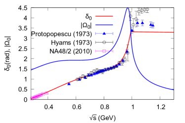
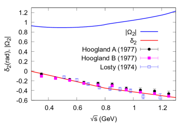
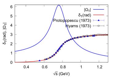
Figure 1: The S- and P-wave $\pi\pi$ scattering phase-shifts and the corresponding Omnès functions. The experimental data shown are from refs. [67, 72, 74, 75], see the discussion in the text.

In the energy range where elastic unitarity holds, the absorptive parts are therefore known in terms of the angular averages (4.5) and (4.6) supplemented by some input for the elastic $\pi\pi$ phase shifts. Measurements of the pion-pion phase-shifts have been performed in a large number of production experiments, $\pi N\to\pi\pi N,\pi\pi\Delta$ in the 1970’s, see [66] for a review. Alternative information on the phase-shifts can be obtained from $\pi\pi$ form factors in semi-leptonic or electromagnetic processes. For instance, information on the phase $\delta_{0}(s)$ at low energy can be extracted from $K_{l4}$ decays, the most precise results coming from the NA48/2 experiment [67]. The difference of the two $I=0$ and $I=2$ S-wave phases at $s=M_{K}^{2}$ can be derived from the widths of the three $K\to\pi\pi$ decay modes, up to some isospin breaking corrections. An updated evaluation of these has been performed in ref. [68], leading to the following result

$$\Delta\equiv\delta_{0}(M_{K}^{2})-\delta_{2}(M_{K}^{2})=(52.5\pm 0.8\pm 2.8)^{\circ}$$ (4.18)

which is compatible, within one sigma, with the result obtained from the production experiments also constrained with the dispersive Roy equations: $\Delta=(47.7\pm 1.5)^{\circ}$ (ref. [69]), $\Delta=(50.5\pm 1.2)^{\circ}$ (ref. [70]). Finally, data on the pion vector form factor, as measured in $e^{+}e^{-}$ scattering or $\tau$ decays can be used to obtain an alternative determination of the P-wave phase $\delta_{1}$ below 1 GeV, see for instance ref. [71]. The phases used in the present work, and the corresponding Omnès functions, are illustrated on Fig. 1. The fitting curves (shown as red lines in the figure) correspond to Roy equations solutions from ref. [71] in the region $\sqrt{s}\leq 0.8$ GeV and the three phases are assumed to be constant, equal to their asymptotic values (4.16), when $\sqrt{s}\geq 3.16$ GeV. In the intermediate energy region, in the case of $\delta_{1}$ the curve corresponds to a fit of the data in the range $[0.8,1.45]$ GeV, using a K-matrix description as in ref. [72] and a simple interpolation [73] to the asymptotic value above $1.45$ GeV. In the case of $\delta_{0}$, the data is fitted in the range $[0.8,1]$ GeV using a functional form which is also constrained by the Roy equations, see ref. [76], and interpolated to $\pi$ beyond this energy range [73]. Finally, for $\delta_{2}$ the experimental data is fitted in the range $[0.8,1.2]$ GeV with a simple polynomial function and interpolated to zero above $1.2$ GeV.

5 Omnès-Khuri-Treiman integral equations

In the approximation where the final state interactions are restricted to elastic rescattering of the pion pairs, the system of dispersion relations (3.6) seems now to be complete, with the absorptive parts given by eq. (4.17). There are, however, a couple of well-known issues that still need to be dealt with before proceeding with the numerical solution of this system. On the one side, it has been observed long ago [5, 10] that without the second contribution, given by ${\hat{M}}_{1,3}^{I;{\cal I}}(s)$, in the absorptive parts, the dispersion relations would take the form of an Omnès problem. On the other side, in the form provided by eqs. (3.6) and (4.17), the dispersion relations do in general not lead to a unique set of solutions [14]. Both issues can be dealt with, and in particular unique solutions are expected, if the dispersion relations are written instead for the functions $M_{1,3}^{I;{\cal I}}(s)/\Omega_{I}(s)$, where $\Omega_{I}(s)$ denote the Omnès factors

$$\Omega_{I}(s)={\rm exp}\left[\frac{s}{\pi}\int_{4M_{\pi}^{2}}^{+\infty}\frac{dx}{x}\,\frac{\delta_{I}(x)}{x-s}\right],$$ (5.1)

with their asymptotic behaviours for $s\to\infty$ given, according to Eq. (4.16), by

$$\Omega_{0}(s)\sim\frac{1}{s},\ \ \Omega_{1}(s)\sim\frac{1}{s},\ \ \Omega_{2}(s)\sim{\rm constant}.$$ (5.2)

This gives the set of Omnès-Khuri-Treiman integral equations

$$M_{1,3}^{I;{\cal I}}(s)=\Omega_{I}(s)\left\{P_{1,3}^{I;{\cal I}}(s)+\frac{s^{n_{1,3}^{I;{\cal I}}}}{\pi}\int_{4M_{\pi}^{2}}^{\infty}\frac{dx}{x^{n_{1,3}^{I;{\cal I}}}}\,\frac{\sin\delta_{I}(x){\hat{M}}_{1,3}^{I;{\cal I}}(x)}{|\Omega_{I}(x)|(x-s)}\right\},\quad I=0,1,2,\ {\cal I}=\frac{1}{2},\,\frac{3}{2}.$$ (5.3)

Here, $P_{1,3}^{I;{\cal I}}(s)$ are subtraction polynomials whose orders depend on the asymptotic conditions assumed for the amplitudes and on the additional constraints that were put on their behaviour at $s=0$. Before giving the explicit form of the subtraction polynomials that follow from these restrictions, we observe that the expression of the absorptive part of any function ${\hat{M}}_{1,3}^{I;{\cal I}}(s)$ in eqs. (4.5) or (4.6) involves almost all the other functions, $M_{1}^{I;{\cal I}}(s)$ or $M_{3}^{I;{\cal I}}(s)$, respectively. By forming appropriate linear combinations of the isospin functions, one may decompose the relations (4.5) or (4.6) into subsets that do not mix with the other subsets when taking the partial-wave projections. Let us therefore define

$$\left(\begin{tabular}[]{c}$M_{2}(s)$\\ $M_{1}(s)$\\ ${\tilde{M}}_{1}(s)$\\ $M_{0}(s)$\end{tabular}\right)=\left(\begin{tabular}[]{cccc}$1$&0&0&0\\[2.84544pt] 0&$\frac{1}{3}$&$\frac{2}{3}$&0\\[2.84544pt] 0&$\frac{2}{3}$&$-\frac{2}{3}~{}~{}$&0\\[2.84544pt] 0&0&0&1\end{tabular}\right)\left(\begin{tabular}[]{c}$M_{1}^{2;\frac{3}{2}}(s)$\\ $M_{1}^{1;\frac{3}{2}}(s)$\\ $M_{1}^{1;\frac{1}{2}}(s)$\\ $M_{1}^{0;\frac{1}{2}}(s)$\end{tabular}\right)$$ (5.4)

and

$$\left(\begin{tabular}[]{c}${N}_{2}(s)$\\ ${\tilde{N}}_{2}(s)$\\ ${N}_{1}(s)$\\ ${\tilde{N}}_{1}(s)$\\ ${N}_{0}(s)$\end{tabular}\right)=\left(\begin{tabular}[]{ccccc}$\frac{1}{2}$&$\!\!\frac{1}{2}$&$\!\!\!\!\!0$&$\!\!\!0$&$\!\!\!0$\\[2.84544pt] $1$&$\!\!\!-1~{}~{}$&$\!\!\!\!\!0$&$\!\!\!0$&$\!\!\!0$\\[2.84544pt] 0&$\!\!\!0$&$\!\!\!\!\!\frac{5}{6}$&$\!\!\!\frac{1}{6}$&$\!\!\!0$\\[2.84544pt] 0&$\!\!\!0$&$\!\!\!\!\!-\frac{1}{3}~{}~{}$&$\!\!\!\frac{1}{3}$&$\!\!\!0$\\[2.84544pt] 0&$\!\!\!0$&$\!\!\!\!\!0$&$\!\!\!0$&$\!\!\!1$\end{tabular}\right)\!\left(\begin{tabular}[]{c}$M_{3}^{2;\frac{3}{2}}(s)$\\ $M_{3}^{2;\frac{1}{2}}(s)$\\ $M_{3}^{1;\frac{3}{2}}(s)$\\ $M_{3}^{1;\frac{1}{2}}(s)$\\ $M_{3}^{0;\frac{3}{2}}(s)$\end{tabular}\right).$$ (5.5)

The corresponding absorptive parts are then given by

$${\hat{M}}_{2} = \langle M_{0}\rangle+\frac{1}{3}\langle M_{2}\rangle-\frac{3}{2}(s-s_{0})\langle M_{1}\rangle-\frac{1}{2}\kappa\langle zM_{1}\rangle,$$

$${\hat{M}}_{1} = \frac{1}{\kappa}\left[3\langle zM_{0}\rangle-5\langle zM_{2}\rangle+\frac{9}{2}(s-s_{0})\langle zM_{1}\rangle+\frac{3}{2}\kappa\langle z^{2}M_{1}\rangle\right],$$

$${\hat{M}}_{0} = \frac{2}{3}\langle M_{0}\rangle+\frac{20}{9}\langle M_{2}\rangle+2(s-s_{0})\langle M_{1}\rangle+\frac{2}{3}\kappa\langle zM_{1}\rangle,$$

$${\hat{\tilde{M}}}_{1} = \frac{1}{\kappa}\left[-9(s-s_{0})\langle z{\tilde{M}}_{1}\rangle-3\kappa\langle z^{2}{\tilde{M}}_{1}\rangle\right]$$

and

$${\hat{N}}_{2} = \langle{N}_{0}\rangle+\frac{1}{3}\langle{N}_{2}\rangle-\frac{3}{2}(s-s_{0})\langle{N}_{1}\rangle-\frac{1}{2}\kappa\langle z{N}_{1}\rangle,$$

$${\hat{N}}_{1} = \frac{1}{\kappa}\left[3\langle z{N}_{0}\rangle-5\langle z{N}_{2}\rangle+\frac{9}{2}(s-s_{0})\langle z{N}_{1}\rangle+\frac{3}{2}\kappa\langle z^{2}{N}_{1}\rangle\right],$$

$${\hat{N}}_{0} = \frac{2}{3}\langle{N}_{0}\rangle+\frac{20}{9}\langle{N}_{2}\rangle+2(s-s_{0})\langle{N}_{1}\rangle+\frac{2}{3}\kappa\langle z{N}_{1}\rangle,$$

$${\hat{\tilde{N}}}_{2} = -\langle{\tilde{N}}_{2}\rangle-\frac{9}{2}(s-s_{0})\langle{\tilde{N}}_{1}\rangle-\frac{3}{2}\kappa\langle z{\tilde{N}}_{2}\rangle,$$

$${\hat{\tilde{N}}}_{1} = \frac{1}{\kappa}\left[-3\langle z{\tilde{N}}_{2}\rangle+\frac{9}{2}(s-s_{0})\langle z{\tilde{N}}_{1}\rangle+\frac{3}{2}\kappa\langle z^{2}{\tilde{N}}_{1}\rangle\right].$$

For the functions related to the $\Delta I=1/2$ transitions, we observe that there are two disconnected subsets, the second one consisting of the single function ${\tilde{M}}_{1}(s)$, whose absorptive part depends on none of the other functions, while this function in turn does not appear in the absorptive parts of the other three functions $M_{0,1,2}(s)$. Likewise, the functions related to the $\Delta I=3/2$ transitions separate into two disconnected sets, consisting of the three functions $N_{0,1,2}(s)$ and the two functions ${\tilde{N}}_{1,2}(s)$. It is also of interest to notice that the numerical coefficients in front of the functions ${M}_{0,1,2}$ entering the definitions of the functions ${\hat{M}}_{0,1,2}$ are the same as those that define the functions ${\hat{N}}_{0,1,2}$ in terms of the functions $N_{0,1,2}$. In addition, the function $N_{1}(s)$ is proportional to the combination $5M_{3}^{1;\frac{3}{2}}(s)+M_{3}^{1;\frac{1}{2}}(s)$ that we had singled out at the end of Section 3 for precisely this purpose. These features will be useful in determining the number of independent solutions of the system of dispersion relations. In terms of these new functions, and taking all the contraints discussed so far into account, the dispersion relations finally take the form

$$M_{2}(s) = \Omega_{2}(s)s^{2}I_{2}(s)\hskip 145.96277ptI_{2}(s)=\frac{1}{\pi}\int_{4M_{\pi}^{2}}^{\infty}\frac{dx}{x^{2}}\,\frac{\sin\delta_{2}(x){\hat{M}}_{2}(x)}{|\Omega_{2}(x)|(x-s)},$$

$$M_{1}(s) = \Omega_{1}(s)\left\{\mu_{3}s+sI_{1}(s)\right\}\hskip 110.25443ptI_{1}(s)=\frac{1}{\pi}\int_{4M_{\pi}^{2}}^{\infty}\frac{dx}{x^{2}}\,\frac{\sin\delta_{1}(x){\hat{M}}_{1}(x)}{|\Omega_{1}(x)|(x-s)},$$

$${\tilde{M}}_{1}(s) = \Omega_{1}(s)\left\{{\tilde{\mu}}_{1}s+s{\tilde{I}}_{1}(s)\right\}\hskip 106.9822pt{\tilde{I}}_{1}(s)=\frac{1}{\pi}\int_{4M_{\pi}^{2}}^{\infty}\frac{dx}{x^{2}}\,\frac{\sin\delta_{1}(x){\hat{\tilde{M}}}_{1}(x)}{|\Omega_{1}(x)|(x-s)},$$

$$M_{0}(s) = \Omega_{0}(s)\left\{\mu_{0}+\mu_{1}s+\mu_{2}s^{2}+s^{2}I_{0}(s)\right\}\hskip 49.79231ptI_{0}(s)=\frac{1}{\pi}\int_{4M_{\pi}^{2}}^{\infty}\frac{dx}{x^{2}}\,\frac{\sin\delta_{0}(x){\hat{M}}_{0}(x)}{|\Omega_{0}(x)|(x-s)}$$ (5.8)

and

$$N_{2}(s) = \Omega_{2}(s)s^{2}J_{2}(s)\hskip 142.26378ptJ_{2}(s)=\frac{1}{\pi}\int_{4M_{\pi}^{2}}^{\infty}\frac{dx}{x^{2}}\,\frac{\sin\delta_{2}(x){\hat{N}}_{2}(x)}{|\Omega_{2}(x)|(x-s)},$$

$${\tilde{N}}_{2}(s) = \Omega_{2}(s)s^{2}{\tilde{J}}_{2}(s)\hskip 142.26378pt{\tilde{J}}_{2}(s)=\frac{1}{\pi}\int_{4M_{\pi}^{2}}^{\infty}\frac{dx}{x^{2}}\,\frac{\sin\delta_{2}(x){\hat{\tilde{N}}}_{2}(x)}{|\Omega_{2}(x)|(x-s)},$$

$$N_{1}(s) = \Omega_{1}(s)\left\{\nu_{3}s+sJ_{1}(s)\right\}\hskip 106.69783ptJ_{1}(s)=\frac{1}{\pi}\int_{4M_{\pi}^{2}}^{\infty}\frac{dx}{x}\,\frac{\sin\delta_{1}(x){\hat{N}}_{1}(x)}{|\Omega_{1}(x)|(x-s)},$$

$${\tilde{N}}_{1}(s) = \Omega_{1}(s)\left\{{\tilde{\nu}}_{0}+{\tilde{\nu}}_{1}s+s{\tilde{J}}_{1}(s)\right\}\hskip 81.09052pt{\tilde{J}}_{1}(s)=\frac{1}{\pi}\int_{4M_{\pi}^{2}}^{\infty}\frac{dx}{x}\,\frac{\sin\delta_{1}(x){\hat{\tilde{N}}}_{1}(x)}{|\Omega_{1}(x)|(x-s)},$$

$$N_{0}(s) = \Omega_{0}(s)\left\{\nu_{0}+{\nu}_{1}s+{\nu}_{2}s^{2}+s^{2}J_{0}(s)\right\}\hskip 46.94687ptJ_{0}(s)=\frac{1}{\pi}\int_{4M_{\pi}^{2}}^{\infty}\frac{dx}{x^{2}}\,\frac{\sin\delta_{0}(x){\hat{N}}_{0}(x)}{|\Omega_{0}(x)|(x-s)}.$$ (5.9)

When restricted to either one of the two subsets $M_{0,1,2}(s)$ and $N_{0,1,2}(s)$, the equations (5) and (5) or (5) and (5) are exactly the same as those found in the literature for the $\eta\to\pi\pi\pi$ amplitudes, except that the function $\kappa(s)$ and the constant $s_{0}$ are now defined in terms of the kaon mass $M_{K}$ and not of the eta-meson mass. In the case of the $\eta\to\pi\pi\pi$ transitions, the total isospin of the three pions is necessarily equal to unity (if only first-order isospin-breaking effects are retained). It is thus obvious that the two sets of functions $M_{0,1,2}(s)$ and $N_{0,1,2}(s)$ describe the kaon decays into three pions in a state of total isospin one. The functions ${\tilde{M}}_{1}$, ${\tilde{N}}_{1}$, and ${\tilde{N}}_{2}$ have no counterpart in the case of the eta meson, and reflect the transition to a state of total isospin zero in the case of ${\tilde{M}}_{1}$, or of total isospin two in the case of ${\tilde{N}}_{1}$ and ${\tilde{N}}_{2}$.

Solutions to the set of integral equations (5) and (5) are generated numerically, given as input a set of $\pi\pi$ scattering phases. The latter have been discussed at the end of section 4. The solutions are obtained through an iterative process, putting all the hatted functions ${\hat{M}}_{I}$, ${\hat{N}}_{I}$, … equal to zero as the starting point of the iteration. This numerical treatment is well documented in the literature, see for instance the references [13, 14, 19, 16, 18] for more complete discussions. Let us simply recall here that since the equations are linear, each single-variable function will take the form of a linear combination of the subtraction constants multiplied by certain coefficient functions. The latter can be obtained by successively taking one subtraction constant equal to unity while putting all the remaining ones to zero. Therefore, they do not depend on the subtraction constants anymore. Taking also into account the observations made after eq. (5), the solution of the system of integral equations (5) and (5) thus writes as

$$\left(\!\!\begin{tabular}[]{c}$M_{I}(s)$\\ $N_{I}(s)$\end{tabular}\!\!\right) = \left(\!\!\begin{tabular}[]{c}$\mu_{0}$\\ $\nu_{0}$\end{tabular}\!\!\right){\cal S}_{I}^{(0)}(s)+\left(\!\!\begin{tabular}[]{c}$\mu_{1}$\\ $\nu_{1}$\end{tabular}\!\!\right){\cal S}_{I}^{(1)}(s)+\left(\!\!\begin{tabular}[]{c}$\mu_{2}$\\ $\nu_{2}$\end{tabular}\!\!\right){\cal S}_{I}^{(2)}(s)+\left(\!\!\begin{tabular}[]{c}$\mu_{3}$\\ $\nu_{3}$\end{tabular}\!\!\right){\cal S}_{I}^{(3)}(s),\quad I=0,1,2$$ (5.20)

$${\tilde{M}}_{1}(s) = {\tilde{\mu}}_{1}{\tilde{\cal S}}_{1}(s),~{}~{}~{}~{}~{}{\tilde{N}}_{I}(s)={\tilde{\nu}}_{0}{\tilde{\cal S}}_{I}^{(0)}+{\tilde{\nu}}_{1}{\tilde{\cal S}}_{I}^{(1)},\quad I=1,2.$$

This general solution depends only on 17 independent functions, called fundamental solutions, that remain to be determined numerically, through the iterative process described above. Tables of these numerical solutions, together with the set of phase shifts used as input, are provided as ancillary files. Plots of the fundamental solutions are shown in Figs. 2.

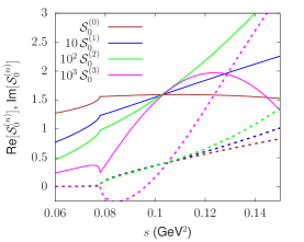
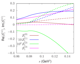
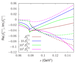
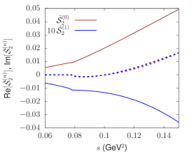
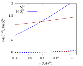
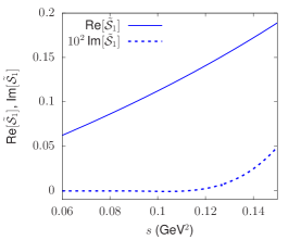
Figure 2: The upper panel displays the plots of the fundamental solutions ${\cal S}^{(n)}_{I}(s)$ associated with the single-variable functions $M_{I}(s)$ and $N_{I}(s)$. The left, central, and right windows correspond to $I=0,1,2$, respectively. The lower panel shows the plots of the fundamental solutions ${\tilde{\cal S}}_{2}^{(0)}(s)$ (in red) and ${\tilde{\cal S}}_{2}^{(1)}(s)$ (in blue), associated with the function $\tilde{N}_{2}(s)$ (left window), ${\tilde{\cal S}}_{1}^{(0)}(s)$ (in red) and ${\tilde{\cal S}}_{1}^{(1)}(s)$ (in blue), associated with the function $\tilde{N}_{1}(s)$ (central window), and ${\tilde{\cal S}}_{1}(s)$ corresponding to ${\tilde{M}}_{1}(s)$ (right window). The solid lines represent the real parts of the functions and the dashed lines the corresponding imaginary parts. The cusps originating from two-pion thresholds at $s=4M_{\pi}^{2}=0.078$ GeV² are clearly visible in most of the plots. The decay region corresponds to the interval $4M_{\pi}^{2}\leq s\leq(M_{K}-M_{\pi})^{2}=0.127\,{\rm GeV}^{2}$. Notice that the units on the vertical axes depend on the function under consideration and are expressed in powers of GeV according to Table 2.

$N$	subtraction csts.	fundamental functions
$-4$	$\mu_{2},\mu_{3},\nu_{2},\nu_{3},{\tilde{\mu}}_{1},{\tilde{\nu}}_{1}$	$-$
$-2$	$\mu_{1},\nu_{1},{\tilde{\nu}}_{0}$	${\cal S}_{1}^{(0)}$
$~{}~{}0$	$\mu_{0},\nu_{0}$	${\cal S}_{0}^{(0)},{\cal S}_{2}^{(0)},{\cal S}_{1}^{(1)},{\tilde{\cal S}}_{1}^{(0)}$
$+2$	$-$	${\cal S}_{0}^{(1)},{\cal S}_{2}^{(1)},{\cal S}_{1}^{(2)},{\cal S}_{1}^{(3)},{\tilde{\cal S}}_{1}^{(1)},{\tilde{\cal S}}_{2}^{(0)},{\tilde{\cal S}}_{1}$
$+4$	$-$	${\cal S}_{0}^{(2)},{\cal S}_{2}^{(2)},{\cal S}_{0}^{(3)},{\cal S}_{2}^{(3)},{\tilde{\cal S}}_{2}^{(1)}$

Table 2: Dimensions in GeV^N of the various quantities involved in eq. (5.20).

The corresponding expressions for the $K\to\pi\pi\pi$ decay amplitudes read

$${\cal A}^{K^{\pm}\to\pi^{\pm}\pi^{\pm}\pi^{\mp}}(s_{1},s_{2},s_{3})\!\!\! = \!\!\!-2M_{2}(s_{3})-\frac{1}{3}\left[M_{2}(s_{1})+M_{2}(s_{2})\right]-M_{0}(s_{1})-M_{0}(s_{2})+(s_{3}-s_{1})M_{1}(s_{2})+(s_{3}-s_{2})M_{1}(s_{1})$$

$$\!\!\!-\,2N_{2}(s_{3})-{\tilde{N}}_{2}(s_{3})-\frac{1}{6}\left[2N_{2}(s_{1})-3{\tilde{N}}_{2}(s_{1})\right]-N_{0}(s_{1})-\frac{1}{6}\left[2N_{2}(s_{2})-3{\tilde{N}}_{2}(s_{2})\right]-N_{0}(s_{2})$$

$$\!\!\!+\,\frac{1}{2}(s_{3}-s_{2})\left[2N_{1}(s_{1})+3{\tilde{N}}_{1}(s_{1})\right]+\frac{1}{2}(s_{3}-s_{1})\left[2N_{1}(s_{2})+3{\tilde{N}}_{1}(s_{2})\right],$$

$${\cal A}^{K^{\pm}\to\pi^{0}\pi^{0}\pi^{\pm}}(s_{1},s_{2},s_{3})\!\!\! = \!\!\!M_{0}(s_{3})-\frac{2}{3}M_{2}(s_{3})+M_{2}(s_{1})+M_{2}(s_{2})+(s_{3}-s_{1})M_{1}(s_{2})+(s_{3}-s_{2})M_{1}(s_{1})$$

$$\!\!\!+\,N_{0}(s_{3})-\frac{1}{3}\left[2N_{2}(s_{3})-3{\tilde{N}}_{2}(s_{3})\right]+\frac{1}{2}\left[2N_{2}(s_{1})-{\tilde{N}}_{2}(s_{1})\right]+\frac{1}{2}\left[2N_{2}(s_{2})-{\tilde{N}}_{2}(s_{2})\right]$$

$$\!\!\!+\,\frac{1}{2}(s_{3}-s_{2})\left[2N_{1}(s_{1})-3{\tilde{N}}_{1}(s_{1})\right]+\frac{1}{2}(s_{3}-s_{1})\left[2N_{1}(s_{2})-3{\tilde{N}}_{1}(s_{2})\right],$$

$${\cal A}^{K_{L}\to\pi^{+}\pi^{-}\pi^{0}}(s_{1},s_{2},s_{3})\!\!\! = \!\!\!-M_{0}(s_{3})+\frac{2}{3}M_{2}(s_{3})-M_{2}(s_{1})-M_{2}(s_{2})-(s_{3}-s_{1})M_{1}(s_{2})-(s_{3}-s_{2})M_{1}(s_{1})$$

$$\!\!\!+\,2N_{0}(s_{3})-\frac{4}{3}N_{2}(s_{3})+2N_{2}(s_{1})+2N_{2}(s_{2})+2(s_{3}-s_{1})N_{1}(s_{2})+2(s_{3}-s_{2})N_{1}(s_{1}),$$

$${\cal A}^{K_{S}\to\pi^{+}\pi^{-}\pi^{0}}(s_{1},s_{2},s_{3})\!\!\! = \!\!\!(s_{1}-s_{2}){\tilde{M}}_{1}(s_{3})+(s_{2}-s_{3}){\tilde{M}}_{1}(s_{1})+(s_{3}-s_{1}){\tilde{M}}_{1}(s_{2})$$

$$\!\!\!+\,{\tilde{N}}_{2}(s_{1})-{\tilde{N}}_{2}(s_{2})+(s_{3}-s_{1}){\tilde{N}}_{1}(s_{2})-(s_{3}-s_{2}){\tilde{N}}_{1}(s_{1})-2(s_{1}-s_{2}){\tilde{N}}_{1}(s_{3}),$$

$${\cal A}^{K_{L}\to\pi^{0}\pi^{0}\pi^{0}}(s_{1},s_{2},s_{3})\!\!\! = \!\!\!\left[M_{0}(s_{1})+M_{0}(s_{2})+M_{0}(s_{3})\right]+\frac{4}{3}\left[M_{2}(s_{1})+M_{2}(s_{2})+M_{2}(s_{3})\right]$$ (5.22)

$$\!\!\!-\,2\left[N_{0}(s_{1})+N_{0}(s_{2})+N_{0}(s_{3})\right]-\frac{8}{3}\left[N_{2}(s_{1})+N_{2}(s_{2})+N_{2}(s_{3})\right].$$

The $K\pi\to\pi\pi$ amplitudes listed in Table 1 can then be obtained from the above amplitudes through crossing. In particular, with the phase convention we have been using, one has ${\cal A}_{1}(s,t,u)=-{\cal A}^{K^{\pm}\to\pi^{\pm}\pi^{\pm}\pi^{\mp}}(t,u,s)$, ${\cal A}_{4}(s,t,u)=-{\cal A}^{K^{\pm}\to\pi^{0}\pi^{0}\pi^{\pm}}(t,u,s)$, $\sqrt{2}\,{\cal A}_{13}(s,t,u)$ $={\cal A}^{K_{L}\to\pi^{0}\pi^{0}\pi^{0}}(s,t,u)$ and

$$\sqrt{2}\,{\cal A}_{7}(s,t,u)={\cal A}^{K_{L}\to\pi^{+}\pi^{-}\pi^{0}}(t,u,s)+{\cal A}^{K_{S}\to\pi^{+}\pi^{-}\pi^{0}}(t,u,s).$$ (5.23)

Finally, one also needs to fix the numerical values of the eleven subtraction constants in eq. (5.20). This last issue is addressed in the next section.

6 Fixing the subtraction constants and a few applications

Since the system of Omnès-Khuri-Treiman equations does not provide information on the subtraction constants themselves, some external information is required for their determination. Moreover, the subtraction constants are in general complex numbers. We will follow a procedure that allows for a determination of all subtraction constants but one, ${\tilde{\mu}}_{1}$, based on the two following observations:

• In the region close to $s=0$, where the low-energy expansion is reliable, the imaginary parts of the single-variable functions are only generated at the two-loop level, and are thus expected to remain small near $s=0$. Neglecting these imaginary parts in the first coefficients of the Taylor expansion at $s=0$ of the single-variable functions will provide a relation between the real and imaginary parts of the subtraction constants.

• From an experimental point of view, information on the Dalitz-plot structure and partial widths of all the $K\to\pi\pi\pi$ decay modes is available.

Taken together, these two points allow us to obtain numerical values for ten out of the eleven complex subtraction constants. The remainder of this section is devoted to the implementation of this procedure and to providing the necessary details. The particular case of ${\tilde{\mu}}_{1}$, which escapes this analysis, will be briefly addressed separately. We will then provide two simple illustrations of our results, the first one regarding the description of the $K\to\pi\pi\pi$ amplitudes as complex second-order polynomials in the variables $s_{i}-s_{0}$, the second one concerning the determination of the strong phases of these amplitudes.

6.1 Relating the real and imaginary parts of the subtraction constants

For small values of $s$, the low-energy expansion is expected to provide an accurate description of the single-variable functions, in the form of an expansion in powers of $s$. This description thus amounts to retaining only the first terms of the Taylor expansions of the single-variable functions at $s=0$. In particular, the Taylor coefficients of the constant and linear terms (quadratic terms), being generated at lowest (next-to-lowest) order in the low-energy expansion, will only receive imaginary parts from higher orders, which will thus be quite small compared to their real parts. It is therefore a good approximation to assume that the imaginary parts of these lowest Taylor coefficients vanish. At this point, we need to recall that the single-variable functions are defined only modulo polynomial ambiguities, as discussed in section 3. These ambiguities will also affect the coefficients of their Taylor expansions, and one has to work in terms of Taylor invariants [16], i.e. combinations of the Taylor coefficients that remain unchanged under these polynomial shifts in the single-variable functions. Expressed in terms of the basis of functions introduced in eqs. (5.4) and (5.5), but with the same parameters as in eqs (3.4) and (3.5), these ambiguities read

$$\delta M_{2} = \frac{b_{1}}{3}s^{3}-(c_{1}+3s_{0}b_{1})s^{2}+g_{1}s+h_{1},$$

$$\delta M_{1} = b_{1}s^{2}+c_{1}s+e_{1},$$

$$\delta{\tilde{M}}_{1} = 2a_{1}s^{3}-6s_{0}a_{1}s^{2}+2d_{1}s+2f_{1},$$

$$\delta M_{0} = -\frac{4}{9}b_{1}s^{3}+\frac{4}{3}(c_{1}+3b_{1}s_{0})s^{2}-\frac{4}{3}g_{1}s+3(s-s_{0})(g_{1}-e_{1}-3c_{1}s_{0}-6b_{1}s_{0}^{2})-\frac{4}{3}h_{1},$$ (6.1)

and

$$\delta N_{2}\!\!\! = \!\!\!\frac{1}{18}(5a_{3}+c_{3})s^{3}-\frac{1}{6}(5b_{3}+d_{3}+15a_{3}s_{0}+3c_{3}s_{0})s^{2}+\frac{1}{2}(e_{3}-f_{3}+2g_{3}+3b_{3}s_{0}-3d_{3}s_{0}+6a_{3}s_{0}^{2}-6c_{3}s_{0}^{2})s+\frac{h_{3}+k_{3}}{2},$$

$$\delta{\tilde{N}}_{2}\!\!\! = \!\!\!-\frac{1}{3}(a_{3}-c_{3})s^{3}+(b_{3}-d_{3}+3a_{3}s_{0}-3c_{3}s_{0})s^{2}-(e_{3}-f_{3}+3b_{3}s_{0}-3d_{3}s_{0}+6a_{3}s_{0}^{2}-6c_{3}s_{0}^{2})s+h_{3}-k_{3},$$

$$\delta N_{1}\!\!\! = \!\!\!\frac{1}{6}(5a_{3}+c_{3})s^{2}+\frac{1}{6}(5b_{3}+d_{3})s+\frac{1}{6}(5e_{3}+f_{3}),$$

$$\delta{\tilde{N}}_{1}\!\!\! = \!\!\!-\frac{1}{3}(a_{3}-c_{3})s^{2}-\frac{1}{3}(b_{3}-d_{3})s-\frac{1}{3}(e_{3}-f_{3}),$$

$$\delta N_{0}\!\!\! = \!\!\!-\,\frac{2}{27}(5a_{3}+c_{3})s^{3}+\frac{2}{9}(5b_{3}+d_{3}+15a_{3}s_{0}+3c_{3}s_{0})s^{2}-\left(\frac{5}{3}e_{3}+\frac{4}{3}f_{3}-\frac{5}{3}g_{3}+5b_{3}s_{0}+4d_{3}s_{0}+10a_{3}s_{0}^{2}+8c_{3}s_{0}^{2}\right)\!s$$ (6.2)

$$\!\!+\,6(a_{3}+2c_{3})s_{0}^{3}+3(b_{3}+2d_{3})s_{0}^{2}+(e_{3}+2f_{3}-3g_{3})s_{0}-\frac{2}{3}(h_{3}+k_{3}).$$

This means that the Taylor coefficients up to the third (second) order for the functions $M_{2}$, ${\tilde{M}}_{1}$, $M_{0}$, $N_{2}$, ${\tilde{N}}_{2}$, $N_{0}$ ($M_{1}$, $N_{1}$, ${\tilde{N}}_{1}$) will be ambiguous. A couple of useful remarks can be made concerning these expressions:

• The parameters $a_{1}$, $d_{1}$ and $f_{1}$ occur only in $\delta{\tilde{M}}_{1}$, therefore there will be no Taylor invariants constructed with the low-order Taylor coefficients of the function ${\tilde{M}}_{1}(s)$. On the other hand, as can be seen in eq. (5), the function ${\tilde{M}}_{1}(s)$ contributes only to the decay amplitude $K_{S}\to\pi^{+}\pi^{-}\pi^{0}$, and in the combination

  $$(s_{1}-s_{2}){\tilde{M}}_{1}(s_{3})+(s_{2}-s_{3}){\tilde{M}}_{1}(s_{1})+(s_{3}-s_{1}){\tilde{M}}_{1}(s_{2}),$$

  to which the terms constant and linear in $s$ do not contribute anyway. Moreover, the cubic and quadratic terms enter $\delta{\tilde{M}}_{1}(s)$ in the combination $2a_{1}(s-s_{0})^{3}$ (up to linear and constant terms), which also does not contribute to the amplitude for $K_{S}\to\pi^{+}\pi^{-}\pi^{0}$.

• The three combinations of the parameters $a_{3}$…$f_{3}$ occurring in $\delta{\tilde{N}}_{1}$ are also present in $\delta{\tilde{N}}_{2}$, but the combination $h_{3}-k_{3}$ is only to be found in $\delta{\tilde{N}}_{2}$. Therefore, it will not be possible to construct a Taylor invariant involving ${\tilde{N}}_{2}(0)$, the lowest Taylor coefficient of ${\tilde{N}}_{2}(s)$ at $s=0$. Again, this constant term drops out of the amplitudes where ${\tilde{N}}_{2}(s)$ appears, see eq. (5).

The Taylor expansions of the single-variable functions themselves are in turn constructed from the corresponding expansions of the 17 independent fundamental solutions of eq. (5.20), and which we write in the following way

$${\cal S}_{I}^{(n)}(s)=A_{I}^{(n)}+sB_{I}^{(n)}+s^{2}C_{I}^{(n)}+s^{3}D_{I}^{(n)}+\cdots,~{}~{}~{}~{}~{}{\tilde{\cal S}}_{I}^{(n)}(s)={\tilde{A}}_{I}^{(n)}+s{\tilde{B}}_{I}^{(n)}+s^{2}{\tilde{C}}_{I}^{(n)}+s^{3}{\tilde{D}}_{I}^{(n)}+\cdots,$$ (6.3)

and

$${\tilde{\cal S}}_{1}(s)={\tilde{A}}_{1}+s{\tilde{B}}_{1}+s^{2}{\tilde{C}}_{1}+s^{3}{\tilde{D}}_{1}+\cdots.$$ (6.4)

The ambiguities in the Taylor coefficients of the single-variable functions are readily extracted from the expressions (6.1) and (6.2). Since there are $15+18$ ambiguous Taylor coefficients and $8+9$ parameters to describe the polynomial ambiguities, one expects $7+9$ Taylor invariants formed with the former. Of these, $4+6$ can be chosen such as to receive only contributions from the constant, linear and quadratic terms of the single-variable functions. They read

$$\sum_{n=0}^{3}\left(\!\!\begin{tabular}[]{c}$\mu_{n}$\\ $\nu_{n}$\end{tabular}\!\!\right)\left[A_{0}^{(n)}+s_{0}B_{0}^{(n)}+\frac{4}{3}(A_{2}^{(n)}+s_{0}B_{2}^{(n)})\right],$$ (6.7)

$$\sum_{n=0}^{3}\left(\!\!\begin{tabular}[]{c}$\mu_{n}$\\ $\nu_{n}$\end{tabular}\!\!\right)\left[3A_{1}^{(n)}+B_{0}^{(n)}-\frac{5}{3}B_{2}^{(n)}+9s_{0}(B_{1}^{(n)}+2s_{0}C_{1}^{(n)})\right],$$ (6.10)

$$\sum_{n=0}^{3}\left(\!\!\begin{tabular}[]{c}$\mu_{n}$\\ $\nu_{n}$\end{tabular}\!\!\right)\left[3C_{0}^{(n)}+4C_{2}^{(n)}\right],$$ (6.13)

$$\sum_{n=0}^{3}\left(\!\!\begin{tabular}[]{c}$\mu_{n}$\\ $\nu_{n}$\end{tabular}\!\!\right)\left[C_{2}^{(n)}+B_{1}^{(n)}+3s_{0}C_{1}^{(n)}\right],$$ (6.16)

(6.17)

$$\sum_{n=0,1}{\tilde{\nu}}_{n}[3{\tilde{A}}^{(n)}_{1}-{\tilde{B}}^{(n)}_{2}+9s_{0}({\tilde{B}}_{1}^{(n)}+2{\tilde{C}}_{1}^{(n)})],$$

$$\sum_{n=0,1}{\tilde{\nu}}_{n}[3{\tilde{B}}^{(n)}_{1}+{\tilde{C}}^{(n)}_{2}+9s_{0}{\tilde{C}}_{1}^{(n)}].$$

Requiring, as argued at the beginning of this subsection, that the imaginary parts of these ten Taylor invariants vanish leads to a linear relation between the imaginary parts of the ten subtraction constants $\mu_{n}$, $\nu_{n}$ and ${\tilde{\nu}}_{n}$ and their real parts. The numerical determination of the fundamental solutions obtained previously provides the values of the Taylor coefficients (6.3) and (6.4) involved in the relations (6.7). Note that ${\tilde{\mu}}_{1}$ does not show up in the latter, as could be anticipated from the discussion after eq. (6.2).

6.2 Determination of the real parts of the subtraction constants from data

In order to determine the real parts of the subtraction coefficients, we now turn to the experimental information that is available concerning the $K\to\pi\pi\pi$ amplitudes. In the isospin-symmetric limit, these amplitudes are smooth functions inside the decay region, since the cusps that are produced by $\pi\pi$ rescattering sit on its boundary. It takes isospin breaking and the small difference between the charged and the neutral pion masses to see some of these cusps moving inside the decay region, where they have been observed experimentally, both in the $K^{\pm}\to\pi^{0}\pi^{0}\pi^{\pm}$ and $K_{L}\to\pi^{0}\pi^{0}\pi^{0}$ modes, by the NA48/2 [43] and the KTeV [44] collaborations, respectively. In the absence of isospin breaking the measured decay distributions for the three-pion transitions of $K_{L}$ and $K^{\pm}$ (for $K_{S}$ see below) are currently described in terms of linear and quadratic slopes in the variables

$$Y\equiv\frac{s_{3}-s_{0}}{M_{\pi}^{2}},\quad X\equiv\frac{s_{2}-s_{1}}{M_{\pi}^{2}},$$ (6.18)

of the moduli squared of the amplitudes (5),

$$|{\cal A}(s_{1},s_{2}.s_{3})|^{2}=|{\cal A}(s_{0},s_{0},s_{0})|^{2}[1+gY+hY^{2}+kX^{2}].$$ (6.19)

Bose symmetry forbids a term linear in $X$, and in the case of $K_{L}\to\pi^{0}\pi^{0}\pi^{0}$ requires in addition $g=0$ and $k=h/3$. The normalization $|{\cal A}(s_{0},s_{0},s_{0})|^{2}$ can only be fixed from the corresponding $K\to\pi\pi\pi$ partial widths. The latter have also been measured, except for $K_{S}\to\pi^{+}\pi^{-}\pi^{0}$, whose partial width is reconstructed from the measurement of the interference parameter $\lambda$ with the amplitude of the $K_{L}\to\pi^{+}\pi^{-}\pi^{0}$ decay mode,

$$\lambda=\frac{\int_{Y_{min}}^{Y_{max}}dY\int_{0}^{X_{max}(Y)}dX{\cal A}^{K_{L}\to\pi^{+}\pi^{-}\pi^{0}}(X,Y){}^{*}{\cal A}^{K_{S}\to\pi^{+}\pi^{-}\pi^{0}}(X,Y)}{\int_{Y_{min}}^{Y_{max}}dY\int_{0}^{X_{max}(Y)}dX|{\cal A}^{K_{L}\to\pi^{+}\pi^{-}\pi^{0}}(X,Y)|^{2}},$$ (6.20)

where the integration runs over the whole decay region. The list of observables and their experimental values are displayed in the first two columns of Table 3. They are taken from ref. [45] and correspond, as far as the partial widths are concerned, to the values called PDG average in Table 6 of ref. [30]. For the Dalitz-plot observables, we differ from ref. [30] in two respects:

• since we account for the presence of imaginary parts in the decay amplitudes, the experimental value of Im$[\lambda]$ is included in the list of relevant observables. Both Re$[\lambda]$ and Im$[\lambda]$ have been measured with comparable precisions. We use the experimental values from refs. [77] and [78], which also provide the correlation between the real and imaginary parts of $\lambda$;

• as far as the quadratic slope $h$ of the $K_{L}\to\pi^{0}\pi^{0}\pi^{0}$ distribution is concerned (recall that in this case we have $g=0$ and $k=h/3$), the value quoted by the PDG [45] for $h$ is taken from ref. [44], and is derived from a fit to the KTeV data using the Cabibbo-Isidori rescattering model [79]. In this model, the parameter $h$ refers to only part of the full decay distribution. The parametrisation (6.19) obviously displays no cusp at the $\pi^{+}\pi^{-}$ threshold in the case of $K_{L}\to\pi^{0}\pi^{0}\pi^{0}$, but it can still be used provided one avoids the vicinity of the cusp region. The amplitudes generated through the Omnès-Khuri-Treiman equations do implement $\pi\pi$ rescattering but isospin-breaking corrections would need to be introduced before one can properly describe the cusp region, which is not the case in the present analysis (this was done in ref. [16] in the case of the $\eta\to 3\pi$ amplitudes). In order to circumvent this issue, we will instead use an earlier determination of the quadratic slope $h$ by the NA48 experiment [80],

  $$h=-6.1(1.0)\cdot 10^{-3}.$$ (6.21)

observables	expal values	fit values	$\chi^{2}$	$\alpha$-fit values	$\chi^{2}(\alpha$-fit)
$\Gamma[K_{L}\to\pi^{0}\pi^{0}\pi^{0}]$	$2.5417(352)$	2.5532	0.1	2.6113	3.9
$\Gamma[K_{L}\to\pi^{+}\pi^{-}\pi^{0}]$	$1.6200(102)$	1.6185	0.02	1.6105	0.9
$\Gamma[K^{+}\to\pi^{0}\pi^{0}\pi^{+}]$	$0.9438(150)$	0.8984	9.2	0.9133	4.1
$\Gamma[K^{+}\to\pi^{+}\pi^{+}\pi^{-}]$	$2.9590(218)$	2.9865	1.7	2.9779	0.8
$\Gamma[K_{S}\to\pi^{+}\pi^{-}\pi^{0}]$	$0.0026(7)$	0.0031	$-$	0.0031	$-$
$h[[K_{L}\to\pi^{0}\pi^{0}\pi^{0}]$	$-0.0061(10)$	$-0.00644$	0.1	$-0.00645$	0.1
$g[K_{L}\to\pi^{+}\pi^{-}\pi^{0}]$	$0.678(8)$	0.675	0.1	0.677	0.02
$h[K_{L}\to\pi^{+}\pi^{-}\pi^{0}]$	$0.076(6)$	0.082	0.9	0.082	0.9
$k[K_{L}\to\pi^{+}\pi^{-}\pi^{0}]$	$0.0099(15)$	0.011	0.3	0.011	0.5
$g[K^{+}\to\pi^{0}\pi^{0}\pi^{+}]$	$0.626(7)$	0.625	0.04	0.624	0.1
$h[K^{+}\to\pi^{0}\pi^{0}\pi^{+}]$	$0.052(8)$	0.058	0.6	0.063	1.9
$k[K^{+}\to\pi^{0}\pi^{0}\pi^{+}]$	$0.0054(35)$	0.011	2.7	0.012	3.5
$g[K^{+}\to\pi^{+}\pi^{+}\pi^{-}]$	$-0.21134(17)$	$-0.21134$	0	$-0.21134$	0
$h[K^{+}\to\pi^{+}\pi^{+}\pi^{-}]$	$0.0185(4)$	0.0185	0	0.0185	0
$k[K^{+}\to\pi^{+}\pi^{+}\pi^{-}]$	$-0.00463(14)$	$-0.00464$	0	$-0.00464$	0
Re$[\lambda]$	$0.0334(52)$	0.0360	0.4	0.0356	0.2
Im$[\lambda]$	$-0.0108(48)~{}\,~{}$	$-0.0092~{}\,~{}$	0.11	$-0.0091$	0.13

Table 3: The two first columns show the experimental observables and their input values used for the fits. The third and fourth columns give the results from the fits described in subsection 6.2, and the two last columns for the $\alpha$-fit described in subsection 6.3. The widths are expressed in units of $10^{-18}$ GeV. The width $\Gamma[K_{S}\to\pi^{+}\pi^{-}\pi^{0}]$ is not an independent quantity, being reconstructed from $\Gamma[K_{L}\to\pi^{+}\pi^{-}\pi^{0}]$ and $\lambda$. It is thus not an input for the fits, and is only given for completeness.

The list of experimental observables and the values we use are collected in the two first columns of Table 3. In order to proceed with the determination of the real parts of the subtraction constants, we take the modulus squared of the various amplitudes generated by our solutions (5.20), express the imaginary parts of the ten subtraction constants $\mu_{n}$, $\nu_{n}$ and ${\tilde{\nu}}_{n}$, as described in the preceding subsection, in terms of their real parts and fit the latter, in the decay regions, to the experimental descriptions (6.19) using the values given in Table 3. For this fit, ${\tilde{\mu}}_{1}$ is set to zero. The outcome of this procedure as far as the subtraction constants are concerned is displayed in Table 4. The third column in Table 3 gives the values of the observables that result from this fit and the fourth column provides the contribution of each observable to the total $\chi^{2}$ whose value is $\chi^{2}_{\rm tot}=16.1$. Given that there are six degrees of freedom, the quality of the fit as measured by the value of $\chi^{2}_{\rm tot}$ is certainly not optimal. As discussed in detail in ref. [30] this can most likely be ascribed to tensions among some of the experimental partial widths. Notwithstanding this issue with the high value of the total $\chi^{2}$, and given the 16 independent experimental data listed in Table 3, one might wonder why not also include the complex subtraction constant ${\tilde{\mu}}_{1}$ into the set of parameters to be fitted, since this would still leave us with four real degrees of freedom. The reason why this does actually not work can be understood upon looking more closely at the expression for the observable $\lambda$, which turns out, according to the eqs. (5.20) and (5), to represent the only observable sensitive to ${\tilde{\mu}}_{1}$. We defer the discussion of this issue to the subsection 6.4 below.

$n$	$\mu_{n}$	$\nu_{n}$	${\tilde{\nu}}_{n}$	${\tilde{\mu}}_{n}$
$0$	$~{}~{}~{}~{}~{}~{}\,\,~{}+3.8(4)-i0.570(2)$	$\qquad\qquad\ \,\quad-4.7(3)-i2.37(10)\cdot 10^{-2}$	$\,-2.04(1.2)+i4.8(5)\cdot 10^{-4}$	$-$
$1$	$\,~{}-676.1(4.0)+i7.27(2)$	$~{}\,+26.7(2.8)+i0.30(1)$	$+433.2(12.2)-i6.0(1.3)\cdot 10^{-4}$	n.d.
$2$	$~{}\,+559.7(18.5)-i16.80(5)$	$~{}\!-46.0(14.2)-i0.74(3)$	$-~{}\,~{}$	$-$
$3$	$-1072.6(13.6)+i7.57(2)$	$+123.9(12.6)-i0.28(1)$	$-~{}\,~{}$	$-$

Table 4: Values of the real and imaginary parts of the subtraction constants. $\mu_{0}$ and $\nu_{0}$ are dimensionless numbers, $\mu_{1},\nu_{1},{\tilde{\nu}}_{0}$ are expressed in units of GeV^-2, and the remaining subtraction constants in units of GeV^-4.

6.3 Description of the decay amplitudes as complex polynomials

As already mentioned, in the absence of isospin violation the decay amplitudes are smooth functions over the whole decay region. It is thus possible to describe them in terms of polynomials in the variables $s_{i}-s_{0}$, equivalently in the variables $X$ and $Y$ defined in eq. (6.18), corresponding to their Taylor expansions around the centre of the decay region $s_{1}=s_{2}=s_{3}=s_{0}$. From a phenomenological point of view, the decay amplitudes are well described by such polynomials truncated at second order, at least away from the narrow region of the cusp in the two cases mentioned at the beginning of the preceding subsection. In order to construct such a description we are thus led to consider the Taylor expansions of the single-variable functions at $s=s_{0}$. As before, the first task consists in dealing with the ambiguities the latter are beset with. The construction of the appropriate Taylor invariants proceeds as previously, but starting now from the Taylor expansions of the fundamental functions at $s=s_{0}$. We denote the corresponding Taylor coefficients with lower-case latin letters, i.e. in equations (6.3) and (6.4) we replace $s$ by $s-s_{0}$ and at the same time $A_{I}^{(n)}$ by $a_{I}^{(n)}$, and so on. The values of these coefficients are again provided by our numerical determination of the fundamental functions in eq. (5.20). For our purposes, the relevant Taylor invariants we can construct read

$$\sum_{n=0}^{3}\left(\!\!\begin{tabular}[]{c}$\mu_{n}$\\ $\nu_{n}$\end{tabular}\!\!\right)\left[-a_{0}^{(n)}-\frac{4}{3}a_{2}^{(n)}\right]\equiv\left(\!\!\!\begin{tabular}[]{c}${\bar{\alpha}}_{1}$\\[4.26773pt] $-{\bar{\alpha}}_{3}/2$\end{tabular}\!\!\right),$$ (6.26)

$$\sum_{n=0}^{3}\left(\!\!\begin{tabular}[]{c}$\mu_{n}$\\ $\nu_{n}$\end{tabular}\!\!\right)\left[3a_{1}^{(n)}+b_{0}^{(n)}-\frac{5}{3}b_{2}^{(n)}\right]M_{\pi}^{2}\equiv\left(\!\!\!\begin{tabular}[]{c}${\bar{\beta}}_{1}$\\[4.26773pt] $-{\bar{\beta}}_{3}/2$\end{tabular}\!\!\right),$$ (6.31)

$$\sum_{n=0}^{3}\left(\!\!\begin{tabular}[]{c}$\mu_{n}$\\ $\nu_{n}$\end{tabular}\!\!\right)\left[-c_{0}^{(n)}-\frac{4}{3}c_{2}^{(n)}\right]\frac{M_{\pi}^{4}}{2}\equiv\left(\!\!\!\begin{tabular}[]{c}${\bar{\zeta}}_{1}$\\[4.26773pt] ${\bar{\zeta}}_{3}$\end{tabular}\!\!\right),$$ (6.36)

$$\sum_{n=0}^{3}\left(\!\!\begin{tabular}[]{c}$\mu_{n}$\\ $\nu_{n}$\end{tabular}\!\!\right)\left[-c_{0}^{(n)}+\frac{5}{3}c_{2}^{(n)}+3b_{1}^{(n)}\right]\frac{M_{\pi}^{4}}{2}\equiv\left(\!\!\!\begin{tabular}[]{c}${\bar{\xi}}_{1}$\\[4.26773pt] ${\bar{\xi}}_{3}$\end{tabular}\!\!\right),$$ (6.41)

(6.42)

$$\sum_{n=0,1}{\tilde{\nu}}_{n}[3{\tilde{a}}^{(n)}_{1}-{\tilde{b}}^{(n)}_{2}]\frac{\sqrt{3}}{2}M_{\pi}^{2}\equiv{\bar{\gamma}}_{3},$$

$$\sum_{n=0,1}{\tilde{\nu}}_{n}[-3{\tilde{b}}^{(n)}_{1}-{\tilde{c}}^{(n)}_{2}]\frac{3}{4}M_{\pi}^{4}\equiv{\bar{\xi}}_{3}^{\prime}.$$

Let us observe in passing that again ${\tilde{\mu}}_{1}$ is not involved in these Taylor invariants.

The next step consists in expressing the physical amplitudes as polynomials in the variables $s_{i}-s_{0}$ truncated at second order, with coefficients given by the Taylor invariants. This calculation is straightforward, starting from eq. (5), then inserting the Taylor expansions at $s=s_{0}$ of the single-particle functions (5.20), and finally checking that the various Taylor coefficients indeed combine to yield the Taylor invariants of eq. (6.26). The result of these manipulations reads

$${\cal A}^{K_{L}\to\pi^{0}\pi^{0}\pi^{0}}(s_{1},s_{2},s_{3}) = -3({\bar{\alpha}}_{1}+{\bar{\alpha}}_{3})-3({\bar{\zeta}}_{1}-2{\bar{\zeta}}_{3})\!\left(Y^{2}+\frac{X^{2}}{3}\right),$$

$${\cal A}^{K_{L}\to\pi^{+}\pi^{-}\pi^{0}}(s_{1},s_{2},s_{3}) = {\bar{\alpha}}_{1}+{\bar{\alpha}}_{3}-({\bar{\beta}}_{1}+{\bar{\beta}}_{3})Y+({\bar{\zeta}}_{1}-2{\bar{\zeta}}_{3})\!\left(Y^{2}+\frac{X^{2}}{3}\right)\!+({\bar{\xi}}_{1}-2{\bar{\xi}}_{3})\!\left(Y^{2}-\frac{X^{2}}{3}\right)\!,$$

$${\cal A}^{K_{S}\to\pi^{+}\pi^{-}\pi^{0}}(s_{1},s_{2},s_{3}) = \frac{2}{3}\sqrt{3}{\bar{\gamma}}_{3}X-\frac{4}{3}{\bar{\xi}}_{3}\!\!{}^{\prime}\,XY,$$ (6.43)

$${\cal A}^{K^{+}\to\pi^{+}\pi^{+}\pi^{-}}(s_{1},s_{2},s_{3}) = 2{\bar{\alpha}}_{1}-{\bar{\alpha}}_{3}+({\bar{\beta}}_{1}-\frac{{\bar{\beta}}_{3}}{2}+\sqrt{3}{\bar{\gamma}}_{3})Y+2({\bar{\zeta}}_{1}+{\bar{\zeta}}_{3})\!\left(\!Y^{2}+\frac{X^{2}}{3}\right)\!-({\bar{\xi}}_{1}+{\bar{\xi}}_{3}-{\bar{\xi}}_{3}^{\prime})\!\left(\!Y^{2}-\frac{X^{2}}{3}\right)\!,$$

$${\cal A}^{K^{+}\to\pi^{0}\pi^{0}\pi^{+}}(s_{1},s_{2},s_{3}) = -({\bar{\alpha}}_{1}-\frac{{\bar{\alpha}}_{3}}{2})+({\bar{\beta}}_{1}-\frac{{\bar{\beta}}_{3}}{2}-\sqrt{3}{\bar{\gamma}}_{3})Y-({\bar{\zeta}}_{1}+{\bar{\zeta}}_{3})\!\left(\!Y^{2}+\frac{X^{2}}{3}\right)\!-({\bar{\xi}}_{1}+{\bar{\xi}}_{3}+{\bar{\xi}}_{3}^{\prime})\!\left(\!Y^{2}-\frac{X^{2}}{3}\right)\!.$$

These expressions reproduce the well known Dalitz expansions of the $K\to 3\pi$ amplitudes, implementing the constraints coming from isospin conservation [61, 62, 63, 64, 81] (we follow here the notation of [81, 27]). The expansion parameters which appear in eq. (6.3) are complex numbers (even when CP is conserved). Several approximations to their imaginary parts have been considered in the literature, for instance one-loop results [65] obtained in the low-energy expansion. But most of the time these imaginary parts have simply been discarded in fits to the experimental data relying on the expansions (6.3) [29, 27, 28, 30]. Our solutions of the Omnès-Khuri-Treiman equations instead allow one to use the expressions (6.3) together with realistic estimates of the imaginary parts. These are simply obtained from eqs. (6.26). Indeed, the linear relations which we have obtained between the real and imaginary parts of the subtraction parameters $\mu_{n}$, $\nu_{n}$, $\tilde{\nu}_{n}$ (via a matching to the low-energy expansion around $s=0$) translate, via eqs. (6.26), into a set of linear relations expressing the imaginary parts of the parameters $\bar{\alpha}_{i}$, $\bar{\beta}_{i}$, $\bar{\zeta}_{i}$, $\bar{\xi}_{i}$, $\bar{\gamma}_{3}$, $\bar{\xi}^{\prime}_{3}$ in terms of their real parts. We can then determine the latter by performing a fit to the 16 observables listed in Table 3 starting directly from the expressions (6.3) of the amplitudes, in a similar manner as done for the fit carried out in the case where the amplitude coefficients are assumed to be strictly real, as described for instance in ref [30].

The outcome of this fit (called ‘$\alpha$-fit’ to differentiate it from the fit described in subsection 6.2) is shown in Table 5. For the sake of comparison, we also show the values of the real amplitude parameters displayed in Table 5 of ref. [30] together with their imaginary parts obtained from a one-loop calculation [65, 28]. One observes that the imaginary parts of the subtraction constants are generically much smaller (in absolute values) than their real parts, but that there are substantial differences between their one-loop values and the values generated by the solutions of the Omnès-Khuri-Treiman equations, showing the effect of the resummation of final-state interactions at work in the dispersive approach. As a side remark, let us mention that determinations of $\bar{\alpha}_{1}$ and $\bar{\beta}_{1}$, based on an approximate solution of the Khuri-Treiman equations (cf. footnote 6), were also obtained by the authors of ref. [32]. The value they give for $\bar{\alpha}_{1}$ is close to the one shown in the central column of Table 5, whereas their imaginary part for $\bar{\beta}_{1}$ remains closer to the one-loop value.

The penultimate column of Table 3 shows the values obtained for the various observables from the $\alpha$-fit. They are close to the values obtained from the direct fit described in subsection 6.2, with a comparable value of the total $\chi^{2}$ value, $\chi^{2}_{\rm tot}=17.6$ (for the same number of degrees of freedom), but the contributions from the individual observables to the total $\chi^{2}$ value are somewhat different. Likewise, evaluating the complex amplitude parameters ${\bar{\alpha}}_{1,3},{\bar{\beta}}_{1,3},{\bar{\gamma}}_{3},{\bar{\zeta}}_{1,3},{\bar{\xi}}_{1,3},{\bar{\xi}}_{3}^{\prime}$ directly from their definitions (6.26) and from the fitted values of the subtraction constants $\mu_{n}$, $\nu_{n}$, ${\tilde{\nu}}_{n}$ given in Table 4 would lead to values close to the ones obtained from the $\alpha$-fit.

$\bar{\alpha}_{1}$	$91.02(22)+i18.47(4)$	$92.87(23)+i12.07(3)$
$\bar{\beta}_{1}$	$-23.73(16)-i16.32(4)$	$-26.50(16)-i12.39(3)$
$\bar{\zeta}_{1}$	$-0.33(2)+i0.27(1)$	$-0.11(2)+i0.367(4)$
$\bar{\xi}_{1}$	$-1.42(12)-i0.50(1)$	$-1.35(12)-i0.191(1)$
$\bar{\alpha}_{3}$	$-6.88(27)-i1.40(5)$	$-7.13(27)-i0.93(4)$
$\bar{\beta}_{3}$	$-2.79(24)+i0.92(4)$	$-2.53(24)+i0.74(3)$
$\bar{\zeta}_{3}$	$0.014(15)-i0.06(1)$	$-0.05(2)-i0.041(3)$
$\bar{\xi}_{3}$	$0.11(7)-i0.049(4)$	$0.03(7)-i0.018(1)$
$\bar{\gamma}_{3}$	$2.88(9)-i0.102(3)$	$2.80(9)-i0.132(4)$
$\bar{\xi}^{\prime}_{3}$	$0.59(16)-i0.088(4)$	$-0.30(16)-i0.096(3)$

Table 5: The values, in units of $10^{-8}$, of the amplitudes parameters of eq. (6.3) as obtained from the $\alpha$-fit (see main text). For comparison the last column shows the values obtained in ref. [30] from a fit to the experimental data shown in Table 3 assuming the amplitude coefficients to be real, and to which the imaginary parts computed in the one-loop approximation [65, 28] have been added afterwards.

6.4 The case of ${\tilde{\mu}}_{1}$

The sole subtraction constant that remains undetermined so far is ${\tilde{\mu}}_{1}$. It appears only in the single-variable function ${\tilde{M}}_{1}(s)$, for which it provides the normalization. This function by itself accounts for the whole $\Delta I=1/2$ contribution to the $K_{S}\to\pi^{+}\pi^{-}\pi^{0}$ amplitude (if higher partial waves are neglected), but this contribution starts only at the level of cubic terms in the expansion of the amplitudes around the point $s_{i}=s_{0}$: $K_{S}\to\pi^{+}\pi^{-}\pi^{0}$ is the only decay mode whose amplitude, up to quadratic order in $X$ and $Y$, receives contributions from the $\Delta I=3/2$ transition alone. While cubic terms are suppressed in the low-energy expansion, contributions with $\Delta I=3/2$ are expected to be suppressed with respect to the ones with $\Delta I=1/2$. It seems thus reasonable to assume that the $\Delta I=1/2$ cubic term could contribute to the decay rate on par with the $\Delta I=3/2$ linear and quadratic terms. With this term added, the amplitude reads (the Taylor coefficient ${\tilde{c}}_{1}$ is a Taylor invariant, of dimension GeV^-2)

$${\cal A}^{K_{S}\to\pi^{+}\pi^{-}\pi^{0}}(s_{1},s_{2},s_{3})=\frac{2}{3}\sqrt{3}{\bar{\gamma}}_{3}X-\frac{4}{3}{\bar{\xi}}_{3}\!\!{}^{\prime}\,XY+\frac{1}{4}{\tilde{\mu}}_{1}{\tilde{c}}_{1}M_{\pi}^{6}X(X^{2}-9Y^{2})+\cdots.$$ (6.44)

The ellipsis indicates cubic terms from the $\Delta I=3/2$ transition Hamiltonian, which should be suppressed as compared to the term proportional to ${\tilde{\mu}}_{1}$ that has been retained. The whole available experimental information on the $K_{S}\to\pi^{+}\pi^{-}\pi^{0}$ decay mode is contained in the overlap parameter $\lambda$, which also plays a role in the determination of the two subtraction constants ${\tilde{\nu}}_{0}$ and ${\tilde{\nu}}_{1}$. Keeping also the third term in (6.44), we obtain ($\lambda$ is without dimension and the numerical coefficients are expressed in appropriate powers of GeV according to Table 2)

$$10^{4}\lambda=\tilde{\nu}_{0}(6.64-i1.66)+\tilde{\nu}_{1}(0.86-i0.22)+\tilde{\mu}_{1}(-0.84-i0.22)\cdot 10^{-3}\ .$$ (6.45)

We see that the contribution proportional to $\tilde{\mu}_{1}$ is extremely suppressed. This suppression can actually be traced back to the presence of zeros in the integrand that defines $\lambda$ in eq. (6.20). This is the reason why the fit in subsection 6.2 remains, for all practical purposes, silent about $\tilde{\mu}_{1}$. In order for the contribution proportional to $\tilde{\mu}_{1}$ to be comparable with the experimental error on $\lambda$ we would need to have $\tilde{\mu}_{1}\sim 200\tilde{\nu}_{1}$ (i.e. ${\tilde{\mu}}_{1}\sim 8\cdot 10^{4}$ GeV^-4). Assuming a usual size for the $\Delta{I}=1/2$ enhancement, we would rather expect $\tilde{\mu}_{1}$ to be larger in magnitude than $\tilde{\nu}_{1}$ by a factor $10-20$. An increase in precision by a factor of ten, at least, in $\lambda$ would then be necessary in order for this observable to become eventually sensitive to the value of $\tilde{\mu}_{1}$.

6.5 Strong phases in the $K\to\pi\pi\pi$ decay amplitudes

Finally, let us close this section by recalling that the knowledge of rescattering phases generated by the strong-interaction dynamics is an important input in order to predict the size of direct violations of CP invariance in $K\to\pi\pi\pi$ decays, which are expected to be quite small [82, 83, 84, 65]. In these studies, the input for the strong phases was limited to values generated at one loop in the low-energy expansion. Our solutions of the Omnès-Khuri-Treiman equations provide a more precise determination of the strong phases of the $K\to\pi\pi\pi$ amplitudes covering the whole Dalitz plot, which could be useful for estimating the size of local CP-violation effects. We do not wish to enter a full discussion of this interesting topic here, but simply illustrate, in fig. 3, our results for the local phases generated by the elastic $\pi\pi$ rescattering in the case of the two charged kaon decay amplitudes for $K^{+}\to\pi^{+}\pi^{+}\pi^{-}$ and $K^{+}\to\pi^{0}\pi^{0}\pi^{+}$.

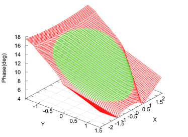
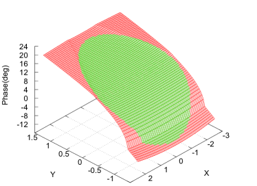
Figure 3: Strong phases (in degrees) of the $K^{+}\to\pi^{+}\pi^{+}\pi^{-}$ amplitude (left) and the $K^{+}\to\pi^{0}\pi^{0}\pi^{+}$ amplitude (right) derived from the solutions of the Omnès-Khuri-Treiman equations. The areas in green correspond to the physical decay regions.

7 Summary and conclusions

In the present work, we have implemented elastic pion-pion final-state rescattering for the amplitudes $K\pi\to\pi\pi$ within a dispersive framework of the Omnès-Khuri-Treiman-Sawyer-Wali type under the assumptions that invariance under both CP and isospin symmetry is preserved. Starting from the isospin decomposition à la Wigner-Eckart of the various amplitudes, we have identified, upon imposing the additional restrictions provided by crossing, a set of four invariant amplitudes that allows us to describe all the thirteen initial scattering amplitudes. Assuming furthermore that the imaginary parts of the partial waves higher than the P wave can be neglected, we have provided a decomposition of the invariant amplitudes in terms of a set of nine single-variable functions, see eq. (5).

The single-variable functions are analytic in the complex plane except for a right-hand cut starting at $s=4M_{\pi}^{2}$ and whose discontinuity is given by unitarity, here restricted to two-pion states. As a consequence of crossing, this ensures that the $K\pi\to\pi\pi$ amplitudes have the correct analyticity properties in the region of the Mandelstam plane below the inelastic thresholds. The single-variable functions thus obey a set of subtracted dispersion relations where the only input are the elastic $\pi\pi$ phase shifts for the S and P waves, which are well known. Using these phase shifts, we have solved these dispersion relations numerically, and obtained the solutions in terms of linear combinations of a set of fundamental functions modulated by the subtraction constants. The latter have been determined, apart from one, by matching the amplitudes constructed this way with available experimental data on the $K\to\pi\pi\pi$ decay modes, assuming that the imaginary parts of the lowest Taylor invariants of the single-variable functions vanish at the origin. The 17 independent fundamental functions, which do not depend on the subtraction constants, have been collected, in numerical form, in a series of ancillary files.

We have discussed a few applications of our results to the phenomenology of $K\to\pi\pi\pi$ decays. We have reconsidered the description of the decay amplitudes as second-order polynomials in the Dalitz-plot variables from the point of view of the dispersive approach and have shown that the corresponding amplitude coefficients, usually assumed to be real, have generically larger imaginary parts than those generated at the one-loop level. We have also determined the strong phases of the decay amplitudes of the charged kaon locally in the Dalitz plot, which can be useful for the study of possible direct violations of CP in the $K\to\pi\pi\pi$ decays.

Other approaches to determine the values of the subtraction constants could be considered [16]. For instance one could make use of the behaviour of the single-variable functions in the vicinity of the cusp at $s=4M_{\pi}^{2}$, where a non-relativistic description in terms of a power expansion with respect to the variable $q=\sqrt{s-4M_{\pi}^{2}}$ can be used. This can then be compared to the expressions obtained within an effective-theory framework in refs. [85, 86, 87]. So far, only the amplitudes for the charged kaon and the long-lived neutral kaon have been worked out within this framework, but a similar treatment of the amplitude for the decay mode $K_{S}\to\pi^{+}\pi^{-}\pi^{0}$ is missing. Therefore, a determination of all the subtraction constants (and in particular of ${\tilde{\mu}}_{1}$) is probably not possible by following this approach at the moment. In any case, the single-variable functions corresponding to alternative determinations of the subtraction constants can easily be reconstructed from the expressions given in eq. (5.20) and the fundamental functions tabulated in the ancillary files.

The results obtained in this work fill a gap in the recent literature to the extent that a full dispersive treatment of final-state interactions, albeit restricted to the elastic regime and to the absence of isospin-breaking effects, for all $K\to\pi\pi\pi$ amplitudes was not available before our work. The main objective of this study, however, is to prepare the field for applications to a class of radiative kaon-decay modes, for which more precise experimental results are expected in the future. This issue is left for forthcoming work.

Appendix A Restrictions on the isospin amplitudes from the crossing properties

In this appendix, we show how the crossing properties (2.11) of the nine isospin amplitudes in eqs. (2.7) and (2.8) lead to the general representations (2.16) and (2.17) in terms of only four independent functions. In the next appendix we provide an alternative derivation using the so-called spurion formalism.

The situation in the case of amplitudes for $K\pi\to\pi\pi$ scattering is slightly more complicated, from an algebraic point of view, than in the case of elastic pion-pion scattering. This is mainly due to the increased number of isospin amplitudes, although the amplitudes ${\vec{\cal M}}_{1}(s,t,u)$ and ${\vec{\cal M}}_{3}(s,t,u)$ can be discussed separately, which is what we will do.

Starting with the $\Delta I=1/2$ amplitudes ${\vec{\cal M}}_{1}(s,t,u)$ we define the function

$${\cal M}_{1}(s|t,u)=-{\cal A}_{4}(s,t,u)=-\frac{1}{3}{\cal M}_{1}^{2;\frac{3}{2}}(s,t,u)+\frac{1}{3}{\cal M}_{1}^{0;\frac{1}{2}}(s,t,u),$$ (A.1)

where it is understood that in this paragraph ${\cal A}_{i}(s,t,u)$ refers only to the $\Delta I=\frac{1}{2}$ component of the corresponding amplitude, related to the isospin amplitudes through the matrix ${\mathbf{R}}_{1}$ in eq. (2.9). Since ${\cal A}_{4}(s,t,u)$ corresponds to an amplitude with two neutral pions in the final state, Bose symmetry requires

$${\cal M}_{1}(s|t,u)={\cal M}_{1}(s|u,t)$$ (A.2)

while crossing gives

$${\cal A}_{5}(s,t,u)=-{\cal A}_{4}(u,t,s)={\cal M}_{1}(u|s,t),$$ (A.3)

In addition, from the relations

$${\cal M}_{1}^{2;\frac{3}{2}}(s,t,u)={\cal A}_{1}(s,t,u)={\cal A}_{2}(s,t,u)+{\cal A}_{4}(s,t,u)+{\cal A}_{5}(s,t,u)$$ (A.4)

and ${\cal A}_{2}(s,t,u)={\cal A}_{1}(u,t,s)$, one deduces that

$${\cal A}_{2}(s,t,u)-{\cal A}_{2}(u,t,s)={\cal M}_{1}(s|u,t)-{\cal M}_{1}(u|s,t)$$ (A.5)

Next, from the ${\mathbf{R}}_{1}$ part of eq. (2.9) we establish the relations

$$\frac{2}{3}{\cal M}_{1}^{2;\frac{3}{2}}(s,t,u)+\frac{1}{3}{\cal M}_{1}^{0;\frac{1}{2}}(s,t,u)=\sqrt{2}{\cal A}_{13}(s,t,u)={\cal A}_{2}(s,t,u)+{\cal A}_{5}(s,t,u)={\cal A}_{1}(s,t,u)-{\cal A}_{4}(s,t,u).$$ (A.6)

But ${\cal A}_{13}(s,t,u)$ has to be fully symmetric under permutations of the variables $s$, $t$, $u$. Therefore one obtains

$${\cal A}_{2}(s,t,u)={\cal M}_{1}(s|u,t)+{\cal M}_{1}(t|s,u)+{\widetilde{\cal M}}(s,t,u)$$ (A.7)

where ${\widetilde{\cal M}}(s,t,u)$ has the same symmetry properties as ${\cal A}_{13}(s,t,u)$. This expression of ${\cal A}_{2}(s,t,u)$ also satisfies the previous condition (A.5). Thus, from the analysis involving so far only the amplitudes with a charged kaon and the fully symmetric amplitude ${\cal A}_{13}(s,t,u)$, we have obtained

$$\sqrt{2}{\cal A}_{13}(s,t,u)={\cal M}_{1}(s|u,t)+{\cal M}_{1}(t|s,u)+{\cal M}_{1}(u|s,t)+{\widetilde{\cal M}}(s,t,u)$$ (A.8)

and

$${\cal M}_{1}^{2;\frac{3}{2}}(s,t,u) = {\cal M}_{1}(t|s,u)+{\cal M}_{1}(u|s,t)+{\widetilde{\cal M}}(s,t,u)$$

$${\cal M}_{1}^{0;\frac{1}{2}}(s,t,u) = {\cal M}_{1}(t|s,u)+{\cal M}_{1}(u|s,t)+3{\cal M}_{1}(s|u,t)+{\widetilde{\cal M}}(s,t,u)$$

$$\frac{1}{3}{\cal M}_{1}^{1;\frac{3}{2}}(s,t,u)+\frac{2}{3}{\cal M}_{1}^{1;\frac{1}{2}}(s,t,u) = {\cal M}_{1}(t|s,u)-{\cal M}_{1}(u|s,t)+{\widetilde{\cal M}}(s,t,u).$$ (A.9)

The left-hand side of the last relation, which follows from the expression of ${\cal A}_{2}(s,t,u)$ in terms of the isospin amplitudes ${\vec{\cal M}}_{1}(s,t,u)$ and the two preceding relations, involves a combination of two amplitudes where the final pions are in an isospin state $I=1$. Bose symmetry then requires this combination, and hence the combination occuring on the right-hand side of this relation, to be antisymmetric under exchange of $t$ and $u$. This immediately implies ${\widetilde{\cal M}}(s,t,u)=0$. Looking now at the amplitudes involving the neutral kaon, one finds the relation

$$\frac{1}{\sqrt{2}}{\cal M}_{1}^{2;\frac{3}{2}}(s,t,u)={\cal A}_{13}(s,t,u)+{\cal A}_{7}(s,t,u)-\frac{1}{2}{\cal A}_{9}(s,t,u)+\frac{1}{2}{\cal A}_{11}(s,t,u)$$ (A.10)

This means

$${\cal A}_{7}(s,t,u)+\frac{1}{2}{\cal A}_{7}(u,t,s)-\frac{1}{2}{\cal A}_{7}(u,s,t)=-\frac{1}{\sqrt{2}}{\cal M}_{1}(s|t,u),$$ (A.11)

from which one deduces that

$${\cal A}_{7}(s,t,u)=-\frac{1}{\sqrt{2}}[{\cal M}_{1}(s|t,u)+{\cal N}_{1}(s,t,u)]$$ (A.12)

with $2{\cal N}_{1}(s,t,u)+{\cal N}_{1}(u,t,s)-{\cal N}_{1}(u,s,t)=0$, which in turn implies that ${\cal N}_{1}(s,t,u)=-{\cal N}_{1}(t,s,u)$. Another relation,

$$\frac{1}{\sqrt{2}}{\cal M}_{1}^{1;\frac{3}{2}}(s,t,u)={\cal A}_{13}(s,t,u)+{\cal A}_{7}(s,t,u)-\frac{1}{2}{\cal A}_{9}(s,t,u)-\frac{3}{2}{\cal A}_{11}(s,t,u),$$ (A.13)

leads to

$${\cal M}_{1}^{1;\frac{3}{2}}(s,t,u)={\cal M}_{1}(t|s,u)-{\cal M}_{1}(u|s,t)-2{\cal N}_{1}(u,s,t)$$ (A.14)

and implies ${\cal N}_{1}(s,t,u)=-{\cal N}_{1}(u,t,s)$. Finally, from the expression of ${\cal A}_{7}(s,t,u)$ in terms of the isospin amplitudes and the relations obtained so far, one deduces that

$${\cal M}_{1}^{1;\frac{3}{2}}(s,t,u)-{\cal M}_{1}^{1;\frac{1}{2}}(s,t,u)=-3{\cal N}_{1}(s,t,u)$$ (A.15)

and therefore that ${\cal N}_{1}(s,t,u)=-{\cal N}_{1}(s,u,t)$. Thus, eventually ${\cal N}_{1}(s,t,u)$ turns out to be antisymmetric under a permutation of any two of its arguments. Putting everything discussed in this paragraph together then allows to reproduce the relations displayed in eq. (2.16).

We now turn to the relations (2.17), where it is understood that in this paragraph ${\cal A}_{i}(s,t,u)$ now refers only to the $\Delta I=\frac{3}{2}$ component of the corresponding amplitude. We start again with the definition

$${\cal M}_{3}(s|t,u)=-{\cal A}_{4}(s,t,u)=\frac{1}{3}{\cal M}_{3}^{2;\frac{3}{2}}(s,t,u)-\frac{2}{3}{\cal M}_{3}^{2;\frac{1}{2}}(s,t,u)+\frac{1}{3}{\cal M}_{3}^{0;\frac{1}{2}}(s,t,u)$$ (A.16)

with ${\cal M}_{3}(s|t,u)={\cal M}_{3}(s|u,t)$. From the decomposition of the amplitudes ${\cal A}_{i}(s,t,u)$ in terms of the isospin amplitudes one obtains then the following relation

$${\cal A}_{7}(s,t,u)=\sqrt{2}{\cal M}_{3}(s|t,u)+{\cal A}_{7}(u,t,s)-{\cal A}_{7}(u,s,t).$$ (A.17)

This relation in turn implies that

$${\cal A}_{7}(s,t,u)=\sqrt{2}{\cal M}_{3}(s|t,u)+\sqrt{2}{\cal N}_{3}(u,t,s)$$ (A.18)

with

$${\cal N}_{3}(s,t,u)=-{\cal N}_{3}(s,u,t),~{}~{}~{}~{}~{}{\cal N}_{3}(s,t,u)+{\cal N}_{3}(t,u,s)+{\cal N}_{3}(u,s,t)=0.$$ (A.19)

Likewise, one has

$${\cal A}_{1}(s,t,u)+{\cal A}_{2}(s,t,u)-{\cal A}_{4}(s,t,u)-\sqrt{2}{\cal A}_{9}(s,t,u)+\frac{1}{\sqrt{2}}{\cal A}_{11}(s,t,u)+\sqrt{2}{\cal A}_{13}(s,t,u)=0,$$ (A.20)

which rewrites as

$$\sqrt{2}{\cal A}_{13}(s,t,u)=-{\cal A}_{2}(s,t,u)-{\cal A}_{2}(u,t,s)-{\cal M}_{3}(s|t,u)-{\cal N}_{3}(s,t,u)-{\cal M}_{3}(u|t,s)-{\cal N}_{3}(u,t,s).$$ (A.21)

Adding to this relation the two other ones that are obtained by cyclic permutations of the variables $s$, $t$, $u$, one finds

$$3\sqrt{2}{\cal A}_{13}(s,t,u)=-2[{\cal A}_{2}(s,t,u)+{\cal A}_{2}(u,s,t)+{\cal A}_{2}(t,u,s)+{\cal M}_{3}(s|t,u)+{\cal M}_{3}(t|s,u)+{\cal M}_{3}(u|s,t)].$$ (A.22)

As a last relation, we take

$${\cal A}_{1}(s,t,u)+\sqrt{2}{\cal A}_{11}(s,t,u)={\cal M}_{3}^{1;\frac{3}{2}}(s,t,u).$$ (A.23)

Upon symmetrizing with respect to $t$ and $u$, taking into account that ${\cal M}_{3}^{1;\frac{3}{2}}(s,t,u)+{\cal M}_{3}^{1;\frac{3}{2}}(s,u,t)=0$, it gives

$${\cal M}_{3}^{2;\frac{3}{2}}(s,t,u) = {\cal A}_{1}(s,t,u)=-\frac{1}{\sqrt{2}}[{\cal A}_{11}(s,t,u)+{\cal A}_{11}(s,u,t)]=\frac{1}{\sqrt{2}}[{\cal A}_{7}(u,s,t)+{\cal A}_{7}(t,s,u)]$$ (A.24)

$$= {\cal M}_{3}(u|s,t)+{\cal N}_{3}(u,s,t)+{\cal M}_{3}(t|s,u)+{\cal N}_{3}(t,s,u).$$

The expressions obtained for ${\cal A}_{1}(s,t,u)$, ${\cal A}_{4}(s,t,u)$, ${\cal A}_{7}(s,t,u)$ and of the amplitudes related to them by crossing allow to generate five independent equations involving the isospin amplitudes ${\vec{\cal M}}_{3}(s,t,u)$ and the functions ${\cal M}_{3}$, ${\cal N}_{3}$ that can then be solved. The result of this straightforward exercice is given by the relations (2.17).

Appendix B Invariant amplitudes from the spurion formalism

The decomposition of the $K\pi\to\pi\pi$ amplitudes into invariant amplitudes can also be obtained from the spurions formalism [88, 89, 90]. This amounts to describing the isospin-changing nature of the weak interactions by introducing fictituous particles having the same quantum numbers as the weak Hamiltonian. In particular, these spurions have zero momentum. They correspond to an iso-spinor ${\rm s}_{1/2}$ in the case of the $\Delta I=1/2$ transitions, and to an isospin vector-spinor ${\rm s}_{3/2}^{a}$ in the case of the $\Delta I=3/2$ transitions. In the latter case, the unwanted isospin $1/2$ component in the decomposition $\frac{1}{2}\otimes 1=\frac{1}{2}\oplus\frac{3}{2}$ is projected out through the condition $\tau^{a}{\rm s}^{a}_{3/2}=0$. One then considers processes like $K\pi\to{\rm s}_{1/2}\pi\pi$ and $K\pi\to{\rm s}_{3/2}^{a}\pi\pi$, and their respective isospin decompositions. Explicitly, one writes [$\alpha$, $\beta$… are indices in the fundamental representation of the $SU(2)$ isospin group]

$$({\rm s}_{1/2})_{\alpha}=\Big{(}\!\!\begin{tabular}[]{c}$\zeta_{1}$\\ $\zeta_{2}$\end{tabular}\!\!\Big{)},~{}({\rm s}_{1/2})^{\alpha}=(\zeta_{2},-\zeta_{1}),\quad({\rm s}_{3/2}^{a})_{\alpha}=\Big{(}\!\!\begin{tabular}[]{c}$\xi^{a}_{1}$\\ $\xi^{a}_{2}$\end{tabular}\!\!\Big{)},$$ (B.1)

for these spinors and for their $SU(2)$-conjugates. The constraint that enforces that ${\rm s}^{a}_{3/2}$ is a pure isospin $3/2$ object translates into the relations

$$\xi^{1}_{2}-i\xi^{2}_{2}+\xi^{3}_{1}=0,\quad\xi^{1}_{1}+i\xi^{2}_{1}-\xi^{3}_{2}=0.$$ (B.2)

The isospin structure of amplitudes for the processes $K\to\pi^{a}\pi^{b}$ or $K\to\pi^{b}\pi^{c}\pi^{d}$ are then expressed in terms of $SU(2)$-invariant structures constructed with the $SU(2)$-invariant tensors $\delta^{ab}$, $\epsilon^{abc}$, $(\tau^{a})_{\alpha}^{\ \beta}$, and the spinors ${\rm s}_{1/2}$ and ${\rm s}_{3/2}^{a}$, multiplied by Lorentz-invariant amplitudes.

For instance, in the case of the $K\to\pi\pi$ amplitudes, this procedure gives [generalized Bose symmetry has also to be taken into account]

$${\cal A}(K\to\pi^{a}\pi^{b})=-\frac{1}{\sqrt{3}}\,A_{0}\delta^{ab}({\rm s}_{1/2})^{\alpha}K_{\alpha}-\frac{1}{\sqrt{6}}\,A_{2}\left[({\rm s}_{3/2}^{a})^{\beta}(\tau^{b})_{\beta}^{\ \alpha}K_{\alpha}+({\rm s}_{3/2}^{b})^{\beta}(\tau^{a})_{\beta}^{\ \alpha}K_{\alpha}\right],$$ (B.3)

where the spinor $K_{\alpha}$ describes the kaon states. For the physical processes one needs, on the one hand, to identify the physical states in terms of isospin components and, on the other hand, to project the spurions on their physical $I_{3}=+1/2$ components. The first step is straightforward, and one has [these definitions correspond to the Condon and Shortley phase convention]

$$\pi^{0}=\pi^{3},\quad\pi^{\pm}=\mp\frac{1}{\sqrt{2}}\big{(}\pi^{1}\mp i\pi^{2}\big{)},\quad K^{+}\to K_{\alpha}=\Big{(}\!\!\begin{tabular}[]{c}1\\ 0\end{tabular}\!\!\Big{)},~{}K^{0}\to K_{\alpha}=\Big{(}\!\!\begin{tabular}[]{c}0\\ 1\end{tabular}\!\!\Big{)}.$$ (B.4)

For the second step, as far as the spurions ${\rm s}_{1/2}$ is concerned, one simply takes [up to an overall normalization that is absorbed by the Lorentz-invariant amplitudes] $\zeta_{1}=1$ and $\zeta_{2}=0$, i.e. $({\rm s}_{1/2})^{\alpha}=(0,-1)$, so that $\tau^{3}{\rm s}_{1/2}=+{\rm s}_{1/2}$. In the case of ${\rm s}_{3/2}^{a}$, the corresponding condition reads

$$\left[(T^{3})^{ab}\delta_{\alpha}^{\ \beta}+\delta^{ab}\frac{(\tau^{3})_{\alpha}^{\ \beta}}{2}\right]({\rm s}_{3/2}^{b})_{\beta}=\frac{1}{2}({\rm s}_{3/2}^{a})_{\alpha},$$ (B.5)

where $T^{a}$ denote the generators of $SU(2)$ in the adjoint representation, i.e. $(T^{a})^{bc}=-i\epsilon^{abc}$. The above condition then gives $\xi^{1}_{1}=\xi^{2}_{1}=\xi^{3}_{2}=0$ and $\xi^{2}_{2}=i\xi^{1}_{2}$. Combined with the condition $\tau^{a}{\rm s}^{a}_{3/2}=0$, this then gives [again, up to an overall normalization]

$$({\rm s}_{1/2})^{\alpha}=(0,-1),\quad({\rm s}^{a}_{3/2})^{\alpha}=\Big{(}(\frac{1}{2},0),(\frac{i}{2},0),(0,1)\Big{)},\quad{\rm s}_{3/2}^{a}\tau^{a}=(0,0).$$ (B.6)

With these ingredients, one indeed recovers the usual isospin decomposition of the $K\to\pi\pi$ amplitudes:

$${\cal A}(K^{0}\to\pi^{0}\pi^{0})=+\frac{1}{\sqrt{3}}\,A_{0}+\sqrt{\frac{2}{3}}\,A_{2},\quad{\cal A}(K^{0}\to\pi^{+}\pi^{-})=-\frac{1}{\sqrt{3}}\,A_{0}+\frac{1}{\sqrt{6}}\,A_{2},\quad{\cal A}(K^{+}\to\pi^{+}\pi^{0})=+\frac{\sqrt{3}}{2}\,A_{2}.$$ (B.7)

The corresponding representation of the $K\to\pi\pi\pi$ amplitudes reads [contracted spinor indices are not shown]

$${\cal A}^{K\to\pi^{a}\pi^{b}\pi^{c}}(s_{a},s_{b},s_{c}) = -\,\delta^{ab}({\rm s}_{1/2}\tau^{c}K){\cal F}_{1}(s_{a},s_{b},s_{c})-\delta^{bc}({\rm s}_{1/2}\tau^{a}K){\cal F}_{1}(s_{b},s_{c},s_{a})-\delta^{ca}({\rm s}_{1/2}\tau^{b}K){\cal F}_{1}(s_{c},s_{a},s_{b})$$ (B.8)

$$+\,i\epsilon^{abc}({\rm s}_{1/2}K){\cal G}_{1}(s_{a},s_{b},s_{c})$$

$$+\,\delta^{ab}({\rm s}_{3/2}^{c}K){\cal F}_{3}(s_{a},s_{b},s_{c})+\delta^{bc}({\rm s}_{3/2}^{a}K){\cal F}_{3}(s_{b},s_{c},s_{a})+\delta^{ca}({\rm s}_{1/2}^{b}K){\cal F}_{3}(s_{c},s_{a},s_{b})$$

$$+\,i\epsilon^{abd}\left({\rm s}_{3/2}^{c}\tau^{d}K+{\rm s}_{3/2}^{d}\tau^{c}K\right){\cal G}_{3}(s_{a},s_{b},s_{c})$$

$$+\,i\epsilon^{bcd}\left({\rm s}_{3/2}^{a}\tau^{d}K+{\rm s}_{3/2}^{d}\tau^{a}K\right){\cal G}_{3}(s_{b},s_{c},s_{a})$$

$$+\,i\epsilon^{cad}\left({\rm s}_{3/2}^{b}\tau^{d}K+{\rm s}_{3/2}^{d}\tau^{b}K\right){\cal G}_{3}(s_{c},s_{a},s_{b})$$

with

$${\cal F}_{1,3}(s_{b},s_{a},s_{c})=+{\cal F}_{1,3}(s_{a},s_{b},s_{c}),\quad{\cal G}_{3}(s_{b},s_{a},s_{c})=-{\cal G}_{3}(s_{a},s_{b},s_{c}),$$ (B.9)

and the function ${\cal G}_{1}(s_{a},s_{b},s_{c})$ is antisymmetric under permutation of any two of its arguments. The terms involving the amplitudes ${\cal F}_{1}(s_{a},s_{b},s_{c})$ and ${\cal G}_{1}(s_{a},s_{b},s_{c})$, proportional to ${\rm s}_{1/2}$, account for the $\Delta I=1/2$ part of the transitions, whereas the $\Delta I=3/2$ part is described by the two amplitudes ${\cal F}_{3}(s_{a},s_{b},s_{c})$ and ${\cal G}_{3}(s_{a},s_{b},s_{c})$, proportional to ${\rm s}_{3/2}$.

Two remarks need to be made at this stage:

• One would also expect a contribution of the type

  $$i\epsilon^{abd}\left({\rm s}_{3/2}^{c}\tau^{d}K-{\rm s}_{3/2}^{d}\tau^{c}K\right){\,{}^{\mbox{\tiny[3]}}{\hat{\cal G}}}(s_{a},s_{b},s_{c})+{\rm cyclic}$$ (B.10)

  to ${\cal A}^{K^{n}\to\pi^{a}\pi^{b}\pi^{c}}(s_{a},s_{b},s_{c})$. However, this contribution is redundant. Indeed, writing

  $$\epsilon^{abd}\left({\rm s}_{3/2}^{c}\tau^{d}-{\rm s}_{3/2}^{d}\tau^{c}\right)^{\alpha}=-\delta^{ac}\epsilon^{bfg}({\rm s}_{3/2}^{f}\tau^{g})^{\alpha}+\delta^{bc}\epsilon^{afg}({\rm s}_{3/2}^{f}\tau^{g})^{\alpha},$$ (B.11)

  and computing

  $$\epsilon^{afg}({\rm s}_{3/2}^{f}\tau^{g})^{\alpha}=-i({\rm s}_{3/2}^{a})^{\alpha}$$ (B.12)

  using the condition (B.2), one recovers the structure corresponding to the amplitude ${\cal F}_{3}(s_{a},s_{b},s_{c})$.

• A Schouten-type identity in isospin space combined with the condition (B.2) provides the identity

  $$\epsilon^{abd}\left({\rm s}_{3/2}^{c}\tau^{d}+{\rm s}_{3/2}^{d}\tau^{c}\right)+\epsilon^{bcd}\left({\rm s}_{3/2}^{a}\tau^{d}+{\rm s}_{3/2}^{d}\tau^{a}\right)+\epsilon^{cad}\left({\rm s}_{3/2}^{b}\tau^{d}+{\rm s}_{3/2}^{d}\tau^{b}\right)=0.$$ (B.13)

  This means that one can shift the function ${\cal G}_{3}(s_{a},s_{b},s_{c})$ by a function $\Delta{\cal G}_{3}(s_{a},s_{b},s_{c})$, which is necessarily completely antisymmetric under any permutation of $s_{a}$, $s_{b}$ and $s_{c}$. Therefore,

  $${\cal G}_{3}(s_{a},s_{b},s_{c})+{\cal G}_{3}(s_{b},s_{c},s_{a})+{\cal G}_{3}(s_{c},s_{a},s_{b})\to{\cal G}_{3}(s_{a},s_{b},s_{c})+{\cal G}_{3}(s_{b},s_{c},s_{a})+{\cal G}_{3}(s_{c},s_{a},s_{b})+3\Delta{\cal G}_{3}(s_{a},s_{b},s_{c}),$$ (B.14)

  and one can choose the function $\Delta{\cal G}_{3}(s_{a},s_{b},s_{c})$ such as to enforce the condition

  $${\cal G}_{3}(s_{a},s_{b},s_{c})+{\cal G}_{3}(s_{b},s_{c},s_{a})+{\cal G}_{3}(s_{c},s_{a},s_{b})=0.$$ (B.15)

Working out the different amplitudes explicitly allows to make the link with the amplitudes ${\cal M}_{1,3}(s|t,u)$ and ${\cal N}_{1,3}(s,t,u)$. This correspondence reads

$$\hskip 56.9055pt{\cal M}_{1}(s_{c}|s_{a},s_{b})=-\sqrt{2}\,{\cal F}_{1}(s_{a},s_{b},s_{c}),~{}~{}~{}~{}~{}{\cal N}_{1}(s_{c},s_{a},s_{b})=-\sqrt{2}\,{\cal G}_{1}(s_{a},s_{b},s_{c}),$$

(B.16)

$${\cal M}_{3}(s_{c}|s_{a},s_{b})=-\frac{1}{\sqrt{2}}{\cal F}_{3}(s_{a},s_{b},s_{c})-\frac{3}{\sqrt{2}}\left[{\cal G}_{3}(s_{c},s_{a},s_{b})+{\cal G}_{3}(s_{c},s_{b},s_{a})\right],~{}~{}~{}~{}~{}{\cal N}_{3}(s_{c},s_{a},s_{b})=-3\sqrt{2}\,{\cal G}_{3}(s_{a},s_{b},s_{c}).$$

Appendix C Polynomial redefinitions of the single-variable functions

In this appendix, we provide some detail on the procedure that allows for the identification of the set of arbitrary parameters that describe the ambiguity of the decomposition of the $K\pi\to\pi\pi$ amplitudes into single-variable functions. This procedure is analogous to the one followed in ref. [16] in the case of the $\eta\to\pi\pi\pi$ amplitudes, and we refer the reader to it for further details. The first step consists in eliminating the variable $s$ in favour of the variables $t$ and $u$, now considered as independent. We will work with the four independent functions ${\cal M}_{1,3}(s|t,u)$ and ${\cal N}_{1,3}(s,t,u)$, using their expressions in terms of single-variable functions, given in eq. (LABEL:eq:iso_single).

Starting with the $\Delta I=1/2$ amplitudes, one establishes the following identities:

$$(\partial_{t}-\partial_{u})^{2}{\cal N}_{1}(3s_{0}-t-u,t,u)\!\! = \!\!\frac{4}{3}\left[\partial_{t}M_{1}^{1;\frac{3}{2}}(t)-\partial_{t}M_{1}^{1;\frac{1}{2}}(t)\right]-\frac{4}{3}\left[\partial_{u}M_{1}^{1;\frac{3}{2}}(u)-\partial_{u}M_{1}^{1;\frac{1}{2}}(u)\right]$$

$$\!\!\!\!\!\!\!-\,\frac{2}{3}(2u+t-3s_{0})\left[\partial_{t}^{2}M_{1}^{1;\frac{3}{2}}(t)-\partial_{t}^{2}M_{1}^{1;\frac{1}{2}}(t)\right]+\frac{2}{3}(2t+u-3s_{0})\left[\partial_{u}^{2}M_{1}^{1;\frac{3}{2}}(u)-\partial_{u}^{2}M_{1}^{1;\frac{1}{2}}(u)\right],$$

and

$$\partial_{u}\partial_{t}^{2}(\partial_{t}-\partial_{u}){\cal M}_{1}(3s_{0}-t-u|t,u)=-\frac{2}{3}\left[\partial_{t}^{3}M_{1}^{1;\frac{3}{2}}(t)+2\partial_{t}^{3}M_{1}^{1;\frac{1}{2}}(t)\right].$$ (C.2)

We perform now a polynomial shift on the single-variable functions and require that the amplitudes ${\cal N}_{1}(3s_{0}-t-u,t,u)$ and ${\cal M}_{1}(3s_{0}-t-u,t,u)$ remain the same under this shift. The first identity tells us that, in order to cancel the terms on the right-hand side that involve both $t$ and $u$, the combination $\partial_{t}^{2}\delta M_{1}^{1;\frac{3}{2}}(t)-\partial_{t}^{2}\delta M_{1}^{1;\frac{1}{2}}(t)$ must be at most linear in $t$. The second identity requires that $\delta M_{1}^{1;\frac{3}{2}}(t)+2\delta M_{1}^{1;\frac{1}{2}}(t)$ is at most quadratic in $t$. The structure of ${\cal M}_{1}(s|t,u)$ then requires that $\delta M_{1}^{2;\frac{3}{2}}(s)$ is at most cubic in $s$. One finally finds that the transformations allowed for the functions $M_{1}^{I;{\cal I}}(s)$ are as given in eq. (3.4). These transformations depend on a total of eight arbitrary parameters $a_{1}$, $b_{1},\ldots$ $h_{1}$.

In the case of the $\Delta I=3/2$ amplitudes, the starting point is provided by similar identities, i.e.

$$(\partial_{t}-\partial_{u})^{2}{\cal N}_{3}(3s_{0}-t-u,t,u)\!\! = \!\!\partial_{t}^{2}M_{3}^{2;\frac{3}{2}}(t)-\partial_{t}^{2}M_{3}^{2;\frac{1}{2}}(t)-\partial_{u}^{2}M_{3}^{2;\frac{3}{2}}(u)+\partial_{u}^{2}M_{3}^{2;\frac{1}{2}}(u)$$

$$\!\!\!\!\!\!\!+\,\frac{2}{3}\left[\partial_{t}M_{3}^{1;\frac{3}{2}}(t)-\partial_{t}M_{3}^{1;\frac{1}{2}}(t)\right]-\frac{2}{3}\left[\partial_{u}M_{3}^{1;\frac{3}{2}}(u)-\partial_{u}M_{3}^{1;\frac{1}{2}}(u)\right]$$

$$\!\!\!\!\!\!\!-\,\frac{1}{3}(2u+t-3s_{0})\left[\partial_{t}^{2}M_{3}^{1;\frac{3}{2}}(t)-\partial_{t}^{2}M_{3}^{1;\frac{1}{2}}(t)\right]+\frac{1}{3}(2t+u-3s_{0})\left[\partial_{u}^{2}M_{3}^{1;\frac{3}{2}}(u)-\partial_{u}^{2}M_{3}^{1;\frac{1}{2}}(u)\right],$$

and

$$\partial_{u}\partial_{t}^{2}(\partial_{t}-\partial_{u}){\cal M}_{3}(3s_{0}-t-u|t,u)=-\frac{2}{3}\left[4\partial_{t}^{3}M_{3}^{1;\frac{3}{2}}(t)-\partial_{t}^{3}M_{3}^{1;\frac{1}{2}}(t)\right].$$ (C.3)

For the same reason as before, the first identity again tells us that the combination $\partial_{t}^{2}\delta M_{3}^{1;\frac{3}{2}}(t)-\partial_{t}^{2}\delta M_{3}^{1;\frac{1}{2}}(t)$ has to be at most linear in $t$. Explicit substitution into the expression of $\delta{\cal N}_{3}$ shows that $\delta M_{3}^{1;\frac{3}{2}}(s)-\delta M_{3}^{1;\frac{1}{2}}(s)$ actually consists of a polynomial of at most second degree in $s$. The same conclusion applies to $4\delta M_{3}^{1;\frac{3}{2}}(s)-\delta M_{3}^{1;\frac{1}{2}}(s)$, owing to the second identity. It then follows that $\delta M_{3}^{2;\frac{3}{2}}(s)$ and $\delta M_{3}^{2;\frac{1}{2}}(s)$ are polynomials of at most third degree in $s$, and an explicit calculation leads to the expressions given in eq. (3.5). Altogether, these transformations now depend on a total of nine arbitrary parameters $a_{3}$, $b_{3},\ldots$ $h_{3}$, $k_{3}$.

Appendix D Quadratic asymptotic conditions

In this appendix we briefly discuss the situation where the amplitudes are required to follow an asymptotic behaviour that is at most quadratic in the independent variables $s$ and $\tau$,

$$\lim_{\lambda\to+\infty}{\cal M}_{1,3}(\lambda s,\lambda\tau)={\cal O}(\lambda^{2}),\ \ \lim_{\lambda\to+\infty}{\cal N}_{1,3}(\lambda s,\lambda\tau)={\cal O}(\lambda^{2}).$$ (D.1)

For the individual single-variable amplitudes, this means

$$M_{1}^{2;\frac{3}{2}}(s)\! \asymp \!\frac{B_{1}}{3}s^{3}+\cdots$$

$$M_{1}^{1;\frac{3}{2}}(s)\! \asymp \!2A_{1}s^{3}+(B_{1}-6A_{1}s_{0})s^{2}+\cdots$$

$$M_{1}^{1;\frac{1}{2}}(s)\! \asymp \!-A_{1}s^{3}+(B_{1}+3A_{1}s_{0})s^{2}+\cdots$$

$$M_{1}^{0;\frac{1}{2}}(s)\! \asymp \!-\frac{4B_{1}}{9}s^{3}+\cdots.$$ (D.2)

and

$$M_{3}^{2;\frac{3}{2}}(s)\! \asymp \!\frac{1}{9}(A_{3}+2C_{3})s^{3}+\cdots$$

$$M_{3}^{2;\frac{1}{2}}(s)\! \asymp \!\frac{1}{9}(4A_{3}-C_{3})s^{3}+\cdots$$

$$M_{3}^{1;\frac{3}{2}}(s)\! \asymp \!A_{3}s^{2}+B_{3}s+\cdots$$

$$M_{3}^{1;\frac{1}{2}}(s)\! \asymp \!C_{3}s^{2}+D_{3}s+\cdots$$

$$M_{3}^{0;\frac{3}{2}}(s)\! \asymp \!-\frac{2}{27}(5A_{3}+C_{3})s^{3}+\cdots.$$ (D.3)

By an appropriate choice of $a_{1}$ and $b_{1}$ in Eq. (3.4), namely $a_{1}=-A_{1}$ and $b_{1}=-B_{1}$, one can achieve that both $M_{1}^{1;\frac{3}{2}}(s)$ and $M_{1}^{1;\frac{1}{2}}(s)$ grow only linearly with $s$, while both $M_{1}^{2;\frac{3}{2}}(s)$ and $M_{1}^{0;\frac{1}{2}}(s)$ grow only quadratically, cf. Eq. (3.4). The remaining parameters $c_{1}$ to $h_{1}$ can then be used to constrain the behaviour of the functions $M_{1}^{1;\frac{3}{2}}(s)$, $M_{1}^{1;\frac{1}{2}}(s)$ and $M_{1}^{2;\frac{3}{2}}(s)$ at $s=0$. Explicitly, one ends up with

$$M_{1}^{0;\frac{1}{2}}(s)\asymp s^{2},\ \ M_{1}^{1;\frac{3}{2}}(s)\asymp s,\ \ M_{1}^{1;\frac{1}{2}}(s)\asymp s,\ \ M_{1}^{2;\frac{3}{2}}(s)\asymp s^{2},$$ (D.4)

and

$$M_{1}^{1;\frac{3}{2}\prime}(0)=M_{1}^{1;\frac{3}{2}}(0)=0,\ \ M_{1}^{1;\frac{1}{2}\prime}(0)=M_{1}^{1;\frac{1}{2}}(0)=0,\ \ M_{1}^{2;\frac{3}{2}\prime}(0)=M_{1}^{2;\frac{3}{2}}(0)=0.$$ (D.5)

Likewise, using the transformations (3.5) with $a_{3}=-A_{3}$, $b_{3}=-B_{3}$, $c_{3}=-C_{3}$, $d_{3}=-D_{3}$, one achieves

$$M_{3}^{1;\frac{3}{2}}(s)\asymp{\rm constant},\ \ M_{3}^{1;\frac{1}{2}}(s)\asymp{\rm constant},\ \ M_{3}^{2;\frac{3}{2}}(s)\asymp{\cal O}(s^{2}),\ \ M_{3}^{2;\frac{1}{2}}(s)\asymp{\cal O}(s),\ \ M_{3}^{0;\frac{3}{2}}(s)\asymp{\cal O}(s^{2}).$$ (D.6)

Finally, with the remaining five parameters of the transformations (3.5) one can, for instance, enforce the additional conditions

$$M_{3}^{1;\frac{3}{2}}(0)=M_{3}^{1;\frac{1}{2}}(0)=0,\ \ M_{3}^{2;\frac{3}{2}}(0)=M_{3}^{2;\frac{3}{2}\prime}(0)=0,\ \ M_{3}^{2;\frac{1}{2}}(0)=0.$$ (D.7)

With these choices, the dispersion relations now take the following form:

$$M_{1}^{2;\frac{3}{2}}(s) = {\tilde{\gamma}}_{1,2}s^{2}+\frac{s^{3}}{\pi}\int_{4M_{\pi}^{2}}^{\infty}\frac{dx}{x^{3}}\,\frac{{\rm Abs}\,M_{1}^{2;\frac{3}{2}}(x)}{x-s},$$

$$M_{1}^{1;\frac{3}{2}}(s) = \frac{s^{2}}{\pi}\int_{4M_{\pi}^{2}}^{\infty}\frac{dx}{x^{2}}\,\frac{{\rm Abs}\,M_{1}^{1;\frac{3}{2}}(x)}{x-s},$$

$$M_{1}^{1;\frac{1}{2}}(s) = \frac{s^{2}}{\pi}\int_{4M_{\pi}^{2}}^{\infty}\frac{dx}{x^{2}}\,\frac{{\rm Abs}\,M_{1}^{1;\frac{1}{2}}(x)}{x-s},$$

$$M_{1}^{0;\frac{1}{2}}(s) = {\tilde{\alpha}}_{1,0}+{\tilde{\beta}}_{1,0}s+{\tilde{\gamma}}_{1,0}s^{2}+\frac{s^{3}}{\pi}\int_{4M_{\pi}^{2}}^{\infty}\frac{dx}{x^{3}}\,\frac{{\rm Abs}\,M_{1}^{0;\frac{1}{2}}(x)}{x-s},$$ (D.8)

and

$$M_{3}^{2;\frac{3}{2}}(s) = {\tilde{\gamma}}_{3,2}s^{2}+\frac{s^{3}}{\pi}\int_{4M_{\pi}^{2}}^{\infty}\frac{dx}{x^{3}}\,\frac{{\rm Abs}\,M_{3}^{2;\frac{3}{2}}(x)}{x-s},$$

$$M_{3}^{2;\frac{1}{2}}(s) = {\tilde{\beta}}_{3,2}s+\frac{s^{2}}{\pi}\int_{4M_{\pi}^{2}}^{\infty}\frac{dx}{x^{2}}\,\frac{{\rm Abs}\,M_{3}^{2;\frac{3}{2}}(x)}{x-s},$$

$$M_{3}^{1;\frac{3}{2}}(s) = \frac{s}{\pi}\int_{4M_{\pi}^{2}}^{\infty}\frac{dx}{x}\,\frac{{\rm Abs}\,M_{3}^{1;\frac{3}{2}}(x)}{x-s},$$

$$M_{3}^{1;\frac{1}{2}}(s) = \frac{s}{\pi}\int_{4M_{\pi}^{2}}^{\infty}\frac{dx}{x}\,\frac{{\rm Abs}\,M_{3}^{1;\frac{1}{2}}(x)}{x-s},$$

$$M_{3}^{0;\frac{3}{2}}(s) = {\tilde{\alpha}}_{3,0}+{\tilde{\beta}}_{3,0}s+{\tilde{\gamma}}_{3,0}s^{2}+\frac{s^{3}}{\pi}\int_{4M_{\pi}^{2}}^{\infty}\frac{dx}{x^{3}}\,\frac{{\rm Abs}\,M_{3}^{0;\frac{3}{2}}(x)}{x-s}.$$ (D.9)

Appendix E Comparison with ref. [28]

The authors of ref. [28] compute the $K\to\pi\pi\pi$ at one-loop order in the low-energy expansion and present their result in terms of a set of nine independent single-variable functions $M_{i}(s)$ that we call here $M_{i}^{\rm BDP}(s)$ in order to avoid confusion with some of the functions of the set we are using in the present work. We provide here the relations between the two sets of functions, since they may be useful if one wishes, for instance, to apply the results of the one-loop calculation of ref. [28] to our set of functions. These relations read

$$M_{0}^{\rm BDP}(s)\!\!\! = \!\!\!-M_{0}(s)-\frac{4}{3}M_{2}(s)+2N_{0}(s)+\frac{8}{3}N_{2}(s),$$

$$M_{2}^{\rm BDP}(s)\!\!\! = \!\!\!-M_{2}(s)+2N_{2}(s),$$

$$M_{3}^{\rm BDP}(s)\!\!\! = \!\!\!M_{1}(s)-2N_{1}(s),$$

$$M_{4}^{\rm BDP}(s)\!\!\! = \!\!\!{\tilde{N}}_{2}(s),$$

$$M_{5}^{\rm BDP}(s)\!\!\! = \!\!\!{\tilde{M}}_{1}(s)+{\tilde{N}}_{1}(s),$$ (E.1)

$$M_{9}^{\rm BDP}(s)\!\!\! = \!\!\!-M_{1}(s)-N_{1}(s)+\frac{3}{2}{\tilde{N}}_{1}(s),$$

$$M_{10}^{\rm BDP}(s)\!\!\! = \!\!\!2M_{2}(s)+2N_{2}(s)+{\tilde{N}}_{2}(s),$$

$$M_{11}^{\rm BDP}(s)\!\!\! = \!\!\!M_{0}(s)+\frac{1}{3}M_{2}(s)+N_{0}(s)+\frac{1}{3}N_{2}(s)-\frac{1}{2}{\tilde{N}}_{2}(s),$$

$$M_{12}^{\rm BDP}(s)\!\!\! = \!\!\!M_{1}(s)+N_{1}(s)+\frac{3}{2}{\tilde{N}}_{1}(s),$$

and, conversely,

$$M_{0}(s)\!\!\! = \!\!\!\frac{1}{9}\left[-3M_{0}^{\rm BDP}(s)+4M_{2}^{\rm BDP}(s)+4M_{4}^{\rm BDP}(s)-M_{10}^{\rm BDP}(s)+6M_{11}^{\rm BDP}(s)\right],$$

$$M_{1}(s)\!\!\! = \!\!\!\frac{1}{3}\left[M_{3}^{\rm BDP}(s)-M_{9}^{\rm BDP}(s)+M_{12}^{\rm BDP}(s)\right],$$

$${\tilde{M}}_{1}(s)\!\!\! = \!\!\!\frac{1}{3}\left[3M_{5}^{\rm BDP}(s)-M_{9}^{\rm BDP}(s)-M_{12}^{\rm BDP}(s)\right],$$

$$M_{2}(s)\!\!\! = \!\!\!\frac{1}{3}\left[-M_{2}^{\rm BDP}(s)-M_{4}^{\rm BDP}(s)+M_{10}^{\rm BDP}(s)\right],$$

$$N_{0}(s)\!\!\! = \!\!\!\frac{1}{18}\left[6M_{0}^{\rm BDP}(s)-8M_{2}^{\rm BDP}(s)+4M_{4}^{\rm BDP}(s)-M_{10}^{\rm BDP}(s)+6M_{11}^{\rm BDP}(s)\right],$$ (E.2)

$$N_{1}(s)\!\!\! = \!\!\!\frac{1}{6}\left[-2M_{3}^{\rm BDP}(s)-M_{9}^{\rm BDP}(s)+M_{12}^{\rm BDP}(s)\right],$$

$${\tilde{N}}_{1}(s)\!\!\! = \!\!\!\frac{1}{3}\left[M_{9}^{\rm BDP}(s)+M_{12}^{\rm BDP}(s)\right],$$

$$N_{2}(s)\!\!\! = \!\!\!\frac{1}{6}\left[2M_{2}^{\rm BDP}(s)-M_{4}^{\rm BDP}(s)+M_{10}^{\rm BDP}(s)\right],$$

$${\tilde{N}}_{2}(s)\!\!\! = \!\!\!M_{4}^{\rm BDP}(s).$$

The missing entries in the list (E), i.e. the redundant functions $M_{1,6,7,8}^{\rm BDP}(s)$, can be obtained from the relations (B.3) in ref. [28].

References

- [1] N. N. Khuri and S. B. Treiman, Phys. Rev. 119, 1115 (1960).
- [2] R. F. Sawyer and K. C. Wali, Phys. Rev. 119, 1429 (1960).
- [3] J. B. Bronzan and C. Kacser, Phys. Rev. 132, 2703 (1963).
- [4] C. Kacser, Phys. Rev. 132, 2712 (1963).
- [5] J. B. Bronzan, Phys. Rev. 134, B687 (1964).
- [6] I. J. R. Aitchison, Nuovo Cim. 35, 434 (1964).
- [7] I. J. R. Aitchison and R. Pasquier, Phys. Rev. 152, 1274 (1966).
- [8] R. Pasquier and J. Y. Pasquier, Phys. Rev. 170, 1294 (1968).
- [9] R. Pasquier and J. Y. Pasquier, Phys. Rev. 177, 2482 (1969).
- [10] A. Neveu and J. Scherk, Annals Phys. 57, 39 (1970).
- [11] I. J. R. Aitchison, ‘Unitarity, Analyticity and Crossing Symmetry in Two- and Three-hadron Final State Interactions, [arXiv:1507.02697 [hep-ph]].
- [12] A. V. Anisovich, Phys. Atom. Nucl. 58, 1383 (1995) [Yad. Fiz. 58N8, 1467 (1995)].
- [13] J. Kambor, C. Wiesendanger and D. Wyler, Nucl. Phys. B 465, 215 (1996).
- [14] A. V. Anisovich and H. Leutwyler, Phys. Lett. B 375, 335 (1996) [hep-ph/9601237].
- [15] P. Guo, I. V. Danilkin, D. Schott, C. Fernández-Ramírez, V. Mathieu and A. P. Szczepaniak, Phys. Rev. D 92, 054016 (2015) [arXiv:1505.01715 [hep-ph]].
- [16] G. Colangelo, S. Lanz, H. Leutwyler and E. Passemar, Eur. Phys. J. C 78, 947 (2018) [arXiv:1807.11937 [hep-ph]].
- [17] M. Albaladejo and B. Moussallam, Eur. Phys. J. C 77, 508 (2017) [arXiv:1702.04931 [hep-ph]].
- [18] J. Gasser and A. Rusetsky, Eur. Phys. J. C 78, 906 (2018) [arXiv:1809.06399 [hep-ph]].
- [19] S. Descotes-Genon and B. Moussallam, Eur. Phys. J. C 74, 2946 (2014) [arXiv:1404.0251 [hep-ph]].
- [20] F. Niecknig, B. Kubis and S. P. Schneider, Eur. Phys. J. C 72, 2014 (2012) [arXiv:1203.2501 [hep-ph]].
- [21] B. Kubis and F. Niecknig, Phys. Rev. D 91, 036004 (2015) [arXiv:1412.5385 [hep-ph]].
- [22] T. Isken, B. Kubis, S. P. Schneider and P. Stoffer, Eur. Phys. J. C 77, 489 (2017) [arXiv:1705.04339 [hep-ph]].
- [23] M. Albaladejo et al. [JPAC Collaboration], Eur. Phys. J. C 78, 574 (2018) [arXiv:1803.06027 [hep-ph]].
- [24] M. Albaladejo et al. [JPAC Collaboration], Eur. Phys. J. C 80, 1107 (2020) [arXiv:2006.01058 [hep-ph]].
- [25] M. Dax, D. Stamen and B. Kubis, Eur. Phys. J. C 81, 221 (2021) [arXiv:2012.04655 [hep-ph]].
- [26] D. Stamen, T. Isken, B. Kubis, M. Mikhasenko and M. Niehus, Analysis of rescattering effects in final states [arXiv:2212.11767 [hep-ph]].
- [27] J. Kambor, J. H. Missimer and D. Wyler, Phys. Lett. B 261, 496-503 (1991).
- [28] J. Bijnens, P. Dhonte and F. Borg, Nucl. Phys. B 648, 317-344 (2003) [arXiv:hep-ph/0205341 [hep-ph]].
- [29] T. J. Devlin and J. O. Dickey, Rev. Mod. Phys. 51, 237 (1979).
- [30] G. D’Ambrosio, M. Knecht and S. Neshatpour, Phys. Lett. B 835, 137594 (2022) [arXiv:2209.02143 [hep-ph]].
- [31] L. Cappiello, G. D’Ambrosio and M. Miragliuolo, Phys. Lett. B 298, 423 (1993).
- [32] J. Kambor and B. R. Holstein, Phys. Rev. D 49, 2346-2355 (1994) [arXiv:hep-ph/9310324 [hep-ph]].
- [33] A. G. Cohen, G. Ecker and A. Pich, Phys. Lett. B 304, 347 (1993).
- [34] J. F. Donoghue and F. Gabbiani, Phys. Rev. D 56, 1605 (1997) [arXiv:hep-ph/9702278 [hep-ph]].
- [35] J. F. Donoghue and F. Gabbiani, Phys. Rev. D 58, 037504 (1998) [arXiv:hep-ph/9803331 [hep-ph]].
- [36] G. D’Ambrosio and J. Portolés, Phys. Lett. B 386, 403 (1996) [erratum: Phys. Lett. B 389, 770 (1996); erratum: Phys. Lett. B 395, 389 (1997)] [arXiv:hep-ph/9606213 [hep-ph]].
- [37] G. D’Ambrosio, G. Ecker, G. Isidori and J. Portolés, JHEP 08, 004 (1998) [arXiv:hep-ph/9808289 [hep-ph]].
- [38] F. Gabbiani, Phys. Rev. D 59, 094022 (1999) [arXiv:hep-ph/9812419 [hep-ph]].
- [39] E. Goudzovski, E. Passemar, J. Aebischer, S. Banerjee, D. Bryman, A. Buras, V. Cirigliano, N. Christ, A. Dery and F. Dettori, et al. Weak Decays of Strange and Light Quarks, [arXiv:2209.07156 [hep-ex]].
- [40] J. Aebischer, A. J. Buras and J. Kumar, [arXiv:2203.09524 [hep-ph]].
- [41] [NA62/KLEVER, US Kaon Interest Group, KOTO and LHCb], Searches for new physics with high-intensity kaon beams, [arXiv:2204.13394 [hep-ex]].
- [42] E. Cortina Gil et al. [HIKE], HIKE, High Intensity Kaon Experiments at the CERN SPS: Letter of Intent [arXiv:2211.16586 [hep-ex]].
- [43] J. R. Batley et al. [NA48/2], Phys. Lett. B 633, 173-182 (2006) [arXiv:hep-ex/0511056 [hep-ex]].
- [44] E. Abouzaid et al. [KTeV], Phys. Rev. D 78, 032009 (2008) [arXiv:0806.3535 [hep-ex]].
- [45] R. L. Workman et al. [Particle Data Group], PTEP 2022, 083C01 (2022) doi:10.1093/ptep/ptac097
- [46] E. U. Condon and G. H. Shortley, Theory of Atomic Spectra, Cambridge Univ. Press, 1953.
- [47] J. J. de Swart, Rev. Mod. Phys. 35, 916 (1963) [erratum: Rev. Mod. Phys. 37, 326-326 (1965)].
- [48] M. K. Gaillard and B. W. Lee, Phys. Rev. Lett. 33, 108 (1974).
- [49] G. Altarelli and L. Maiani, Phys. Lett. 52B, 351 (1974).
- [50] M. A. Shifman, A. I. Vainshtein and V. I. Zakharov, Nucl. Phys. B 120, 316 (1977).
- [51] E. Witten, Nucl. Phys. B 122, 109 (1977).
- [52] M. B. Wise and E. Witten, Phys. Rev. D 20, 1216 (1979).
- [53] F. J. Gilman and M. B. Wise, Phys. Rev. D 20, 2392 (1979).
- [54] G. F. Chew and S. Mandelstam, Phys. Rev. 119, 467 (1960).
- [55] J. L. Petersen, The pi pi Interaction, CERN Yellow Report CERN-1977-004.
- [56] J. Stern, H. Sazdjian and N. H. Fuchs, Phys. Rev. D 47, 3814 (1993) [arXiv:hep-ph/9301244 [hep-ph]].
- [57] M. Zdráhal and J. Novotný, Phys. Rev. D 78, 116016 (2008) [arXiv:0806.4529 [hep-ph]].
- [58] K. Kampf, M. Knecht, J. Novotný and M. Zdráhal, Nucl. Phys. B Proc. Suppl. 186, 334 (2009) [arXiv:0810.1906 [hep-ph]].
- [59] M. Zdráhal, K. Kampf, M. Knecht and J. Novotný, PoS EFT09, 063 (2009) [arXiv:0905.4868 [hep-ph]].
- [60] K. Kampf, M. Knecht, J. Novotný and M. Zdráhal, Phys. Rev. D 101, 074043 (2020) [arXiv:1911.11762 [hep-ph]].
- [61] R.H. Dalitz, Proc. Phys. Soc. A 69, 527 (1956).
- [62] S. Weinberg, Phys. Rev. Lett. 4, 87 (1960) [erratum: Phys. Rev. Lett. 4, 585 (1960)].
- [63] G. Barton, C. Kacser, S.P. Rosen, Phys. Rev. 130, 783 (1963).
- [64] C. Zemach, Phys. Rev. 133, B1201 (1964).
- [65] G. D’Ambrosio, G. Isidori, A. Pugliese and N. Paver, Phys. Rev. D 50, 5767 (1994) [erratum: Phys. Rev. D 51, 3975 (1995)] [arXiv:hep-ph/9403235 [hep-ph]].
- [66] B. R. Martin, D. Morgan and G. Shaw, Pion Pion Interactions in Particle Physics, Academic Press Inc., London, 1976.
- [67] J. R. Batley et al. [NA48/2], Eur. Phys. J. C 70, 635 (2010).
- [68] V. Cirigliano, G. Ecker and A. Pich, Phys. Lett. B 679, 445 (2009) [arXiv:0907.1451 [hep-ph]].
- [69] G. Colangelo, J. Gasser and H. Leutwyler, Nucl. Phys. B 603, 125 (2001) [arXiv:hep-ph/0103088 [hep-ph]].
- [70] R. Kaminski, J. R. Pelaez and F. J. Yndurain, Phys. Rev. D 77, 054015 (2008) [arXiv:0710.1150 [hep-ph]].
- [71] B. Ananthanarayan, G. Colangelo, J. Gasser and H. Leutwyler, Phys. Rept. 353, 207 (2001) [arXiv:hep-ph/0005297 [hep-ph]].
- [72] B. Hyams, C. Jones, P. Weilhammer, W. Blum, H. Dietl, G. Grayer, W. Koch, E. Lorenz, G. Lutjens and W. Manner, et al. Nucl. Phys. B 64, 134 (1973).
- [73] B. Moussallam, Eur. Phys. J. C 14, 111 (2000) [arXiv:hep-ph/9909292 [hep-ph]].
- [74] M. J. Losty, V. Chaloupka, A. Ferrando, L. Montanet, E. Paul, D. Yaffe, A. Zieminski, J. Alitti, B. Gandois and J. Louie, Nucl. Phys. B 69, 185 (1974).
- [75] W. Hoogland, S. Peters, G. Grayer, B. Hyams, P. Weilhammer, W. Blum, H. Dietl, G. Hentschel, W. Koch and E. Lorenz, et al. Nucl. Phys. B 126, 109 (1977).
- [76] B. Moussallam, Eur. Phys. J. C 71, 1814 (2011) [arXiv:1110.6074 [hep-ph]].
- [77] A. Angelopoulos et al. [CPLEAR], Eur. Phys. J. C 5, 389 (1998) .
- [78] J. R. Batley et al. [NA48], Phys. Lett. B 630, 31 (2005) [arXiv:hep-ex/0510008 [hep-ex]].
- [79] N. Cabibbo and G. Isidori, JHEP 03, 021 (2005) [arXiv:hep-ph/0502130 [hep-ph]].
- [80] A. Lai et al. [NA48], Phys. Lett. B 515, 261 (2001) [arXiv:hep-ex/0106075 [hep-ex]].
- [81] L.F. Li, L. Wolfenstein, Phys. Rev. D 21, 178 (1980)
- [82] B. Grinstein, S. J. Rey and M. B. Wise, Phys. Rev. D 33, 1495 (1986).
- [83] G. D’Ambrosio, G. Isidori and N. Paver, Phys. Lett. B 273, 497 (1991).
- [84] G. Isidori, L. Maiani and A. Pugliese, Nucl. Phys. B 381, 522 (1992).
- [85] G. Colangelo, J. Gasser, B. Kubis and A. Rusetsky, Phys. Lett. B 638, 187-194 (2006) [arXiv:hep-ph/0604084 [hep-ph]].
- [86] M. Bissegger, A. Fuhrer, J. Gasser, B. Kubis and A. Rusetsky, Phys. Lett. B 659, 576-584 (2008) [arXiv:0710.4456 [hep-ph]].
- [87] J. Gasser, B. Kubis and A. Rusetsky, Nucl. Phys. B 850, 96-147 (2011) [arXiv:1103.4273 [hep-ph]].
- [88] J. S. Bell, Weak interactions and current algebras, Proc. of the 1966 CERN School of Physics, CERN Report 66-29 vol. 1 (1966).
- [89] C. Bouchiat and P. Meyer, Phys. Lett. B 25, 282 (1967).
- [90] J. Kambor, J. F. Donoghue, B. R. Holstein, J. H. Missimer and D. Wyler, Phys. Rev. Lett. 68, 1818 (1992).