Anomalous shift in Andreev reflection from side incidence
Abstract
Andreev reflection at a normal-superconductor interface may be accompanied with an anomalous spatial shift. The studies so far are limited to the top incidence configuration. Here, we investigate this effect in the side incidence configuration, with the interface parallel to the principal axis of superconductor. We find that the shift exhibits rich behaviors reflecting the character of pair potential. It has two contributions: one from the -dependent phase of pair potential, and the other from the evanescent mode. For chiral -wave pairing, the pairing phase contribution is proportional to the chirality of pairing and is independent of excitation energy, whereas the evanescent mode contribution is independent of chirality and is nonzero only for excitation energy below the gap. The two contributions also have opposite parity with respect to the incident angle. For -wave pairing, only the evanescent mode contribution exists, and the shift exhibits suppressed zones in incident angles, manifesting the superconducting nodes. The dependence of the shift on other factors, such as the angle of incident plane and Fermi surface anisotropy, are discussed.
I INTRODUCTION
Many interesting optical effects have found their analogies in electronic systems. In geometric optics, a well-known phenomenon is the anomalous spatial shift of a light beam during reflection at an optical interface [1, 2, 3]. With reference to the beam’s incident plane, this shift may be decomposed into two components: the longitudinal component which is within the plane, known as the Goos-Hänchen effect [4]; and the transverse component which is normal to the plane, known as the Imbert-Fedorov effect [5, 6]. These effects have been extensively studied in both theory and experiment, and they have found wide applications in interface characterization, biological sensing, nanophotonics, and etc [1, 2, 3, 7].
The analogous effects for electrons, namely, the shifts for an electron beam when scattered at an interface, also exist. The longitudinal (Goos-Hänchen-like) shift was studied already in the 1970s [8, 9, 10]. With the technological advance which makes it possible to achieve precise control of electron beam trajectory (which leads to the field of electron optics) [11, 12, 13], these electronic shifts have attracted increasing interest in the past two decades. Notably, it was found that the shifts often encode key features of electronic band structures of materials that form the interface. For example, the Goos-Hänchen-like shift in graphene has strong dependence on the Dirac electron’s pseudospin degree of freedom [14, 15, 16, 17]; and the Imbert-Fedorov-like shift first reported for interface with Weyl semimetals is sensitive to the chirality of Weyl points [18, 19, 20, 21, 22]. More recently, it was shown that under certain symmetry conditions, the shift could lead to a quantized circulation pattern when plotted in momentum space, and this may capture topological characters of a bulk material [23].
In optic and electronic cases mentioned above, the shift occurs in a reflection in which the incident and the reflected beams are of the same kind of particles. However, at the interface between a normal metal and a superconductor, there is a unique reflection process, the Andreev reflection, where an incident electron is reflected back as a hole and vice versa. Although the particle identity is changed during Andreev reflection, in 2017, Liu et al. [24] showed that a spatial shift still exists in this process. Interestingly, the shift is sensitive to the type of superconducting pairing [25]. For example, consider the setup where an electron beam is incident from a simple medium (e.g., vacuum) and hits the interface with a superconductor. It was found that -wave pairing leads only to longitudinal shift [26]. Yu et al. [25] showed that, in comparison, for unconventional pairings, such as -wave or chiral -wave pairings, both longitudinal and transverse shifts occur and they manifest intriguing features unique for each pairing symmetry. Thus, the effect of spatial shift in Andreev reflection provides a powerful tool for characterizing superconductivity.
In previous studies, the normal-superconductor (NS) interface is taken to be the one normal to the -axis (in other words, parallel to the -plane) of the superconductor, a setup which may be called the top incidence configuration. It is noted that unconventional pairings, like -wave and -wave pairings, are anisotropic [27, 28, 29]. This indicates that the physics could be very different for the scattering happening on the side surface parallel to the -axis. We call this setup the side incidence configuration. Then, a natural question is: Does the shift exist also in the side incidence configuration? If yes, what are its special features, particularly in comparison with the top incidence configuration?
In this work, we investigate the anomalous spatial shift in Andreev reflection in the side incidence configuration and answer the above questions. Specifically, we consider two unconventional pairing models, with chiral -wave pairing and -wave pairing, respectively. We show that the shift generally exists, can be sizable, and exhibits features distinct from top incidence. For the chiral -wave case, the behavior of the shift becomes particularly simple for excitation energy above the pairing gap, where both longitudinal and transverse shifts become independent of , and their signs are determined by the chirality of pairing. Meanwhile, for below the pairing gap, there is an additional contribution to each shift component, which is not related to chirality. As a result, while the shift is symmetric in the incident angle for high excitation energy (above the gap), it is no longer symmetric for low excitation energy (below the gap). For the -wave pairing, there exist zones of incident angle for nonzero excitation energy where the shift is completely suppressed, which correspond to the nodes of the pairing gap. Both longitudinal and transverse shifts are enhanced when is close but below the pairing gap seen by the incident electron. Our work clarifies the intriguing effect of spatial shift in Andreev reflection in an important setup. The result complements the previous studies on top incidence to provide a complete picture, which deepens our understanding of this fundamental effect and can be useful for superconductor characterization as well as device design.
II Basic setup and Modelling
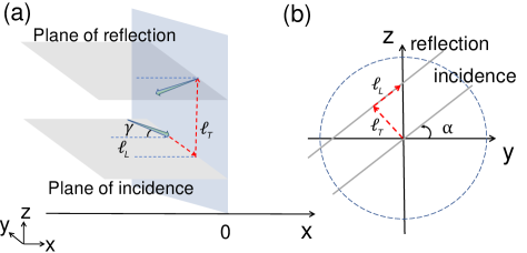
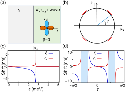
Let us first describe the basic setup of side incidence configuration. As illustrated in Fig. 1(a), we consider a flat NS interface. The left side () is occupied by the normal (N) medium (e.g., simple metal or vacuum). The right side () is occupied by the superconducting (S) medium. The system is extended in the and directions, so momenta and are conserved during scattering at the interface. Consider an electron beam incident from the N side. The incident plane is defined by the beam and the interface normal vector. We use the angle
| (1) |
to specify the incident plane. As shown in Fig. 1(b), is the angle of incident plane measured from the axis. Inside the incident plane, the incident angle of the beam is denoted by [see Fig. 1(a)], and corresponds to the case of normal incidence.
The essential physics of scattering at the NS interface can be described by the Bogoliubov-de Gennes (BdG) equation [30, 31]:
| (2) |
where is the kinetic energy term (we set ), is the Fermi energy, is the superconducting pair potential, is the Heaviside step function indicating that the pairing occurs on the S side, and with denoting a potential energy difference between the two sides and denoting a possible interface barrier potential. For side incidence configuration, the principal axis of the S side is along . For unconventional pairings, the pair potential should have strong dependence on and , and we will neglect its dependence. For example, for the chiral -wave pairing, we write , where parameters and . In this model, we take isotropic Fermi surfaces. In practice, unconventional superconductors often have anisotropic Fermi surfaces. We will discuss effects of anisotropic Fermi surface later in Sec. VII.
III analytic results
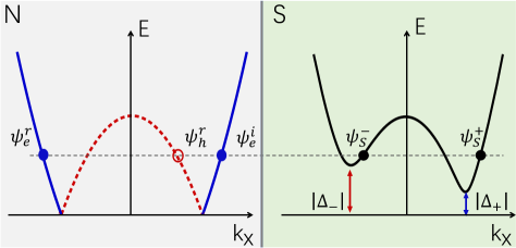
Before performing calculations, we first analyze states that are involved in a scattering. Since the momentum parallel to the interface is conserved, in our model, there will be five states involved (see Fig. 2): incident electron state , reflected electron state , reflected hole state , and two transmitted states and . In Fig. 2, one can see that is an electron-like quasiparticle state, whereas is a hole-like quasiparticle state. It should be noted that the superconducting gaps around the locations of and could be different, due to the dependence of for unconventional pair potential. We denote the two gaps as and , respectively (see Fig. 2). They generally depend on the energy and momentum of the incident electron. We define their phase angles as
| (3) |
For the case illustrated in Fig. 2, and are propagating modes in S. When the excitation energy is below (), () will become an evanescent mode.
Now, for a given incident electron state , we can write down the corresponding scattering state for the BdG equation (2):
| (4) |
where is the amplitude for normal (Andreev) reflection, and are the two amplitudes for transmissions into states.
The three states in the N region can be written as
| (7) | |||||
| (10) | |||||
| (13) |
with and . Here, we assume , so corrections to of order are neglected. From the configuration in Fig. 1, we have the relation .
In the S region, the basis states (not normalized) can be written as
| (14) |
Here, have been defined in Eq. (3) which are phases of pair potential, and
| (15) |
and the momentum , with
| (16) |
In the treatment, we take the weak coupling limit, with . Meanwhile, the magnitudes of and can be comparable. One notes that for , is a positive (real) number, whereas for , becomes complex.
The boundary conditions for the BdG equation at the interface are derived from the quasiparticle current conservation [30, 32]. They take the form of
| (17) | ||||
The scattering amplitudes (’s and ’s) can be solved from Eq. (17) by substituting Eq. (4). The information of the spatial shift in Andreev reflection is encoded in the scattering amplitude . After straightforward calculations, we obtain
| (18) |
where we define dimensionless parameters and
| (19) |
Based on the results in Ref. [24, 33], the spatial shift for the Andreev reflected hole beam can be calculated from
| (20) |
with . The shift depends on the phase of , not its magnitude. It is customary to decompose the shift vector into the longitudinal component inside the incident plane and the transverse component normal to the plane (see Fig. 1). In the present setup, we have
| (21) |
and
| (22) |
Now, to obtain the phase angle , by using the result in Eq. (18), we find
| (23) |
where
| (24) |
Since and may have different values, besides the two cases in Eq. (23), we have another two cases: when , we find
| (25) |
and when ,
| (26) |
Before proceeding, let’s make a comparison with top incidence configuration. In that case, one always has the equality , so essentially the subscripts can be dropped in quantities involved in the formulas above. This will greatly simplify the result. One can deduce that
| (27) |
where we define , , and . This recovers the previous result in Ref. [25].
Back to side incidence configuration considered here, generally, we have . Then, the resulting expressions of , i.e., Eqs. (23-26), are more complicated. Nevertheless, if we restrict to the regime where is the largest energy scale, i.e., with , and not close to , then we have , , , and , so that
| (28) |
In this regime, the expression for is simplified to
| (29) |
This is a very nice result. We have the following observations. First, the result depends on the state but not state. This can be intuitively understood, because for large , is largely separated in momentum from , , and states, so it has little influence on Andreev reflection. Second, in Eq. (29), has two contributions when is below the superconducting gap. The first contribution originates from the phase of pair potential. The second contribution originates from the evanescent character of state in this case. Indeed, previous studies showed that evanescent modes play a critical role in generating the spatial shift. These are the two sources of the phase change between the incident electron and the Andreev reflected hole. Third, when the excitation energy is above the gap, we only have the contribution. This is because state now becomes a propagating mode, which then does not contribute a phase change.
In the following sections, we will apply the above formulas to three different types of pair potentials on the S side.
IV s-wave pairing
Let’s first apply the results in Sec. III to the case of conventional -wave pair potential. Since this case is isotropic, the result for side incidence should be the same as that for top incidence. The purpose of the discussion here is mainly for completeness and also to provide a reference to which the results of unconventional pairing cases can be compared.
For a -wave pair potential, we model being a real constant parameter. By using the result in Sec. III, especially the analysis around Eq. (27), we find that the two components of the shift are given by
| (30) |
| (31) |
for ; and
| (32) |
for . In the above expression, and .
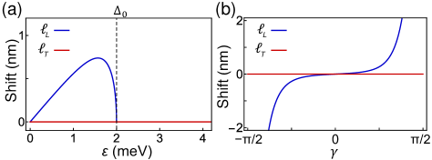
In this case, the pair potential does not have a nontrivial phase variation, so a nonzero shift has to come from the evanescent mode contribution, which requires . Clearly, the result should not depend on angle , due to isotropy of the model. One observes that the transverse component of the shift vanishes. This can be readily understood by noting that the system always has a mirror symmetry with respect to the incident plane. Regarding the longitudinal shift , it is an odd function of [see Fig. 3(b)], as is odd in . From Eq. (31), a finite would require a finite or . We also note that a large which dominates over and would suppress the value of . This is because for such case, according to the discussion around Eq. (28), becomes a -independent number ( for -wave). Then the shift from Eq. (20) should vanish. These results are consistent with the previous studies for -wave case in the top incidence configuration [24, 25].
V chiral p-wave pairing
Next, we consider the case with a chiral -wave superconductor. The pair potential on S side is modeled as , where denotes the chirality. For such a chiral pair potential, the two gaps are the same, regardless of the angles and . Here, we focus on the regime with . By using Eq. (29), the expressions of the anomalous shift can be obtained as
| (33) |
for longitudinal shift, and
| (34) |
for transverse shift. Here, , and we define .
We have the following observations on these results. First, the basic structure of the expressions follow the discussion at the end of Sec. III. Namely, for , the shift has two contributions, the first is from the phase of pair potential, and the second is from the evanescent character of mode ; for , there is only one contribution, from the pairing phase. This feature holds for both longitudinal and transverse shifts.
Second, since the phase of pair potential depends on the chirality , the pairing phase contribution in the shift contains the factor. In comparison, the evanescent mode contribution for does not depend on chirality. For , both and are proportional to , so the shift would flip sign if the chirality of the pair potential is reversed.
Third, we note that at , i.e., when the incident plane coincides with the - plane, vanishes because the system has a mirror symmetry with respect to the incident plane. Meanwhile, for , the evanescent mode contribution vanishes due to its dependence, and we find a particularly simple result
| (35) |
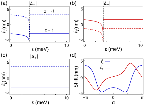
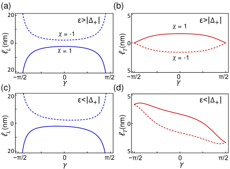
which is independent of the excitation energy . For , is an even function of , whereas is an odd function. In Figs. 4(a,b), we plot the variation of the shift components versus at . One can see that the evanescent mode contribution for gives a large contribution close to the superconducting gap.
Finally, regarding the dependence on the incident angle , we note that the pairing phase contribution is an even function of , whereas the evanescent mode contribution is an odd function. It follows that for , the curves for and are symmetric about [see Fig. 5(a,b)]. In comparison, for , the curves are generally neither symmetric nor antisymmetric [see Fig. 5(c,d)], due to the presence of both contributions. Interestingly, for , i.e., the normal incidence case, we have a simple result: the shift should be along the direction, with
| (36) |
which is proportional to the chirality of pairing and independent of the excitation energy.
VI d-wave pairing
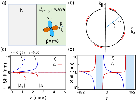
The third model we consider is that with a -wave pair potential, which we take as . Here, is the angle between the wave and the normal direction of the interface (-axis). For example, the typical cases with and are illustrated in Figs. 6 and 7. In the following analysis, we again focus on the regime with .
Using Eq. (29), we obtain the following analytical expressions for the anomalous shift components:
| (37) | |||||
| (38) |
for , and
| (39) |
for . Here, we have . Typical behaviors of the two shift components versus model parameters have been shown in Figs. 6 to 8. We have the following observations.
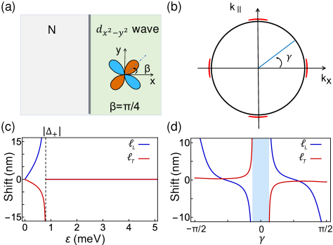
First, since the pair potential here is real, there is no pairing phase contribution to the shift, and only evanescent mode contribution exists. This explains why the shift vanishes when , a behavior distinct from the chiral -wave case we discussed in the preceding section. Note that -wave pair potential has nodes, where the superconducting gap vanishes. This indicates that for a finite excitation energy and large , there always exist some range of incident angle in which is satisfied and therefore the shift is suppressed. For example, for the case with (see Fig. 6), vanishes at the two nodes located at . This leads to two suppressed zones [marked by the shaded region in Fig. 6(d)] for the incident angle when it varies from to . For , the nodes are shifted, which also shift the locations of the suppressed zones [see Fig. 8(d)]. In the case with , there is only one suppressed zone around [see Fig. 7(d)]. By detecting the suppressed zones, one can in principle map out the locations of the nodes.
Second, regarding the dependence on the angle of incident plane, from Eqs. (37-38), we see that is an even function, whereas is an odd function. This is similar to the chiral -wave case in Sec. V. It follows that the transverse shift vanishes when . Nevertheless, it can be sizable for when the excitation energy is just below the gap [see e.g., Fig. 8(c)].
Third, when , the expressions for the two shift components are simplified as
| (40) |
| (41) |
with . They have opposite signs, and they are both odd functions of the incident angle , as is odd in and is even in . These behaviors are illustrated in Fig. 6(d). For another special case with , we have the following simplified expressions:
| (42) |
| (43) |
with . One notes that in this case, again, the two components are odd functions of the incident angle [see Fig. 7(d)], because is odd in (through ). For a general angle , the shift does not have a definite parity with respect to , as shown in Fig. 8(d).
Finally, for normal incidence (with ), the formula is reduced to
| (44) |
where is the Heaviside step function, and . This shift is along the direction and can be nonzero for the general case when is not an integer multiple of .
VII Discussion and Conclusion
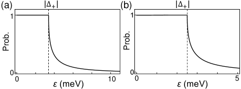
The anomalous spatial shift in Andreev reflection is connected with the phase of the reflection amplitude . The magnitude of , on the other hand, determines the probability of Andreev reflection. For large , this probability is typically close to unity when is below the gap and decays with when is above the gap [30]. For example, the variation of probability versus is plotted in Fig. 9. for the two cases with chiral -wave pairing and with -wave pairing, which confirms the above point.
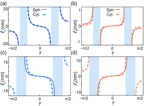
In our model, we used an isotropic Fermi surface. To investigate the effects of Fermi surface anisotropy, we change the normal state Hamiltonian for the S region to be , which is dispersionless along the direction. This gives a cylindrical Fermi surface for the S side, representing a very strong anisotropy. For this modified model, analytic results are too complicated to analyze. Nevertheless, we may proceed numerically. As shown in Fig. 10(a,b), we find that for small angle of the incident plane, the results for the modified model with cylindrical Fermi surface agree very well with those for spherical Fermi surface. This can be understood by noting that when , the scattering involves only the states around the Fermi circle with in S, which makes little difference between cylindrical and spherical Fermi surfaces. With increased , the results for the cylindrical Fermi surface model does show quantitative difference from the spherical model, but the qualitative features are maintained. For example, in Fig. 10(c,d), we compare the results of the two models for in the case of -wave pairing. We see that the two models share similar features, such as existence of suppressed zones, parity with respect to incident angle, and trend of variation against other parameters.
Regarding experimental detection, the most straightforward way is to prepare a collimated electron beam and let it hit the surface of the superconductor (N side is vacuum in this case), just like the setup of the electron microscope. Then, we detect the Andreev reflected hole beam. By comparing the trajectories of the incident and the reflected beams, one can extract the shift at the surface during scattering. Our estimation here shows that the shift can reach the magnitude of tens of nanometers, which should be detectable with current technology. In a NS junction formed by a conventional metal and a superconductor, the shift at the interface may lead to a voltage signal in the transverse direction on the N side close to the interface, when an electric current is driven through the junction. For example, for the junction with a chiral -wave superconductor with interface coinciding with the - plane, according to Eq. (36), the shift should lead to a voltage drop in the direction and its sign is determined by the chirality of the pair potential. In addition, the shift may be accumulated by designing heterostructures in which an electron beam can undergo multiple scattering [14, 26].
In conclusion, we have investigated the anomalous shift in Andreev reflection at an NS interface in the side incidence configuration. The results show rich and distinct behaviors for different types of pairing. For chiral wave pairing, there are two contributions. The pairing phase contribution which is proportional to chirality and the evanescent mode contribution which is independent of chirality. For excitation energy above the pairing gap, the evanescent mode contribution vanishes, whereas the pairing phase contribution persists, leading to a particularly simple result. For -wave pairing, only the evanescent mode contribution exists, so the shift vanishes for excitation energy above the gap. Around the nodes of the superconducting gap, there are suppressed zones where the shift vanishes. This offers a way to map out the superconducting nodes. The dependence of the shift on excitation energy, incident angle, and other system parameters are analyzed. These findings deepen our understanding of the fundamental scattering process at the NS interface, offer new methods to characterize superconductors, and may be useful for designing novel superconducting devices.
References
- Bliokh and Aiello [2013] K. Y. Bliokh and A. Aiello, Journal of Optics 15, 014001 (2013).
- Bliokh et al. [2015] K. Y. Bliokh, F. J. Rodríguez-Fortuño, F. Nori, and A. V. Zayats, Nature Photonics 9, 796 (2015).
- Ling et al. [2017] X. Ling, X. Zhou, K. Huang, Y. Liu, C.-W. Qiu, H. Luo, and S. Wen, Reports on Progress in Physics 80, 066401 (2017).
- Goos and Hänchen [1947] F. Goos and H. Hänchen, Annalen der Physik 436, 333 (1947).
- F. I. Fedorov [1955] D. A. F. I. Fedorov, Nauk SSSR 105, 465 (1955).
- Imbert [1972] C. Imbert, Phys. Rev. D 5, 787 (1972).
- Ban and Chen [2023] Y. Ban and X. Chen, Phys. Rev. A 108, 042218 (2023).
- Miller and Ashby [1972] S. C. Miller and N. Ashby, Phys. Rev. Lett. 29, 740 (1972).
- Fradkin and Kashuba [1974a] D. M. Fradkin and R. J. Kashuba, Phys. Rev. D 9, 2775 (1974a).
- Fradkin and Kashuba [1974b] D. M. Fradkin and R. J. Kashuba, Phys. Rev. D 10, 1137 (1974b).
- Spector et al. [1990] J. Spector, H. L. Stormer, K. W. Baldwin, L. N. Pfeiffer, and K. W. West, Applied Physics Letters 56, 1290 (1990).
- Molenkamp et al. [1990] L. W. Molenkamp, A. A. M. Staring, C. W. J. Beenakker, R. Eppenga, C. E. Timmering, J. G. Williamson, C. J. P. M. Harmans, and C. T. Foxon, Phys. Rev. B 41, 1274 (1990).
- Dragoman and Dragoman [1999] D. Dragoman and M. Dragoman, Progress in quantum electronics 23, 131 (1999).
- Beenakker et al. [2009] C. W. J. Beenakker, R. A. Sepkhanov, A. R. Akhmerov, and J. Tworzydło, Phys. Rev. Lett. 102, 146804 (2009).
- Chen et al. [2011] X. Chen, J.-W. Tao, and Y. Ban, The European Physical Journal B 79, 203 (2011).
- Sharma and Ghosh [2011] M. Sharma and S. Ghosh, Journal of Physics: Condensed Matter 23, 055501 (2011).
- Wu et al. [2011] Z. Wu, F. Zhai, F. M. Peeters, H. Q. Xu, and K. Chang, Phys. Rev. Lett. 106, 176802 (2011).
- Jiang et al. [2015] Q.-D. Jiang, H. Jiang, H. Liu, Q.-F. Sun, and X. C. Xie, Phys. Rev. Lett. 115, 156602 (2015).
- Yang et al. [2015] S. A. Yang, H. Pan, and F. Zhang, Phys. Rev. Lett. 115, 156603 (2015).
- Jiang et al. [2016] Q.-D. Jiang, H. Jiang, H. Liu, Q.-F. Sun, and X. C. Xie, Phys. Rev. B 93, 195165 (2016).
- Wang and Jian [2017] L. Wang and S.-K. Jian, Phys. Rev. B 96, 115448 (2017).
- Chattopadhyay et al. [2019] U. Chattopadhyay, L.-k. Shi, B. Zhang, J. C. W. Song, and Y. D. Chong, Phys. Rev. Lett. 122, 066602 (2019).
- Liu et al. [2020] Y. Liu, Z.-M. Yu, C. Xiao, and S. A. Yang, Phys. Rev. Lett. 125, 076801 (2020).
- Liu et al. [2017] Y. Liu, Z.-M. Yu, and S. A. Yang, Phys. Rev. B 96, 121101 (2017).
- Yu et al. [2018] Z.-M. Yu, Y. Liu, Y. Yao, and S. A. Yang, Phys. Rev. Lett. 121, 176602 (2018).
- Liu et al. [2018] Y. Liu, Z.-M. Yu, H. Jiang, and S. A. Yang, Phys. Rev. B 98, 075151 (2018).
- Sigrist and Ueda [1991] M. Sigrist and K. Ueda, Rev. Mod. Phys. 63, 239 (1991).
- Tsuei and Kirtley [2000] C. C. Tsuei and J. R. Kirtley, Rev. Mod. Phys. 72, 969 (2000).
- Bergeret et al. [2005] F. S. Bergeret, A. F. Volkov, and K. B. Efetov, Reviews of Modern Physics 77, 1321 (2005).
- Blonder et al. [1982] G. E. Blonder, M. Tinkham, and T. M. Klapwijk, Phys. Rev. B 25, 4515 (1982).
- de Gennes [1999] P.-G. de Gennes, Superconductivity of Metals and Alloys, Advanced Book Classics (Advanced Book Program, Perseus Books, Reading, Mass, 1999).
- Kashiwaya and Tanaka [2000] S. Kashiwaya and Y. Tanaka, Reports on Progress in Physics 63, 1641 (2000).
- Yu et al. [2019] Z.-M. Yu, Y. Liu, and S. A. Yang, Frontiers of Physics 14, 1 (2019).