Particle approximation for a conditional McKean–Vlasov stochastic differential equation

Abstract

In this paper, we construct a type of interacting particle systems to approximate a class of stochastic different equations whose coefficients depend on the conditional probability distributions of the processes given partial observations. After proving the well-posedness and regularity of the particle systems, we establish a quantitative convergence result for the empirical measures of the particle systems in the Wasserstein space, as the number of particles increases. Moreover, we discuss an Euler–Maruyama scheme of the particle system and validate its strong convergence. A numerical experiment is conducted to illustrate our results.

AMS subject classification: 60G25, 60G35, 60H35

Key words: conditional McKean–Vlasov SDE, conditional propagation of chaos, synchronous coupling, error estimates in Wasserstein space, Euler–Maruyama scheme.

1 Introduction

This paper is concerned with a conditional McKean–Vlasov stochastic differential equation (CMVSDE) in a completed probability space $(\Omega,\mathcal{F},\mathbb{P})$:

$$\left\{\begin{aligned} X_{t}&=x+\int_{0}^{t}b(X_{s},\pi_{s})\,\mathrm{d}s+\int_{0}^{t}\sigma_{1}(X_{s},\pi_{s})\,\mathrm{d}W_{s}+\int_{0}^{t}\sigma_{2}(X_{s},\pi_{s})\,\mathrm{d}B_{s},\\[8.5359pt] Y_{t}&=\int_{0}^{t}h(X_{s},\pi_{s})\,\mathrm{d}s+B_{t},\qquad\quad\text{with }\ \pi_{s}(\cdot)=\mathbb{P}\big{[}{X}_{s}\in\cdot\,|\mathcal{F}_{s}^{Y}\big{]},\end{aligned}\right.$$ (1.1)

where $x\in\mathbb{R}^{n}$, $\mathcal{F}_{t}^{Y}=\sigma\{Y_{s}:s\leq t\}$, and $(B,W)$ is a standard Brownian motion. The process $Y$ serves as observations, resulting in a conditional law $\pi$ of $X$ that is involved in the dynamics of $X$. We remark that when $h$ vanishes, the equation (1.1) becomes the so-called McKean–Vlasov SDE with common noise which has been extensively studied in the literature, see e.g. [8, 15, 5], and [12] for some recent progress. As $h$ emerges and relies on $X$, the increased reliance of the observation process $Y$ on the state $X$ substantially amplifies the nonlinearity within the dynamics. Very recently, the well-posedness of (1.1) is obtained by Buckdahn, Li, and Ma [4] by employing Banach’s fixed point theorem and a localization technique. The study on (1.1) is motivated by applications in mathematical finance and stochastic control. For instance, Ma, Sun, and Zhou [24] formulated a linear form of CMVSDE (1.1) based on the Kyle–Back equilibrium model; Buckdahn, Li, and Ma [3] studied a control problem arising in the mean-field game, in which the coefficients of the controlled dynamics linearly depend on the conditional law of the state.

In this paper, we aim to construct a particle system to approximate CMVSDE (1.1). To approximate the conditional law $\pi$ in an appropriate way, we draw upon the methodology from nonlinear filtering theory and introduce the reference probability measure $\mathbb{Q}$ by the Girsanov transformation:

$$\frac{\mathrm{d}\mathbb{Q}}{\mathrm{d}\mathbb{P}}\Big{|}_{t}=\frac{1}{L_{t}}:=\exp\bigg{(}-\int_{0}^{t}h(X_{s},\pi_{s})\mathrm{d}Y_{s}+\frac{1}{2}\int_{0}^{t}\left|h(X_{s},\pi_{s})\right|^{2}\mathrm{d}s\bigg{)}.$$

As a result, the observation process $Y$ is a standard Brownian motion under $\mathbb{Q}$, and by Bayes’ formula (or the Kallianpur–Striebel formula), one can write the conditional law $\pi$ defined in (1.1) as

$$\pi_{s}(\cdot)=\mathbb{P}[{X}_{s}\in\cdot\,|\mathcal{F}_{s}^{Y}]=\frac{\mathbb{E}^{\mathbb{Q}}[{L}_{s}\bm{1}_{{X}_{s}\in\,\cdot}\,|\mathcal{F}_{s}^{Y}]}{\mathbb{E}^{\mathbb{Q}}[{L}_{s}|\mathcal{F}_{s}^{Y}]}.$$ (1.2)

Based on this transformation, we introduce a particle system $\{(X^{i,N},L^{i,N})\}_{i=1}^{N}$ on $(\Omega,\mathbb{Q},\mathcal{F})$:

$$\left\{\begin{aligned} X_{t}^{i,N}&=x+\int_{0}^{t}(b-\sigma_{2}h)(X_{s}^{i,N},\pi_{s}^{N})\mathrm{d}s+\int_{0}^{t}\sigma_{1}(X_{s}^{i,N},\pi_{s}^{N})\mathrm{d}W_{s}^{i}+\int_{0}^{t}\sigma_{2}(X_{s}^{i,N},\pi_{s}^{N})\mathrm{d}Y_{s},\\[8.5359pt] L_{t}^{i,N}&=1+\int_{0}^{t}h(X_{s}^{i,N},\pi_{s}^{N})L_{s}^{i,N}\mathrm{d}Y_{s},\\[8.5359pt] \pi_{s}^{N}&=\frac{\sum_{i=1}^{N}{L}^{i,N}_{s}\delta_{X_{s}^{i,N}}}{\sum_{i=1}^{N}{L}^{i,N}_{s}}=\sum\limits_{i=1}^{N}{w}_{s}^{i}\,\delta_{{X}_{s}^{i,N}}\quad\text{with}\quad{w}^{i}_{s}=\frac{{L}^{i,N}_{s}}{\sum_{i=1}^{N}{L}^{i,N}_{s}},\end{aligned}\right.$$ (1.3)

where $\{W^{i}\}_{i=1}^{N}$ are independent Brownian motions under $\mathbb{Q}$ and independent of $Y$. Intuitively, the process $L^{i}$ plays a role of a likelihood weight assigned to the path $X^{i}$ that represents the probability of that path being sampled from the conditional law. We can illustrate the validity of this model from two perspectives. First, if the coefficient $h$ is a constant, then $\pi_{t}^{N}=\frac{1}{N}\sum_{i=1}^{N}\delta_{X_{t}^{i,N}}$ is an unweighted empirical measure and converges, as $N\to\infty$, to the conditional law of a McKean–Vlasov process with common noise (cf. [8]). Second, if the coefficients are all independent of the distribution $\pi$, then (1.3) becomes a standard model for particle filter, such as in [7], Crisan, Gaines and Lyons construct a special sequence of branching particle systems to the solution of the Zakai equation; and in [9], Crisan and Lyons studies use branching particle systems to study the solution of Kushner–Stratonovitch equation; and in [29], some particle stability results are obtained by Whiteley. However, in its full generality, the system (1.3) is highly coupled and nonlinear; in particular, it is not Lipschitz even the coefficients are all bounded and smooth. As an indispensable intermediate step, we prove the uniqueness and existence of strong solutions to the particle system (1.3) by combining the multiplier method, the tightness argument, and the Yamada–Watanabe theorem.

In this paper, we establish the conditional propagation of chaos (CPoC) property of the particle system (1.3). Specifically, we prove that, as $N$ increases, the weighted empirical measure $\pi_{t}^{N}$ converges to the conditional law $\pi_{t}$ in our target equation (1.1); moreover, we provide a quantitative characterization for the convergence rate in terms of the Wasserstein distance. We remark that there are many relevant results in the literature. For instance, Zheng [30] applied CPoC to solve a class of quasilinear equations of parabolic type; Kurtz and Xiong [16, 17, 18] constructed a sequence of weighted empirical measures from a particle system to approximate a class of nonlinear SPDE and verify the convergence in the weak topology; Coghi and Flandolli [6] established the CPoC property of the particle system with common space-dependent noise; and Erny, Löcherbach, and Loukianova [10] considered jumping particle systems, among others. To our knowledge, our results differ significantly from existing ones in at least two aspects. First, the particle system (1.3) is not covered by the existing models and its well-posedness result obtained here is new. Second, we derive a quantitative CPoC in terms of the Wasserstein distance, whereas a related paper [17] proved the convergence in law without convergence rate and under stronger regularity requirements on the coefficients. Technically, we develop a multiplier method to deal with the well-posedness and asymptotic behavior of non-Lipschitz particle systems. In contrast to the localization technique used in [4, 17], our method stands out in its capacity to notably streamline calculations but also to generate new quantitative estimates.

It is worth noting that the CMVSDE (1.1) is closely related to the optimal control problem with partial observation (see e.g. [1, 25, 27, 28, 22]). In particular, in recent years, there has been growing interest in the problem of mean-field control (MFC) and mean-field game (MFG) with partial observation (see e.g. [20, 21, 19, 26, 2, 11]). What’s more, noticing that $\pi_{t}$ in (1.1) satisfies the Zakai equation, our approximation result may be helpful to compute some stochastic control problem driven by Zakai equation (see e.g. [1, 23]) since our work is associated with particle filters, which use particle systems to approximate the solutions in nonlinear filtering problems.

The rest of this paper is structured as follows: In Section 2, we present the main results including well-posedness and CPoC property of (1.3), and error bound of the fully discretization scheme. Auxiliary lemmas are proved in Section 3. Section 4 is devoted to the proof of the main results. The analysis is confirmed by numerical examples in Section 5.

For convenience, in what follows we shall assume $\sigma_{2}=0$ in (1.1). The case of $\sigma_{2}\neq 0$ is known as the “correlated noise case” in the nonlinear filtering theory, which is well-understood and without substantial difficulties, although technically slightly more tedious (see e.g. [4]). We prefer not to pursue such complexity in this paper but focus on the conditional McKean-Vlasov nature instead, that is, we set that $\sigma_{1}=\sigma$ and $\sigma_{2}=0$.

2 Main results

Throughout this paper, we assume that the coefficients $\phi=(b,\sigma,h):\mathbb{R}^{n}\times\mathcal{P}_{1}(\mathbb{R}^{n})\rightarrow\mathbb{R}^{n}\times\mathbb{R}^{n\times m}\times\mathbb{R}^{k}$ is bounded and globally Lipschitz continuous: there is a constant $K\geq 0$ such that

$$|\phi(x,\mu)|\leq K\quad\text{and}\quad|\phi(x,\mu)-\phi(y,\mu^{\prime})|\leq K(|x-y|+W_{1}(\mu,\mu^{\prime})),$$

where $W_{1}(\cdot,\cdot)$ denotes the $1$-Wasserstein distance of probability measure:

$$W_{1}(\mu_{1},\mu_{2}):=\inf\big{\{}\mathbb{E}|\xi_{1}-\xi_{2}|:\mathrm{law}(\xi_{1})=\mu_{1},\,\mathrm{law}(\xi_{2})=\mu_{2}\big{\}}.$$

2.1 Conditional propagation of chaos

First, we establish the well-posedness of the particle system (1.3).

Theorem 2.1.

The particle system (1.3) admits a unique strong solution $\{(X^{i,N},L^{i,N})\}_{i=1}^{N}$.

Next we use the particle system (1.3) to approximate the signal $X$ in (1.1) and the conditional measure $\pi$ in (1.2). To do this, we apply the synchronous coupling technique to generate $\{\bar{X}^{i},\bar{L}^{i}\}_{i=1}^{N}$, which is the solution to SDE (1.1) with the driven terms replaced by the Brownian motion $\{W^{i},Y\}_{i=1}^{N}$ appearing in the particle system (1.3). Since $\{W^{i},Y\}_{i=1}^{N}$ is a standard Brownian motion, we know that for all $1\leq i\leq N$, the conditional distribution of the synchronous coupling signal $\mathscr{L}^{\mathbb{P}}(\bar{X}^{i}_{t}|\mathcal{F}^{Y}_{t})$ is identical to the conditional distribution of the original signal $\pi$ defined in (1.2). For any fixed $N\in\mathbb{N}_{+}$, we define for all $s\in[0,T]$

$$\bar{\pi}_{s}^{N}=\frac{\sum_{i=1}^{N}\bar{L}_{s}^{i}\delta_{\bar{X}_{s}^{i}}}{\sum_{i=1}^{N}\bar{L}_{s}^{i}}=\sum\limits_{i=1}^{N}\bar{w}_{s}^{i}\,\delta_{\bar{X}_{s}^{i}}\quad\text{with}\quad\bar{w}^{i}_{s}=\frac{\bar{L}^{i}_{s}}{\sum_{i=1}^{N}\bar{L}^{i}_{s}}.$$ (2.1)

We have the following approximation theorem.

Theorem 2.2.

There is a constant $C=C(K,T,n)$ such that

$$\mathbb{E}^{\mathbb{Q}}\Big{[}\max_{t\in[0,T]}\big{|}X_{t}^{i,N}-\bar{X}^{i}_{t}\big{|}^{2}\Psi_{t}\Big{]}\leq CN^{-\frac{8}{7n+8}},\quad\quad\forall i=1,2,...,N,$$

where $n$ is the dimension of synchronous coupling signal $\bar{X}^{i}$ and the multiplier is defined by

$$\Psi_{t}=\exp\bigg{\{}-\alpha N\sum\limits_{k=1}^{N}\int_{0}^{t}\left[\frac{1}{N^{2}}+\Big{(}\big{|}w_{s}^{k}\big{|}^{2}+\big{|}\bar{w}_{s}^{k}\big{|}^{2}\Big{)}\Big{(}1+\big{|}X_{s}^{k,N}\big{|}^{2}\Big{)}\right]\mathrm{d}s\bigg{\}},$$

with $\alpha=\alpha(K,T)$ and the random normalized weights ${w}^{i}_{s}$ and $\bar{w}^{i}_{s}$ given by (1.3) and (2.1).

Remark 2.1.

If $h$ is a constant or all the coefficients are independent of $\pi$, then multiplier $\Psi_{t}$ can be just chosen as $\Psi_{t}=e^{-\alpha t}$ with $\alpha=\alpha(K,T)>0$. Then we can get that

$$\mathbb{E}^{\mathbb{Q}}\Big{[}\max_{t\in[0,T]}\big{|}X_{t}^{i,N}-\bar{X}^{i}_{t}\big{|}^{2}\Big{]}\leq CN^{-\frac{8}{7n+8}},\quad\quad\forall i=1,2,...,N,$$

where $C=C(K,T,n)$.

In view of Theorem 2.2, we can get the mean convergence rate of $\mathbb{E}^{\mathbb{Q}}[|X_{t}^{i}-\bar{X}^{i}_{t}|^{2}]$ as follows by estimating multipliers.

Corollary 2.1.

For all $i=1,2,...,N$ and $\beta>0$, there exists $C=C(\beta,K,T,n)$ such that

$$\mathbb{E}^{\mathbb{Q}}\Big{[}\max\limits_{t\in[0,\tau_{\beta}\wedge T]}\big{|}X_{t}^{i,N}-\bar{X}^{i}_{t}\big{|}^{2}\Big{]}\leq CN^{-\frac{8}{7n+8}},$$

where the stopping time is defined as

$$\tau_{\beta}:=\inf\bigg{\{}t:N\sum\limits_{k=1}^{N}\int_{0}^{t}\left[\frac{1}{N^{2}}+\Big{(}\big{|}w_{s}^{k}\big{|}^{2}+\big{|}\bar{w}_{s}^{k}\big{|}^{2}\Big{)}\Big{(}1+\big{|}X_{s}^{k,N}\big{|}^{2}\Big{)}\right]\mathrm{d}s>\beta\bigg{\}},$$

with

$$\mathbb{Q}[\tau_{\beta}>T]>1-\frac{C}{\beta}.$$

Furthermore, it holds that

$$\max\limits_{t\in[0,T]}\mathbb{E}^{\mathbb{Q}}\Big{[}W_{1}\big{(}\pi^{N}_{t},\pi_{t}\big{)}^{2}\Big{]}+\mathbb{E}^{\mathbb{Q}}\Big{[}\max\limits_{t\in[0,T]}\big{|}X_{t}^{i,N}-\bar{X}^{i}_{t}\big{|}^{2}\Big{]}\leq C\bigl{|}\ln(N)\bigr{|}^{-\frac{1}{2p}},\quad\quad\forall p>1,$$

where $C=C(K,T,n,p)$, $\pi_{t}^{N}$ is the empirical measure defined in (1.3) and $\pi_{t}$ is the target measure defined in (1.2).

Remark 2.2.

The convergence rate $\mathcal{O}(|\ln(N)|^{-\frac{1}{2}+})$ results from the fact that the inverse of multiplier $\Psi^{-1}$ is not bounded, and even not integrable in general, which makes the estimation of convergence rate become intractable. However, we observe that $\ln(\Psi^{-1})$ is integrable, which allows us to get the convergence rate $\mathcal{O}(|\ln(N)|^{-\frac{1}{2}+})$. Although this convergence rate is much slower compared to the classical result, it seems to be the first result in regard to the strong convergence rate for the mean-field particle filters. Moreover, our numerical scheme works very well in some examples even in the cases when coefficients are not bounded (see Section 5).

2.2 Sequential importance sampling: full discretization

Next, we use the sequential importance sampling to fully discretize the SDE (1.1), which is a Monte Carlo algorithm based on the CPoC property and the Euler scheme. To approximate the random weight $\{\bar{L}^{i}\}_{i=1}^{N}$, it is equivalent to consider the random normalized weight $\{\bar{w}^{i}\}_{i=1}^{N}$ define in (2.1). By Ito’s formula, the dynamic of $\bar{w}_{t}^{i}$ is governed by

$$\mathrm{d}\bar{w}_{t}^{i}=\bar{w}_{t}^{i}\,H\left(\bar{X}_{t}^{i},\bar{\pi}_{t}^{N}\right)\mathrm{d}t+\bar{w}_{t}^{i}\,M^{\text{T}}\left(\bar{X}_{t}^{i},\bar{\pi}_{t}^{N}\right)\mathrm{d}Y_{t},\qquad\bar{w}^{i}_{0}=1,$$ (2.2)

where the coefficient $(M,H):\mathbb{R}^{n}\times\mathcal{P}_{1}(\mathbb{R}^{n})\rightarrow\mathbb{R}^{k}\times\mathbb{R}$ is the function satisfying

$$M(x,\pi)=h(x,\pi)-\int h(x,\pi)\pi(\mathrm{d}x),$$

and

$$H(x,\pi)=\Big{|}\int h(x,\pi)\pi(\mathrm{d}x)\Big{|}^{2}-h^{\text{T}}(x,\pi)\int h(x,\pi)\pi(\mathrm{d}x).$$

Then the full discretization for the synchronous coupling signal $\bar{X}^{i}$ and for the random normalized weight $\bar{w}^{i}$ in (2.2) is: $\forall 1\leq i\leq N$,

$$\left\{\begin{aligned} &\mathrm{d}X_{t}^{i,\Delta}=b\big{(}X_{\theta(t,\Delta)}^{i,\Delta},\pi_{\theta(t,\Delta)}^{N,\Delta}\big{)}\mathrm{d}t+\sigma\big{(}X_{\theta(t,\Delta)}^{i,\Delta},\pi_{\theta(t,\Delta)}^{N,\Delta}\big{)}\mathrm{d}W_{t}^{i},\qquad X_{0}^{i,\Delta}=x,\\[8.5359pt] &\mathrm{d}w_{t}^{i,\Delta}=w_{t}^{i,\Delta}H\big{(}X_{\theta(t,\Delta)}^{i,\Delta},\pi_{\theta(t,\Delta)}^{N,\Delta}\big{)}\mathrm{d}t+w_{t}^{i,\Delta}M^{\text{T}}\big{(}X_{\theta(t,\Delta)}^{i,\Delta},\pi_{\theta(t,\Delta)}^{N,\Delta}\big{)}\mathrm{d}Y_{t},\qquad w^{i,\Delta}_{0}=1,\end{aligned}\right.$$ (2.3)

where

• $\Delta\in(0,T)$ is the size of time step, and $\theta:[0,T]\times(0,T)\rightarrow[0,T]$ is a measurable function such that

  $$\theta(t,\Delta)=\Big{\lfloor}\frac{t}{\Delta}\Big{\rfloor}\Delta,$$

  with $\lfloor\cdot\rfloor$ being the floor function;

• the empirical measure with random weights is defined by

  $$\pi_{t}^{N,\Delta}=\sum\limits_{i=1}^{N}w_{t}^{i,\Delta}\,\,\delta_{X_{t}^{i,\Delta}}\,.$$

We can prove the following approximation results.

Theorem 2.3.

For all $\Delta\in(0,T)$, it holds that

$$\mathbb{E}^{\mathbb{Q}}\Big{[}\max_{s\in[0,T]}\big{|}\bar{X}_{s}^{i}-X_{s}^{i,\Delta}\big{|}^{2}\Big{]}\leq C\Big{\{}\big{[}\ln\big{(}\Delta^{-1}\big{)}\big{]}^{-\frac{1}{2p}}+\big{[}\ln\big{(}N\big{)}\big{]}^{-\frac{1}{2p}}\Big{\}},\quad\quad\forall p>1,$$

where $C=C(K,T,n,p)$. In particular, if we take $\Delta=\frac{T}{N}$, we have

$$\mathbb{E}^{\mathbb{Q}}\Big{[}\max\limits_{s\in[0,t]}\big{|}\bar{X}_{s}^{i}-X_{s}^{i,\Delta}\big{|}^{2}\Big{]}\leq C\big{[}\ln\big{(}N\big{)}\big{]}^{-\frac{1}{2p}},\quad\quad\forall p>1,$$

where $C=C(K,T,n,p)$.

3 Auxiliary lemmas

3.1 Estimates for the weight of empirical measure

Suppose $\{\tilde{X}_{t}^{i}\}_{i=1}^{N}$ is a solution of the following stochastic equation: for all $1\leq i\leq N$,

$$\begin{cases}\mathrm{d}\tilde{X}_{t}^{i}=b(\tilde{X}_{t}^{i},\tilde{\pi}_{t})\mathrm{d}t+\sigma(\tilde{X}_{t}^{i},\tilde{\pi}_{t})\mathrm{d}W_{t}^{i},\qquad\tilde{X}_{0}^{i}=x,\\ \mathrm{d}\tilde{L}_{t}^{i}=h(\tilde{X}_{t}^{i},\tilde{\pi}_{t})\tilde{L}_{t}^{i}\mathrm{d}Y_{t},\qquad\tilde{L}_{0}^{i}=1,\end{cases}$$ (3.1)

where $\tilde{\pi}_{t}\in\mathcal{P}_{1}(\mathbb{R}^{n})$ is a given random probability measure. For simplicity, we write $(X^{i},L^{i},w^{i})$ instead of $(X^{i,N},L^{i,N},w^{i,N})$ in (1.3) and denote

$$\tilde{\pi}^{N}=\frac{\sum_{i=1}^{N}\tilde{L}^{i}\delta_{\tilde{X}^{i}}}{\sum_{i=1}^{N}\tilde{L}^{i}},\quad z^{i}=\ln(w^{i})\quad\text{and}\quad\tilde{z}^{i}=\ln(\tilde{w}^{i}).$$ (3.2)

Then we have the following estimate of 1-Wasserstein measure.

Lemma 3.1.

It holds that

$$\displaystyle W_{1}\big{(}\pi^{N},\tilde{\pi}^{N}\big{)} \leq\displaystyle\sum\limits_{i=1}^{N}\big{|}w^{i}-\tilde{w}^{i}\big{|}\big{|}X^{i}\big{|}+\sum\limits_{i=1}^{N}\tilde{w}^{i}\big{|}X^{i}-\tilde{X}^{i}\big{|}$$

$$\leq\displaystyle\sum\limits_{i=1}^{N}w^{i}\vee\tilde{w}^{i}\big{|}z^{i}-\tilde{z}^{i}\big{|}\big{|}X^{i}\big{|}+\sum\limits_{i=1}^{N}\tilde{w}^{i}\big{|}X^{i}-\tilde{X}^{i}\big{|}.$$

Proof.

Define

$$\underline{\pi}^{N}=\frac{\sum_{i=1}^{N}\tilde{L}^{i}\delta_{X^{i}}}{\sum_{i=1}^{N}\tilde{L}^{i}}.$$

By triangle inequality of Wasserstein space and Kantorovich–Rubinstein formula, we have

$$\displaystyle W_{1}\big{(}\pi^{N},\tilde{\pi}^{N}\big{)}\leq W_{1}\big{(}\pi^{N},\underline{\pi}^{N}\big{)}+W_{1}\big{(}\underline{\pi}^{N},\tilde{\pi}^{N}\big{)}$$

$$= \displaystyle\inf_{\phi\in\text{Lip}(1)}\bigg{\{}\bigg{|}\int\phi(x)\pi^{N}(\mathrm{d}x)-\int\phi(x)\underline{\pi}^{N}(\mathrm{d}x)\bigg{|}\bigg{\}}$$

$$+\inf_{\phi\in\text{Lip}(1)}\bigg{\{}\bigg{|}\int\phi(x)\underline{\pi}^{N}(\mathrm{d}x)-\int\phi(x)\tilde{\pi}^{N}(\mathrm{d}x)\bigg{|}\bigg{\}}$$

$$\leq \displaystyle\sum\limits_{i=1}^{N}\big{|}w^{i}-\tilde{w}^{i}\big{|}\big{|}X^{i}\big{|}+\sum\limits_{i=1}^{N}\tilde{w}^{i}\big{|}X^{i}-\tilde{X}^{i}\big{|},$$

where the notation $\text{Lip}(1)$ is the space of all Lipschitz functions with Lipschitz constant 1.

Using the fact $|e^{x}-e^{y}|\leq e^{x\vee y}|x-y|$, it yields that

$$\big{|}w^{i}-\tilde{w}^{i}\big{|}\big{|}X^{i}\big{|}\leq w^{i}\vee\tilde{w}^{i}\big{|}z^{i}-\tilde{z}^{i}\big{|}\big{|}X^{i}\big{|},$$

then the proof of Lemma 3.1 is completed. ∎

Recalling the definitions of $M$ and $H$ in (2.2), it is easy to see that $M$ and $H$ are bounded functions. Using Ito’s formula, we can get

$$\mathrm{d}w_{t}^{i}=w_{t}^{i}H(X_{t}^{i},\pi_{t}^{N})\mathrm{d}t+w_{t}^{i}M^{\text{T}}(X_{t}^{i},\pi_{t}^{N})\mathrm{d}Y_{t}.$$ (3.3)

By Ito’s formula (3.3), we have

$$\mathrm{d}z_{t}^{i}=R(X_{t}^{i},\pi_{t}^{N})\mathrm{d}t+M^{\text{T}}(X_{t}^{i},\pi_{t}^{N})\mathrm{d}Y_{t},$$

where

$$R(x,\pi)=H(x,\pi)-\frac{1}{2}|M(x,\pi)|^{2}.$$

Recalling the boundedness and Lipshitz continuity of $h$, we can observe that $R$ and $M$ is bounded and

$$\left|R(x,\pi)-R(x^{\prime},\pi^{\prime})\right|+\left|M(x,\pi)-M(x^{\prime},\pi^{\prime})\right|\leq C\left(|x-x^{\prime}|+W_{1}\big{(}\pi,\pi^{\prime}\big{)}\right).$$ (3.4)

where $C=C(K)$ is a constant.

The following estimate is significant for our proof of uniqueness.

Lemma 3.2.

Denote

$$\Gamma_{t}=\exp\bigg{(}\int_{0}^{t}\gamma_{s}\mathrm{d}s\bigg{)},$$

then for all $t\in[0,T]$, it holds that

$$\big{|}X_{t}^{i}-\tilde{X}_{t}^{i}\big{|}^{2}\Gamma_{t}\leq C\int_{0}^{t}W_{1}\left(\pi_{s}^{N},\tilde{\pi}_{s}\right)^{2}\Gamma_{s}\mathrm{d}s+\int_{0}^{t}\big{(}C+\gamma_{s}\big{)}\big{|}X_{s}^{i}-\tilde{X}_{s}^{i}\big{|}^{2}\Gamma_{s}\mathrm{d}s$$

$$+C\int_{0}^{t}\Gamma_{s}\Big{(}X_{s}^{i}-\tilde{X}_{s}^{i}\Big{)}^{\text{T}}\Big{(}\sigma(X_{s}^{i},\pi_{s}^{N})-\sigma(\tilde{X}_{s}^{i},\tilde{\pi_{s}})\Big{)}\mathrm{d}W_{s}^{i}.$$

and

$$\big{|}z_{t}^{i}-\tilde{z}_{t}^{i}\big{|}^{2}\Gamma_{t}\leq C\int_{0}^{t}\big{|}X_{s}^{i}-\tilde{X}_{s}^{i}\big{|}^{2}\Gamma_{s}+W_{1}\left(\pi_{s}^{N},\tilde{\pi}_{s}\right)^{2}\Gamma_{s}\mathrm{d}s+\int_{0}^{t}\big{(}C+\gamma_{s}\big{)}\big{|}z_{s}^{i}-\tilde{z}_{s}^{i}\big{|}^{2}\Gamma_{s}\mathrm{d}s$$

$$+C\,\int_{0}^{t}\Gamma_{s}\Big{(}z_{s}^{i}-\tilde{z}_{s}^{i}\Big{)}\Big{(}M(X_{s}^{i},\pi_{s}^{N})-M(\tilde{X}_{s}^{i},\tilde{\pi_{s}})\Big{)}^{\text{T}}\mathrm{d}Y_{s},$$

where $C=C(K)$ is a constant.

Proof.

For simplicity, we denote

$$\Delta\tilde{X}_{t}^{i}=X_{t}^{i}-\tilde{X}_{t}^{i},\quad\Delta\tilde{b}_{t}^{i}=b(X_{t}^{i},\pi_{t}^{N})-b(\tilde{X}_{t}^{i},\tilde{\pi_{t}}),\quad\Delta\tilde{\sigma}_{t}^{i}=\sigma(X_{t}^{i},\pi_{t}^{N})-\sigma(\tilde{X}_{t}^{i},\tilde{\pi_{t}}),$$

Using Itô’s formula, we obtain

$$\mathrm{d}\big{|}\Delta\tilde{X}_{t}^{i}\big{|}^{2}\Gamma_{t}= 2\Big{(}\Delta\tilde{X}_{t}^{i}\Big{)}^{\text{T}}\Delta\tilde{\sigma}_{t}^{i}\Gamma_{t}\mathrm{d}W_{t}^{i}+2\Big{(}\Delta\tilde{X}_{t}^{i}\Big{)}^{\text{T}}\Delta\tilde{b}_{t}^{i}\Gamma_{t}\mathrm{d}t$$

$$+\operatorname{Tr}\left(\left(\Delta\tilde{\sigma}_{t}^{i}\right)^{\text{T}}\Delta\tilde{\sigma}_{t}^{i}\right)\Gamma_{t}\mathrm{d}t+\gamma_{t}\big{|}\Delta\tilde{X}_{t}^{i}\big{|}^{2}\Gamma_{t}\mathrm{d}t.$$

With the fact that $2ab\leq a^{2}+b^{2}$, we have

$$\big{|}\Delta\tilde{X}_{t}^{i}\big{|}^{2}\Gamma_{t}\leq C\int_{0}^{t}\big{|}\Delta\tilde{X}_{s}^{i}\big{|}^{2}\Gamma_{s}+\big{|}\Delta\tilde{b}_{s}^{i}\big{|}^{2}\Gamma_{s}+\operatorname{Tr}\left(\left(\Delta\tilde{\sigma}_{s}^{i}\right)^{\text{T}}\Delta\tilde{\sigma}_{s}^{i}\right)\Gamma_{s}\mathrm{d}s$$

$$+C\int_{0}^{t}\Big{(}\Delta\tilde{X}_{s}^{i}\Big{)}^{\text{T}}\Delta\tilde{\sigma}_{s}^{i}\Phi_{s}\mathrm{d}W_{s}^{i}+\int_{0}^{t}\gamma_{s}\big{|}\Delta\tilde{X}_{s}^{i}\big{|}^{2}\Gamma_{s}\mathrm{d}s.$$ (3.5)

Combining with (3.1) and the Lipschitz continuity of $(b,\sigma)$, we complete our first estimate in Lemma 3.2. The estimate of $\big{|}z_{t}^{i}-\tilde{z}_{t}^{i}\big{|}^{2}\Gamma_{t}$ is similar because of the Lipschtiz continuity of $(R,H)$. ∎

Next lemma shows that $\pi_{t}^{N}$ is continuous in probability.

Lemma 3.3.

Suppose that there exists $C=C(K,T)$ satisfying for all $1\leq i\leq N$

$$\mathbb{E}^{\mathbb{Q}}\Big{[}\max\limits_{t\in[0,T]}\big{|}\tilde{X}_{t}^{i}\big{|}^{4}+N^{4}\big{|}\tilde{w}_{t}^{i}\big{|}^{4}\Big{]}\leq C\quad\text{and}\quad\mathbb{E}^{\mathbb{Q}}\Big{[}\big{|}\tilde{X}_{t}^{i}-\tilde{X}_{s}^{i}\big{|}^{4}+N^{4}\big{|}\tilde{w}_{t}^{i}-\tilde{w}_{s}^{i}\big{|}^{4}\Big{]}\leq C|t-s|^{2}.$$

Then for $\tilde{\pi}^{N}$ defined in (3.2), it holds that

$$\mathbb{E}^{\mathbb{Q}}\Big{[}W_{1}\big{(}\tilde{\pi}_{t}^{N},\tilde{\pi}_{s}^{N}\big{)}^{2}\Big{]}\leq C\,|t-s|,\quad\forall\,s,t\in[0,T],$$

where $C=C(K,T)$.

Proof.

According to Lemma 3.1,

$$W_{1}\big{(}\tilde{\pi}_{t}^{N},\tilde{\pi}_{s}^{N}\big{)}\leq\sum\limits_{i=1}^{N}\tilde{w}_{s}^{i}\big{|}\tilde{X}_{t}^{i}-\tilde{X}_{s}^{i}\big{|}+\sum\limits_{i=1}^{N}\big{|}\tilde{X}_{t}^{i}\big{|}\big{|}\tilde{w}_{t}^{i}-\tilde{w}_{s}^{i}\big{|}.$$

Consequently, it follows that

$$\mathbb{E}^{\mathbb{Q}}\Big{[}W_{1}\big{(}\tilde{\pi}_{t}^{N},\tilde{\pi}_{s}^{N}\big{)}^{2}\Big{]}\leq C\mathbb{E}^{\mathbb{Q}}\bigg{[}\bigg{(}\sum\limits_{i=1}^{N}\tilde{w}_{s}^{i}\big{|}\tilde{X}_{t}^{i}-\tilde{X}_{s}^{i}\big{|}\bigg{)}^{2}\bigg{]}+C\mathbb{E}^{\mathbb{Q}}\bigg{[}\bigg{(}\sum\limits_{i=1}^{N}\big{|}\tilde{X}_{t}^{i}\big{|}\big{|}\tilde{w}_{t}^{i}-\tilde{w}_{s}^{i}\big{|}\bigg{)}^{2}\bigg{]}$$

$$\leq C\mathbb{E}^{\mathbb{Q}}\bigg{[}\sum\limits_{i=1}^{N}\big{|}\tilde{w}_{s}^{i}\big{|}^{2}\sum\limits_{j=1}^{N}\big{|}\tilde{X}_{t}^{j}-\tilde{X}_{s}^{j}\big{|}^{2}\bigg{]}+C\mathbb{E}^{\mathbb{Q}}\bigg{[}\sum\limits_{i=1}^{N}\big{|}\tilde{X}_{t}^{i}\big{|}^{2}\sum\limits_{j=1}^{N}\big{|}\tilde{w}_{t}^{j}-\tilde{w}_{s}^{j}\big{|}^{2}\bigg{]}$$

$$\leq C\sum\limits_{1\leq i,j\leq N}\mathbb{E}^{\mathbb{Q}}\Big{[}\big{|}\tilde{w}_{s}^{i}\big{|}^{4}\Big{]}^{\frac{1}{2}}\mathbb{E}^{\mathbb{Q}}\Big{[}\big{|}\tilde{X}_{t}^{j}-\tilde{X}_{s}^{j}\big{|}^{4}\Big{]}^{\frac{1}{2}}$$

$$+C\sum\limits_{1\leq i,j\leq N}\mathbb{E}^{\mathbb{Q}}\Big{[}\big{|}\tilde{X}_{t}^{i}\big{|}^{4}\Big{]}^{\frac{1}{2}}\mathbb{E}^{\mathbb{Q}}\Big{[}\big{|}\tilde{w}_{t}^{j}-\tilde{w}_{s}^{j}\big{|}^{4}\Big{]}^{\frac{1}{2}}.$$ (3.6)

By our conditions, we can conclude the proof of the lemma. ∎

3.2 Wasserstein convergence of weighted empirical measures

The convergence of unweighted empirical measures in the Wasserstein distance has been extensively investigated in the literature. Here we follow the idea of J. Horowitz and R. Karandikar ([13]), which helps us to obtain the following mean convergence rate of the Wasserstein space first.

Lemma 3.4.

It holds that

$$\max\limits_{t\in[0,T]}\mathbb{E}^{\mathbb{Q}}\left[W_{1}\left(\bar{\pi}_{t}^{N},\pi_{t}\right)^{4}\right]\leq CN^{-\frac{16}{7n+8}},$$

where $C=C(K,T,n)$, $n$ is the dimension of the signal process, $\pi_{t}^{N}$ is the empirical measure defined in (1.3) and $\pi_{t}$ is the original measure defined in (1.2).

Proof.

We write $\Phi_{d}\sim N(0,d^{2}I)$ to indicate $\Phi_{d}$ is the normal distribution on $\mathbb{R}^{n}$ with mean $0$ and variance $d^{2}I$. $\phi_{d}$ is the probability density function corresponding to $\Phi_{d}$. For any probability measure $\mu$ on $\mathbb{R}$, let $\mu^{d}=\Phi_{d}*\mu$ be the convolution of $\Phi_{d}$ and $\mu$. Consequently, we can observe that

$$W_{1}\left(\mu,\mu_{d}\right)\leq Cd.$$ (3.7)

To see this, let $\xi_{1}$ and $\xi_{2}$ be the independent random variables with laws $\mu$ and $\phi_{d}$ respectively, then $(\xi_{1},\xi_{1}+\xi_{2})$ is a coupling of $\mu$ and $\mu_{d}$, and

$$W_{1}\left(\mu,\mu_{d}\right)\leq\int_{\mathbb{R}}|x|\phi_{d}\mathrm{d}x=Cd.$$

Hence, by triangle inequality of Wasserstein space, we have

$$W_{1}\big{(}\bar{\pi}_{t}^{N},\pi_{t}\big{)}^{4}\leq 27W_{1}\big{(}\bar{\pi}_{t}^{N,d},\pi^{d}_{t}\big{)}^{2}+27W_{1}\big{(}\pi_{t},\pi^{d}_{t}\big{)}^{2}+27W_{1}\big{(}\bar{\pi}_{t}^{N},\bar{\pi}_{t}^{N,d}\big{)}^{2}.$$ (3.8)

Let $f_{t}^{N,d}$ and $f_{t}^{d}$ be the probability density functions of $\bar{\pi}_{t}^{N,d}$ and $\pi^{d}_{t}$. By Kantorovich-Rubinstein theorem and Holder’s inequality, it follows that

$$W_{1}\big{(}\bar{\pi}_{t}^{N,d},\pi^{d}_{t}\big{)} =\inf_{\psi\in\text{Lip}(1)}\bigg{\{}\int\psi(x)f_{t}^{N,d}(x)\mathrm{d}x-\int\psi(x)f_{t}^{d}(x)\mathrm{d}x\bigg{\}}$$

$$\leq\int|x|\big{|}f_{t}^{N,d}(x)-f_{t}^{d}(x)\big{|}\mathrm{d}x$$

$$\leq C\Big{(}\int\big{(}|x|^{3n+7}+1\big{)}\big{|}f_{t}^{N,d}(x)-f_{t}^{d}(x)\big{|}^{4}\mathrm{d}x\Big{)}^{\frac{1}{4}}.$$

Therefore, we have

$$\mathbb{E}^{\mathbb{Q}}\Big{[}W_{1}\big{(}\bar{\pi}_{t}^{N,d},\pi^{d}_{t}\big{)}^{4}\Big{]}\leq C\int\big{(}|x|^{3n+7}+1\big{)}\mathbb{E}^{\mathbb{Q}}\Big{[}\big{|}f_{t}^{N,d}(x)-f_{t}^{d}(x)\big{|}^{4}\Big{]}\mathrm{d}x.$$ (3.9)

By definition, we can actually get the expression of $f_{t}^{N,d}(x)$ and $f_{t}^{d}(x)$:

$$f_{t}^{N,d}(x)=\frac{\sum_{i=1}^{N}\bar{L}_{t}^{i}\phi_{d}\big{(}x-\bar{X}_{t}^{i}\big{)}}{\sum_{i=1}^{N}\bar{L}_{t}^{i}}\quad\quad\text{and}\quad\quad f_{t}^{d}(x)=\frac{\mathbb{E}^{\mathbb{Q}}\left[\bar{L}_{t}^{1}\phi_{d}\left(x-\bar{X}_{t}^{1}\right)\big{|}\mathcal{F}_{t}^{Y}\right]}{\mathbb{E}^{\mathbb{Q}}\left[\bar{L}_{t}^{1}\big{|}\mathcal{F}_{t}^{Y}\right]},$$

where we use the fact that for all $i\geq 1$,

$$\mathbb{E}^{\mathbb{Q}}\Big{[}\bar{L}_{t}^{i}\phi_{d}\big{(}x-\bar{X}_{t}^{i}\big{)}\Big{|}\mathcal{F}_{t}^{Y}\Big{]}=\mathbb{E}^{\mathbb{Q}}\Big{[}\bar{L}_{t}^{1}\phi_{d}\big{(}x-\bar{X}_{t}^{1}\big{)}\Big{|}\mathcal{F}_{t}^{Y}\Big{]}\quad\text{and}\quad\mathbb{E}^{\mathbb{Q}}\Big{[}\bar{L}_{t}^{i}\Big{|}\mathcal{F}_{t}^{Y}\Big{]}=\mathbb{E}^{\mathbb{Q}}\big{[}\bar{L}_{t}^{1}|\mathcal{F}_{t}^{Y}\big{]}.$$

Consequently, it follows that

$$\big{|}f_{t}^{N,d}(x)-f_{t}^{d}(x)\big{|}^{4}\leq 8\,\bigg{|}\frac{\frac{1}{N}\sum_{i=1}^{N}\bar{L}_{t}^{i}\phi_{d}\left(x-\bar{X}_{t}^{i}\right)-\mathbb{E}^{\mathbb{Q}}\left[\bar{L}_{t}^{1}\phi_{d}\left(x-\bar{X}_{t}^{1}\right)|\mathcal{F}_{t}^{Y}\right]}{\frac{1}{N}\sum_{i=1}^{N}\bar{L}_{t}^{i}}\bigg{|}^{4}$$

$$+8\bigg{|}\mathbb{E}^{\mathbb{Q}}\Big{[}\bar{L}_{t}^{1}\phi_{d}\left(x-\bar{X}_{t}^{1}\right)\Big{|}\mathcal{F}_{t}^{Y}\Big{]}\bigg{|}^{4}\bigg{|}\Big{(}\frac{1}{N}{\sum_{i=1}^{N}\bar{L}_{t}^{i}}\Big{)}^{-1}-\Big{(}\mathbb{E}^{\mathbb{Q}}\big{[}\bar{L}_{t}^{1}\big{|}\mathcal{F}_{t}^{Y}\big{]}\Big{)}^{-1}\bigg{|}^{4}$$

$$= A_{1}+A_{2}.$$ (3.10)

Firstly, the term $A_{1}$ satisfies

$$\mathbb{E}^{\mathbb{Q}}\big{[}A_{1}\big{]}\leq C\,\mathbb{E}^{\mathbb{Q}}\bigg{[}\Big{|}\frac{1}{N}\sum^{N}_{i=1}\bar{L}_{t}^{i}\phi_{d}(x-\bar{X}_{t}^{i})-\mathbb{E}^{\mathbb{Q}}\Big{[}\bar{L}_{t}^{1}\phi_{d}\big{(}x-\bar{X}_{t}^{1}\big{)}\Big{|}\mathcal{F}_{t}^{Y}\Big{]}\Big{|}^{8}\bigg{]}^{\frac{1}{2}}\mathbb{E}^{\mathbb{Q}}\bigg{[}\Big{|}\frac{1}{N}\sum_{i=1}^{N}\bar{L}_{t}^{i}\Big{|}^{-8}\bigg{]}^{\frac{1}{2}}.$$ (3.11)

Notice for all $1\leq i\leq N$,

$$\mathbb{E}^{\mathbb{Q}}\bigg{[}\max\limits_{t\in[0,T]}\big{|}\bar{L}_{t}^{i}\big{|}^{-8}\bigg{]}\leq C.$$

Then by Jensen’s inequality, it holds that

$$\mathbb{E}^{\mathbb{Q}}\bigg{[}\Big{|}\frac{1}{N}\sum\limits_{i=1}^{N}\bar{L}_{t}^{i}\Big{|}^{-8}\bigg{]}\leq\mathbb{E}^{\mathbb{Q}}\bigg{[}\frac{1}{N}\sum\limits_{i=1}^{N}\big{|}\bar{L}_{t}^{i}\big{|}^{-8}\bigg{]}\leq C.$$ (3.12)

Note that $\{(\bar{X}_{t}^{i},\bar{L}_{t}^{i})\}_{i\geq 1}$ are the i.i.d. random variables under $\mathbb{P}\big{[}\cdot\big{|}\mathcal{F}_{t}^{Y}\big{]}$. We denote

$$g_{d}\left(x,\bar{X}_{t}^{i},\bar{L}_{t}^{i}\right)=\bar{L}_{t}^{i}\phi_{d}\big{(}x-\bar{X}_{t}^{i}\big{)}-\mathbb{E}^{\mathbb{Q}}\Big{[}\bar{L}_{t}^{i}\phi_{d}\big{(}x-\bar{X}_{t}^{i}\big{)}\Big{|}\mathcal{F}_{t}^{Y}\Big{]},$$

then we can deduce that $\{g_{d}(x,\bar{X}_{t}^{i},\bar{L}_{t}^{i})\}_{i=1}^{N}$ are the i.i.d. r.v.’s under $\mathbb{P}\big{[}\cdot\big{|}\mathcal{F}_{t}^{Y}\big{]}$. Hence, it follows that

$$\mathbb{E}^{\mathbb{Q}}\bigg{[}\Big{|}\frac{1}{N}\sum^{N}_{i=1}\bar{L}_{t}^{i}\phi_{d}(x-\bar{X}_{t}^{i})-\mathbb{E}^{\mathbb{Q}}\Big{[}\bar{L}_{t}^{1}\phi_{d}\big{(}x-\bar{X}_{t}^{1}\big{)}\Big{|}\mathcal{F}_{t}^{Y}\Big{]}\Big{|}^{8}\bigg{|}\mathcal{F}_{t}^{Y}\bigg{]}$$

$$\leq \frac{C}{N^{8}}\sum\limits_{1\leq i_{1},i_{2},i_{3},i_{4}\leq N}\mathbb{E}^{\mathbb{Q}}\bigg{[}\prod\limits_{m=1}^{4}\Big{|}g_{d}\big{(}x,\bar{X}_{t}^{i_{m}},\bar{L}_{t}^{i_{m}}\big{)}\Big{|}^{2}\bigg{|}\mathcal{F}_{t}^{Y}\bigg{]}.$$ (3.13)

The right hand side in (3.2) has the upper bound estimates:

$$\mathbb{E}^{\mathbb{Q}}\bigg{[}\prod\limits_{m=1}^{4}\Big{|}g_{d}\big{(}x,\bar{X}_{t}^{i_{m}},\bar{L}_{t}^{i_{m}}\big{)}\Big{|}^{2}\bigg{|}\mathcal{F}_{t}^{Y}\bigg{]}\leq\prod\limits_{m=1}^{4}\mathbb{E}^{\mathbb{Q}}\Big{[}\big{|}g_{d}\big{(}x,\bar{X}_{t}^{i_{m}},\bar{L}_{t}^{i_{m}}\big{)}\big{|}^{8}\Big{|}\mathcal{F}_{t}^{Y}\Big{]}^{\frac{1}{4}}=\mathbb{E}^{\mathbb{Q}}\left[\left|g_{d}\left(x,\bar{X}_{t}^{1},\bar{L}_{t}^{1}\right)\right|^{8}|\mathcal{F}_{t}^{Y}\right].$$

According to (3.2), we have

$$\displaystyle\mathbb{E}^{\mathbb{Q}}\bigg{[}\Big{|}\frac{1}{N}\sum^{N}_{i=1}\bar{L}_{t}^{i}\phi_{d}(x-\bar{X}_{t}^{i})-\mathbb{E}^{\mathbb{Q}}\Big{[}\bar{L}_{t}^{1}\phi_{d}\big{(}x-\bar{X}_{t}^{1}\big{)}\Big{|}\mathcal{F}_{t}^{Y}\Big{]}\Big{|}^{8}\bigg{|}\mathcal{F}_{t}^{Y}\bigg{]}\leq\frac{C}{N^{4}}\mathbb{E}^{\mathbb{Q}}\Big{[}\big{|}g_{d}\left(x,\bar{X}_{t}^{1},\bar{L}_{t}^{1}\right)\big{|}^{8}\Big{|}\mathcal{F}_{t}^{Y}\Big{]}.$$ (3.14)

Combining (3.11) and (3.14), we can get the upper bound of $\mathbb{E}^{\mathbb{Q}}[A_{1}]$ with the help of Jensen’s inequality

$$\mathbb{E}^{\mathbb{Q}}\big{[}A_{1}\big{]} \leq\frac{C}{N^{2}}\mathbb{E}^{\mathbb{Q}}\bigg{[}\Big{|}\mathbb{E}^{\mathbb{Q}}\big{[}\big{|}g_{d}\left(x,\bar{X}_{t}^{1},\bar{L}_{t}^{1}\right)\big{|}^{4}|\mathcal{F}_{t}^{Y}\big{]}\Big{|}^{\frac{1}{2}}\bigg{]}\leq\frac{C}{N^{2}}\mathbb{E}^{\mathbb{Q}}\bigg{[}\big{|}g_{d}\big{(}x,\bar{X}_{t}^{1},\bar{L}_{t}^{1}\big{)}\Big{|}^{8}\bigg{]}^{\frac{1}{2}}$$

$$\leq\frac{C}{N^{2}}\mathbb{E}^{\mathbb{Q}}\bigg{[}\Big{|}\bar{L}_{t}^{1}\phi_{d}\big{(}x-\bar{X}_{t}^{1}\big{)}\Big{|}^{8}\bigg{]}^{\frac{1}{2}}.$$ (3.15)

Next, we estimate $\mathbb{E}^{\mathbb{Q}}[A_{2}]$ by Cauchy’s inequality:

$$\mathbb{E}^{\mathbb{Q}}\big{[}A_{2}\big{]} \leq\mathbb{E}^{\mathbb{Q}}\bigg{[}\bigg{|}\frac{1}{\frac{1}{N}\sum_{i=1}^{N}\bar{L}_{t}^{i}}-\frac{1}{\mathbb{E}^{\mathbb{Q}}\big{[}\bar{L}_{t}^{1}\big{|}\mathcal{F}_{t}^{Y}\big{]}}\bigg{|}^{8}\bigg{]}^{\frac{1}{2}}\mathbb{E}^{\mathbb{Q}}\bigg{[}\Big{|}\mathbb{E}^{\mathbb{Q}}\big{[}\bar{L}_{t}^{1}\phi_{d}\big{(}x-\bar{X}_{t}^{1}\big{)}\big{|}\mathcal{F}_{t}^{Y}\big{]}\Big{|}^{8}\bigg{]}^{\frac{1}{2}}$$

$$\leq\mathbb{E}^{\mathbb{Q}}\bigg{[}\Big{|}\mathbb{E}^{\mathbb{Q}}\big{[}\bar{L}_{t}^{1}\big{|}\mathcal{F}_{t}^{Y}\big{]}-\frac{1}{N}\sum\limits_{i=1}^{N}\bar{L}_{t}^{i}\Big{|}^{16}\bigg{]}^{\frac{1}{4}}\mathbb{E}^{\mathbb{Q}}\bigg{[}\Big{|}\mathbb{E}^{\mathbb{Q}}\big{[}\bar{L}_{t}^{1}|\mathcal{F}_{t}^{Y}\big{]}\Big{|}^{-16}\Big{|}\frac{1}{N}\sum\limits_{i=1}^{N}\bar{L}_{t}^{i}\Big{|}^{-16}\bigg{]}^{\frac{1}{4}}$$

$$\quad\times\mathbb{E}^{\mathbb{Q}}\Big{[}\big{|}\bar{L}_{t}^{1}\phi_{d}\big{(}x-\bar{X}_{t}^{1}\big{)}\big{|}^{8}\Big{]}^{\frac{1}{2}}.$$ (3.16)

By the similar calculation that deduces (3.12) and (3.14), we have

$$\mathbb{E}^{\mathbb{Q}}\bigg{[}\Big{|}\mathbb{E}^{\mathbb{Q}}\big{[}\bar{L}_{t}^{1}|\mathcal{F}_{t}^{Y}\big{]}\Big{|}^{-16}\Big{|}\frac{1}{N}\sum\limits_{i=1}^{N}\bar{L}_{t}^{i}\Big{|}^{-16}\bigg{]}\leq C,$$ (3.17)

and

$$\mathbb{E}^{\mathbb{Q}}\bigg{[}\Big{|}\mathbb{E}^{\mathbb{Q}}\big{[}\bar{L}_{t}^{1}\big{|}\mathcal{F}_{t}^{Y}\big{]}-\frac{1}{N}\sum\limits_{i=1}^{N}\bar{L}_{t}^{i}\Big{|}^{16}\bigg{]}\leq\frac{C}{N^{8}}.$$ (3.18)

In view of (3.2), (3.17) and (3.18), we obtain

$$\mathbb{E}^{\mathbb{Q}}\big{[}A_{2}\big{]}\leq\frac{C}{N^{2}}\mathbb{E}^{\mathbb{Q}}\Big{[}\big{|}\bar{L}_{t}^{1}\phi_{d}\big{(}x-\bar{X}_{t}^{1}\big{)}\big{|}^{8}\Big{]}^{\frac{1}{2}}.$$ (3.19)

By (3.2), (3.2) and (3.19), it follows that

$$\mathbb{E}^{\mathbb{Q}}\Big{[}\big{|}f_{t}^{N,d}(x)-f_{t}^{d}(x)\big{|}^{4}\Big{]}\leq\frac{C}{N^{2}}\mathbb{E}^{\mathbb{Q}}\Big{[}\big{|}\bar{L}_{t}^{1}\phi_{d}\big{(}x-\bar{X}_{t}^{1}\big{)}\big{|}^{8}\Big{]}^{\frac{1}{2}}.$$

According to (3.9) and Cauchy’s inequality, we have

$$\mathbb{E}^{\mathbb{Q}}\Big{[}W_{1}\big{(}\bar{\pi}_{t}^{N,d},\pi^{d}_{t}\big{)}^{4}\Big{]} \leq\frac{C}{N^{2}}\int\big{(}|x|^{3n+7}+1\big{)}\mathbb{E}^{\mathbb{Q}}\Big{[}\big{|}\bar{L}_{t}^{1}\phi_{d}\big{(}x-\bar{X}_{t}^{1}\big{)}\big{|}^{8}\Big{]}^{\frac{1}{2}}\mathrm{d}x$$

$$\leq\frac{C}{N^{2}}\left(\int\left(|x|^{6n+16}+1\right)\mathbb{E}^{\mathbb{Q}}\left[\left|\bar{L}_{t}^{1}\phi_{d}\left(x-\bar{X}_{t}^{1}\right)\right|^{8}\right]\mathrm{d}x\right)^{\frac{1}{2}}.$$ (3.20)

By simple calculation, we can check that

$$\phi_{d}(x)^{8}=Cd^{-7n}\phi_{\frac{d}{2\sqrt{2}}}(x).$$

Hence, it holds that

$$\int\big{(}|x|^{6n+16}+1\big{)}\mathbb{E}^{\mathbb{Q}}\left[\left|\bar{L}_{t}^{1}\phi_{d}\left(x-\bar{X}_{t}^{1}\right)\right|^{8}\right]\mathrm{d}x$$

$$= \,Cd^{-7n}\mathbb{E}^{\mathbb{Q}}\Big{[}\big{|}\bar{L}_{t}^{1}\big{|}^{8}\int\big{(}|x|^{6n+16}+1\big{)}\phi_{\frac{d}{2\sqrt{2}}}\big{(}x-\bar{X}_{t}^{1}\big{)}\mathrm{d}x\Big{]}$$

$$\leq \,Cd^{-7n}\mathbb{E}^{\mathbb{Q}}\Big{[}\big{|}\bar{L}_{t}^{1}\big{|}^{8}\int\big{(}|x|^{6n+16}+\big{|}\bar{X}_{t}^{1}\big{|}^{6n+16}+1\big{)}\phi_{\frac{d}{2\sqrt{2}}}(x)\mathrm{d}x\Big{]}\leq Cd^{-7n}.$$

In view of (3.2), we have

$$\mathbb{E}^{\mathbb{Q}}\Big{[}W_{1}\big{(}\bar{\pi}_{t}^{N,d},\pi^{d}_{t}\big{)}^{4}\Big{]}\leq\frac{C}{N^{2}d^{\frac{7}{2}n}}.$$ (3.21)

Choosing $d=N^{-\frac{4}{7n+8}}$ and combining (3.7), (3.8) and (3.21), we obtain

$$\mathbb{E}^{\mathbb{Q}}\Big{[}W_{1}\big{(}\bar{\pi}_{t}^{N},\pi_{t}\big{)}^{4}\Big{]}\leq CN^{-\frac{16}{7n+8}}.$$

At last, we notice constant $C=C(K,T,n)$, so we can conclude that

$$\max\limits_{t\in[0,T]}\mathbb{E}^{\mathbb{Q}}\Big{[}W_{1}\big{(}\bar{\pi}_{t}^{N},\pi_{t}\big{)}^{4}\Big{]}\leq CN^{-\frac{16}{7n+8}}.$$

The proof is complete. ∎

4 Proof of main results

4.1 Proof of Theorem 2.1

We first give the proof of uniqueness of solution to SDE (1.3).

Theorem 4.1.

Given probability space $(\Omega,\mathcal{F},\mathbb{Q},\{\mathcal{F}_{t}\},\{W_{t}^{i}\}_{i=1}^{N},Y)$, suppose that $\{(X_{t}^{i},L_{t}^{i})\}_{i=1}^{N}$ and $\{(\hat{X}_{t}^{i},\hat{L}_{t}^{i})\}_{i=1}^{N}$ are two strong solutions to the SDE (1.3). Then, it holds that for all $i=1,2,...,N$,

$$(X_{t}^{i},L_{t}^{i})=(\hat{X}_{t}^{i},\hat{L}_{t}^{i}),\quad\quad\mathbb{Q}-a.e.$$

Proof.

Denote

$$\hat{\pi}_{t}^{N}=\frac{\sum_{i=1}^{N}\hat{L}_{t}^{i}\delta_{\hat{X}_{t}^{i}}}{\sum_{i=1}^{N}\hat{L}_{t}^{i}}$$

and define the function

$$\Phi_{t}=\exp\bigg{(}-\alpha N\sum\limits_{k=1}^{N}\int_{0}^{t}\Big{[}\frac{1}{N^{2}}+\Big{(}\big{|}w_{s}^{k}\Big{|}^{2}+\Big{|}\hat{w}_{s}^{k}\big{|}^{2}\Big{)}\Big{(}1+\big{|}X_{s}^{k}\big{|}^{2}\Big{)}\Big{]}\mathrm{d}s\bigg{)},$$

where $\alpha>0$ is an undetermined constant. Denote

$$\Delta\hat{X}_{t}^{i}=X_{t}^{i}-\hat{X}_{t}^{i},\quad\Delta\hat{z}_{t}^{i}=z_{t}^{i}-\hat{z}_{t}^{i},\quad\Delta\hat{\sigma}_{t}^{i}=\sigma(X_{t}^{i},\pi_{t}^{N})-\sigma(\hat{X}_{t}^{i},\hat{\pi}_{t}^{N}),\quad\Delta\hat{M}_{t}^{i}=M(X_{t}^{i},\pi_{t}^{N})-M(\hat{X}_{t}^{i},\hat{\pi}_{t}^{N}).$$

Utilizing Lemma3.2, we have

$$\big{|}\Delta\hat{X}_{t}^{i}\big{|}^{2}\Phi_{t}\leq C\int_{0}^{t}W_{1}\left(\pi_{s}^{N},\hat{\pi}^{N}_{s}\right)^{2}\Phi_{s}\mathrm{d}s+C\int_{0}^{t}\big{|}\Delta\hat{X}_{s}^{i}\big{|}^{2}\Phi_{s}\mathrm{d}s+C\int_{0}^{t}\Phi_{s}\Big{(}\Delta\hat{X}_{t}^{i}\Big{)}^{\text{T}}\Delta\hat{\sigma}_{s}^{i}\mathrm{d}W_{s}^{i}.$$ (4.1)

According to Lemma 3.1, it holds that

$$W_{1}\Big{(}\pi_{t}^{N},\hat{\pi}_{t}^{N}\Big{)}^{2}\Phi_{t}\leq 2\bigg{(}\sum\limits_{i=1}^{N}\big{|}X_{t}^{i}\big{|}\big{|}\Delta\hat{z}_{t}^{i}\big{|}\big{|}w_{t}^{i}\vee\hat{w}_{t}^{i}\big{|}\bigg{)}^{2}\Phi_{t}+2\bigg{(}\sum\limits_{i=1}^{N}\hat{w}_{t}^{i}\big{|}\Delta\hat{X}_{t}^{i}\big{|}\bigg{)}^{2}\Phi_{t}.$$ (4.2)

By Cauchy’s inequality, we have

$$\bigg{(}\sum\limits_{i=1}^{N}\big{|}X_{t}^{i}\big{|}\big{|}\Delta\hat{z}_{t}^{i}\big{|}\big{|}w_{t}^{i}\vee\hat{w}_{t}^{i}\big{|}\bigg{)}^{2}\Phi_{t}\leq\sum\limits_{j=1}^{N}\big{|}\Delta\hat{z}_{t}^{j}\big{|}^{2}\sum\limits_{k=1}^{N}\big{|}X_{t}^{k}\big{|}^{2}\big{|}w_{t}^{k}\vee\hat{w}_{t}^{k}\big{|}^{2}\Phi_{t},$$ (4.3)

and

$$\bigg{(}\sum\limits_{i=1}^{N}\hat{w}_{t}^{i}\big{|}\Delta\hat{X}_{t}^{i}\big{|}\bigg{)}^{2}\Phi_{t}\leq\sum\limits_{j=1}^{N}\big{|}\hat{w}_{t}^{j}\big{|}^{2}\sum\limits_{k=1}^{N}\big{|}\Delta\hat{X}_{t}^{k}\big{|}^{2}\Phi_{t}.$$ (4.4)

Plugging (4.2), (4.3) and (4.4) into (4.1) and summing over $i$, we obtain that

$$\frac{1}{N}\sum\limits_{i=1}^{N}\left|\Delta\hat{X}_{t}^{i}\right|^{2}\Phi_{t}\leq \,C\int_{0}^{t}\bigg{(}1+N\sum\limits_{k=1}^{N}\big{|}\hat{w}_{s}^{k}\big{|}^{2}\bigg{)}\frac{1}{N}\sum\limits_{i=1}^{N}\big{|}\Delta\hat{X}_{s}^{i}\big{|}^{2}\Phi_{s}\mathrm{d}s+\frac{C}{N}\sum_{i=1}^{N}\int_{0}^{t}\Big{(}\Delta\hat{X}_{s}^{i}\Big{)}^{\text{T}}\Delta\hat{\sigma}_{s}^{i}\Phi_{s}\mathrm{d}W_{s}^{i}$$

$$+C\int_{0}^{t}\sum\limits_{k=1}^{N}\Big{(}\big{|}w_{s}^{k}\big{|}^{2}+\big{|}\hat{w}_{s}^{k}\big{|}^{2}\Big{)}\big{|}X_{s}^{k}\big{|}^{2}\sum\limits_{i=1}^{N}\big{|}\Delta\hat{z}_{s}^{i}\big{|}^{2}\Phi_{s}\mathrm{d}s$$

$$-\alpha\int_{0}^{t}\sum\limits_{k=1}^{N}\bigg{[}\frac{1}{N^{2}}+\Big{(}\big{|}w_{s}^{k}\big{|}^{2}+\big{|}\hat{w}_{s}^{k}\big{|}^{2}\Big{)}\Big{(}1+\big{|}X_{s}^{k}\big{|}^{2}\Big{)}\bigg{]}\sum\limits_{i=1}^{N}\big{|}\Delta\hat{X}_{s}^{i}\big{|}^{2}\Phi_{s}\mathrm{d}s.$$ (4.5)

Similarly, it yields from Lemma 3.2 that

$$\frac{1}{N}\sum\limits_{i=1}^{N}\big{|}\Delta\hat{z}_{t}^{i}\big{|}^{2}\Phi_{t}\leq \,C\int_{0}^{t}\Big{(}1+N\sum\limits_{i=1}^{N}\big{|}\hat{w}_{s}^{i}\big{|}^{2}\Big{)}\frac{1}{N}\sum\limits_{i=1}^{N}\big{|}\Delta\hat{X}_{s}^{i}\big{|}^{2}\Phi_{s}\mathrm{d}s+\frac{C}{N}\sum_{i=1}^{N}\int_{0}^{t}\Delta\hat{z}_{s}^{i}\Gamma_{s}\Big{(}\Delta\hat{M}_{s}^{i}\Big{)}^{\text{T}}\mathrm{d}Y_{s}$$

$$+\big{(}C-\alpha\big{)}\int_{0}^{t}\sum\limits_{k=1}^{N}\bigg{[}\frac{1}{N^{2}}+\Big{(}\big{|}w_{s}^{k}\big{|}^{2}+\big{|}\hat{w}_{s}^{k}\big{|}^{2}\Big{)}\Big{(}1+\big{|}X_{s}^{k}\big{|}^{2}\Big{)}\bigg{]}\sum\limits_{i=1}^{N}\big{|}\Delta\hat{z}_{s}^{i}\big{|}^{2}\Phi_{s}\mathrm{d}s.$$ (4.6)

Combining (4.1) and (4.1) and taking $\alpha$ large enough, we can get

$$\sum\limits_{i=1}^{N}\mathbb{E}^{\mathbb{Q}}\Big{[}\big{|}\Delta\hat{X}_{t}^{i}\big{|}^{2}\Phi_{t}+\big{|}\Delta\hat{z}_{t}^{i}\big{|}^{2}\Phi_{t}\Big{]}\leq 0.$$ (4.7)

Since $\Phi_{t}>0$, we can get $\Delta\hat{X}_{t}^{i}=0$ and $\Delta\hat{z}_{t}^{i}=0$ a.s.. Furthermore, we can conclude with $\Delta\hat{L}_{t}^{i}=0$ a.s.. ∎

Let us recall the classic result of the equivalence of the weak solution of a functional SDE and the solution to the corresponding local martingale problem. More details can be found in [14].

Theorem 4.2.

The existence of the weak solution $(\Omega,\mathcal{F},\mathbb{Q},\{X_{t}^{i}\}_{i=1}^{N},\{L_{t}^{i}\}_{i=1}^{N},\{W_{t}^{i}\}_{i=1}^{N},Y)$ to the SDE (1.3) is equivalent to the existence of a probability space $(\tilde{\Omega},\tilde{\mathcal{F}},\tilde{\mathbb{Q}})$ satisfying that for all $f\in C_{b}^{2}(\mathbb{R}^{n\times N}\times\mathbb{R}^{N})$,

$$f(X_{t},L_{t})-f(X_{0},L_{0})-\int_{0}^{t}(Af)(s,X,L)\mathrm{d}s\in\mathcal{M}^{c,loc}(\tilde{\mathbb{Q}}),$$ (4.8)

where

• $X=(X^{1},\cdots,X^{N})$ and $L=(L^{1},\cdots,L^{N})$;

• $\mathcal{M}^{c,loc}(\tilde{\mathbb{Q}})$ is the family of all the continuous local martingales under the probability $\tilde{\mathbb{Q}}$;

• the operator $A$ is defined by

  $$(Af)(t,X,L)= \sum\limits_{i=1}^{N}b^{\text{T}}(X_{t}^{i},\pi_{t}^{N})\frac{\partial f}{\partial x_{i}}(X_{t})+\frac{1}{2}\sum\limits_{i=1}^{N}\operatorname{Tr}\Big{(}\frac{\partial^{2}f}{\partial x_{i}^{2}}(X_{t},L_{t})\sigma\sigma^{\text{T}}(X_{t}^{i},\pi_{t}^{N})\Big{)}$$

  $$+\frac{1}{2}\sum\limits_{i=1}^{N}\big{|}h(X_{t}^{i},\pi_{t}^{N})\big{|}^{2}\big{|}L_{t}^{i}\big{|}^{2}\frac{\partial^{2}f}{\partial l_{i}^{2}}(X_{t},L_{t})$$

  with

  $$\frac{\partial f}{\partial x_{i}}=\left(\frac{\partial f}{\partial x_{i,1}},\cdots,\frac{\partial f}{\partial x_{i,n}}\right)^{\text{T}}\in\mathbb{R}^{n},\quad\frac{\partial^{2}f}{\partial x^{2}_{i}}=\left[\begin{array}[]{ccc}\frac{\partial^{2}f}{\partial x^{2}_{i,1}}&\cdots&\frac{\partial^{2}f}{\partial x_{i,1}\partial x_{i,n}}\\ \vdots&\ddots&\vdots\\ \frac{\partial^{2}f}{\partial x_{i,n}\partial x_{i,1}}&\cdots&\frac{\partial^{2}f}{\partial x^{2}_{i,n}}\end{array}\right]\in\mathbb{R}^{n\times n}$$

  and

  $$\pi_{t}^{N}=\frac{\sum_{i=1}^{N}L_{t}^{i}\delta_{X_{t}^{i}}}{\sum_{i=1}^{N}L_{t}^{i}}.$$

Now we show the existence of the strong solution.

Theorem 4.3.

There exists a weak solution $(\Omega,\mathcal{F},\mathbb{Q},\{X_{t}^{i}\}_{i=1}^{N},\{L_{t}^{i}\}_{i=1}^{N},\{W_{t}^{i}\}_{i=1}^{N},Y)$ to the SDE (1.3).

Proof.

According to Theorem 4.2, it remains to check the local martingale problem (4.8).

First we can construct a series of stochastic process $X^{(k)}=\{X^{i,k}\}_{i=1}^{N}$, $L^{(k)}=\{L^{i,k}\}_{i=1}^{N}$ and $X^{(k)}=\{X^{i,k}\}_{i=1}^{N}$, $z^{(k)}=\{z^{i,k}\}_{i=1}^{N}$ with $X_{0}^{i,k}=x$ and $z_{0}^{i,k}=ln(\frac{1}{N})$ on the canonical probability space $(\tilde{\Omega},\tilde{\mathcal{F}},\tilde{\mathbb{Q}},\{W_{t}^{i}\}_{i=1}^{N},Y)$ satisfying $\forall\,t\in[{jT/2^{k}},{(j+1)T/2^{k}}]$,

$$\left\{\begin{aligned} &X_{t}^{i,k}=X_{jT/2^{k}}^{i,k}+b\big{(}X_{jT/2^{k}}^{i,k},\pi^{N,k}_{jT/2^{k}}\big{)}\Big{(}t-\frac{j}{2^{k}}T\Big{)}+\sigma\big{(}X_{jT/2^{k}}^{i,k},\pi^{N,k}_{jT/2^{k}}\big{)}\Big{(}W^{i}_{t}-W^{i}_{jT/2^{k}}\Big{)},\\ &z^{i,k}_{t}=z_{jT/2^{k}}^{i,k}+R\big{(}X_{jT/2^{k}}^{i,k},\pi_{jT/2^{k}}^{N,k}\big{)}\Big{(}t-\frac{j}{2^{k}}T\Big{)}+H\big{(}X_{jT/2^{k}}^{i,k},\pi_{jT/2^{k}}^{N,k}\big{)}\left(Y_{t}-Y_{jT/2^{k}}\right),\\ &L_{t}^{i,k}=\exp\bigg{(}\int_{0}^{t}h^{\text{T}}\big{(}X_{s}^{i,k},\pi_{s}^{N,k}\big{)}\mathrm{d}Y_{s}-\frac{1}{2}\int_{0}^{t}\Big{|}h\big{(}X_{s}^{i,k},\pi_{s}^{N,k}\big{)}\Big{|}^{2}\mathrm{d}s\bigg{)},\\ \end{aligned}\right.$$

where $\{W_{t}^{i}\}_{i=1}^{N}$, $Y$ are independent Brownian motions in $(\tilde{\Omega},\tilde{\mathcal{F}},\tilde{\mathbb{Q}})$,

$$w_{t}^{i,k}=\exp\big{(}z_{t}^{i,k}\big{)}\quad\text{and}\quad\pi_{t}^{N,k}=\sum\limits_{i=1}^{N}w_{t}^{i,k}\delta_{X_{t}^{i,k}}.$$

In view of the boundedness of $b$, $\sigma$, $h$, it follows

$$\sup\limits_{k}\sup\limits_{t\in[0,T]}\mathbb{E}^{\tilde{\mathbb{Q}}}\Big{[}\big{|}X^{i,k}_{t}\big{|}^{4}+\big{|}L^{i,k}_{t}\big{|}^{4}+\big{|}z^{i,k}_{t}\big{|}^{4}\Big{]}\leq\,C,$$

and

$$\sup\limits_{k}\mathbb{E}^{\tilde{\mathbb{Q}}}\Big{[}\big{|}X^{i,k}_{t}-X^{i,k}_{s}\big{|}^{4}+\big{|}L^{i,k}_{t}-L^{i,k}_{s}\big{|}^{4}+\big{|}z^{i,k}_{t}-z^{i,k}_{s}\big{|}^{4}\Big{]} \leq C|t-s|^{2},\ \ \forall\,0\leq s\leq t\leq T.$$

Due to the Theorem 4.2 in [14], there exist $(n+1)N+1$-dimensional continuous processes

$$\left(\hat{X},\hat{L},\hat{z}\right)\quad\text{and}\quad\left\{\left(\hat{X}^{(k_{n})},\hat{L}^{(k_{n})},\hat{z}^{(k_{n})}\right)\right\}_{n\geq 1}$$

defined on a completed probability space $(\hat{\Omega},\hat{\mathcal{F}},\hat{\mathbb{Q}})$, such that $(\hat{X}^{(k_{n})},\hat{L}^{(k_{n})},\hat{z}^{(k_{n})})$ has the same distribution of $(X^{(k_{n})},L^{(k_{n})},z^{(k_{n})})$, and $\{(\hat{X}^{(k_{n})}_{t},\hat{L}^{(k_{n})},\hat{z}^{(k_{n})})\}_{n\geq 1}$ converge to $(\hat{X}_{t},\hat{L}_{t},\hat{z}_{t})$ uniformly in $[0,T]$, i.e.,

$$\lim\limits_{n\rightarrow\infty}\sup\limits_{t\in[0,T]}\Big{\{}\big{|}\hat{X}^{(k_{n})}_{t}-\hat{X}_{t}\big{|}+\big{|}\hat{L}^{(k_{n})}_{t}-\hat{L}_{t}\big{|}+\big{|}\hat{z}^{(k_{n})}_{t}-\hat{z}_{t}\big{|}\Big{\}}=0.$$

For $0\leq j\leq 2^{k}-1$, $t\in[jT/2^{k},(j+1)T/2^{k}]$, we define

$$(A^{k}f)(t,X,L)= \sum\limits_{i=1}^{N}b^{\text{T}}\big{(}X^{i}_{jT/2^{k}},\pi^{N}_{jT/2^{k}}\big{)}\frac{\partial f}{\partial x_{i}}\left(X_{t},L_{t}\right)+\frac{1}{2}\sum\limits_{i=1}^{N}\operatorname{Tr}\Big{(}\sigma\sigma^{\text{T}}\big{(}X^{i}_{jT/2^{k}},\pi^{N}_{jT/2^{k}}\big{)}\frac{\partial^{2}f}{\partial x_{i}^{2}}\left(X_{t},L_{t}\right)\Big{)}$$

$$+\frac{1}{2}\sum\limits_{i=1}^{N}\left|L_{t}^{i}h(X^{i}_{t},\pi^{N}_{t})\right|^{2}\frac{\partial^{2}f}{\partial l_{i}^{2}}\left(X_{t},L_{t}\right).$$

Then by Theorem 4.2, for $s<t$, $\forall\,\mathcal{B}_{s}(C(\mathbb{R}^{2N}))-$measureable bounded continuous function $F_{s}$, we have

$$\mathbb{E}^{\hat{\mathbb{Q}}}\bigg{[}\bigg{(}f\Big{(}\hat{X}^{(k_{n})}_{t},\hat{L}^{(k_{n})}_{t}\Big{)}-f\Big{(}\hat{X}^{(k_{n})}_{s},\hat{L}^{(k_{n})}_{s}\Big{)}-\int_{s}^{t}(A^{k_{n}}f)\Big{(}r,\hat{X}^{(k_{n})},\hat{L}^{(k_{n})}\Big{)}\mathrm{d}r\Big{)}F_{s}\Big{(}\hat{X}^{(k_{n})},\hat{L}^{(k_{n})}\Big{)}\bigg{]}=0.$$

Let $n\rightarrow\infty$, we only need to prove

$$\lim\limits_{n\rightarrow\infty}\mathbb{E}^{\hat{\mathbb{Q}}}\bigg{[}\int_{s}^{t}(A^{k_{n}}f)\Big{(}r,\hat{X}^{(k_{n})},\hat{L}^{(k_{n})}\Big{)}\mathrm{d}rF_{s}\Big{(}\hat{X}^{k_{n}},\hat{L}^{(k_{n})}\Big{)}\bigg{]}=\mathbb{E}^{\hat{\mathbb{Q}}}\bigg{[}\int_{s}^{t}(Af)\big{(}r,\hat{X},\hat{L}\big{)}\mathrm{d}rF_{s}\big{(}\hat{X},\hat{L}\big{)}\bigg{]}.$$ (4.9)

If the equation (4.9) is true, it follows that

$$\mathbb{E}^{\hat{\mathbb{Q}}}\bigg{[}\bigg{(}f\big{(}\hat{X}_{t},\hat{L}_{t}\big{)}-f\big{(}\hat{X}_{s},\hat{L}_{s}\big{)}-\int_{s}^{t}(Af)\big{(}r,\hat{X},\hat{L}\big{)}\mathrm{d}r\bigg{)}F_{s}\big{(}\hat{X},\hat{L}\big{)}\bigg{]}=0.$$

Hence, there exist independent standard Brownian motions $\{\hat{W}^{i}\}_{i=1}^{N}$ and $\hat{Y}$, such that

$$\left(\hat{\Omega},\hat{\mathcal{F}},\hat{\mathbb{P}},\hat{X},\hat{L},\big{\{}\hat{W}^{i}\big{\}}_{i=1}^{N},\hat{Y}\right)$$

is a weak solution of SDE (1.3).

Now, we begin to prove (4.9). Due to the uniform boundedness of

$$\int_{s}^{t}(A^{k_{n}}f)\Big{(}r,\hat{X}^{(k_{n})},\hat{L}^{(k_{n})}\Big{)}\mathrm{d}r,$$

it holds that

$$\displaystyle\lim\limits_{n\rightarrow\infty}\mathbb{E}^{\hat{\mathbb{Q}}}\bigg{[}\int_{s}^{t}(A^{k_{n}}f)\Big{(}r,\hat{X}^{(k_{n})},\hat{L}^{(k_{n})}\Big{)}\mathrm{d}rF\Big{(}\hat{X}^{(k_{n})},\hat{L}^{(k_{n})}\Big{)}\bigg{]}$$

$$= \displaystyle\lim\limits_{n\rightarrow\infty}\mathbb{E}^{\hat{\mathbb{Q}}}\bigg{[}\int_{s}^{t}(A^{k_{n}}f)\Big{(}r,\hat{X}^{(k_{n})},\hat{L}^{(k_{n})}\Big{)}\mathrm{d}rF\big{(}\hat{X},\hat{Y}\big{)}\bigg{]}.$$ (4.10)

Denote

$$\hat{\pi}_{t}^{N,n}=\sum\limits_{i=1}^{N}\hat{w}_{t}^{i,n}\delta_{\hat{X}_{t}^{i,(n)}}\quad\quad\text{and}\quad\quad\hat{\pi}_{t}^{N,n}=\sum\limits_{i=1}^{N}\hat{w}_{t}^{i}\delta_{\hat{X}_{t}^{i}}.$$

where $\hat{w}_{t}^{i,n}=\exp(\hat{z}_{t}^{i,n})$ and $\hat{w}_{t}^{i}=\exp(\hat{z}_{t}^{i})$. By the boundedness of $h,|F|,|\frac{\partial f}{\partial x_{i}},|\frac{\partial^{2}f}{\partial x_{i}^{2}},|\frac{\partial^{2}f}{\partial l_{i}^{2}}|$, we can get

$$\mathbb{E}^{\hat{\mathbb{Q}}}\bigg{[}\bigg{|}\int_{s}^{t}(A^{k_{n}}f)\left(r,\hat{X}^{(k_{n})},\hat{L}^{(k_{n})}\right)\mathrm{d}rF_{s}\big{(}\hat{X},\hat{L}\big{)}-\int_{s}^{t}(Af)\big{(}r,\hat{X},\hat{L}\big{)}\mathrm{d}rF_{s}\big{(}\hat{X},\hat{L}\big{)}\bigg{|}\bigg{]}$$

$$\leq C\,\mathbb{E}^{\hat{\mathbb{Q}}}\bigg{[}\int_{s}^{t}\bigg{|}(A^{k_{n}}f)\left(r,\hat{X}^{(k_{n})},\hat{L}^{(k_{n})}\right)-(Af)\big{(}r,\hat{X},\hat{L}\big{)}\bigg{|}\mathrm{d}r\bigg{]}$$

$$\leq C\,\sum\limits_{i=1}^{N}\mathbb{E}^{\hat{\mathbb{Q}}}\bigg{[}\int_{s}^{t}\Big{|}(b,\sigma\sigma^{\text{T}})(\hat{X}_{r}^{i,k_{n}},\hat{\pi}_{r}^{N,k_{n}})-(b,\sigma\sigma^{\text{T}})(\hat{X}^{i}_{r},\hat{\pi}_{r}^{N})\Big{|}\mathrm{d}r\bigg{]}$$

$$+C\,\sum\limits_{i=1}^{N}\mathbb{E}^{\hat{\mathbb{Q}}}\left[\int_{s}^{t}\Big{|}|h|^{2}(\hat{X}_{r}^{i,k_{n}},\hat{\pi}_{r}^{N,k_{n}})-|h|^{2}(\hat{X}^{i}_{r},\hat{\pi}_{r}^{N})\Big{|}\Big{|}\hat{L}_{r}^{i}\Big{|}^{2}+\Big{|}\big{|}\hat{L}_{r}^{i,k_{n}}\big{|}^{2}-\big{|}\hat{L}_{r}^{i}\big{|}^{2}\Big{|}\mathrm{d}r\right]$$

$$+C\sup\limits_{0\leq j\leq 2^{k_{n}}-1}\bigg{\{}\sup\limits_{r\in\left[{jT/2^{k_{n}}},{(j+1)T/2^{k_{n}}}\right]}\sum\limits_{i=1}^{N}\mathbb{E}^{\hat{\mathbb{Q}}}\bigg{[}\Big{|}(b,\sigma\sigma^{\text{T}})(\hat{X}_{r}^{i,k_{n}},\hat{\pi}_{r}^{N,k_{n}})-(b,\sigma\sigma^{\text{T}})(\hat{X}^{i,k_{n}}_{jT/2^{k_{n}}},\hat{\pi}_{jT/2^{k_{n}}}^{N,k_{n}})\Big{|}\bigg{]}\bigg{\}}$$

$$+C\,\sum\limits_{i=1}^{N}\mathbb{E}^{\hat{\mathbb{Q}}}\bigg{[}\int_{s}^{t}\bigg{|}\left(\frac{\partial f}{\partial x_{i}},\frac{\partial^{2}f}{\partial x_{i}^{2}},\frac{\partial^{2}f}{\partial l_{i}^{2}}\right)\big{(}\hat{X}^{(k_{n})}_{r},\hat{L}^{(k_{n})}_{r}\big{)}-\left(\frac{\partial f}{\partial x_{i}},\frac{\partial^{2}f}{\partial x_{i}^{2}},\frac{\partial^{2}f}{\partial l_{i}^{2}}\right)\big{(}\hat{X}_{r},\hat{L}_{r}\big{)}\bigg{|}\mathrm{d}r\bigg{]}$$

$$:=J_{1}+J_{2}+J_{3}+J_{4},$$ (4.11)

where

$$\left|\left(b,\sigma\sigma^{\text{T}}\right)(x,y)\right|:=\left|b(x,y)\right|+\left|\sigma\sigma^{\text{T}}(x,y)\right|,$$

and

$$\left|\left(\frac{\partial f}{\partial x_{i}},\frac{\partial^{2}f}{\partial x_{i}^{2}},\frac{\partial^{2}f}{\partial l_{i}^{2}}\right)(x,y)\right|:=\left|\frac{\partial f}{\partial x_{i}}(x,y)\right|+\left|\frac{\partial^{2}f}{\partial x_{i}^{2}}(x,y)\right|+\left|\frac{\partial^{2}f}{\partial l_{i}^{2}}(x,y)\right|.$$

Firstly, we prove the convergence of

$$J_{3}=\sup\limits_{0\leq j\leq 2^{k_{n}}-1}\Big{\{}\sup\limits_{r\in\left[{jT/2^{k_{n}}},{(j+1)T/2^{k_{n}}}\right]}\sum\limits_{i=1}^{N}\mathbb{E}^{\hat{\mathbb{Q}}}\Big{[}\big{|}(b,\sigma\sigma^{\text{T}})(\hat{X}_{r}^{i,k_{n}},\hat{\pi}_{r}^{N,k_{n}})-(b,\sigma\sigma^{\text{T}})(\hat{X}^{i,k_{n}}_{jT/2^{k_{n}}},\hat{\pi}_{jT/2^{k_{n}}}^{N,k_{n}})\big{|}\Big{]}\Big{\}}.$$

According to the Lipschitz continuity of $b$ and $\sigma$, it follows that

$$\sum\limits_{i=1}^{N}\mathbb{E}^{\hat{\mathbb{Q}}}\Big{[}\big{|}(b,\sigma\sigma^{\text{T}})(\hat{X}_{r}^{i,k_{n}},\hat{\pi}_{r}^{N,k_{n}})-(b,\sigma\sigma^{\text{T}})(\hat{X}^{i,k_{n}}_{jT/2^{k_{n}}},\hat{\pi}_{jT/2^{k_{n}}}^{N,k_{n}})\big{|}\Big{]}$$

$$\leq \sum\limits_{i=1}^{N}C\mathbb{E}^{\hat{\mathbb{Q}}}\bigg{[}\Big{|}\hat{X}_{r}^{i,k_{n}}-\hat{X}^{i,k_{n}}_{jT/2^{k_{n}}}\Big{|}+W_{1}\big{(}\hat{\pi}_{r}^{N,k_{n}},\hat{\pi}_{jT/2^{k_{n}}}^{N,k_{n}}\big{)}\bigg{]}.$$ (4.12)

By the boundedness of $b,\sigma$, we have the following standard estimates with the help of BDG inequality:

$$\mathbb{E}^{\mathbb{Q}}\Big{[}\max\limits_{t\in[0,T]}\big{|}\hat{X}_{t}^{i,k_{n}}\big{|}^{4}\Big{]}\leq C\quad\text{and}\quad\mathbb{E}^{\mathbb{Q}}\Big{[}\big{|}\hat{X}_{t}^{i,k_{n}}-\hat{X}_{s}^{i,k_{n}}\big{|}^{4}\Big{]}\leq C|t-s|^{2},\ \ 1\leq i\leq N.$$ (4.13)

Notice $\forall\,t\in({jT/2^{k}},{(j+1)T/2^{k}})$,

$$dw_{t}^{i,k}=w_{t}^{i,k}H(X_{jT/2^{k}}^{i,k},\pi^{N}_{jT/2^{k}})\mathrm{d}t+w_{t}^{i,k}M^{\text{T}}(X_{jT/2^{k}}^{i,k},\pi^{N}_{jT/2^{k}})\mathrm{d}Y_{t}.$$

By the boundedness of $(H,M)$ and BDG inequality, we have

$$\mathbb{E}^{\mathbb{Q}}\Big{[}\big{|}\hat{w}_{t}^{i,k_{n}}\big{|}^{4}\Big{]}=\mathbb{E}^{\mathbb{Q}}\Big{[}\big{|}w_{t}^{i,k_{n}}\big{|}^{4}\Big{]}\leq\frac{C}{N^{4}},\ \ 1\leq i\leq N.$$ (4.14)

Furthermore, by BDG inequality and Cauchy’s inequality, it holds that

$$\mathbb{E}^{\mathbb{Q}}\Big{[}\big{|}\hat{w}_{t}^{i,k_{n}}-\hat{w}_{s}^{i,k_{n}}\big{|}^{4}\Big{]}=\mathbb{E}^{\mathbb{Q}}\Big{[}\big{|}w_{t}^{i,k_{n}}-w_{s}^{i,k_{n}}\big{|}^{4}\Big{]}\leq C|t-s|^{2}\mathbb{E}^{\mathbb{Q}}\Big{[}\max\limits_{s\leq r\leq t}\big{|}\hat{w}_{r}^{i,k_{n}}\big{|}^{4}\Big{]}\leq\frac{C|t-s|^{2}}{N^{4}}.$$ (4.15)

In view of (4.13), (4.14), (4.15) and Lemma 3.3, for $r\in[{jT/2^{k_{n}}},(j+1)T/2^{k_{n}}]$, we have

$$\sum\limits_{i=1}^{N}\mathbb{E}^{\hat{\mathbb{Q}}}\Big{[}\big{|}(b,\sigma\sigma^{\text{T}})(\hat{X}_{r}^{i,k_{n}},\hat{\pi}_{r}^{N,k_{n}})-(b,\sigma\sigma^{\text{T}})(\hat{X}^{i,k_{n}}_{jT/2^{k_{n}}},\hat{\pi}_{jT/2^{k_{n}}}^{N,k_{n}})\big{|}\Big{]}$$

$$\leq C\sum\limits_{i=1}^{N}\mathbb{E}^{\hat{\mathbb{Q}}}\Big{[}\big{|}\hat{X}_{r}^{i,k_{n}}-\hat{X}^{i,k_{n}}_{jT/2^{k_{n}}}\big{|}^{2}\Big{]}^{\frac{1}{2}}+C\mathbb{E}^{\hat{\mathbb{Q}}}\Big{[}W_{1}\big{(}\hat{\pi}_{r}^{N,k_{n}},\hat{\pi}_{jT/2^{k_{n}}}^{N,k_{n}}\big{)}^{2}\Big{]}^{\frac{1}{2}}\leq C\sqrt{\frac{1}{2^{k_{n}}}}.$$

Hence, it holds that

$$\lim\limits_{n\rightarrow\infty}J_{3}=0.$$

Next, we prove the convergence of $J_{1}$ and $J_{2}$. In view of Lemma 3.1, we have

$$W_{1}\big{(}\hat{\pi}_{r}^{N,k_{n}},\hat{\pi}_{r}^{N}\big{)}\leq\sum\limits_{i=1}^{N}\hat{w}_{r}^{i,k_{n}}\vee\hat{w}_{r}^{i}\big{|}\hat{z}_{r}^{i,k_{n}}-\hat{z}_{r}^{i}\big{|}\big{|}\hat{X}_{r}^{i}\big{|}+\sum\limits_{i=1}^{N}\hat{w}_{r}^{i,k_{n}}\big{|}\hat{X}_{r}^{i,k_{n}}-\tilde{X}_{r}^{i}\big{|}.$$ (4.16)

By the similar calculation that deduces (4.13) and (4.14), we have

$$\mathbb{E}^{\mathbb{Q}}\Big{[}\big{|}\hat{w}_{t}^{i}\big{|}^{8}+\big{|}\hat{w}_{t}^{i,k_{n}}\big{|}^{8}+\big{|}\hat{X}_{t}^{i}\big{|}^{8}+\big{|}\hat{X}_{t}^{i,k_{n}}\big{|}^{8}\Big{]}\leq C,\quad\forall 1\leq i\leq N,\,n\geq 1.$$

By Cauchy’s inequality, it follows from (4.16) that,

$$\mathbb{E}^{\hat{\mathbb{Q}}}\Big{[}W_{1}\big{(}\pi_{r}^{N,k_{n}},\pi_{r}^{N}\big{)}^{2}\Big{]}\leq \sum\limits_{i,j=1}^{N}\mathbb{E}^{\hat{\mathbb{Q}}}\Big{[}\big{|}\hat{z}_{r}^{i,k_{n}}-\hat{z}_{r}^{i}\big{|}^{4}\Big{]}^{\frac{1}{2}}\mathbb{E}^{\hat{\mathbb{Q}}}\Big{[}\Big{(}\big{|}\hat{w}_{r}^{i,k_{n}}\big{|}^{4}+\big{|}\hat{w}_{r}^{i}\big{|}^{4}\Big{)}\big{|}\hat{X}_{r}^{i}\big{|}^{4}\Big{]}^{\frac{1}{2}}$$

$$+\sum\limits_{i,j=1}^{N}\mathbb{E}^{\hat{\mathbb{Q}}}\Big{[}\big{|}\hat{X}_{r}^{i,k_{n}}-\tilde{X}_{r}^{i}\big{|}^{2}\Big{]}^{\frac{1}{2}}\mathbb{E}^{\hat{\mathbb{Q}}}\Big{[}\big{|}\hat{w}_{r}^{i,k_{n}}\big{|}^{2}\Big{]}^{\frac{1}{2}}$$

$$\leq C\bigg{(}\sum\limits_{i=1}^{N}\mathbb{E}^{\hat{\mathbb{Q}}}\Big{[}\big{|}\hat{z}_{r}^{i,k_{n}}-\hat{z}_{r}^{i}\big{|}^{4}\Big{]}^{\frac{1}{2}}+\sum\limits_{i=1}^{N}\mathbb{E}^{\hat{\mathbb{Q}}}\Big{[}\big{|}\hat{X}_{r}^{i,k_{n}}-\hat{X}_{r}^{i}\big{|}^{4}\Big{]}^{\frac{1}{2}}\bigg{)}.$$

Denote

$$T^{i,n}=\max\limits_{0\leq r\leq t}\left|\hat{X}_{r}^{i,k_{n}}-\hat{X}_{r}^{i}\right|^{4}+\max\limits_{0\leq r\leq t}\left|\hat{z}_{r}^{i,k_{n}}-\hat{z}_{r}^{i}\right|^{4}+\max\limits_{0\leq r\leq t}\left|\hat{L}_{r}^{i,k_{n}}-\hat{L}_{r}^{i}\right|^{2}.$$

Due to the uniform convergence of $\{(\hat{X}_{r}^{i,k_{n}},\hat{L}_{r}^{i,k_{n}},\hat{z}_{r}^{i,k_{n}})\}_{n\geq 1}$, we can observe that $T^{i,n}$ convergence to 0 a.s. and $T^{i,n}$ is uniformly integrable. So we can get that

$$\sum\limits_{i=1}^{N}\mathbb{E}^{\hat{\mathbb{Q}}}\Big{[}\max\limits_{s\leq r\leq t}\big{|}\hat{X}_{r}^{i,k_{n}}-\hat{X}_{r}^{i}\big{|}\Big{]}\leq\sum\limits_{i=1}^{N}\mathbb{E}^{\hat{\mathbb{Q}}}\Big{[}\max\limits_{s\leq r\leq t}\big{|}\hat{X}_{r}^{i,k_{n}}-\hat{X}_{r}^{i}\big{|}^{4}\Big{]}^{\frac{1}{4}}\rightarrow 0,$$

and

$$\max\limits_{0\leq r\leq t}\mathbb{E}^{\hat{\mathbb{Q}}}\Big{[}W_{1}\big{(}\pi_{r}^{N,k_{n}},\pi_{r}^{N}\big{)}\Big{]}\leq C\max\limits_{0\leq r\leq t}\mathbb{E}^{\hat{\mathbb{Q}}}\Big{[}W_{1}\big{(}\pi_{r}^{N,k_{n}},\pi_{r}^{N}\big{)}^{2}\Big{]}^{\frac{1}{2}}\rightarrow 0.$$ (4.17)

By the similar calculation that deduces (4.1), we obtain

$$\int_{s}^{t}\sum\limits_{i=1}^{N}\mathbb{E}^{\hat{\mathbb{Q}}}\Big{[}\big{|}(b,\sigma\sigma^{\text{T}})(\hat{X}_{r}^{i,k_{n}},\hat{\pi}_{r}^{N,k_{n}})-(b,\sigma\sigma^{\text{T}})(\hat{X}_{r}^{i},\hat{\pi}_{r}^{N})\big{|}\Big{]}\mathrm{d}r$$

$$\leq \,C\sum\limits_{i=1}^{N}\mathbb{E}^{\hat{\mathbb{Q}}}\bigg{[}\int_{s}^{t}\Big{|}\hat{X}_{r}^{i,k_{n}}-\hat{X}_{r}^{i}\Big{|}\mathrm{d}r\bigg{]}+C\,\mathbb{E}^{\hat{\mathbb{Q}}}\bigg{[}\int_{s}^{t}W_{1}\big{(}\hat{\pi}_{r}^{N,k_{n}},\hat{\pi}_{r}^{N}\big{)}\mathrm{d}r\bigg{]}$$

$$\leq \,C\sum\limits_{i=1}^{N}\mathbb{E}^{\hat{\mathbb{Q}}}\left[\max\limits_{s\leq r\leq t}\left|\hat{X}_{r}^{i,k_{n}}-\hat{X}_{r}^{i}\right|\right]+C\max\limits_{s\leq r\leq t}\mathbb{E}^{\hat{\mathbb{Q}}}\Big{[}W_{1}\big{(}\hat{\pi}_{r}^{N,k_{n}},\hat{\pi}_{r}^{N}\big{)}\Big{]}.$$ (4.18)

It follows from (4.1) that

$$J_{1}=\int_{s}^{t}\sum\limits_{i=1}^{N}\mathbb{E}^{\hat{\mathbb{Q}}}\Big{[}\big{|}b(\hat{X}_{r}^{i,k_{n}},\pi_{r}^{N,k_{n}})-b(\hat{X}_{r}^{i},\pi_{r}^{N})\big{|}+\big{|}\sigma\sigma^{\text{T}}(\hat{X}_{r}^{i,k_{n}},\pi_{r}^{N,k_{n}})-\sigma\sigma^{\text{T}}(\hat{X}_{r}^{i},\pi_{r}^{N})\big{|}\Big{]}\mathrm{d}r\rightarrow 0.$$

Similarly, by the integrable of $|L_{t}^{i}|^{4}$ and boundedness of $h$, we have

$$J_{2}= \int_{s}^{t}\sum\limits_{i=1}^{N}\mathbb{E}^{\hat{\mathbb{Q}}}\Big{[}\left||h|^{2}(\hat{X}_{r}^{i,k_{n}},\hat{\pi}_{r}^{N,k_{n}})-|h|^{2}(\hat{X}^{i}_{r},\hat{\pi}_{r}^{N})\right|\Big{|}\hat{L}_{r}^{i}\Big{|}^{2}+\Big{|}\big{|}\hat{L}_{r}^{i,k_{n}}\big{|}^{2}-\big{|}\hat{L}_{r}^{i}\big{|}^{2}\Big{|}\Big{]}\mathrm{d}r$$

$$\leq \int_{s}^{t}\sum\limits_{i=1}^{N}\mathbb{E}^{\hat{\mathbb{Q}}}\Big{[}\big{|}h(\hat{X}_{r}^{i,k_{n}},\hat{\pi}_{r}^{N,k_{n}})-h(\hat{X}^{i}_{r},\hat{\pi}_{r}^{N})\big{|}^{2}\Big{]}^{\frac{1}{2}}+\mathbb{E}^{\hat{\mathbb{Q}}}\Big{[}\big{|}\hat{L}_{r}^{i,k_{n}}-\hat{L}_{r}^{i}\big{|}^{2}\Big{]}^{\frac{1}{2}}\mathrm{d}r$$

$$\leq C\bigg{\{}\sum\limits_{i=1}^{N}\mathbb{E}^{\hat{\mathbb{Q}}}\Big{[}\max\limits_{s\leq r\leq t}\big{|}\hat{X}_{r}^{i,k_{n}}-\hat{X}_{r}^{i}\big{|}^{2}+\max\limits_{s\leq r\leq t}\big{|}\hat{L}_{r}^{i,k_{n}}-\hat{L}_{r}^{i}\big{|}^{2}\Big{]}^{\frac{1}{2}}+\max\limits_{s\leq r\leq t}\mathbb{E}^{\hat{\mathbb{Q}}}\Big{[}W_{1}\big{(}\hat{\pi}_{r}^{N,k_{n}},\hat{\pi}_{r}^{N}\big{)}^{2}\Big{]}^{\frac{1}{2}}\bigg{\}}.$$

By the uniform convergence of $T^{i,k_{n}}$ and (4.17), we can deduce the convergence of $J_{2}$.

Finally, the weak existence of the solution to SDE (1.3) can be proved if we show the convergence of $J_{4}$, which is clear if we notice the uniform convergence of $(\hat{X}^{(k_{n})},\hat{L}^{k_{n}})$ and $f\in C_{b}^{2}(\mathbb{R}^{2N})$. ∎

By the results of Theorem 4.1 and Theorem 4.3, we can complete the proof of Theorem 2.1 by Yamada-Watanabe Theorem.

4.2 Proof of particle approximation

The following lemma guarantees the well-posedness of the limiting process.

Lemma 4.1.

There exists a probability space $({\Omega},\mathcal{{F}},\mathbb{{Q}},\{\mathcal{{F}}_{t}\},\{{W}_{t}^{i}\}_{i=1}^{\infty},{Y})$ such that the following mean-field SDE:

$$\begin{cases}\mathrm{d}\bar{X}_{t}^{i}=b\left(\bar{X}_{t}^{i},\pi_{t}\right)\mathrm{d}t+\sigma\left(\bar{X}_{t}^{i},\pi_{t}\right)\mathrm{d}W_{t}^{i},\qquad\bar{X}_{0}^{i}=x,\\[8.5359pt] \mathrm{d}\bar{L}_{t}^{i}=h(\bar{X}_{t}^{i},\pi_{t})\bar{L}_{t}^{i}\mathrm{d}Y_{t},\qquad\bar{L}_{0}^{i}=1,\ \ \ i=1,2,...,N,\ \ \ t\in[0,T],\end{cases}$$ (4.19)

has a unique solution $\{(\bar{X}^{i},\bar{L}^{i})\}_{i=1}^{\infty}$ in this probability space, where $\{W_{t}^{i}\}_{i=1}^{\infty},Y$ are the independent Brownian motions in this probability space with the natural filtration $\mathcal{F}_{t}=\sigma\{(W^{i}_{s},Y_{s}):s\leq t,\,\,1\leq i\}$, and $\pi_{t}$ is the random probability measure such that for all $i\geq 1$,

$$\int_{\mathbb{R}}\phi(x)\mathrm{d}\pi_{t}=\frac{\mathbb{E}^{\mathbb{Q}}\left[\bar{L}_{t}^{i}\phi(\bar{X}_{t}^{i})|\mathcal{F}_{t}^{Y}\right]}{\mathbb{E}^{\mathbb{Q}}\left[\bar{L}_{t}^{i}|\mathcal{F}_{t}^{Y}\right]},\qquad\forall\,\phi\in C^{\infty}_{c}(\mathbb{R}^{n}).$$ (4.20)

The proof of lemma 4.1 is not difficult to obtain by similar arguments in [4] or [16]. We give some remarks here about the limiting process (4.19). In fact, the solution $\{(\bar{X}_{t}^{i},\bar{L}_{t}^{i})\}_{i=1}^{\infty}$ of (4.19) has the same distribution under $\mathbb{P}(\cdot|\mathcal{F}_{t}^{Y})$. Therefore $\forall\,i\geq 1$, we have

$$\int_{\mathbb{R}}\phi(x)\mathrm{d}\pi_{t}=\frac{\mathbb{E}^{\mathbb{Q}}\left[\bar{L}_{t}^{i}\phi(\bar{X}_{t}^{i})|\mathcal{F}_{t}^{Y}\right]}{\mathbb{E}^{\mathbb{Q}}\left[\bar{L}_{t}^{i}|\mathcal{F}_{t}^{Y}\right]},\quad\forall\,\phi\in C^{\infty}_{c}(\mathbb{R}^{n}).$$

This symmetry is used in our following proof.

What’s more, we point out that we can construct the weak solution of the partially observed system from the solution of (4.19). Given $i\geq 1$, we denote

$$\frac{\mathrm{d}\mathbb{P}^{i}}{\mathrm{d}\mathbb{Q}}=L_{T}^{i}.$$

Using Girsanov theorem, we can easily check that $(\bar{X}^{i},Y)$ is the solution to

$$\begin{cases}\mathrm{d}\bar{X}_{t}^{i}=b\left(\bar{X}_{t}^{i},\pi_{t}\right)\mathrm{d}t+\sigma\left(\bar{X}_{t}^{i},\pi_{t}\right)\mathrm{d}W_{t}^{i},\quad\bar{X}_{0}^{i}=x,\\ \mathrm{d}Y_{t}=h\left(\bar{X}_{t}^{i},\pi_{t}\right)\mathrm{d}t+\mathrm{d}B_{t},\quad Y_{0}=0,\ \ \ t\in[0,T],\end{cases}$$ (4.21)

where $W_{t}^{i}$, $B_{t}$ are independent standard Brownian motion under $(\Omega,\mathcal{F},\mathbb{P}^{i})$. By Kallianpur-Striebel formula, we have

$$\int_{\mathbb{R}}\phi(x)\mathrm{d}\pi_{t}=\mathbb{E}^{\mathbb{P}^{i}}\left[\phi(\bar{X}_{t}^{i})|\mathcal{F}_{t}^{Y}\right],\quad\forall\,\phi\in C^{\infty}_{c}(\mathbb{R}).$$

In other words, $(\Omega,\mathcal{F},\mathbb{P}^{i},\{\mathcal{F}_{t}\},\bar{X}_{t}^{i},Y_{t},W_{t}^{i},B_{t})$ is a weak solution of the conditional McKean-Vlasov SDE (4.21).

Now we begin our proof of particle approximation. For a given $N$, we simply denote $\{(X^{i},L^{i})\}_{i=1}^{N}$ instead of $\{(X^{i,N},L^{i,N})\}_{i=1}^{N}$. Denote

$$\Delta\bar{X}_{t}^{i}=X_{t}^{i}-\bar{X}_{t}^{i},\quad\Delta\bar{z}_{t}^{i}=z_{t}^{i}-\bar{z}_{t}^{i},\quad\Delta\sigma_{t}^{i}=\sigma(X_{t}^{i},\pi_{t}^{N})-\sigma(\bar{X}_{t}^{i},\pi_{t}),\quad\Delta\bar{M}_{t}^{i}=M(X_{t}^{i},\pi_{t}^{N})-M(\bar{X}_{t}^{i},\pi_{t}).$$

Lemma 4.2.

$$\max_{t\in[0,T]}\mathbb{E}^{\mathbb{Q}}\Big{[}W_{1}\big{(}\pi_{t}^{N},\bar{\pi}_{t}^{N}\big{)}^{2}\Psi_{t}\Big{]}\leq CN^{-\frac{8}{7n+8}},$$

where $C=C(K,T,n)$ is the constant.

Proof.

With the similar calculation in (4.2)-(4.4), we obtain

$$W_{1}\Big{(}\pi_{t}^{N},\bar{\pi}_{t}^{N}\Big{)}^{2}\Psi_{t}\leq 2\sum\limits_{j,k=1}^{N}\big{|}X_{t}^{j}\big{|}^{2}\Big{(}\big{|}w_{t}^{j}\big{|}^{2}+\big{|}\bar{w}_{t}^{j}\big{|}^{2}\Big{)}\big{|}\Delta\bar{z}_{t}^{k}\big{|}^{2}\Psi_{t}+2\sum\limits_{j,k=1}^{N}\big{|}\bar{w}_{t}^{j}\big{|}^{2}\big{|}\Delta\bar{X}_{t}^{k}\big{|}^{2}\Psi_{t}.$$ (4.22)

By Ito’s formula,

$$\mathrm{d}\Big{(}1+\big{|}X_{t}^{j}\big{|}^{2}\Big{)}\Big{(}\big{|}\bar{w}_{t}^{j}\big{|}^{2}+\big{|}w_{t}^{j}\big{|}^{2}\Big{)}\Big{(}\big{|}\Delta\bar{z}_{t}^{k}\big{|}^{2}+\big{|}\Delta\bar{X}_{t}^{k}\big{|}^{2}\Big{)}\Psi_{t}$$

$$= 2\Psi_{t}\Big{(}\big{|}\bar{w}_{t}^{j}\big{|}^{2}+\big{|}w_{t}^{j}\big{|}^{2}\Big{)}\Big{(}\big{|}\Delta\bar{z}_{t}^{k}\big{|}^{2}+\big{|}\Delta\bar{X}_{t}^{k}\big{|}^{2}\Big{)}\big{(}X_{t}^{j}\big{)}^{\text{T}}b_{t}^{j}\mathrm{d}t$$

$$+2\Psi_{t}\Big{(}1+\big{|}X_{t}^{j}\big{|}^{2}\Big{)}\Big{(}\big{|}w_{t}^{j}\big{|}^{2}H_{t}^{j}+\big{|}\bar{w}_{t}^{j}\big{|}^{2}\bar{H}_{t}^{j}\Big{)}\Big{(}\big{|}\Delta\bar{z}_{t}^{k}\big{|}^{2}+\big{|}\Delta\bar{X}_{t}^{k}\big{|}^{2}\Big{)}\mathrm{d}t$$

$$+2\Psi_{t}\Big{(}1+\big{|}X_{t}^{j}\big{|}^{2}\Big{)}\Big{(}\big{|}\bar{w}_{t}^{j}\big{|}^{2}+\big{|}w_{t}^{j}\big{|}^{2}\Big{)}\Big{(}\Delta\bar{z}_{t}^{k}\Delta\bar{R}_{t}^{k}+\big{(}\Delta\bar{X}_{t}^{k}\big{)}^{T}\Delta\bar{b}_{t}^{k}\Big{)}\mathrm{d}t$$

$$+\Psi_{t}\Big{(}\big{|}\bar{w}_{t}^{j}\big{|}^{2}+\big{|}w_{t}^{j}\big{|}^{2}\Big{)}\Big{(}\big{|}\Delta\bar{z}_{t}^{k}\big{|}^{2}+\big{|}\Delta\bar{X}_{t}^{k}\big{|}^{2}\Big{)}\big{|}\sigma_{t}^{j}\big{|}^{2}\mathrm{d}t$$

$$+\Psi_{t}\Big{(}1+\big{|}X_{t}^{j}\big{|}^{2}\Big{)}\big{|}w_{t}^{j}M_{t}^{j}+\bar{w}_{t}^{j}\bar{M}_{t}^{j}\big{|}^{2}\Big{(}\big{|}\Delta\bar{z}_{t}^{k}\big{|}^{2}+\big{|}\Delta\bar{X}_{t}^{k}\big{|}^{2}\Big{)}\mathrm{d}t$$

$$+4\Psi_{t}\Delta\bar{z}_{t}^{k}\Big{(}1+\big{|}X_{t}^{j}\big{|}^{2}\Big{)}\Big{(}w_{t}^{j}M_{t}^{j}+\bar{w}_{t}^{j}\bar{M}_{t}^{j}\big{)}^{\text{T}}\Delta\bar{M}_{t}^{k}\mathrm{d}t$$

$$+\Big{(}1+\big{|}X_{t}^{j}\big{|}^{2}\Big{)}\Big{(}\big{|}\bar{w}_{t}^{j}\big{|}^{2}+\big{|}w_{t}^{j}\big{|}^{2}\Big{)}\Big{(}\big{|}\Delta\bar{z}_{t}^{k}\big{|}^{2}+\big{|}\Delta\bar{X}_{t}^{k}\big{|}^{2}\Big{)}\mathrm{d}\Psi_{t}+\mathrm{d}V_{t},$$

where $V$ is a square-integrable martingale.

Denote

$$B_{t}^{j}=\Big{(}1+\big{|}X_{t}^{j}\big{|}^{2}\Big{)}\Big{(}\big{|}\bar{w}_{t}^{j}\big{|}^{2}+\big{|}w_{t}^{j}\big{|}^{2}\Big{)}\Psi_{t}.$$

By BDG inequality,

$$\mathbb{E}^{\mathbb{Q}}\Big{[}\max_{t\in[0,T]}\big{|}B_{t}^{j}\big{|}^{2}\Big{]}\leq\mathbb{E}^{\mathbb{Q}}\Big{[}\max_{t\in[0,T]}\Big{(}1+\big{|}X_{t}^{j}\big{|}^{2}\Big{)}^{4}\Big{]}^{\frac{1}{2}}\mathbb{E}^{\mathbb{Q}}\Big{[}\max_{t\in[0,T]}\Big{(}\big{|}\bar{w}_{t}^{j}\big{|}^{2}+\big{|}w_{t}^{j}\big{|}^{2}\Big{)}^{4}\Big{]}^{\frac{1}{2}}\leq\frac{C}{N^{4}}.$$ (4.23)

By the Lipschitz continuity and boundedness of $b,\sigma,M,H$,

$$\mathbb{E}^{\mathbb{Q}}\Big{[}B_{t}^{j}\Big{(}\big{|}\Delta\bar{z}_{t}^{k}\big{|}^{2}+\big{|}\Delta\bar{X}_{t}^{k}\big{|}^{2}\Big{)}\Big{]}$$

$$\leq C\int_{0}^{t}\mathbb{E}^{\mathbb{Q}}\Big{[}B_{s}^{j}\Big{(}\big{|}\Delta\bar{z}_{s}^{k}\big{|}^{2}+\big{|}\Delta\bar{X}_{s}^{k}\big{|}^{2}\Big{)}\Big{]}\mathrm{d}s+C\int_{0}^{t}\mathbb{E}^{\mathbb{Q}}\Big{[}B_{s}^{j}W_{1}\big{(}\pi_{s}^{N},\pi_{s}\big{)}^{2}\Big{]}\mathrm{d}s$$

$$-\alpha N\int_{0}^{t}\mathbb{E}^{\mathbb{Q}}\bigg{[}\sum\limits_{i=1}^{N}\bigg{[}\frac{1}{N^{2}}+\Big{(}\big{|}w_{s}^{i}\big{|}^{2}+\big{|}\bar{w}_{s}^{i}\big{|}^{2}\Big{)}\Big{(}1+\big{|}\tilde{X}_{s}^{i}\big{|}^{2}\Big{)}\bigg{]}\Big{(}\big{|}\Delta\bar{z}_{s}^{k}\big{|}^{2}+\big{|}\Delta\bar{X}_{s}^{k}\big{|}^{2}\Big{)}B_{s}^{j}\bigg{]}\mathrm{d}s.$$ (4.24)

By the triangle inequality of Wasserstein distance,

$$W_{1}\left(\pi_{s}^{N},\pi_{s}\right)^{2}\leq 2W_{1}\left(\pi_{s}^{N},\bar{\pi}^{N}_{s}\right)^{2}+2W_{1}\left(\bar{\pi}_{s}^{N},\pi_{s}\right)^{2}.$$ (4.25)

Taking $\alpha$ large enough and combing (4.22, (4.2) and (4.25), we obtain

$$\mathbb{E}^{\mathbb{Q}}\Big{[}\sum\limits_{j,k=1}^{N}B_{t}^{j}\Big{(}\big{|}\Delta\bar{z}_{t}^{k}\big{|}^{2}+\big{|}\Delta\bar{X}_{t}^{k}\big{|}^{2}\Big{)}\Big{]} \leq C\int_{0}^{t}N\mathbb{E}^{\mathbb{Q}}\Big{[}\sum_{j=1}^{N}B_{s}^{j}W_{1}\big{(}\bar{\pi}_{s}^{N},\pi_{s}\big{)}^{2}\Big{]}\mathrm{d}s$$

$$\leq CN\sum_{j=1}^{N}\mathbb{E}^{\mathbb{Q}}\Big{[}\max_{s\in[0,t]}\big{|}B_{s}^{j}\big{|}^{2}\Big{]}^{\frac{1}{2}}\mathbb{E}^{\mathbb{Q}}\Big{[}\max_{s\in[0,t]}W_{1}\big{(}\bar{\pi}_{s}^{N},\pi_{s}\big{)}^{4}\Big{]}^{\frac{1}{2}}.$$

Then it follows from (4.22), (4.23) and Lemma 3.4 that

$$\mathbb{E}^{\mathbb{Q}}\Big{[}W_{1}\Big{(}\pi_{t}^{N},\bar{\pi}_{t}^{N}\Big{)}^{2}\Psi_{t}\Big{]}\leq\mathbb{E}^{\mathbb{Q}}\Big{[}\sum\limits_{j,k=1}^{N}B_{t}^{j}\Big{(}\big{|}\Delta\bar{z}_{t}^{k}\big{|}^{2}+\big{|}\Delta\bar{X}_{t}^{k}\big{|}^{2}\Big{)}\Big{]}\leq CN^{-\frac{8}{7n+8}},$$

the proof is completed. ∎

Proof of Theorem 2.2.

According to Lemma 3.2, we have

$$\big{|}\Delta\bar{X}_{t}^{i}\big{|}^{2}\Psi_{t}\leq C\int_{0}^{t}W_{1}\left(\pi_{s}^{N},\pi_{s}\right)^{2}\Psi_{s}\mathrm{d}s+C\int_{0}^{t}\big{|}\Delta\bar{X}_{s}^{i}\big{|}^{2}\Psi_{s}\mathrm{d}s+C\int_{0}^{t}\Psi_{s}\Big{(}\Delta\bar{X}_{s}^{i}\Big{)}^{\text{T}}\Delta\bar{\sigma}_{s}^{i}\mathrm{d}W_{s}^{i}.$$

By the similar calculation in (4.1), (4.2),(4.4) and the we have

$$\frac{1}{N}\sum\limits_{i=1}^{N}\left|\Delta\bar{X}_{t}^{i}\right|^{2}\Psi_{t}$$

$$\leq \,C\int_{0}^{t}\bigg{(}1+N\sum\limits_{k=1}^{N}\big{|}\bar{w}_{s}^{k}\big{|}^{2}\bigg{)}\frac{1}{N}\sum\limits_{i=1}^{N}\big{|}\Delta\bar{X}_{s}^{i}\big{|}^{2}\Psi_{s}\mathrm{d}s+\frac{C}{N}\sum_{i=1}^{N}\int_{0}^{t}\Big{(}\Delta\bar{X}_{s}^{i}\Big{)}^{\text{T}}\Delta\bar{\sigma}_{s}^{i}\Psi_{s}\mathrm{d}W_{s}^{i}$$

$$+C\int_{0}^{t}\sum\limits_{k=1}^{N}\Big{(}\big{|}w_{s}^{k}\big{|}^{2}+\big{|}\bar{w}_{s}^{k}\big{|}^{2}\Big{)}\big{|}X_{s}^{k}\big{|}^{2}\sum\limits_{i=1}^{N}\big{|}\Delta\bar{z}_{s}^{i}\big{|}^{2}\Psi_{s}\mathrm{d}s+C\int_{0}^{t}W_{1}\big{(}\pi_{s}^{N},\pi_{s}\big{)}^{2}\Psi_{s}\mathrm{d}s$$

$$-\alpha\int_{0}^{t}\sum\limits_{k=1}^{N}\bigg{[}\frac{1}{N^{2}}+\Big{(}\big{|}w_{s}^{k}\big{|}^{2}+\big{|}\bar{w}_{s}^{k}\big{|}^{2}\Big{)}\Big{(}1+\big{|}X_{s}^{k}\big{|}^{2}\Big{)}\bigg{]}\sum\limits_{i=1}^{N}\big{|}\Delta\bar{X}_{s}^{i}\big{|}^{2}\Psi_{s}\mathrm{d}s.$$ (4.26)

Similarly, we obtain that

$$\frac{1}{N}\sum\limits_{i=1}^{N}\big{|}\Delta\bar{z}_{t}^{i}\big{|}^{2}\Psi_{t}\leq \,C\int_{0}^{t}\Big{(}1+N\sum\limits_{i=1}^{N}\big{|}\bar{w}_{s}^{i}\big{|}^{2}\Big{)}\frac{1}{N}\sum\limits_{i=1}^{N}\big{|}\Delta\bar{X}_{s}^{i}\big{|}^{2}\Psi_{s}\mathrm{d}s+\frac{C}{N}\sum_{i=1}^{N}\int_{0}^{t}\Delta\bar{z}_{s}^{i}\Psi_{s}\Big{(}\Delta\bar{M}_{s}^{i}\Big{)}^{\text{T}}\mathrm{d}Y_{s}$$

$$+\big{(}C-\alpha\big{)}\int_{0}^{t}\sum\limits_{k=1}^{N}\bigg{[}\frac{1}{N^{2}}+\Big{(}\big{|}w_{s}^{k}\big{|}^{2}+\big{|}\bar{w}_{s}^{k}\big{|}^{2}\Big{)}\Big{(}1+\big{|}X_{s}^{k}\big{|}^{2}\Big{)}\bigg{]}\sum\limits_{i=1}^{N}\big{|}\Delta\bar{z}_{s}^{i}\big{|}^{2}\Psi_{s}\mathrm{d}s$$

$$+C\int_{0}^{t}W_{1}\big{(}\pi_{s}^{N},\pi_{s}\big{)}^{2}\Psi_{s}\mathrm{d}s.$$ (4.27)

Taking $\alpha$ large enough, we get that

$$\frac{1}{N}\sum\limits_{i=1}^{N}\Big{[}\sup_{r\in[0,t]}\big{|}\Delta\bar{X}_{r}^{i}\big{|}^{2}\Psi_{r}+\sup_{r\in[0,t]}\big{|}\Delta\bar{z}_{r}^{i}\big{|}^{2}\Psi_{r}\Big{]}$$

$$\leq C\sup_{r\in[0,t]}\int_{0}^{r}W_{1}\left(\bar{\pi}_{s}^{N},\pi_{s}\right)^{2}\Psi_{s}\mathrm{d}s+\frac{C}{N}\sum_{i=1}^{N}\sup_{r\in[0,t]}\int_{0}^{r}\Delta\bar{z}_{s}^{i}\Psi_{s}\Big{(}\Delta\bar{M}_{s}^{i}\Big{)}^{\text{T}}\mathrm{d}Y_{s}$$

$$+\frac{C}{N}\sum_{i=1}^{N}\sup_{r\in[0,t]}\int_{0}^{r}\Big{(}\Delta\bar{X}_{s}^{i}\Big{)}^{\text{T}}\Delta\bar{\sigma}_{s}^{i}\Psi_{s}\mathrm{d}W_{s}^{i}.$$ (4.28)

With the help of BDG inequality, we obtain

$$\mathbb{E}^{\mathbb{Q}}\Big{[}\sup_{r\in[0,t]}\Big{|}\int_{0}^{r}\Delta\bar{z}_{s}^{i}\Psi_{s}\Big{(}\Delta\bar{M}_{s}^{i}\Big{)}^{\text{T}}\mathrm{d}Y_{s}\Big{|}\Big{]}\leq \,C\,\mathbb{E}^{\mathbb{Q}}\Big{[}\Big{(}\int_{0}^{t}\big{|}\Delta\bar{z}_{s}^{i}\big{|}^{2}\Psi_{s}^{2}\big{|}\Delta\bar{M}_{s}^{i}\big{|}^{2}\mathrm{d}s\Big{)}^{\frac{1}{2}}\Big{]}$$

$$\leq \,C\,\mathbb{E}^{\mathbb{Q}}\Big{[}\Big{(}\max_{s\in[0,t]}\Big{\{}\big{|}\Delta\bar{z}_{s}^{i}\big{|}^{2}\Psi_{s}\Big{\}}\int_{0}^{t}\Psi_{s}\big{|}\Delta\bar{M}_{s}^{i}\big{|}^{2}\mathrm{d}s\Big{)}^{\frac{1}{2}}\Big{]}$$

$$\leq C\delta\mathbb{E}^{\mathbb{Q}}\Big{[}\max_{s\in[0,t]}\big{|}\Delta\bar{z}_{s}^{i}\big{|}^{2}\Psi_{s}\Big{]}+\frac{C}{\delta}\mathbb{E}^{\mathbb{Q}}\Big{[}\int_{0}^{t}\Psi_{s}\big{|}\Delta\bar{M}_{s}^{i}\big{|}^{2}\mathrm{d}s\Big{]}.$$ (4.29)

where $\delta>0$ is a constant. Similarly, we have

$$\mathbb{E}^{\mathbb{Q}}\Big{[}\sup_{r\in[0,t]}\Big{|}\int_{0}^{r}\Big{(}\Delta\bar{X}_{s}^{i}\Big{)}^{\text{T}}\Delta\bar{\sigma}_{s}^{i}\Psi_{s}\mathrm{d}W_{s}^{i}\Big{|}\Big{]}\leq C\delta\mathbb{E}^{\mathbb{Q}}\Big{[}\max_{s\in[0,t]}\big{|}\Delta\bar{X}_{s}^{i}\big{|}^{2}\Psi_{s}\Big{]}+\frac{C}{\delta}\mathbb{E}^{\mathbb{Q}}\Big{[}\int_{0}^{t}\Psi_{s}\big{|}\Delta\bar{\sigma}_{s}^{i}\big{|}^{2}\mathrm{d}s\Big{]}.$$ (4.30)

Combing (4.2)-(4.30) and choosing $\delta$ small enough, then we have

$$\frac{1}{N}\sum\limits_{i=1}^{N}\mathbb{E}^{\mathbb{Q}}\Big{[}\sup_{r\in[0,t]}\big{|}\Delta\bar{X}_{r}^{i}\big{|}^{2}\Psi_{r}+\sup_{r\in[0,t]}\big{|}\Delta\bar{z}_{r}^{i}\big{|}^{2}\Psi_{r}\Big{]}$$

$$\leq\, C\,\mathbb{E}^{\mathbb{Q}}\Big{[}\int_{0}^{t}W_{1}\left(\bar{\pi}_{s}^{N},\pi_{s}\right)^{2}\Psi_{s}\mathrm{d}s\Big{]}+\frac{C}{N}\sum_{i=1}^{N}\mathbb{E}^{\mathbb{Q}}\Big{[}\int_{0}^{t}\Psi_{s}\big{|}\Delta\bar{\sigma}_{s}^{i}\big{|}^{2}+\Psi_{s}\big{|}\Delta\bar{M}_{s}^{i}\big{|}^{2}\mathrm{d}s\Big{]}.$$

In view of the Lipschitz continuity of $(\sigma,M)$ and Gronwall’s inequality, we get

$$\frac{1}{N}\sum\limits_{i=1}^{N}\mathbb{E}^{\mathbb{Q}}\Big{[}\sup_{r\in[0,t]}\big{|}\Delta\bar{X}_{r}^{i}\big{|}^{2}\Psi_{r}+\sup_{r\in[0,t]}\big{|}\Delta\bar{z}_{r}^{i}\big{|}^{2}\Psi_{r}\Big{]}$$

$$\leq C\,\mathbb{E}^{\mathbb{Q}}\Big{[}\int_{0}^{t}W_{1}\left(\bar{\pi}_{s}^{N},\pi_{s}\right)^{2}\Psi_{s}+W_{1}\left(\bar{\pi}_{s}^{N},\pi_{s}^{N}\right)^{2}\Psi_{s}\mathrm{d}s\Big{]}$$

$$\leq C\,\max_{s\in[0,t]}\mathbb{E}^{\mathbb{Q}}\Big{[}W_{1}\left(\bar{\pi}_{s}^{N},\pi_{s}\right)^{4}\Big{]}^{\frac{1}{2}}+C\max_{s\in[0,t]}\mathbb{E}^{\mathbb{Q}}\Big{[}W_{1}\left(\bar{\pi}_{s}^{N},\pi_{s}^{N}\right)^{2}\Psi_{s}\Big{]}.$$

By the same distribution of $\{|X_{t}^{i}-\bar{X}_{t}^{i}|^{2}\Psi_{t}\}_{i=1}^{N}$ and the result of Lemma 3.4, Lemma 4.2, then we conclude with Theorem 2.2. ∎

Proof of Corollary 2.1.

Let $\beta>0$ be an undetermined constant. By Theorem 2.2, we can get that

$$\mathbb{E}^{\mathbb{Q}}\Big{[}\max_{t\in[0,T]}\big{|}X_{t}^{i}-\bar{X}^{i}_{t}\big{|}^{2}\mathbbm{1}_{\left\{\Psi_{t}\geq e^{-\beta}\right\}}\Big{]}\leq e^{\beta}\mathbb{E}^{\mathbb{Q}}\Big{[}\max_{t\in[0,T]}\big{|}X_{t}^{i}-\bar{X}^{i}_{t}\big{|}^{2}\Psi_{t}\mathbbm{1}_{\{\Psi_{t}\geq e^{-\beta}\}}\Big{]}\leq Ce^{\beta}N^{-\frac{8}{7n+8}}.$$ (4.31)

Consequently, by Cauchy’s inequality, it holds that

$$\mathbb{E}^{\mathbb{Q}}\Big{[}\max_{t\in[0,T]}\big{|}X_{t}^{i}-\bar{X}^{i}_{t}\big{|}^{2}\mathbbm{1}_{\left\{\Psi_{t}<e^{-\beta}\right\}}\Big{]} \leq C\mathbb{E}^{\mathbb{Q}}\Big{[}\max_{t\in[0,T]}\big{(}\big{|}X_{t}^{i}\big{|}^{2}+\big{|}\bar{X}^{i}_{t}\big{|}^{2}\Big{)}\mathbbm{1}_{\big{\{}\Psi_{t}<e^{-\beta}\big{\}}}\Big{]}$$

$$\leq C\mathbb{E}^{\mathbb{Q}}\Big{[}\max_{t\in[0,T]}\big{|}X_{t}^{i}\big{|}^{2q}+\max_{t\in[0,T]}\big{|}\bar{X}^{i}_{t}\big{|}^{2q}\Big{]}^{\frac{1}{q}}\mathbb{E}\Big{[}\max_{t\in[0,T]}\mathbbm{1}_{\big{\{}\Psi_{t}<e^{-\beta}\big{\}}}\Big{]}^{\frac{1}{p}}$$

$$\leq C\mathbb{Q}\Big{(}\min_{t\in[0,T]}\Psi_{t}<e^{-\beta}\Big{)}^{\frac{1}{p}}.$$ (4.32)

With the help of Chebyshev’s inequality, we have

$$\mathbb{Q}\Big{[}\min_{t\in[0,T]}\Psi_{t}<e^{-\beta}\Big{]} =\mathbb{Q}\bigg{[}\max_{t\in[0,T]}\Big{\{}N\sum\limits_{i=1}^{N}\Big{(}\big{|}w_{t}^{i}\big{|}^{2}+\big{|}\bar{w}_{t}^{i}\big{|}^{2}\Big{)}\big{(}1+|X_{t}^{i}|^{2}\big{)}\Big{\}}>\beta\bigg{]}$$

$$\leq\frac{1}{\beta}\mathbb{E}^{\mathbb{Q}}\Big{[}\max_{t\in[0,T]}N\sum\limits_{i=1}^{N}\Big{(}\big{|}w_{t}^{i}\big{|}^{2}+\big{|}\bar{w}_{t}^{i}\big{|}^{2}\Big{)}\Big{(}1+\big{|}X_{t}^{i}\big{|}^{2}\Big{)}\Big{]}.$$

Using BDG inequality and Gronwall’s inequality, we have the following standard estimates

$$\mathbb{E}^{\mathbb{Q}}\!\Big{[}\max\limits_{s\in[0,T]}\Big{\{}\big{|}w_{s}^{i}\big{|}^{2}+\big{|}\bar{w}_{s}^{i}\big{|}^{2}\Big{\}}\Big{]}+\mathbb{E}^{\mathbb{Q}}\!\Big{[}\max\limits_{s\in[0,T]}\Big{\{}\big{|}w_{s}^{i}\big{|}^{4}+\big{|}\bar{w}_{s}^{i}\big{|}^{4}\Big{\}}\Big{]}^{\frac{1}{2}}\leq\frac{C}{N^{2}},\quad\mathbb{E}^{\mathbb{Q}}\!\Big{[}\max\limits_{s\in[0,T]}\big{|}X_{s}^{j}\big{|}^{4}\Big{]}^{\frac{1}{2}}\leq C.$$ (4.33)

Thus we have

$$\mathbb{Q}\Big{[}\min_{t\in[0,T]}\Psi_{t}<e^{-\beta}\Big{]}\leq\frac{C}{\beta}.$$ (4.34)

By the definition of $\tau_{\beta}$ and (4.31), we get

$$\mathbb{E}^{\mathbb{Q}}\Big{[}\max_{t\in[0,\tau_{\beta}\wedge T]}\big{|}X_{t}^{i}-\bar{X}^{i}_{t}\big{|}^{2}\Big{]}\leq\mathbb{E}^{\mathbb{Q}}\Big{[}\max_{t\in[0,T]}\big{|}X_{t}^{i}-\bar{X}^{i}_{t}\big{|}^{2}\mathbbm{1}_{\left\{\Psi_{t}\geq e^{-\beta}\right\}}\Big{]}\leq Ce^{\beta}N^{-\frac{8}{7n+8}},$$

and by (4.34), we have

$$\mathbb{Q}(\tau_{\beta}>T)\geq 1-\frac{C}{\beta}.$$

Then we prove the first estimate in Corollary (2.1).

Next, by inequality (4.31), (4.2) and (4.34), it holds that

$$\mathbb{E}^{\mathbb{Q}}\Big{[}\max_{t\in[0,T]}\big{|}X_{t}^{i}-\bar{X}^{i}_{t}\big{|}^{2}\Big{]} =\mathbb{E}^{\mathbb{Q}}\Big{[}\max_{t\in[0,T]}\left|X_{t}^{i}-\bar{X}^{i}_{t}\right|^{2}\mathbbm{1}_{\left\{\Psi_{t}\leq e^{-\alpha_{N}}\right\}}\Big{]}+\mathbb{E}^{\mathbb{Q}}\Big{[}\max_{t\in[0,T]}\big{|}X_{t}^{i}-\bar{X}^{i}_{t}\big{|}^{2}\mathbbm{1}_{\left\{\Psi_{t}>e^{-\alpha_{N}}\right\}}\Big{]}$$

$$\leq Ce^{\beta}N^{-\frac{8}{7n+8}}+C\beta^{-\frac{1}{2p}}.$$

If we take $\beta=\Lambda\ln(N)$, where $\Lambda=\Lambda(K,T)$ is a constant small enough, then we have

$$\mathbb{E}^{\mathbb{Q}}\Big{[}\max_{t\in[0,T]}\big{|}X_{t}^{i}-\bar{X}^{i}_{t}\big{|}^{2}\Big{]}\leq C\big{[}\ln\big{(}N\big{)}\big{]}^{-\frac{1}{2p}},\quad\quad\forall p>1.$$

Similarly, by Lemma 4.2, we have

$$\max_{t\in[0,T]}\mathbb{E}^{\mathbb{Q}}\Big{[}W_{1}\big{(}\pi_{t}^{N},\pi_{t}\big{)}^{2}\Big{]}\leq C\big{[}\ln\big{(}N\big{)}\big{]}^{-\frac{1}{2p}},\quad\quad\forall p>1,$$

then the proof is completed. ∎

4.3 Proof of Theorem 2.3

Proof of Theorem 2.3.

We define

$$z_{t}^{i,\Delta}=\ln\big{(}w_{t}^{i,\Delta}\big{)}.$$

With the help of Ito’s formula, we have

$$\mathrm{d}z_{t}^{i,\Delta}=R\Big{(}X_{\theta(t,\Delta)}^{i,\Delta},\pi_{\theta(t,\Delta)}^{N}\Big{)}+M^{\text{T}}\Big{(}X_{\theta(t,\Delta)}^{i,\Delta},\pi_{\theta(t,\Delta)}^{N}\Big{)}\mathrm{d}Y_{t}.$$

Denote multiplier

$$\Psi_{t}^{\Delta}=\exp\bigg{\{}-\alpha N\sum\limits_{k=1}^{N}\int_{0}^{t}\left[\frac{1}{N^{2}}+\Big{(}\big{|}w_{s}^{k}\big{|}^{2}+\big{|}w_{s}^{k,\Delta}\big{|}^{2}\Big{)}\Big{(}1+\big{|}X_{s}^{k}\big{|}^{2}\Big{)}\right]\mathrm{d}s\bigg{\}}.$$

By the boundedness of $b$ and $\sigma$, we have

$$\mathbb{E}^{\mathbb{Q}}\Big{[}\big{|}X_{s}^{i}-X_{\theta(s,\Delta)}^{i,\Delta}\big{|}^{2}\Big{]} \leq 2\mathbb{E}^{\mathbb{Q}}\Big{[}\big{|}X_{s}^{i}-X_{s}^{i,\Delta}\big{|}^{2}\Big{]}+2\mathbb{E}^{\mathbb{Q}}\Big{[}\big{|}X_{\theta(s,\Delta)}^{i,\Delta}-X_{s}^{i,\Delta}\big{|}^{2}\Big{]}$$

$$\leq 2\mathbb{E}^{\mathbb{Q}}\left[\left|X_{s}^{i}-X_{s}^{i,\Delta}\right|^{2}\right]+C\Delta.$$ (4.35)

With the similar calculation that deduces Lemma 3.3, we have

$$\mathbb{E}^{\mathbb{Q}}\Big{[}W_{1}\big{(}\pi_{s}^{N,\Delta},\pi_{\theta(s,\Delta)}^{N,\Delta}\big{)}^{2}\Big{]}\leq C\Delta.$$

Similarly, it holds that

$$\mathbb{E}^{\mathbb{Q}}\left[W_{1}\left(\pi_{s}^{N},\pi_{\theta(s,\Delta)}^{N,\Delta}\right)^{2}\right]\leq 2\mathbb{E}^{\mathbb{Q}}\left[W_{1}\left(\pi_{s}^{N},\pi_{s}^{N,\Delta}\right)^{2}\right]+C\Delta.$$ (4.36)

Combing (4.3) and (4.36), we have

$$\mathbb{E}^{\mathbb{Q}}\Big{[}\Big{|}f\big{(}X_{t}^{i},\pi_{t}^{N}\big{)}-f\big{(}X_{\theta(t,\Delta)}^{i,\Delta},\pi_{\theta(t,\Delta)}^{N,\Delta}\big{)}\Big{|}^{2}\Big{]}\leq \displaystyle C\,\mathbb{E}^{\mathbb{Q}}\Big{[}\big{|}X_{t}^{i}-X_{\theta(t,\Delta)}^{i,\Delta}\big{|}^{2}+W_{1}\big{(}\pi_{t}^{N},\pi_{\theta(t,\Delta)}^{N,\Delta}\big{)}^{2}\Big{]}$$

$$\leq C\,\mathbb{E}^{\mathbb{Q}}\Big{[}\big{|}X_{t}^{i}-X_{t}^{i,\Delta}\big{|}^{2}+W_{1}\big{(}\pi_{t}^{N},\pi_{t}^{N,\Delta}\big{)}^{2}\Big{]}+C\Delta,$$

where $f=b,\sigma,R,H$. Then with the similar calculation that deduces Theorem 2.2, if we take $\alpha$ large enough, then we have

$$\mathbb{E}^{\mathbb{Q}}\Big{[}\max\limits_{s\in[0,t]}\big{|}X_{s}^{i}-X_{s}^{i,\Delta}\big{|}^{2}\Psi_{s}^{\Delta}\Big{]}\leq C\Delta,$$ (4.37)

and

$$\mathbb{E}^{\mathbb{Q}}\left[\max\limits_{s\in[0,t]}\left|X_{s}^{i}-X_{s}^{i,\Delta}\right|^{2}\right]\leq C\left|\ln\left(\Delta^{-1}\right)\right|^{-\frac{1}{2p}}.$$ (4.38)

Combining Theorem 2.2 and (4.38), we can finish our proof. ∎

5 Numerical Experiment

Although our theoretical error bound is $\mathcal{O}([\ln(N)]^{-\frac{1}{2}+})$, the numerical scheme works very well in our numerical experiments (even in the cases when coefficients are not bounded). Here we exhibit an example in which the solution can be written down explicitly. Let us consider the following CMVSDE in the completed probability space $(\Omega,\mathbb{Q},\mathcal{F})$:

$$\left\{\begin{aligned} X_{t}&=2x_{0}+\int_{0}^{t}b\left(s,X_{s},\pi_{s}\right)\mathrm{d}s+\int_{0}^{t}\sigma_{1}\left(s,X_{s},\pi_{s}\right)\mathrm{d}W_{s}+\int_{0}^{t}\sigma_{2}\left(s,X_{s}\right)\mathrm{d}Y_{s},\\ L_{t}&=1+\int_{0}^{t}h\left(s,X_{s},\pi_{s}\right)L_{s}\mathrm{d}Y_{s},\end{aligned}\right.$$ (5.1)

where $x_{0}\in\mathbb{R}$, and $(W,Y)$ is the standard $\mathbb{R}^{2}$-valued Brownian motion under $\mathbb{Q}$, and the mean-field term $\pi_{s}:=\mathscr{L}^{\mathbb{P}}(X_{s}|\mathcal{F}_{s}^{Y})$ with $\frac{\mathrm{d}\mathbb{P}}{\mathrm{d}\mathbb{Q}}=L_{T}$, and the coefficients are defined by

$$b(\omega,s,x,\pi)=b_{0}\left[x+\pi\left(\mathcal{L}\right)-\mathcal{R}\left(\omega,s\right)\right],$$

$$\sigma_{1}(\omega,s,x,\pi)=d_{0}\left[x+\pi\left(\mathcal{L}\right)-\mathcal{S}\left(\omega,s\right)\right],$$

$$\sigma_{2}(\omega,s,x)=c_{0}\,x_{0}\,e^{b_{0}s}\left[x-\mathcal{T}\left(\omega,s\right)\right],$$

$$h(\omega,s,x,\pi)=c_{0}\left[x+\pi\left(\mathcal{L}\right)-\mathcal{U}\left(\omega,s\right)\right],$$

with $(b_{0},c_{0},d_{0})\in\mathbb{R}^{3}$, and $\mathcal{L}$ being the linear function $\mathcal{L}(x)=x$ such that

$$\pi_{s}\left(\mathcal{L}\right)=\mathbb{E}^{\mathbb{P}}\left[\mathcal{L}\left(X_{s}\right)\Big{|}\mathcal{F}_{s}^{Y}\right]=\mathbb{E}^{\mathbb{P}}\left[X_{s}\Big{|}\mathcal{F}_{s}^{Y}\right]=\frac{\mathbb{E}^{\mathbb{Q}}\big{[}X_{s}L_{s}\big{|}\mathcal{F}_{s}^{Y}\big{]}}{\mathbb{E}^{\mathbb{Q}}\big{[}L_{s}\big{|}\mathcal{F}_{s}^{Y}\big{]}},$$

and the stochastic processes being defined by

$$\mathcal{R}\left(\omega,s\right) =x_{0}e^{b_{0}s}\bigg{[}1+\exp\Big{(}c_{0}x_{0}\int_{0}^{s}e^{br}\mathrm{d}Y_{r}\left(\omega\right)-\frac{1}{4b_{0}}c^{2}_{0}x_{0}^{2}(e^{2b_{0}s}-1)\Big{)}\bigg{]},$$

$$\mathcal{S}\left(\omega,s\right) =x_{0}e^{b_{0}s}\bigg{[}1+2\exp\Big{(}c_{0}x_{0}\int_{0}^{s}e^{br}\mathrm{d}Y_{r}\left(\omega\right)-\frac{1}{4b_{0}}c_{0}^{2}x_{0}^{2}(e^{2b_{0}s}-1)\Big{)}\bigg{]},$$

$$\mathcal{T}\left(\omega,s\right) =x_{0}\exp\left[\left(b_{0}-\frac{1}{2}d_{0}^{2}\right)s+d_{0}W_{s}\left(\omega\right)\right],$$

$$\mathcal{U}\left(\omega,s\right) =2x_{0}e^{b_{0}s}\exp\left[c_{0}x_{0}\int_{0}^{s}e^{b_{0}r}\mathrm{d}Y_{r}\left(\omega\right)-\frac{1}{4b_{0}}c^{2}_{0}x_{0}^{2}\Big{(}e^{2b_{0}s}-1\Big{)}\right]$$

$$\quad+x_{0}\exp\bigg{[}\Big{(}b_{0}-\frac{1}{2}d_{0}^{2}\Big{)}s+d_{0}W_{s}\left(\omega\right)\bigg{]}.$$

It is straightforward to check that (5.1) has a unique solution

$$X_{t}=x_{0}\exp\left[\Big{(}b_{0}-\frac{1}{2}d_{0}^{2}\Big{)}t+d_{0}W_{t}\right]+x_{0}\exp\left[c_{0}x_{0}\int_{0}^{t}e^{b_{0}s}\mathrm{d}Y_{s}-\frac{1}{4b_{0}}c_{0}^{2}x_{0}^{2}\left(e^{2b_{0}t}-1\right)+b_{0}t\right].$$

Now we use the Euler scheme (2.3) to compute the partially observable mean-field SDE (5.1). In our numerical experiments, we take $T=0.1$, $b_{0}=d_{0}=c_{0}=x_{0}=1$, and $\Delta=10^{-5}$. We sample N particles and repeat the simulation independently $N_{\text{compute}}=100$ times, where the particle number $N$ is taken from the set $\mathscr{S}:=\{10k-5:\,\,1\leq k\leq 10\}$. Finally, for each $N\in\mathscr{S}$, we record the error

$$e_{N}:=\frac{1}{N}\max\limits_{1\leq n\leq T/\Delta}\bigg{\{}\sum\limits_{i=1}^{N}\left|X_{n\Delta}^{i}-X_{n\Delta}^{i,\Delta}\right|^{2}\bigg{\}}$$

for $N_{\text{compute}}=100$ times and compute the mean of the error $e_{N}$. In Figure 1, we give our computed results and we can observe that the algorithm has the $\mathcal{O}(\frac{1}{N})$ -convergence rate in this example.

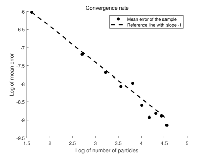
Figure 1: Euler Scheme with Particle Approximation

References

- [1] Alain Bensoussan. Stochastic control of partially observable systems. Cambridge University Press, Cambridge, 1992.
- [2] Alain Bensoussan, Xinwei Feng, and Jianhui Huang. Linear-quadratic-gaussian mean-field-game with partial observation and common noise. Mathematical Control & Related Fields, 11(1), 2021.
- [3] Rainer Buckdahn, Juan Li, and Jin Ma. A mean-field stochastic control problem with partial observations. The Annals of applied probability, 27(5):3201–3245, 2017.
- [4] Rainer Buckdahn, Juan Li, and Jin Ma. A general conditional mckean–vlasov stochastic differential equation. The Annals of Applied Probability, 33(3):2004–2023, 2023.
- [5] René Carmona, François Delarue, et al. Probabilistic theory of mean field games with applications I-II. Springer, 2018.
- [6] Michele Coghi and Franco Flandoli. Propagation of chaos for interacting particles subject to environmental noise. The Annals of applied probability, 26(3):1407–1442, 2016.
- [7] Dan Crisan, Jessica Gaines, and Terry Lyons. Convergence of a branching particle method to the solution of the zakai equation. SIAM Journal on Applied Mathematics, 58(5):1568–1590, 1998.
- [8] Dan Crisan, Thomas G. Kurtz, and Yoonjung Lee. Conditional distributions, exchangeable particle systems, and stochastic partial differential equations. Ann. Inst. Henri Poincaré Probab. Stat., 50(3):946–974, 2014.
- [9] Dan Crisan and Terry Lyons. A particle approximation of the solution of the kushner–stratonovitch equation. Probability Theory and Related Fields, 115:549–578, 1999.
- [10] Xavier Erny, Eva Löcherbach, and Dasha Loukianova. Conditional propagation of chaos for mean field systems of interacting neurons. Electronic Journal of Probability, 26:1–25, 2021.
- [11] Dena Firoozi and Peter E Caines. -nash equilibria for major–minor lqg mean field games with partial observations of all agents. IEEE Transactions on Automatic Control, 66(6):2778–2786, 2020.
- [12] William RP Hammersley, David Šiška, and Łukasz Szpruch. Weak existence and uniqueness for mckean–vlasov sdes with common noise. Annals of Probability, 49(2):527–555, 2021.
- [13] Joseph Horowitz and Rajeeva L Karandikar. Mean rates of convergence of empirical measures in the wasserstein metric. Journal of Computational and Applied Mathematics, 55(3):261–273, 1994.
- [14] Nobuyuki Ikeda and Shinzo Watanabe. Stochastic differential equations and diffusion processes. Elsevier, 2014.
- [15] Chaman Kumar, Neelima, Christoph Reisinger, and Wolfgang Stockinger. Well-posedness and tamed schemes for mckean–vlasov equations with common noise. The Annals of Applied Probability, 32(5):3283–3330, 2022.
- [16] Thomas G Kurtz and Jie Xiong. Particle representations for a class of nonlinear spdes. Stochastic Processes and their Applications, 83(1):103–126, 1999.
- [17] Thomas G Kurtz and Jie Xiong. Numerical solutions for a class of spdes with application to filtering. Stochastics in Finite and Infinite Dimensions: In Honor of Gopinath Kallianpur, pages 233–258, 2001.
- [18] Thomas G Kurtz and Jie Xiong. A stochastic evolution equation arising from the fluctuations of a class of interacting particle systems. Communications in Mathematical Sciences, 2(3):325–358, 2004.
- [19] Juan Li, Hao Liang, and Chao Mi. A stochastic maximum principle for partially observed general mean-field control problems with only weak solution. Stochastic Processes and their Applications, 165:397–439, 2023.
- [20] Min Li, Tianyang Nie, and Zhen Wu. Linear-quadratic large-population problem with partial information: Hamiltonian approach and riccati approach. SIAM Journal on Control and Optimization, 61(4):2114–2139, 2023.
- [21] Ruijing Li and Fengyun Fu. The maximum principle for partially observed optimal control problems of mean-field fbsdes. International Journal of Control, 92(10):2463–2472, 2019.
- [22] Yunzhang Li, Xiaolu Tan, and Shanjian Tang. Discrete-time approximation of stochastic optimal control with partial observation. SIAM Journal on Control and Optimization, 62(1):326–350, 2024.
- [23] Qi Lü and Xu Zhang. Mathematical control theory for stochastic partial differential equations. Springer, 2021.
- [24] Jin Ma, Rentao Sun, and Yonghui Zhou. Kyle–back equilibrium models and linear conditional mean-field sdes. SIAM Journal on Control and Optimization, 56(2):1154–1180, 2018.
- [25] E Pardoux. Equations of non-linear filtering; and application to stochastic control with partial observation. In Nonlinear Filtering and Stochastic Control: Proceedings of the 3rd 1981 Session of the Centro Internazionale Matematico Estivo (CIME), Held at Cortona, July 1–10, 1981, pages 208–248. Springer, 2006.
- [26] Nevroz Sen and Peter E Caines. Mean field games with partial observation. SIAM Journal on Control and Optimization, 57(3):2064–2091, 2019.
- [27] Shanjian Tang. The maximum principle for partially observed optimal control of stochastic differential equations. SIAM Journal on Control and optimization, 36(5):1596–1617, 1998.
- [28] Guangchen Wang and Zhen Wu. The maximum principles for stochastic recursive optimal control problems under partial information. IEEE Transactions on Automatic control, 54(6):1230–1242, 2009.
- [29] Nick P Whiteley. Stability properties of some particle filters. Annals of Applied Probability, 23(6):2500–2537, 2013.
- [30] Weian Zheng. Conditional propagation of chaos and a class of quasilinear pde’s. The Annals of Probability, pages 1389–1413, 1995.