Linear Numerical Schemes for a Q-Tensor System for Nematic Liquid Crystals

Abstract

In this work, we present three linear numerical schemes to model nematic liquid crystals using the Landau-de Gennes Q-tensor theory. The first scheme is based on using a truncation procedure of the energy, which allows for an unconditionally energy stable first order accurate decoupled scheme. The second scheme uses a modified second order accurate optimal dissipation algorithm, which gives a second order accurate coupled scheme. Finally, the third scheme uses a new idea to decouple the unknowns from the second scheme which allows us to obtain accurate dynamics while improving computational efficiency. We present several numerical experiments to offer a comparative study of the accuracy, efficiency and the ability of the numerical schemes to represent realistic dynamics.

1 Introduction

Liquid crystals (LCs) are important materials that are used in several technological applications [25]. The most common usage is in the omnipresent liquid crystal displays which uses the birefringence property of the material to create images on a screen [10]. However, LCs also respond to other external stimuli, e.g. magnetic, mechanical, chemical, which can be used to induce complex shape changes in the material used for applications in biomedical devices, robotics, optics, textiles, and sensors [11, 13, 28, 33, 34, 40].
Liquid crystals exhibit intermediary phases between solid and liquid. One such phase is the nematic phase which possess the microscopic orientational order of a crystalline solid, however, the molecules have no positional order but flow freely past each other and thus display macroscopic properties of a liquid. Models of LCs usually represent molecules as rods or disks and use some parameter to describe the orientation of the molecules. Popular models of LCs are the Oseen-Frank director theory [16, 31], the Ericksen-Leslie formulation [14, 15, 26, 27], and the hydrodynamic Beris-Edwards model [5].
In this work, we focus on the Landau-de Gennes Q-tensor theory [17, 30, 37] which can be seen as a subsystem of the Beris-Edwards model without hydrodynamic effects. In the Q-tensor model the orientation of the nematic is associated with a second-order tensor field which measures the local average deviation of the material from the isotropic state. This model has the advantage of being able to simulate complex defect dynamics due to its ability to describe more general defect geometries, and variable degrees of order [4].
Several analytic results exist concerning the well-posedness of the PDE associated to the Q-tensor problem coupled with the Navier-Stokes equations [1, 2, 12, 21, 32, 41]. The development of numerical schemes for this problem is relatively new, and faces certain challenges including: (1) the complex dynamics relating the physical properties of these materials cause the systems to be very large with several equations and unknowns; and (2) the equations are highly nonlinear with terms that couple the unknowns from different equations. Since the model involves a large system of coupled nonlinear PDEs we expect the discretization of this system to involve large and computationally expensive systems to solve.
Recently, we have seen new numerical methods proposed for modeling LC dynamics using the Q-tensor theory. For example, in [9] the authors present a first order accurate energy stable scheme for the 2D Q-tensor model with hydrodynamic effects. A stabilized convex splitting idea is used to develop a first order accurate decoupled energy stable scheme in [43]. In [42], a second order accurate scheme is presented for the hydrodynamic Q-tensor model using energy quadratization (IEQ) [19]. Error estimates for the IEQ approach has been recently presented to the Q-tensor model [20], and the Beris-Edwards model [39]. Another idea presented in [36] uses a scalar auxiliary variable (SAV) technique [18] to construct a second order accurate coupled scheme for a Q-tensor problem. Another recent and interesting paper explored numerical schemes for a hydrodynamic Q-tensor model in thin films [7]. In addition, work has been done on energy minimization techniques to compute equilibrium solutions for the Q-tensor problem such as [6, 35, 38].
In this paper, we propose three new efficient linear numerical schemes for simulating nematic liquid crystals using a Q-tensor model. The first scheme adapts an energy truncation procedure [8] which allows for an unconditionally energy stable first order accurate decoupled scheme. The second scheme uses a modified second order accurate optimal dissipation algorithm [22] which gives a second order accurate coupled scheme. Finally, the third scheme uses a technique to decouple the unknowns from the second scheme which allows us to recover accurate dynamics while improving computational efficiency.
The rest of the paper is organized as follows. In Section 2 we describe the Q-tensor model and some analytical results that are known about the problem. Next, we introduce the numerical schemes and their properties in Section 3. In Section 4 we provide computational results to justify the applicability and efficiency our numerical schemes. Finally, we state the conclusions of our work in Section 5 .

2 Landau-deGennes Q-Tensor Model

In this section we provide an overview of the Landau-de Gennes Q-Tensor model pertaining to the nematic phase of liquid crystals [17]. An alternative to the Oseen-Frank director theory [16], is to use the second order symmetric and traceless tensor Q representing the statistical second moment of the nematic system from the isotropic phase. In the isotropic phase $\textbf{Q}=\mathbf{0}$, and nonzero in the nematic phase. The eigenvalues of Q describe further phase transitions with the uniaxial phase corresponding to the case where Q has two equal eigenvalues, and otherwise the system is described as biaxial [30]. Let $\Omega\subset\mathbb{R}^{d}$, $d=2,3$, be a bounded domain with polyhedral boundary $\partial\Omega$. We will use the following tensor spaces

$$\begin{array}[]{rcl}\displaystyle\Lambda&:=&\{\textbf{Q}\in\mathbb{R}^{d\times d}:\textbf{Q}^{T}=\textbf{Q}\}\,,\\ \Lambda_{0}&:=&\{\textbf{Q}\in\mathbb{R}^{d\times d}:\textbf{Q}^{T}=\textbf{Q},\texttt{tr}(\textbf{Q})=0\}\,.\end{array}$$

Each $\textbf{Q}\in\Lambda$ is uniquely determined by six variables $\{q_{i}\}_{i=1}^{6}$ thus can be written as

$$\textbf{Q}\,=\,\begin{pmatrix}Q_{11}&Q_{12}&Q_{13}\\ Q_{21}&Q_{22}&Q_{23}\\ Q_{31}&Q_{32}&Q_{33}\end{pmatrix},$$

and each $\textbf{Q}\in\Lambda_{0}$ can be uniquely determined by five unknowns (with $Q_{33}=-(Q_{11}+Q_{22})$). Here we use spatial coordinates $\mathbf{x}\in\mathbb{R}^{d}$. It is useful to write Q in its eigenframe

$$\textbf{Q}=s_{1}(\mathbf{v}_{1}\otimes\mathbf{v}_{1})+s_{2}(\mathbf{v}_{2}\otimes\mathbf{v}_{2})-\frac{1}{3}(s_{1}+s_{2})\mathbf{I}\,,$$

where $\mathbf{I}$ is the identity matrix, $\mathbf{v}_{i}$, are the orthonormal eigenvectors of Q, and $s_{i}$ are linear combinations of the corresponding eigenvalues $\lambda_{i}$ given by

$$\lambda_{1}\,=\,\frac{1}{3}(2s_{1}-s_{2})\,,\quad\lambda_{2}\,=\,-\frac{1}{3}(s_{1}+s_{2})\,,\quad\lambda_{3}\,=\,\frac{1}{3}(2s_{2}-s_{1})\,.$$

Since $\texttt{tr}(\textbf{Q})=0$, we have that $\sum_{i}\lambda_{i}=0$. Furthermore, the eigenvalues are restricted to the range $-\frac{1}{3}\leq\lambda_{i}\leq\frac{2}{3}$ [37].

The Landau-deGennes free energy function is defined as:

$$E(\textbf{Q})\,:=\,\int_{\Omega}\left(\mathcal{W}(\textbf{Q},\nabla\textbf{Q})+\frac{1}{\varepsilon}\Psi(\textbf{Q})\right)d\mathbf{x}\,,$$ (1)

with $\mathcal{W}(\textbf{Q},\nabla\textbf{Q})$ being the elastic energy density and $\Psi(\textbf{Q})$ representing the thermotropic energy density, respectively. Moreover, $\varepsilon>0$ is a dimensionless parameter balancing the energetic contributions of the elastic and thermotropic energies.

2.1 Elastic Energy Density

The elastic energy is given by

$$\mathcal{W}(\textbf{Q},\nabla\textbf{Q})\,:=\,\frac{1}{2}\left(L_{1}\left|\nabla\textbf{Q}\right|^{2}+L_{2}\left|\nabla\cdot\textbf{Q}\right|^{2}+L_{3}\left(\nabla\textbf{Q}\right)^{T}\,\vdots\,\nabla\textbf{Q}+L_{4}\nabla\textbf{Q}\,\vdots\,(\bm{\epsilon}\cdot\textbf{Q})+L_{5}\nabla\textbf{Q}\,\vdots\,(\textbf{Q}\cdot\nabla)\textbf{Q})\right),$$ (2)

where $L_{i}$, $i=1,\dots,5$ are the elastic material parameters and $\vdots$ represents the scalar product between third order tensors. Then, using the convention of summation over repeated indices, the elastic energy terms can be written as

$$\left|\nabla\textbf{Q}\right|^{2}:=\frac{\partial}{\partial x_{k}}Q_{ij}\frac{\partial}{\partial x_{k}}Q_{ij}\,,\quad\quad\left|\nabla\cdot\textbf{Q}\right|^{2}:=\frac{\partial Q_{ij}}{\partial x_{j}}\frac{\partial Q_{ik}}{\partial x_{k}}\,,\quad\quad\left(\nabla\textbf{Q}\right)^{T}\,\vdots\,\nabla\textbf{Q}:=\frac{\partial Q_{ik}}{\partial x_{j}}\frac{\partial Q_{ij}}{\partial x_{k}}\,,$$

$$\nabla\textbf{Q}\,\vdots\,(\bm{\epsilon}\cdot\textbf{Q}):=\bm{\epsilon}_{ijk}Q_{lj}\frac{\partial Q_{ij}}{\partial x_{k}}\,,\quad\quad\nabla\textbf{Q}\,\vdots\,(\textbf{Q}\cdot\nabla)\textbf{Q}):=Q_{lk}\frac{\partial Q_{ij}}{\partial x_{l}}\frac{\partial Q_{ij}}{\partial x_{k}}\,,$$

where $\bm{\epsilon}$ is the Levi-Civita permutation symbol. The five elastic constants $L_{i}$ can be related to the Oseen-Frank model constants $K_{i}$, for $i=1,\dots,4$, and chirality $q_{0}$ [30]. In this work we consider the one constant Landau-deGennes model with $L_{i}=0$ for $i=2,\dots,5$.

2.2 Landau-deGennes Potential Function

The second term of the energy corresponds to the thermotropic contribution. The Landau-de Gennes potential functional $\Psi(\textbf{Q})$ describes the various states of the nematic system, i.e. uniaxial nematic, biaxial nematic, or isotropic liquid. The most general form of this function is written as

$$\Psi(\textbf{Q})\,=\,\frac{A}{2}\texttt{tr}(\textbf{Q}^{2})-\frac{B}{3}\texttt{tr}(\textbf{Q}^{3})+\frac{C}{4}\texttt{tr}(\textbf{Q}^{2})^{2}\,.$$ (3)

The parameters $A,B$, and $C$ depend on the material being studied. We consider $B,C>0$ and independent of temperature $\theta$, while $A(\theta)=\widehat{\gamma}(\theta-\theta^{*})$, with $\widehat{\gamma}>0$ and $\theta^{*}$ being the isotropic-nematic phase transition temperature [29, 30]. Here, $\texttt{tr}(\textbf{Q}):=Q_{ii}$, and the higher order terms can be written as

$$\texttt{tr}(\textbf{Q}^{2})\,:=\,Q_{ij}Q_{ij}\,,\quad\texttt{tr}(\textbf{Q}^{3})\,:=\,Q_{ij}Q_{jk}Q_{ki}\,.$$

It is known that when $B\neq 0$ the symmetric and traceless tensors which minimize Equation 3 will have two equal eigenvalues, i.e. the uniaxial state [37]. Minimizing the total free energy involves a balance of competing energy terms from the elastic and thermotropic components. In this way, it is important to choose parameters $L_{i}$, and $A,B,C$ properly to ensure the energy functional $E(\textbf{Q})$ is bounded from below [29].

2.3 System Dynamics

The dynamics of the system are given by using an $L^{2}$-gradient flow

$$\textbf{Q}_{t}+\gamma\frac{\delta E(\textbf{Q})}{\delta\textbf{Q}}\,=\,\textbf{0}\,,$$

with $\gamma$ being a relaxation parameter and the variational derivative of the energy given by

$$\frac{\delta E(\textbf{Q})}{\delta\textbf{Q}}\,=\,-\Delta\textbf{Q}+\frac{1}{\varepsilon}\nabla\Psi(\textbf{Q})\,,$$

which results in the following formulation of the problem: Given $\textbf{Q}_{0}(\mathbf{x}):\Omega\rightarrow\Lambda_{0}$, find $\textbf{Q}(\mathbf{x},t):\Omega\times(0,T)\rightarrow\Lambda_{0}$ such that

$$\left\{\begin{array}[]{rclr}\displaystyle\textbf{Q}_{t}+\gamma\left(-\Delta\textbf{Q}+\frac{1}{\varepsilon}\bm{\psi}(\textbf{Q})\right)&=&\mathbf{0}&\quad\mbox{ for }(\mathbf{x},t)\in\Omega\times(0,T)\,,\\ \partial_{\mathbf{n}}\textbf{Q}&=&\mathbf{0}&\quad\mbox{ for }(\mathbf{x},t)\in\partial\Omega\times(0,T)\,,\\ \textbf{Q}(\mathbf{x},0)&=&\textbf{Q}_{0}(\mathbf{x})&\quad\mbox{ for }\mathbf{x}\in\Omega\,,\end{array}\right.$$ (4)

where $\mathbf{n}$ denotes the unit outward normal vector on $\partial\Omega$, $\partial_{\mathbf{n}}\textbf{Q}=\nabla\textbf{Q}\cdot\mathbf{n}$, and $T>0$ is the final time. Here, the gradient of $\Psi$ with respect to Q is a second order tensor, $\bm{\psi}$, given by

$$\bm{\psi}(\textbf{Q}):=\nabla\Psi(\textbf{Q})=A\textbf{Q}-B\textbf{Q}^{2}+C\texttt{tr}(\textbf{Q}^{2})\textbf{Q}\,.$$ (5)

Additionally, we write the second derivative of $\Psi$, which is a fourth order tensor, $\nabla\bm{\psi}(\textbf{Q})$, as

$$\left[\nabla\bm{\psi}(\textbf{Q})\right]_{ijkl}=A\delta_{ik}\delta_{jl}-B\left(Q_{lj}\delta_{ik}+Q_{ik}\delta_{jl}\right)+C\left(\texttt{tr}(\textbf{Q}^{2})\delta_{ik}\delta_{jl}+2Q_{ij}Q_{kl}\right)\,,$$ (6)

with $\delta_{ij}$ denoting the Kronecker delta function.

Remark 1.

See appendix for details on the computations in (6).

2.4 Traceless Formulation

Following the ideas in [21], we provide a reformulation of the Landau-de Gennes model to facilitate the development of numerical schemes. First, to maintain the traceless condition on Q we replace the variational derivative with the following expression:

$$\textbf{Q}_{t}+\gamma\left(\frac{\delta E(\textbf{Q})}{\delta\textbf{Q}}-\frac{1}{3}\texttt{tr}\left(\frac{\delta E(\textbf{Q})}{\delta\textbf{Q}}\right)\right)\,=\,\mathbf{0}\,.$$

Hence, the problem reads:

$$\left\{\begin{array}[]{rclr}\displaystyle\textbf{Q}_{t}+\gamma\left[-\Delta\textbf{Q}+\frac{1}{\varepsilon}\left(A\textbf{Q}-B\left(\textbf{Q}^{2}\right)+C\texttt{tr}(\textbf{Q}^{2})\textbf{Q}\right)+\frac{1}{\varepsilon}\bm{p}(\textbf{Q})\right]&=&\mathbf{0}&\quad\mbox{ for }(\mathbf{x},t)\in\Omega\times(0,T)\,,\\ \partial_{\mathbf{n}}\textbf{Q}&=&\mathbf{0}&\quad\mbox{ for }(\mathbf{x},t)\in\partial\Omega\times(0,T)\,,\\ \textbf{Q}(\mathbf{x},0)&=&\textbf{Q}_{0}(\mathbf{x})&\quad\mbox{ for }\mathbf{x}\in\Omega\,,\end{array}\right.$$ (7)

where the function $\bm{p}(\textbf{Q})$ represents the non-zero trace part of the problem:

$$\bm{p}(\textbf{Q})=-\frac{B}{3}\texttt{tr}(\textbf{Q}^{2})\mathbf{I}\,.$$

Remark 2.

Another possible way to enforce the traceless condition on Q is to derive the dynamics by taking the variational derivative with respect to a symmetric and traceless tensor which will intrinsically impose the condition [37, 38].

Now we summarize various results presented in [21] about the problem (4) and the modified problem (7), both coupled with hydrodynamics effects.

Theorem 1 (Well-Posedness).

Let $\textbf{Q}_{0}\in H^{1}(\Omega)$. Then there exists a weak solution Q of the problem (7) such that,

$$\textbf{Q}\in L^{\infty}(0,\infty;H^{1}(\Omega))\cap L^{2}(0,T;H^{2}(\Omega)),\quad\forall T>0\,.$$

Furthermore, if Q is a solution to (7) in $(0,T)$ for some fixed $T>0$, and

$$\Delta\textbf{Q}\in L^{\frac{2s}{2s-3}}(0,T;L^{s}(\Omega))\mbox{ for some }2\leq s\leq 3\,,$$

then the solution is unique.

Lemma 1 (Traceless Property).

If $\texttt{tr}(\textbf{Q}_{0})=0$, then $\texttt{tr}(\textbf{Q})=0$ for all $t>0$.

Additionally, this continuous problem possesses the following maximum principle on the norm of Q. Here, we use the Frobenius norm $|\textbf{Q}|=\sqrt{\textbf{Q}:\textbf{Q}}$ where $\textbf{Q}:\textbf{Q}=Q_{ij}Q_{ij}$.

Lemma 2 (Maximum Principle).

Let $\alpha>0$ satisfy

$$\alpha^{2}\geq\frac{B^{2}}{C^{2}}-\frac{2A}{C}\,,$$ (8)

where $A,B$, and $C$ are the coefficients in the potential function $\Psi(\textbf{Q})$. Let $\textbf{Q}_{0}\in H^{1}(\Omega)$ with $|\textbf{Q}_{0}|\leq\alpha$ a.e. in $\Omega$. If $\textbf{Q}\in L^{\infty}(0,T;H^{1}(\Omega))\cap L^{2}(0,T;H^{2}(\Omega))$ is any point-wise solution for the problem (7) in $(0,T)\times\Omega$ then

$$|\textbf{Q}(\mathbf{x},t)|\leq\alpha\mbox{ a.e. }(\mathbf{x},t)\in(0,T)\times\Omega\,.$$

Lemma 3 (Energy Law).

The problem satisfies the following dissipative energy law

$$\frac{d}{dt}E(\textbf{Q})+\frac{1}{\gamma}\|\textbf{Q}_{t}\|^{2}_{L^{2}}=0\,.$$ (9)

3 Numerical Schemes

The main challenge for developing numerical schemes to approximate solutions to (4) is the nonlinearity of the unknowns in the potential function $\Psi(\textbf{Q})$. There are two main objectives we pursue to design numerical schemes. The first goal is to design schemes that obey a dissipative energy law for the discrete problem similar to the one associated with the continuous problem (equation (9)), so that we can guarantee decreasing energy in time. The second will be to stay as close as possible to the energy law at the discrete level so that we can recover the dynamics of the system more accurately.
Within this study, we intend to introduce a linear, unconditionally energy-stable Finite Element numerical method for the simulation of nematic liquid crystals. Subsequently, we explore a series of numerical techniques that enhance computational efficiency but come at the expense of compromising the structure-preserving attributes of the initial method. Notably, substantial reductions in computational cost can be achieved by reconfiguring the problem formulation to decouple the six unknown variables. This modification allows us to tackle multiple smaller problems sequentially, as opposed to dealing with a single, large linear system. Indeed, we will demonstrate the feasibility of implementing this concept for three-dimensional simulations with a relatively fine spatial mesh.

3.1 A Finite Element Space-Discrete Scheme

In this section we develop numerical schemes for the weak formulation of the modified problem (7). The $L^{2}$ inner product is denoted by $(\cdot,\cdot)$. We consider a Finite Element method for space discretization as follows. Let $\bm{K}_{h}\subset H^{1}(\Omega)$ be a conformed finite element space associated to a regular and quasi-uniform triangulation $\mathcal{T}_{h}$ of the domain $\Omega$ whose polyhedric boundary is denoted by $\partial\Omega$. For the sake of notation, we skip the use of the subscript $h$ to denote functions that are discrete in space. Then the Finite Element approximation of (7) is: Find $\textbf{Q}(\mathbf{x},t)\in\bm{K}_{h}$ such that

$$\textbf{Q}(\mathbf{x},0)=P_{\bm{K}_{h}}\textbf{Q}_{0}\,,$$

where $P_{\bm{K}_{h}}$ denotes the projection operator into the space $\bm{K}_{h}$, and

$$\left(\textbf{Q}_{t},\overline{\textbf{Q}}\right)+\gamma\left[\left(\nabla\textbf{Q},\nabla\overline{\textbf{Q}}\right)+\frac{1}{\varepsilon}\left(\bm{\psi}(\textbf{Q}),\overline{\textbf{Q}}\right)+\frac{1}{\varepsilon}\left(\bm{p}(\textbf{Q}),\overline{\textbf{Q}}\right)\right]\,=\,0\,,$$

for any $\overline{\textbf{Q}}\in\bm{K}_{h}$.

3.2 Fully Discrete Schemes

We consider a Finite Difference method in time using a regular partition of the interval $[0,T]$ into steps of length $\Delta t>0$. We denote $t^{n}:=n\Delta t$, $\textbf{Q}^{n}$ represents the approximation of $\textbf{Q}(\mathbf{x},t^{n})$ with $\textbf{Q}^{0}=P_{\bm{K}_{h}}\textbf{Q}_{0}$,

$$\delta_{t}u^{n+1}\,:=\,\frac{u^{n+1}-u^{n}}{\Delta t}\quad\quad\mbox{ and }\quad\quad u^{n+\frac{1}{2}}\,:=\,\frac{u^{n+1}+u^{n}}{2}\,.$$

Recall that the nonlinearity of the model exists in the potential function $\bm{\psi}(\textbf{Q})$. The main contribution of our work relies in proposing numerical schemes with linear approximations to $\bm{\psi}(\textbf{Q})$ for which we write $\bm{\psi}^{\Delta t}(\textbf{Q}^{n+1},\textbf{Q}^{n})$.
We propose the following generic numerical scheme.

• Initialization: Let $\textbf{Q}^{0}\in\bm{K}_{h}$ satisfying $\textbf{Q}^{0}\in\Lambda_{0}$, and $|\textbf{Q}^{0}|\leq\alpha$ a.e. in $\Omega$.
  

• Step $n+1$: given $\textbf{Q}^{n}\in\bm{K}_{h}$, find $\textbf{Q}^{n+1}\in\bm{K}_{h}$ such that

  $$\begin{array}[]{rcl}\displaystyle\left(\delta_{t}\textbf{Q}^{n+1},\overline{\textbf{Q}}\right)+\gamma\left[\left(\nabla\textbf{Q}^{n+\frac{1}{2}},\nabla\overline{\textbf{Q}}\right)+\frac{1}{\varepsilon}\left(\bm{\psi}^{\Delta t}(\textbf{Q}^{n+1},\textbf{Q}^{n}),\overline{\textbf{Q}}\right)+\frac{1}{\varepsilon}\left(\bm{p}(\textbf{Q}^{n+1},\textbf{Q}^{n}),\overline{\textbf{Q}}\right)\right]&=&0\,,\end{array}$$ (10)

  for all $\overline{\textbf{Q}}\in\bm{K}_{h}$.

Lemma 4 (Discrete Energy Law).

The generic numerical scheme (10) satisfies a discrete version of the energy law (9):

$$\delta_{t}E(\textbf{Q}^{n+1})+\frac{1}{\gamma}\frac{1}{(\Delta t)^{2}}||\textbf{Q}^{n+1}-\textbf{Q}^{n}||_{L^{2}}^{2}+\mathbf{ND}\left(\textbf{Q}^{n+1},\textbf{Q}^{n}\right)=0\,,$$ (11)

where $\mathbf{ND}\left(\textbf{Q}^{n+1},\textbf{Q}^{n}\right)$ denotes the numerical dissipation

$$\begin{array}[]{rcl}\mathbf{ND}\left(\textbf{Q}^{n+1},\textbf{Q}^{n}\right)&:=&\displaystyle\frac{1}{\varepsilon\Delta t}\int_{\Omega}\left(\bm{\psi}^{\Delta t}(\textbf{Q}^{n+1},\textbf{Q}^{n}):(\textbf{Q}^{n+1}-\textbf{Q}^{n})\right)-\left(\Psi(\textbf{Q}^{n+1})-\Psi(\textbf{Q}^{n})\right)d\mathbf{x}\\ \vskip 6.0pt plus 2.0pt minus 2.0pt\cr&&\displaystyle+\frac{1}{\varepsilon\Delta t}\int_{\Omega}\bm{p}(\textbf{Q}^{n+1},\textbf{Q}^{n})\left(\texttt{tr}(\textbf{Q}^{n+1})-\texttt{tr}(\textbf{Q}^{n})\right).\end{array}$$ (12)

Proof.

Take $\overline{\textbf{Q}}=\frac{1}{\gamma}\delta_{t}\textbf{Q}^{n+1}$ in (10). We obtain

$$\begin{array}[]{rcl}\displaystyle\frac{1}{\Delta t}\left(\frac{1}{2}||\nabla\textbf{Q}^{n+1}||_{L^{2}}-\frac{1}{2}||\nabla\textbf{Q}^{n}||_{L^{2}}\right)+\frac{1}{\gamma}\frac{1}{(\Delta t)^{2}}||\textbf{Q}^{n+1}-\textbf{Q}^{n}||_{L^{2}}^{2}&&\\ \vskip 6.0pt plus 2.0pt minus 2.0pt\cr\displaystyle+\frac{1}{\varepsilon\Delta t}\left(\bm{\psi}^{\Delta t}(\textbf{Q}^{n+1},\textbf{Q}^{n}),(\textbf{Q}^{n+1}-\textbf{Q}^{n})\right)+\frac{1}{\varepsilon\Delta t}\left(\bm{p}(\textbf{Q}^{n+1},\textbf{Q}^{n}),(\textbf{Q}^{n+1}-\textbf{Q}^{n})\right)&=&0\,.\end{array}$$

Therefore, by adding and subtracting $\varepsilon^{-1}\left(\Psi(\textbf{Q}^{n+1})-\Psi(\textbf{Q}^{n})\right)$,

$$\begin{array}[]{rcl}\displaystyle\frac{E(\textbf{Q}^{n+1})-E(\textbf{Q}^{n})}{\Delta t}+\frac{1}{\gamma}\frac{1}{(\Delta t)^{2}}||\textbf{Q}^{n+1}-\textbf{Q}^{n}||_{L^{2}}^{2}&&\\ \vskip 6.0pt plus 2.0pt minus 2.0pt\cr\displaystyle+\frac{1}{\varepsilon\Delta t}\int_{\Omega}\left(\bm{\psi}^{\Delta t}(\textbf{Q}^{n+1},\textbf{Q}^{n}):(\textbf{Q}^{n+1}-\textbf{Q}^{n})\right)-\left(\Psi(\textbf{Q}^{n+1})-\Psi(\textbf{Q})\right)d\mathbf{x}&&\\ \vskip 6.0pt plus 2.0pt minus 2.0pt\cr\displaystyle+\frac{1}{\varepsilon\Delta t}\int_{\Omega}\bm{p}(\textbf{Q}^{n+1},\textbf{Q}^{n})\left(\texttt{tr}(\textbf{Q}^{n+1})-\texttt{tr}(\textbf{Q}^{n})\right)d\mathbf{x}&=&0\,.\end{array}$$

∎

Definition 1.

A numerical scheme is energy stable if

$$\frac{E(\textbf{Q}^{n+1})-E(\textbf{Q}^{n})}{\Delta t}+\frac{1}{\gamma}||\delta_{t}\textbf{Q}^{n+1}||_{L^{2}}^{2}\,\leq\,0\quad\quad\forall\,n\geq 0\,.$$ (13)

In particular, energy stability implies the decreasing energy property $E(\textbf{Q}^{n+1})\leq E(\textbf{Q}^{n})$ for all $n\geq 1$. Moreover, if the scheme can be shown to satisfy (13) for any choice of $\Delta t>0$, then the scheme is called unconditionally energy stable.

Remark 3.

From (11), the numerical scheme (10) is energy stable if

$$\mathbf{ND}(\textbf{Q}^{n+1},\textbf{Q}^{n})\geq 0\,.$$ (14)

The main contribution of this paper is to present different choices of $\bm{\psi}^{\Delta t}(\textbf{Q}^{n+1},\textbf{Q}^{n})$ so that we may control the sign and/or size of the numerical dissipation (12). The key point of our approach is to derive numerical schemes whose solutions are as close to the solution of the original problem as possible. In fact, one of the goals of this work is to emphasize that even schemes that are not unconditionally energy stable can be reliable if the size of the numerical dissipation is small.

In the next sections we develop three choices for $\bm{\psi}^{\Delta t}(\textbf{Q}^{n+1},\textbf{Q}^{n})$ along with their properties.

3.2.1 First Order Unconditionally Energy Stable Decoupled Scheme (UES1D)

Here, we present a linear, first order accurate in time, unconditionally energy stable numerical scheme. Let $\alpha>0$ satisfy (8) from the maximum principle on $|\textbf{Q}|$. Consider splitting $\Psi(\textbf{Q})$ into three terms:

$$\begin{array}[]{rcl}\displaystyle\Psi(\textbf{Q})&=&\Psi_{1}(\textbf{Q})+\Psi_{2}(\textbf{Q})+\Psi_{3}(\textbf{Q})\,,\end{array}$$ (15)

such that

$$\begin{array}[]{rcl}\displaystyle\Psi_{1}(\textbf{Q})&=&\displaystyle\frac{C}{4}\left(\texttt{tr}(\textbf{Q}^{2})-\alpha^{2}\right)^{2}\,,\\ \vskip 6.0pt plus 2.0pt minus 2.0pt\cr\displaystyle\Psi_{2}(\textbf{Q})&=&\displaystyle\left(\frac{A}{2}+\frac{C\alpha^{2}}{2}\right)\texttt{tr}(\textbf{Q}^{2})-\frac{C}{4}\alpha^{4}\,,\\ \vskip 6.0pt plus 2.0pt minus 2.0pt\cr\displaystyle\Psi_{3}(\textbf{Q})&=&\displaystyle-\frac{B}{3}\texttt{tr}(\textbf{Q}^{3})\,.\end{array}$$ (16)

The first derivative is given by

$$\begin{array}[]{rcl}\bm{\psi}(\textbf{Q})&=&\displaystyle\bm{\psi}_{1}(\textbf{Q})+\bm{\psi}_{2}(\textbf{Q})+\bm{\psi}_{3}(\textbf{Q})\,,\end{array}$$ (17)

with

$$\begin{array}[]{rcl}\vskip 6.0pt plus 2.0pt minus 2.0pt\cr\bm{\psi}_{1}(\textbf{Q})&=&\displaystyle C\left(\texttt{tr}(\textbf{Q}^{2})-\alpha^{2}\right)\textbf{Q}\,,\\ \vskip 6.0pt plus 2.0pt minus 2.0pt\cr\vskip 6.0pt plus 2.0pt minus 2.0pt\cr\bm{\psi}_{2}(\textbf{Q})&=&\displaystyle\left(A+C\alpha^{2}\right)\textbf{Q}\,,\\ \vskip 6.0pt plus 2.0pt minus 2.0pt\cr\bm{\psi}_{3}(\textbf{Q})&=&\displaystyle-B\textbf{Q}^{2}\,.\end{array}$$ (18)

We will use different ideas to approximate each of the terms in $\bm{\psi}(\textbf{Q})$. First, since $\bm{\psi}_{2}(\textbf{Q})$ is linear in Q, in all the numerical schemes moving forward we will use the Crank-Nicolson approximation

$$\bm{\psi}_{2}^{\Delta t}(\textbf{Q})\,=\,\bm{\psi}_{2}\left(\textbf{Q}^{n+\frac{1}{2}}\right)\,=\,\left(A+C\alpha^{2}\right)\frac{\textbf{Q}^{n+1}+\textbf{Q}^{n}}{2}\,.$$ (19)

Next, by using the symmetry of $\Psi_{1}$ we consider a $\mathcal{C}^{2}$ truncation as follows:

$$\widehat{\Psi}_{1}(\textbf{Q})\,=\,\left\{\begin{array}[]{ll}\displaystyle\frac{C}{4}\left(\texttt{tr}(\textbf{Q}^{2})-\alpha^{2}\right)^{2}&\mbox{ if }|\textbf{Q}|\leq\alpha\,,\\ \vskip 6.0pt plus 2.0pt minus 2.0pt\cr C\alpha^{2}\left(|\textbf{Q}|-\alpha\right)^{2}&\mbox{ if }|\textbf{Q}|>\alpha\,.\\ \end{array}\right.$$ (20)

Note that $\texttt{tr}(\textbf{Q}^{2})=|\textbf{Q}|^{2}$ so $\widehat{\Psi}_{1}$ is continuous. Furthermore, the first derivative

$$\bm{\widehat{\psi}}_{1}(\textbf{Q})\,=\,\left\{\begin{array}[]{ll}\displaystyle C\left(\texttt{tr}(\textbf{Q}^{2})-\alpha^{2}\right)\textbf{Q}&\mbox{ if }|\textbf{Q}|\leq\alpha\,,\\ \vskip 6.0pt plus 2.0pt minus 2.0pt\cr 2C\alpha^{2}\left(|\textbf{Q}|-\alpha\right)\frac{\textbf{Q}}{|\textbf{Q}|}&\mbox{ if }|\textbf{Q}|>\alpha\,,\\ \end{array}\right.$$ (21)

and second derivative

$$\left[\nabla\bm{\widehat{\psi}}_{1}(\textbf{Q})\right]_{ijkl}\,=\,\left\{\begin{array}[]{ll}\displaystyle 2CQ_{ij}Q_{kl}+C(\texttt{tr}(\textbf{Q}^{2})-\alpha^{2})\delta_{ik}\delta_{jl}&\mbox{ if }|\textbf{Q}|\leq\alpha\,,\\ \vskip 6.0pt plus 2.0pt minus 2.0pt\cr 2C\alpha^{2}\left(\alpha\frac{q_{j}q_{l}}{|\textbf{Q}|^{3}}+\frac{|\textbf{Q}|-\alpha}{|\textbf{Q}|}\delta_{ik}\delta_{jl}\right)&\mbox{ if }|\textbf{Q}|>\alpha\,,\\ \end{array}\right.$$ (22)

are both continuous. Moreover, we have the following bounds on $\nabla\bm{\widehat{\psi}}_{1}(\textbf{Q})$

$$\left|\left|\left[\nabla\bm{\widehat{\psi}}_{1}(\textbf{Q})\right]_{ijkl}\right|\right|_{L^{\infty}}\,\leq\,2C\alpha^{2}(1+\delta_{ik}\delta_{jl})\quad\mbox{ and }\quad\left|\left|\nabla\bm{\widehat{\psi}}_{1}(\textbf{Q})\right|\right|_{F}\,\leq\,12\sqrt{3}C\alpha^{2}\,,$$ (23)

where the fourth order tensor Frobenius norm is $||\bm{A}||_{F}:=\sqrt{A_{ijkl}A_{ijkl}}$.

Finally, we would like to develop a $\mathcal{C}^{2}$ truncation for $\Psi_{3}$ but it lacks symmetry as in $\Psi_{1}$. Thus we follow the ideas presented in [38] and consider the following construction which smoothly transitions $\Psi_{3}$ into a function with bounded second derivative. Let $\rho:[0,\infty)\rightarrow\mathbb{R}$ be the following monotone function

$$\rho(r)\,:=\,\left\{\begin{array}[]{ll}\displaystyle 1&\mbox{ if }r\leq\sqrt{\alpha_{1}}\,,\\ \vskip 6.0pt plus 2.0pt minus 2.0pt\cr\displaystyle\left(2\frac{r-\alpha_{1}}{\alpha_{2}-\alpha_{1}}+1\right)\left(1-\frac{r-\alpha_{1}}{\alpha_{2}-\alpha_{1}}\right)^{2}&\mbox{ if }\sqrt{\alpha_{1}}<r<\sqrt{\alpha_{2}}\,,\\ \vskip 6.0pt plus 2.0pt minus 2.0pt\cr 0&\mbox{ if }\sqrt{\alpha_{2}}\leq r\,.\end{array}\right.$$ (24)

Here $\alpha<\alpha_{1}<\alpha_{2}$ are fixed constants where $\alpha$ is the value from the maximum principle (8). Then we modify $\Psi_{3}$ as follows

$$\widehat{\Psi}_{3}(\textbf{Q})=-\frac{B}{3}\texttt{tr}\textbf{Q}^{3}\rho(\texttt{tr}(\textbf{Q}^{2}))+\texttt{tr}(\textbf{Q}^{2})\left[1-\rho(\texttt{tr}(\textbf{Q}^{2}))\right]\,.$$ (25)

In this way, we do not change the function in the region $|\textbf{Q}|\leq\alpha$, and when $|\textbf{Q}|>\alpha$ we smoothly transition to a function of quadratic growth so that the Hessian tensor is bounded. There exist computable constants $s_{3,\infty}$, and $s_{3,F}$ (see appendix) such that

$$\left|\left|\left[\nabla\bm{\widehat{\psi}}_{3}(\textbf{Q})\right]_{ijkl}\right|\right|_{L^{\infty}}\,\leq\,s_{3,\infty}\quad\mbox{ and }\quad\left|\left|\nabla\bm{\widehat{\psi}}_{3}(\textbf{Q})\right|\right|_{F}\,\leq\,s_{3,F}.$$ (26)

Using these ideas, we write the truncated potential function $\widehat{\Psi}(\textbf{Q})$ as

$$\widehat{\Psi}(\textbf{Q})\,=\,\widehat{\Psi}_{1}(\textbf{Q})+\Psi_{2}(\textbf{Q})+\widehat{\Psi}_{3}(\textbf{Q})\,.$$ (27)

Then the modified energy $\widehat{E}(\textbf{Q})$ is

$$\widehat{E}(\textbf{Q})\,=\,\int_{\Omega}\left(\frac{1}{2}|\nabla\textbf{Q}|^{2}+\frac{1}{\varepsilon}\widehat{\Psi}(\textbf{Q})\right)d\mathbf{x}\,.$$ (28)

We write $\bm{\psi}^{\Delta t}$ as follows

$$\begin{array}[]{rcl}\bm{\psi}^{\Delta t}(\textbf{Q}^{n+1},\textbf{Q}^{n})&=&\displaystyle\bm{\psi}_{1}^{\Delta t}(\textbf{Q}^{n+1},\textbf{Q}^{n})+\bm{\psi}_{2}^{\Delta t}(\textbf{Q}^{n+1},\textbf{Q}^{n})+\bm{\psi}_{3}^{\Delta t}(\textbf{Q}^{n+1},\textbf{Q}^{n})\,,\end{array}$$ (29)

with

$$\begin{array}[]{rcl}\displaystyle\bm{\psi}_{1}^{\Delta t}(\textbf{Q}^{n+1},\textbf{Q}^{n})&=&\displaystyle\bm{\widehat{\psi}}_{1}(\textbf{Q}^{n})+\frac{1}{2}S_{1}\left(\textbf{Q}^{n+1}-\textbf{Q}^{n}\right)\,,\\ \vskip 6.0pt plus 2.0pt minus 2.0pt\cr\displaystyle\bm{\psi}_{2}^{\Delta t}(\textbf{Q}^{n+1},\textbf{Q}^{n})&=&\displaystyle\bm{\psi}_{2}\left(\textbf{Q}^{n+\frac{1}{2}}\right)\,,\\ \vskip 6.0pt plus 2.0pt minus 2.0pt\cr\displaystyle\bm{\psi}_{3}^{\Delta t}(\textbf{Q}^{n+1},\textbf{Q}^{n})&=&\displaystyle\bm{\widehat{\psi}}_{3}(\textbf{Q}^{n})+\frac{1}{2}S_{3}\left(\textbf{Q}^{n+1}-\textbf{Q}^{n}\right)\,.\end{array}$$ (30)

Then the scheme can be written as follows:

$$\left(\delta_{t}\textbf{Q}^{n+1},\overline{\textbf{Q}}\right)+\gamma\left[\left(\nabla\textbf{Q}^{n+\frac{1}{2}},\nabla\overline{\textbf{Q}}\right)+\frac{1}{\varepsilon}\left(\bm{\psi}^{\Delta t}(\textbf{Q}^{n+1},\textbf{Q}^{n}),\overline{\textbf{Q}}\right)+\frac{1}{\varepsilon}\left(\bm{p}(\textbf{Q}^{n}),\overline{\textbf{Q}}\right)\right]\,=\,0\,,$$ (31)

for all $\overline{\textbf{Q}}\in\bm{K}_{h}$. Here, we choose the trace part of the problem to be approximated as

$$p(\textbf{Q}^{n})=-\frac{1}{3}\texttt{tr}\left(\bm{\widehat{\psi}}_{3}(\textbf{Q}^{n})\right)\mathbf{I}=\frac{B}{3}\texttt{tr}\left((\textbf{Q}^{n})^{2}\right)\mathbf{I}\,.$$ (32)

Lemma 5.

Scheme UES1D satisfies a discrete version of 1. For any positive constants $S_{1}$, and $S_{3}$, if $\texttt{tr}(\textbf{Q}^{n})=0$, then $\texttt{tr}(\textbf{Q}^{n+1})=0$.

Proof.

In (31) let $\overline{\textbf{Q}}=\frac{1}{\gamma}\texttt{tr}(\textbf{Q}^{n+1})\mathbf{I}$. Then we obtain

$$\begin{array}[]{rcl}\displaystyle\frac{1}{\gamma}\frac{1}{\Delta t}\left(\texttt{tr}(\textbf{Q}^{n+1}),\texttt{tr}(\textbf{Q}^{n+1})\right)-\frac{1}{\gamma}\frac{1}{\Delta t}\left(\texttt{tr}(\textbf{Q}^{n}),\texttt{tr}(\textbf{Q}^{n+1})\right)&&\\ \vskip 6.0pt plus 2.0pt minus 2.0pt\cr\displaystyle+\frac{1}{2}\left(\nabla\texttt{tr}(\textbf{Q}^{n+1}),\texttt{tr}(\textbf{Q}^{n+1})\right)+\frac{1}{2}\left(\nabla\texttt{tr}(\textbf{Q}^{n}),\texttt{tr}(\textbf{Q}^{n+1})\right)&&\\ \vskip 6.0pt plus 2.0pt minus 2.0pt\cr\displaystyle+\frac{1}{\varepsilon}\left(\texttt{tr}(\bm{\widehat{\psi}}_{1}(\textbf{Q}^{n}))+\frac{1}{2}S_{1}(\texttt{tr}(\textbf{Q}^{n+1})-\texttt{tr}(\textbf{Q}^{n})),\texttt{tr}(\textbf{Q}^{n+1})\right)&&\\ \vskip 6.0pt plus 2.0pt minus 2.0pt\cr\displaystyle+\frac{1}{\varepsilon}\left(\texttt{tr}(\bm{\psi}_{2}(\textbf{Q}^{n})),\texttt{tr}(\textbf{Q}^{n+1})\right)&&\\ \vskip 6.0pt plus 2.0pt minus 2.0pt\cr\displaystyle+\frac{1}{\varepsilon}\left(\texttt{tr}(\bm{\widehat{\psi}}_{3}(\textbf{Q}^{n}))+\frac{1}{2}S_{3}(\texttt{tr}(\textbf{Q}^{n+1})-\texttt{tr}(\textbf{Q}^{n})),\texttt{tr}(\textbf{Q}^{n+1})\right)&&\\ \vskip 6.0pt plus 2.0pt minus 2.0pt\cr\displaystyle+\frac{1}{\varepsilon}\left(\texttt{tr}(\bm{p}(\textbf{Q}^{n})),\texttt{tr}(\textbf{Q}^{n+1})\right)&=&0\,.\end{array}$$

Referring to (18) we see that

$$\texttt{tr}(\bm{\widehat{\psi}}_{1}(\textbf{Q}^{n}))=0\quad\quad\mbox{ and }\quad\quad\texttt{tr}(\bm{\psi}_{2}(\textbf{Q}^{n}))=0\,.$$

Moreover, the trace penalty term has been chosen so that

$$\texttt{tr}(\nabla\widehat{\psi}_{3}(\textbf{Q}^{n}))+\texttt{tr}(\bm{p}(\textbf{Q}^{n}))=0\,.$$

Then by rearranging the terms we arrive at

$$\left(\frac{1}{\gamma}\frac{1}{\Delta t}+\frac{S_{1}+S_{3}}{2\varepsilon}\right)\|\texttt{tr}(\textbf{Q}^{n+1})\|_{L^{2}}^{2}+\frac{1}{2}\|\nabla\texttt{tr}(\textbf{Q}^{n+1})\|_{L^{2}}^{2}=0\,.$$

Hence $\texttt{tr}(\textbf{Q}^{n+1})=0$. ∎

Remark 4.

The unknowns in Q are decoupled in Scheme UES1D.

Remark 5.

Since Scheme UES1D preserves the traceless property we only need to solve for five unknowns since $Q^{n+1}_{33}=-(Q^{n+1}_{11}+Q^{n+1}_{22})$.

Remark 6.

Since $\texttt{tr}(\textbf{Q}^{n+1})=0$, when $\texttt{tr}(\textbf{Q}^{n})=0$, then referring to (12) the numerical dissipation introduced by Scheme UES1D will be

$$\mathbf{ND}\left(\textbf{Q}^{n+1},\textbf{Q}^{n}\right)\,=\,\displaystyle\frac{1}{\varepsilon\Delta t}\int_{\Omega}\left(\bm{\psi}^{\Delta t}(\textbf{Q}^{n+1},\textbf{Q}^{n}):(\textbf{Q}^{n+1}-\textbf{Q}^{n})\right)-\left(\widehat{\Psi}(\textbf{Q}^{n+1})-\widehat{\Psi}(\textbf{Q}^{n})\right)d\mathbf{x}\,.$$

Following the definition of energy stability we can show that this choice of $\bm{\psi}^{\Delta t}$ and $\bm{p}(\textbf{Q}^{n})$ will guarantee energy stability of the scheme.

Lemma 6.

If

$$S_{1}\geq\|\nabla\bm{\widehat{\psi}}_{1}(\textbf{Q})\|_{F}\quad\quad\mbox{ and }\quad\quad S_{3}\geq\|\nabla\bm{\widehat{\psi}}_{3}(\textbf{Q})\|_{F}\,,$$

then $\mathbf{ND}(\textbf{Q}^{n+1},\textbf{Q}^{n})\geq 0$ for all $n\geq 0$. Therefore, Scheme UES1D is linear and unconditionally energy stable with respect to the modified energy $\widehat{E}(\textbf{Q})$.

Proof.

We will make use of the following inequality: for a fourth-order tensor $A$ and a symmetric second order tensor $P$

$$\mathbf{P}\!:\!\bm{A}\!:\!\mathbf{P}\leq||\bm{A}||_{F}||\mathbf{P}||_{F}^{2}\,.$$ (33)

For $i=1,3$, we can write the Taylor expansion of $\widehat{\Psi}_{i}$ about $\textbf{Q}^{n}$

$$\widehat{\Psi}_{i}(\textbf{Q}^{n+1})=\widehat{\Psi}_{i}(\textbf{Q}^{n})+\bm{\widehat{\psi}}_{i}(\textbf{Q}^{n}):(\textbf{Q}^{n+1}-\textbf{Q}^{n})+\frac{1}{2}(\textbf{Q}^{n+1}-\textbf{Q}^{n}):\nabla\bm{\widehat{\psi}}_{i}(\textbf{Q}^{n}):(\textbf{Q}^{n+1}-\textbf{Q}^{n})\,,$$ (34)

and it can be reorganized in the following way

$$\bm{\widehat{\psi}}_{i}(\textbf{Q}^{n}):(\textbf{Q}^{n+1}-\textbf{Q}^{n})+\frac{1}{2}(\textbf{Q}^{n+1}-\textbf{Q}^{n}):\bm{\widehat{\psi}}_{i}(\textbf{Q}^{n}):(\textbf{Q}^{n+1}-\textbf{Q}^{n})=\widehat{\Psi}_{i}(\textbf{Q}^{n+1})-\widehat{\Psi}_{i}(\textbf{Q}^{n})\,.\\$$

Using (33) we obtain

$$\left(\bm{\widehat{\psi}}_{i}(\textbf{Q}^{n})+S_{i}(\textbf{Q}^{n+1}-\textbf{Q}^{n})\right):(\textbf{Q}^{n+1}-\textbf{Q}^{n})\geq\widehat{\Psi}_{i}(\textbf{Q}^{n+1})-\widehat{\Psi}_{i}(\textbf{Q}^{n})\\$$

and finally integrating over $\Omega$ and referring to equation (12) we deduce

$$\mathbf{ND}(\textbf{Q}^{n+1},\textbf{Q}^{n})\geq 0\,,$$

for all $n\geq 0$. ∎

Remark 7.

The numerical dissipation introduced in this scheme will depend on $\alpha$ from the maximum principle, and the choices of $\alpha_{1}$, and $\alpha_{2}$ from the truncation of $\Psi_{3}(\textbf{Q})$. We note that the parameter $s_{3,F}$ grows immensely when $\alpha_{2}$ is large, and when $(\alpha_{2}-\alpha_{1})$ is small (see appendix). Therefore the dissipation will be relatively large for any choices of $\alpha_{1}$ and $\alpha_{2}$.

Lemma 7.

Scheme UES1D is unconditionally uniquely solvable.

Proof.

Since (31) is a squared algebraic linear system we just need to prove uniqueness which will imply existence. Suppose $\textbf{Q}_{1}$ and $\textbf{Q}_{2}$ are solutions to (31). Let $\widehat{\textbf{Q}}=\textbf{Q}_{1}-\textbf{Q}_{2}$. Then $\widehat{\textbf{Q}}$ satisfies

$$\begin{array}[]{rcl}\displaystyle\frac{1}{\gamma}\frac{1}{\Delta t}\left(\widehat{\textbf{Q}},\overline{\textbf{Q}}\right)+\frac{1}{2}\left(\nabla\widehat{\textbf{Q}},\nabla\overline{\textbf{Q}}\right)+\frac{S_{1}+A+C\alpha^{2}+S_{3}}{2\varepsilon}\left(\widehat{\textbf{Q}},\overline{\textbf{Q}}\right)&=&0\quad\quad\forall\,\overline{\textbf{Q}}\in\mathbf{K}_{h}\,.\end{array}$$

Hence, setting $\overline{\textbf{Q}}=\widehat{\textbf{Q}}$ we get

$$\left(\frac{1}{\gamma}\frac{1}{\Delta t}+\frac{S_{1}+A+C\alpha^{2}+S_{3}}{2\varepsilon}\right)\|\widehat{\textbf{Q}}\|^{2}_{L^{2}}+\frac{1}{2}\|\widehat{\textbf{Q}}\|^{2}_{H^{1}}\,=\,0\,.$$

Because

$$\frac{1}{\gamma}\frac{1}{\Delta t}+\frac{S_{1}+A+C\alpha^{2}+S_{3}}{2\varepsilon}\geq 0\,,$$

we deduce that $\widehat{\textbf{Q}}=\bm{0}$ for any $\Delta t>0$. ∎

3.2.2 Second Order Optimal Dissipation Coupled Scheme (OD2C)

In this section we adapt a second order optimal dissipation algorithm (OD2) from [22] to this problem. Given a second order tensor valued function $\bm{f}(\textbf{Q})$, the OD2 approximation is defined as

$$\bm{f}^{\Delta t}(\textbf{Q}^{n+1},\textbf{Q}^{n})=\bm{f}(\textbf{Q}^{n})+\frac{1}{2}(\textbf{Q}^{n+1}-\textbf{Q}^{n}):\nabla\bm{f}(\textbf{Q}^{n})\,,$$ (35)

such that the numerical dissipation associated to this approximation is

$$\int_{\Omega}(\textbf{Q}^{n+1}-\textbf{Q}^{n}):\nabla\bm{f}(\textbf{Q}^{n}):(\textbf{Q}^{n+1}-\textbf{Q}^{n})\sim\mathcal{O}(\left(\Delta t\right)^{2})\,.$$

The idea for OD2C is to apply the OD2 approximation to each term of (18), and the trace penalty term $\bm{p}(\textbf{Q})$. This will create a linear, second order accurate numerical scheme but the unknowns will be coupled and therefore more computationally expensive than UES1D. Since we will not be truncating $\Psi_{1}(\textbf{Q})$ or $\Psi_{3}(\textbf{Q})$ we will not have a bound on the Hessian tensor, so energy stability is not guaranteed. However, the advantage of this scheme compared to the previous one will be: (1) the method is second order accurate in time and (2) the numerical dissipation is higher order, which allows us to more accurately capture the dynamics of the PDE.
Our linear approximation to $\bm{\psi}$ is as follows

$$\begin{array}[]{rcl}\bm{\psi}^{\Delta t}(\textbf{Q}^{n+1},\textbf{Q}^{n})&=&\displaystyle\bm{\psi}_{1}^{\Delta t}(\textbf{Q}^{n+1},\textbf{Q}^{n})+\bm{\psi}_{2}^{\Delta t}(\textbf{Q}^{n+1},\textbf{Q}^{n})+\bm{\psi}_{3}^{\Delta t}(\textbf{Q}^{n+1},\textbf{Q}^{n})\,,\\ \vskip 6.0pt plus 2.0pt minus 2.0pt\cr\bm{\psi}_{1}^{\Delta t}(\textbf{Q}^{n+1},\textbf{Q}^{n})&=&\displaystyle\bm{\psi}_{1}(\textbf{Q}^{n+1},\textbf{Q}^{n})+\frac{1}{2}(\textbf{Q}^{n+1}-\textbf{Q}^{n}):\nabla\bm{\psi}_{1}(\textbf{Q}^{n})\,,\\ \vskip 6.0pt plus 2.0pt minus 2.0pt\cr\bm{\psi}^{\Delta t}_{2}(\textbf{Q}^{n+1},\textbf{Q}^{n})&=&\displaystyle\bm{\psi}_{2}(\textbf{Q}^{n+\frac{1}{2}})\,,\\ \vskip 6.0pt plus 2.0pt minus 2.0pt\cr\bm{\psi}_{3}^{\Delta t}(\textbf{Q}^{n+1},\textbf{Q}^{n})&=&\displaystyle\bm{\psi}_{3}(\textbf{Q}^{n+1},\textbf{Q}^{n})+\frac{1}{2}(\textbf{Q}^{n+1}-\textbf{Q}^{n}):\nabla\bm{\psi}_{3}(\textbf{Q}^{n})\,,\\ \bm{p}^{\Delta t}(\textbf{Q}^{n+1},\textbf{Q}^{n})&=&\displaystyle\bm{p}(\textbf{Q}^{n})+\frac{1}{2}(\textbf{Q}^{n+1}-\textbf{Q}^{n}):\nabla\bm{p}(\textbf{Q}^{n})\\ \end{array}$$ (36)

and the scheme can be written as

$$\left(\delta_{t}\textbf{Q}^{n+1},\overline{\textbf{Q}}\right)+\gamma\left[\left(\nabla\textbf{Q}^{n+\frac{1}{2}},\nabla\overline{\textbf{Q}}\right)+\frac{1}{\varepsilon}\left(\bm{\psi}^{\Delta t}(\textbf{Q}^{n}),\overline{\textbf{Q}}\right)+\frac{1}{\varepsilon}\left(\bm{p}^{\Delta t}(\textbf{Q}^{n+1},\textbf{Q}^{n}),\overline{\textbf{Q}}\right)\right]\,=\,0\,,$$ (37)

for all $\overline{\textbf{Q}}\in\bm{K}_{h}$. Here,

$$\bm{p}(\textbf{Q}^{n})=\frac{B}{3}\texttt{tr}\left((\textbf{Q}^{n})^{2}\right)\mathbf{I}$$ (38)

and

$$\nabla\bm{p}(\textbf{Q}^{n})=\frac{2B}{3}\textbf{Q}^{n}\otimes\mathbf{I}\,.$$ (39)

Lemma 8.

Scheme OD2C satisfies a discrete version of 5. If $\texttt{tr}(\textbf{Q}^{n})=0$, then $\texttt{tr}(\textbf{Q}^{n+1})=0$.

Proof.

Using the symmetry of Q we have the following fact:

$$\texttt{tr}\left(\left(\textbf{Q}^{n+1}-\textbf{Q}^{n}\right):\nabla\bm{\psi}_{3}(\textbf{Q}^{n})\right)=2\left(\textbf{Q}^{n+1}-\textbf{Q}^{n}\right):\textbf{Q}^{n}=\texttt{tr}\left(\left(\textbf{Q}^{n+1}-\textbf{Q}^{n}\right):\nabla\bm{p}(\textbf{Q}^{n})\right).$$

Hence,

$$\texttt{tr}\left(\bm{\psi}(\textbf{Q}^{n})+\frac{1}{2}(\textbf{Q}^{n+1}-\textbf{Q}^{n}):\nabla\bm{\psi}(\textbf{Q}^{n})\right)+\texttt{tr}\left(\bm{p}(\textbf{Q}^{n})+\frac{1}{2}(\textbf{Q}^{n+1}-\textbf{Q}^{n}):\nabla\bm{p}(\textbf{Q}^{n})\right)=0\,.$$

Then taking $\overline{\textbf{Q}}=\texttt{tr}(\textbf{Q}^{n+1})\mathbf{I}$ and following the same ideas in 1 we obtain $\texttt{tr}(\textbf{Q}^{n+1})=0$. ∎

Remark 8.

Since Scheme OD2C preserves the traceless property we only need to solve for five unknowns since $Q^{n+1}_{33}=-(Q^{n+1}_{11}+Q^{n+1}_{22})$.

Lemma 9.

Scheme OD2C satisfies a discrete version of (9), with

$$\mathbf{ND}\left(\textbf{Q}^{n+1},\textbf{Q}^{n}\right)\,=\,\displaystyle\frac{1}{\varepsilon\Delta t}\int_{\Omega}\left(\bm{\psi}^{\Delta t}(\textbf{Q}^{n+1},\textbf{Q}^{n}):(\textbf{Q}^{n+1}-\textbf{Q}^{n})\right)-\left(\Psi(\textbf{Q}^{n+1})-\Psi(\textbf{Q}^{n})\right)d\mathbf{x}.$$

Remark 9.

The numerical dissipation introduced is second order in time. Indeed, using Taylor

$$\begin{array}[]{rcl}\Psi(\textbf{Q}^{n+1})&=&\displaystyle\Psi(\textbf{Q}^{n})+\bm{\psi}(\textbf{Q}^{n})(\textbf{Q}^{n+1}-\textbf{Q}^{n})+\frac{1}{2}\nabla\bm{\psi}(\textbf{Q}^{n})(\textbf{Q}^{n+1}-\textbf{Q}^{n})^{2}+\frac{1}{6}\bm{H}_{\bm{\psi}}(\textbf{Q}^{\chi})(\textbf{Q}^{n+1}-\textbf{Q}^{n})^{3}\,,\\ \vskip 6.0pt plus 2.0pt minus 2.0pt\cr\Psi(\textbf{Q}^{n+1})&=&\displaystyle\Psi(\textbf{Q}^{n})+\bm{\psi}(\textbf{Q}^{n})(\textbf{Q}^{n+1}-\textbf{Q}^{n})+\frac{1}{2}\nabla\bm{\psi}(\textbf{Q}^{\xi})(\textbf{Q}^{n+1}-\textbf{Q}^{n})^{2}\,,\end{array}$$

subtracting and multiplying by $\dfrac{1}{\Delta t}$we obtain

$$\begin{array}[]{rcl}\displaystyle\frac{1}{2\Delta t}\big{(}\nabla\bm{\psi}(\textbf{Q}^{n})-\nabla\bm{\psi}(\textbf{Q}^{\xi})\big{)}(\textbf{Q}^{n+1}-\textbf{Q}^{n})^{2}&=&\displaystyle-\frac{1}{6\Delta t}\nabla\bm{H}_{\bm{\psi}}(\textbf{Q}^{\chi})(\textbf{Q}^{n+1}-\textbf{Q}^{n})^{3}\\ \vskip 6.0pt plus 2.0pt minus 2.0pt\cr&=&\displaystyle-\frac{(\Delta t)^{2}}{6}\nabla\bm{H}_{\bm{\psi}}(\textbf{Q}^{\chi})(\delta_{t}(\textbf{Q}^{n+1}))^{3}\,\sim\,\mathcal{O}((\Delta t)^{2})\,.\end{array}$$

Then, the total numerical dissipation introduced by the system is

$$\begin{array}[]{rcl}\mathbf{ND}\left(\textbf{Q}^{n+1},\textbf{Q}^{n}\right)&=&\displaystyle\frac{1}{\varepsilon\Delta t}\int_{\Omega}\left(\bm{\psi}^{\Delta t}(\textbf{Q}^{n+1},\textbf{Q}^{n}):(\textbf{Q}^{n+1}-\textbf{Q}^{n})\right)-\left(\Psi(\textbf{Q}^{n+1})-\Psi(\textbf{Q}^{n})\right)d\mathbf{x}\\ \vskip 6.0pt plus 2.0pt minus 2.0pt\cr&=&\displaystyle\int_{\Omega}\frac{1}{2\Delta t}\big{(}\nabla\bm{\psi}(\textbf{Q}^{n})-\nabla\bm{\psi}(\textbf{Q}^{\xi})\big{)}(\textbf{Q}^{n+1}-\textbf{Q}^{n})^{2}\,\sim\,\mathcal{O}\left((\Delta t)^{2}\right)\,.\end{array}$$

Remark 10.

The numerical dissipation has no sign so we cannot guarantee energy stability.

Lemma 10.

Scheme OD2C is uniquely solvable if

$$\Delta t\leq\frac{2\varepsilon}{\gamma\left(\|\nabla\bm{\psi}_{1}(\textbf{Q}^{n})\|_{F}+\|\nabla\bm{\psi}_{3}(\textbf{Q}^{n})\|_{F}+\|\nabla\bm{p}(\textbf{Q}^{n})\|_{F}\right)}\,.$$ (40)

Proof.

It is enough to prove uniqueness since this implies existence. Let $\textbf{Q}_{1}$ and $\textbf{Q}_{2}$ be solutions to (37), and let $\widehat{\textbf{Q}}=\textbf{Q}_{1}-\textbf{Q}_{2}$. Then $\widehat{\textbf{Q}}$ satisfies

$$\begin{array}[]{rcl}\displaystyle\left(\frac{1}{\gamma}\frac{1}{\Delta t}+\frac{A+C\alpha^{2}}{2\varepsilon}\right)\left(\widehat{\textbf{Q}},\overline{\textbf{Q}}\right)+\frac{1}{2}\left(\nabla\widehat{\textbf{Q}},\nabla\overline{\textbf{Q}}\right)&&\\ \vskip 6.0pt plus 2.0pt minus 2.0pt\cr\displaystyle+\frac{1}{2\varepsilon}\left(\left(\nabla\bm{\psi}_{1}(\textbf{Q}^{n})+\nabla\bm{\psi}_{3}(\textbf{Q}^{n})+\nabla\bm{p}(\textbf{Q}^{n})\right):\widehat{\textbf{Q}},\overline{\textbf{Q}}\right)&=&0\quad\quad\forall\,\overline{\textbf{Q}}\in\bm{K}_{h}\,.\end{array}$$

Then by taking $\overline{\textbf{Q}}=\widehat{\textbf{Q}}$ we obtain

$$\left(\frac{1}{\gamma}\frac{1}{\Delta t}+\frac{A+C\alpha^{2}}{2\varepsilon}\right)\|\widehat{\textbf{Q}}\|^{2}_{L^{2}}+\frac{1}{2}\|\nabla\widehat{\textbf{Q}}\|^{2}_{L^{2}}\,\leq\,\left(\|\nabla\bm{\psi}_{1}(\textbf{Q}^{n})\|_{F}+\|\nabla\bm{\psi}_{3}(\textbf{Q}^{n})\|_{F}+\|\nabla\bm{p}(\textbf{Q}^{n})\|_{F}\right)\|\widehat{\textbf{Q}}\|^{2}_{L^{2}}\,.$$

Hence, $\widehat{\textbf{Q}}=0$ when

$$\frac{1}{\gamma}\frac{1}{\Delta t}+\frac{A+C\alpha}{2\varepsilon}-\frac{\|\nabla\bm{\psi}_{1}(\textbf{Q}^{n})\|_{F}+\|\nabla\bm{\psi}_{3}(\textbf{Q}^{n})\|_{F}+\|\nabla\bm{p}(\textbf{Q}^{n})\|_{F}}{2\varepsilon}\geq 0\,,$$

which is true if (40) holds. ∎

3.2.3 First Order Optimal Dissipation Decoupled Scheme (OD1D)

In this case, we introduce an idea to modify the OD2 approximation to be able to decouple the computation of the unknowns. It is the second order term in the OD2 approximation which will couple the unknowns in Q. To remedy this, we use the symmetric property of Q to create a lower triangular approximation $\bm{A}^{LT}$ to a fourth order tensor $\bm{A}$ defined by

$$\bm{A}^{LT}\,=\,\begin{bmatrix}\bm{A}^{LT}_{11}&\bm{A}^{LT}_{12}&\bm{A}^{LT}_{13}\\ \bm{A}^{LT}_{21}&\bm{A}^{LT}_{22}&\bm{A}^{LT}_{23}\\ \bm{A}^{LT}_{31}&\bm{A}^{LT}_{32}&\bm{A}^{LT}_{33}\end{bmatrix}\,,$$

where

$$\bm{A}^{LT}_{11}\,=\,\begin{bmatrix}A_{1111}&0&0\\ 0&0&0\\ 0&0&0\\ \end{bmatrix}\,,\quad\quad\bm{A}^{LT}_{12}\,=\,\begin{bmatrix}A_{1211}+A_{1112}&0&0\\ A_{1212}+A_{1221}&0&0\\ 0&0&0\\ \end{bmatrix}\,,\quad\quad\bm{A}^{LT}_{21}\,=\,\begin{bmatrix}A_{2111}+A_{1121}&0&0\\ A_{2121}+A_{2112}&0&0\\ 0&0&0\\ \end{bmatrix}\,,$$

$$\bm{A}^{LT}_{13}\,=\,\begin{bmatrix}A_{1311}+A_{1113}&0&0\\ A_{1312}+A_{1321}+A_{1213}+A_{1231}&0&0\\ A_{1313}+A_{1331}&0&0\\ \end{bmatrix}\,,\quad\quad\bm{A}^{LT}_{31}\,=\,\begin{bmatrix}A_{3111}+A_{1131}&0&0\\ A_{3112}+A_{3121}+A_{2113}+A_{2131}&0&0\\ A_{3113}+A_{3131}&0&0\\ \end{bmatrix}\,,$$

$$\bm{A}^{LT}_{22}\,=\,\begin{bmatrix}A_{2211}+A_{1122}&0&0\\ A_{2212}+A_{2221}+A_{1222}+A_{2122}&A_{2222}&0\\ A_{2213}+A_{2231}+A_{1322}+A_{3122}&0&0\\ \end{bmatrix}\,,$$

$$\bm{A}^{LT}_{23}\,=\,\begin{bmatrix}A_{2311}+A_{1123}&0&0\\ A_{2312}+A_{2321}+A_{1223}+A_{1232}&A_{2322}+A_{2223}&0\\ A_{2313}+A_{2331}+A_{1323}+A_{1332}&A_{2323}+A_{2332}&0\\ \end{bmatrix}\,,$$

$$\bm{A}^{LT}_{32}\,=\,\begin{bmatrix}A_{3211}+A_{1132}&0&0\\ A_{3212}+A_{3221}+A_{2123}+A_{2132}&A_{3222}+A_{2232}&0\\ A_{3213}+A_{3231}+A_{3123}+A_{3132}&A_{3223}+A_{3232}&0\\ \end{bmatrix}\,,$$

$$\bm{A}^{LT}_{33}\,=\,\begin{bmatrix}A_{3311}+A_{1133}&0&0\\ A_{3312}+A_{3321}+A_{1233}+A_{2133}&A_{3322}+A_{2233}&0\\ A_{3313}+A_{3331}+A_{1333}+A_{3133}&A_{3323}+A_{3332}+A_{2333}+A_{3233}&A_{3333}\\ \end{bmatrix}\,,$$

which satisfies

$$\textbf{Q}:\bm{A}:\textbf{Q}=\textbf{Q}:\bm{A}^{LT}:\textbf{Q}\mbox{ for all }\textbf{Q}\in\Lambda$$ (41)

and therefore the modified OD2 approximation that we propose for a second order tensor valued function $\bm{f}(\textbf{Q})$ is

$$\bm{f}^{LT}(\textbf{Q}^{n+1},\textbf{Q}^{n})=\bm{f}(\textbf{Q}^{n})+\frac{1}{2}(\textbf{Q}^{n+1}-\textbf{Q}^{n}):\nabla\bm{f}^{LT}(\textbf{Q}^{n})\,,$$ (42)

which also has numerical dissipation of $\mathcal{O}(\left(\Delta t\right)^{2})$ (see remark 13).
We now apply the idea of a lower triangular approximation to the OD2C approximation (36) of $\Psi_{1}(\textbf{Q})$, $\Psi_{3}(\textbf{Q})$, and $\bm{p}(\textbf{Q})$. In this way we will decouple the unknowns as in scheme UES1D, but only introduce $\mathcal{O}\left((\Delta t)^{2}\right)$ numerical dissipation. However, because the second derivative of $\Psi(\textbf{Q})$ is not bounded this scheme is not unconditionally energy stable.
The scheme can be written as follows.

$$\begin{array}[]{rcl}\bm{\psi}^{\Delta t}(\textbf{Q}^{n+1},\textbf{Q}^{n})&=&\displaystyle\bm{\psi}_{1}^{\Delta t}(\textbf{Q}^{n+1},\textbf{Q}^{n})+\bm{\psi}_{2}^{\Delta t}(\textbf{Q}^{n+1},\textbf{Q}^{n})+\bm{\psi}_{3}^{\Delta t}(\textbf{Q}^{n+1},\textbf{Q}^{n})\,,\\ \vskip 6.0pt plus 2.0pt minus 2.0pt\cr\bm{\psi}_{1}^{\Delta t}(\textbf{Q}^{n+1},\textbf{Q}^{n})&=&\displaystyle\bm{\psi}_{1}(\textbf{Q}^{n+1},\textbf{Q}^{n})+\frac{1}{2}(\textbf{Q}^{n+1}-\textbf{Q}^{n}):\nabla\bm{\psi}^{LT}_{1}(\textbf{Q}^{n})\,,\\ \vskip 6.0pt plus 2.0pt minus 2.0pt\cr\bm{\psi}^{\Delta t}_{2}(\textbf{Q}^{n+1},\textbf{Q}^{n})&=&\displaystyle\bm{\psi}_{2}(\textbf{Q}^{n+\frac{1}{2}})\,,\\ \vskip 6.0pt plus 2.0pt minus 2.0pt\cr\bm{\psi}_{3}^{\Delta t}(\textbf{Q}^{n+1},\textbf{Q}^{n})&=&\displaystyle\bm{\psi}_{3}(\textbf{Q}^{n+1},\textbf{Q}^{n})+\frac{1}{2}(\textbf{Q}^{n+1}-\textbf{Q}^{n}):\nabla\bm{\psi}^{LT}_{3}(\textbf{Q}^{n})\,,\\ \bm{p}^{\Delta t}(\textbf{Q}^{n+1},\textbf{Q}^{n})&=&\displaystyle\bm{p}(\textbf{Q}^{n})+\frac{1}{2}(\textbf{Q}^{n+1}-\textbf{Q}^{n}):\nabla\bm{p}^{LT}(\textbf{Q}^{n})\,,\\ \end{array}$$ (43)

and the scheme can be written as

$$\left(\delta_{t}\textbf{Q}^{n+1},\overline{\textbf{Q}}\right)+\gamma\left[\left(\nabla\textbf{Q}^{n+\frac{1}{2}},\nabla\overline{\textbf{Q}}\right)+\frac{1}{\varepsilon}\left(\bm{\psi}^{\Delta t}(\textbf{Q}^{n}),\overline{\textbf{Q}}\right)+\frac{1}{\varepsilon}\left(\bm{p}^{\Delta t}(\textbf{Q}^{n+1},\textbf{Q}^{n}),\overline{\textbf{Q}}\right)\right]\,=\,0\,,$$ (44)

for all $\overline{\textbf{Q}}\in\bm{K}_{h}$. Here,

$$\bm{p}(\textbf{Q}^{n})=\frac{B}{3}\texttt{tr}\left((\textbf{Q}^{n})^{2}\right)\mathbf{I}$$ (45)

and

$$\nabla\bm{p}(\textbf{Q}^{n})=\frac{2B}{3}\textbf{Q}^{n}\otimes\mathbf{I}\,.$$ (46)

for all $\overline{\textbf{Q}}\in\bm{K}_{h}$.

Remark 11.

With this idea, the computation of each term $Q_{ij}$ of Q only depends on the previous terms $Q_{kl}$ for $k\leq i$, and $l\leq j$. Therefore Scheme OD1D is decoupled although the computation of the unknowns needs to be done sequentially.

Lemma 11.

Scheme OD1D satisfies a discrete version of 1. If $\texttt{tr}(\textbf{Q}^{n})=0$, then $\texttt{tr}(\textbf{Q}^{n+1})=0$.

Proof.

The same logic from the proof of 8 will work here using the fact that

$$\texttt{tr}\left(\left(\textbf{Q}^{n+1}-\textbf{Q}^{n}\right):\nabla\bm{\psi}^{LT}_{3}(\textbf{Q}^{n})\right)=2\left(\textbf{Q}^{n+1}-\textbf{Q}^{n}\right):\textbf{Q}^{n}=\texttt{tr}\left(\left(\textbf{Q}^{n+1}-\textbf{Q}^{n}\right):\nabla\bm{p}^{LT}(\textbf{Q}^{n})\right).$$

∎

Remark 12.

Since Scheme OD1D preserves the traceless property we only need to solve for five unknowns since $Q^{n+1}_{33}=-(Q^{n+1}_{11}+Q^{n+1}_{22})$.

Lemma 12.

Scheme OD1D satisfies a discrete version of (9), with

$$\mathbf{ND}\left(\textbf{Q}^{n+1},\textbf{Q}^{n}\right)\,=\,\displaystyle\frac{1}{\varepsilon\Delta t}\int_{\Omega}\left(\bm{\psi}^{\Delta t}(\textbf{Q}^{n+1},\textbf{Q}^{n}):(\textbf{Q}^{n+1}-\textbf{Q}^{n})\right)-\left(\Psi(\textbf{Q}^{n+1})-\Psi(\textbf{Q}^{n})\right)d\mathbf{x}\,.$$

Remark 13.

The numerical dissipation introduced by scheme OD1D is second order in time. Using Taylor and (41) gives the same numerical dissipation as computed in 9.

Lemma 13.

Scheme OD1D is uniquely solvable if (40) holds.

Proof.

Same as in 10. ∎

4 Numerical Results

In this section we present the results of numerical simulations to showcase the accuracy and efficiency of the three schemes presented in this paper.
The following simulations have been done in 2D and 3D domains using the FreeFEM++ software [23], and the data was post-processed using MATLAB [24]. Visualization of the data was done using Paraview [3]. All simulations were completed on a desktop computer using a ten core cpu with base clock 3.7 GHz, and 64GB of RAM.
In all of the simulations, the discrete space considered is $\bm{K}_{h}=\mathbb{P}^{3\times 3}_{1}$. The first numerical experiment will compare the convergence rates of the three schemes UES1D, OD2C, and OD1D. Next, we will show the lower numerical dissipation of schemes OD2C and OD1D as compared to UES1D, and moreover we show a comparison of the computational cost of the schemes. In the third experiment we will show dynamics of defects in 2D with various boundary conditions. Finally, we perform a computational stress test of scheme OD1D by simulating a nematic in a 3D domain with a relatively fine mesh.
Unless otherwise stated, the parameters chosen for the simulations are

$$A=-0.2,\quad\quad B=1.0,\quad\quad C=1.0\quad\quad\varepsilon=10^{-2},\quad\quad\gamma=1.0.$$ (47)

Therefore, the value $\alpha$ from the maximum principle (8) is

$$\alpha=\sqrt{\frac{B^{2}}{C^{2}}-\frac{2A}{C}}=\sqrt{1.4}\,,$$ (48)

and so we choose $\alpha_{1}=1.19$, and $\alpha_{2}=1.2$ in the truncation (24) for scheme UES1D. With these values, we see from 6 we can take

$$\begin{array}[]{rcl}\displaystyle\|\nabla\bm{\widehat{\psi}}_{1}\|_{F}&\leq&16.8\sqrt{3}=S_{1}\,,\\ \vskip 6.0pt plus 2.0pt minus 2.0pt\cr\displaystyle\|\nabla\bm{\widehat{\psi}}_{3}\|_{F}&\leq&32571=S_{3}\,.\end{array}$$

Remark 14.

In practice, the parameters $S_{1}$ and $S_{3}$ can be taken much lower and still provide numerically the decreasing energy property although the energy stability property will not be guaranteed. For all of our simulations, we use the bound on $\|\nabla\bm{\psi}_{1}(\textbf{Q})\|_{F}$, and $\|\nabla\bm{\psi}_{3}(\textbf{Q})\|_{F}$ obtained by assuming $|\textbf{Q}|\leq\alpha$. This will result in the same value for $S_{1}$ but the bound on $\nabla\bm{\psi}_{3}(\textbf{Q})$ can be reduced to

$$S_{3}=208\geq\|\nabla\bm{\psi}_{3}(\textbf{Q})\|_{F}\quad\quad\mbox{ for }\quad|\textbf{Q}|\leq\alpha.$$ (49)

4.1 Experimental Order of Convergence

In this first example we study the numerical error in time. The domain considered for this experiment is the square $\Omega=[0,2]^{2}$, and final time $T=$1e-4. We impose Neumann boundary conditions $\partial_{\mathbf{n}}\textbf{Q}=\bm{0}$. The initial configuration $\textbf{Q}_{0}$ is given component wise by

$$\left[Q_{0}\right]_{kl}\,=\,\frac{1}{2}\sin(k\pi x)\cos\left(\pi(ly-\frac{1}{2})\right)\quad\quad\mbox{ and }\quad\quad\left[Q_{0}\right]_{33}\,=\,-\left(\left[Q_{0}\right]_{11}+\left[Q_{0}\right]_{22}\right).$$ (50)

We compute an experimental order of convergence (EOC) using a reference solution $\textbf{Q}^{\mbox{exact}}$ obtained by solving the system using a $100\times 100$ triangular mesh, and $\Delta t=10^{-7}$. We then solve the system using a sequence of time steps and same spatial mesh. After that we compute the absolute errors of the associated solutions at the final time $T$ using the $L^{2}$ and $H^{1}$ norms as follows

$$e_{2}(Q_{ij}):=\|Q^{\mbox{exact}}_{ij}(T)-Q_{ij}(T)\|_{L^{2}}\,,\quad\quad\mbox{ and }\quad\quad e_{1}(Q_{ij}):=\|Q^{\mbox{exact}}_{ij}(T)-Q_{ij}(T)\|_{H^{1}}\,.$$

The experimental order of convergence is computed using adjacent time steps $\Delta t$, and $\widetilde{\Delta t}$ by

$$r_{k}(\textbf{Q}_{ij}):=\left.\log\left(\frac{e_{k}(\textbf{Q}_{ij})}{\widetilde{e_{k}}(\textbf{Q}_{ij})}\right)\right/\left.\log\left(\frac{\Delta t}{\widetilde{\Delta t}}\right)\right..$$

The final configuration of $\textbf{Q}^{\mbox{exact}}$can be seen in Figure 1 computed with scheme OD1D. It should be noted that the lines in Figure 1 are normalized to the same length, however, the eigenvectors are in $\mathbb{R}^{3}$ and thus appear different lengths when they are not parallel to the domain.
Tables 1 to 6 show the errors and convergence rates for a sequence of time steps $\Delta t=\left.10^{-5}\right/\left.\kappa\right.$, with $\kappa=1,2,3,4,5$, for each of the three schemes. We see that for scheme UES1D the convergence rate of all of the unknowns in Q is first order in both norms. Scheme OD2C has second order convergence in all of the unknowns for both norms. Finally, scheme OD1D displays at least first order convergence for all of the unknowns with respect to both norms. Moreover, we note that the errors associated to scheme OD1D are higher than for OD2C although both are lower than the errors associated with energy stable scheme UES1D.

$\Delta t$	$e_{2}(Q_{11})$	$r_{2}(Q_{11})$	$e_{2}(Q_{12})$	$r_{2}(Q_{12})$	$e_{2}(Q_{13})$	$r_{2}(Q_{13})$	$e_{2}(Q_{22})$	$r_{2}(Q_{22})$	$e_{2}(Q_{23})$	$r_{2}(Q_{23})$
1.00e-3	1.3034e-3	-	1.4001e-3	-	1.9434e-3	-	2.0045e-3	-	2.4432e-3	-
5.00e-4	7.7166e-4	0.7562	8.3027e-4	0.7539	1.1525e-4	0.7537	1.1909e-3	0.7512	1.4499e-3	0.7528
3.33e-4	5.4489e-4	0.8582	5.8674e-4	0.8562	8.1455e-4	0.8560	8.4220e-4	0.8543	1.0250e-3	0.8554
2.50e-4	4.1916e-4	0.9119	4.5157e-4	0.9102	6.2691e-4	0.9101	6.4844e-4	0.9088	7.8897e-4	0.9097
2.00e-4	3.3924e-4	0.9840	3.6559e-4	0.9466	5.0755e-4	0.9465	5.2510e-4	0.9455	6.3880e-4	0.9462

Table 1: EOC for Scheme UES1D with respect to the discrete $L^{2}$ norm.

$\Delta t$	$e_{1}(Q_{11})$	$r_{1}(Q_{11})$	$e_{1}(Q_{12})$	$r_{1}(Q_{12})$	$e_{1}(Q_{13})$	$r_{1}(Q_{13})$	$e_{1}(Q_{22})$	$r_{1}(Q_{22})$	$e_{1}(Q_{23})$	$r_{1}(Q_{23})$
1.00e-3	4.5355e-2	-	4.8490e-2	-	6.8667e-2	-	6.4894e-2	-	8.2724e-2	-
5.00e-4	2.6190e-2	0.7922	2.7391e-2	0.8240	3.8799e-2	0.8236	3.6829e-2	0.8172	4.6932e-2	0.8177
3.33e-4	1.8330e-2	0.8801	1.8997e-2	0.9025	2.6908e-2	0.9205	2.5591e-2	0.8978	3.2604e-2	0.8984
2.50e-4	1.4035e-2	0.9281	1.4475e-2	0.9450	2.0502e-2	0.9451	1.9520e-2	0.9414	2.4865e-2	0.9419
2.00e-4	1.1325e-2	0.9614	1.1646e-2	0.9747	1.6495e-2	0.9747	1.5715e-2	0.9718	2.0016e-2	0.9721

Table 2: EOC for Scheme UES1D with respect to the discrete $H^{1}$ norm.

$\Delta t$	$e_{2}(Q_{11})$	$r_{2}(Q_{11})$	$e_{2}(Q_{12})$	$r_{2}(Q_{12})$	$e_{2}(Q_{13})$	$r_{2}(Q_{13})$	$e_{2}(Q_{22})$	$r_{2}(Q_{22})$	$e_{2}(Q_{23})$	$r_{2}(Q_{23})$
1.00e-3	7.9174e-7	-	1.2530e-6	-	1.7774e-6	-	1.5891e-6	-	2.0323e-6	-
5.00e-4	1.9778e-7	2.0011	3.1300e-7	2.0011	4.4400e-7	2.0011	3.9696e-7	2.0011	5.0768e-7	2.0011
3.33e-4	8.7859e-8	2.0015	1.3903e-7	2.0015	1.9722e-7	2.0015	1.7632e-7	2.0015	2.2550e-7	2.0015
2.50e-4	4.9379e-8	2.0025	7.8147e-8	2.0025	1.1085e-7	2.0025	9.9109e-8	2.0025	1.2675e-7	2.0025
2.00e-4	3.1574e-8	2.0041	4.9968e-8	2.0041	7.0881e-8	2.0041	6.3372e-8	2.0041	8.1046e-8	2.0041

Table 3: EOC for Scheme OD2C with respect to the discrete $L^{2}$ norm.

$\Delta t$	$e_{1}(Q_{11})$	$r_{1}(Q_{11})$	$e_{1}(Q_{12})$	$r_{1}(Q_{12})$	$e_{1}(Q_{13})$	$r_{1}(Q_{13})$	$e_{1}(Q_{22})$	$r_{1}(Q_{22})$	$e_{1}(Q_{23})$	$r_{1}(Q_{23})$
1.00-3	1.2022e-4	-	1.9040e-4	-	2.6974e-4	-	2.4119e-4	-	3.0823e-4	-
5.00e-4	3.0072e-5	1.9992	4.7602e-5	1.9992	6.7472e-5	1.9992	6.0332e-5	1.9992	7.7010e-5	1.9992
3.33e-4	1.3361e-5	2.0008	2.1149e-5	2.0008	2.9977e-5	2.0008	2.6804e-5	2.0008	3.4255e-5	2.0009
2.50e-4	7.5107e-6	2.0022	1.1888e-5	2.0022	1.6851e-5	2.0022	1.5068e-5	2.0022	1.9256e-5	2.0022
2.00e-4	4.8026e-6	2.0039	7.6022e-6	2.0039	1.0776e-5	2.0039	9.6349e-6	2.0039	1.2313e-5	2.0039

Table 4: EOC for Scheme OD2C with respect to the discrete $H^{1}$ norm.

$\Delta t$	$e_{2}(Q_{11})$	$r_{2}(Q_{11})$	$e_{2}(Q_{12})$	$r_{2}(Q_{12})$	$e_{2}(Q_{13})$	$r_{2}(Q_{13})$	$e_{2}(Q_{22})$	$r_{2}(Q_{22})$	$e_{2}(Q_{23})$	$r_{2}(Q_{23})$
1.00e-3	5.1966e-6	-	3.8651e-6	-	3.1535e-6	-	4.1587e-6	-	3.7933e-6	-
5.00e-4	2.5468e-6	1.0289	1.8352e-6	1.0746	1.3610e-6	1.2122	1.9408e-6	1.0995	1.6627e-6	1.1899
3.33e-4	1.6771e-6	1.0303	1.2010e-6	1.0457	8.7098e-7	1.1009	1.2654e-6	1.0549	1.0684e-6	1.0908
2.50e-4	1.2439e-6	1.0387	8.8878e-7	1.0464	6.3917e-7	1.0757	9.3516e-7	1.0512	7.8530e-7	1.0701
2.00e-4	9.8437e-7	1.0487	7.0261e-7	1.0533	5.0325e-7	1.0714	7.3880e-7	1.0563	6.1880e-7	1.0679

Table 5: EOC for Scheme OD1D with respect to the discrete $L^{2}$ norm.

$\Delta t$	$e_{1}(Q_{11})$	$r_{1}(Q_{11})$	$e_{1}(Q_{12})$	$r_{1}(Q_{12})$	$e_{1}(Q_{13})$	$r_{1}(Q_{13})$	$e_{1}(Q_{22})$	$r_{1}(Q_{22})$	$e_{1}(Q_{23})$	$r_{1}(Q_{23})$
1.00e-3	1.3190e-4	-	1.9599e-4	-	2.7262e-4	-	2.4470e-4	-	3.1185e-4	-
5.00e-4	4.0126e-5	1.7168	5.2966e-5	1.8876	7.0106e-5	1.9593	6.3621e-5	1.9434	8.0445e-5	1.9548
3.33e-4	2.1984e-5	1.4840	2.6120e-5	1.7436	3.2452e-5	1.8997	2.9908e-5	1.8616	3.7411e-5	1.8882
2.50e-4	1.4954e-5	1.3395	1.6456e-5	1.6060	1.9187e-5	1.8268	1.7988e-5	1.7674	2.2237e-5	1.8082
2.00e-4	1.1296e-5	1.2574	1.1787e-5	1.4955	1.2981e-5	1.7512	1.2375e-5	1.6760	1.5126e-5	1.7269

Table 6: EOC for Scheme OD1D with respect to the discrete $H^{1}$ norm.

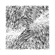
Figure 1: Convergence rate reference solution $\textbf{Q}^{\mbox{exact}}$ obtained using scheme OD1D. Colors indicate alignment with the dominant eigenvector. Dominant eigenvector is shown with black lines. The color bar for the remaining figures is given on the right.

4.2 Numerical Dissipation

In this example we study the evolution of the energy and numerical dissipation introduced by each scheme. We consider the domain $\Omega=[0,4]^{2}$ discretized into $50\times 50$ triangular elements, and final time $T=1.0$. For these simulations we use $\varepsilon=10^{-3}$. The initial condition is

$$\begin{array}[]{rcl}\displaystyle\mathbf{d}_{0}&=&\displaystyle\left(\cos\left(4\mbox{atan}2(x-2,y-2)\right),\sin\left(4\mbox{atan}2(x-2,y-2)\right),0\right)^{T}\,,\\ \vskip 6.0pt plus 2.0pt minus 2.0pt\cr\displaystyle\textbf{Q}_{0}&=&\displaystyle\frac{\mathbf{d}_{0}\mathbf{d}_{0}^{T}}{|\mathbf{d}_{0}|^{2}}-\frac{1}{3}\mathbf{I}\,.\end{array}$$ (51)

Here, $\mbox{atan2}(x,y)$ is the two argument tangent function. We will impose Neumann boundary conditions $\partial_{\mathbf{n}}\textbf{Q}=\bm{0}$.
For each numerical scheme, a sequence of time steps $\Delta t=\left\{\mbox{4e-4,2e-4,1e-4}\right\}$ is considered and the discrete energy and numerical dissipation is computed at each time step. The dynamics computed with the finest time step using scheme OD1D can be seen in Figure 2.
Figures 3 to 5 show the time evolution of the energy (top row) and the numerical dissipation (bottom row) for each numerical scheme. We can observe the energy is decreasing over the whole time interval, and in Figure 4 and Figure 5 a sharp decrease happens in the energy following the annihilation of all defects around time $t=0.35$ (see Figure 2). The numerical dissipation (bottom row) is always positive for the energy stable scheme UES1D, however, schemes OD2C and OD1D introduce much less dissipation. In fact, the dissipation introduced by scheme UES1D is so large, that the dynamics have been slowed down. We note that the time axis in Figure 3 is 20 times longer than in the case of the other two schemes. It is only the case of the finest time step $\Delta t=1e-4$ that the solution gets close to annihilating the defects which corresponds with the increased numerical dissipation after time $t=15$.
In Figure 6 we compare the dynamics obtained using scheme UES1D with different values of the stabilization constants $S_{1}$ and $S_{3}$. Specifically, we try the values given in 14 where $S_{1}=848$, and $S_{3}=208$, and compare to $S_{1}=100,$ $S_{3}=20$, and $S_{1}=10$, $S_{3}=2$. In the figure we can see that larger values of the stabilization parameters will slow the dynamics, and it is only in the third case that we observe the same sharp decrease in the energy corresponding to defect annihilation as was present in Figures 4 and 5. The numerical dissipation introduced at the same time can bee seen to rise to over 600 which is much larger that what was introduce by scheme OD2C ($\leq 30$) and scheme OD1D ( $\leq 150$). In Figure 7 we show the results obtained with each scheme on the same plot. The values shown for scheme UES1D in Figure 7 correspond to the case of the smallest stabilization constants in the previous figure.
In Table 7 we compare the computational time needed for each scheme to complete $10,000$ iterations using the same standard desktop computer. In this case, the decoupling of the unknowns in scheme OD1D saves nearly two thirds of the computational time from scheme OD2C. Furthermore, the truncation procedure for scheme UES1D is computationally inefficient resulting in the longest time to compute 10,000 iterations. It also should be noted that the slowed dynamics caused by the high numerical dissipation of scheme UES1D necessitated running the simulation over a larger time interval which increases the required number of iterations, hence the computational cost of the energy stable scheme is even greater.

Scheme	UES1D	OD2C	OD1D
Run Time (seconds)	209,959	34,846	13,490

Table 7: The time for each scheme to compute 10,000 iterations for the experiment given by (51)

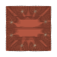
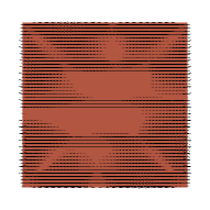
Figure 2: Defect dynamics using scheme OD1D in 2D with Neumann boundary conditions at times $t=0.01,0.1,0.25,0.35,0.5,1.0$. Color represents the difference of the two largest eigenvalues of Q and indicates the alignment of the nematic with the dominant eigenvector shown as black lines.

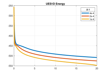
Figure 3: Top row: the energy of the system computed with scheme UES1D for different time steps. Left shows the energy over the whole time interval, and right a zoomed in view of the energy on the time interval $[0.3,0.5]$. Bottom row: the numerical dissipation for different time steps. Left shows the numerical dissipation over the whole time interval, and right shows a zoomed in view over the time interval $[0.3,0.5]$.

Figure 4: Top row: the energy of the system computed with scheme OD2C for different time steps. Left shows the energy over the whole time interval, and right a zoomed in view of the energy on the time interval $[0.3,0.5]$. Bottom row: the numerical dissipation for different time steps. Left shows the numerical dissipation over the whole time interval, and right shows a zoomed in view over the time interval $[0.3,0.5]$.

Figure 5: Top row: the energy of the system computed with scheme OD1D for different time steps. Left shows the energy over the whole time interval, and right a zoomed in view of the energy on the time interval $[0.3,0.5]$. Bottom row: the numerical dissipation for different time steps. Left shows the numerical dissipation over the whole time interval, and right shows a zoomed in view over the time interval $[0.3,0.5]$.

Figure 6: Energy and numerical dissipation of a solution computed using scheme UES1D with different values for stabilization constants $S_{1}$ and $S_{3}$.

Figure 7: Comparing energy and numerical dissipation as a result of each scheme. Scheme UES1D corresponds to the case of the smallest stabilization constants in Figure 6. Left shows the curves on the whole time interval. Right shows the same curves in in the time interval $[0.3,0.5]$.

Remark 15.

In the previous two examples we showed that scheme OD1D has equal or better convergence as scheme UES1D while also possessing the higher order numerical dissipation of scheme OD2C. Moreover, scheme OD1D is the most computationally efficient. Therefore, for the numerical experiments moving forward we will be using only scheme OD1D.

4.3 Defect Dynamics in 2D

This example is to show the evolution of defects in 2D subject to different boundary conditions. We use the same initial conditions (51) from the previous example and change the final time $T=3.5$. The case of Neumann boundary conditions is shown in Figure 2. Here, we see the presence of eight $\pm\left.1\right/\left.2\right.$ defects which move to and escape through the boundary.
Next, we impose the following Dirichlet boundary conditions

$$\mathbf{d}_{D}\,=\,\displaystyle(0,1,0)^{T}\,,\quad\quad\textbf{Q}_{D}\,=\,\mathbf{d}_{D}\mathbf{d}_{D}^{T}-\frac{1}{3}\mathbf{I}\,,\quad\quad\textbf{Q}\mid_{\partial\Omega}\,=\,\textbf{Q}_{D}\,.$$ (52)

The time evolution of the solution is shown in Figure 8. We note for this case that the boundary conditions induce the presence of more defects, which move towards the center and annihilate with the original eight defects. The final configuration shows uniform orientation coinciding with the boundary conditions.

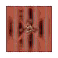
Figure 8: Defect dynamics in 2D with Dirichlet boundary conditions at times $t=0.01,0.05,0.1,0.2,0.3,1.0,2.5,3.0$. The color represents the difference of the two largest eigenvalues of Q and indicates the alignment of the nematic with the dominant eigenvector shown as black lines.

Finally, we impose a different set of Dirichlet boundary conditions as follows

$$\widetilde{\mathbf{d}_{D}}\,=\,\displaystyle\left(\frac{1}{2}(x-2),\frac{1}{2}(y-2),0\right)^{T}\,,\quad\quad\widetilde{\textbf{Q}_{D}}\,=\,\widetilde{\mathbf{d}_{D}}\widetilde{\mathbf{d}_{D}}^{T}-\frac{|\widetilde{\mathbf{d}_{D}}|^{2}}{3}\mathbf{I}\,,\quad\quad\textbf{Q}\mid_{\partial\Omega}\,=\,\widetilde{\textbf{Q}_{D}}\,.$$ (53)

The time evolution of the solution for this simulation can be seen in Figure 9. Here, we also note the production of defects from the boundary conditions. However, in contrast to the last simulation, the last two remaining defects are stabilized by the boundary conditions. These defects move slowly relative the motion of defects earlier in the simulation.
In Figure 10 we compare the dynamics of the solutions obtained using the three different boundary conditions. We see that the final configuration of the case of Neumann boundary conditions and $\textbf{Q}_{D}$ is a uniform configuration of the director vectors, and thus the energy of these solutions are similar at the final time. In the case of the boundary condition $\textbf{Q}_{\tilde{D}}$ we see that the final configuration contains two defects, hence the energy of this solution is higher than the previous two.

Figure 9: Defect dynamics in 2D with Dirichlet boundary conditions at times $t=0.01,0.03,0.05,0.1,0.15,0.3,0.35,1.0,3.0$. The color represents the difference of the two largest eigenvalues of Q and indicates the alignment of the nematic with the dominant eigenvector shown as black lines.

Figure 10: Comparing energy and numerical dissipation as a result of each case of boundary conditions. Here, Dirichlet 1 corresponds to the boundary conditions given by (52) and Dirichlet 2 corresponds to (53). Right shows a view of the curve shown in the middle restricted to the interval $[0.1,1.1]$.

4.4 Dynamics in 3D

The purpose of this example is to show dynamics in three dimensions to provide an example of the efficiency of scheme OD1D. We choose as computational domain $\Omega=[0,2]^{3}$ which is discretized into a $50\times 50\times 50$ triangular mesh. The final time is $T=0.2$, and the time step is $\Delta t=10^{-4}$. In this case $\varepsilon=1.0$.
We use Neumann boundary conditions $\partial_{\mathbf{n}}\textbf{Q}=\bm{0}$ and an initial state chosen so that each component of the vector $\mathbf{d}_{0}$ is randomly distributed uniformly in $[-1,1]$ with $|\mathbf{d}_{0}|=1$, and

$$\textbf{Q}_{0}\,=\,\mathbf{d}_{0}\mathbf{d}_{0}^{T}-\frac{|\mathbf{d}_{0}|^{2}}{3}\mathbf{I}\,.$$ (54)

Figures 11 to 13 show the result of this simulation using scheme OD1D. Initially, a random orientation of the nematic throughout the domain, and as time progresses the system moves towards a uniform orientation. In Figure 11 we note the appearance, movement, and annihilation of defects on the surface of the domain. Figure 13 shows the time evolution of the energy, where we can observe that the energy is decreasing at all times.

Figure 11: Dynamics in 3D with random initial condition at $t=0.0001,0.01,0.02,0.03,0.04,0.05,0.065,0.1,$ and $0.125$. The color represents the difference of the two largest eigenvalues of Q and indicates the alignment of the nematic with the dominant eigenvector shown as black lines in Figure 12.

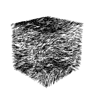
Figure 12: The eigenvector of Q corresponding to the largest eigenvalue at $t=0.0001,0.01,0.02,0.03,0.04,0.05,0.065,0.1,$ and $0.125$.

Figure 13: Time evolution of the energy for the three dimensional simulation computed using scheme OD1D. Right plot is the same curve in a limited y-axis window to better show the dynamics.

5 Conclusion

In this paper we have presented three different linear numerical schemes for a Q-tensor problem which can be used to study the dynamics of nematic liquid crystals efficiently in two and three dimensions. To summarize (see Table 8), scheme UES1D is an unconditionally energy stable decoupled scheme which is first order accurate in time. Next, we proposed scheme OD2C which is a second order accurate scheme that introduces considerably less numerical dissipation than scheme UES1D which allows for simulations more closely resembling the true dynamics of the system. Finally, scheme OD1D is a first order accurate decoupled scheme which retains the same second order numerical dissipation as in scheme OD2C while also being the most computationally efficient.
It is important to note that scheme UES1D is energy stable, however, from the simulations presented we see that this scheme is not ideal. The high numerical dissipation introduced by this scheme causes the simulated dynamics to be relatively slow which increases the computational cost. In addition, the truncation procedure further decreases the efficiency. Instead, it is scheme OD1D which we have shown to strike the best balance of accuracy and efficiency by presenting several simulations in two and three dimensions. This scheme provides researchers with a method for simulating nematic liquid, and a starting point for developing accurate and efficient numerical schemes for the larger Beris-Edwards system which incorporates hydrodynamic effects.

Scheme	Decoupled	Numerical Dissipation	Accuracy	Energy Stable
1	✓	$\mathcal{O}(\Delta t)$	$\mathcal{O}(\Delta t)$	✓
2		$\mathcal{O}(\Delta t^{2})$	$\mathcal{O}(\Delta t^{2})$
3	✓	$\mathcal{O}(\Delta t^{2})$	$\mathcal{O}(\Delta t)$

Table 8: Summary of the properties of the numerical schemes presented in this work.

Appendix

Here we write a few facts about derivatives that help to derive the terms involved in the numerical schemes. It is helpful to use repeated index notation so that

$$Q_{ij}Q_{jk}=\sum_{j}Q_{ij}Q_{jk}\,.$$

In addition, we use the Kronecker delta function

$$\delta_{ij}=\left\{\begin{array}[]{lr}1&\mbox{ if }i=j\,,\\ \cr 0&\mbox{ if }i\neq j\,.\end{array}\right.$$

Below we make use of the following relations for second order tensors

$$A_{ij}\delta_{jk}=A_{ik}\,,\quad\quad A_{ij}\delta_{ik}=A_{kj}\quad\quad\mbox{and}\quad\quad\frac{\partial A_{ij}}{\partial A_{kl}}=\delta_{ik}\delta_{jl}\,.$$

Derivatives of the potential function $\Psi(\textbf{Q})$

Let $F:\mathbb{R}^{3\times 3}\rightarrow\mathbb{R}$ be a scalar valued function of a second order tensor Q. Then $\bm{f}=\nabla_{\textbf{Q}}F$ is a second order tensor valued function and the second derivative $\nabla\bm{f}$ is a fourth order tensor valued function with the following indexing

$$\left[\bm{f}\right]_{ij}\,=\,\displaystyle\frac{\partial}{\partial Q_{ij}}f\quad\mbox{ and }\quad\left[\nabla\bm{f}\right]_{ijkl}\,=\,\displaystyle\frac{\partial}{\partial Q_{kl}}\left[\bm{f}\right]_{ij}\,.$$

First, let $F(\textbf{Q})=\texttt{tr}(\textbf{Q}^{2})$ as in the first term of the LdG potential function. Then we can write $F$ as

$$F(\textbf{Q})\,=\,\texttt{tr}(\textbf{Q}^{2})\,=\,Q_{ij}Q_{ij}$$

and so the derivatives become

$$\left[\bm{f}\right]_{pq}\,=\,\frac{\partial}{\partial Q_{pq}}Q_{ij}Q_{ij}\,=\,2Q_{ij}\frac{\partial Q_{ij}}{\partial Q_{pq}}\,=\,2Q_{ij}\delta_{ip}\delta_{jq}\,=\,2Q_{iq}\delta_{ip}\,=\,2Q_{pq}\Rightarrow\bm{f}\,=\,2\textbf{Q}\,.$$

Then the second derivative is

$$\left[\nabla\bm{f}\right]_{ijkl}\,=\,2\frac{\partial}{\partial Q_{kl}}Q_{ij}\,=\,2\delta_{ik}\delta_{jl}\,.$$

Next, we let $F(\textbf{Q})=\texttt{tr}(\textbf{Q}^{3})$. In repeated index notation this is

$$F(\textbf{Q})\,=\,\texttt{tr}(\textbf{Q}^{3})\,=\,Q_{ij}Q_{jk}Q_{ki}\,.$$

The first and second derivatives are

$$\left[\bm{f}\right]_{pq}\,=\,\frac{\partial}{\partial Q_{pq}}Q_{ij}Q_{jk}Q_{ki}\,=\,Q_{pk}Q_{kq}+Q_{pi}Q_{iq}+Q_{pj}Q_{jq}\,=\,3\left[\textbf{Q}^{2}\right]_{pq}\Rightarrow\bm{f}(\textbf{Q})\,=\,3\textbf{Q}^{2}\,,$$

$$\left[\nabla\bm{f}\right]_{ijkl}\,=\,3\frac{\partial}{\partial Q_{kl}}Q_{ip}Q_{pj}\,=\,3\left(\delta_{ik}\delta_{lp}Q_{pj}+Q_{ip}\delta_{pk}\delta_{jl}\right)\,=\,3\left(\delta_{ik}Q_{lj}+Q_{ik}\delta_{jl}\right)\,.$$

Finally, let $F(\textbf{Q})=\left(\texttt{tr}(\textbf{Q}^{2})\right)^{2}$. The first and second derivatives are

$$\left[\bm{f}\right]_{pq}\,=\,\frac{\partial}{\partial Q_{pq}}\left(Q_{ij}Q_{ij}\right)^{2}\,=\,2\left(Q_{ij}Q_{ij}\right)\frac{d}{dQ_{pq}}\left(Q_{ij}Q_{ij}\right)\,=\,4Q_{pq}\left(Q_{ij}Q_{ij}\right)\Rightarrow\bm{f}(\textbf{Q})\,=\,4\textbf{Q}\texttt{tr}(\textbf{Q}^{2})\,.$$

$$\left[\nabla\bm{f}\right]_{ijkl}\,=\,4\frac{\partial}{\partial Q_{kl}}\left[Q_{ij}\left(Q_{pq}Q_{pq}\right)\right]\,=\,4\left(\left(Q_{pq}Q_{pq}\right)\delta_{ik}\delta_{jl}+2Q_{ij}Q_{kl}\right)\,=\,4\left(\texttt{tr}(\textbf{Q}^{2})\delta_{ik}\delta_{jl}+2Q_{ij}Q_{kl}\right)\,.$$

For $\bm{p}(\textbf{Q})=\frac{1}{3}\texttt{tr}(\textbf{Q}^{2})\mathbf{I}$, we have the fourth order tensor $\nabla\bm{p}(\textbf{Q})$ which can be written as

$$\begin{array}[]{rcl}\nabla\bm{p}(\textbf{Q})&=&\mathbf{I}\otimes\textbf{Q}\end{array}$$

and

$$\left[\nabla\bm{p}(\textbf{Q})\right]_{ijkl}=\left\{\begin{array}[]{ll}2Q_{kl}&\mbox{ if }i=j\,,\\ 0&\mbox{ otherwise}\,.\end{array}\right.$$

Hence when $|\textbf{Q}|\leq\alpha$ we have

$$\left|\left|\left[\nabla\bm{p}(\textbf{Q})\right]_{ijkl}\right|\right|_{L^{\infty}}\,\leq\,2\alpha\,,\quad\quad\left|\left|\nabla\bm{p}(\textbf{Q})\right|\right|_{F}\,\leq\,108\alpha^{2}\,.$$

From Cubic to Quadratic Growth

Here we derive the bounds for the truncated potential function (25). Let $\beta=(\alpha_{2}-\alpha_{1})^{-1}$. The first and second derivatives are

$$\left[\nabla\rho(\texttt{tr}(\textbf{Q}^{2})\right]_{ij}\,=\,-12\beta^{2}\textbf{Q}_{ij}\left(1-\left(|Q|^{2}-\alpha_{1}\right)\right)\left(|Q|^{2}-\alpha_{1}\right)$$

and

$$\begin{array}[]{rcl}\displaystyle\left[\bm{H}_{\rho}(\texttt{tr}(\textbf{Q}^{2})\right]_{ijkl}&=&-12\beta^{2}\left[-\beta\delta_{ik}\delta_{jl}\left(|Q|^{2}\right)^{2}-\beta|Q|^{2}Q_{ij}Q_{kl}\right.\\ \cr&&\quad\displaystyle\left.+(1+2\alpha_{1}\beta)\left(|Q|^{2}\delta_{ik}\delta_{jl}+Q_{ij}Q_{kl}\right)-\alpha_{1}\beta(1+\alpha_{1})\delta_{ik}\delta_{jl}\right]\,.\end{array}$$

Hence when $\alpha_{1}<|\textbf{Q}|<\alpha_{2}$, we have $Q_{ij}\leq\alpha_{2}$ for all $i,j=1,2,3$, so

$$\left|\left[\nabla\rho(\textbf{Q})\right]_{ij}\right|\leq 12\beta^{2}\left(\alpha_{2}^{5}+(1+2\alpha_{1})\alpha_{2}^{2}+\alpha_{1}^{2}+\alpha_{1}\right)$$

and

$$\left|\left[H_{\rho}\right]_{ijkl}\right|\leq 24\alpha_{2}^{4}\beta^{3}+3\alpha_{2}^{2}+6\alpha_{1}\alpha_{2}^{2}\beta+\alpha_{1}^{2}\beta+\alpha_{1}\beta\,.$$

Therefore, we see that $\left|\left[H_{\rho}\right]_{ijkl}\right|$ grows without bound as $\alpha_{2}\rightarrow\infty$ or $\beta\rightarrow\infty$. Now we detail the derivatives of $\widehat{\psi}(\textbf{Q})$:

$$\begin{array}[]{rcl}\displaystyle\left[\bm{\widehat{\psi}}_{3}(\textbf{Q})\right]_{ij}&=&\left[\bm{\widehat{\psi}}_{3}(\textbf{Q})\right]_{ij}\rho(\texttt{tr}(\textbf{Q}^{2}))+\widehat{\Psi}_{3}(\textbf{Q})\left[\nabla\rho(\texttt{tr}(\textbf{Q}^{2}))\right]_{ij}\\ \cr\displaystyle\hfil&+&2C^{2}Q_{ij}(1-\rho(\texttt{tr}(\textbf{Q}^{2}))-C^{2}Q_{pq}Q_{pq}\left[\nabla\rho(\texttt{tr}(\textbf{Q}^{2}))\right]_{ij}\end{array}$$

and

$$\begin{array}[]{rcl}\displaystyle\left[\nabla\bm{\widehat{\psi}}_{3}(\textbf{Q})\right]_{ijkl}&=&\left[\bm{\widehat{\psi}}_{3}(\textbf{Q})\right]_{ij}\left[\nabla\rho(\texttt{tr}(\textbf{Q}^{2}))\right]_{kl}+\left[\bm{\widehat{\psi}}_{3}(\textbf{Q})\right]_{kl}\left[\nabla\rho(\texttt{tr}(\textbf{Q}^{2}))\right]_{ij}\\ \cr\displaystyle\hfil&+&\rho(\texttt{tr}(\textbf{Q}^{2}))\left[\nabla\bm{\widehat{\psi}}_{3}(\textbf{Q})\right]_{ijkl}+\widehat{\Psi}_{3}(\textbf{Q})\left[\bm{H}_{\rho}(\texttt{tr}(\textbf{Q}^{2}))\right]_{ijkl}\\ \cr\displaystyle\hfil&+&2C^{2}\delta_{ik}\delta_{jl}(1-\rho(\texttt{tr}(\textbf{Q}^{2}))+2C^{2}Q_{ij}\left[\bm{\widehat{\psi}}_{3}(\textbf{Q})\right]_{kl}\\ \cr\displaystyle\hfil&-&2C^{2}Q_{kl}\left[\bm{\widehat{\psi}}_{3}(\textbf{Q})\right]_{ij}-C^{2}Q_{pq}Q_{pq}\left[\bm{H}_{\rho}(\texttt{tr}(\textbf{Q}^{2}))\right]_{ijkl}\,.\end{array}$$

Since we have the following bounds for $\widehat{\Psi}_{3}$ when $\alpha_{1}\leq|\textbf{Q}|\leq\alpha_{2}$

$$\left|\left[\bm{\widehat{\psi}}_{3}(\textbf{Q})\right]_{ij}\right|\leq B\alpha_{2}^{2}$$

and

$$\left|\left[\nabla\bm{\widehat{\psi}}_{3}\right]_{ijkl}\right|\leq 2B\alpha_{2}\,,$$

we have the following bound for $\widehat{\psi}(\textbf{Q})$

$$\begin{array}[]{rcl}\displaystyle\left|\left[\nabla\bm{\widehat{\psi}}_{3}\right]_{ijkl}\right|&\leq&24B\alpha_{2}\beta\left(\alpha_{2}^{5}+\alpha_{2}^{2}(1+2\alpha_{1})+\alpha_{1}^{2}+\alpha_{1}\right)\\ \cr&&\displaystyle+2B\alpha_{2}\left(3\beta\alpha_{2}^{2}+3\beta\alpha_{1}+2\alpha_{2}^{4}\beta^{2}+4\alpha_{1}\alpha_{2}^{2}\beta^{2}+2\alpha_{1}^{2}\beta^{2}+1\right)\\ \cr&&\displaystyle+648B\alpha_{2}^{7}\beta^{3}+81B\alpha_{2}^{5}+162B\alpha_{2}^{5}\beta\alpha_{1}+27B\alpha_{2}^{3}\beta\alpha_{1}^{2}+27B\alpha_{2}^{3}\beta\alpha_{1}\\ \cr&&\displaystyle+2C^{2}\left(3\beta\alpha_{2}^{2}+3\beta\alpha_{1}+2\beta^{2}\alpha_{2}^{4}+2\beta^{2}\alpha_{1}^{2}+4\beta^{2}\alpha_{2}^{2}\alpha_{1}+2\right)\\ \cr&&\displaystyle+C^{2}\alpha_{2}^{2}\left(4B\alpha_{2}+24\alpha_{2}^{4}+3\alpha_{2}^{2}+6\alpha_{2}^{2}\alpha_{1}\beta+\alpha_{1}^{2}\beta+\beta\alpha_{1}\right)\,.\end{array}$$

In particular, if $\alpha=1.18<\alpha_{1}=1.19<\alpha_{2}=1.2$, then

$$\left\|\left[\nabla\bm{\widehat{\psi}}_{3}\right]_{ijkl}\right\|_{L^{\infty}}\leq 3619\quad\mbox{ and }\quad\|\nabla\bm{\widehat{\psi}}_{3}\|_{F}\leq 32571\,.$$

References

- [1] Helmut Abels, Georg Dolzmann and Yuning Liu “Strong solutions for the Beris-Edwards model for nematic liquid crystals with homogeneous Dirichlet boundary conditions” In Advances in Differential Equations 21, 2013 DOI: 10.57262/ade/1448323166
- [2] Helmut Abels, Georg Dolzmann and YuNing Liu “Well-posedness of a fully coupled Navier-Stokes/Q-tensor system with inhomogeneous boundary data” In SIAM Journal on Mathematical Analysis 46.4 SIAM, 2014, pp. 3050–3077 DOI: 10.1137/130945405
- [3] James Paul Ahrens, Berk Geveci and C. Charles Law “ParaView: An End-User Tool for Large-Data Visualization” In The Visualization Handbook, 2005 URL: https://api.semanticscholar.org/CorpusID:56558637
- [4] John M Ball “Mathematics and liquid crystals” In Molecular Crystals and Liquid Crystals 647.1 Taylor & Francis, 2017, pp. 1–27 DOI: 10.1080/15421406.2017.1289425
- [5] A.N. Beris and B.J. Edwards “Thermodynamics of Flowing Systems: with Internal Microstructure”, Oxford Engineering Science Series Oxford University Press, 1994 URL: https://books.google.com/books?id=dqxFUy7_vhsC
- [6] Juan Pablo Borthagaray and Shawn W. Walker “Chapter 5 - The Q-tensor model with uniaxial constraint” In Geometric Partial Differential Equations - Part II 22, Handbook of Numerical Analysis Elsevier, 2021, pp. 313–382 DOI: 10.1016/bs.hna.2020.09.001
- [7] Lucas Bouck, Ricardo Nochetto and Vladimir Yushutin “A Hydrodynamical Model of Nematic Liquid Crystal Films with a General State of Orientational Order” In Journal of Nonlinear Science 34, 2023 DOI: 10.1007/s00332-023-09970-6
- [8] R. C. Cabrales, F. Guillén-González and J. V. Gutiérrez-Santacreu “A Time-Splitting Finite-Element Stable Approximation for the Ericksen-Leslie Equations” In SIAM Journal on Scientific Computing 37.2, 2015, pp. B261–B282 DOI: 10.1137/140960979
- [9] Yongyong Cai, Jie Shen and Xiang Xu “A stable scheme and its convergence analysis for a 2D dynamic Q-tensor model of nematic liquid crystals” In Mathematical Models and Methods in Applied Sciences 27, 2017 DOI: 10.1142/S0218202517500245
- [10] Hai-Wei Chen et al. “Liquid crystal display and organic light-emitting diode display: present status and future perspectives” In Light: Science & Applications 7.3 Nature Publishing Group, 2018, pp. 17168–17168 DOI: 10.1038/lsa.2017.168
- [11] Mei Chen et al. “Recent Advances in 4D Printing of Liquid Crystal Elastomers” In Advanced Materials Wiley Online Library, 2023, pp. 2209566 DOI: 10.1002/adma.202209566
- [12] Blanca Climent-Ezquerra and Guill’en-Gonz’alez Francisco “Long-Time Behavior of Global Weak Solutions for a Beris-Edwards Type Model of Nematic Liquid Crystals” In Journal of Mathematical Fluid Mechanics 24, 2022 DOI: 10.1007/s00021-022-00730-2
- [13] M. Cunha, M. G. Debije and A. P. H. J. Schenning “Bioinspired light-driven soft robots based on liquid crystal polymers” In Chem. Soc. Rev. 49 The Royal Society of Chemistry, 2020, pp. 6568–6578 DOI: 10.1039/D0CS00363H
- [14] Jerald Laverne Ericksen “Hydrostatic theory of liquid crystals” In Archive for Rational Mechanics and Analysis 9, 1962, pp. 371–378 DOI: 10.1007/BF00253358
- [15] JL Ericksen “Equilibrium theory of liquid crystals” In Advances in liquid crystals 2 Elsevier, 1976, pp. 233–298
- [16] F. C. Frank “I. Liquid crystals. On the theory of liquid crystals” In Discuss. Faraday Soc. 25 The Royal Society of Chemistry, 1958, pp. 19–28 DOI: 10.1039/DF9582500019
- [17] P.G. Gennes and J. Prost “The Physics of Liquid Crystals”, International Series of Monographs on Physics Clarendon Press, 1993 URL: https://books.google.com/books?id=0Nw-dzWz5agC
- [18] Yuezheng Gong, Jia Zhao and Qi Wang “Arbitrarily high-order unconditionally energy stable SAV schemes for gradient flow models” In Computer Physics Communications 249, 2020, pp. 107033 DOI: https://doi.org/10.1016/j.cpc.2019.107033
- [19] Yuezheng Gong, Jia Zhao and Qi Wang “Arbitrarily High-Order Unconditionally Energy Stable Schemes for Thermodynamically Consistent Gradient Flow Models” In SIAM Journal on Scientific Computing 42.1, 2020, pp. B135–B156 DOI: 10.1137/18M1213579
- [20] Varun M. Gudibanda, Franziska Weber and Yukun Yue “Convergence Analysis of a Fully Discrete Energy-Stable Numerical Scheme for the Q-Tensor Flow of Liquid Crystals” In SIAM Journal on Numerical Analysis 60.4, 2022, pp. 2150–2181 DOI: 10.1137/20M1383550
- [21] Francisco Guillén-González and María Ángeles Rodríguez-Bellido “Weak solutions for an initial-boundary Q-tensor problem related to liquid crystals” In Nonlinear Analysis: Theory, Methods & Applications 112, 2015, pp. 84–104 DOI: 10.1016/j.na.2014.09.011
- [22] Francisco Guillén-González and Giordano Tierra “Second order schemes and time-step adaptivity for Allen-Cahn and Cahn-Hilliard models” In Computers & Mathematics with Applications 68.8, 2014, pp. 821–846 DOI: 10.1016/j.camwa.2014.07.014
- [23] Frédéric Hecht “New development in freefem++” In J. Num. Math., 2012 URL: https://api.semanticscholar.org/CorpusID:12770876
- [24] The MathWorks Inc. “MATLAB version: 9.13.0 (R2022b)” Natick, Massachusetts, United States: The MathWorks Inc., 2022 URL: https://www.mathworks.com
- [25] Jan P. F. Lagerwall and Giusy Scalia “A new era for liquid crystal research: Applications of liquid crystals in soft matter nano-, bio- and microtechnology” In Current Applied Physics 12, 2012, pp. 1387–1412 DOI: 10.1016/J.CAP.2012.03.019
- [26] F. M. Leslie “Some Constitutive Equations for Anisotropic Fluids” In The Quarterly Journal of Mechanics and Applied Mathematics 19.3, 1966, pp. 357–370 DOI: 10.1093/qjmam/19.3.357
- [27] Frank Matthews Leslie “Some constitutive equations for liquid crystals” In Archive for Rational Mechanics and Analysis 28, 1968, pp. 265–283 DOI: 10.1007/BF00251810
- [28] Xiao Li et al. “Directed Self-Assembly of Colloidal Particles onto Nematic Liquid Crystalline Defects Engineered by Chemically Patterned Surfaces” In ACS Nano 11.6, 2017, pp. 6492–6501 DOI: 10.1021/acsnano.7b03641
- [29] Apala Majumdar “Equilibrium order parameters of nematic liquid crystals in the Landau-de Gennes theory” In European Journal of Applied Mathematics 21.2, 2010, pp. 181–203 DOI: 10.1017/S0956792509990210
- [30] Nigel J. Mottram and Christopher J. P. Newton “Introduction to Q-tensor theory”, 2014 arXiv:1409.3542 [cond-mat.soft]
- [31] C. W. Oseen “The theory of liquid crystals” In Trans. Faraday Soc. 29 The Royal Society of Chemistry, 1933, pp. 883–899 DOI: 10.1039/TF9332900883
- [32] Marius Paicu and Arghir Zarnescu “Energy dissipation and regularity for a coupled Navier-Stokes and Q-tensor system” In Archive for Rational Mechanics and Analysis 203 Springer, 2012, pp. 45–67 DOI: 10.1007/s00205-011-0443-x
- [33] Tejal Pawale et al. “Dynamic Motions of Topological Defects in Nematic Liquid Crystals under Spatial Confinement” In Advanced Materials Interfaces 10.15, 2022, pp. 2300136 DOI: 10.1002/admi.202300136
- [34] Devin Roach et al. “Long Liquid Crystal Elastomer Fibers with Large Reversible Actuation Strains for Smart Textiles and Artificial Muscles” In ACS Applied Materials & Interfaces 11, 2019 DOI: 10.1021/acsami.9b04401
- [35] Cody D. Schimming, Jorge Viñals and Shawn W. Walker “Numerical method for the equilibrium configurations of a Maier-Saupe bulk potential in a Q-tensor model of an anisotropic nematic liquid crystal” In Journal of Computational Physics 441, 2021, pp. 110441 DOI: 10.1016/j.jcp.2021.110441
- [36] Jie Shen, Jie Xu and Jiang Yang “A New Class of Efficient and Robust Energy Stable Schemes for Gradient Flows” In SIAM Review 61, 2017 DOI: 10.1137/17M1150153
- [37] A.M. Sonnet and E.G. Virga “Dissipative Ordered Fluids: Theories for Liquid Crystals”, Surveys and Tutorials in the Applied Mathematical Sciences Springer New York, 2012 URL: https://books.google.com/books?id=HNL3sd669qUC
- [38] Thomas M. Surowiec and Shawn W. Walker “Optimal Control of the Landau-de Gennes Model of Nematic Liquid Crystals” In SIAM Journal on Control and Optimization 61.4, 2023, pp. 2546–2570 DOI: 10.1137/22M1506158
- [39] Weber, Franziska and Yue, Yukun “On the convergence of an IEQ-based first-order semi-discrete scheme for the Beris-Edwards system” In ESAIM: M2AN 57.6, 2023, pp. 3275–3302 DOI: 10.1051/m2an/2023071
- [40] Scott Woltman, Gregory Jay and Gregory Crawford “Liquid-crystal materials find a new order in biomedical applications” In Nature materials 6, 2008, pp. 929–38 DOI: 10.1038/nmat2010
- [41] Xiang Xu “Recent analytic development of the dynamic Q-tensor theory for nematic liquid crystals” In Electronic Research Archive 30.6, 2022 DOI: 10.3934/era.2022113
- [42] Jia Zhao, Xiaofeng Yang, Yuezheng Gong and Qi Wang “A novel linear second order unconditionally energy stable scheme for a hydrodynamic Q-tensor model of liquid crystals” In Computer Methods in Applied Mechanics and Engineering 318, 2017, pp. 803–825 DOI: https://doi.org/10.1016/j.cma.2017.01.031
- [43] Jia Zhao, Xiaofeng Yang, Jun Li and Qi Wang “Energy Stable Numerical Schemes for a Hydrodynamic Model of Nematic Liquid Crystals” In SIAM Journal on Scientific Computing 38, 2016, pp. A3264–A3290 DOI: 10.1137/15M1024093