An Analysis of Switchback Designs in Reinforcement Learning

Qianglin Wen1, Chengchun Shi2 , Ying Yang3, Niansheng Tang1 & Hongtu Zhu4
1Yunnan University, 2London School of Economics and Political Science
3Academy of Mathematics and Systems Science, Chinese Academy of Sciences
4University of North Carolina at Chapel Hill
The first two authors contribute equally to this paper.The last two authors are senior authors of this paper. Address for correspondence: Hongtu Zhu, Ph.D., E-mail: htzhu@email.unc.edu.

Abstract

This paper offers a detailed investigation of switchback designs in A/B testing, which alternate between baseline and new policies over time. Our aim is to thoroughly evaluate the effects of these designs on the accuracy of their resulting average treatment effect (ATE) estimators. We propose a novel “weak signal analysis” framework, which substantially simplifies the calculations of the mean squared errors (MSEs) of these ATEs in Markov decision process environments. Our findings suggest that (i) when the majority of reward errors are positively correlated, the switchback design is more efficient than the alternating-day design which switches policies in a daily basis. Additionally, increasing the frequency of policy switches tends to reduce the MSE of the ATE estimator. (ii) When the errors are uncorrelated, however, all these designs become asymptotically equivalent. (iii) In cases where the majority of errors are negative correlated, the alternating-day design becomes the optimal choice. These insights are crucial, offering guidelines for practitioners on designing experiments in A/B testing. Our analysis accommodates a variety of policy value estimators, including model-based estimators, least squares temporal difference learning estimators, and double reinforcement learning estimators, thereby offering a comprehensive understanding of optimal design strategies for policy evaluation in reinforcement learning.

Key words: A/B testing; policy evaluation; reinforcement learning; switchback designs.

1 Introduction

Over recent decades, policy evaluation has become increasingly important in various fields such as economics (Athey and Imbens, 2017), medicine (Yu et al., 2021), environmental science (Reich et al., 2021), and epidemiology (Hudgens and Halloran, 2008). In the technology sector, major companies like Google, Amazon, Netflix, and Microsoft extensively use policy evaluation methods, particularly A/B testing, to measure and improve the effectiveness of new products or strategies against established ones (see e.g., Johari et al., 2017; Yang et al., 2017; Waudby-Smith et al., 2022; Wan et al., 2023). An illustrative example of policy evaluation in practice can be seen in ridesourcing platforms like Uber, Lyft111https://eng.lyft.com/experimentation-in-a-ridesharing-marketplace-b39db027a66e, and Didi. These companies constantly develop and refine policies for order dispatching and subsidies, aiming to optimize some key performance metrics such as supply-demand equilibrium, driver earnings, response rates, and order completion rates (Qin et al., 2022). Accurate policy evaluation is vital for identifying the most effective strategies to enhance the efficiency and convenience of the transportation system. A/B testing is a common tool used by these companies for real-time experiments to assess various policy impacts (Xu et al., 2018; Tang et al., 2019; Zhou et al., 2021).

Challenges. In numerous scenarios, treatments are assigned over time in a sequential manner (Robins, 1986; Bojinov and Shephard, 2019; Viviano and Bradic, 2023), presenting unique challenges for policy evaluation. A primary issue is that previous treatments can significantly influence future outcomes, a factor often overlooked by traditional A/B testing and policy evaluation methods which typically do not consider such carryover effects (Ni et al., 2023). For instance, in ridesharing, the implementation of a specific order dispatch policy at one time can change the spatial distribution of drivers in a city, impacting subsequent outcomes (see e.g., Li et al., 2024, Figure 2). Additionally, standard methods like the two-sample $t$-test often fail to capture these effects, frequently resulting in insignificant p-values (Shi et al., 2023, Section 5). Another challenge is the limited sample size in many applications, coupled with generally modest treatment effects. This issue is particularly prevalent in online experiments in ridesharing, which seldom last more than two weeks and typically exhibit effect sizes ranging from $0.5\%$ to $2\%$ (Xu et al., 2018; Tang et al., 2019). To address these challenges, it is crucial to develop new theories and methods that can enhance online experimentation and policy evaluation.

Contributions. This paper conducts a quantitative analysis to understand the effects of various switchback designs on the precision of their resulting policy value estimators. Switchback designs alternates between a baseline and a new policy at fixed intervals. Each policy is implemented for a specified duration before transitioning to the other. When the duration of each policy extends to a full day, the design becomes an “alternating-day” design, involving daily policy switches. Switchback designs are increasingly utilized in large-scale ridesharing platforms (Qin et al., 2022). Luo et al. (2024) has empirically demonstrated that more frequent policy alternations can reduce mean squared error (MSE) in estimating the average treatment effect (ATE). However, the mechanisms driving the improvement in estimation accuracy lack thorough exploration in existing research.

Our study fills this gap by offering a comprehensive theoretical analysis within a reinforcement learning (RL, Sutton and Barto, 2018) framework, where data follows a Markov decision process (MDP, Puterman, 2014) model. When the treatment effect signal is weak, we show that:

  1. (i)

    In scenarios with positively correlated reward errors, the precision of the ATE estimator tends to be improved with more frequent alternations between policies. Notably, this leads us to an intriguing conclusion: the off-policy ATE estimator under switchback designs outperforms its on-policy counterpart under the alternating-day design in terms of estimation efficiency. This conclusion remains valid even in the presence of some negatively correlated errors. The superior efficiency of the switchback design is attributed to the switchback design’s inherent capability to neutralize the influence of autocorrelated errors over time, thereby producing a more accurate estimator. This insight has not been systematically documented in existing literature, to our knowledge. We also remark that positively autocorrelated errors are commonly observed in practice, as demonstrated in Figure 1.

  2. (ii)

    When reward errors are uncorrelated, all designs become asymptotically equivalent.

  3. (iii)

    When the majority of errors are negatively correlated, the alternating-day design becomes the most efficient.

The weak signal assumption is consistent with the moderate treatment effect observed in practical situations, indicating that this assumption is likely to hold.

Refer to caption
Refer to caption
Figure 1: The estimated correlation coefficients between pairs of fitted reward residuals, utilizing two real datasets originating from two distinct cities. It is evident that a majority of the residual pairs exhibit positive correlation. The diagonal components have been omitted to enhance clarity.

Central to our study is the introduction of the “weak signal analysis”. This innovative approach substantially streamlines the computations associated with the MSEs of various ATE estimators in RL, allowing our theoretical results to accommodate various policy value estimators, including model-based estimators, least squares temporal difference learning estimators, and double reinforcement learning estimators (see Uehara et al., 2022, for a review). To validate our theoretical claims empirically, we conduct extensive numerical simulations that leverage real-world data from ridesharing platforms.

1.1 Related works

Our paper intersects with three related lines of research: A/B testing, off-policy evaluation (OPE) and experimental designs.

A/B testing. A/B testing has emerged as the gold standard for product development, gaining widespread adoption across various technology companies (see Larsen et al., 2023; Quin et al., 2024, for reviews). The foundational principle of A/B testing relies on the application of causal inference techniques to estimate the treatment effect of a new intervention. This is typically done under the assumption of “no interference”, which partly aligns with the stable unit treatment value assumption (SUTVA, Rubin, 2005). As commented earlier, the assumption of “no interference” can be violated in time series experiments that involve sequential decision making over time. Consequently, most existing A/B testing solutions are not applicable to infer the treatment effects under switchback designs.

Off-policy evaluation. Our work is closely related to the literature on OPE in RL, whose objective is to estimate the expected return of a new target policy based on data collected by a different behavior policy in sequential decision making. Current methodologies in this field generally fall into one of two categories: model-based and model-free approaches. Model-based methods fit an MDP model from the offline data, followed by computing the policy value based on the estimated model (Gottesman et al., 2019; Yin and Wang, 2020; Wang et al., 2024). On the other hand, model-free methods can be further classified into several subtypes. Value-based approaches focus on estimating the policy value via an estimated Q-function or value function (Luckett et al., 2019; Hao et al., 2021; Liao et al., 2021; Chen and Qi, 2022; Farias et al., 2022; Shi et al., 2022; Li et al., 2023; Liu et al., 2023). Importance sampling (IS) methods adjust the observed rewards by the density ratio between the target and behavior policies, effectively accounting for the distributional shift between them (Zhao et al., 2012; Thomas et al., 2015; Chen et al., 2016; Wang et al., 2018; Hanna et al., 2019; Wang et al., 2023; Hu and Wager, 2023; Thams et al., 2023). Doubly-robust methods represent a more advanced strand, combining both value-based and IS methods to achieve a more robust evaluation of policy value (Zhang et al., 2013; Jiang and Li, 2016; Thomas and Brunskill, 2016; Bibaut et al., 2019; Uehara et al., 2020; Kallus and Uehara, 2022; Liao et al., 2022). Our theories cover model-based, value-based and doubly-robust estimators, offering a comprehensive analysis.

Despite the popularity of developing advanced OPE estimators, the strategies for generating offline data to maximize their estimation efficiency have not been thoroughly investigated. Existing works either focus on a contextual bandit setting where the carryover effect does not exist (Wan et al., 2022) or do not study switchback designs (Hanna et al., 2017; Mukherjee et al., 2022; Zhong et al., 2022; Li et al., 2023). This gap is where the focus of our paper comes into play. We aim to explore how switchback designs can impact the efficiency of policy value estimators, thereby enriching the OPE literature.

Experimental design. There exists a rich literature on experimental design tailored for clinical trials, featuring a range of optimal designs (Begg and Iglewicz, 1980; Wong and Zhu, 2008; Jones and Goos, 2009; Atkinson and Pedrosa, 2017; Rosenblum et al., 2020) and sequential adaptive designs (Hu et al., 2009; Baldi Antognini and Zagoraiou, 2011; Atkinson and Biswas, 2013; Hu et al., 2015). These methods are developed under the classical identically and independently distributed setting. Recent developments have expanded the scope to accommodate spatial or network spillover effects (Ugander et al., 2013; Li et al., 2019; Kong et al., 2021; Leung, 2022) and to address the complex interactions inherent in two-sided marketplaces (Bajari et al., 2021; Johari et al., 2022). Despite these advancements, a gap remains in the literature concerning designs that adequately account for temporal carryover effects in sequential decision making.

Recent studies such as Hu and Wager (2022), Xiong et al. (2023) and Bojinov et al. (2023) investigated switchback designs in temporal experiments, but several key distinctions exist between their work and our proposal.

  1. (i)

    A key distinction is in the modeling assumptions. Bojinov et al. (2023) presumes “$m$-carryover effects” with a finite $m$, which is incompatible with our MDP framework. Any historical action would impact future outcomes through state transitions in MDPs (see Section 2 for details) so that $m=\infty$. Nor did Xiong et al. (2023) explore the MDP model. Notably, MDP is commonly utilized in policy learning and evaluation in ridesharing applications (Xu et al., 2018; Tang et al., 2019; Shi et al., 2023; Li et al., 2024). While Hu and Wager (2022) also employs an MDP model, it assumes a martingale-type error in the reward structure. Our model allows for autocorrelated errors – a more realistic assumption in our data application.

  2. (ii)

    Second, all the three papers derive the optimal design based on specific and relatively simple policy value estimators (e.g., IS estimators in contextual bandit settings). Notably absent in their approach is the “weak signal analysis” - a novel theoretical framework that we develop. Harnessing this framework, our theory extends its applicability to a wide range of existing state-of-the-art estimators.

  3. (iii)

    The last difference lies in the experimental setting: these studies rely on a single time-series without repeated observations, whereas we consider scenarios with multiple independent time-series. This distinction is crucial for the applicability of the alternating-day design, which requires the entire time series to be exposed to both treatment and control policies, rendering it unsuitable for their single-time-series context. Neither of these studies explore the comparison between alternating-day and switchback designs, a gap that we aim to fill.

1.2 Paper outline

The structure of this paper is organized as follows: Section 2 introduces the model setup of MDPs with autocorrelated errors. In Section 3, we establish the theoretical properties of various switchback designs. To validate our theoretical findings, we present a simulation study in Section 4, followed by real data analyses in Section 5. Finally, we conclude our paper in Section 6.

2 Preliminaries

In this section, we describe the data, detail our model, introduce switchback designs and formulate our objective.

2.1 Data

Suppose a technology company carries out an online experiment over $n$ days to evaluate the effectiveness of a new policy compared to a baseline one. Each day is divided into $T$ distinct, non-overlapping intervals. For each day $i=1,\ldots,n$ and for each time interval $t$, the observed market features at the start of the interval are denoted by $S_{i,t}$ (for instance, the number of available drivers and pending ride requests in a ridesharing context). These features, termed as states, are part of $\mathcal{S}$, a compact subset of $\mathbb{R}^{d}$ for some integer $d>0$. The policy in effect during each interval $t$ is represented by $A_{i,t}$, which, in the context of A/B testing, is a binary variable indicating one of two policies. Finally, $R_{i,t}\in\mathbb{R}$ symbolizes the immediate outcome or reward observed at the end of each interval $t$ (e.g., the total revenue at time $t$). Notice that we aggregate data from all orders and drivers within each time interval to define the state and reward so as to mitigate individual-level interference.

We assume that all trajectories $\{(S_{i,t},A_{i,t},R_{i,t}):1\leq t\leq T\}_{i=1}^{n}$ are i.i.d. instances of a stochastic process $\{(S_{t},A_{t},R_{t}):1\leq t\leq T\}$. Unlike the single time series assumption (Hu and Wager, 2022; Bojinov et al., 2023; Xiong et al., 2023), we assume that the data consists of $n$ independent time series. This framework may offer a more realistic representation of real-world settings. For example, in ridesharing platforms, order volume typically wanes between 1 am and 5 am, making it plausible that each day’s observations can be treated as independent realizations. This simplification not only streamlines the analysis but also potentially enhances its relevance to real-world scenarios.

2.2 Model

We model the data generating process via an MDP with autocorrelated correlated errors. There are three pivotal assumptions in this model:

  1. (i)

    Firstly, we assume the state satisfies a Markov assumption. Specifically, in the case of discrete state variables, we require

    $$\mathbb{P}(S_{t+1}=s^{\prime}|A_{t}=a,S_{t}=s,\{S_{j},A_{j},R_{j}\}_{j<t})=p_{t}(s^{\prime}|a,s)$$ (1)

    for any $s,a,s^{\prime}$ and $t$. This equation requires that the future state $S_{t+1}$ is conditionally independent of the past history $\{S_{j},A_{j},R_{j}\}_{j<t}$, given the current state-action pair $(S_{t},A_{t})$. This assumption is consistent with a wide body of work in RL (Sutton and Barto, 2018). For continuous state variables, we require a similar Markov assumption and use $p_{t}(\cdot|\cdot,\cdot)$ to denote the probability density function of $S_{t+1}$ conditional on $S_{t}$ and $A_{t}$.

  2. (ii)

    Secondly, we assume the reward satisfies a conditional mean independence assumption. In particular, there exists a sequence of reward functions $\{r_{t}\}_{t}$ such that for any $a$ and $s$,

    $${\mathbb{E}}(R_{t}|A_{t}=a,S_{t}=s,\{S_{j},A_{j}\}_{j<t})=r_{t}(a,s).$$ (2)

    Such an assumption is commonly imposed in the literature (Chernozhukov et al., 2022; Wang et al., 2023; Shi et al., 2022, 2023).

  3. (iii)

    Thirdly, the residual errors $e_{t}=R_{t}-r_{t}(A_{t},S_{t})$ can exhibit temporal correlation. A graphical visualization of our model is given in Figure 2. If the residuals are uncorrelated, the resulting data-generating process simplifies to a standard MDP. Furthermore, to simplify the analysis, we assume the residual process $\{e_{t}\}_{t}$ is independent of all state-action pairs222This assumption can be relaxed by assuming $e_{t}$ can be further relaxed, refer to for a detailed discussion in Section C of the supplementary article..

We summarize our modelling assumptions below.

Assumption 1 (MDP with Autocorrelated Errors).

Assume the state and the reward follow the Markov assumption (1) and the conditional mean independence assumption (2), respectively. Furthermore, the error term $\{e_{t}\}_{t}$ may display temporal correlation but is independent of all state-action pairs.

Finally, we remark that both the reward and transition functions are explicitly indexed by $t$. This is essential to capture the time-dependent dynamics that are often inherent in practical applications. See Section 5 for details.

Refer to caption
Figure 2: The graphical visualization of our MDP with autocorrelated errors in the reward function. The black solid lines represent the causal relationships. The black dash lines imply that the reward errors are potentially correlated.

2.3 Designs

We introduce the concept of a switchback design – a strategy frequently utilized in practical scenarios. Under this design framework, the company alternates between the two policies, each for a fixed duration per day. Let $m\geq 1$ represent the time span for each switch. A smaller value of $m$ corresponds to more frequent switching between policies. Note that $A_{t}\in\{0,1\}$. To illustrate this design, consider the following examples:

  • For $m=1$, the policies alternate at every time step, formally expressed as $A_{t}=1-A_{t+1}$ for any $t\geq 1$;

  • For $m=2$, the policy remains constant for two consecutive time steps before switching, given as $A_{2t-1}=A_{2t}=1-A_{2t+1}=1-A_{2t+2}$ for any $t\geq 1$;

  • For a general $2<m\leq T/2$, the policy is consistent for $m$ time steps and then switches, mathematically represented as $A_{mt-m+1}=A_{mt-m+2}=\ldots=A_{mt}=1-A_{mt+1}=\ldots=1-A_{mt+m}$;

  • For $m=T$, the same policy is applied throughout each day, i.e., $A_{1}=A_{2}=\ldots=A_{T}$.

Furthermore, the initial policy alternates across days, which can be mathematically described as $A_{i,1}=1-A_{i+1,1}$ for any $i$, and the initial policy on the first day $A_{1,1}$ is uniformly generated. Consequently, when $m=T$, the design essentially becomes an alternating-day scheme, where the two policies are deployed on alternating days.

2.4 Objective

We aim to estimate the global average treatment effect, defined as the difference between the average cumulative rewards when implementing the new policy throughout each day and that when using the baseline strategy,

$$\textrm{ATE}=\frac{1}{T}\sum_{t=1}^{T}{\mathbb{E}}^{1}(R_{t})-\frac{1}{T}\sum_{t=1}^{T}{\mathbb{E}}^{0}(R_{t}),$$

where ${\mathbb{E}}^{1}$ and ${\mathbb{E}}^{0}$ represent the expected rewards when the new policy (coded as $1$) and the baseline policy (coded as 00) are applied at all times, respectively. This causal metric is particularly relevant for A/B testing in RL (Tang et al., 2022; Shi et al., 2023).

In standard terms, an alternating-day design operates under an on-policy framework, where within each day, the behavior policy generating the experimental data aligns with the target policy under evaluation (which assigns a constant action, either 0 or 1, at each time). Conversely, when $m\neq T$, the switchback design operates under an off-policy framework, implying that the behavior policy diverges from the target policy. In standard MDPs, off-policy estimators are considered less efficient than on-policy ones due to the distributional shift between the behavior and target policies (Li et al., 2023). However, the primary focus of this paper is to demonstrate that: (i) When the majority of reward errors are positively autocorrelated, a switchback design can actually outperform an alternating-day design in terms of statistical efficiency. (ii) Additionally, we find that when errors are uncorrelated, these designs tend to be asymptotically equivalent. (iii) Finally, in cases where negative correlations predominate over positive correlations, the alternating-day design exhibits superior performance. These findings provide valuable insights for technology companies to optimize their A/B testing strategies.

3 Optimality of Switchback Designs

This section investigates the effectiveness of switchback designs when applied to various ATE estimators. To offer insight into why off-policy estimators under switchback designs can be more effective than their on-policy counterparts under alternating-day designs, a toy example is provided below.

3.1 Toy example

To facilitate understanding, we consider settings without carryover effects over time and state variables. For the sake of simplicity, we limit the number of days $n$ to $2$ and set $A_{1,1}$ to 00. The observed data in this case is summarized as $\{(A_{i,t},R_{i,t}):1\leq i\leq 2,1\leq t\leq T\}$. The analysis relies on large-sample asymptotics, achieved by letting the number of decision points per day $T$ grow to infinity.

Under the no carryover effects assumption, the ATE estimator under the alternating-day design is given by $\textrm{ATE}_{\textrm{AD}}=\sum_{t=1}^{T}(R_{2,t}-R_{1,t})/T$. In contrast, focusing on a particular switchback design with $m=1$ yields

$$\textrm{ATE}_{\textrm{SB}}^{(1)}=\frac{1}{T}\Big{[}\sum_{k}R_{1,2k-1}+\sum_{k}R_{2,2k}-\sum_{k}R_{1,2k}-\sum_{k}R_{2,2k-1}\Big{]}.$$

Upon calculating, it is evident that the MSEs of these estimators depend exclusively on the correlation structures of the rewards. In particular, we have $\textrm{MSE}(\textrm{ATE}_{\textrm{AD}})=2\textrm{Var}(\sum_{t}R_{t})/T^{2}\,\,\hbox{and}\,\,\textrm{MSE}(\textrm{ATE}_{\textrm{SB}}^{(1)})=2\textrm{Var}\Big{[}\sum_{t}(R_{2t-1}-R_{2t})\Big{]}/T^{2}$. In scenarios with positively correlated errors, the on-policy estimator’s variance inflates due to the accumulation of these correlations. Conversely, the off-policy estimator in the switchback design alternates treatments for adjacent observations, effectively negating these positively correlated errors. When errors follow an AR(1) structure with autocorrelation coefficient $\rho<1$ and variance $\textrm{Var}(R_{t})=1$, it becomes clear that as $T$ approaches infinity:

$\displaystyle T\times\textrm{MSE}(\textrm{ATE}_{\textrm{AD}})$ $\displaystyle=$ $\displaystyle\frac{2}{T}\textrm{Var}(\sum_{t}R_{t})\to\frac{2(1+\rho)}{(1-\rho)},$
$\displaystyle T\times\textrm{MSE}(\textrm{ATE}_{\textrm{SB}}^{(1)})$ $\displaystyle=$ $\displaystyle\frac{2}{T}\textrm{Var}\Big{[}\sum_{t}(R_{2t-1}-R_{2t})\Big{]}\to\frac{2(1-\rho)}{(1+\rho)}.$

This yields a significant reduction in MSE for the switchback design as $\rho$ approaches 1. When $\rho=0$, the two MSEs become the same asymptotically. When $\rho<0$, however, the alternating-day design is better. Below, we extend this analysis to include scenarios with carryover effects and confounding variables – specifically, states that confound the relationship between actions and rewards at each time point. We study a range of policy value estimators, including model-based estimators, least squares temporal difference learning estimators, and double reinforcement learning estimators.

3.2 Methods

This section is organized as follows. In Section 3.2.1, we concentrate on model-based estimators, particularly under a linearity assumption. Section 3.2.2 is dedicated to analyzing the least square temporal difference (LSTD) learning estimator (Bradtke and Barto, 1996), a prevalent model-free value-based estimator. Finally, Section 3.2.3 discusses the double reinforcement learning (DRL) estimator (Kallus and Uehara, 2022), an advanced model-free estimator known for its double robustness.

3.2.1 Model-based Method

In model-based approach, we assume a system dynamics model and utilize this model to construct the ATE estimator. In particular, we apply linear models to both the reward function and the expected value of the next state. This results in the following set of linearity assumptions:

$$\left\{\begin{split}r_{t}(A_{t},S_{t})&=\alpha_{t}+S_{t}^{\top}\beta_{t}+\gamma_{t}A_{t},\\ {\mathbb{E}}(S_{t+1}|A_{t},S_{t})&=\phi_{t}+\Phi_{t}S_{t}+\Gamma_{t}A_{t},\end{split}\right.$$ (3)

where $\alpha_{t}$ and $\gamma_{t}$ are real-valued, $\beta_{t},\phi_{t},$ and $\Gamma_{t}$ are vectors in $\mathbb{R}^{d}$, and $\Phi_{t}\in\mathbb{R}^{d\times d}$.

Two observations are noteworthy regarding our approach. Firstly, the model presented in (3) resembles the linear dynamic system model commonly found in linear-quadratic-Gaussian control problems (Krishnamurthy, 2016). This model is also aligned with the linear MDP assumption – a condition frequently employed in the RL literature (see, for example, Jin et al., 2020; Li et al., 2021; Xie et al., 2023).

Secondly, as outlined in Luo et al. (2024), the ATE can be expressed as

$\displaystyle\textrm{ATE}=\frac{1}{T}\sum_{t=1}^{T}\gamma_{t}+\frac{1}{T}\sum_{t=2}^{T}\beta_{t}^{\top}\Big{[}\sum_{k=1}^{t-1}(\Phi_{t-1}\Phi_{t-2}\ldots\Phi_{k+1})\Gamma_{k}\Big{]},$ (4)

where the product $\Phi_{t-1}\ldots\Phi_{k+1}$ is treated as an identity matrix if $t-1<k+1$. The first term on the right-hand side (RHS) of (4) represents the direct effect of actions on immediate rewards, while the latter term accounts for the delayed or carryover effects of previous actions. Equation (4) motivates us to consider the following parametric estimation procedure for ATE: For each $1\leq t\leq T$, we deploy the ordinary least square (OLS) regression to the dataset $\{(S_{i,t},A_{i,t},R_{i,t}):1\leq i\leq n\}$ with $R_{i,t}$ as the response and $(1,S_{i,t},A_{i,t})$ as the predictor to compute the estimators $\widehat{\alpha}_{t}$, $\widehat{\beta}_{t}$ and $\widehat{\gamma}_{t}$. Similarly, we apply OLS to $\{(S_{i,t},A_{i,t},S_{i,t+1}^{(j)}):1\leq i\leq n\}$ with the $j-$th component of $S_{i,t+1}$, $S_{i,t+1}^{(j)}$ as the responses and $(1,S_{i,t},A_{i,t})$ as the predictor to estimate the $j$th element of $\phi_{t}$, the $j$th element of $\Gamma_{t}$, as well as the $j$th row of $\Phi_{t}$. Concatenating all the estimators across $j$ produces $\widehat{\phi}_{t}$, $\widehat{\Gamma}_{t}$ and $\widehat{\Phi}_{t}$. With these estimators in hand, we plug them into (4) to compute the final estimators $\textrm{ATE}_{\textrm{AD}}$ and $\textrm{ATE}_{\textrm{SB}}^{(m)}$.

3.2.2 Least-square Temporal Difference Learning

LSTD is a popular model-free, value-based estimator used in OPE. To understand the LSTD estimator, we first introduce the notion of value function. For any time $t\geq 1$, action $a\in\{0,1\}$, and state $s\in\mathcal{S}$, the value function $V_{t}^{a}(s)$ represents the expected cumulative return from time $t$ in state $s$, assuming the agent follows a constant action $a$. This is mathematically expressed as: $V_{t}^{a}(s)=\sum_{j=t}^{T}{\mathbb{E}}^{a}(R_{j}|S_{t}=s)$. The ATE is equivalent to $T^{-1}{\mathbb{E}}[V_{1}^{1}(S_{1})-V_{1}^{0}(S_{1})]$. The LSTD estimator computes an estimated value function $\widehat{V}_{t}^{a}$ and approximates this expectation using empirical averages, leading to the ATE estimator:

$\displaystyle\frac{1}{nT}\sum_{i=1}^{n}[\widehat{V}_{1}^{1}(S_{i,1})-\widehat{V}_{1}^{0}(S_{i,1})].$ (5)

We outline the approach for estimating the value function using LSTD, which employs linear sieves (Grenander, 1981) to approximate the value function $V_{t}^{a}(s)$ as $\varphi_{t}^{\top}(s)\theta^{*}_{t,a}$. This involves choosing a basis function $\varphi_{t}(\cdot)\in\mathbb{R}^{L}$ and estimating the corresponding regression coefficients $\theta^{*}_{t,a}$. A crucial aspect of this methodology is that these value functions follow the Bellman equation: ${\mathbb{E}}[R_{t}+V_{t+1}^{a}(S_{t+1})-V_{t}^{a}(S_{t})|A_{t}=a,S_{t}=s]=0$ for every state-action pair $(s,a)$. This leads to the formulation of the following estimating equations:

$\displaystyle\frac{1}{n}\sum_{i=1}^{n}\varphi_{t}(S_{i,t})\mathbb{I}(A_{i,t}=a)[R_{i,t}+\varphi_{t+1}^{\top}(S_{i,t+1})\widehat{\theta}_{t+1,a}-\varphi_{t}^{\top}(S_{i,t})\widehat{\theta}_{t,a}]=0$ (6)

for $t=1,\ldots,T-1$, and

$\displaystyle\frac{1}{n}\sum_{i=1}^{n}\varphi_{T}(S_{i,T})\mathbb{I}(A_{i,T}=a)[R_{i,T}-\varphi_{T}^{\top}(S_{i,T})\widehat{\theta}_{T,a}]=0.$ (7)

These coefficients, $\{\widehat{\theta}_{t,a}\}_{(t,a)}$, are computed in a backward manner, starting from $\widehat{\theta}_{T,a}$ as per Equation (7), and subsequently solving (6) in reverse order from $t=T-1$ to 1. With these estimators in hand, we construct the value function estimator and plug them into (5) to derive the final ATE estimators, $\text{ATE}_{\text{AD}}$ and $\text{ATE}_{\text{SB}}^{(m)}$, under various design scenarios. We summarize the algorithm in Algorithm 1.

Data: $\left\{(S_{it},R_{it},A_{it}):1\leq i\leq n,1\leq t\leq T\right\}$.
Result: The ATE estimator
Solve Equation (7) to obtain $\widehat{\theta}_{T,a}$.
for $t=1$ to $T-1$ do
       Solve Equation (6) to obtain $\widehat{\theta}_{T-t,a}$;
end for
Return:
$$\frac{1}{n}\sum_{i=1}^{n}\varphi_{1}^{\top}(S_{i,1})(\widehat{\theta}_{1,1}-\widehat{\theta}_{1,0}).$$
Algorithm 1 Estimating ATE via LSTD

3.2.3 Double Reinforcement Learning

The DRL estimator extends the double machine learning estimator, originally developed for contextual bandit settings333Contextual bandit is a special example of RL with independent state transitions, i.e., $p_{t}(s^{\prime}|a,s)$ in (1) is independent of $a$ and $s$. (Chernozhukov et al., 2018) to sequential decision making. This innovative approach combines the value-based estimator with the marginal IS estimator (Liu et al., 2018) for more robust and efficient policy evaluation. A key feature of the DRL estimator is its double robustness: it remains consistent as long as either the estimated value function or the marginal IS ratio is consistent. Additionally, the DRL estimator is semiparametrically efficient, achieving the lowest MSE among the class of regular and asymptotically linear estimators (Bickel et al., 1993; Tsiatis, 2007).

To present the DRL estimator, we define an estimating function as follows:

$\displaystyle\psi(\{S_{t},A_{t},R_{t}\}_{t};\{V_{t}^{a}\}_{t,a},\{\omega_{t}^{a,m}\}_{t,a})=V_{1}^{1}(S_{1})-V_{1}^{0}(S_{1})$
$\displaystyle+\sum_{t=1}^{T}\sum_{a=0}^{1}{(-1)^{a+1}}\frac{\mathbb{I}(A_{t}=a)}{\mathbb{P}(A_{t}=a)}\omega_{t}^{a,m}(S_{t})[R_{t}+V_{t+1}^{a}(S_{t+1})-V_{t}^{a}(S_{t})].$

Here, $V_{1}^{1}(S_{1})-V_{1}^{0}(S_{1})$ in the first part corresponds to the value-based estimator. The second part serves as an augmentation term, which is mean-zero according to the Bellman equation when the value function is correctly specified. This term enhances the estimator’s robustness against potential model misspecification of the value function. In particular, $\omega_{t}^{a,m}(S_{t})$ corresponds to the marginalized IS ratio, which is crucial for efficient OPE in MDPs (Liu et al., 2018). For any action $a\in\{0,1\}$ and time $1\leq t\leq T$, let $p_{t}^{a}(\cdot)$ represent the probability density or mass function of state $S_{t}$ under consistent application of policy $a$. Additionally, let $p_{t}^{m}(\cdot|A_{t}=a)$ denote the probability density or mass function of $S_{t}$ under an $m$-switchback design (where each switch duration equals $m$) given $A_{t}=a$. The marginalized IS ratio $\omega_{t}^{a,m}(s)$ is defined as $p_{t}^{a}(s)/p_{t}^{m}(s|A_{t}=a)$. It can be shown that $\psi$ is unbiased to the ATE if either $\{V_{t}^{a}\}_{t,a}$ or $\{\omega_{t}^{a,m}\}_{t,a}$ is accurately specified.

Using the estimated value functions $\{\widehat{V}_{t}^{a}\}_{t,a}$ and estimated ratios $\{\widehat{\omega}_{t}^{a,m}\}_{t,a}$, the DRL estimator is computed as $n^{-1}\sum_{i=1}^{n}\psi(\{S_{i,t},A_{i,t},R_{i,t}\}_{t};\{\widehat{V}_{t}^{a}\}_{t,a},\{\widehat{\omega}_{t}^{a,m}\}_{t,a})$. Alternatively, we can utilize sample-splitting and cross-fitting (Chernozhukov et al., 2018), to avoid imposing certain metric entropy conditions on the estimated value and ratio functions. This involves partitioning all trajectories into $K$ equal-sized non-overlapping folds $\{\mathcal{D}_{k}\}_{k}$, computing the estimated value and ratio functions (denoted by $\{\widehat{V}_{t,-k}^{a}\}_{t,a}$ and $\{\widehat{\omega}_{t,-k}^{a,m}\}_{t,a}$) using $K-1$ folds excluding the $k$th fold, constructing the estimating function with the $k$th fold, and then aggregating these estimators across different $k$ to yield:

$\displaystyle\textrm{ATE}_{\textrm{SB}}^{(m)}=\frac{1}{nT}\sum_{k=1}^{K}\sum_{i\in\mathcal{D}_{k}}\psi(\{S_{i,t},A_{i,t},R_{i,t}\}_{t};\{\widehat{V}_{t,-k}^{a}\}_{t,a},\{\widehat{\omega}_{t,-k}^{a,m}\}_{t,a}).$ (8)

When $m=T$, this becomes the estimator under the alternating-day design. The value function and marginalized IS ratio can be estimated using any advanced RL algorithms, provided they meet boundedness and convergence conditions (see Assumption 7). The estimating procedure is summarized in Algorithm 2.

Data: $\left\{(S_{it},R_{it},A_{it}):1\leq i\leq n,1\leq t\leq T\right\}$.
Result: The ATE estimator.
Step 1: Randomly divide the data trajectories into $K$ equally-sized folds $\{\mathcal{D}_{k}\}_{k=1}^{K}$;
Step 2: For $k=1,\ldots,K$, construct estimators $\left\{\widehat{\omega}_{t,-k}^{a,m}\right\}_{t,a}$ and $\left\{\widehat{V}_{t,-k}^{a}\right\}_{t,a}$ using all trajectories except those in $\mathcal{D}_{k}$;
Step 3: Calculate the ATE via Equation (8).
Algorithm 2 Estimating ATE via DRL.

3.3 Theoretical analysis

In this section, we start by laying out the fundamental assumptions to compare different designs. We next introduce our theoretical findings and corollaries. To simplify the theoretical analysis, we focus on scenarios with a finite number of decision points per day, denoted as $T$, while the number of days, $n$, approaches infinity. This finite horizon approach is commonly used in studies of dynamic treatment regimes (see e.g., Ertefaie and Strawderman, 2018; Chernozhukov et al., 2022; Zhou et al., 2023). Another perspective requires $T$ to grow to infinity, subject to certain mixing or ergodicity conditions over time (see e.g., Luckett et al., 2019; Shi et al., 2022).

Assumptions. Calculating the asymptotic MSEs of ATE estimators in RL presents a significant challenge. To elaborate, consider the model-based estimator in Section 3.2.1. When plugging the OLS estimators $\{\widehat{\beta}_{t}\}_{t}$, $\{\widehat{\gamma}_{t}\}_{t}$, $\{\widehat{\Phi}_{t}\}_{t}$ and $\{\widehat{\Gamma}_{t}\}_{t}$ into Equation (4), we observe that the asymptotic variance of the resulting ATE estimator is quite complex. This complexity stems from the estimator’s incorporation of both treatment effects parameters $\{\widehat{\Gamma}_{t}\}_{t}$, as well as baseline effects parameters $\{\widehat{\beta}_{t}\}_{t}$ and $\{\widehat{\Phi}_{t}\}_{t}$, to account for carryover effects. To address this challenge, we introduce the weak signal assumption below, which is central to our analysis.

Assumption 2 (Weak signal).

The new policy has a relatively minor impact on the state transition functions $\{p_{t}\}_{t}$. Specifically, there exists a sufficiently small constant $\delta>0$ such that for any $1\leq t\leq T$, $\int_{s,s^{\prime}\in\mathcal{S}}|p_{t}(s^{\prime}|1,s)-p_{t}(s^{\prime}|0,s)|\lambda(ds^{\prime})\lambda(ds)\leq\delta$, where $\lambda$ denotes the Lebesgue measure when the state is continuous and the counting measure when it is not.

In Assumption 2, only $p_{t}$ is required to satisfy the weak signal assumption, whereas this assumption is not imposed on the reward function $r_{t}$. Notice that under the MDP model, the carryover effect (delayed treatment effect) is modeled via state transitions; refer to Figure 2. Hence, Assumption 2 inherently implies an assumption of weak carryover effect. Conversely, the immediate effect of the policy could be arbitrarily large. Meanwhile, as commented in the introduction, Assumption 2 is likely to hold in ridesharing applications, given that the size of the treatment effect is typically between $0.5\%$ and $2\%$. Similar observations have been reported in other studies (Athey et al., 2023; Xiong et al., 2023).

To illustrate the utility of Assumption 2 in simplifying the calculation of MSEs, let us revisit the model-based estimator. When the state space is bounded, the weak signal assumption applied to $p_{t}$ suggests that the difference between ${\mathbb{E}}(S_{t+1}|A_{t}=1,S_{t})$ and ${\mathbb{E}}(S_{t+1}|A_{t}=0,S_{t})$, or equivalently, $\Gamma_{t}$ is of the order of $O(\delta)$, which approaches zero as $\delta\to 0$. It implies that the MSE of the ATE estimator is primarily determined by the asymptotic variances related to the direct effect estimators $\{\widehat{\gamma}_{t}\}_{t}$, thereby substantially simplifying the asymptotic analysis.

Remark 3.1.

It is crucial to note that imposing the weak signal condition on state transitions does not confine our analysis to a bandit-type setting, where $p_{t}$ would be independent of action $a$. In a pure bandit setting, there are no carryover effects (delayed treatment effects), and the ATE estimator reduces to a direct effect estimator with a bias order of $O(\delta)$. However, if the standard deviation of this ATE estimator, which typically decreases at the rate of $n^{-1/2}$, is much smaller than $\delta$, consistently detecting the ATE’s direction (whether it is positive or negative) becomes challenging. To the contrary, our estimators are constructed within the MDP framework even with the weak signal assumption in play. This ensures our estimators’ asymptotic unbiasedness, enabling the accurate identification of the ATE’s sign.

We next introduce some additional assumptions. It is important to note that each type of estimator only requires a subset of these assumptions: (i) The model-based estimator requires Assumptions 3 and 4. (ii) The LSTD estimator needs Assumptions 3, 5 and 6. (iii) Lastly, the DRL estimator requires Assumptions 3, 5 and 7.

Assumption 3 (Bounded Rewards).

Rewards $\{R_{t}\}_{t}$ are uniformly bounded almost surely.

Assumption 4 (Non-singular Covariance Matrix).

For any $1\leq t\leq T$, the covariance matrix ${\mbox{Cov}}(S_{t})$ is non-singular.

Assumption 5 (Bounded Transition Functions).

The transition functions $\{p_{t}\}$ are uniformly bounded away from zero and infinity.

Assumption 6 (Sieve Basis Functions).

(i) For each $a\in\{0,1\}$, $t\in\{1,\ldots,T\}$, and $m\in\{1,\ldots,T\}$, there exist $\{\theta_{t,a}^{*}\}_{t,a}$ and $\{\alpha_{t,a,m}^{*}\}_{t,a,m}$ satisfying:

$\displaystyle\sup_{\begin{subarray}{c}a\in\{0,1\},s\in\mathcal{S}\\ 1\leq t\leq T\end{subarray}}|V_{t}^{a}(s)-\varphi_{t}^{\top}(s)\theta_{t,a}^{*}|=o(n^{-1/4})\,\,\hbox{and}\,\,\sup_{\begin{subarray}{c}a\in\{0,1\},s\in\mathcal{S}\\ 1\leq t,m\leq T\end{subarray}}|\omega_{t}^{a,m}(s)-\varphi_{t}^{\top}(s)\alpha_{t,a,m}^{*}|=o(n^{-1/4});$

(ii) For any $t\leq T$, there exists a constant $c\geq 1$ ensuring:

$\displaystyle c^{-1}\leq\lambda_{\min}\Big{[}\int_{s\in\mathcal{S}}\varphi_{t}(s)\varphi_{t}^{\top}(s)ds\Big{]}\leq\lambda_{\max}\Big{[}\int_{s\in\mathcal{S}}\varphi_{t}(s)\varphi_{t}^{\top}(s)ds\Big{]}\leq c,$

where $\lambda_{\min}[\cdot]$ and $\lambda_{\max}[\cdot]$ denote the minimum and maximum eigenvalues of a matrix, respectively; (iii) $\sup_{s\in\mathcal{S}}|\varphi_{t}(s)|=O(L^{1/2})$; (iv) The number of basis functions $L=o(\sqrt{n}/\log(n))$.

Assumption 7 (Nuisance functions).

(i) Suppose $\{\widehat{V}_{t,-k}^{a}\}_{t,a}$ and $\{\widehat{\omega}_{t,-k}^{a,m}\}_{t,a}$ converge at a rate of $o_{p}(n^{-1/4})$, i.e., for any $a$, $t$, $m$ and $k$,

$\displaystyle\Big{[}\int_{s\in\mathcal{S}}|\widehat{V}_{t,-k}^{a}(s)-V_{t}^{a}(s)|^{2}ds\Big{]}^{1/2}=o_{p}(n^{-1/4})\,\,\hbox{and}\,\,\Big{[}\int_{s\in\mathcal{S}}|\widehat{\omega}_{t,-k}^{a,m}(s)-\omega_{t}^{a,m}(s)|^{2}ds\Big{]}^{1/2}=o_{p}(n^{-1/4}).$

(ii) These nuisance function estimators are bounded, almost surely.

Firstly, Assumption 3 is frequently employed in RL (see e.g., Chen and Jiang, 2019; Fan et al., 2020; Uehara et al., 2021). Assumption 4 is considered mild and is crucial to ensure the consistency of the OLS estimators defined in Section 3.2.1.

Secondly, Assumption 5 is a standard condition often used to ensure the asymptotic distribution of the LSTD estimator (Shi et al., 2022, 2023). This assumption is intrinsically linked to the overlap condition, which is critical for maintaining the boundedness of the density ratio $\omega_{t}$. The overlap condition is commonly imposed in OPE (see e.g., Kallus and Uehara, 2022; Liao et al., 2022).

Thirdly, Assumption 6 is quite reasonable. To illustrate, let us consider a scenario where the state is continuous, and both $V_{t}^{a}(\cdot)$ and $\omega_{t}^{a,m}(\cdot)$ are $p$-smooth functions (see its detailed definition in Stone, 1982). If we use tensor product B-splines or wavelet basis functions for $\varphi_{t}$, the approximation error in part (i) falls in the order of $O(L^{-p/d})$ (Huang, 1998; Chen and Christensen, 2015). Thus, Assumption 6(i) is naturally met when $L$ is much larger than $n^{d/(4p)}$. Given the flexibility in choosing $L$, both this condition and Assumption 6(iv) can be regarded as mild. It is also worth noting that the approximation error in (i) is required to decrease at a rate of $o(n^{-1/4})$, not the more stringent $o(n^{-1/2})$. Nevertheless, the ATE estimator shows a bias that diminishes at $o(n^{-1/2})$ and achieves asymptotic normality. This difference is primarily due to the ATE estimator being a smoother functional of the value function estimator, leading to a faster reduction in its bias relative to the pointwise bias of the value function estimator. Similar findings have been reported in the literature (Shen, 1997; Newey et al., 1998; Shi et al., 2023). Parts (ii) and (iii) are simultaneously satisfied when tensor product B-splines or wavelet basis functions are used for $\varphi_{t}$ (Chen and Christensen, 2015).

Lastly, Assumption 7 is frequently imposed in the literature as well (Shi et al., 2021; Kallus and Uehara, 2022).

Theories. We present our main theorem below.

Theorem 1.

Under the conditions specified below, for any positive integer $m$ dividing $T$, as $n\to\infty$ and $\delta\to 0$, the difference in MSEs of the proposed ATE estimators between the alternating-day design and the $m$-switchback design satisfies:

$\displaystyle\begin{split}&n\text{MSE}(\textrm{ATE}_{\text{AD}})-n\text{MSE}(\textrm{ATE}_{\text{SB}}^{(m)})\\ &\to\frac{16}{T^{2}}\sum_{\begin{subarray}{c}k_{2}-k_{1}=1,3,5,\ldots\\ 1\leq k_{1}<k_{2}\leq T/m\end{subarray}}\sum_{l_{1}=1}^{m}\sum_{l_{2}=1}^{m}\sigma_{e}(l_{1}+(k_{1}-1)m,l_{2}+(k_{2}-1)m),\end{split}$ (9)

where $\sigma_{e}(t_{1},t_{2})$ corresponds to the covariance between the error residuals $e_{t_{1}}$ and $e_{t_{2}}$. In particular:

  1. (i)

    Under Assumptions 1- 4, the OLS estimator satisfies (9).

  2. (ii)

    Under Assumptions 1-3, 5 and 6, the LSTD estimator satisfies (9).

  3. (iii)

    Under Assumptions 13, 5 and 7, the DRL estimator satisfies (9) .

By the definition of $\sigma_{e}$, it becomes evident that:

  • When the majority of reward errors are positively correlated (as demonstrated in our real-data applications depicted in Figure 1), the second line of (9) is positive. This implies that the switchback design is more efficient than the alternating-day design. Additionally, when the covariance function is stationary and satisfies $\sigma_{e}(t_{1},t_{2})=\sigma_{e}^{*}(|t_{1}-t_{2}|)$ for some $\sigma_{e}^{*}(\bullet)$ being a monotonically decreasing function, the second line becomes a monotonically decreasing function of $m$; see e.g., the results in Corollary 1-3. This formally verifies that increasing the frequency of policy switches (reducing the value of $m$) can enhance the efficiency of the switchback design.

  • When the errors are uncorrelated, the second line of (9) becomes zero, and all designs become asymptotically equivalent.

  • When the majority of errors are negatively correlated, the alternating-day design becomes the most efficient.

It is also important to observe that the differences in the MSEs are asymptotically the same for all three types of estimators. This is due to the weak signal condition in Assumption 2, which ensures that different estimators converge to the same asymptotic distribution.

Refer to caption
(a)
Refer to caption
(b)
Figure 3: The difference in MSE between the ATE estimator under the alternating-day design and that under the $m$-switchback design where the errors follow an autoregressive structure (left) or a moving average structure (right). $m$ is chosen from $\{1,3,6,12,24,48\}$.

Next, we investigate the MSEs under three commonly used covariance structures – autoregressive, moving average and exchangeable) to further elaborate Theorem 1.

Corollary 1 (Autoregressive Covariance Structure).

Under the conditions of Theorem 1, let $\sigma_{e}(t_{1},t_{2})=\sigma_{0}^{2}\rho_{0}^{|t_{1}-t_{2}|}$ for some $-1<\rho_{0}<1$ and $\sigma_{0}^{2}>0$. For any $m$ that divides $T$, as $n\to\infty$ and $\delta\to 0$, we have:

$\displaystyle\begin{split}&n\{\textrm{MSE}(\text{ATE}_{\text{AD}})-\textrm{MSE}(\text{ATE}_{\text{SB}}^{(m)})\}\to\\ &\left\{\begin{array}[]{ll}\displaystyle\frac{16\sigma_{0}^{2}\rho_{0}}{T^{2}(1-\rho_{0})^{2}(1+\rho_{0}^{m})^{2}}\Big{[}\frac{T}{m}-1-\Big{(}\frac{T}{m}+1\Big{)}\rho_{0}^{2m}+2\rho_{0}^{T+m}\Big{]},&\textit{if~{}}T/m\textit{~{}is~{}odd},\\ \displaystyle\frac{16\sigma_{0}^{2}\rho_{0}}{T^{2}(1-\rho_{0})^{2}(1+\rho_{0}^{m})^{2}}\Big{[}\frac{T}{m}-1-\Big{(}\frac{T}{m}+1\Big{)}\rho_{0}^{2m}+\rho_{0}^{T}+\rho_{0}^{T+2m}\Big{]},&\textit{if~{}}T/m\textit{~{}is~{}even}.\end{array}\right.\end{split}$ (10)

At the first glance, the RHS of (10) might seem complex. To simplify, we consider its asymptotic behavior as $T\to\infty$. In this scenario, the RHS asymptotically approaches: $\Delta(m)=\frac{16\sigma_{0}^{2}\rho_{0}(1-\rho_{0}^{m})}{mT(1-\rho_{0})^{2}(1+\rho_{0}^{m})}$, which is a strictly decreasing function in $m$ when $\rho_{0}>0$. Specifically, applying the Cauchy-Schwarz inequality, it can be shown that $\Delta(m)\geq\Delta(m+1)$ for any integer $m\geq 1$. Furthermore, we visualize the RHS of (10) for different values of $m$ and $\rho_{0}$ in Figure 3 (a). The trend is clear: for any given $\rho_{0}>0$, the RHS of (10) decreases as $m$ increases. This pattern, along with the asymptotic analysis, confirms that under an autoregressive covariance structure with a positive $\rho_{0}$, more frequent policy alternations lead to enhanced precision in the ATE estimator. When $\rho_{0}<0$, however, we have $\Delta(m)<0$ for any $m$, and the alternating-day design becomes the optimal choice in this case.

Corollary 2 (Moving Average Covariance Structure).

Under the conditions of Theorem 1, let $e_{t}=K^{-1/2}\sum_{k=1}^{K}\varepsilon_{t+k}$ for a white noise process $\{\varepsilon_{t}\}_{t}$ with ${\mbox{Var}}(\varepsilon_{t})=\sigma_{0}^{2}>0$. For any $m\geq K$ that divides $T$, as $n\to\infty$ and $\delta\to 0$, we find

$\displaystyle n\{\text{MSE}(\text{ATE}_{\text{AD}})-\text{MSE}(\text{ATE}_{\text{SB}}^{(m)})\}\to\frac{8\sigma_{0}^{2}(T/m-1)(K^{2}-1)}{3T^{2}}.$ (11)

For simplicity, the analysis in Corollary 2 focuses on the scenario where $m\geq K$. According to (11), the difference in MSE is a strictly decreasing function of $m$. Expanding beyond this scenario, Figure 3(b) visualizes the difference in MSE for a range of $m$ and $K$ values, including cases where $m<K$. It is clear that the difference in MSE is a nondecreasing function of $m$, thereby reinforcing our conclusion that more frequent switchbacks lead to a reduction in the MSE.

Corollary 3 (Exchangeable Covariance Structure).

Under the conditions of Theorem 1, let’s assume $\sigma_{e}(t_{1},t_{2})=\sigma_{0}^{2}[\rho_{0}\mathbb{I}(t_{1}\neq t_{2})+\mathbb{I}(t_{1}=t_{2})]$ for some $-1<\rho_{0}<1$ and $\sigma_{0}^{2}>0$. For any $m$ that divides $T$, as $n\to\infty$ and $\delta\to 0$, we have:

$\displaystyle n\{\text{MSE}(\text{ATE}_{\text{AD}})-\text{MSE}(\text{ATE}_{\text{SB}}^{(m)})\}\to\left\{\begin{array}[]{ll}4\sigma_{0}^{2}\rho_{0},&\text{if }T/m~{}\text{is even},\\ 4\sigma_{0}^{2}\rho_{0}(1-m^{2}/T^{2}),&\text{if }T/m~{}\text{is odd}.\end{array}\right.$

Corollary 3 indicates that under an exchangeable covariance structure with $\rho_{0}>0$, the MSE of the ATE estimator for any $m$-switchback design, where $T/m$ is even, converges to the same limit. Conversely, if $T/m$ is odd, the MSE tends to increase with $m$, reaching its peak when $m=T$, which corresponds to the alternating-day design. Conversely, when $\rho_{0}<0$, the alternating-day design outperforms any switchback design.

4 Simulations

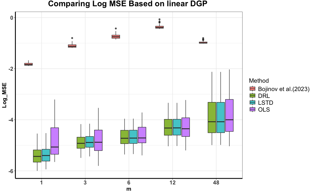
In this section, we design two simulation environments sharing a common time horizon $T=48$ and state dimension $d=3$: one with a linear data generating process (DGP) and the other with a nonlinear DGP, to evaluate the performance of various switchback designs and different ATE estimators.

4.1 Environment I: Linear DGP

Data is generated based on model (3). The number of days $n$ used in our simulations varies, selected from the set $\{16,20,24,28,32,36,40,44,48,52\}$. The initial state for each day is drawn from a 3-dimensional multivariate normal distribution with zero mean and an identity covariance matrix. The coefficients for these models are specified as : $\{\gamma_{t}\}_{t}\stackrel{{\scriptstyle i.i.d.}}{{\sim}}U[0.5,0.8],\quad\{\Gamma_{t}^{(j)}\}_{t,j}\stackrel{{\scriptstyle i.i.d.}}{{\sim}}N(0,0.3^{2}),\quad\{\Phi_{t}^{(j_{1},j_{2})}\}_{t,j_{1},j_{2}}\stackrel{{\scriptstyle i.i.d.}}{{\sim}}U[-0.3,0.3]$ and

$$\begin{split}&\{\alpha_{t}\}_{t}\stackrel{{\scriptstyle i.i.d.}}{{\sim}}\begin{cases}U[-1,-0.5]&\text{ with probability 0.5 }\\ U[0.5,1]&\text{ with probability 0.5 }\end{cases},\{\beta_{t}^{(j)}\}_{t,j}\stackrel{{\scriptstyle i.i.d.}}{{\sim}}\begin{cases}U[0.1,0.3]&\text{ with probability 0.5 }\\ U[0.5,1]&\text{ with probability 0.5 }\end{cases},\\ &\{\phi_{t}^{(j)}\}_{t,j}\stackrel{{\scriptstyle i.i.d.}}{{\sim}}\begin{cases}U[-1,-0.5]&\text{ with probability 0.5 }\\ U[0.5,1]&\text{ with probability 0.5 }\end{cases}.\end{split}$$

Here, the superscript $j$ denotes the $j$th component of each vector, while $(j_{1},j_{2})$ indicates the element in the $j_{1}$th row and $j_{2}$th column of each matrix.

Both the reward error $e_{t}$ and the residual in the state regression model $E_{t}=S_{t+1}-{\mathbb{E}}(S_{t+1}|A_{t},S_{t})$ are set to mean zero Gaussian noises. Specifically, $e_{t}=\eta_{t}+\varepsilon_{t}$ where $\{\varepsilon_{t}\}_{t}$ are i.i.d. Gaussian errors $N(0,1.5)$, and $\{\eta_{t}\}_{t}$ are random effects with an autoregressive covariance function: $\sigma_{\eta}(t_{1},t_{2})=1.5\rho_{0}^{|t_{1}-t_{2}|}$. The parameter $\rho_{0}$ is varied among the set $\{0.3,0.5,0.7,0.9\}$. The sequence $\{E_{t}\}_{t}$ is set to an i.i.d. multivariate Gaussian error process, with a covariance matrix 1.5 times the identity matrix, and it is independent of $\{e_{t}\}_{t}$.

Estimation. We employ OLS, LSTD and DRL to estimate ATEs under various designs. For the LSTD, we adapt the algorithm detailed in Section 3.2.2 by including the time index within the state and aggregating data across time points during each iteration. This modification is designed to borrow information over time, thereby improving the accuracy of the estimated value function. A similar strategy is employed by Bian et al. (2023) to effectively utilize data across time and populations in doubly inhomogeneous environments. To implement the DRL, we compute the value function using the modified LSTD algorithm and develop model-based methods to estimate the marginalized IS ratio. An in-depth discussion on the estimation of this ratio and the modified LSTD algorithm can be found in Section A of the supplementary article.
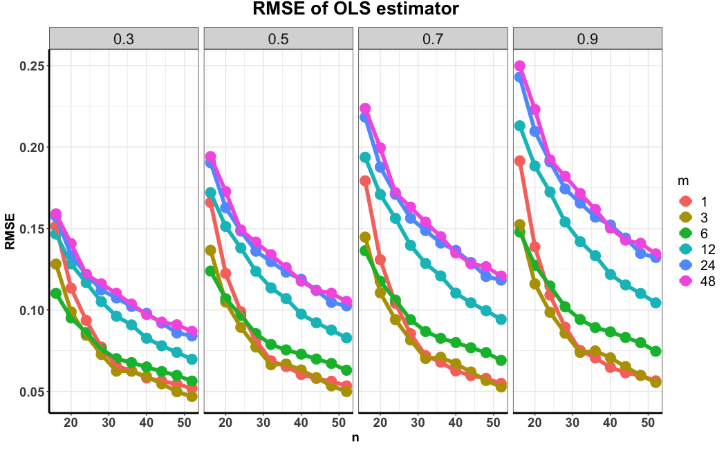
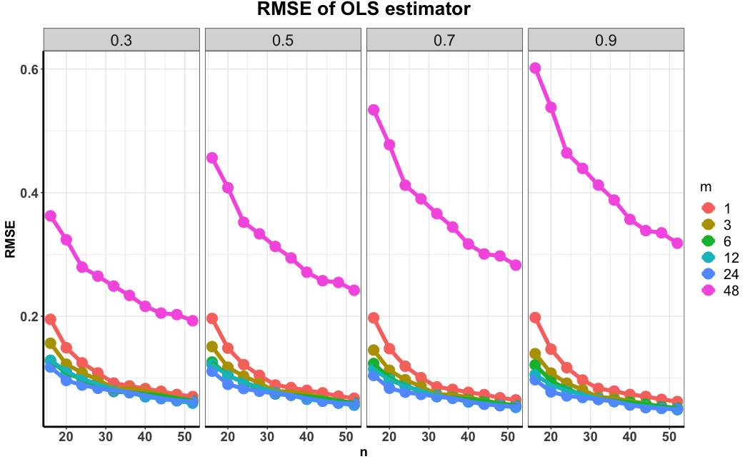
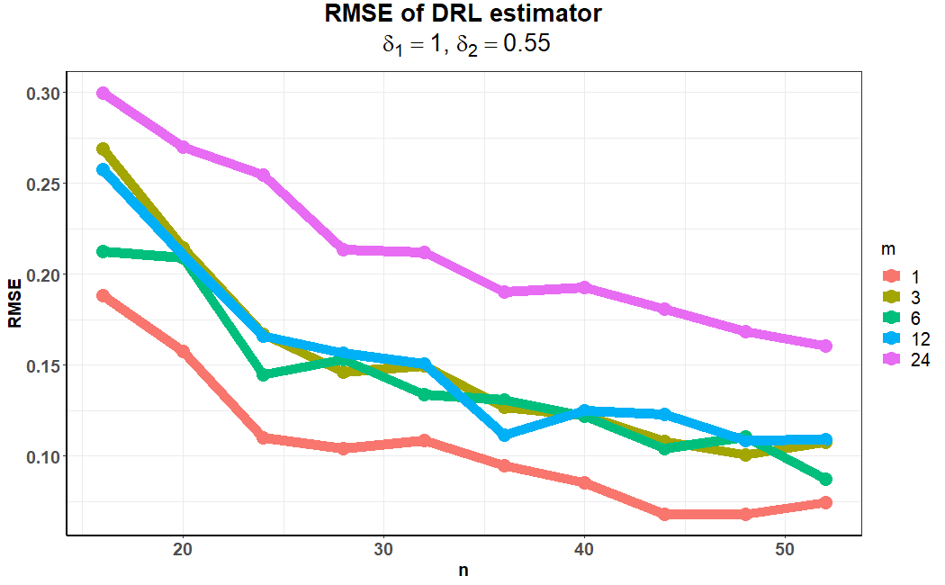
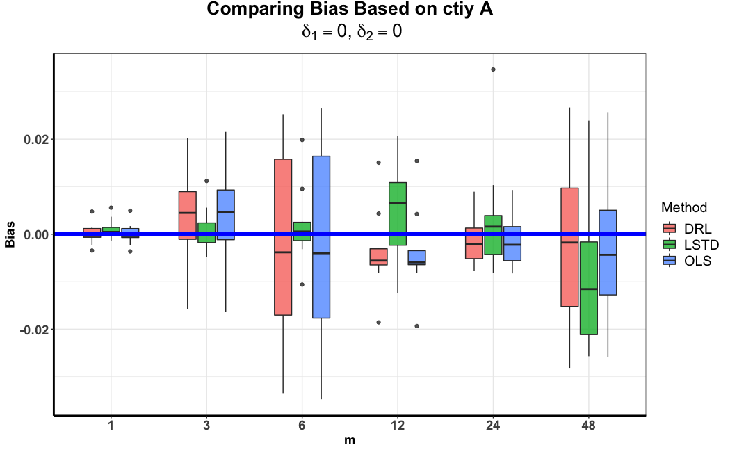
Refer to caption
Refer to caption
Refer to caption
Refer to caption
Refer to caption
Refer to caption
Figure 4: Simulation results with different combinations of $(n,m,\rho_{0})$ alongside different estimation procedures. The left panels report the root MSEs (RMSEs) of ATE estimators under Environment I – the linear DGP. The right panels report the RMSEs of ATE estimators under Environment II – the nonlinear DGP. The ATE estimators are computed based on OLS, LSTD and DRL, from top to bottom.

Results. We implement various $m$-switchback designs with $m\in\{1,3,6,12,24,48\}$ in this environment and report the root MSEs of the resulting ATE estimators aggregated over 200 simulations in the left panels of Figure 4, considering different combinations of $n$, $\rho_{0}$ and the estimating procedure. Notably, when $m=48$, the resulting design coincides with the alternating-day design. It can be seen from Figure 4 that the RMSE decays with $m$ in most cases, which empirically validate our theoretical findings. Additionally, the difference in RMSE between the switchback design and the alternating-day design grows with $\rho_{0}$, which corresponds to the auto-correlation coefficient of $\{e_{t}\}_{t}$. This aligns with our analysis, suggesting that a higher degree of positive correlation in the residuals favors the switchback design over the alternating-day design. We further visualize the biases and standard deviations of these ATE estimators in Figure 11; see the Section A of the supplementary article. These analyses indicate that ATE estimators under different switchback designs exhibit minimal and comparable biases, while their standard deviations clearly increase with $m$.

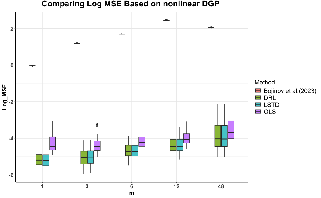
4.2 Experiment II: Nonlinear DGP

We consider the nonlinear reward function: $r_{t}(a,s)=\alpha_{t}+2\beta_{t}^{\top}[\sin(sa)+\cos(s)]^{2}+3(\beta_{t}^{\top}s)\gamma_{t}a+[a\gamma_{t}+\cos(a\gamma_{t})]^{2}$, where the sine, cosine, and square functions are applied element-wise to each component of the vector. The state regression function remains linear and identical to the one presented in (3). All model parameters, including $\{\alpha_{t}\}_{t}$, $\{\beta_{t}\}_{t}$, $\{\gamma_{t}\}_{t}$, $\{\Gamma_{t}\}_{t}$, $\{\phi_{t}\}_{t}$, $n$ and $T$, are the same as those in Section 4.1, with the exception of $\Phi_{t}^{(j_{1},j_{2})}\stackrel{{\scriptstyle i.i.d.}}{{\sim}}U[-0.6,0.6]$ for $j_{1},j_{2}=1,2,3$.

Estimation. The estimation procedure is identical to the one presented in (3).

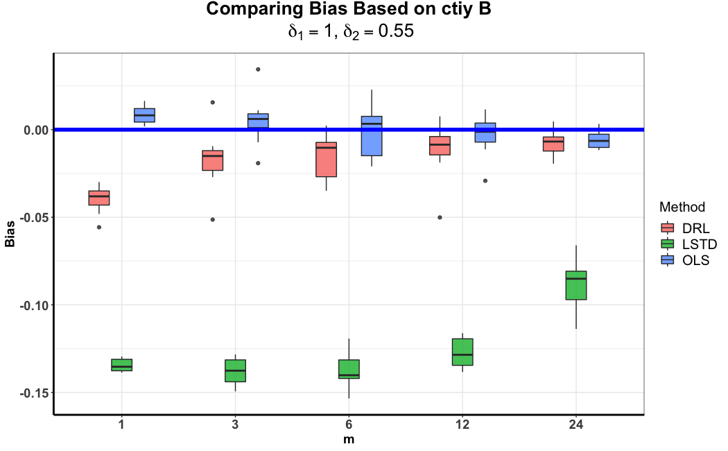
Results. We similarly implement different $m$-switchback designs with $m\in\{1,3,6,12,24,48\}$ and report the RMSEs of the resulting estimators in the right panels of Figure 4. The results closely resemble those observed in Section 4.1. Specifically, the RMSE generally decreases with $m$ and increases with $\rho_{0}$, providing empirical evidence in favor of more frequent switching in switchback designs. For additional details, including biases and standard deviations of the estimators, refer to Figure 12 in the supplementary material. It is worth noting that the OLS-based ATE estimators exhibit larger absolute bias than the LSTD- and DRL-based estimators, primarily due to the misspecification of the linear model.

Refer to caption
Refer to caption
Refer to caption
Refer to caption
Figure 5: Numerical results for the linear DGP: RMSEs of OLS estimator with different combinations of $(n,m,\rho_{0})$ alongside four covariance structures: moving average (top left), exchangeable with a positive correlation (top right), autoregressive with a negative autocorrelation (bottom left) and uncorrelated (bottom right).

4.3 Experiment III: Sensitivity of Covariance Structure

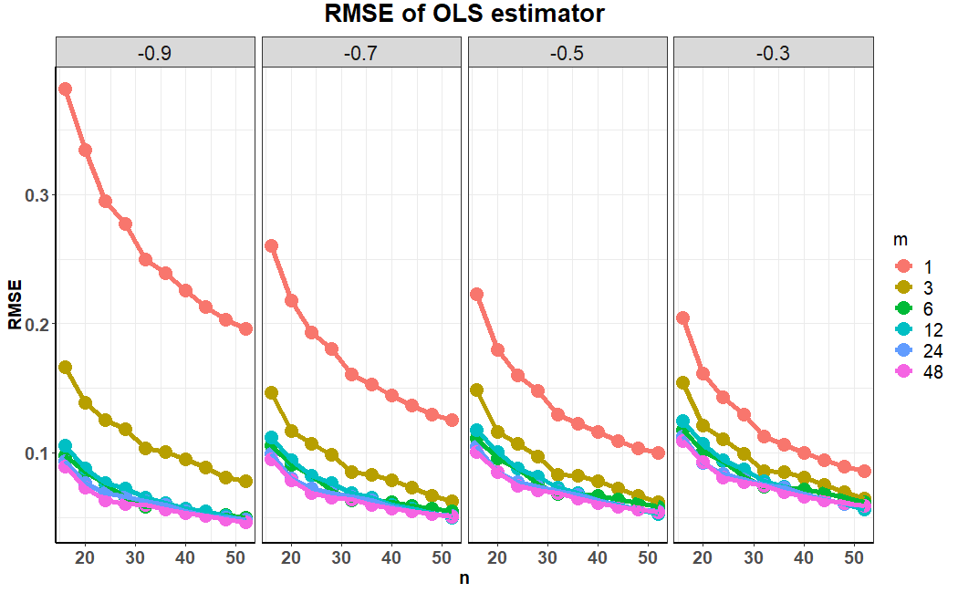
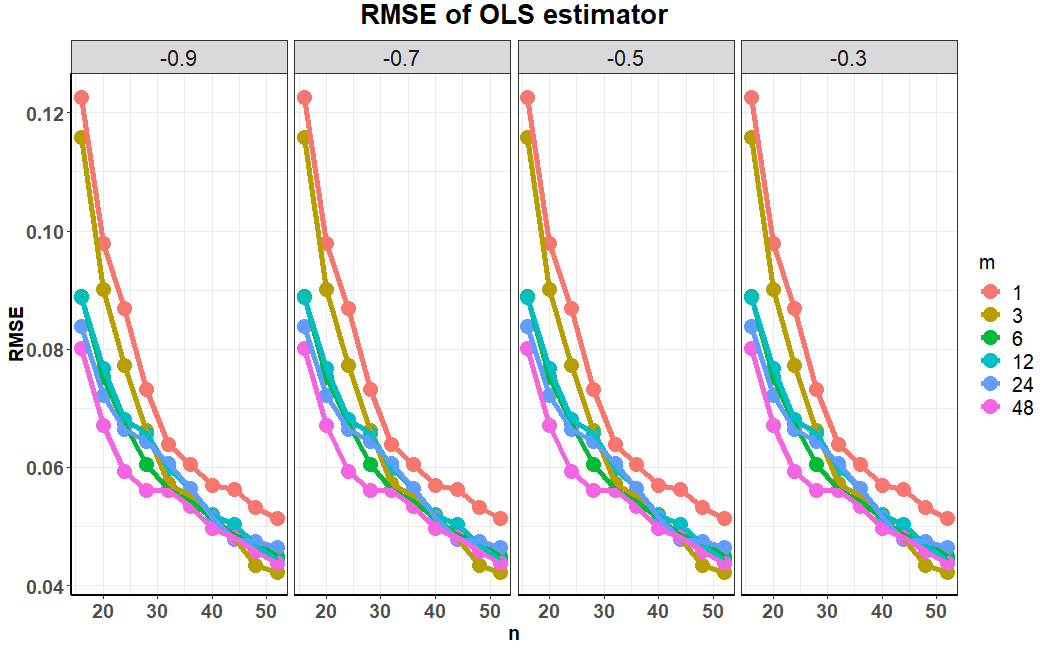
In the first two experiments, the reward errors follow an autoregressive covariance structure with a positive autocorrelation. In this experiment, we consider four additional covariance structures: moving average, exchangeable (with a positive correlation), autoregressive (with a negative autocorrelation) and uncorrelated. We focus on OLS estimators and report their MSEs under different designs in Figure 5 and Figure 13 (refer to Section A of the supplementary article). it is evident that the efficiency of switchback designs either increases or decreases with $m$, depending on the presence of negative or positive correlation. In the case of uncorrelated errors, most designs exhibit similar performance levels. These results align with our theoretical findings.

4.4 Experiment IV: Comparison

We further compare our ATE estimators against those under the regular switchback design proposed by Bojinov et al. (2023). While similar in relying on a hyperparameter $m$ that determines the duration of each policy switch, their design differs in that after applying a treatment for $m$ time intervals, there is a 50% probability of continuing with the same treatment or switching to the other (see Definition 1 in Section A of the supplementary article). They employ multi-step importance sampling to construct the ATE estimator and find that the optimal choice of $m$ is determined by the duration of the carryover effect, which equals $\infty$ under the MDP. We report the log(MSEs) of various ATEs under different designs in Figure 6, with different choices of $m$. It clearly shows our ATEs’ superiority over those used in their designs. More details can be found in Section A of the supplementary article.

Refer to caption
Refer to caption
Figure 6: Boxplots depicting log rmses of all ATE estimators for various combinations of $m$ under the linear DGP (left) and nonlinear DGP (right).

5 Real Data-based Simulation

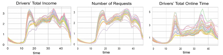
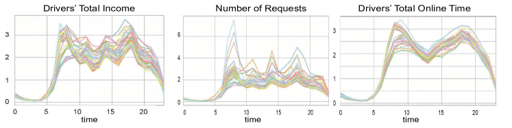
We conduct the analysis based on two real datasets obtained from a world-leading ridesharing company. The first dataset covers the period from Dec. 5th, 2018, to Jan. 13th, 2019, with thirty minutes defined as one time unit, resulting in $T=48$. The second dataset spans from May 17th, 2019, to June 25th, 2019, with one-hour time units, leading to $T=24$. Both datasets contain 40 days of data (i.e., $N=40$). For privacy reasons, we do not disclose the company’s name or the cities involved. Additionally, all metrics (e.g., states and rewards) presented in this paper are scaled to ensure privacy.

The state variable consists of the number of order requests and the driver’s total online time within each 30-minute or one-hour time interval. These variables measure the demand and supply dynamics of the ridesharing platform and have significant impact on the platform’s outcomes (Shi et al., 2023). The reward is the total income earned by the drivers within each time interval, whose residual shows a noticeable positive correlation, as depicted in Figure 1. Figure 7 (see the Section A of the supplementary article) plots these three variables, revealing seasonable temporal trends within each day, with peaks during peak hours. This observation justifies the use of a time-varying MDP model, as described in Section 2.

Refer to caption
Refer to caption
Figure 7: Visual representations of scaled states and rewards in two cities across 40 days, comprising drivers’ total income, the numbers of requests and drivers’ total online time. Each row represents data from a different city.
Refer to caption
Refer to caption
Refer to caption
Refer to caption
Refer to caption
Refer to caption
Refer to caption
Refer to caption
Refer to caption
Figure 8: Empirical results for the first city: RMSEs of ATE estimators with different combinations of $n$, $m$, effect sizes, alongside different estimation procedures. The ATE estimators were computed based on OLS, LSTD and DRL, from left panels to right panels. The treatment effect ratio equals 00, $2\%$ and $5\%$, from top panels to bottom panels.
Refer to caption
Refer to caption
Refer to caption
Refer to caption
Refer to caption
Refer to caption
Refer to caption
Refer to caption
Refer to caption
Figure 9: Empirical results for the second city: RMSEs of ATE estimators with different combinations of $n$, $m$, effect sizes, alongside different estimation procedures. The ATE estimators were computed based on OLS, LSTD and DRL, from left panels to right panels. The treatment effect ratio equals 00, $2\%$ and $5\%$, from top panels to bottom panels.

Bootstrap-based simulation. Both datasets are collected from A/A experiments, in which a single order dispatch policy was consistently applied over time ($A_{t}=0$ for all $t$). To utilize these datasets for evaluating the performance of different designs, we create two simulation environments using the wild bootstrap (Wu et al., 1986). A summary of the bootstrap-assisted procedure is provided in Algorithm 5 (see Section A of the supplementary article).

Specifically, for each dataset, we first fit the data based on the linear models in (3). We apply ridge regression to estimate the regression coefficients with the regularization parameter determined by minimizing the generalized cross-validation criterion (Wahba, 1975). This yields the estimators $\{\widehat{\alpha}_{t}\}_{t}$, $\{\widehat{\beta}_{t}\}_{t}$, $\{\widehat{\phi}_{t}\}_{t}$ and $\{\widehat{\Phi}_{t}\}_{t}$. However, $\{\gamma_{t}\}_{t}$ and $\{\Gamma_{t}\}_{t}$ remain unidentifiable, since $A_{t}=0$ almost surely. We then calculate the residuals in the reward and state regression models based on these estimators as follows:

$$\widehat{e}_{i,t}=R_{i,t}-\widehat{\alpha}_{t}-S_{i,t}^{\top}\widehat{\beta}_{t},\quad\widehat{E}_{i,t}=S_{i,t+1}-\widehat{\phi}_{t}-\widehat{\Phi}_{t}S_{i,t}.$$ (13)

To generate simulation data with varying sizes of treatment effect, we introduce the treatment effect ratio parameter $\lambda$ and manually set the treatment effect parameters $\widehat{\gamma}_{t}=\delta_{1}\times(\sum_{i}R_{i,t}/(100\times N))$ and $\widehat{\Gamma}_{t}=\delta_{2}\times(\sum_{i}S_{i,t}/(100\times N))$. The treatment effect ratio essentially corresponds to the ratio of the ATE and the baseline policy’s average return. We consider three choices of $\lambda$, corresponding to 00 (i.e., no treatment effect at all), $2\%$, and $5\%$. For each choice of $\lambda$, $\delta_{1}$ and $\delta_{2}$ are selected such that both the resulting direct effect and carryover effect (see Equation (4)) increase by $\lambda/2$, leading to an overall ATE increase of $\lambda$.

Finally, to create a dataset spanning $n$ days, actions are generated according to the chosen design as described in Section 2. We then sample i.i.d. standard Gaussian noises $\{\xi_{i}\}_{i=1}^{n}$. For the $i$-th day, we uniformly sample an integer $I\in\{1,\dots,N\}$, set the initial state to $S_{I,1}$, and generate rewards and states according to (3) with the estimated $\{\widehat{\alpha}_{t}\}_{t}$, $\{\widehat{\beta}_{t}\}_{t}$, $\{\widehat{\phi}_{t}\}_{t}$, $\{\widehat{\Phi}_{t}\}_{t}$, the specified $\{\widehat{\gamma}_{t}\}_{t}$ and $\{\widehat{\Gamma}_{t}\}_{t}$, and the error residuals given by $\{\xi_{i}\widehat{e}_{i,t}:1\leq t\leq T\}$ and $\{\xi_{i}\widehat{E}_{i,t}:1\leq t\leq T\}$, respectively. This ensures that the error covariance structure of the simulated data closely resembles that of the real datasets. Based on the simulated data, we similarly apply OLS, LSTD and DRL to estimate the ATE and compare their MSEs under various switchback designs.

Refer to caption
Figure 10: The graphical visualization of our proposed workflow guideline. $\text{SB}^{(m)}$ denotes the $m-$switchback design and AD denotes the alternating-day design.

Results: Figures 8 and 9 summarize the results, which strongly support the advantages of employing switchback designs with more frequent switches, especially when there is no or only a minor effect enhancement (i.e., 0 or 2% increase). In the first environment, when the effect sizes increase to 5% and the sample size exceeds 35, the LSTD estimators under different designs achieve comparable MSEs. However, a closer examination of the biases and standard deviations of these ATE estimators (see Figures 14 and 15 in Section A of the supplementary article) reveals that this is mainly due to the large biases of the LSTD estimators. Since these biases are caused by model misspecification, they remain roughly constant under different designs.

6 Discussion

This paper studies switchback designs in the framework of RL. To offer practical guidance, we outline a workflow in this section (see also Figure 10):

  1. (i)

    The first step is to discretize the data to define appropriate time intervals, ensuring that both the state and reward follow the Markov assumption (see (1) and (2)). This can be tested via existing state-of-the-art methods (see e.g., Chen and Hong, 2012; Shi et al., 2020; Zhou et al., 2023). When the Markov assumption is violated, it is necessary to increase the length of time intervals accordingly to satisfy this condition.

  2. (ii)

    The second step is to assess the weak signal condition. Should the signal be strong, the alternating-day (AD) design is recommended. In our numerical studies (not reported in this paper), we observe that with a large treatment effect, the switchback design suffers from larger bias than the AD design.

  3. (iii)

    Finally, if the weak signal condition is verified, we proceed to analyze error correlations. When errors exhibit positive correlations, we recommend to employ the switchback design with $m=1$. In cases where errors are uncorrelated, both the AD design and switchback design demonstrate comparable performance, affording flexibility in selection. However, when errors display negative correlations, the AD design would be preferred.

References

  • Athey et al. (2023) Athey, S., P. J. Bickel, A. Chen, G. W. Imbens, and M. Pollmann (2023). Semi-parametric estimation of treatment effects in randomised experiments. Journal of the Royal Statistical Society Series B: Statistical Methodology 85(5), 1615–1638.
  • Athey and Imbens (2017) Athey, S. and G. W. Imbens (2017). The state of applied econometrics: Causality and policy evaluation. Journal of Economic perspectives 31(2), 3–32.
  • Atkinson and Pedrosa (2017) Atkinson, A. and D. Pedrosa (2017). Optimum design and sequential treatment allocation in an experiment in deep brain stimulation with sets of treatment combinations. Statistics in Medicine 36(30), 4804–4815.
  • Atkinson and Biswas (2013) Atkinson, A. C. and A. Biswas (2013). Randomised response-adaptive designs in clinical trials. Monographs Stat. Appl. Probability 130, 130.
  • Bajari et al. (2021) Bajari, P., B. Burdick, G. W. Imbens, L. Masoero, J. McQueen, T. Richardson, and I. M. Rosen (2021). Multiple randomization designs. arXiv preprint arXiv:2112.13495.
  • Baldi Antognini and Zagoraiou (2011) Baldi Antognini, A. and M. Zagoraiou (2011). The covariate-adaptive biased coin design for balancing clinical trials in the presence of prognostic factors. Biometrika 98(3), 519–535.
  • Begg and Iglewicz (1980) Begg, C. B. and B. Iglewicz (1980). A treatment allocation procedure for sequential clinical trials. Biometrics, 81–90.
  • Bian et al. (2023) Bian, Z., C. Shi, Z. Qi, and L. Wang (2023). Off-policy evaluation in doubly inhomogeneous environments. arXiv preprint arXiv:2306.08719.
  • Bibaut et al. (2019) Bibaut, A., I. Malenica, N. Vlassis, and M. Van Der Laan (2019). More efficient off-policy evaluation through regularized targeted learning. In International Conference on Machine Learning, pp. 654–663. PMLR.
  • Bickel et al. (1993) Bickel, P. J., C. A. Klaassen, P. J. Bickel, Y. Ritov, J. Klaassen, J. A. Wellner, and Y. Ritov (1993). Efficient and adaptive estimation for semiparametric models, Volume 4. Springer.
  • Bojinov and Shephard (2019) Bojinov, I. and N. Shephard (2019). Time series experiments and causal estimands: exact randomization tests and trading. Journal of the American Statistical Association 114(528), 1665–1682.
  • Bojinov et al. (2023) Bojinov, I., D. Simchi-Levi, and J. Zhao (2023). Design and analysis of switchback experiments. Management Science 69(7), 3759–3777.
  • Bradtke and Barto (1996) Bradtke, S. J. and A. G. Barto (1996). Linear least-squares algorithms for temporal difference learning. Machine learning 22, 33–57.
  • Chen and Hong (2012) Chen, B. and Y. Hong (2012). Testing for the markov property in time series. Econometric Theory 28(1), 130–178.
  • Chen et al. (2016) Chen, G., D. Zeng, and M. R. Kosorok (2016). Personalized dose finding using outcome weighted learning. Journal of the American Statistical Association 111(516), 1509–1521.
  • Chen and Jiang (2019) Chen, J. and N. Jiang (2019). Information-theoretic considerations in batch reinforcement learning. In International Conference on Machine Learning, pp. 1042–1051. PMLR.
  • Chen and Christensen (2015) Chen, X. and T. M. Christensen (2015). Optimal uniform convergence rates and asymptotic normality for series estimators under weak dependence and weak conditions. Journal of Econometrics 188(2), 447–465.
  • Chen and Qi (2022) Chen, X. and Z. Qi (2022). On well-posedness and minimax optimal rates of nonparametric q-function estimation in off-policy evaluation. In International Conference on Machine Learning, pp. 3558–3582. PMLR.
  • Chernozhukov et al. (2018) Chernozhukov, V., D. Chetverikov, M. Demirer, E. Duflo, C. Hansen, W. Newey, and J. Robins (2018). Double/debiased machine learning for treatment and structural parameters.  21(1), C1–C68.
  • Chernozhukov et al. (2022) Chernozhukov, V., W. Newey, R. Singh, and V. Syrgkanis (2022). Automatic debiased machine learning for dynamic treatment effects and general nested functionals. arXiv preprint arXiv:2203.13887.
  • Ertefaie and Strawderman (2018) Ertefaie, A. and R. L. Strawderman (2018). Constructing dynamic treatment regimes over indefinite time horizons. Biometrika 105(4), 963–977.
  • Fan et al. (2020) Fan, J., Z. Wang, Y. Xie, and Z. Yang (2020). A theoretical analysis of deep q-learning. In Learning for dynamics and control, pp.  486–489. PMLR.
  • Farias et al. (2022) Farias, V., A. Li, T. Peng, and A. Zheng (2022). Markovian interference in experiments. Advances in Neural Information Processing Systems 35, 535–549.
  • Gottesman et al. (2019) Gottesman, O., Y. Liu, S. Sussex, E. Brunskill, and F. Doshi-Velez (2019). Combining parametric and nonparametric models for off-policy evaluation. In International Conference on Machine Learning, pp. 2366–2375. PMLR.
  • Grenander (1981) Grenander, U. (1981). Abstract inference. Wiley Series, New York.
  • Hanna et al. (2019) Hanna, J., S. Niekum, and P. Stone (2019). Importance sampling policy evaluation with an estimated behavior policy. In International Conference on Machine Learning, pp. 2605–2613. PMLR.
  • Hanna et al. (2017) Hanna, J. P., P. S. Thomas, P. Stone, and S. Niekum (2017). Data-efficient policy evaluation through behavior policy search. In International Conference on Machine Learning, pp. 1394–1403. PMLR.
  • Hao et al. (2021) Hao, B., X. Ji, Y. Duan, H. Lu, C. Szepesvari, and M. Wang (2021). Bootstrapping fitted q-evaluation for off-policy inference. In International Conference on Machine Learning, pp. 4074–4084. PMLR.
  • Hu et al. (2009) Hu, F., L.-X. Zhang, and X. He (2009). Efficient randomized-adaptive designs. The Annals of Statistics, 2543–2560.
  • Hu et al. (2015) Hu, J., H. Zhu, and F. Hu (2015). A unified family of covariate-adjusted response-adaptive designs based on efficiency and ethics. Journal of the American Statistical Association 110(509), 357–367.
  • Hu and Wager (2022) Hu, Y. and S. Wager (2022). Switchback experiments under geometric mixing. arXiv preprint arXiv:2209.00197.
  • Hu and Wager (2023) Hu, Y. and S. Wager (2023). Off-policy evaluation in partially observed markov decision processes under sequential ignorability. The Annals of Statistics 51(4), 1561–1585.
  • Huang (1998) Huang, J. Z. (1998). Projection estimation in multiple regression with application to functional anova models. The annals of statistics 26(1), 242–272.
  • Hudgens and Halloran (2008) Hudgens, M. G. and M. E. Halloran (2008). Toward causal inference with interference. Journal of the American Statistical Association 103(482), 832–842.
  • Jiang and Li (2016) Jiang, N. and L. Li (2016). Doubly robust off-policy value evaluation for reinforcement learning. In International Conference on Machine Learning, pp. 652–661. PMLR.
  • Jin et al. (2020) Jin, C., Z. Yang, Z. Wang, and M. I. Jordan (2020). Provably efficient reinforcement learning with linear function approximation. In Conference on Learning Theory, pp.  2137–2143. PMLR.
  • Johari et al. (2017) Johari, R., P. Koomen, L. Pekelis, and D. Walsh (2017). Peeking at a/b tests: Why it matters, and what to do about it. In Proceedings of the 23rd ACM SIGKDD International Conference on Knowledge Discovery and Data Mining, pp.  1517–1525.
  • Johari et al. (2022) Johari, R., H. Li, I. Liskovich, and G. Y. Weintraub (2022). Experimental design in two-sided platforms: An analysis of bias. Management Science 68(10), 7065–7791.
  • Jones and Goos (2009) Jones, B. and P. Goos (2009). D-optimal design of split-split-plot experiments. Biometrika 96(1), 67–82.
  • Kallus and Uehara (2022) Kallus, N. and M. Uehara (2022). Efficiently breaking the curse of horizon in off-policy evaluation with double reinforcement learning. Operations Research 70(6), 3282–3302.
  • Kong et al. (2021) Kong, X., M. Yuan, and W. Zheng (2021). Approximate and exact designs for total effects. The Annals of Statistics 49(3), 1594–1625.
  • Krishnamurthy (2016) Krishnamurthy, V. (2016). Partially observed Markov decision processes. Cambridge university press.
  • Larsen et al. (2023) Larsen, N., J. Stallrich, S. Sengupta, A. Deng, R. Kohavi, and N. T. Stevens (2023). Statistical challenges in online controlled experiments: A review of a/b testing methodology. The American Statistician (just-accepted), 1–32.
  • Leung (2022) Leung, M. P. (2022). Rate-optimal cluster-randomized designs for spatial interference. The Annals of Statistics 50(5), 3064–3087.
  • Li et al. (2021) Li, G., Y. Chen, Y. Chi, Y. Gu, and Y. Wei (2021). Sample-efficient reinforcement learning is feasible for linearly realizable mdps with limited revisiting. Advances in Neural Information Processing Systems 34, 16671–16685.
  • Li et al. (2023) Li, G., W. Wu, Y. Chi, C. Ma, A. Rinaldo, and Y. Wei (2023). Sharp high-probability sample complexities for policy evaluation with linear function approximation. arXiv preprint arXiv:2305.19001.
  • Li et al. (2024) Li, T., C. Shi, Z. Lu, Y. Li, and H. Zhu (2024). Evaluating dynamic conditional quantile treatment effects with applications in ridesharing. Journal of the American Statistical Association (just-accepted), 1–26.
  • Li et al. (2023) Li, T., C. Shi, J. Wang, F. Zhou, et al. (2023). Optimal treatment allocation for efficient policy evaluation in sequential decision making. Advances in Neural Information Processing Systems 36.
  • Li et al. (2019) Li, X., P. Ding, Q. Lin, D. Yang, and J. S. Liu (2019). Randomization inference for peer effects. Journal of the American Statistical Association 114(528), 1651–1664.
  • Liao et al. (2021) Liao, P., P. Klasnja, and S. Murphy (2021). Off-policy estimation of long-term average outcomes with applications to mobile health. Journal of the American Statistical Association 116(533), 382–391.
  • Liao et al. (2022) Liao, P., Z. Qi, R. Wan, P. Klasnja, and S. A. Murphy (2022). Batch policy learning in average reward markov decision processes. Annals of statistics 50(6), 3364.
  • Liu et al. (2018) Liu, Q., L. Li, Z. Tang, and D. Zhou (2018). Breaking the curse of horizon: Infinite-horizon off-policy estimation. In Advances in Neural Information Processing Systems, pp. 5356–5366.
  • Liu et al. (2023) Liu, W., J. Tu, Y. Zhang, and X. Chen (2023). Online estimation and inference for robust policy evaluation in reinforcement learning. arXiv preprint arXiv:2310.02581.
  • Luckett et al. (2019) Luckett, D. J., E. B. Laber, A. R. Kahkoska, D. M. Maahs, E. Mayer-Davis, and M. R. Kosorok (2019). Estimating dynamic treatment regimes in mobile health using V-learning. Journal of the American Statistical Association accepted.
  • Luo et al. (2024) Luo, S., Y. Yang, C. Shi, F. Yao, J. Ye, and H. Zhu (2024). Policy evaluation for temporal and/or spatial dependent experiments. Journal of the Royal Statistical Society Series B: Statistical Methodology, 1–27.
  • Mukherjee et al. (2022) Mukherjee, S., J. P. Hanna, and R. D. Nowak (2022). Revar: Strengthening policy evaluation via reduced variance sampling. In Uncertainty in Artificial Intelligence, pp.  1413–1422. PMLR.
  • Newey et al. (1998) Newey, W. K., F. Hsieh, and J. Robins (1998). Undersmoothing and bias corrected functional estimation.
  • Ni et al. (2023) Ni, T., I. Bojinov, and J. Zhao (2023). Design of panel experiments with spatial and temporal interference. Available at SSRN 4466598.
  • Puterman (2014) Puterman, M. L. (2014). Markov decision processes: discrete stochastic dynamic programming. John Wiley & Sons.
  • Qin et al. (2022) Qin, Z. T., H. Zhu, and J. Ye (2022). Reinforcement learning for ridesharing: An extended survey. Transportation Research Part C: Emerging Technologies 144, 103852.
  • Quin et al. (2024) Quin, F., D. Weyns, M. Galster, and C. C. Silva (2024). A/b testing: a systematic literature review. Journal of Systems and Software, 112011.
  • Reich et al. (2021) Reich, B. J., S. Yang, Y. Guan, A. B. Giffin, M. J. Miller, and A. Rappold (2021). A review of spatial causal inference methods for environmental and epidemiological applications. International Statistical Review 89(3), 605–634.
  • Robins (1986) Robins, J. (1986). A new approach to causal inference in mortality studies with a sustained exposure period—application to control of the healthy worker survivor effect. Mathematical modelling 7(9-12), 1393–1512.
  • Rosenblum et al. (2020) Rosenblum, M., E. X. Fang, and H. Liu (2020). Optimal, two-stage, adaptive enrichment designs for randomized trials, using sparse linear programming. Journal of the Royal Statistical Society Series B: Statistical Methodology 82(3), 749–772.
  • Rubin (2005) Rubin, D. B. (2005). Causal inference using potential outcomes: Design, modeling, decisions. Journal of the American Statistical Association 100(469), 322–331.
  • Shen (1997) Shen, X. (1997). On methods of sieves and penalization. The Annals of Statistics 25(6), 2555–2591.
  • Shi et al. (2023) Shi, C., Z. Qi, J. Wang, and F. Zhou (2023). Value enhancement of reinforcement learning via efficient and robust trust region optimization. Journal of the American Statistical Association accepted.
  • Shi et al. (2021) Shi, C., R. Wan, V. Chernozhukov, and R. Song (2021). Deeply-debiased off-policy interval estimation. In International conference on machine learning, pp. 9580–9591. PMLR.
  • Shi et al. (2020) Shi, C., R. Wan, R. Song, W. Lu, and L. Leng (2020). Does the markov decision process fit the data: Testing for the markov property in sequential decision making. In International Conference on Machine Learning, pp. 8807–8817. PMLR.
  • Shi et al. (2023) Shi, C., X. Wang, S. Luo, H. Zhu, J. Ye, and R. Song (2023). Dynamic causal effects evaluation in a/b testing with a reinforcement learning framework. Journal of the American Statistical Association 118(543), 2059–2071.
  • Shi et al. (2022) Shi, C., S. Zhang, W. Lu, and R. Song (2022). Statistical inference of the value function for reinforcement learning in infinite-horizon settings. Journal of the Royal Statistical Society Series B: Statistical Methodology 84(3), 765–793.
  • Stone (1982) Stone, C. J. (1982). Optimal global rates of convergence for nonparametric regression. The annals of statistics, 1040–1053.
  • Sutton and Barto (2018) Sutton, R. S. and A. G. Barto (2018). Reinforcement learning: An introduction. MIT press.
  • Tang et al. (2019) Tang, X., Z. Qin, F. Zhang, Z. Wang, Z. Xu, Y. Ma, H. Zhu, and J. Ye (2019). A deep value-network based approach for multi-driver order dispatching. In The 25th ACM SIGKDD Conference on Knowledge Discovery and Data Mining (KDD’19) 25, 1780–1790.
  • Tang et al. (2022) Tang, Z., Y. Duan, S. Zhang, and L. Li (2022). A reinforcement learning approach to estimating long-term treatment effects. arXiv preprint arXiv:2210.07536.
  • Thams et al. (2023) Thams, N., S. Saengkyongam, N. Pfister, and J. Peters (2023). Statistical testing under distributional shifts. Journal of the Royal Statistical Society Series B: Statistical Methodology 85(3), 597–663.
  • Thomas and Brunskill (2016) Thomas, P. and E. Brunskill (2016). Data-efficient off-policy policy evaluation for reinforcement learning. In International Conference on Machine Learning, pp. 2139–2148.
  • Thomas et al. (2015) Thomas, P. S., G. Theocharous, and M. Ghavamzadeh (2015). High-confidence off-policy evaluation. In Twenty-Ninth AAAI Conference on Artificial Intelligence.
  • Tropp (2012) Tropp, J. A. (2012). User-friendly tail bounds for sums of random matrices. Foundations of computational mathematics 12, 389–434.
  • Tsiatis (2007) Tsiatis, A. (2007). Semiparametric Theory and Missing Data. Springer Science & Business Media.
  • Uehara et al. (2020) Uehara, M., J. Huang, and N. Jiang (2020). Minimax weight and q-function learning for off-policy evaluation. In International Conference on Machine Learning, pp. 9659–9668. PMLR.
  • Uehara et al. (2021) Uehara, M., M. Imaizumi, N. Jiang, N. Kallus, W. Sun, and T. Xie (2021). Finite sample analysis of minimax offline reinforcement learning: Completeness, fast rates and first-order efficiency. arXiv preprint arXiv:2102.02981.
  • Uehara et al. (2022) Uehara, M., C. Shi, and N. Kallus (2022). A review of off-policy evaluation in reinforcement learning. arXiv preprint arXiv:2212.06355.
  • Ugander et al. (2013) Ugander, J., B. Karrer, L. Backstrom, and J. Kleinberg (2013). Graph cluster randomization: Network exposure to multiple universes. In Proceedings of the 19th ACM SIGKDD International Conference on Knowledge Discovery and Data Mining, pp.  329–337.
  • Van and Wellner (1996) Van, D. and J. A. Wellner (1996). Weak convergence and empirical processes. Springer,.
  • Viviano and Bradic (2023) Viviano, D. and J. Bradic (2023). Synthetic learner: model-free inference on treatments over time. Journal of Econometrics 234(2), 691–713.
  • Wahba (1975) Wahba, G. (1975). Smoothing noisy data with spline functions. Numerische mathematik 24(5), 383–393.
  • Wan et al. (2022) Wan, R., B. Kveton, and R. Song (2022). Safe exploration for efficient policy evaluation and comparison. In International Conference on Machine Learning, pp. 22491–22511. PMLR.
  • Wan et al. (2023) Wan, R., Y. Liu, J. McQueen, D. Hains, and R. Song (2023). Experimentation platforms meet reinforcement learning: Bayesian sequential decision-making for continuous monitoring. In Proceedings of the 29th ACM SIGKDD Conference on Knowledge Discovery and Data Mining, pp.  5016–5027.
  • Wang et al. (2023) Wang, J., Z. Qi, and R. K. Wong (2023). Projected state-action balancing weights for offline reinforcement learning. The Annals of Statistics 51(4), 1639–1665.
  • Wang et al. (2018) Wang, L., Y. Zhou, R. Song, and B. Sherwood (2018). Quantile-optimal treatment regimes. Journal of the American Statistical Association 113(523), 1243–1254.
  • Wang et al. (2024) Wang, W., Y. Li, and X. Wu (2024). Off-policy evaluation for tabular reinforcement learning with synthetic trajectories. Statistics and Computing 34(1), 41.
  • Waudby-Smith et al. (2022) Waudby-Smith, I., L. Wu, A. Ramdas, N. Karampatziakis, and P. Mineiro (2022). Anytime-valid off-policy inference for contextual bandits. ACM/JMS Journal of Data Science.
  • Wong and Zhu (2008) Wong, W. K. and W. Zhu (2008). Optimum treatment allocation rules under a variance heterogeneity model. Statistics in Medicine 27(22), 4581–4595.
  • Wu et al. (1986) Wu, C.-F. J. et al. (1986). Jackknife, bootstrap and other resampling methods in regression analysis. the Annals of Statistics 14(4), 1261–1295.
  • Xie et al. (2023) Xie, C., W. Yang, and Z. Zhang (2023). Semiparametrically efficient off-policy evaluation in linear markov decision processes. In International Conference on Machine Learning. PMLR.
  • Xiong et al. (2023) Xiong, R., A. Chin, and S. J. Taylor (2023). Data-driven switchback designs: Theoretical tradeoffs and empirical calibration. Available at SSRN.
  • Xu et al. (2018) Xu, Z., Z. Li, Q. Guan, D. Zhang, Q. Li, J. Nan, C. Liu, W. Bian, and J. Ye (2018). Large-scale order dispatch in on-demand ride-hailing platforms: A learning and planning approach. In Proceedings of the 24th ACM SIGKDD International Conference on Knowledge Discovery & Data Mining, KDD ’18, New York, NY, USA, pp. 905–913. Association for Computing Machinery.
  • Yang et al. (2017) Yang, F., A. Ramdas, K. Jamieson, and M. Wainwright (2017). A framework for multi-a (rmed)/b (andit) testing with online fdr control. In Proceedings of the 31st International Conference on Neural Information Processing Systems, pp.  5959–5968.
  • Yin and Wang (2020) Yin, M. and Y.-X. Wang (2020). Asymptotically efficient off-policy evaluation for tabular reinforcement learning. In International Conference on Artificial Intelligence and Statistics, pp.  3948–3958. PMLR.
  • Yu et al. (2021) Yu, C., J. Liu, S. Nemati, and G. Yin (2021). Reinforcement learning in healthcare: A survey. ACM Computing Surveys (CSUR) 55(1), 1–36.
  • Zhang et al. (2013) Zhang, B., A. A. Tsiatis, E. B. Laber, and M. Davidian (2013). Robust estimation of optimal dynamic treatment regimes for sequential treatment decisions. Biometrika 100(3), 681–694.
  • Zhao et al. (2012) Zhao, Y., D. Zeng, A. J. Rush, and M. R. Kosorok (2012). Estimating individualized treatment rules using outcome weighted learning. Journal of the American Statistical Association 107(499), 1106–1118.
  • Zhong et al. (2022) Zhong, R., D. Zhang, L. Schäfer, S. Albrecht, and J. Hanna (2022). Robust on-policy sampling for data-efficient policy evaluation in reinforcement learning. Advances in Neural Information Processing Systems 35, 37376–37388.
  • Zhou et al. (2021) Zhou, F., S. Luo, X. Qie, J. Ye, and H. Zhu (2021). Graph-based equilibrium metrics for dynamic supply–demand systems with applications to ride-sourcing platforms. Journal of the American Statistical Association 116(536), 1688–1699.
  • Zhou et al. (2023) Zhou, Y., Z. Qi, C. Shi, and L. Li (2023). Optimizing pessimism in dynamic treatment regimes: A bayesian learning approach. In International Conference on Artificial Intelligence and Statistics, pp.  6704–6721. PMLR.
  • Zhou et al. (2023) Zhou, Y., C. Shi, L. Li, and Q. Yao (2023). Testing for the markov property in time series via deep conditional generative learning. Journal of the Royal Statistical Society Series B: Statistical Methodology 85(4), 1204–1222.

This appendix is organized as follows. We discuss some implementation details in Section A. Some additional numerical results are reported in Section B. Finally, proofs are provided in Section C.

Appendix A Implementation Details

Modified LSTD. In the original LSTD algorithm described in Section 3.2.2, the value function at a specific time $t$ is estimated using only the data subset corresponding to that particular time. This approach might be inefficient when the system dynamics remain relatively consistent over time. To enhance estimation efficiency, we incorporate the time index into the state, resulting in an augmented state, denoted as $\widetilde{S}_{t}$ for each time $t$. We then approximate the value function using a linear combination of sieves. It is important to note that the basis functions $\varphi$ contains not only the bases for the original state but also those for the time component, addressing potential nonstationarity.

To lay down the foundation, for any $t$, $a$ and $\tilde{s}$, we first define a value function $V_{t:t}^{a}(\tilde{s})={\mathbb{E}}^{a}(R_{t}|\widetilde{S}_{t}=\tilde{s},A_{t}=a)$. Next, we recursively define $V_{t-j:t}^{a}(\tilde{s})={\mathbb{E}}^{a}[R_{t-j}+V_{t-j+1:t}^{a}(\widetilde{S}_{t-j+1})|\widetilde{S}_{t}=\tilde{s},A_{t}=a]$ for $j=1,2,\ldots,t-1$. Essentially, for any $t_{1}\leq t_{2}$, $V_{t_{1}:t_{2}}^{a}$ represents the expected cumulative reward from time $t_{1}$ to $t_{2}$ starting from a given state at time $t_{1}$. Additionally, the final ATE estimator can be represented by ${\mathbb{E}}[V_{1:T}^{1}(\widetilde{S}_{1})-V_{1:T}^{0}(\widetilde{S}_{1})]$.

It remains to estimate these doubly indexed value functions. A key observation is that, with the time index included in the state to account for nonstationarity, $V_{t_{1}:t_{2}}^{a}$ shall equal $V_{t_{3}:t_{4}}^{a}$ provided the time gaps $t_{2}-t_{1}$ and $t_{4}-t_{3}$ are equal. This allows us to aggregate all data over time to simultaneously estimate all value functions.

Our first step is to estimate $\{V_{t:t}^{a}\}_{t}$ by solving the following estimating equation:

$\displaystyle\sum_{i,t}[R_{i,t}-\varphi^{\top}(\widetilde{S}_{i,t})\widehat{\theta}_{0,a}]\varphi(\widetilde{S}_{i,t})\mathbb{I}(A_{i,t}=a)=0.$ (14)

From this, we compute $\widehat{V}_{t:t}^{a}(\tilde{s})$ as $\varphi^{\top}(\tilde{s})\widehat{\theta}_{0,a}$. Next, we sequentially compute $\{V_{t-1:t}^{a}\}_{t}$,$\{V_{t-2:t}^{a}\}_{t}$, and so forth. Specifically, for each $j=1,\ldots,T-1$, we recursively solve the following estimating equation,

$\displaystyle\sum_{i,t}[R_{i,t-j}+\varphi^{\top}(\widetilde{S}_{i,t-j+1})\widehat{\theta}_{j-1,a}-\varphi^{\top}(\widetilde{S}_{i,t-j})\widehat{\theta}_{j,a}]\varphi(\widetilde{S}_{i,t})\mathbb{I}(A_{i,t}=a)=0.$ (15)

This leads to the derivation of $\widehat{\theta}_{j,a}$, based on which we set $\widehat{V}_{t-j:t}^{a}(\tilde{s})$ to $\varphi^{\top}(\tilde{s})\widehat{\theta}_{j,a}$. Finally, we set the ATE estimator to

$\displaystyle\frac{1}{n}\sum_{i=1}^{n}\varphi^{\top}(\widetilde{S}_{i,1})(\widehat{\theta}_{T-1,1}-\widehat{\theta}_{T-1,0}).$ (16)

We provide a pseudocode in Algorithm 3 to summarize the aforementioned procedure.

Data: $\left\{(S_{it},R_{it},A_{it}):1\leq i\leq n,1\leq t\leq T\right\}$.
Result: The ATE estimator
Solve (14) to obtain $\widehat{\theta}_{T,a}$.
for $t=1$ to $T-1$ do
       Solve (15) to obtain $\widehat{\theta}_{T-t,a}$;
end for
Return: The ATE estimator constructed according to (16).
Algorithm 3 Estimating ATE via the modified LSTD.

Estimation of the IS ratios. We have devised a model-based approach to estimate the marginal IS ratio based on the linear model assumption presented in Equation (3). It is worth noting that both the numerator and the denominator of the ratio correspond to the marginal probability density/mass function of the state at a given time, given a sequence of past treatments it has received. As a result, we can focus on estimating these marginal density/mass functions to construct the ratio estimator.

Within the framework of the linear model assumption, we can express the state at time $t$, denoted as $S_{t}$, as follows:

$$S_{t}=\sum_{k=1}^{t-1}\left(\Pi_{l=k+1}^{t-1}\Phi_{l}\right)\phi_{k}+\left(\Pi_{l=1}^{t-1}\Phi_{l}\right)S_{1}+{\sum_{k=1}^{t-1}\left(\Pi_{l=k+1}^{t-1}\Phi_{l}\right)\Gamma_{k}}A_{k}+\sum_{k=1}^{t-1}\left(\Pi_{l=k+1}^{t-1}\Phi_{l}\right)E_{k}.$$ (17)

Consequently, given a sequence of treatments, we can replace $\{A_{k}\}_{k}$ with this treatment sequence to derive the distribution function of $S_{t}$. To estimate this distribution function, we follow these steps:

  1. 1.

    Estimate the model parameters in Equation (3).

  2. 2.

    Impose models for the initial state and the residuals $\{E_{k}\}_{k}$. In our implementation, we utilize normal distributions, and estimate the mean and covariance matrix parameters within these distributions using the available data. According to (17), this ensures that each $S_{t}$ follows a normal distribution as well.

  3. 3.

    Plug the estimated parameters obtained in the first two steps into (17) to construct the mean and covariance matrix estimators for $S_{t}$.

  4. 4.

    Return the normal distribution function with the estimated mean and covariance matrix estimators obtained in Step 3.

A pseudocode summarizing our procedure is presented in Algorithm 4.

Data: $\left\{(S_{it},R_{it},A_{it}):1\leq i\leq n,1\leq t\leq T\right\}$.
Result: The marginal IS ratio estimator.
Initialization: Calculate the least square estimators $\left\{\widehat{\phi}_{t}\right\}_{t=1}^{T-1}$, $\left\{\widehat{\Phi}_{t}\right\}_{t=1}^{T-1}$ and $\left\{\widehat{\Gamma}_{t}\right\}_{t=1}^{T-1}$ in (3);
Impose models for $S_{1}$ and $\{E_{k}\}_{k}$, and estimate the associated model parameters;
for $t=1$ to $T$ do
       1. Derive the probability density/mass function of $S_{t}$ using the aforementioned estimators and (17);
       2. Estimate the numerator $p_{t}^{a}$ by replacing $\{A_{k}\}_{k}$ in Equation (17) with the target policy $a$;
       3. Estimating the denominator $p_{a,t}^{m}$ replacing $\{A_{k}\}_{k}$ in Equation (17) with the treatment sequence under the $m$-switchback design given that $A_{t}=a$;
       4. Calculate the ratio;
      
end for
Algorithm 4 Model-based estimation of the IS ratio.
Input: Real data $\left\{(S_{it},R_{it}):1\leq i\leq n;1\leq t\leq T\right\}$, the adjustment parameters for the ratios $(\delta_{1},\delta_{2})$, $m-$switchback design, the bootstraped samle size $n$, random seed, the bootstrapped size $B$.
Output: The RSMEs, Biases and SDs of different ATE estimators.
Initialization: Calculating the least square estimates $\left\{\widehat{\alpha}\right\}_{t}$, $\left\{\widehat{\beta}_{t}\right\}_{t}$, $\left\{\widehat{\phi}_{t}\right\}_{t}$, $\left\{\widehat{\Phi}_{t}\right\}_{t}$ in the model (3), treatment effect parameters $\left\{\widehat{\gamma}_{t}\right\}_{t}$ and $\left\{\widehat{\Gamma}_{t}\right\}_{t}$ and the residuals of reward model and state regression model by the (13);
for $b=1$ to $B$ do
      
      1. Sampling the number of days $n$ from $\left\{1,\ldots,N\right\}$ with replacement. and generating the i.i.d. normal random variables $\xi_{i}^{b}\sim N(0,1)$;
       2. Generating the pseudo rewards$\left\{\widehat{R}_{i,t}^{b}\right\}_{i,t}$ and states $\left\{\widehat{S}_{i,t}^{b}\right\}_{i,t}$ according to the following equations ,
$$\widehat{R}_{i,t}^{b}=[1,(\widehat{S}_{i,t}^{b})^{\top},A_{i,t}]\begin{pmatrix}\widehat{\alpha}_{t}\\ \widehat{\beta}_{t}\\ \widehat{\gamma}_{t}\end{pmatrix}+\xi_{i}^{b}\widehat{e}_{i,t},\quad\widehat{S}_{i,t+1}^{b}=[\widehat{\phi}_{t},\widehat{\Phi}_{t},\widehat{\Gamma}_{t}]\begin{pmatrix}1\\ \widehat{S}_{i,t}^{b}\\ A_{i,t}\end{pmatrix}+\xi_{i}^{b}\widehat{E}_{i,t}.$$
3. Calculating the set of estimators $\left\{\textrm{ATE}_{\text{SB}}^{(m),b}\right\}_{b,m}$ by OLS, LSTD and DRL.
end for
Algorithm 5 Bootstrap-based simulation.

Estimation of the value function. We devise a model-based approach to estimate the value function. Given the linear models outlined in (3), we can readily express the value function as follows:

$$\begin{split}V_{t}^{a}(s)&=\sum_{j=t}^{T}{\mathbb{E}}^{a}(R_{j}|S_{t}=s)=\sum_{j=t}^{T}[\alpha_{j}+\gamma_{j}a+\beta_{j}^{\top}{\mathbb{E}}^{a}(S_{j}|S_{t}=s)]\\ &=\sum_{j=t}^{T}\Big{\{}\alpha_{j}+\gamma_{j}a+\sum_{j=t}^{T}\beta_{j}^{\top}\Big{[}\sum_{k=t}^{j-1}(\Pi_{l=k+1}^{j-1}\Phi_{l})\phi_{k}+(\Pi_{l=t}^{j-1}\Phi_{l})s+\sum_{k=t}^{j-1}(\Pi_{l=k+1}^{j-1}\Phi_{l})\Gamma_{k}a\Big{]}\Big{\}}\end{split}$$ (18)

This leads us to the approach of initially applying OLS to estimate the model parameters and subsequently incorporating these estimates into (18) to formulate the value function estimators.

Appendix B Additional Simulation Results

Comparison against regular switchback designs. We first introduce the definition of regular switchback designs (Bojinov et al., 2023).

Definition 1.

Given the time horizon $T$, and a block-length $m>1$ such that $K:=\frac{T}{m}$ is a positive integer. The regular switchback design sequentially assigns treatment according to the following formula:

$$A_{t}|A_{t-1}=\begin{cases}\text{Bernoulli}(0.5)&\text{ if }t=(k-1)m+1,\text{ for some }k=1,\ldots,K.\\ A_{t-1}&\text{else.}\end{cases}$$

We focus on the linear DGP setting; see Subsection 4.1 for details. Under the $m$-carryover effects assumption, the following multi-step IS estimator is consistent for the ATE,

$$\begin{split}\widehat{\textrm{ATE}}^{(m)}=&\frac{1}{nT}\sum_{i=1}^{n}\Biggl{\{}\sum_{t=m+1}^{T}\left[\frac{R_{i,t}\mathbb{I}(A_{i,t-m:t}={\bf 1}_{m+1})}{\Pr(A_{i,t-m:t}={\bf 1}_{m+1})}-\frac{R_{i,t}\mathbb{I}(A_{i,t-m:t}={\bf 0}_{m+1})}{\Pr(A_{i,t-m:t}={\bf 0}_{m+1})}\right]\\ &+\sum_{t=1}^{m}\left[\frac{R_{i,t}\mathbb{I}(A_{i,1:t}={\bf 1}_{t})}{\Pr(A_{i,1:t}={\bf 1}_{t})}-\frac{R_{i,t}\mathbb{I}(A_{i,1:t}={\bf 0}_{t})}{\Pr(A_{i,1:t}={\bf 0}_{t})}\right]\Biggr{\}},\end{split}$$ (19)

where $A_{t_{1}:t_{2}}=(A_{t_{1}},A_{t_{1}+1},\ldots,A_{t_{2}})^{\top}$ for $1\leq t_{1}<t_{2}\leq T$. Bojinov et al. (2023) showed the optimal block-length for the regular switchback design equals $m$ and proposed to employ (19) for estimating the ATE.

Other results. Figures 11 and 12 display the biases and standard deviations of the ATE estimators detailed in the simulation section. Notably, the biases of these estimators remain relatively stable with respect to $m$, while their standard deviations increase as $m$ grows. Similarly, Figures 14 and 15 represent the biases and standard deviations of the ATE estimators detailed in the data section. Figure 7 plots the trajectories of three variables based on the real data, revealing distinct temporal trends within each day, with peaks during busy hours.

Refer to caption
Refer to caption
Figure 11: Boxplots depicting biases (left) and standard deviations (right) of different ATE estimators for varied combinations of $m$ and estimation procedures under the linear DGP.
Refer to caption
Refer to caption
Figure 12: Boxplots depicting biases (left) and standard deviations (right) of different ATE estimators for varied combinations of $m$ and estimation procedures under the nonlinear DGP.
Refer to caption
Refer to caption
Refer to caption
Refer to caption
Figure 13: Numerical results for the nonlinear DGP: RMSEs of OLS estimator with different combinations of $(n,m,\rho_{0})$ alongside four covariance structures: moving average (top left), exchangeable with a positive correlation (top right), autoregressive with a negative autocorrelation (bottom left), and uncorrelated (bottom right).
Refer to caption
Refer to caption
Refer to caption
Refer to caption
Refer to caption
Refer to caption
Figure 14: Boxplots depicting biases (top) and standard deviations (bottom) of different ATE estimators for varied combinations of $m$, $\lambda$ and estimation procedures under the first real-data driven simulation environment.
Refer to caption
Refer to caption
Refer to caption
Refer to caption
Refer to caption
Refer to caption
Figure 15: Boxplots depicting biases (top) and standard deviations (bottom) of different ATE estimators for varied combinations of $m$, $\lambda$ and estimation procedures under the second real-data driven simulation environment.

Appendix C Proofs

We remark that the independence assumption between the reward error and all state-action pairs can be extended by assuming $e_{t}=e_{1,t}+e_{2,t}$ where $\{e_{1,t}\}_{t}$ is a martingale difference sequence that satisfies ${\mathbb{E}}(e_{1,t}|A_{t},S_{t},e_{1,t-1},A_{t-1},S_{t-1},\ldots,e_{1,1},A_{1},S_{1})=0$ and $\{e_{2,t}\}_{t}$ is a sequence of i.i.d. mean-zero random errors independent of $\{S_{t}\}_{t}$, $\{A_{t}\}_{t}$ and $\{e_{1,t}\}_{t}$. When the difference $|{\mbox{Var}}(e_{1,t}|A_{t}=1,S_{t})-{\mbox{Var}}(e_{1,t}|A_{t}=0,S_{t})|$ is weak (e.g., bounded by $O(\delta)$), our theories hold under this relaxed assumption as well.

C.1 Proof of Theorem 1-(i) and Corollaries 13

We first consider the OLS estimator and proof all corollaries. The proofs for the LSTD and doubly robust estimators are given in the next subsection. Our proof heavily relies on the weak signal assumption, as discussed in Section 3.2.1, which implies that $\|\Gamma_{t}\|=O(\delta)$. A key component of the proof of Theorem 1-(i) is the following lemma. This lemma demonstrates that, as $\delta\to 0$, each state becomes asymptotically uncorrelated with the current action. Additionally, the covariance matrix of $E_{t}$ is asymptotically design-independent. It largely simplifies the calculation of the asymptotic variance of the OLS estimator.

Lemma 1.

Suppose both Assumption 2 and the linear model assumption in (3) are satisfied. Then for each $t$, as $\delta\to 0$, $S_{t}$ becomes asymptotically uncorrelated with $A_{t}$. Additionally, ${\mbox{Cov}}(E_{t})$ is asymptotically independent of the design.

Proof.

According to (17), we obtain that

$${\mbox{Cov}}(S_{t},A_{t})=\Big{(}\Pi_{k=1}^{t-1}\Phi_{k}\Big{)}{\mbox{Cov}}(S_{1},A_{t})+\sum_{k=1}^{t-1}\Big{(}\Pi_{l=k+1}^{t-1}\Phi_{l}\Big{)}\Gamma_{k}{\mbox{Cov}}(A_{k},A_{t})+\sum_{k=1}^{t-1}\Big{(}\Pi_{l=k+1}^{t-1}\Phi_{l}\Big{)}{\mbox{Cov}}(E_{k},A_{t}).$$

For each design, $A_{t}$ is uniquely determined by $A_{1}$. More specifically, it can take one of two values: either $A_{1}$ or $1-A_{1}$. Since $A_{1}$ is uncorrelated with $S_{1}$ and $\{E_{k}\}_{k}$, the same holds true for $A_{t}$. It follows that

$\displaystyle{\mbox{Cov}}(S_{t},A_{t})=\sum_{k=1}^{t-1}\Big{(}\Pi_{l=k+1}^{t-1}\Phi_{l}\Big{)}\Gamma_{k}{\mbox{Cov}}(A_{k},A_{t}).$

Since $T$ is finite and each $\|\Gamma_{t}\|$ is $O(\delta)$, it is immediate to see that ${\mbox{Cov}}(S_{t},A_{t})\to 0$ as $\delta\to 0$. This completes the first part of the proof.

Next, we show that the marginal distribution of each state is asymptotically independent of the design. Consider a given treatment sequence $\{a_{t}\}_{t}$. The probability density/mass function of the “potential” state $S_{t}$ under this treatment sequence is given by

$\displaystyle p_{t}^{\{a_{k}\}_{k}}(s_{t})=\int_{s_{t-1},\ldots,s_{1}}\prod_{k=2}^{t}p(s_{k}|a_{k-1},s_{k-1})\lambda(ds_{t-1})\ldots\lambda(ds_{1}).$

By the weak signal assumption and the triangle inequality, it is straightforward to show that the above integral is asymptotically equivalent to

$\displaystyle p_{t}^{0}(s_{t})=\int_{s_{t-1},\ldots,s_{1}}\prod_{k=2}^{t}p(s_{k}|0,s_{k-1})\lambda(ds_{t-1})\ldots\lambda(ds_{1}),$

in the sense that

$\displaystyle\int_{s_{t}}|p_{t}^{\{a_{k}\}_{k}}(s_{t})-p_{t}^{0}(s_{t})|\lambda(ds_{t})\to 0\,\,\textrm{as}\,\,\delta\to 0.$ (20)

Notice that $p_{t}^{0}$ corresponds to the distribution function of $S_{t}$ under policy 00 and is independent of the design. Using the weak signal assumption again, we obtain that

$\displaystyle{\mbox{Cov}}(E_{t})$ $\displaystyle=$ $\displaystyle{\mathbb{E}}[S_{t+1}-{\mathbb{E}}(S_{t+1}|A_{t},S_{t})][S_{t+1}-{\mathbb{E}}(S_{t+1}|A_{t},S_{t})]^{\top}$
$\displaystyle=$ $\displaystyle{\mathbb{E}}S_{t+1}S_{t+1}^{\top}-{\mathbb{E}}(\phi_{t}+\Phi_{t}S_{t}+\Gamma_{t}A_{t})(\phi_{t}+\Phi_{t}S_{t}+\Gamma_{t}A_{t})^{\top}.$

By (20) and the boundedness of the state, the first term on the second line is asymptotically independent of the design as $\delta\to 0$. Similarly, using part 1 of Lemma 1, we can show the second term is asymptotically independent of the design as well. This completes the proof of Lemma 1. ∎

The next lemma obtains a closed-form expression for the OLS-based ATE estimator.

Lemma 2.

Suppose Assumptions 24 and the linear model assumption in (3) are satisfied. Then as $\delta\to 0$, the OLS-based ATE estimator is asymptotically equivalent to

$\displaystyle\frac{1}{nT}\sum_{i=1}^{n}\sum_{t=1}^{T}{4(A_{i,t}-\frac{1}{2})}e_{i,t}+\frac{1}{nT}\sum_{i=1}^{n}\sum_{t=1}^{T-1}{4(A_{i,t}-\frac{1}{2})}\Big{[}\sum_{k=t}^{T-1}\beta_{k+1}^{\top}(\Phi_{k}\ldots\Phi_{t+1})\Big{]}E_{i,t}+o_{p}(n^{-1/2}).$
Proof.

For any $m$-switchback design, since the initial action is uniformly generated from $\{0,1\}$, we have ${\mathbb{E}}A_{t}=1/2$, $t=1,\ldots,T$. According to Lemma 1,

$\displaystyle{{\mathbb{E}}\begin{pmatrix}1\\ S_{t}\\ A_{t}\end{pmatrix}(1,S_{t}^{\top},A_{t})}=\left(\begin{array}[]{ccc}1&{\mathbb{E}}S_{t}^{\top}&{\mathbb{E}}A_{t}\\ {\mathbb{E}}S_{t}&{\mathbb{E}}S_{t}S_{t}^{\top}&{\mathbb{E}}A_{t}S_{t}\\ {\mathbb{E}}A_{t}&{\mathbb{E}}A_{t}S_{t}^{\top}&{\mathbb{E}}A_{t}\end{array}\right)\to\underbrace{\left(\begin{array}[]{ccc}1&{\mathbb{E}}S_{t}^{\top}&0.5\\ {\mathbb{E}}S_{t}&{\mathbb{E}}S_{t}S_{t}^{\top}&0.5{\mathbb{E}}S_{t}\\ 0.5&0.5{\mathbb{E}}S_{t}^{\top}&0.5\end{array}\right)}_{\Sigma_{t}}.$ (27)

With some calculations, we can show that the matrix $\Sigma$ is invertible under Assumption 4, which requires ${\mbox{Cov}}(S_{t})$ to be nonsingular. Combining this together with Assumption 3 and that $S_{t}$ belongs to a compact subset of $\mathbb{R}^{d}$ yields the root-$n$ consistency and asymptotic normality of the OLS estimators. An application of Taylor’s expansion yields that

$\displaystyle\textrm{ATE}_{\textrm{SB}}^{(m)}-\textrm{ATE}=\frac{1}{T}\sum_{t=1}^{T}(\widehat{\gamma}_{t}-\gamma_{t})+\frac{1}{T}\sum_{t=2}^{T}\beta_{t}^{\top}\Big{[}\sum_{k=1}^{t-1}(\Phi_{t-1}\ldots\Phi_{k+1})(\widehat{\Gamma}_{k}-\Gamma_{k})\Big{]}$
$\displaystyle+\frac{1}{T}\sum_{t=2}^{T}(\widehat{\beta}_{t}-\beta_{t})^{\top}\Big{[}\sum_{k=1}^{t-1}(\Phi_{t-1}\ldots\Phi_{k+1})\Gamma_{k}\Big{]}+\sum_{t=1}^{T-1}\frac{d\textrm{IE}}{d\Phi_{t}}(\widehat{\Phi}_{t}-\Phi_{t})+o_{p}(n^{-1/2}),$

where IE is a shorthand for the indirect/delayed effect $T^{-1}\sum_{t=2}^{T}\beta_{t}^{\top}[\sum_{k=1}^{t-1}(\Phi_{t-1}\ldots\Phi_{k+1})\Gamma_{k}]$. Notice that both the first two terms on the second involve $\Gamma_{k}$. Under the weak signal assumption, the second line becomes $o_{p}(n^{-1/2})$ as $\delta\to 0$. This yields that

$$\textrm{ATE}_{\textrm{SB}}^{(m)}-\textrm{ATE}=\frac{1}{T}\sum_{t=1}^{T}(\widehat{\gamma}_{t}-\gamma_{t})+\frac{1}{T}\sum_{t=2}^{T}\beta_{t}^{\top}\Big{[}\sum_{k=1}^{t-1}(\Phi_{t-1}\ldots\Phi_{k+1})(\widehat{\Gamma}_{k}-\Gamma_{k})\Big{]}+o_{p}(n^{-1/2}).$$ (28)

It suffices to obtain the asymptotic formula for $\widehat{\gamma}_{t}$ and $\widehat{\Gamma}_{t}$.

We first consider $\widehat{\gamma}_{t}$. By definition, we have

$\displaystyle\left(\begin{array}[]{c}\widehat{\phi}_{t}-\phi_{t}\\ \widehat{\beta}_{t}-\beta_{t}\\ \widehat{\gamma}_{t}-\gamma_{t}\end{array}\right)=\widehat{\Sigma}_{t}^{-1}\frac{1}{n}\sum_{i=1}^{n}\left(\begin{array}[]{c}e_{i,t}\\ S_{i,t}e_{i,t}\\ A_{i,t}e_{i,t}\end{array}\right).$

Together with (27), one can show under Assumptions 3 and 4 that

$\displaystyle\left(\begin{array}[]{c}\widehat{\phi}_{t}-\phi_{t}\\ \widehat{\beta}_{t}-\beta_{t}\\ \widehat{\gamma}_{t}-\gamma_{t}\end{array}\right)=\Sigma_{t}^{-1}\frac{1}{n}\sum_{i=1}^{n}\left(\begin{array}[]{c}e_{i,t}\\ S_{i,t}e_{i,t}\\ A_{i,t}e_{i,t}\end{array}\right)+o_{p}(n^{-1/2}),$

With some calculations, we obtain that

$\displaystyle\widehat{\gamma}_{t}-\gamma_{t}=\frac{1}{n}\sum_{i=1}^{n}{4(A_{i,t}-\frac{1}{2})}e_{i,t}+o_{p}(n^{-1/2}).$ (31)

Similarly, one can show that

$\displaystyle\widehat{\Gamma}_{t}-\Gamma_{t}=\frac{1}{n}\sum_{i=1}^{n}{4(A_{i,t}-\frac{1}{2})}E_{i,t}+o_{p}(n^{-1/2}).$ (32)

Combining (28) together with (31) and (32) yields the desired assertion. The proof is hence completed. ∎

Proof of Theorem 1-(i)

Proof.

For brevity, let $c_{t}$ denote the $d$-dimensional vector $\sum_{k=t}^{T-1}[\beta_{k+1}^{\top}(\Phi_{k}\ldots\Phi_{t+1})]^{\top}$. Under the modeling assumptions in Assumption 1, the residual process $\{e_{t}\}_{t}$ is independent of all state-action pairs. It is thus independent of $\{E_{t}\}_{t}$. According to the Lemma 2, the asymptotic variance of the ATE estimator is given by

$${\mbox{Var}}(\textrm{ATE}_{\text{SB}}^{(m)})=\frac{16}{nT^{2}}{\mbox{Var}}\Big{[}\sum_{t=1}^{T}(A_{t}-\frac{1}{2})e_{t}\Big{]}+\frac{16}{nT^{2}}{\mbox{Var}}\Big{[}\sum_{t=1}^{T-1}(A_{t}-\frac{1}{2})c_{t}^{\top}E_{t}\Big{]}+o(n^{-1}).$$ (33)

As commented earlier, $\{E_{t}\}$ forms a martingale difference sequence with respect to the filtration $\sigma(\mathcal{F}_{t}:t\geq 1)$ and is uncorrelated with $\{A_{t}\}_{t}$ under the switchback design. Additionally, under both the alternating-day design and the switchback design, each $A_{t}$ follows a Bernoulli(0.5) random variable. Its marginal variance is given by 0.25. As such, the second term on the RHS equals

$\displaystyle\frac{1}{4nT^{2}}c_{t}^{\top}{\mbox{Cov}}(E_{t})c_{t},$

and is asymptotically design-independent according to Lemma 1. Consequently, it suffices to consider the first term on the RHS.

Consider a given $m$-switchback design. For any integers $1\leq t_{1}\leq t_{2}\leq T$, we represent them as $t_{1}=l_{1}+(k_{1}-1)m$ and $t_{2}=l_{2}+(k_{2}-1)m$ such that $1\leq l_{1},l_{2}\leq m$. By definition, ${\mbox{Cov}}(A_{t_{1}},A_{t_{2}})$ equals $0.25$ if $k_{2}-k_{1}$ is even and $-0.25$ otherwise. The first term on the RHS of (33) can thus be represented as

$\displaystyle\frac{4}{nT^{2}}\sum_{l_{1}=1}^{m}\sum_{l_{2}=1}^{m}\sum_{k_{1}=1}^{T/m}\sum_{k_{2}=1}^{T/m}(-1)^{|k_{1}-k_{2}|}\sigma_{e}(l_{1}+(k_{1}-1)m,l_{2}+(k_{2}-1)m).$

When $m=T$, it equals

$\displaystyle\frac{4}{nT^{2}}\sum_{l_{1}=1}^{m}\sum_{l_{2}=1}^{m}\sum_{k_{1}=1}^{T/m}\sum_{k_{2}=1}^{T/m}\sigma_{e}(l_{1}+(k_{1}-1)m,l_{2}+(k_{2}-1)m).$

Hence, we obtain that

$$\begin{split}{\mbox{Var}}(\textrm{ATE}_{\text{AD}})-{\mbox{Var}}(\textrm{ATE}_{\text{SB}}^{(m)})=\frac{8}{nT^{2}}\sum_{\begin{subarray}{c}|k_{2}-k_{1}|=1,3,5,\ldots\\ 1\leq k_{1}<k_{2}\leq T/m\end{subarray}}\sum_{l_{1}=1}^{m}\sum_{l_{2}=1}^{m}\sigma_{e}(l_{1}+(k_{1}-1)m,l_{2}+(k_{2}-1)m)+o(n^{-1})\\ =\frac{16}{nT^{2}}\sum_{\begin{subarray}{c}k_{2}-k_{1}=1,3,5,\ldots\\ 1\leq k_{1}<k_{2}\leq T/m\end{subarray}}\sum_{l_{1}=1}^{m}\sum_{l_{2}=1}^{m}\sigma_{e}(l_{1}+(k_{1}-1)m,l_{2}+(k_{2}-1)m)+o(n^{-1}).\end{split}$$

The proof is hence completed. ∎

Proof of Corollary 1.

Proof.

Recall that under the autoregressive covariance structure, $\sigma_{e}(t_{1},t_{2})=\sigma_{0}^{2}\rho_{0}^{t_{2}-t_{1}}$ for some $0<\rho_{0}<1$ and any $t_{1}\leq t_{2}$. It follows that

$\displaystyle\frac{16}{T^{2}}\sum_{\begin{subarray}{c}k_{2}-k_{1}=1,3,5,\ldots\\ 1\leq k_{1}<k_{2}\leq T/m\end{subarray}}\sum_{l_{1}=1}^{m}\sum_{l_{2}=1}^{m}\sigma_{e}(l_{1}+(k_{1}-1)m,l_{2}+(k_{2}-1)m)$
$\displaystyle=$ $\displaystyle\frac{16}{nT^{2}}\sum_{\begin{subarray}{c}k_{2}-k_{1}=1,3,5,\ldots\\ 1\leq k_{1}<k_{2}\leq T/m\end{subarray}}\sum_{l_{1}=1}^{m}\sum_{l_{2}=1}^{m}\sigma_{0}^{2}\rho_{0}^{(k_{2}-k_{1})m+(l_{2}-l_{1})}$
$\displaystyle=$ $\displaystyle\frac{16}{nT^{2}}\sum_{\begin{subarray}{c}k_{2}-k_{1}=1,3,5,\ldots\\ 1\leq k_{1}<k_{2}\leq T/m\end{subarray}}\sigma_{0}^{2}\rho_{0}^{(k_{2}-k_{1})m}\sum_{l_{1}=1}^{m}\sum_{l_{2}=1}^{m}\rho_{0}^{l_{2}-l_{1}}.$

With some calculations, it is immediate to see that

$$\sum_{l_{1}=1}^{m}\sum_{l_{2}=1}^{m}\rho_{0}^{l_{2}-l_{1}}=\sum_{l_{1}=1}^{m}\rho_{0}^{-l_{1}}\sum_{l_{2}=1}^{m}\rho_{0}^{l_{2}}=\frac{\rho_{0}^{-1}(1-\rho_{0}^{-m})}{1-\rho_{0}^{-1}}\frac{\rho_{0}(1-\rho_{0}^{m})}{1-\rho_{0}}=\frac{\rho_{0}^{1-m}(1-\rho_{0}^{m})^{2}}{(1-\rho_{0})^{2}}.$$ (34)

Similarly, when $K=T/m$ is odd,

$\displaystyle\sum_{\begin{subarray}{c}k_{2}-k_{1}=1,3,5,\ldots\\ 1\leq k_{1}<k_{2}\leq K\end{subarray}}\rho_{0}^{(k_{2}-k_{1})m}=\sum_{k_{2}\in\{2,\ldots,K-1\}}\rho_{0}^{(k_{2}-1)m}+\sum_{k_{2}\in\{3,\ldots,K\}}\rho_{0}^{(k_{2}-2)m}+\ldots+\rho_{0}^{m}+\rho_{0}^{m}$
$\displaystyle=2\frac{\rho_{0}^{m}-\rho_{0}^{Km}}{1-\rho_{0}^{2m}}+2\frac{\rho_{0}^{m}-\rho_{0}^{(K-2)m}}{1-\rho_{0}^{2m}}+\ldots+2\frac{\rho_{0}^{m}-\rho_{0}^{3m}}{1-\rho_{0}^{2m}}+2\frac{\rho_{0}^{m}-\rho_{0}^{m}}{1-\rho_{0}^{2m}}$
$\displaystyle=\frac{\rho_{0}^{m}(K+1)}{1-\rho_{0}^{2m}}-\frac{2\rho_{0}^{m}(1-\rho_{0}^{(K+1)m})}{(1-\rho_{0}^{2m})^{2}}=\frac{\rho_{0}^{m}[T/m-1-(T/m+1)\rho_{0}^{2m}+2\rho_{0}^{T+m}]}{(1-\rho_{0}^{2m})^{2}}.$

On the other hand, when $K$ is even, we have

$\displaystyle\sum_{\begin{subarray}{c}k_{2}-k_{1}=1,3,5,\ldots\\ 1\leq k_{1}<k_{2}\leq K\end{subarray}}\rho_{0}^{(k_{2}-k_{1})m}=\sum_{k_{2}\in\{2,\ldots,K\}}\rho_{0}^{(k_{2}-1)m}+\sum_{k_{2}\in\{3,\ldots,K-1\}}\rho_{0}^{(k_{2}-2)m}+\ldots+\rho_{0}^{m}+\rho_{0}^{m}$
$\displaystyle=\frac{\rho_{0}^{m}-\rho_{0}^{(K+1)m}}{1-\rho_{0}^{2m}}+2\frac{\rho_{0}^{m}-\rho_{0}^{(K-1)m}}{1-\rho_{0}^{2m}}+\ldots+2\frac{\rho_{0}^{m}-\rho_{0}^{3m}}{1-\rho_{0}^{2m}}+2\frac{\rho_{0}^{m}-\rho_{0}^{m}}{1-\rho_{0}^{2m}}$
$\displaystyle=\frac{\rho_{0}^{m}(K+1)-\rho_{0}^{(K+1)m}}{1-\rho_{0}^{2m}}-\frac{2\rho_{0}^{m}(1-\rho_{0}^{Km})}{(1-\rho_{0}^{2m})^{2}}=\frac{\rho_{0}^{m}[T/m-1-(T/m+1)\rho_{0}^{2m}+\rho_{0}^{T}+\rho_{0}^{T+2m}]}{(1-\rho_{0}^{2m})^{2}}.$

To summarize, we obtain that

$\displaystyle\sum_{\begin{subarray}{c}k_{2}-k_{1}=1,3,5,\ldots\\ 1\leq k_{1}<k_{2}\leq K\end{subarray}}\rho_{0}^{(k_{2}-k_{1})m}=\left\{\begin{array}[]{ll}\displaystyle\frac{\rho_{0}^{m}[T/m-1-(T/m+1)\rho_{0}^{2m}+2\rho_{0}^{T+m}]}{(1-\rho_{0}^{2m})^{2}}&\\ \displaystyle\frac{\rho_{0}^{m}[T/m-1-(T/m+1)\rho_{0}^{2m}+\rho_{0}^{T}+\rho_{0}^{T+2m}]}{(1-\rho_{0}^{2m})^{2}}&\end{array}\right.$

Combining this together with (34) yields the desired result. The proof is hence completed. ∎

Proof of Corollary 2.

Proof.

Under the moving average covariance structure, we have for any $t_{1}\leq t_{2}$ that

$\displaystyle{\mbox{Cov}}(e_{t_{1}},e_{t_{2}})=\frac{1}{K}{\mathbb{E}}(\varepsilon_{t_{1}+1}+\varepsilon_{t_{1}+2}+\ldots\varepsilon_{t_{1}+K})(\varepsilon_{t_{2}+1}+\varepsilon_{t_{2}+2}+\ldots\varepsilon_{t_{2}+K})=\sigma_{0}^{2}\frac{[K-t_{2}+t_{1}]_{+}}{K},$

where $[z]_{+}=\max(z,0)$ for any $z\in\mathbb{R}$. Accordingly, we have

$\displaystyle\begin{split}&\frac{16}{T^{2}}\sum_{\begin{subarray}{c}k_{2}-k_{1}=1,3,5,\ldots\\ 1\leq k_{1}<k_{2}\leq T/m\end{subarray}}\sum_{l_{1}=1}^{m}\sum_{l_{2}=1}^{m}\sigma_{e}(l_{1}+(k_{1}-1)m,l_{2}+(k_{2}-1)m)\\ =&\frac{16\sigma_{0}^{2}}{T^{2}}\sum_{\begin{subarray}{c}k_{2}-k_{1}=1,3,5,\ldots\\ 1\leq k_{1}<k_{2}\leq T/m\end{subarray}}\sum_{l_{1}=1}^{m}\sum_{l_{2}=1}^{m}\frac{1}{K}[K-(k_{2}-k_{1})m-(l_{2}-l_{1})]_{+}.\end{split}$ (36)

Since $m\geq K$, the expression $K-(k_{2}-k_{1})m-(l_{2}-l_{1})$ remains positive only when $k_{2}-k_{1}=1$ and that $l_{1}-l_{2}>m-K$. It follows that the RHS of (36) equals

$\displaystyle\frac{16\sigma_{0}^{2}}{T^{2}}\sum_{\begin{subarray}{c}k_{2}-k_{1}=1\\ 1\leq k_{1}<k_{2}\leq T/m\end{subarray}}\sum_{l_{1}=1}^{m}\sum_{l_{2}=1}^{m}\frac{[K-m+l_{1}-l_{2}]_{+}}{K}=\frac{16\sigma_{0}^{2}(T/m-1)}{T^{2}}\sum_{l_{1}=1}^{m}\sum_{l_{2}=1}^{m}\frac{[K-m+l_{1}-l_{2}]_{+}}{K}$
$\displaystyle=\frac{16\sigma_{0}^{2}(T/m-1)}{T^{2}}\Big{[}\frac{1+2+\ldots+K-1}{K}+\frac{1+2+\ldots+K-2}{K}+\ldots+\frac{1}{K}\Big{]}$
$\displaystyle=\frac{8\sigma_{0}^{2}(T/m-1)(K^{2}-1)}{3T^{2}}.$

The proof is hence completed. ∎

Proof of Corollary 3

Proof.

Recall that under the exchangeable covariance structure, $\sigma_{e}(t_{1},t_{2})=\sigma_{0}^{2}[\rho_{0}\mathbb{I}(t_{1}\neq t_{2})+\mathbb{I}(t_{1}=t_{2})]$ for any $t_{2}\geq t_{1}$. It follows that

$\displaystyle\frac{16}{T^{2}}\sum_{\begin{subarray}{c}k_{2}-k_{1}=1,3,5,\ldots\\ 1\leq k_{1}<k_{2}\leq T/m\end{subarray}}\sum_{l_{1}=1}^{m}\sum_{l_{2}=1}^{m}\sigma_{e}(l_{1}+(k_{1}-1)m,l_{2}+(k_{2}-1)m)$
$\displaystyle=\frac{16}{nT^{2}}\sum_{\begin{subarray}{c}k_{2}-k_{1}=1,3,5,\ldots\\ 1\leq k_{1}<k_{2}\leq T/m\end{subarray}}\sum_{l_{1}=1}^{m}\sum_{l_{2}=1}^{m}\sigma_{0}^{2}\rho_{0}=\frac{16m^{2}}{nT^{2}}\sum_{\begin{subarray}{c}k_{2}-k_{1}=1,3,5,\ldots\\ 1\leq k_{1}<k_{2}\leq T/m\end{subarray}}\sigma_{0}^{2}\rho_{0}.$

When $m<T$ and $T/m$ is even, the number of elements in the set $\{(k_{1},k_{2}):k_{2}-k_{1}=1,3,5,\ldots;1\leq k_{1}<k_{2}\leq T/m\}$ is given by $T/(2m)+2[T/(2m)-1]+\ldots+2=T^{2}/(4m^{2})$. Similarly, when $m<T$ and $T/m$ is odd, it can be shown that the aforementioned set contains $T^{2}/(4m^{2})-1/4$ elements. It follows that the reduction in MSE equals $4n^{-1}\sigma_{0}^{2}\rho_{0}$ when $T/m$ is even and $4n^{-1}\sigma_{0}^{2}\rho_{0}(1-m^{2}/T^{2})$ otherwise. The proof is hence completed. ∎

C.2 Proofs of Theorem 1-(ii) and (iii)

Theorem-(ii) and (iii) can be proven in a very similar manner. We first present the proof of Theorem-(iii).

Proof of Theorem 1-(iii)

Proof.

Under Assumption 7, similar to the proof of Theorem 6 in Kallus and Uehara (2022), we can show that the ATE estimator $\textrm{ATE}_{\textrm{SB}}^{(m)}$ is asymptotically equivalent to its “oracle” version $\textrm{ATE}_{\textrm{SB}}^{(m)*}$ which works as well as if the nuisance functions were known in advance. In particular, we have

$\displaystyle\textrm{ATE}_{\textrm{SB}}^{(m)}=\underbrace{\frac{1}{nT}\sum_{i=1}^{n}\psi(\{S_{i,t},A_{i,t},R_{i,t}\}_{t};\{V_{t}^{a}\}_{t,a},\{\omega_{t}^{a,m}\}_{t,a})}_{\textrm{ATE}_{\textrm{SB}}^{(m)*}}+o_{p}(n^{-1/2}).$

Additionally, these oracle estimators are unbiased. Hence, we only need to compute the asymptotic variances of the oracle estimators under different switchback designs.

Next, consider the sequence of temporal difference (TD) errors $\{\varepsilon_{t}^{a}\}$ where each $\varepsilon_{t}^{a}=R_{t}+V_{t+1}^{a}(S_{t+1})-V_{t}^{a}(S_{t})$. We decompose each TD error into the sum of $e_{t}$ and $\epsilon_{t}^{a}=r(A_{t},S_{t})+V_{t+1}^{a}(S_{t+1})-V_{t}^{a}(S_{t})$, which yields two residual sequences. The first sequence, $\{e_{t}\}_{t}$, is correlated over time. Under the Markov assumption and the CMIA assumption, the second sequence can be shown to form a martingale difference sequence with respect to the filtration $\sigma(\mathcal{F}_{t}:t\geq 1)$ defined in the proof of Theorem 1-(i); see e.g., the proof of Theorem 1 in Shi et al. (2022). Additionally, the two error processes are mutually independent under Assumption 1. This yields

$\displaystyle\begin{split}n{\mbox{Var}}(\textrm{ATE}_{\textrm{SB}}^{(m)*})=\frac{1}{T^{2}}{\mbox{Var}}\Big{[}V_{1}^{1}(S_{1})-V_{1}^{1}(S_{0})+\sum_{t=1}^{T}\omega_{t}^{1,m}(A_{t},S_{t})\varepsilon_{t}^{1}-\sum_{t=1}^{T}\omega_{t}^{0,m}(A_{t},S_{t})\varepsilon_{t}^{0}\Big{]}\\ =\frac{1}{T^{2}}{\mbox{Var}}\Big{[}V_{1}^{1}(S_{1})-V_{1}^{1}(S_{0})\Big{]}+\frac{1}{T^{2}}\sum_{t=1}^{T}{\mbox{Var}}\Big{[}\sum_{a=0}^{1}(-1)^{a}\omega_{t}^{a,m}(A_{t},S_{t})\epsilon_{t}^{a}\Big{]}\\ +\frac{1}{T^{2}}{\mbox{Var}}\Big{[}\sum_{a=0}^{1}\sum_{t=1}^{T}(-1)^{a}\omega_{t}^{a,m}(A_{t},S_{t})e_{t}\Big{]}.\end{split}$ (37)

Notice that the first term on the second line is design-independent. With some calculations, the second line can be shown to equal

$\displaystyle\frac{1}{T^{2}}\sum_{a=0}^{1}\sum_{t=1}^{T}{\mbox{Var}}\Big{[}\omega_{t}^{a,m}(A_{t},S_{t})\epsilon_{t}^{a}\Big{]}=\frac{4}{T^{2}}\sum_{a=0}^{1}\sum_{t=1}^{T}{\mathbb{E}}\frac{[p_{t}^{a}(S_{t})]^{2}\sigma^{2}_{\epsilon,t}(a,S_{t})}{[p_{t}^{m}(S_{t}|A_{t}=a)]^{2}}$
$\displaystyle=\frac{4}{T^{2}}\sum_{a=0}^{1}\sum_{t=1}^{T}\int_{s\in\mathcal{S}}\frac{p_{t}^{a}(s)\sigma^{2}_{\epsilon,t}(a,s)}{p_{t}^{m}(s|A_{t}=a)}\lambda(ds),$

where $\sigma^{2}_{\epsilon,t}(a,s)={\mbox{Var}}(\epsilon_{t}^{a}|A_{t}=a|S_{t}=s)$. Similar to (20), under the weak signal assumption, we can show that $\int_{s}|p_{t}^{a}(s)-p_{t}^{m}(s|A_{t}=a)|\lambda(ds)\to 0$ as $\delta\to 0$. Meanwhile, by Assumption 5, the transition function is bounded away from zero. This implies that $p_{t}^{m}$ is bounded away from zero as well. Moreover, similar to the proof of the second part of Lemma 1, one can show that $\int_{s}|\sigma_{\epsilon,t}^{2}(1,s)-\sigma_{\epsilon,t}^{2}(0,s)|\lambda(ds)\to 0$. Consequently, we can verify that the above expression is asymptotically design-independent, i.e.,

$\displaystyle\frac{1}{T^{2}}\sum_{a=0}^{1}\sum_{t=1}^{T}{\mbox{Var}}\Big{[}\omega_{t}^{a,m}(A_{t},S_{t})\epsilon_{t}^{a}\Big{]}\to\frac{4}{T^{2}}\sum_{a=0}^{1}\sum_{t=1}^{T}{\mathbb{E}}^{0}\sigma^{2}_{\epsilon,t}(0,S_{t})\,\,\textrm{as}\,\,\delta\to 0.$ (38)

Based on the above discussion, it suffices to compare the third line of (37) to compare different switchback designs. Similar to (38), we can show that the third line is asymptotically equivalent to

$\displaystyle\frac{4}{T^{2}}\sum_{a=0}^{1}{\mbox{Var}}\Big{[}\sum_{t=1}^{T}\mathbb{I}(A_{t}=a)e_{t}\Big{]},$

as $\delta\to 0$. Using similar arguments in the proof of Theorem 1-(i), we obtain that the difference in the variance between the alternating-day design and the $m$-switchback design is given by

$$\frac{16}{nT^{2}}\sum_{\begin{subarray}{c}k_{2}-k_{1}=1,3,5,\ldots\\ 1\leq k_{1}<k_{2}\leq T/m\end{subarray}}\sum_{l_{1}=1}^{m}\sum_{l_{2}=1}^{m}\sigma_{e}(l_{1}+(k_{1}-1)m,l_{2}+(k_{2}-1)m).$$

The proof is hence completed. ∎

Proof of Theorem 1-(ii).

Proof.

The proof of Theorem 1-(ii) relies on demonstrating that the LSTD estimator can be expressed as a DRL estimator (whose detailed form is given in Equation (42) below), allowing us to apply the proof techniques from Theorem 1-(iii) to establish Theorem 1-(ii). We break the rest of the proof into two parts. In Part 1, we establish the equivalence between the two estimators. In Part 2, we compute the asymptotic variance of the resulting DRL estimator.

Part 1. Recall that the value function estimator obtained via LSTD is given by $\widehat{V}_{t}^{a}(s)=\varphi_{t}^{\top}(s)\widehat{\theta}_{t,a}$. We further define the following marginal IS estimator using the method of linear sieves. Specifically, for each $t\geq 1$, we set $\widehat{\omega}_{t}^{a,m}(s)=\varphi_{t}^{\top}(s)\widehat{\alpha}_{t,a,m}$. To calculate $\{\widehat{\alpha}_{t,a,m}\}_{t}$, we proceed in a forward manner. By definition

$\displaystyle\omega_{1}^{a,m}(s)=\frac{p_{1}(s)}{p_{1}^{m}(s|A_{1}=a)}=\frac{p_{1}(s)\mathbb{P}(A_{1}=a)}{b_{1}(a|s)p_{1}(s)}=\frac{1}{2b_{1}(a|s)},$ (39)

where $b_{1}$ denotes the propensity score whose oracle value is a constant function equal to 0.5 by design. To estimate $\alpha_{1,a,m}$, notice that according to (39), ${\mathbb{E}}[\omega_{1}^{a,m}(S_{1})\mathbb{I}(A_{1}=a)h(S_{1})-h(S_{1})]=0$ for any function $h$. This motivates us to compute $\widehat{\alpha}_{1,a,m}$ by solving the following estimating equation,

$\displaystyle\frac{1}{n}\sum_{i=1}^{n}\Big{[}\varphi_{1}^{\top}(S_{i,1})\widehat{\alpha}_{1,a,m}\mathbb{I}(A_{i,1}=a)\varphi_{1}(S_{i,1})-\varphi_{1}(S_{i,1})\Big{]}=0,$

which yields

$\displaystyle\widehat{\alpha}_{1,a,m}=\Big{[}\underbrace{\frac{1}{n}\sum_{i=1}^{n}\varphi_{1}(S_{i,1})\varphi_{1}^{\top}(S_{i,1})\mathbb{I}(A_{i,1}=a)}_{\widehat{\Sigma}_{1}^{a}}\Big{]}^{-1}\Big{[}\frac{1}{n}\sum_{i=1}^{n}\varphi_{1}(S_{i,1})\Big{]}.$ (40)

Next, consider a given $t\geq 2$. Using the Bayes rule, it is straightforward to show that

$\displaystyle\omega_{t}^{a,m}(s)=\frac{p_{t}^{a}(s)}{p_{t}^{m}(s|A_{t}=a)}=\frac{p_{t}^{a}(s)\mathbb{P}(A_{t}=a)}{p_{t}^{m}(a,s)}=\frac{p_{t}^{a}(s)}{2p_{t}^{m}(a,s)},$

where $p_{t}^{m}(a,s)$ denote the join distribution function of $(A_{t},S_{t})$. Consequently, using the Bayes rule again, we obtain that

$\displaystyle{\mathbb{E}}[\omega_{t-1}^{a,m}(S_{t-1})|A_{t-1}=a,S_{t}]=\frac{p_{t}^{a}(S_{t})}{2p_{t}^{m}(a,S_{t})}$

for any $a$ and $S_{t}$. This motivates us to estimate $\alpha_{t,a,m}$ by solving the following estimating equation,

$\displaystyle\frac{1}{n}\sum_{i=1}^{n}\Big{[}\varphi_{t-1}^{\top}(S_{i,t-1})\widehat{\alpha}_{t-1,a,m}\mathbb{I}(A_{i,t-1}=a)\varphi_{t}(S_{i,t})\Big{]}=\frac{1}{n}\sum_{i=1}^{n}\Big{[}\varphi_{t}^{\top}(S_{i,t})\widehat{\alpha}_{t,a,m}\mathbb{I}(A_{i,t}=a)\varphi_{t}(S_{i,t})\Big{]}.$

It yields that

$\displaystyle\begin{split}\widehat{\alpha}_{t,a,m}=\Big{[}\underbrace{\frac{1}{n}\sum_{i=1}^{n}\varphi_{t}(S_{i,t})\varphi_{t}^{\top}(S_{i,t})\mathbb{I}(A_{i,t}=a)}_{\widehat{\Sigma}_{t}^{a}}\Big{]}^{-1}\\ \times\Big{[}\underbrace{\frac{1}{n}\sum_{i=1}^{n}\varphi_{t}(S_{i,t})\varphi_{t-1}^{\top}(S_{i,t-1})\mathbb{I}(A_{i,t-1}=a)}_{\widehat{\Sigma}_{t,t-1}^{a}}\Big{]}\widehat{\alpha}_{t-1,a,m},\end{split}$ (41)

and hence

$\displaystyle\widehat{\alpha}_{t,a,m}=(\widehat{\Sigma}_{t}^{a})^{-1}\widehat{\Sigma}_{t,t-1}^{a}(\widehat{\Sigma}_{t-1}^{a})^{-1}\widehat{\Sigma}_{t-1,t-2}^{a}\ldots(\widehat{\Sigma}_{1}^{a})^{-1}\Big{[}\frac{1}{n}\sum_{i=1}^{n}\varphi_{1}(S_{i,1})\Big{]}.$

This leads to the following DRL estimator

$\displaystyle\textrm{ATE}^{(m)}_{\textrm{DRL}}=\frac{1}{nT}\sum_{i=1}^{n}\psi(\{S_{i,t},A_{i,t},R_{i,t}\};\{\widehat{V}_{t}^{a}\}_{t,a};\{\widehat{\omega}_{t}^{a,m}\}_{t,a}).$ (42)

We aim to show that this DRL estimator equals the LSTD estimator based on $\{\widehat{V}_{t}^{a}\}_{t,a}$. According to the definition of the estimating function $\psi$, the DRL estimator can be naturally decomposed into two parts where the first part coincides the LSTD estimator and the second part corresponds to the augmentation term,

$\displaystyle\frac{1}{nT}\sum_{i=1}^{n}\sum_{t=1}^{T}\sum_{a=0}^{1}2(-1)^{a+1}\mathbb{I}(A_{i,t}=a)\widehat{\omega}_{t}^{a,m}(S_{i,t})[R_{i,t}+\widehat{V}_{t+1}^{a}(S_{i,t+1})-\widehat{V}_{t}^{a}(S_{i,t})].$

As such, it suffices to show the augmentation term equals zero, or

$\displaystyle\frac{1}{n}\sum_{i=1}^{n}\mathbb{I}(A_{i,t}=a)\widehat{\omega}_{t}^{a,m}(S_{i,t})[R_{i,t}+\widehat{V}_{t+1}^{a}(S_{i,t+1})-\widehat{V}_{t}^{a}(S_{i,t})]=0,$ (43)

for each $a$ and $t$. By (41), the left-hand-side (LHS) of (43) equals

$\displaystyle(\widehat{\alpha}_{t-1,a,m})^{\top}(\widehat{\Sigma}_{t,t-1}^{a})^{\top}\Big{\{}\frac{1}{n}\sum_{i=1}^{n}(\widehat{\Sigma}_{t}^{a})^{-1}\mathbb{I}(A_{i,t}=a)\varphi_{t}(S_{i,t})[R_{i,t}+\widehat{V}_{t+1}^{a}(S_{i,t+1})-\widehat{V}_{t}^{a}(S_{i,t})]\Big{\}}.$

According to the LSTD algorithm, it is immediate to see that the statistic inside the curly brackets equals zero. This formally verifies (43). The proof of Part 1 is hence completed.

Part 2. In Part 2, we aim to show (42) is asymptotically equivalent to its oracle estimator

$\displaystyle\textrm{ATE}^{(m)*}_{\textrm{DRL}}=\frac{1}{nT}\sum_{i=1}^{n}\psi(\{S_{i,t},A_{i,t},R_{i,t}\};\{V_{t}^{a}\}_{t,a};\{\omega_{t}^{a,m}\}_{t,a}).$

Suppose we have established the asymptotic equivalence. Then the rest of the proof is very similar to that of Theorem 1-(iii), which we omit for brevity.

Notice that the difference between $\textrm{ATE}^{(m)}_{\textrm{DRL}}$ and $\textrm{ATE}^{(m)*}_{\textrm{DRL}}$ can be decomposed into the sum of the following three terms

$$\frac{1}{nT}\sum_{i=1}^{n}[\psi(\{S_{i,t},A_{i,t},R_{i,t}\};\{V_{t}^{a}\}_{t,a};\{\widehat{\omega}_{t}^{a,m}\}_{t,a})-\psi(\{S_{i,t},A_{i,t},R_{i,t}\};\{V_{t}^{a}\}_{t,a};\{\omega_{t}^{a,m}\}_{t,a})],$$ (44)
$$\frac{1}{nT}\sum_{i=1}^{n}[\psi(\{S_{i,t},A_{i,t},R_{i,t}\};\{\widehat{V}_{t}^{a}\}_{t,a};\{\omega_{t}^{a,m}\}_{t,a})-\psi(\{S_{i,t},A_{i,t},R_{i,t}\};\{V_{t}^{a}\}_{t,a};\{\omega_{t}^{a,m}\}_{t,a})]$$ (45)
$\displaystyle\frac{1}{nT}\sum_{i=1}^{n}\sum_{t=1}^{T}\sum_{a=0}^{1}2(-1)^{a+1}\mathbb{I}(A_{t}=a)[\widehat{\omega}^{a,m}_{t}(S_{i,t})-\omega^{a,m}_{t}(S_{i,t})]$ (46)
$\displaystyle\times[\widehat{V}_{t+1}(S_{i,t+1})-\widehat{V}_{t}(S_{i,t})-V_{t+1}(S_{i,t+1})+V_{t}(S_{i,t})].$

In the following, we first show that (44) is $o_{p}(n^{-1/2})$. Using similar arguments, one can show that (45) is $o_{p}(n^{-1/2})$. We next show (46) is $o_{p}(n^{-1/2})$. The proof is hence completed.

To show (44) is $o_{p}(n^{-1/2})$, we further decompose (44) into the sum of

$$\frac{1}{nT}\sum_{i=1}^{n}[\psi(\{S_{i,t},A_{i,t},R_{i,t}\};\{V_{t}^{a}\}_{t,a};\{\omega_{t}^{a,m*}\}_{t,a})-\psi(\{S_{i,t},A_{i,t},R_{i,t}\};\{V_{t}^{a}\}_{t,a};\{\omega_{t}^{a,m}\}_{t,a})],$$ (47)

and

$$\frac{1}{nT}\sum_{i=1}^{n}[\psi(\{S_{i,t},A_{i,t},R_{i,t}\};\{V_{t}^{a}\}_{t,a};\{\widehat{\omega}_{t}^{a,m}\}_{t,a})-\psi(\{S_{i,t},A_{i,t},R_{i,t}\};\{V_{t}^{a}\}_{t,a};\{\omega_{t}^{a,m*}\}_{t,a})],$$ (48)

where $\omega_{t}^{a,m*}(s)=\varphi_{t}^{\top}(s)\alpha_{t,a,m}^{*}$ where $\alpha_{t,a,m}^{*}$ is defined in Assumption 6(i). Similar to the proof of Theorem 6 in Kallus and Uehara (2022), we can show that (47) is unbiased to zero and converges at a rate of $o_{p}(n^{-1/2})$ under Assumptions 6(i) and (ii). It remains to show that (48) is $o_{p}(n^{-1/2})$ as well. With some calculations, we can represent (48) as

$\displaystyle\sum_{a=0}^{1}(-1)^{a+1}\sum_{t=1}^{T}(\widehat{\alpha}_{t,a,m}-\alpha_{t,a,m}^{*})^{\top}\Big{\{}\frac{1}{nT}\sum_{i=1}^{n}\varphi_{t}(S_{i,t})\mathbb{I}(A_{i,t}=a)[R_{i,t}+V_{t+1}(S_{i,t+1})-V_{t}(S_{i,t})]\Big{\}}.$

Observe that the conditional mean of the temporal difference error is zero, given any state-action pair. Consequently, the statistics enclosed within the curly brackets have a mean of zero. Additionally, under the bounded reward assumption in Assumption 3, the temporal difference error is bounded as well. This together with Assumption 6(iii) implies that each summand within the curly brackets is bounded by $O(n^{-1}T^{-1}L^{1/2})$. Meanwhile, under Assumption 6(ii), it follows from the Cauchy-Schwarz inequality that the second moment of $\varphi_{t}(S_{t})$ is $O(1)$, for any $t$. Consequently, the variance of each summand within the curly brackets is bounded by $O(n^{-2}T^{-2})$. It follows from Bernstein’s inequality (Van and Wellner, 1996) that with probability approaching 1 (wpa1), all elements in the curly brackets are upper bounded by $O(T^{-1}n^{-1/2}\sqrt{\log(nL)})+O(T^{-1}n^{-1}\sqrt{L}\log(nL))$, which is of the order of magnitude $O(T^{-1}n^{-1/2}\sqrt{\log n})$ according to Assumption 6(iv). Hence, the $\ell_{2}$ norm of the entire $L$-dimensional vector within the curly brackets is upper bounded by

$\displaystyle O(T^{-1}\sqrt{L}n^{-1/2}\sqrt{\log n}),\qquad\quad\textrm{wpa1}.$ (49)

Furthermore, as discussed in Part 1, $\omega_{1}^{a,m}$ satisfies ${\mathbb{E}}[\omega_{1}^{a,m}(S_{1})\mathbb{I}(A_{1}=a)\varphi_{1}(S_{1})-\varphi_{1}(S_{1})]=0$. Under Assumption 6(i), it follows that ${\mathbb{E}}[\varphi^{\top}_{1}(S_{1})\alpha_{1,a,m}^{*}\mathbb{I}(A_{1}=a)\varphi_{1}(S_{1})-\varphi_{1}(S_{1})]=o(n^{-1/4})$. Under Assumption 5, $\omega_{1}^{a,m}$ is bounded. This together with Assumption 6(i) yields the boundedness of $\sup_{s}|\varphi^{\top}_{1}(s)\alpha_{1,a,m}^{*}|$. Similar to (49), an application of Bernstein’s inequality yields that

$$\begin{split}\frac{1}{n}\sum_{i=1}^{n}[\varphi_{1}^{\top}(S_{i,1})\alpha_{1,a,m}^{*}\mathbb{I}(A_{i,1}=a)\varphi_{1}(S_{i,1})-\varphi_{1}(S_{i,1})]=O_{p}(\sqrt{L}n^{-1/2}\sqrt{\log n})+o(n^{-1/4})\\ =o_{p}(n^{-1/4}).\end{split}$$ (50)

Similarly, we can show for any $t$ that ${\mathbb{E}}\{[\omega_{t-1}^{a,m}(S_{t-1})-\omega_{t}^{a,m}(S_{t})]\mathbb{I}(A_{t-1}=a)\varphi_{t}(S_{t})\}=0$ and hence

$\displaystyle\widehat{\Sigma}_{t,t-1}^{a}\alpha_{t-1,a,m}^{*}=\widehat{\Sigma}_{t}^{a}\alpha_{t,a,m}^{*}+o_{p}(n^{-1/4}).$ (51)

Moreover, under Assumption 6, it follows from an application of the matrix Bernstein inequality (Tropp, 2012, Theorem 1.6) that the differences $\|\widehat{\Sigma}_{t}^{a}-{\mathbb{E}}\widehat{\Sigma}_{t}^{a}\|_{2}$ and $\|\widehat{\Sigma}_{t,t-1}^{a}-{\mathbb{E}}\widehat{\Sigma}_{t,t-1}^{a}\|_{2}$ are $o_{p}(1)$; see e.g., proof of Equation (E.39) in Shi et al. (2022) for a detailed illustration. In view of Assumption 6(ii), similar to Lemma E.2 of Shi et al. (2022), we can show that both $\|\widehat{\Sigma}_{t,t-1}^{a}\|_{2}$ and $\|(\widehat{\Sigma}_{t}^{a})^{-1}\|_{2}$ are bounded. This together with (40), (41), (50) and (51) yields that

$\displaystyle\widehat{\alpha}_{1,a,m}=(\widehat{\Sigma}_{1}^{a})^{-1}\Big{[}\frac{1}{n}\sum_{i=1}^{n}\varphi_{1}(S_{i,1})\Big{]}=\alpha_{1,a,m}^{*}+o_{p}(n^{-1/4}),$

and

$\displaystyle\widehat{\alpha}_{t,a,m}-\alpha_{t,a,m}^{*}=(\widehat{\Sigma}_{t}^{a})^{-1}\widehat{\Sigma}_{t,t-1}^{a}(\widehat{\alpha}_{t-1,a,m}-\alpha_{t-1,a,m}^{*})=o_{p}(n^{-1/4}),$ (52)

for $t=2,3,\ldots,T$. Combining this together with (49) proves that (48) is $o_{p}(n^{-1/2})$. Consequently, (44) is $o_{p}(n^{-1/2})$ as well.

To complete the proof, it remains to show (46) is $o_{p}(n^{-1/2})$. Since $T$ is finite, it suffices to prove

$\displaystyle\frac{1}{n}\sum_{i=1}^{n}\mathbb{I}(A_{i,t}=a)[\widehat{\omega}_{t}^{a,m}(S_{i,t})-\omega_{t}^{a,m}(S_{i,t})][\widehat{V}_{t}(S_{i,t})-{{V}_{t}(S_{i,t})}]=o_{p}(n^{-1/2}),$ (53)

and

$$\frac{1}{n}\sum_{i=1}^{n}\mathbb{I}(A_{i,t}=a)[\widehat{\omega}_{t}^{a,m}(S_{i,t})-\omega_{t}^{a,m}(S_{i,t})][\widehat{V}_{t+1}(S_{i,t+1})-{{V}_{t+1}(S_{i,t+1})}]=o_{p}(n^{-1/2}),$$ (54)

for any $a$ and $t$. We focus on proving (53) in the following. The proof of (54) is very similar.

To prove (53), according to the Cauchy-Schwarz inequality, it suffices to show

$\displaystyle\frac{1}{n}\sum_{i=1}^{n}\mathbb{I}(A_{i,t}=a)[\widehat{\omega}_{t}^{a,m}(S_{i,t})-\omega_{t}^{a,m}(S_{i,t})]^{2}=o_{p}(n^{-1/2}),$ (55)

and

$\displaystyle\frac{1}{n}\sum_{i=1}^{n}\mathbb{I}(A_{i,t}=a)[\widehat{V}_{t}^{a}(S_{i,t})-V_{t}^{a}(S_{i,t})]^{2}=o_{p}(n^{-1/2}).$ (56)

Consider (55). Employing Cauchy-Schwarz inequality again, it suffices to show

$$\frac{1}{n}\sum_{i=1}^{n}\mathbb{I}(A_{i,t}=a)(\widehat{\alpha}_{t,a,m}-\alpha_{t,a,m}^{*})^{\top}\varphi_{t}(S_{i,t})\varphi_{t}^{\top}(S_{i,t})(\widehat{\alpha}_{t,a,m}-\alpha_{t,a,m}^{*})=o_{p}(n^{-1/2}),$$ (57)

and

$\displaystyle\frac{1}{n}\sum_{i=1}^{n}\mathbb{I}(A_{i,t}=a)[\omega_{t}^{a,m}(S_{i,t})-(\alpha_{t,a,m}^{*})^{\top}\varphi_{t}(S_{i,t})]^{2}=o_{p}(n^{-1/2}).$ (58)

Notice that (58) is immediate to see according to Assumption 6(i). To prove (57), notice that according to (52) and the Cauchy-Schwarz inequality, it suffices to show

$\displaystyle\lambda_{\max}\Big{[}\frac{1}{n}\sum_{i=1}^{n}\varphi_{t}(S_{i,t})\varphi_{t}^{\top}(S_{i,t})\Big{]}=O_{p}(1).$

However, under Assumption 6, this is immediate to see based on the matrix Bernstein inequality. This yields (55). Similarly, we can show (56), which in turn proves (53). The proof is hence completed. ∎