The Generic Temperature Response of Large Biochemical Networks
Abstract
Biological systems are remarkably susceptible to relatively small temperature changes. The most obvious example is fever, when a modest rise in body temperature of only few Kelvin has strong effects on our immune system and how it fights pathogens. Another very important example is climate change, when even smaller temperature changes lead to dramatic shifts in ecosystems. Although it is generally accepted that the main effect of an increase in temperature is the acceleration of biochemical reactions according to the Arrhenius equation, it is not clear how it effects large biochemical networks with complicated architectures. For developmental systems like fly and frog, it has been shown that the system response to temperature deviates in a characteristic manner from the linear Arrhenius plot of single reactions, but a rigorous explanation has not been given yet. Here we use a graph theoretical interpretation of the mean first passage times of a biochemical master equation to give a statistical description. We find that in the limit of large system size and if the network has a bias towards a target state, then the Arrhenius plot is generically quadratic, in excellent agreement with experimental data for developmental times in fly and frog.
I Introduction
High fever has a dramatic effect on our body, but from the physics point of view, it is only a modest change: increasing the human body temperature by three degrees is less than one percent on the absolute temperature scale [1]. An increase by the same amount due to global warming would most likely result in an extensive loss of biodiversity [2, 3]. As illustrated by these examples, complex biological systems are remarkably susceptible to changes in temperature. The explanation for these sensitive responses to temperature has been given already in the 19th century by Arrhenius, who suggested that the rates of all chemical reactions are exponentially increased by increased temperature [4]. This can be verified by an Arrhenius plot, in which the logarithm of the kinetic rate decreases in a linear fashion as a function of the inverse temperature . This insight has been confirmed over and over again for single chemical reactions and has led to many important advances over the last century [5]. Moreover it has been made more rigorous by the theories by Kramers [6, 7] and Eyring [8, 9] on potential barriers as transition states in chemical reactions.
Biochemical systems do not behave differently from chemical systems in this regard, except that they are typically limited by protein denaturation at high temperatures [10]. A large body of experimental work exists on temperature effects in biochemical networks, ranging from intracellular temperature effects [11, 12, 13, 14, 15, 16, 17, 18, 19, 20, 21, 22, 23] to the impact of temperature on growth and development [24, 25, 26, 27, 28, 29, 30, 31, 32, 33]. We refer to [34] for a comparison of more than studies on biological temperature responses. From this body of experimental work, the picture arises that the systems response typically does not show the Arrhenius form of single reactions. However, a fundamental theoretical understanding of this striking observation is missing and it is an open question if such networks show a generic response to temperature changes. Yet this question is key if one aims at understanding biochemical systems like the immune system or ecosystems from a theoretical point of view.
There is one subject area for which the investigation of temperature effects has been relatively systematic and comprehensive, and that is the case of biochemical oscillators [35, 36, 37, 38, 39, 40, 41, 42, 43, 44, 45, 46]. Here the general picture has emerged that they often come with compensation mechanisms which can assure that their functioning is unaltered within the physiological temperature range. A notable example for this general observation are circadian clocks, whose function is to instruct the organism about upcoming changes due to the diurnal cycle. Because temperature changes are one of the main consequences of changing solar input, circadian clocks are typically temperature-compensated, to ensure reliable time measurements [39, 40, 41, 42, 43]. Another important example of temperature compensation is chemotaxis of swimming organisms like E. Coli, which have to reliably find food sources despite temperature changes and gradients in their environment [47]. Although the existence of temperature compensation for biochemical oscillators and chemotaxis proves the relevance of temperature for biochemical networks, it does not instruct us about its generic effect, exactly because in these cases it is compensated by specific mechanisms, typically by the action of proteins that have evolved for that purpose.
Because developmental systems are often shielded from temperature changes (e.g. due to an egg shell or a placenta which protects the embryo), they seem to have evolved less temperature compensation and therefore appear to be better model systems to study the effect of temperature changes on biochemical networks [48]. Measurements of the prepupal development time of Drosophila under different temperature conditions have been published almost one hundred years ago by Bliss [24]. The results clearly showed a concave curve in the Arrhenius plot, as opposed to the straight line usually found for single reactions. About a decade later, Powsner [25] obtained similar results for the embryonic, larval and pupal phase of the development of Drosophila, already hypothesizing that this may be a consequence of the complexity of the underlying network. More recently, Crapse et al. [26] published a study in which the embryonic development of Drosophila was subdivided into twelve phases. The authors measured the temperature dependence of the completion time of each of them. On this level, a concave temperature response emerged as well, which could be accurately described by a quadratic fit in the Arrhenius plot. In the same study, similar results were also found for Xenopus laevis embryos. The authors also performed simulations for a linear sequence of Poisson processes with statistically distributed parameters, but the results could not fully reproduce the shapes of the experimental curves [26]. Moreover, this approach disregards the fact that the underlying biochemical networks is bound to be highly non-linear, with complicated feedbacks and network motifs [49]. In general, although there has been some work on understanding the temperature dependence of development rates from first principles [50, 51, 52, 53, 54], the main body of work has remained empirically [55, 56, 57, 58, 59, 60].
Here we give a rigorous derivation why large biochemical networks typically show a quadratic shape in the Arrhenius plot. Our proof is based on concepts from stochastic dynamics and graph theory and is valid for all network architectures. Thus, our work solves the long-standing question what is the generic temperature response of large and complicated biochemical networks. We also show that our results are in excellent agreement with experimental data from developmental systems like fly and frog. Finally, our approach paves the way to deal with smaller biochemical systems and more specific temperature responses, including protein denaturation.
II Results
II.1 Meaning of mean first passage time
A general framework to mathematically describe a chemical reaction network is to express it as time-dependent probability distribution on discrete states, where without loss of generality we denote states and as start and target states, respectively. For a linear chain we thus would have reactions, each with forward and back directions, but in general, the system could contain many loops. The time evolution of is governed by the master equation[61]:
| (1) |
or in vectorial notation:
| (2) |
where is the transition rate from state to state and
| (3) |
Realistic biochemical networks typically exhibit a large number of intertwined reactions, meaning that and Eq. (1) then describes a large system of coupled ordinary differential equations, for which it is difficult to find a full mathematical solution. Another important limitation is that often not all connections and/or rates might be known. Together this raises the question if one can make progress without explicitly solving the complete system.
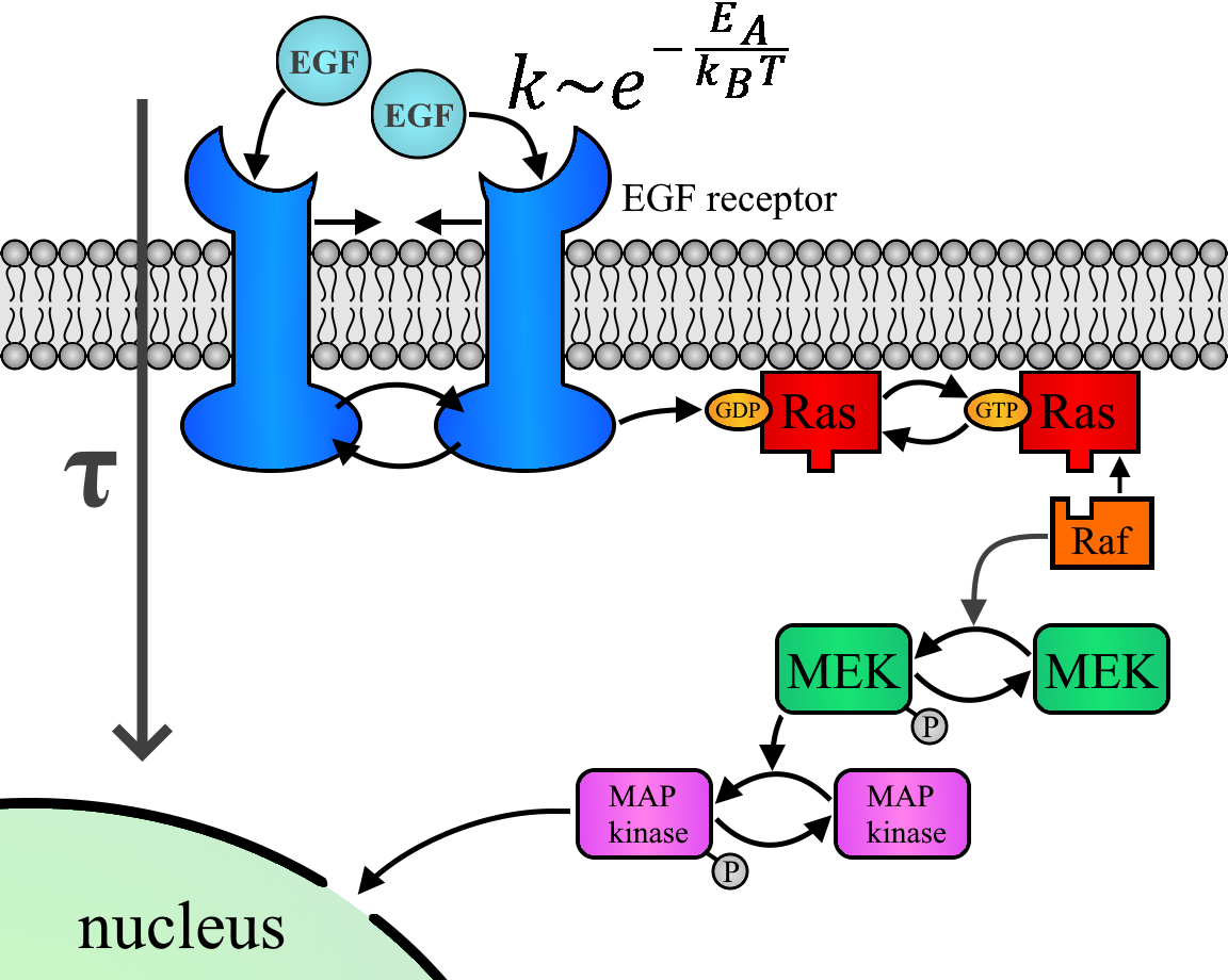
Indeed, certain features of the system Eq. (1) can be computed without the need for a complete solution [63]. A notable example are first-passage times (also called first-hitting times or exit times) [64, 65] and in particular, the mean first passage time (MFPT), which characterizes the typical completion time of the process of interest. The main example in this work is a developmental process seen as the consequence of a complex network of biochemical reactions. Developmental systems are very large and complex and besides biochemistry also involve many spatial processes, such as cytoskeletal rearrangements [66]. However, experimental measurement of heat generation in zebrafish embryos combined with modelling of biochemical networks suggests that even in this case, the rate-limiting steps are in the biochemical control system for the cell cycle [67], which in itself is again a large and complex biochemical network [68]. To give an instructive example of a small and transparent biochemical network that is active during development and that can be described with the master equation from Eq. (1), in Fig. 1 we show the mitogen-activated protein kinase (MAPK) signaling pathway triggered by epidermal growth factor (EGF). In this case, the MFPT describes the typical time for the signal to reach from the plasma membrane to the nucleus, where gene expression is changed. Here we ask who such MFPTs can be calculated for this and more complex networks, and how they depend on temperature.
II.2 Solution with graph theory
II.2.1 Some concepts from graph theory
It is often a useful approach to represent networks described by a master equation as weighted and directed graphs, i.e., vertices and directed edges (pairs of vertices), where the edges have a weight attributed to them [69]. Then the vertices are the states, the directed edges are the possible jumps and their weights are the jumping rates from vertex to vertex . In the following, graphs are always understood as weighted and directed. Also the rates are simply referred to as edges, for the ease of notation, setting if there is no transition from to .
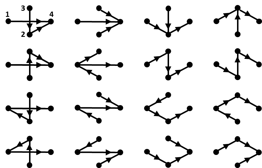
A tree rooted at a vertex is a cycle-free graph where there is a directed path from any other vertex to . Note that this requires to be an endpoint because any outgoing edge from would create a cycle. It is then also clear that the root of a tree is unique. A disjoint union of trees is called a forest. A spanning tree (forest) is a subgraph of a given graph that contains all its vertices and is a tree (forest). This is illustrated in Fig. 2.
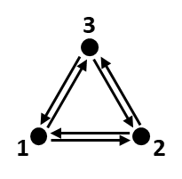
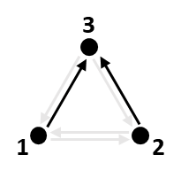
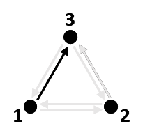
The (in-degree) Laplacian matrix of a graph is defined as:
| (4) |
so the -th entry on the main diagonal is the sum of all incoming edges and for are the negative transition rates from to .
II.2.2 Graph theoretical interpretation of FPT moments
The standard text book approach to find first-passage times (FPTs) is to evaluate them in Laplace-space[70, 65, 64]. However, this becomes increasingly cumbersome for larger systems. Here we instead use a solution that can be derived with graph theory [71, 72]. Consider the master equation on a finite space with time-independent rates . Then the formal solution to Eq. (2) is given by:
| (5) |
with exp denoting the matrix exponential and . Since , Eq. (5) can be restricted to only the first components. In particular, is then no longer singular.
Asking for the FPT to reach state , this state can be assumed to be absorbing, i.e., for all , because we are only interested in the first time that it is reached. The FPT density then follows from:
| (6) | ||||
| (7) |
where denotes the i-th unit vector. We define the FPT density to reach starting at state
| (8) |
where the second equality uses the symmetry of the inner product. In vector form, this now reads:
| (9) |
where . A distribution of this shape is called phase-type distribution[73]. The moments are obtained by integration by parts:
| (10) |
Equivalently we have
| (11) |
Here is the th moment of the FPT when starting at state . Iterative application of the formula above yields:
| (12) |
where . Note that
| (13) |
can be interpreted as the submatrix obtained by deleting the -th row and column of the Laplace matrix of the weighted and directed graph identifying the states with vertices and the edges with the transitions between them, where is the weight for the edge going from to .
By a generalization of Kirchhoff’s theorem to weighted and directed graphs[74], the determinant of is given by:
| (14) |
where denotes the spanning trees of the corresponding graph rooted at and their weights are defined as , with being the edge set of . Fig. (3) shows for the complete graph on four vertices as an example.
can be expessed as:
| (15) |
where is the determinant of the -minor of , which can also be expressed as a sum with a graph theoretic interpretation[71]:
| (16) |
where are the spanning forests with two trees of the graph, one rooted at and containing and the other one rooted at .
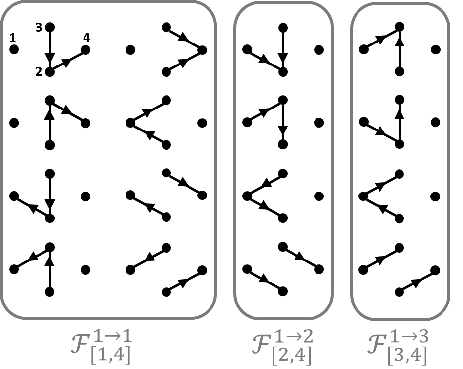
| (18) |
The mean in particular reads [71, 72]:
| (19) |
Note that similar graph theoretical counting schemes also exist for the steady state distributions of ergodic networks[75, 76]. In appendix A we show how this formula can be used to derive MFPTs for two example networks for which the results are also known from Laplace transforms.
Overall, the graph theoretical approach results in three possible approaches to the FPTs of a homogeneous master equation. The first one consists in solving the matrix exponential as given in Eq. (9) or, alternatively, the corresponding differential equation:
| (20) |
with as above. This is numerically feasible for systems of moderate size. If no full analytic solution is available, the moments of the FPT can be computed by either inverting algebraically and using Eq. (12) or by solving the combinatorial problem in Eq. (18).
First-passage time distributions can be broad, especially when one considers the statistics of rare events, and higher moments are therefore often of interest[64]. For processes with a clear bias towards a final state, the distribution of the completion time tends to be more narrow and its mean characterizes it sufficiently well[77], which is likely to be the case for most developmental systems. Indeed, the development times of Drosophila embryos varies only by a few percent[78].
II.3 Effect of temperature
Temperature now enters the description via the rate constants. By the Arrhenius equation[4], the temperature dependence of the can be described as follows:
| (21) |
where denotes the temperature, Boltzmann’s constant, a (temperature-independent) prefactor and is the activation energy. For large systems like developmental ones, one often expresses in . Then has to be replaced by the universal gas constant .
Since most biological organisms have evolutionary adapted to a relatively fixed thermal environment, it is reasonable to rephrase the Arrhenius equation in terms of the rate constant at a reference temperature , introducing . describes the temperature at which the organism usually operates. For instance, for homeothermic animals, the body temperature would serve as the natural reference point, while for poikilothermic animals, it would be the typical temperature of the environment. can be seen as the standard rates, and a crucial assumption for the following analysis is that these standard rates are independent of the activation energies .
The Arrhenius equation can be expressed in terms of these parameters as:
| (22) |
where .
II.4 Partition sums and generating functions
We note that the number of spanning trees on a complete graph on vertices is given by the Cayley formula[79] as , so it grows faster then exponential with . Even though many of the rates vanish, for sufficiently complex networks one can expect the numerator and the denominator of Eq. (19) to be the sum of many such graphs. This motivates the introduction of a partition sum like quantity summing over the spanning trees:
| (23) |
and for the two-tree spanning forests:
| (24) |
so that Eq. (19) reads in terms of these two quantities:
| (25) |
Letting the sums in Eq. (23) and Eq. (24) run only over the non-vanishing trees, all involved rates satisfy , and one can parameterize them as such that is the rate of interest. Applying this parametrization, one obtains for :
| (26) |
defining , which is the sum over all of a given tree. Now consider the Taylor-series of in :
| (27) |
The zeroth order coefficient is
| (28) |
i.e., it is the logarithm of the total number of spanning trees. For the first order, one finds:
| (29) |
i.e., the mean of over the trees. For the second order, one obtains:
| (30) |
i.e., the variance of over the trees. These results are no coincidence: Eq. (26) is precisely the cumulant generating function for such that one finds in general:
| (31) |
Hence,
| (32) |
and completely analogously for :
| (33) |
For the rates of interest (), the logarithm of Eq. (25) becomes:
| (34) |
Note that Eq. (34) is completely general and as such could be applied e.g. to the MAPK-system shown in Fig. 1. The cumulants are taken over the spanning trees and the expression is precise if all are known for any . Also, our treatment so far is not restricted to biochemical networks. In principle, it can also be applied to other settings described by a master equation.
II.5 Limit of large system size
We now are in a position to study the limit of large networks (). Because in this case not all details can be known, at the same time we switch to a statistical description for the reaction rates . To address temperature dependance, we consider biochemical networks with rates that have an Arrhenius-like temperature dependence, that is to say, , where and are assumed to be independent random variables. For that case, using that
| (35) |
where , one obtains:
| (36) |
Note that backward rates do not fully enter in the spanning trees (cf. examples in appendix A) so the activation energies on the trees and on the two-tree forests are different in general. The result so far requires to know the cumulants and to get the global rate constant. A priori, there may be infinitely many of them. But there are two cases in which the description simplifies:
Case 1: All are independent and identically distributed with no difference between the energies on the trees and the reduced trees. Then (seen as random variables) and Eq. (36) becomes:
| (37) |
again using the definition of the cumulant generating function.
For a developmental process, it seems rather reasonable to assume that the clear direction in the network is also reflected by the involved activation energies, so that the distributions of the forward and backward rates is different. Thus case 1 is therefore most likely not applicable to developmental systems.
Case 2: and can be sufficiently well approximated by normal distributions, and . Then all but the first two cumulants vanish, resulting in the following expression:
| (38) |
yielding a quadratic dependence in the Arrhenius plot (since ).
and are the sums of , and independent random variables and, since , the central limit theorem suggests indeed that this is a valid assumption. However, the crucial point here is that the higher cumulants have to vanish fast enough compared to the differences of the first two terms, requiring sufficiently well-behaved convergence to the normal distribution. The simplest case is that the already follow a normal distribution, which may be different for the on the trees and the two tree-forests, their sums also follow a normal distribution and one obtains:
| (39) |
We thus have arrived at our main result: the Arrhenius plot for large and complex biochemical networks is expected to show a quadratic dependence on the inverse temperature, if they have a bias towards a specific target state, as it must be the case for developmental systems.
II.6 Comparison to experimental data
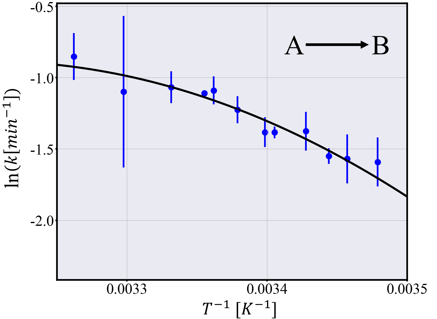
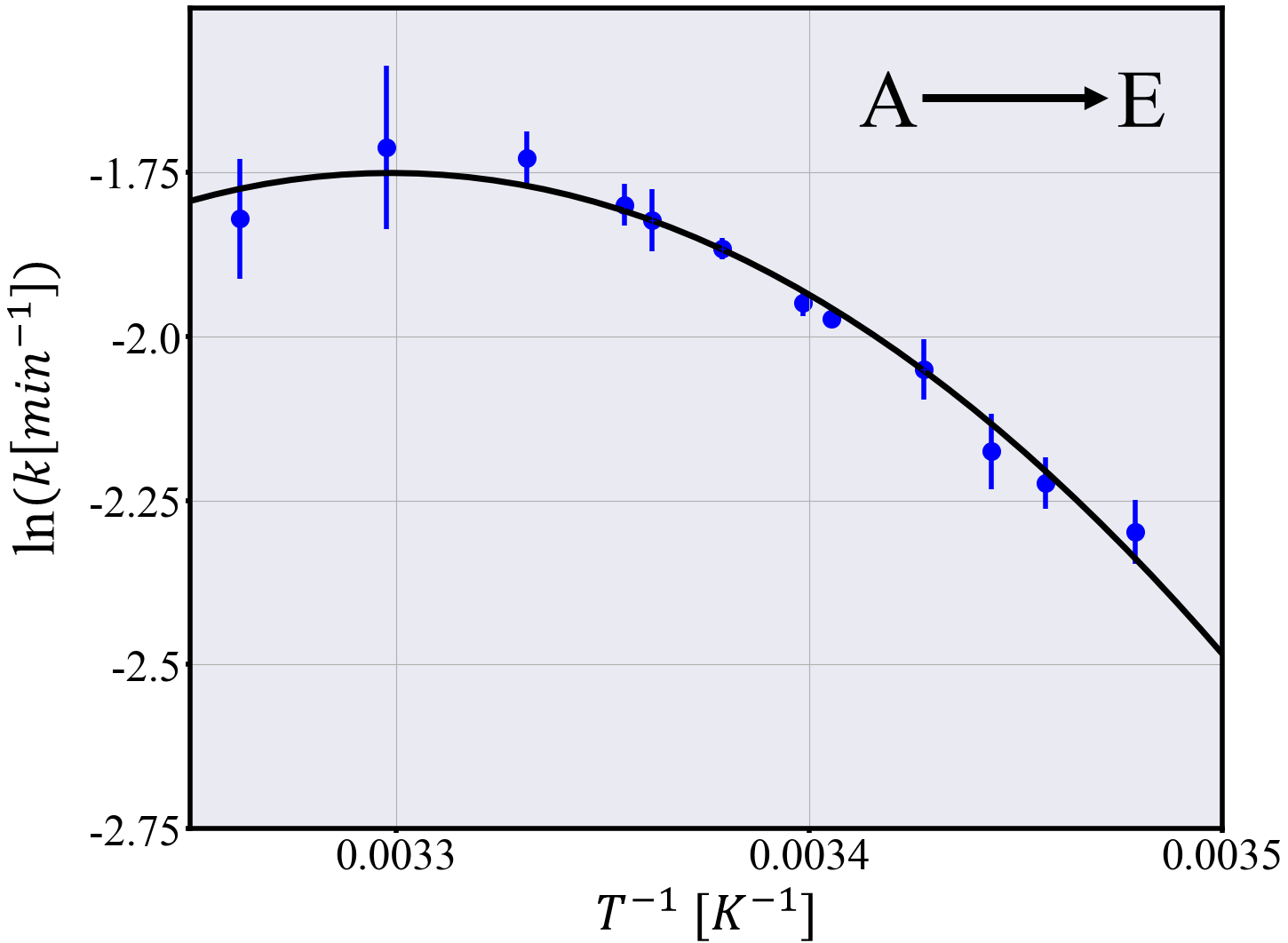
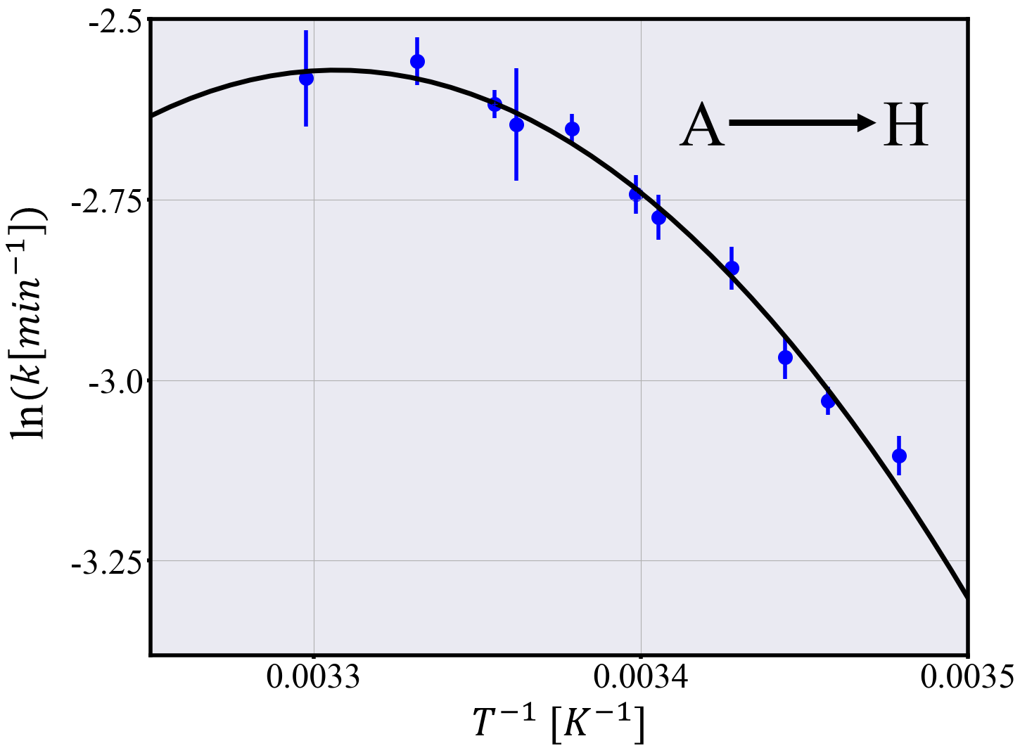
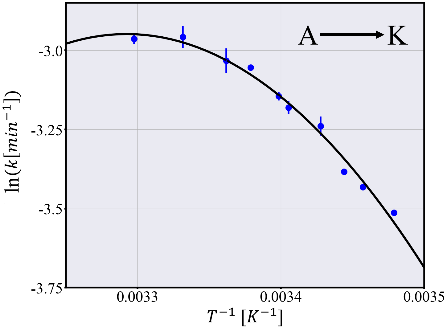
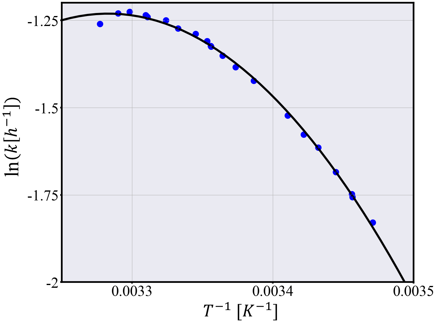
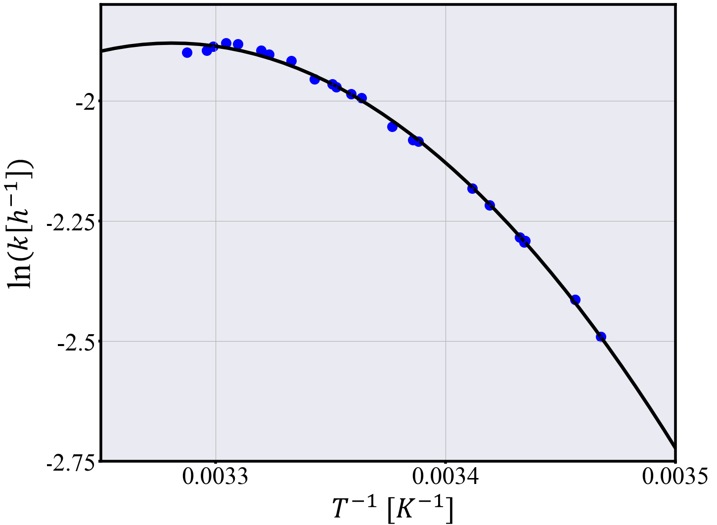
Indeed our theoretical prediction is in striking agreement with experimental data for developmental systems. In a work published in 2021, Crapse et al.[26] conducted a study on the development rates of Drosophila embryos at different temperatures. To that end, the embryonic phase of Drosophila was subdivided into 12 stages and the rates to reach each stage were measured under different temperature conditions. The 14th nuclear division in the zygote was chosen as the starting point (stage A) and the first breath was chosen as the end point (stage K). The cumulative rates starting with the 14th nuclear division to 4 different stages (B,E,H,K in the notation of the original authors) are shown in Fig. 5 as an example, together with a quadratic fit performed in Python via the numpy.poly1d command. The data were taken from the supplementary material of the original publication, which tabulated the measured times for the entire sample and all stages. The fitting parameters are listed in appendix C. Note that these do not provide insights into the microscopic structure of the network without further assumptions since the coefficients of the quadratic functions contain the differences of the first two moments along the trees and forests as well as terms containing .
For the beginning of stage B (begin of cellularization), no robust statement can be made about the goodness of the quadratic fit. Since this is the first stage following the starting point, it may well be that the assumption of a sufficiently large underlying biochemical network is simply not valid. However, as more steps accumulate, such as in the rates to stages E, H, and K, the quadratic shape of the data points becomes more apparent. A quadratic fit of the data was also suggested by Crapse et al.[26], although without providing an explanation on fundamental grounds, as done here.
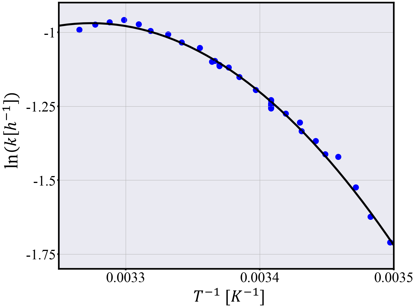
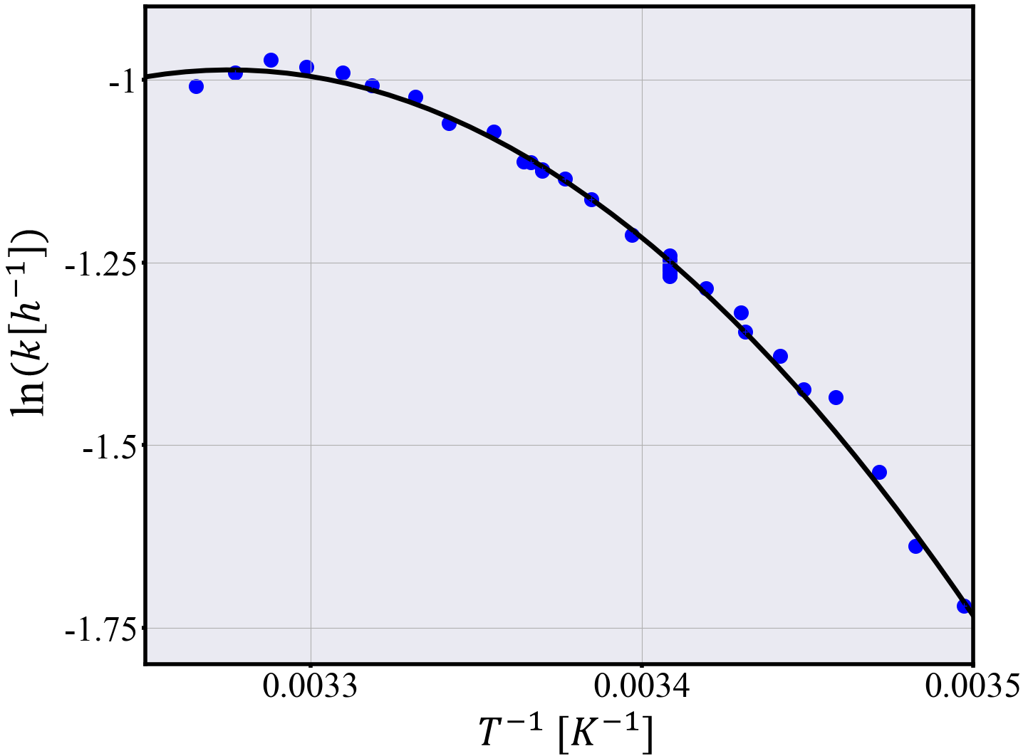
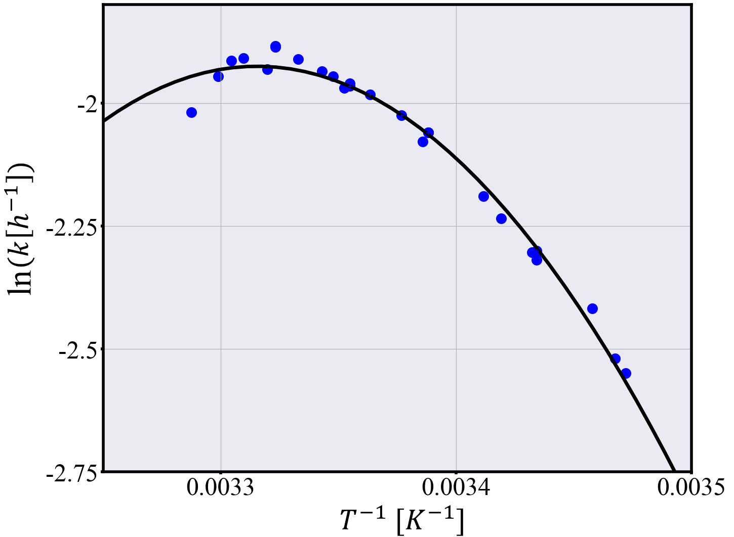
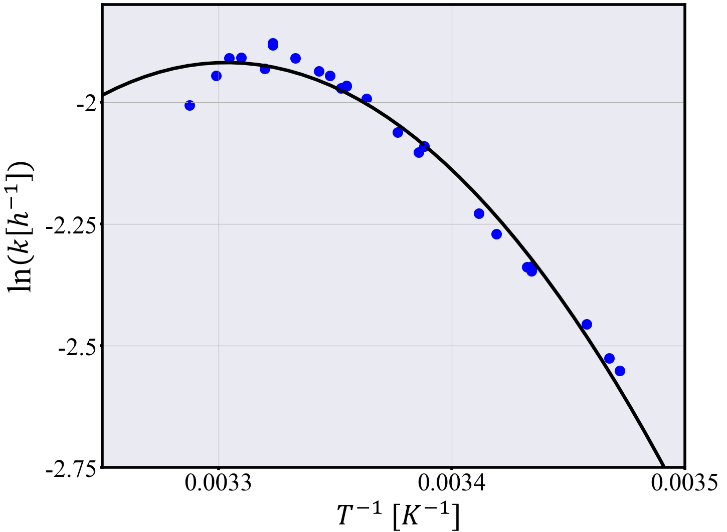
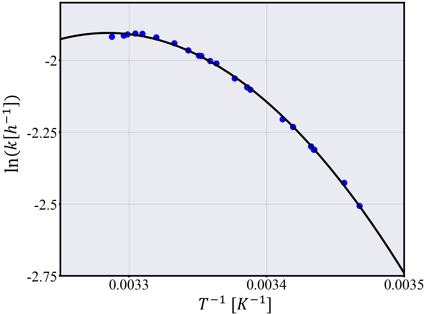
Measurements of the temperature dependence of developmental rates of Drosophila were already performed by Bliss[24] in 1926 for the prepupal development and by Powsner[25] in 1935 for the embryonic, pupal, and larval stages. Their results are shown in Fig. 6 and 7, respectively, also with a quadratic fit to their data points. Both articles list their data in a table and show them in a diagram, albeit together with piecewise linear functions as fit instead of a global quadratic function. One sees that in all cases, the quadratic fits predicted by our theory are in very good agreement with the experimental data.
III Discussion
Here we have shown that the generic temperature response of large biochemical networks is quadratic in the Arrhenius plot, if the network has an imbalance of activation energies in forward versus background directions, as it is to be expected for developmental systems. In order to make general statements on such networks, we resorted to a statistical description which does not require knowledge of all activation energies; rather we only make assumptions about their distribution, which is a reasonable description for a large system size , where not all degrees of freedom can be known. Our discussion was based on a general expression of the MFPT for arbitrary networks, Eq. (19), which follows from graph theory [72] and here has been derived in a pedagogical manner. We then rewrote this formula in the language of statistical physics. The coefficients appearing in the Taylor-series of the logarithmic MFPT can be interpreted in terms of the cumulants of the distribution of the sums along the spanning trees and two-tree forests. If this sum can be sufficiently well approximated by a Gaussian distribution, this yields a quadratic dependence in the Arrhenius plot, as described by Eq. (38). This is our main result, namely the quadratic response as the natural description for complex biochemical networks. This result would not apply for a network which has similar distributions for the activation energies for forward and backward directions, but this is unlikely for developmental systems.
Crapse et al.[26] suggested that the observed deviation from a pure Arrhenius-equation was due to the biochemical reactions not following an ideal Arrhenius-behavior, rather than a result of the complexity of the system. They reached that conclusion based on the simulation of a linear chain of reactions described by an Arrhenius-equation, which failed to reproduce the observed quadratic response in the Arrhenius plot. They also conducted an experiment measuring the conversion of NAD+ to NADH via GAPDH catalysis and found that this reaction does not follow a pure Arrhenius-like dependence. However, closer inspection of their simulations shows that the activation energies were chosen uniformly in an energy range from and the prefactors independently at . Due to the absence of backward rates and branching in this model, this leads to Eq. (37), for which the uniform distribution results in a series with infinitely many non-vanishing terms. If the activation energies were chosen from a normal distribution, this would yield a quadratic dependence also on this level. In contrast, our results are much more general and require less assumptions.
An important aspect of biochemical systems is that above the melting temperature of the involved proteins, the denaturation of the involved enzymes slows down the reaction rates quite substantially, which is not described by the Arrhenius equation [80, 81]. This could explain the curvature of the Arrhenius plots seen at small values of the inverse temperature, in particular for temperatures of about and above, where we observe that the high temperature data points (low inverse temperature) in Fig. 5-7 all lie below the quadratic curve. In the measurement by Powsner on the pupal development rates (Fig. 7B), the decrease is most notable, and it is not unlikely that this indicates that the denaturation threshold for a protein that is important for the developmental progression is surpassed at these temperatures. On the other hand, however, this observation also suggests that the larger part of the curve should not be affected by protein denaturation, and that our theory indeed captures the generic behaviour of this system. It should be mentioned that Powsner already noticed in his work that the combination of a few reactions, each described by an Arrhenius equation, does not necessarily yield a global Arrhenius equation and hypothesized that the observed temperature response may be a consequence of the complexity of the underlying biochemical network. However, he did not give an mathematical description as provided here. In the future, it might be interesting to extend our theory by the effect of protein denaturation, e.g. by introducing it as additional state in the network.
The observation that the development rates can be well described by a quadratic fit in the Arrhenius plot does not seem to be limited to Drosophila. Crapse et al.[26] provide similar results for the development of Xenopus laevis embryos, and Ratkowsky et al.[27] found empirically that the growth of bacterial colonies can be well described by a quadratic fit in an Arrhenius plot.
The discussion in this work was limited to the mean of the first-passage time, although our formalism in principle covers all higher moments, too. The focus on the first moment seems justified by the observation that the coefficient of variation (standard deviation divided by mean) for the development times of Drosophila embryos is in the order of a few percent across different temperatures[78]. This results most likely from a strong forward bias for the rates of a developmental network with many steps like cell cycle checkpoints and cell division being practically irreversible. It is well known and follows from our formalisms that this tends to yield sharp FPT distributions around the mean in the limit of large networks[77] (compare also the example in appendix B).
The framework developed in this work was motivated by describing the temperature dependence of complex networks where not all degrees of freedom are known. Here we focused on development, but as mentioned in the introduction, there exist other complex biological systems with interesting temperature dependence, in particular in the contexts of fever and climate change. We also note that our results are relatively general statements about the mean first passage time of master equations and are therefore not per se limited to biochemical networks and temperature effects. The idea to describe large reaction networks from a coarse-grained perspective with appropriate approximations has been discussed elsewhere [82], but neither the mean first passage time nor the possibility to describe the rate constants on a statistical basis the way proposed here seem to be explored so far. First passage-time problems are ubiquitous in biology and biochemistry [83] and it is very interesting how far one can get without knowing all the details of the system under consideration.
Acknowledgements.
JBV thanks the German Academic Scholarship Foundation (Studienstiftung des Deutschen Volkes) for support. We also acknowledge support by the Max Planck School Matter to Life funded by the German Federal Ministry of Education and Research (BMBF) in collaboration with the Max Planck Society.Appendix A Obtaining the MFPT by counting
To illustrate the application of the graph theoretical approach used here, we derive the MFPTs for two examples which also can be obtained by applying Laplace-transforms[77].
One-step master equation
Consider the one-step master equation with forward rates and backward rates as depicted in Fig. (8).

Note that there is only one spanning tree with all flow directed towards , namely the one consisting only of the forward rates, meaning that:
| (40) |
The are the chains which start off towards the right and switch their direction at and possibly also at a later vertex . This is shown in Fig. (9).

Simple Kinetic Proofreading
One can also derive the MFPT for a simple kinetic proofreading (KPR) scheme shown in Fig. 10 by correct counting.

Again, there is just one spanning tree, namely the one containing all . So one has again:
| (43) |
The are the graphs with forward rates up to some vertex and either or for any . This is illustrated in Fig. 11.

Therefore, one gets:
| (44) |
and obtains for the MFPT:
| (45) |
For the case that and , this expression simplifies to:
| (46) |
Appendix B First-Passage Times for a Linear Chain of Reactions
The simplest example of a large network is a linear chain of irreversible reactions, i.e., , as illustrated in Fig. (12)

Then the corresponding graph is already a tree and thus its own unique spanning tree:
| (47) |
Also, for the spanning forests it is easy to see that there is either exactly one or no combination:
| (48) |

Then,
| (49) |
One finds for the first two moments:
| (50) | ||||
| (51) |
which yields the standard deviation:
| (52) |
and the coefficient of variation (CV) reads:
| (53) |
meaning that for if most of the are of comparable sizes111One can find mathematical counterexamples otherwise, e.g., , which converges to , so the relative variation vanishes in the limit of large chains.
If , one finds in general:
| (54) |
which are precisely the moments for an -dimensional Erlang distribution (-distribution with non-negative integer as shape parameter) with :
| (55) |
as it should be since this is precisely the distribution that arises from summing up iid exponentially distributed random variables.
Note that the coefficient of variation (CV) reads:
| (56) |
so the relative deviation from the mean becomes increasingly small as the system size increases.
Appendix C Fitting parameters for quadratic fits in main text
The data in Fig 5-7 were fitted to a quadratic function of the shape . The corresponding parameters are listed in the two following tables:
| Figure | |||
|---|---|---|---|
| 5(a) | -1.06 | 0.68 | -1.10 |
| 5(b) | -1.81 | 1.19 | -1.98 |
| 5(c) | -1.96 | 1.30 | -2.17 |
| 5(d) | -1.71 | 1.13 | -1.88 |
| Figure | |||
|---|---|---|---|
| 6(a) | -1.48 | 0.97 | -1.60 |
| 6(b) | -1.47 | 0.97 | -1.59 |
| 6(a) | -1.48 | 0.97 | -1.60 |
| 7(a) | -1.74 | 11.39 | -1.88 |
| 7(b) | -2.62 | 1.73 | -2.89 |
| 7(c) | -2.36 | 1.56 | -2.59 |
| 7(d) | -1.80 | 1.18 | -1.96 |
| 7(e) | -1.75 | 1.15 | -1.91 |
References
- Blatteis [2003] C. M. Blatteis, Fever: pathological or physiological,injurious or beneficial?, in Journal of Thermal Biology 28 (2003).
- IPCC [2023] IPCC, Synthesis report of the ipcc sixth assessment report (ar6), in IPCC, Geneva, Switzerland. (2023).
- García et al. [2018] F. García et al., Changes in temperature alter the relationship between biodiversity and ecosystem functioning, Proceedings of the National Academy of Sciences 115, 10989 (2018).
- Arrhenius [1889] S. Arrhenius, Über die Reaktionsgeschwindigkeit bei der Inversion von Rohrzucker durch Säuren, in Z. Phys. Chem. 4: 226–248 (1889).
- Logan [1982] S. Logan, The origin and status of the arrhenius equation., Journal of Chemical Education 59, 279 (1982).
- Kramers [1940] H. Kramers, Brownian motion in a field of force and the diffusion model of chemical reactions, in Physica 7,4: 284-304 (1940).
- Hänggi et al. [1990] P. Hänggi, P. Talkner, and M. Borkovec, Reaction-rate theory: fifty years after kramers, Reviews of Modern Physics 62, 251 (1990).
- Eyring [1935] H. Eyring, The activated complex in chemical reactions, in J. Chem. Phys. 3 (2): 107–115 (1935).
- M. Polanyi [1935] M. E. M. Polanyi, Some applications of the transition state method to the calculation of reaction velocities, especially in solution, in Trans. Faraday Soc. 31: 875–894 (1935).
- Bichof and He [2006] J. C. Bichof and X. He, Thermal stability of proteins, Annals of the New York Academy of Sciences 1066, 12 (2006).
- Begasse et al. [2015] M. L. Begasse et al., Temperature dependence of cell division timing accounts for a shift in the thermal limits of c. elegans and c. briggsae, in Cell Reports 10, 647–653 (2015).
- Fujise et al. [0018] L. Fujise et al., Cell cycle dynamics of cultured coral endosymbiotic microalgae (symbiodinium) across different types (species) under alternate light and temperature conditions, in Journal of Eukaryotic Microbiology, 65: 505–517 (20018).
- Rieder and Maiato [2004] C. Rieder and H. Maiato, Stuck in division or passing through: Review what happens when cells cannot satisfy the spindle assembly checkpoint, in Developmental cell 7(5): 637-651. (2004).
- Moore et al. [1997] A. Moore et al., Effects of temperature shift on cell cycle, apoptosis and nucleotide pools in cho cell batch cultues, in Cytotechnology 23: 47–54 (1997).
- Hayashida et al. [1994] T. Hayashida et al., The ccgf/tae 250 gene is mutated in thermosensitive gl mutants of the bhk21 cell line derived from golden hamster, in Gene, 41: 247-270 (1994).
- Rao and Engelberg [1965] P. Rao and J. Engelberg, Hela cells: Effects of temperature on the life cycle, in Science 148(3673): 1092- 1094 (1965).
- Sisken et al. [1965] J. Sisken, L. Morasca, and S. Kibby, Effects of temperature on the kinetics of the mitotic cycle of mammalian cells in culture, in Experimental Cell Research 39, 103-116 (1965).
- Watanabe and Okada [1967] I. Watanabe and S. Okada, Effects of temperature on growth rate of cultured mammalian cells (l5178y), in J Cell Biol 32(2):309-23. (1967).
- Falahati et al. [2021] H. Falahati et al., Temperature-induced uncoupling of cell cycle regulators, in Dev Biol. 470: 147–153 (2021).
- Evans and Savage [1959] H. J. Evans and J. R. K. Savage, The effect of temperature on mitosis and on the action of colchicine in root meristem cells of vicia faba, in Experimental Cell Research 18, 51-61 (1959).
- et al. [2011] O. O. et al., Thermal robustness of signaling in bacterial chemotaxis, in Cell. 145(2): 312–321 (2011).
- Vanoni et al. [1984] M. Vanoni, M. Vai, and G. Frascotti, Effects of temperature on the yeast cell cycle analyzed by flow cytometry, in Cytometry 5:530-533 (1984).
- Zachleder et al. [2019] V. Zachleder et al., Cell cycle arrest by supraoptimal temperature in the alga Chlamydomonas reinhardtii, in Cells 8.10: 1237 (2019).
- Bliss [1926] C. Bliss, Temperature characteristics for prepupal development in drosophila melanogaster, in J Gen Physiol (1926) 9 (4): 467–495. (1926).
- Powsner [1935] L. Powsner, The effects of temperature on the durations of the developmental stages of drosophila melanogaster, in Physiological Zoology, Vol. 8, No. 4 (1935).
- Crapse et al. [2021] J. Crapse et al., Evaluating the arrhenius equation for developmental processes, in Mol Syst Biol. 2021 Aug;17(8):e9895 (2021).
- Ratkowsky et al. [1982] D. Ratkowsky et al., Relationship between temperature and growth rate of bacterial cultures, in ASM Journal of Bacteriology Vol. 149, No. 1 (1982).
- Johnson et al. [1974] F. Johnson, H. Eyring, and B. Stover, The theory of rate processes in biology and medicine (John Wiley and Sons, New York, 1974).
- Membré et al. [2005] J. M. Membré et al., Temperature effect on bacterial growth rate: quantitative microbiology approach including cardinal values and variability estimates to perform growth simulations on/in food, in International Journal of Food Microbiology 100: 179-186 (2005).
- Thormar [1962] H. Thormar, Effect of temperature on the reproduction rate of tetrahymena pyriformis’, in Experimental Cell Research 28, 269-279 (1962).
- Alberghina [1973] F. A. M. Alberghina, Growth regulation in neurospora crassa effects of nutrients and of temperature, in Arch. Microbiol. 89, 83–94 (1973).
- Yoshida et al. [2012] T. Yoshida et al., Temperature effects on the egg development time and hatching success of three acartia species (copepoda: Calanoida) from the strait of malacca, in Zoological Studies 51(5): 644-654 (2012).
- Choi et al. [2020] J. Choi et al., Probing and manipulating embryogenesis via nanoscale thermometry and temperature control, in Proc. Nat. Acad. Sci. USA: 117(26) (2020).
- Dell et al. [2011] A. Dell, S. Pawara, and V. Savage, Systematic variation in the temperature dependence of physiological and ecological traits, in Proc Natl Acad Sci USA 108 (26): 10591-10596 (2011).
- Hastings and Sweeney [1957] J. Hastings and B. Sweeney, On the mechanism of temperature independence in a biological clock, in Proc. Nat. Acad. Sci. USA: 43 (1957).
- Ruoff et al. [1997] P. Ruoff et al., Modeling temperature compensation in chemical and biological oscillators, in Chronobiol.Int.14, 499-510 (1997).
- Ruoff et al. [2000] P. Ruoff, M. Vinsjevik, and L. Rensing, Temperature compensation in biological oscillators: a challenge for joint experimental and theoretical analysis, in Comments Theor. Biol.5 , 361-382 (2000).
- Ruoff et al. [2003] P. Ruoff et al., Temperature dependency and temperature compensation in a model of yeast glycolytic oscillations, in Biophys Chem. 106 179–192 (2003).
- Virshup and Forger [2009] D. Virshup and D. Forger, Keeping the beat in the rising heat, in Cell. 137(4):602-4 (2009).
- Leloup and Goldbeter [1997] J. Leloup and A. Goldbeter, Temperature compensation of circadian rhythms: control of the period in a model for circadian oscillations of the per protein in drosophila, in Chronobiol.Int.14 511-520 (1997).
- Hong and Tyson [1997] C. Hong and J. Tyson, A proposal for temperature compensation of the circadian rhythm in drosophila based on dimerization of the per protein, in Chronobiol.Int.14 521-529 (1997).
- Pittendrigh [1954] C. Pittendrigh, On temperature independence in the clock system controlling emergence time in drosophila, in Proc. Nat. Acad. Sci. USA: 40 (10) (1954).
- Kidda et al. [2015] P. Kidda, M. Younga, and E. Siggiab, Temperature compensation and temperature sensation in the circadian clock, in Proc. Nat. Acad. Sci. USA: 112 (46) (2015).
- Vibe [2021] C. Vibe, The temperature response of the medaka segmentation clock and its link to robustness in embryonic patterning, Ph.D. thesis, University of Heidelberg, Germany (2021).
- Valeur and degli Agosti [2002] K. Valeur and R. degli Agosti, Simulations of temperature sensitivity of the peroxidase–oxidase oscillator, in Biophys.Chem.99 259-270 (2002).
- Ruoff [1992] P. Ruoff, Introducing temperature-compensation in any reaction kinetic oscillator model, in J.Interdiscipl.Cycle Res.23, 92-99 (1992).
- Oleksiuk et al. [2011] O. Oleksiuk et al., Thermal robustness of signaling in bacterial chemotaxis, Cell 145, 312 (2011).
- Bourn and Dorrity [2024] J. Bourn and M. Dorrity, Degrees of freedom: temperature’s influence on developmental rate, Current Opinion in Genetics & Development 85, 102155 (2024).
- Tyson et al. [2003] J. J. Tyson, K. C. Chen, and B. Novak, Sniffers, buzzers, toggles and blinkers: dynamics of regulatory and signaling pathways in the cell, Current opinion in cell biology 15, 221 (2003).
- Ratkowsky et al. [2005] D. Ratkowsky, J. Olley, and T. Ross, Unifying temperature effects on the growth rate of bacteria and the stability of globular protein, in Journal of Theoretical Biology 233: 351–362 (2005).
- Schoolfield et al. [1981] R. Schoolfield, P. Sharpe, and C. Magnuson, Non-linear regression of biological temperature-dependent rate models based on absolute reaction-rate theory., in Journal of Theoretical Biology, 88(4), 719-731 (1981).
- Wagner et al. [1984] T. Wagner et al., Modeling insect development rates: a literature review and application of a biophysical model., in Annals of the Entomological Society of America, 77,2: 208–220 (1984).
- Knies and Kingsolver [2010] J. Knies and J. Kingsolver, Erroneous arrhenius: Modified arrhenius model best explains the temperature dependence of ectotherm fitness, in Am Nat. 176(2): 227–233 (2010).
- Iyer-Biswas et al. [2014] S. Iyer-Biswas et al., Scaling laws governing stochastic growth and division of single bacterial cells, in Proc. Nat. Acad. Sci USA: 111(45) (2014).
- Quinn [2017] B. Quinn, A critical review of the use and performance of different function types for modeling temperature-dependent development of arthropod larvae, in Journal of Thermal Biology, 63, 65-77 (2017).
- Rebaudo and Rabhi [2018] F. Rebaudo and V. Rabhi, Modeling temperature-dependent development rate andphenology in insects: review of major developments,challenges, and future directions, in Entomologia Experimentalis et Applicata, 166(8), 607-617 (2018).
- Régnier et al. [2022] B. Régnier, J. Legrand, and F. Rebaudo, Modeling temperature-dependent development rate in insects and implications of experimental design, in Environ Entomol. 16;51(1):132-144 (2022).
- Yin et al. [1995] X. Yin et al., A nonlinear model for crop development as a function of temperature, in Agricultural and Forest Meteorology 77.1-2: 1-16 (1995).
- Zwietering et al. [1991] M. Zwietering et al., Modeling of bacterial growth as a function of temperature, in Applied and environmental Microbiology, 57,4: 1094-1101 (1991).
- Guerrero et al. [1994] F. Guerrero, J. M. Blanco, and V. Rodríguez, Temperature-dependent development in marine copepods: a comparative analysis of models, in Journal of Plankton Research 16,1: 95-103 (1994).
- Gillespie [1992] T. Gillespie, A rigorous derivation of the chemical master equation, in Physica A: Statistical Mechanics and its Applications 188: 404-425 (1992).
- Müller-Esterl [2018] W. Müller-Esterl, Biochemie (Springer Spektrum, 2018).
- Nam et al. [2022] K.-M. Nam, R. Martinez-Corral, and J. Gunawardena, The linear framework: using graph theory to reveal the algebra and thermodynamics of biomolecular systems, Interface Focus 12, 20220013 (2022).
- Redner [2001] S. Redner, A guide to first-passage processes (Cambridge university press, 2001).
- van Kampen [2004] N. van Kampen, Stochastic processes in physics and chemistry (North-Holland, 2004).
- Kanesaki et al. [2011] T. Kanesaki, C. M. Edwards, U. S. Schwarz, and J. Grosshans, Dynamic ordering of nuclei in syncytial embryos: a quantitative analysis of the role of cytoskeletal networks, Integrative biology 3, 1112 (2011).
- Rodenfels et al. [2019] J. Rodenfels, K. M. Neugebauer, and J. Howard, Heat oscillations driven by the embryonic cell cycle reveal the energetic costs of signaling, Developmental cell 48, 646 (2019).
- Ferrell et al. [2011] J. E. Ferrell, T. Y.-C. Tsai, and Q. Yang, Modeling the cell cycle: why do certain circuits oscillate?, Cell 144, 874 (2011).
- Lyons and Peres [2017] R. Lyons and Y. Peres, Probability on trees and networks, Vol. 42 (Cambridge University Press, 2017).
- Honerkamp [1996] J. Honerkamp, Stochastic dynamical systems: concepts, numerical methods, data analysis (John Wiley & Sons, 1996).
- Nam [2021] K. Nam, Algebraic approaches to molecular information processing, Ph.D. thesis, Harvard University (2021).
- Gunawardena and Nam [2023] J. Gunawardena and K. Nam, The linear framework ii: using graph theory to analyse the transient regime of markov processes, in Frontiers in Cell and Developmental Biology, 11, 1233808 (2023).
- Bladt and Nielsen [2017] M. Bladt and B. Nielsen, Matrix-exponential distributions in applied probability, Vol. 81 (Springer, 2017).
- Leenheer [2020] P. D. Leenheer, An elementary proof of a matrix tree theorem for directed graphs, SIAM Review 62, 716 (2020).
- Hill [1966] T. Hill, Studies in irreversible thermodynamics iv: diagrammatic representation of steady state fluxes for unimolecular systems., in Journal of Theoretical Biology, 10 (3): 442–459 (1966).
- Zia and Schmittmann [2007] R. Zia and B. Schmittmann, Probability currents as principal characteristics in the statistical mechanics of non-equilibrium steady states, in J. Stat. Mech. P07012 (2007).
- B. Munsky [2009] G. B. B. Munsky, I. Nemenman, The simplicity of completion time distributions for common complex biochemical processes, in Physical biology 7.1: 016003 (2009).
- Chong et al. [2018] J. Chong, C. Amourda, and T. Saunders, Temporal development of drosophila embryos is highly robust across a wide temperature range, Journal of the Royal Society Interface 15, 20180304 (2018).
- Cayley [1889] A. Cayley, A theorem on trees, in Quart. J. Math. 23:376-378 (1889).
- Lepock [2005] J. Lepock, Measurement of protein stability and protein denaturation in cells using differential scanning calorimetry, in Methods 35: 117– 125 (2005).
- Mateus et al. [2018] A. Mateus et al., Thermal proteome profiling in bacteria: probing protein state in vivo, Molecular systems biology 14, e8242 (2018).
- Kulasiri and Kosarwal [2021] D. Kulasiri and R. Kosarwal, Chemical Master Equation for Large Biological Networks: State-space Expansion Methods Using AI (Springer Singapore, 2021).
- Polizzi et al. [2017] N. Polizzi, M.J.Therien, and D. Beratan, Mean first-passage times in biology, in Isr J Chem. 56 (9-10):816-824 (2017).
- Note [1] One can find mathematical counterexamples otherwise, e.g., , which converges to .