Quasiprobabilities in quantum thermodynamics and many-body systems: A tutorial
Abstract
Quasiprobabilities are mathematical quantities describing the statistics of measurement outcomes evaluated at two or more times, which incorporate the incompatibility of the measurement observables and the state of the measured quantum system. In this tutorial, we present the definition, interpretation and properties of the main quasiprobabilities known in the literature. We also discuss techniques to experimentally access a quasiprobability distribution, ranging from the weak two-point measurement scheme, to a Ramsey-like interferometric scheme and procedures assisted by an external detector. Once defined the fundamental concepts following the standpoint of joint measurability in quantum mechanics, we illustrate the use of quasiprobabilities in quantum thermodynamics to describe the quantum statistics of work and heat, and to explain anomalies in the energy exchanges entailed by a given thermodynamic transformation. On the one hand, in work protocols, we show how absorbed energy can be converted to extractable work and vice versa due to Hamiltonian incompatibility at distinct times. On the other hand, in exchange processes between two quantum systems initially at different temperatures, we explain how quantum correlations in their initial state may induce cold-to-hot energy exchanges, which are unnatural between any pair of equilibrium non-driven systems. We conclude the tutorial by giving simple examples where quasiprobabilities are applied to many-body systems: scrambling of quantum information, sensitivity to local perturbations, quantum work statistics in the quenched dynamics of models that can be mapped onto systems of free fermions, for instance the Ising model with a transverse field. Throughout the tutorial, we meticulously present derivations of essential concepts alongside straightforward examples, aiming to enhance comprehension and facilitate learning.
I Introduction
In this paper we provide a tutorial that delves into the use of quasiprobabilities and their associated distributions within the realm of quantum science and with specific applications in quantum thermodynamics and many-body quantum systems.
As evident from numerous studies [1, 2, 3, 4, 5, 6, 7, 8, 9, 10, 11, 12, 13, 14, 15, 16, 17, 18], quasiprobabilities have garnered significant interest within the quantum community. In fact, they are a proper tool to describe the statistics of the outcomes resulting from consecutive events in several areas of quantum mechanics and associated technologies, from foundations to quantum devices. The most appealing feature of a quasiprobability is its capability to embody the incompatibility of quantum observables, due to their nonzero commutator, that are evaluated at different times of a given experiment. This incompatibility is singled out by the fact that the distribution of the measurement outcomes admits non-classical traits. The latter ones, expressed in the form of ‘negative’ and ‘non-real probabilities’, reflect the effects entailed by the Heisenberg uncertainty principle that indeed concerns the impossibility of concurrently measuring two complementary and incompatible properties of a quantum system in contiguous times.
In the following, we are going to introduce the concept of quasiprobability from theoretical arguments, and we then outline their main properties, especially those concerning the loss of positivity. After that, we will address measurement procedures that allow to observe the ‘negative’ and ‘non-real probabilities’ of pairs of measurement outcomes, by showing that such genuinely quantum features have a clear physical interpretation inherently related to quantum coherence and correlations. We are particularly interested in pedagogically explaining those physical interpretations that can be linked to thermodynamic quantities under out-of-equilibrium conditions (work, heat and their distributions) [19, 5, 8, 20, 21, 22, 12, 15], and in the rich arena of many-body quantum systems [4, 23, 6, 11, 14, 16, 17]. In this regard, interpretations of the well-known Loschmidt echo and out-of-time-ordered correlators (OTOCs) for many-body systems in term of quasiprobabilities are discussed and illustrated with step-by-step worked examples. Finally, the tutorial is concluded with a discussion containing some perspectives on possible theoretical studies and experimental observations of quasiprobabilities in current quantum platforms [24, 22, 12].
This tutorial is targeted at graduate students and researchers, both theoretical and experimental, with a basic knowledge of quantum mechanics. Specifically, we aim to provide both the formal definitions that lay the foundations for quasiprobabilities in quantum science, and simple analytical examples helping understanding the fundamental concepts and applications of the methodology. We would also give some hints on new directions on the use of quasiprobabilities that have not yet been explored, especially in quantum thermodynamics and many-body quantum systems.
II Quasiprobabilities
In this section, we introduce the concept of quasiprobabilities in quantum mechanics, following the seminal papers by Kirkwood [25] and Dirac [26] in the 30’s and 40’s, respectively. There have been several approaches that brought to light the notion of a ‘negative probability’ and crucially even probabilities represented by a complex number. In this tutorial, we choose to approach this topic from the fundamental standpoint of joint measurability in quantum mechanics.
Under conditions we are going to detail, Kirkwood-Dirac quasiprobabilities (KDQ) can take both negative and imaginary values. ‘Negative probability’ and even ‘probabilities represented by a complex number’ can be explained from the fundamental standpoint of joint measurability in quantum mechanics.
For this purpose, let us set the theoretical framework. First, consider a quantum state preparation that generates a generic density operator that, by definition, is a Hermitian, semi-definite operator with trace . Then, we define two quantum observables, associated to two Hermitian operators, and , that we measure at two distinct times and with . The observables can be generally expressed using their spectral decomposition as
| (1) |
in terms of their eigenvalues and the associated projectors onto the corresponding eigenspace.
In the general case, , and do not commute with each other. Moreover, in the time interval —after the first measurement of and before the second measurement of —the state of the quantum system can be subject to a generic quantum process described by a completely positive trace preserving (CPTP) quantum map , which operates on and returns density operators. We introduce its Kraus representation such that and , where is the identity operator. The reader interested in the main properties of quantum maps can refer to Refs. [27, 28].
In this Section, we discuss how to characterize the statistics of measurements outcomes from the -time evaluation of and , by also taking into account the non-commutativity of the involved operators, i.e., the initial density operator and the two observables. We explicitly wrote “-time evaluation” in order to clearly distinguish it from the wording sequential measurements. In fact, as we will explain in a while, a procedure based on sequential measurements is necessarily invasive. As a result, (a) the measured system is perturbed; (b) initial quantum coherence in (with respect to the basis decomposing ) is destroyed; (c) the statistics of the outcome pairs resulting from sequentially measuring and changes.
Because of these reasons, we are going to consider an approach that, even in the general non-commutative case, can return a statistics of that is exempt from the invasiveness of the measurement apparatus, and is not affected by the first measurement of a sequential procedure, at least in some statistical moments [29]. This aspect should not be surprising since it is known that [30] when non-commuting observables are taken into account, there is no unique formula to describe the joint probabilities of that has both a correspondence with the classical theory of probability and at the same time is returned by a non-invasive measurement routine; see Sec. II.2 for more details on this aspect.
Now let us discuss in greater depth the invasiveness under the joint measurability problem, by introducing the celebrated two-point measurement (TPM) scheme [31].
II.1 Sequential projective measurements and the TPM scheme
The TPM scheme is the procedure to characterize the statistics of by means of sequential measurements, which has a correspondence with the classical theory of probability [32]. Albeit the process underlying the measurement outcomes has quantum traits, the results from such measurement procedure can be also described by a probability distribution that obeys the Kolmogorov’s axioms of probability. The Kolmogorov’s axioms are: (i) the probability of getting a measurement outcome is a non-negative real number; (ii) the probability to measure at least one of the outcomes is ; (iii) the probability to measure any countable sequence of mutually exclusive measurement outcomes is equal to the sum of the probabilities for each outcome.
Operationally, the two quantum observables and are measured at times and , respectively, and a pair of outcomes is obtained. The probability distribution associated to any outcome pair is determined by repeating the sequential measurement procedure several times. Formally, the joint probability to get , according to the TPM scheme, is
| (2) |
where is the initial quantum state (prepared at time ), and is one of the two projectors of evolved in Heisenberg the picture. For unitary dynamics, , where we have introduced the unitary evolution operator of the system with denoting the reduced Planck’s constant, set to 1 for simplicity from now on, the time-ordering operator and the Hamiltonian of the system at time .
A procedure based on sequential measurements is invasive as it violates the no-signaling in time condition [33]. If applied to our case-study, the no-signaling in time condition states that the statistics of that is returned by a non-invasive measurement apparatus must fulfill the condition
| (3) |
where stands for a generic joint probability. In other terms, the requirement for the non-invasiveness is that, marginalizing the distribution over the outcomes of the first observable at time , we recover the unperturbed single-time probability associated to the outcomes of the second observable at .
In this respect, non-invasiveness can be considered as a synonymous of unperturbed marginals. The validity of Eq. (3) is a necessary condition for macrorealism [34] and, interestingly, Eq. (3) can be violated even in situations where no violation of Leggett-Garg inequalities is allowed [33]. The violation of the no-signaling in time condition marks the main consequence of the joint measurability problem due to the incompatibility of the involved quantum operators , and .
The question that now arises is: “What information is erased by using the TPM scheme in the attempt of attaining the statistics of ?” or equivalently “How invasive is a procedure based on sequential measurements?” We are going to show that the TPM scheme is non-invasive if and only if or . Otherwise, Eq. (3) would be violated. In order to determine what information is erased by the TPM scheme, let us compare the final-time probability and . The latter equals
| (4) |
where the super-operator
| (5) |
denotes the dephasing channel, which is defined over the eigenbasis of the quantum observable and is applied to the initial density operator . In Eq. (5), . Hence, if we compare and , we can see that the first measurement of the TPM scheme erases the quantum coherence contained in once projected onto the eigenbasis of .
It is worth noting that the initial density operator can always be linearly decomposed in the basis of as
| (6) |
where
| (7) |
is the operator containing the off-diagonal elements of , with .
As an example, let us consider a qubit as the quantum system and as the quantum observable at time . We have introduced the Pauli matrices 111 Throughout the tutorial, we recall that any Pauli matrix along the -, - and -axis (i.e., , or ) is a complex operator that is Hermitian (), involutory () and unitary ( entailing that ).. Then,
| (8) |
where , are the two eigenstates of , , and, due to the Hermiticity of , .
II.2 No-go theorem for sequential outcomes statistics
Previously, we have outlined that a procedure based on sequential measurements fails in recovering the marginal distribution of the pairs with respect to the measurement outcomes of . This directly violates the no-signaling in time condition Eq. (3), and establishes that the measurement procedure is invasive. The origin of such violation lies in the fact that at least one of the commutators and is different from zero.
This conclusion is related to a deeper statement summarised by the no-go theorem reported in Ref. [11], which is less restrictive than the formulation firstly proven in Ref. [36]. The no-go theorem states that the following three properties cannot be valid simultaneously for any initial density operator if and only if for some pair :
-
i)
The probability distribution of the pairs , defined by the generic joint probabilities in the time interval , obeys the Kolmogorov’s axioms of the classical theory of probability.
-
ii)
The joint probabilities lead to unperturbed marginals:
(9) (10) -
iii)
The joint probabilities are linear functions of the initial density operator . Formally, this means that, given a linear combination , then .
The three properties i)-iii) are all simultaneously satisfied under the assumption of the commutative condition , and the probability distribution that fully characterizes the statistics of the pairs is the one returned by the TPM scheme.
In the following and throughout the tutorial, we will give up the property i). As a consequence we can no longer employ sequential measurements to characterize the statistics of . Avoiding the direct application of the TPM scheme on the quantum system under scrutiny may completely eliminate the invasiveness of the measurement procedure and allow us to recover unperturbed marginal distributions [property ii)]. Such a requirement for the generic joint probabilities is well-justified if we want that our knowledge on the fluctuations of the pairs is not decreased by the quantum measurement back-action. We therefore require that the no-signaling in time condition is fulfilled. Furthermore, we demand that the probability distribution of exhibits linearity, in conformity with the property iii). In this way, for any variation of , one does not need to repeat from scratch the experimental procedure (which, as noted earlier, should not be sequential) to determine .
As a result, by linearly decomposing as in Eq. (6), in terms of its diagonal and off-diagonal parts with respect to the eigenbasis of , we recover the results of the TPM scheme whenever , with denoting the matrix with all zeros. In addition, another consequence of the linearity property is that the procedure for measuring can be independent on the initial density operator , as it is customary in the classical case.
II.3 Beyond the two-point measurement scheme: Quasiprobability approach
Under the non-commutativity hypothesis for some pair , dropping the property i) of the no-go theorem mentioned in Sec. II.2 allows for the introduction of a quasiprobability distribution (QD), whose terms can be non-positive (i.e., negative real numbers or even complex numbers), albeit still summing to . In general, there is not a unique QD due to ordering ambiguities in how the QD is defined (see Refs. [30, 9, 10, 13, 11]). As a consequence, there are, in principle, infinite QD that are linear in the initial state and lead to unperturbed marginals, at both the initial and final times and .
Let us introduce the quasiprobabilities. We start from the expression for the generic joint probabilities and assign a linear operator to each pair of measurement outcomes. Without loss of generality, we can write:
| (11) |
From classical probability theory, in the case of the TPM scheme [see Sec. II.1], we find that
| (12) |
that returns Eq. (2). Instead, we obtain a quasiprobability by setting either
| (13) |
or
| (14) |
Substituting the linear operators or in Eq. (11) gives two perfectly valid KDQ. The difference of applying or on is that they operate on off-diagonal terms of with exchanged indexes []. In fact, one can prove that
whence
| (15) |
thus meaning that the KDQ and differ by their imaginary parts that are opposite in sign.
Both KDQ reduce to , as in Eq. (2), if or . In this tutorial, without loss of generality, we will make use of the KDQ defined by that, from now on, we denote as
| (16) | |||||
The sign ambiguity in and can be overcome by taking the uniformly-weighted sum of and , i.e.,
| (17) | |||||
where denotes the anti-commutator of the generic operators . In this way, we end-up with the quasiprobability
| (19) |
commonly known as the Margenau-Hill quasiprobability (MHQ) [37].
Other quasiprobabilities have been considered in the literature for systems weakly interacting with a detector in order to avoid the invasiveness of the first measurement of the TPM scheme [38, 39, 19, 40, 41, 42, 21]. We will discuss them in detail in Sec. III.
The quasiprobabilities defined in Eq. (16) and Eq. (19) respect properties ii) and iii) of the no-go theorem in Sec. II.2, meaning that the no-signaling in time condition is fulfilled and the measurement procedure that allows to get a QD is independent of the initial state . Moreover, the TPM statistics is recovered in the case in which , , all commute with each other.
These characteristics are important requisites to build a consistent thermodynamic theory via quasiprobabilities. In fact, any dependence of thermodynamic quantities—work, heat and entropy—on the initial state seems to be in contradiction with their standard definition in classical thermodynamics that does change depending on the particular phase-space distribution taken as the input ensemble.
II.3.1 Non-positivity
KDQ naturally encode temporal correlations between outcomes of the measurements of the quantum observables and . As explained in Sec. II.2, in relation to the no-go theorem, the quasiprobabilities can be non-positive, although they are still subject to the normalisation constraint
| (20) |
In the case of KDQ, non-positivity can mean the following two facts:
-
I)
the real part of is negative;
-
II)
is a complex number with a nonzero imaginary part.
From a mathematical point of view, the onset of non-positivity in KDQ is a consequence of the fact that the product of two quantum observables (say, and ) can always be decomposed as the linear combination of self-adjoint operators as . Thus, for the product , we have
| (21) |
The first term on the right-hand-side of Eq. (21) gives rise to the MHQ, the real part of the KDQ, when evaluated (i.e., averaged) with respect to the initial density operator . Moreover, looking at the second term of Eq. (21), it is evident that a necessary condition for the KDQ to have an imaginary part is the non-commutativity of and . In this regard, we stress that if , then , and the KDQ coincides with the TPM probabilities. Furthermore, in order to ensure the validity of Eq. (20), the imaginary parts of KDQ must cancel each other out.
In Sec. II.3.2, we will show a simple case-study that directly connects the imaginary part of the KDQ with the presence of imaginary coherence terms in the initial density operator , with respect to the eigenbasis of . Hence, if we ignored the imaginary parts of , we would exclude some information stemming from quantum coherence and correlations that may emerge in the quantum statistics of . The occurrence of non-positivity can be considered as a non-classical feature in the statistics of the measurement pairs, underlining the presence of genuinely quantum features due to the interplay of quantum dynamics and measurement. From here on, we will refer to this with the term non-classicality.
Non-commutativity is a necessary condition.
In this context, for the MHQ , see Eq. (19), it has been recently shown that the pairwise non-commutativity of the initial density operator and the quantum measurement observables is only a necessary but not sufficient condition for non-positivity (i.e., negativity of the MHQ). This means that there are counterexamples where and/or , but still . A detailed analysis of this aspect can be found in Ref. [9], where it has been formulated with the wording negativity is stronger than non-commutativity.
Linear positivity.
The fact that the non-commutativity is only necessary condition for negativity is strongly linked with the findings in Ref. [43] by Goldstein and Page. They recognised that non-commutativity conditions, a hallmark of the non-classicality defined above, can coexist with to some extent. In other words, there can be time intervals of a given dynamical evolution of the quantum system under scrutiny where the occurrence of is described by positive probabilities. In view of this argument, Goldstein and Page introduced the concept of linear positivity [43] to single-out the weakest conditions under which positive MHQ can be assigned to the statistics from non-commuting observables.
Direct link with weak values.
Finally, the non-positivity of KDQ can find a physical interpretation from their direct connection with weak values [44, 45, 46] that, indeed, are conditional KDQ [11]. To see this, we set , where , under the hypothesis that the dynamics is unitary, and is a rank-1 projector. Moreover, we take as a pure state. Hence, from Eq. (16) one has that
| (22) |
where
| (23) |
is the original definition of the weak value (WV) of the projector with initial state and post-selection . In this way, the weak value of the observable is obtained by averaging the outcomes over the conditional KDQ . Formally, we have that
| (24) |
We recall that the weak values are obtained via a weak measurement that is performed on both a properly chosen pre-selected quantum state and a post-selected one. Weak values are called anomalous when lies outside the spectrum of (see Refs. [47, 48, 49, 50]). In order to guarantee such anomaly, it is required that the (possibly mixed) pre- and postselection states have quantum coherence with respect to the eigenbasis of [51]. Moreover, the generalization of weak values to mixed density operators instead of pure quantum states, can be a complex number, and this is evidently in a one-to-one correspondence with complex KDQs [52, 53, 47, 49].
Non-positivity functional.
We conclude this subsection by discussing the non-positivity of KDQ. For this purpose, we introduce the non-positivity functional [54, 9, 12, 11]
| (25) |
that quantifies the ‘amount’ of non-classicality in the statistics of the outcome pairs . It is worth noting that both the real and imaginary parts of the KDQ contribute to the non-classicality, whereby if present one has that
| (26) |
Instead, when all the KDQ are positive real numbers 222The positivity meant here goes beyond the notion of ‘linear positivity’ by Goldstein and Page [43], since for KDQ also imaginary parts are taken into account, and not only the negativity of the real part of ..
II.3.2 Comparing KDQ and TPM probabilities
In this subsection we are going to compare the KDQ with the joint probabilities returned by applying the TPM scheme. In this regard, notice that
| (27) |
where
| (28) |
is the projector orthogonal to . Interestingly, as discussed in Ref. [30], Eq. (27) quantifies the interference patterns between the two different sequential pairs of projectors, also known in the literature as quantum histories, and . Moreover, the right-hand-side of Eq. (27) is also recovered from the so-called non-demolition quasiprobability (NDQP) [56, 19, 21]
| (29) |
with . The NDQP is evidently defined over three indexes: two, and (different each other), refer to two possible measurement outcomes of the quantum observable at time , while refers to as it holds for . Thus, by marginalizing over , one directly obtains the difference between the KDQ and TPM (joint) probabilities:
| (30) |
It can be easily observed that if , then necessarily ; moreover, when the KDQ is a complex number, also is a complex number with the same imaginary part of .
Let us now exemplify these concepts with a simple case-study. Let us consider a spin- particle, first initialized in the generic density operator . Then, the spin of the particle is consecutively measured along two orthogonal axes, the - and -axis, respectively, i.e. and . Moreover, we assume , so that the system does not evolve between and . Note that, under specific conditions [57], this set-up is representative of the physics underlying the well-known Stern-Gerlach experiments.
At the end of this quantum process, the state of the system collapses onto one of the eigenstates of , namely and , with . Let us denote the eigenvalues of the observables and with , and , , respectively. The quantum process is inherently probabilistic, due to the stochastic nature of any quantum measurement. We thus need to calculate the probabilities of obtaining the pairs of measurement outcomes measured at times and with and , for the initial density operator .
As previously anticipated, if , then the application of the TPM scheme (i.e., sequential measurements) does no longer suffice. This fact is confirmed by the direct computation of the differences :
| (31) | |||||
| (32) | |||||
| (33) | |||||
| (34) |
where, by construction, .
From Eqs. (31)-(34), it is also apparent that at least two of the differences , among all four, exhibit negative real parts whenever the initial state does not commute with the quantum observable at time . Notably, such a negativity is preserved from applying a second measurement of the observable immediately after the first.
Of course, in the case , the KDQ reduces to the TPM joint probabilities , and the no-signaling in time condition is fulfilled. On the contrary, in the case , the first measurement of of the TPM scheme turns out to be invasive for the joint statistics of the measurement outcomes .
Finally, we conclude this analysis by providing the average of the difference of outcomes (thus, ) that is evaluated with respect to the KDQ . We have
| (35) | |||||
By setting , it holds that that stems from having all the KDQ equal to . This finding is in accordance with the classical theory of probability applied to our case-study. In fact, if the initial density operator of the spin- is mixed with both elements equal to (i.e., the spin of the particle is initially up or down with equal probability ), then the sequence of measurement outcomes obtained from applying two mutually uncorrelated operations (i.e., the sequential projective measurement of and ) is naturally equiprobable. As a result, on average the difference of the measurement outcomes is zero.
Let us now add quantum coherence to the initial state with respect to the eigenbasis of , by taking
| (36) |
with defined in Eq. (8). Hence, from Eq. (35), we obtain , meaning that a correction to the “classical” result has to be included. In this case-study, such a correction is directly proportional to the quantum coherence of .
II.3.3 Distribution and characteristic function of KDQ
As mentioned in the previous sections, the KDQ describes the joint probability of the pairs of outcomes from measuring the quantum observables and at times and , initial and final times of the quantum process in analysis, with . The individual outcomes and correspond to the eigenvalues of the observables in Eq. (1).
Let us introduce the generic difference of outcomes
| (37) |
such that . The number of values that can take depends on the combinations of all possible measurement outcomes at . Therefore, the KDQ distribution of is defined by
| (38) |
where is the Dirac delta function. We remark that the KDQ distribution is not unique due to ordering ambiguities entailed by the non-commutativity of , and , as discussed in Sec. II.3. We also note that the distribution of provided by the TPM scheme is
| (39) |
where, as before, denotes the TPM joint probabilities.
All the information about the statistics of the outcome pair is also encoded in the characteristic function of defined as its Fourier transform:
| (40) | |||||
While in principle for a Fourier transform the variable is real, it may be useful to extend Eq. (40) with as a complex number, as we will see in Sec. IV.2. Interestingly, both the KDQ and the characteristic function are quantum correlation functions, namely they can be obtained as the expectation value of the product of two operators, not necessarily Hermitian, but defined at two times, on the initial density operator . In general, the distribution depends on the time duration of the quantum system dynamics. Of course, the time-dependence of is mirrored in a time-dependent characteristic function . Both for and , the time-dependence is omitted, unless specified to enhance the clarity of the presentation.
III Measuring quasiprobabilities
In this section, we are going to present two methods that allows the reconstruction of a QD: the first is based on performing only projective measurements [58, 12], while the second is aimed at measuring directly the characteristic function of the QD under scrutiny. More than these two approaches have been formulated so far to achieve such a reconstruction [59, 60, 61, 62, 63, 64]; the reader can find more details in Ref. [11] where these methods have been surveyed and some of them extended. Moreover, it is also worth mentioning Ref. [65] that investigates the use of quantum circuits for the measurement of weak values and KDQ distributions.
III.1 Weak two-point measurement scheme
It can be proved that the real part of the KDQ distribution, defined in Sec. II.3 as the Margenau-Hill (MH) distribution, can be determined by resorting only to a scheme entirely based on projective measurements. We have already proved that a direct sequential measurement procedure cannot carry out this task. Instead the combination of projective measurement schemes accomplishes the task. This is indeed enabled by the weak two-point measurement (wTPM) scheme for the measurement of quantum time correlators [58, 11]. The main feature of the wTPM scheme is to cancel the measurement back-action, thus attaining the back-action-free limit and restoring a condition of no measurement invasiveness [3].
As noticed in Ref. [12], the wTPM scheme can be effectively seen as a probabilistic error cancellation technique, a technique largely employed in quantum computing from sampling noisy circuits [66].
Let us consider the MHQ and the wTPM probability:
| (41) | |||||
where has been defined in Eq. (28). The wTPM probability has a clear physical meaning and can be obtained via a proper measurement procedure. In fact, the transformation
| (42) |
is associated to the events “the outcome is recorded” or “the outcome is not recorded”, both at the initial time . For this reason, being given by a binary measurement result, the transformation Eq. (42) is denoted as non-selective measurement, and applies to a given projector of the quantum observable of interest—in this case, the projector of .
We introduced the wTPM probability because one can infer the MHQ from . To see this, we just need to substitute Eq. (28) in Eq. (41), and write the explicit expression of as a function of ; we get:
| (43) |
with the result that
| (44) |
Eq. (44) is the way the MHQ can be experimentally reconstructed via the wTPM scheme, as done e.g. in Ref. [12], where a pictorial representation of the scheme is provided. In fact, is a TPM joint probability obtained by applying a sequential measurement procedure. Moreover, is the unperturbed single-time probability to measure one of the outcomes of at the final time .
Note that the probability also enters the so-called end-point measurement (EPM) scheme [67, 68] that, by construction, singles out the presence of quantum coherence in the initial state by performing single measurements at the end of the quantum process under scrutiny. A discussion about the conceptual difference of the KDQ and the joint probabilities stemming from the EPM scheme can be found in [11]. Finally, the wTPM probability is returned via a procedure based on non-selective projective measurements, as already explained above.
We conclude this subsection by observing that, for qubits, the expression of simplifies. This is because
| (45) |
where is the dephasing super-operator defined in Eq. (5). As a result, the wTPM probability reduces to the marginal of the TPM joint probability over the outcomes of the initial observable, i.e.,
| (46) |
such that
| (47) | |||||
where , defined in Eq. (7), contains the quantum coherence in .
III.2 Interferometric scheme
The second approach for the inference of the KDQ distribution , which we consider in this tutorial, is an interferometric scheme. This method consists in encoding on an auxiliary system the real and imaginary parts of the characteristic function of for a given quantum system . In this regard, we point out that auxiliary systems are the requisite to infer also the imaginary parts of the KDQ composing a quasiprobability distribution. As explained in Sec. III.1, if our aim is just to measure the real part of a KDQ, we can resort to a reconstruction procedure that is only based on projective measurements.
The interferometric scheme we are going to present here is a simplified variant of the theoretical proposals discussed in Refs. [69, 70, 71, 72, 11], and has similarities with the experimental schemes employed in Refs. [73, 74]. However, all these interferometers lead to the same result, namely the direct measurement of the characteristic function . Notably, the observed can belong to both a probability distribution stemming from a sequential measurement procedure (thus, a TPM distribution), and a quasiprobability one.
When the auxiliary system is taken as a qubit, the real and imaginary parts of , can be extracted from the expectation values of two Pauli matrices with respect to the state of at the end of the scheme. As it will be clearer later, in order to implement the interferometer, is taken as a real number with the dimension of a time . By collecting several values of the pairs for different , we can reconstruct the (quasi)probability distribution by applying the inverse Fourier transform to . The Fourier transform is performed numerically, and hence is subject to finite-time and finite-resolution constraints; see for example Ref. [75].
Let us present the interferometric scheme for quantum systems subject to unitary dynamics and assuming is a qubit. The extension to open quantum systems, i.e., non-unitary dynamics, is straightforward through the substitution of the unitary operator with a CPTP map , as long as the environment does not affect the auxiliary system.
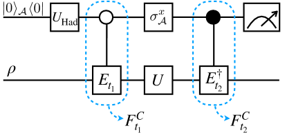
As pictorially represented in Fig. 1, the working principle of the scheme is to initialize the auxiliary system in the state where we denote with the eigenstates of the Pauli matrix for the auxiliary system (). We then perform a Ramsey interferometric scheme on [76, 77]. Between the application of both the Hadamard and gates, and the final projective measurement of (with respect to the observables , ), the auxiliary system interacts with the quantum system via the conditional (C) gates
| (48) | |||||
| (49) |
where
| (50) |
can be thought of as unitary evolution operators corresponding to the effective Hamiltonian for a time . Moreover, between the two conditional gates and , the quantum system undergoes the actual unitary dynamics of the process ruled by the evolution operator .
III.3 Detector-assisted measurement of quasiprobabilities
Here we provide a more general framework for the measurement of quasiprobabilities considering a quantum model for a detector coupled to the system of interest. This approach extends the TPM and the Ramsey scheme, by realising that the observation of the change of an observable can be attained not through von Neumann projective measurements, but rather via a generalized measurement or, more precisely, a positive operator-valued measure (POVM). This was first introduced by Roncaglia et al. in Ref. [38] to assess the thermodynamic work done on a quantum system (see Sec. IV), while a proposal for its measurement in cold atoms was reported immediately after in Ref. [39]. Moreover, an experimental realization of the POVM to measure quantum work done on a Bose-Einstein condensate is in Ref. [41]. In a series of papers, Solinas and his collaborators formalised this approach establishing a profound connection between fluctuations of quantum observables, quasiprobabilities and the full counting statistics [56, 19, 40, 42, 21].
We will describe two possible schemes: one that provides access to the characteristic function of the observable change , and the other providing directly the TPM probability distribution [19].
Let us imagine a system coupled to a detector that is modelled as a quantum free particle moving in one dimension. The detector is described by the canonical position and momentum operators. We assume that the system-detector interaction Hamiltonian is
| (54) |
where the time-dependent coupling constant is such that the detector is impulsively coupled to the system only at times and with strength . The operator is the observable to be measured and, without loss of generality, can be thought of being at time and at time , as formalized in Sec. II.
In the same spirit of what we discussed above, we consider the initial state of the system to be and that of the detector to be pure, i.e.,
| (55) |
where are eigenstates of the momentum operator with eigenvalue and is the initial momentum distribution of the detector. Moreover, for simplicity, let us assume the system to evolve with the unitary operator between times and . The extension to the case of a non unitary evolution described by a CPTP map is straightforward. The detector may also evolve during these times, but the effect of this free evolution can be very small or compensated, and we will therefore ignore it [19].
The final state of the detector, after tracing out the state of the system, can be cast in the following two equivalent forms, with [see Eq. (37)]:
| (56) | |||||
| (57) |
where we have used the expression of the NDQP, see Eq. (29). The last two equations are written in the detector momentum and position representations respectively, and we have introduced the detector position distribution as the Fourier transform of .
Some considerations are in order: since the detector momentum is a conserved quantity (as it commutes with the interaction Hamiltonian), the sole effect of the evolution is to induce phase shifts in the momentum eigenstates . By measuring these phase shifts we access information about the observable change . On the other hand, the evolution operator associated with the system-detector interaction is effectively a translation or displacement operator of the detector position. Therefore, the quantities can be also observed by measuring the detector position distribution. In the following, we will describe two schemes that follow these two ideas, respectively.
In the first scheme, the detector is initially prepared in a superposition of two states with opposite momenta of magnitude :
| (58) |
where is a real normalization constant 333If the states are the infinitely localised eigenstates of the detector momentum operator , the state is not normalizable. However, we can assume that are normalized narrow wave-packets with negligible overlap, in which case .. This corresponds to a momentum distribution . After the evolution, the state of the detector can be written as
| (59) |
where information about the dynamics is contained in the phase given that P is a conserved quantity (see also considerations above). If we now measure the phase accumulated during the whole evolution between the eigenstates and , we have access to a modified characteristic function:
| (60) | |||||
which resembles the characteristic function defined in Eq. (40), but this time computed over the NDQP of Eq. (29). Hence, to all effects, Eq. (60) represents the characteristic function of a non-demolition quasiprobability distribution. As already outlined at the level of quasiprobabilities in Sec. II.3.2, is a symmetric version of a KDQ characteristic function, where the symmetrization is done over the indexes and labelling the outcomes of the initial observable . Thus, the inverse Fourier transform of returns the NDQP distribution
| (61) |
that is real (since is real) but can assume negative values due to the non commutativity of and . When the initial state of the system does not have any coherence in the basis of eigenstates of , then for and the inverse Fourier transform of reduces to the TPM probability distribution, see Eq. (2).
In the second scheme, we analyze directly Eq. (57), which leads to the position probability distribution for the detector:
| (62) | |||
that is real and never negative as it derives from the expectation value of a Hermitian and positive semi-definite density operator. If we assume an initially localized detector position, , then
and Eq. (62) reduces to
| (63) |
that corresponds to the TPM probability distribution for . In contrast to the case in which is delocalised, in this case there is a unique relation connecting and allowing perfect reconstruction of the TPM probability distribition for from the statistics of the detector’s position .
Even though in Eq. (62) is real and positive semi-definite, effects due to initial quantum coherences can manifest themselves when the detector initial wave-function is not localized and has a width comparable or larger than the typical changes . In fact, imagine that , then in Eq. (62) the functions and may have an overlap that results in a modification of the position probability distribution if compared to the one provided by the TPM scheme.
III.4 Examples
We conclude this section by providing examples of the quasiprobability distributions obtained using the schemes presented above.
III.4.1 Weak-TPM scheme
Let us start with an application of the weak two-point measurement scheme to a three-level system (or a spin-) that is initialized in a generic density operator , and whose spin is consecutively measured along the orthogonal axes and . In particular, we take
that share the same set of eigenvalues , with eigenvectors
and
respectively. As in the qubit example in Sec. II.3.2, no quantum dynamics occurs in between the projective measurements of and i.e. . We now write the expression of the MHQ , the joint probability of the TPM scheme, the unperturbed final-time probability and the wTPM probability . We recall that can be all experimentally measured via a procedure based on single or sequential measurements. Moreover, by linearly combining them together according to Eq. (44), any MHQ can be fully reconstructed [12]. Thus, for the example under scrutiny,
| (64) | |||||
| (65) | |||||
| (66) |
and is given by Eq. (41) with and . In this example, are projectors with rank and describe the collapse of the spin-1 state onto a two-dimensional subspace. For completeness, the explicit expressions of with are:
Let us now take the initial density operator with
| (67) |
In the following, we provide the analytical expressions of , , and for a single pair : , . This choice ensures that . In doing this, we will show a specific example of how Eq. (44) effectively works:
| (68) |
From direct calculations, one can find that
Therefore,
| (69) | |||||
| (70) | |||||
| (71) |
Moreover,
| (72) | |||||
that validates Eq. (68).
III.4.2 Interferometric scheme
We consider the Ramsey interferometric scheme applied to a spin- particle that is sequentially measured along the and axis, as in the example reported in Sec. II.3.2. We recall that, in the case the initial density operator does not commute with , any procedure based on sequential projective measurements is invasive and unavoidably cancels out the quantum coherence contained in , with respect to the eigenbasis of . As a result, the statistics of the outcome pairs is distorted. The unperturbed statistics of the outcome pairs is provided by the KDQ distribution that, as shown in Sec. II.3.2, can exhibit negative and imaginary KDQ.
The interferometric scheme finds application to such a case-study by making the substitution , , and . In this way, by measuring the expectation values and , we can recover the real and imaginary parts of the KDQ characteristic function of the statistics of outcome pairs . In this case, the characteristic function reads as [see also Eq. (40)]
| (73) |
Using the initial state defined in Eq. (36), we obtain:
| (74) | |||||
such that the analytical expressions of the expectation values for the auxiliary system are
| (75) | |||||
Taking the inverse Fourier transform, we get the following QD for :
which may be complex depending on the form of .
It is instructive to point out that, by defining the effective Hamiltonian operators and , then Eq. (73) takes the more general expression
| (78) |
with . From this, we observe that the characteristic function of the KDQ distribution can be identically equal to the so-called Loschmidt [79, 80]. Hence, thanks to the link with the Loschmidt echo, and can be interpreted as the Hamiltonian operators governing, respectively, the forward and backward evolution of a perturbed quantum system 444In Eq. (78), the perturbation is introduced in considering two different Hamiltonian operators for the forward and backward dynamics that return the Loschmidt echo., and as the time instant at which the reversal operation takes place.
In Sec. V.2 we will show that the connection between the characteristic function of a KDQ distribution and Loschmidt echos does not hold only in specific examples, but it is valid in general for any quantum system. In this respect, condensed-matter physics and quasiprobabilities are deeply related.
III.4.3 Detector-assisted scheme
Let us consider the modified characteristic function in Eq. (60). Thus, by choosing the initial state qubit to be Eq. (36) as in III.4.2, we find:
| (79) |
which clearly depends on the presence of the off-diagonal element of the system density matrix .
Consequently, taking the Fourier transform we obtain the NDQP:
| (80) | |||||
that contains peaks at that are absent in the KDQ (or for an incoherent initial state) and that can be negative depending on the sign of . Another difference with the KDQ extracted from the Ramsey scheme, Eq. (III.4.2), is that Eq. (80) is strictly real.
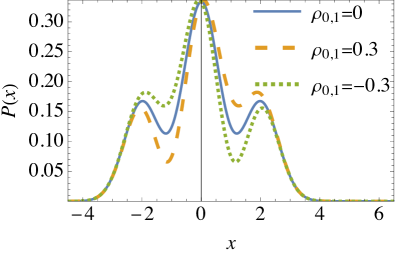
Let us now consider the signal observed in the position representation of the detector assuming for concreteness the detector’s wave-function , albeit any localized function would be suitable. From Eq. (62), we obtain , where the incoherent and coherent parts of the distributions read:
| (81) | |||||
The probability density would always appear in the expression of , even in the absence of initial coherence. It represents a coarse grained version of the TPM probability distribution; see Eq. (39) for the general definition. On the other hand, is proportional to and can be negative (although can never be negative).
We show in Fig. 2 and compare the cases when and . The latter case brings an asymmetry to the function and for sufficiently large a shift in the position of the peaks.
IV Quantum thermodynamics
In Sec. II, we have argued that, in the general case of and arbitrary non-commuting operators, the first measurement of the TPM scheme is invasive. Specifically, the TPM scheme does not allow one to recover the unperturbed single-time probability by marginalizing the joint probability of the TPM scheme over the outcomes of the first measurement. As a result, applying the TPM scheme breaks the no-signaling in time condition, failing to capture non-commutativity in the statistics of the measurement outcomes taken at times and [5, 20]. This evidence is proven to be true for arbitrary quantum observables and . Consequently, the same considerations shall hold in a thermodynamic context, where the measured observables are Hamiltonian operators.
Kirkwood-Dirac quasiprobabilities can be employed to investigate non-classical energetic processes, where here ‘non-classical’ indicates the presence of negative and imaginary values in the quasiprobability distribution of the thermodynamic quantity of interest, for instance, work, heat or entropy. In the current literature, Margenau-Hill quasiprobability distributions [82, 30, 5, 8, 12, 83], the real parts of Kirkwood-Dirac ones, have been already discussed and employed to characterize non-classical work distributions [84, 12], as well as the statistics of anomalous heat exchanges due to quantum correlations [8].
In this section, we discuss the KDQ approach to characterize the statistics of internal energy fluctuations in a generic quantum system, close or open. Then, we will focus on the ways the presence of non-classicality is responsible for anomalous energy exchanges [22] (see below for a proper definition) that can be identified, e.g., in the average and variance of work and heat distributions.
As we are going to show in Sec. IV.4, negative probabilities in a KDQ distribution of work find an interpretation as non-classical energy transitions that make use of quantum coherence to transform absorbed energy in extractable work. In this regard, we will show how KDQ can take into account genuinely quantum features in energy-change fluctuations, and outline thermodynamic advantages. For example, this becomes evident when noting that, without quantum coherence, stochastic work processes can generate a lower amount of extractable work and thus be less performing in operating a quantum device.
IV.1 Quantum internal energy distribution
From a stochastic thermodynamic point of view, any internal energy difference of a quantum transformation is a stochastic process. This holds even for isolated systems, since energy-change fluctuations—that however average to zero—are induced by the measurement apparatus. We recall that the latter irreversibly perturbs the measured (thermodynamic) system in any sequential measurement procedure that is directly performed on the system.
In the following, we are going to introduce the concepts of stochastic internal energy and stochastic quantum work in a generic quantum scenario with arbitrary density operators and time-dependent thermodynamic transformations. Let us identify the time-dependent quantum observables and with the Hamiltonian operators and at the initial and final times of the transformation under scrutiny. The Hamiltonian operators admit the spectral decomposition:
| (83) | |||||
| (84) |
where denote the indexes on the initial and final energies, respectively. From Eqs. (83)-(84), the definition of the stochastic internal energy follows. is defined within the time interval , and it is given by the differences . Notice that depends only on the eigenvalues of the Hamiltonian at the initial and final times of the thermodynamic transformation described by the CPTP map which the system is subject to, and not directly on itself. On the other hand, what is dependent on is the probability distribution ruling the occurrence of any value of . Thus, in order to describe such a distribution, we introduce the Kirkwood-Dirac quasiprobability defined as
| (85) |
with the initial density operator, such that the quasiprobability distribution of is
| (86) |
Notice that, from here on, we are going to use a simplified notation for the KDQ, using as a subscript the labels for the initial and final energies, respectively.
Following what we previously stated in Sec. II.3 about the properties of a KDQ, all the information about the statistics of the stochastic internal energy is also contained in the characteristic function
| (87) |
obtained by the Fourier transform of . As such, the KDQ distribution of the internal energy variation can be directly evaluated by means of the interferometric schemes discussed in Sec. III.2. As in the general case, the characteristic function —as well as each KDQ —is formally a quantum correlation function that takes the form
| (88) | |||||
For the case of time-dependent unitary dynamics (possibly leading to work fluctuations),
| (89) |
where is the evolution of the Hamiltonian of the quantum system at the final time of the work protocol in the Heisenberg picture.
It is worth also stressing that, when or , the corresponding KDQ can be a complex number, with possibly a negative real part. We recall that we have denoted this circumstance as being non-classical. Even in this quantum thermodynamics case, the non-classicality of the internal energy distribution , in the time interval , is measured via the functional computed over the KDQ .
IV.2 Quantum work & KDQ correction to Jarzynski equality
In any closed quantum system that is driven by a time-dependent Hamiltonian in the time interval , the internal energy difference corresponds to the exerted work . This means that , being the dissipated heat equal to zero in such a case.
In the context of (quantum) work fluctuations, the Jarzynski equality (JE) [85, 32]
| (90) |
with labelling the -th realization of the work protocol, is a cornerstone result in non-equilibrium statistical physics. In fact, Eq. (90) relates a fluctuating physical quantity (the work ) measured for an out-of-equilibrium system in a given time during the work protocol, and the equilibrium free-energy difference
| (91) |
where is the system partition function in equilibrium at inverse temperature with the Hamiltonian . Notice that setting the limit of ensures the overcoming of all convergence issues [86, 87, 88], and the direct connection with the average of the energy differences over all the statistical configurations dictated by the corresponding work distribution. For practical purposes, the value of can be taken finite but sufficiently large.
The equilibrium free-energy difference is achieved asymptotically by the driven quantum system under the assumptions that, once the work protocol is over, (i) the Hamiltonian of the system is assumed constant and equal to ; (ii) the system is put in contact with a thermal bath at inverse temperature . Moreover, in Eqs. (90)-(91), it is implicitly assumed that the quantum system is connected to the thermal bath at inverse temperature also before the work protocol is applied.
As surveyed in Ref. [89, 90, 91, 92], the symmetries allowing for the JE in Eq. (90) to hold are generally maintained as long as (I) the initial density operator is thermal at inverse temperature , namely ; (II) the dynamics of the quantum system is unital, meaning that the identity is a fixed-point of the quantum map to which the system is subject: . Notice that unitary dynamics are a subgroup of such more general family of maps. Therefore, a requirement for the validity of the JE is that is a thermal state, i.e., both (a) , and (b) the diagonal elements of (with respect to the eigenbasis of ) follow a Boltzmann distribution.
As a result, the JE in Eq. (90) can be obtained by applying the TPM scheme, which returns the following characteristic function for any given work distribution:
| (92) | |||||
with the joint probabilities of the TPM scheme, and complex number. Hence, by setting , we get
| (93) |
This simple derivation singles-out that, under the limit of , the average over the realizations of the work protocol is identically equal to the statistical average with respect to the work distribution returned by the TPM scheme. Moreover, if one applies the Jensen inequality on both sides of Eq. (93), we directly get the inequality
| (94) |
that is one of the formulation of the second law of thermodynamics in relation with the Clausius theorem.
Let us now start connecting these results with the discussion undertaken in the previous sections. In this regard, we already know from Sec. II that, if the density operator at the beginning of the work protocol does not contain quantum coherence with respect to the eigenbasis of (), then the first energy measurement of the TPM scheme is not invasive. Hence, in such a case, denotes, without any ambiguities, the dissipated work that is the amount of work that cannot be converted in extracted work.
However, the JE breaks down if is not a thermal state. The failure of the JE also occurs when is thermal but the dynamics of the quantum system is non-unital, possibly leading to heat dissipation [93, 94, 95, 96]. As a consequence, one ends up with an expression similar to the JE that exhibits a correction that is not a state function and depends on both the dynamical map to which the quantum system is subject and its initial state. We stress that this holds also in the case no quantum coherence is contained in , i.e., . Accordingly, by setting , the characteristic function of the work distribution provided by the TPM scheme reads as [97, 98, 99, 100, 101]
| (95) |
where
| (96) |
with and for work protocols. Being expressed as a function of the dynamical transformation applied to the system, the efficacy depends on the time , making generally a time-dependent quantity. Of course, if and is a unital map. We recall that the difference is commonly known as athermality as it quantifies the non-thermal contributions in the diagonal of with respect to the eigenbasis of . The athermality can be a significant thermodynamic resource if the quantum system undergoes dynamics with feedback [102, 103, 101].
If we now abandon the use of the TPM scheme and work in the more general framework of a quasiprobability distribution, how is the average exponentiated work modified if , namely quantum coherences are present in the initial density operator ? It is indeed clear that, since is not thermal, the JE in Eq. (90) is no longer valid and a further correction has to be included to attain a modified JE expression even for this case. Notice that a different correction has to be considered for all the protocols that go beyond the TPM scheme [104, 105, 67, 106].
The use of KDQ to describe quantum work fluctuations leads to the relation
| (97) | |||
| (98) |
is the KDQ correction to the JE that holds for any CPTP map . In conformity with the results shown in Sec. II, when , i.e., under the commutative condition . Similar to the efficacy , the KDQ-correction to the JE is not a state function, and therefore depends on the specific thermodynamic transformation that is performed on the system. However, in contrast to the TPM result, is in general a complex number, whose real part can take both negative and positive values. Consequently, as a possible application, if one measured or , it would imply the presence of non-classicality, since the non-positivity function in Eq. (25) would necessarily be greater than zero.
We conclude this subsection by admitting that the thermodynamic meaning of the KDQ-correction , as well as the corrections for the other protocols beyond the TPM scheme, is still lacking, meaning that further investigations are thus needed.
IV.3 Non-classical work exerted by qubits: A case-study
In this section, we discuss a simple example to analyze the KDQ distribution of work done on a single qubit that is driven by a work protocol described by a unitary operator . Assuming the system does not interact with any external bath, the internal energy change can be fully identified as work. Albeit simple, this model can be solved analytically and finds experimental applications in nuclear magnetic resonance (NMR) spin systems [106] and nitrogen-vacancy (NV) centers [68, 12] (point defects in the diamond lattice), where experiments of quantum thermodynamics beyond TPM have been recently performed.
Let us assume the Hamiltonian of the qubit to be:
| (99) |
corresponding to a spin-1/2 particle subject to an effective magnetic field rotating around the -axis. In the rotating frame, described by the unitary operator , the effective Hamiltonian describing the dynamics of the qubit becomes time-independent and reads
| (100) |
so that the system’s evolution operator (in the original frame) is
| (101) |
To find the statistics of work done between times and , we use the spectral decomposition of the time-dependent Hamiltonian, i.e.,
| (102) | |||||
| (103) | |||||
| (104) |
where we have defined a generalized Rabi frequency . Moreover, we assume the system to have quantum coherence in the eigenbasis of , so that
| (105) |
where corresponds to the populations of the initial eigenstates, and is the quantum coherence that we have chosen to be real for simplicity. Using the definition of the quasiprobability distribution for work, see Eq. (86), we find:
| (106) | |||||
where the KDQ are [see Eq. (85)]:
| (107) | |||||
| (108) | |||||
| (109) | |||||
| (110) |
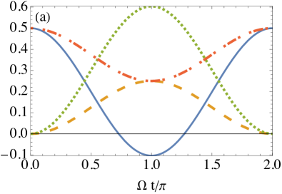
First, we notice that the imaginary parts of are always proportional to the coherence . Second, the real parts of may become negative. To see this, we specify, for simplicity, initial conditions and take the maximum possible coherence: . In this case, the real parts become:
| (111) | |||||
| (112) | |||||
| (113) | |||||
| (114) |
It is possible to see that the minimum value of is that is obtained for . Similarly, the minimum value of is also attained for . The time-dependence of the quasiprobabilities is shown in Fig. 3 for the two cases . It is interesting to see that only one of the may become negative for each value of . Moreover, choosing complex may lead to another of the to become negative, but the minimum value is still .
IV.4 Enhancement of extractable work
In this section, we are going to explain the meaning of non-classical work extraction and anomalous energy exchange or variation.
In any system that is subject to a work protocol, the extractable work is defined as the amount of energy that is left over, with respect to the energy of the system at the beginning of the transformation. Accordingly, if a protocol admits non zero extractable work, then the average energy at the end of the work protocol, , is smaller than the average energy at the beginning, , so that the extra energy amount can be used by a work reservoir [107] or stored in a battery [108]. Hence, the requirement for work extraction is that
| (115) |
Recently, it has been discussed whether the negativity of the terms composing a quasiprobability work distribution may correspond to an enhancement of work extraction, and whether this circumstance can be witnessed by violating an inequality that is instead valid under the commutative conditions and , i.e., when . The answer to both these questions is positive [12].
In order to see this, at the level of energy transitions, let us consider the fact that an excitation process (indexes , labelling the initial and final energies, respectively) occurring in a quantum process with negative quasiprobability is equivalent to a de-excitation process in a classical work transformation with probability .
During an excitation (stochastic) process, the system absorbs energy and uses this energy to carry out a transition between the energy levels. On the other hand, any de-excitation process that is operated by a thermodynamic transformation contributes to increase the amount of the extractable work. Therefore, the presence of negative quasiprobabilities can be effectively exploited as a resource to enhance work extraction, beyond what any classical stochastic process can achieve. Such enhancement is deemed as ‘non-classical’, and the internal energy variations associated to negative probabilities, enabling it, are called ‘anomalous’. Thus, anomalous energy variations denote energy exchanges that are inherently quantum mechanical, and heralded by the non-positivity of KDQ.
Let us see how the enhancement of work extraction occurs. If one uses the TPM scheme, the work extraction is maximized if we minimize . Without specifying anything about the thermodynamic transformation, the necessary condition to achieve the largest extractable work is to set
| (116) |
such that
| (117) |
leads to extractable work (in absolute value) in the TPM framework.
If instead the statistics of the internal energy variations are described by quasiprobabilities (for example when , as shown in Sec. II), then the extractable work can be enhanced beyond what is obtained by the TPM scheme, by setting
| (118) |
In this way, the magnitude of the extractable work
| (119) |
can be effectively maximized and satisfies the inequality
| (120) |
To achieve this, any excitation process has to be associated to a negative , while any de-excitation process should occur with positive quasiprobability. It is worth observing that for the task of work extraction, the imaginary parts of KDQ do not play an effective role, since they do not affect the average work. Also notice that enhanced extractable work, enabled by negativity, can be experimentally demonstrated, not by means of a procedure based on sequential measurements, but via a procedure that is able to reconstruct KDQ [see Sec. III].
What really matters to get enhanced work extraction is to ensure non-classical behaviours in the time-distribution of negativity, namely the distribution over time of the quasiprobabilities with negative real part. In fact, it is not crucial for the non-positivity functional to take a large value, but that a significant negativity is associated to a positive ‘anomalous’ energy variations . At the same time, work extraction is enhanced when negative values of occur with the largest possible positive quasiprobability . The interplay of all these conditions is model-dependent and depends on the specific parameters that rule the dynamics of the work process. Therefore, it is evident that attaining enhanced work extraction stems from an optimization routine that makes Eqs. (118) valid in a given time interval of the work protocol.
In Ref. [12], the electronic spin of an NV center in bulk diamond at room temperature was considered as the system to which a work protocol would be applied. Work extraction was observed and its maximum values were associated to negative fulfilling Eq. (120). The work extraction enhancement observed in Ref. [12] originates from a sub-optimal solution for the optimization of work extraction against the time duration of the work protocol. In fact, due to the experimental constraints, only one internal energy change , corresponding to the largest possible value, was associated with a negative quasiprobability. At the same time, the smaller internal energy variation occurred with positive quasiprobability, with all other quasiprobabilities being negligible.
IV.4.1 Enhanced extractable work from violating a classical inequality
We are going to show that fulfilling Eq. (120) implies the violation of an inequality for work extraction that holds as long as the commutativity condition is obeyed [12]. The violation of such an inequality cannot occur in any experiment implementing the TPM scheme.
Let us thus consider that the projectors and of the Hamiltonian at the initial and final times and of the work protocol are rank 1 operators. This means that and . Moreover, we assume, for simplicity, the initial density operator to be pure. Under these assumptions, the MHQ takes the form
| (121) |
Interestingly, all the terms , , are complex numbers whose real parts are linked with a standard probability amplitude, either defined at a single time or measurable by means of the TPM scheme. In particular, for the probability to measure the initial energy of the system, one has
| (122) |
where is a phase factor. Then, in the same spirit, we can write
| (123) |
and
| (124) |
where are the corresponding phase factors.
In Eq. (123), is the conditional probability (associated to the TPM scheme) of measuring the energy at time conditioned to have measured at time . Instead, in Eq. (124), is the probability to measure the energy at the end of the work protocol, by initializing the system in . Notice that, by construction, the probability encodes information on the quantum coherence that is initially present in ; for this reason, is a key element of the EPM scheme [67, 68, 109].
Overall, combining Eqs. (122)-(124) we arrive at
| (125) |
where, by definition, is the joint probability returned by the TPM scheme, and that is named activity [12]. The latter brings information on the quantum interference fringes among the eigenbasis of , and . It is indeed the activity that is responsible for the negativity of , such that if and only if .
If we substitute Eq. (125) into the expression of the work extraction, we find
| (126) |
whenever . The inequality in Eq. (126) gives an upper bound, dependent on the work protocol, to the amount of extractable work when , and applies also to initial mixed quantum states. Hence, a violation of this bound, as experimentally tested in Ref. [12], is a witness of the presence of negativity, as well as non-classical work extraction.
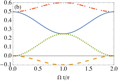
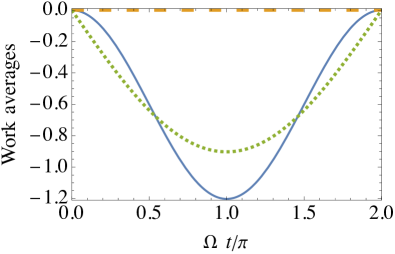
In Fig. 4, we show an example of the enhancement of work extraction aided by negativity in the qubit driven work protocol introduced in IV.3. In particular, we plot the average work of the TPM and KDQ probability distribution using the energies and Hamiltonian projectors in Eqs. (103)-(104), as well as the quasiprobabilities in Eqs. (107)-(110), with , ( to get the work statistics of the TPM scheme), and .
Interestingly, if the initial state of the qubit [see Eq. (105)] is fully mixed (), then the average work is zero for any value of the final time , see Fig. 4. On the other hand, turning on the quantum coherence in and making use of quasiprobability to attain the work distribution , the energy injected by the driving field is transformed into extractable work, beyond the classical bound [right-hand-side of Eq. (126)] in the interval approximately.
IV.5 Work variance in the KDQ setting
In the previous section, we have shown how using KDQ to describe the work fluctuations makes the average work equal to the corresponding value that is unperturbed by the measurement disturbance. Moreover, even though the KDQ are complex numbers, the average work is always a real number, with a clear interpretation with classical physics, as shown above.
In the following, we analyze how the fact that are complex numbers affects the second moment of the KDQ distribution of work, , i.e., the work variance . This is formally defined by
| (127) | |||||
where, as before, all the averages are performed with respect to , and the second statistical moment reads as
The quantity in the right-hand-side of Eq. (IV.5) is a two-time quantum correlation function for the Hamiltonian and is generally complex, making also complex. This means that the imaginary part of is equal to the imaginary part of , whose meaning lies in the presence of phase correlations in the scalar products of the eigenvectors of and at the times . For this reason, the quantum correlation function for preserves information about the quantum coherence contained in , and this feature is transferred to the work variance . In this regard, we are going to show that the imaginary part of , , is directly linked with the non-commutativity between and . From this, following the time-energy Schrödinger-Robertson uncertainty relation [110, 111, 112], is bounded by the product of the uncertainties of and respectively.
A first expression of the work variance is obtained by combining Eqs. (127)-(IV.5), so that:
where
| (130) |
and
| (131) |
The last term in the right-hand-side of (IV.5) identifies the way Hamiltonian operators at distinct times correlate in a quantum work protocol. The real and imaginary parts of are equal respectively to 555For any density operator and two quantum observables and , one can split the trace into real and imaginary parts: .:
| (132) |
and
| (133) |
Eq. (IV.5) defines the quantum covariance of and . Instead, in Eq. (IV.5) is a purely imaginary number and, by definition, is the expectation value of the commutator with respect to the initial density operator .
This derivation demonstrates that the work variance has both a real and an imaginary part. The real part has a clear correspondence with the thermodynamics of classical systems, as
| (134) | |||||
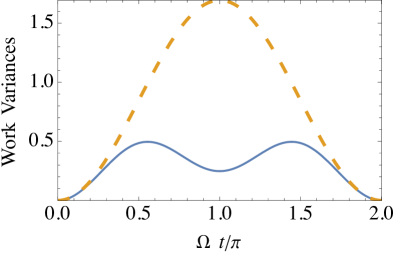
In addition, the fact that the commutator or may lead to a decreased work variance, namely to . We show this for the driven qubit of Sec. IV.3 and report the results in Fig. 5 where we assume the same values used for Fig. 4. Interestingly, apart for where both the work average and variances are zero, the real part of the KDQ work variance has a local minimum at that is the time instant with maximum negativity.
On the other hand, the imaginary part of the work variance is
| (135) |
that quantifies the possible non-commutativity of and . The magnitude of can be upper bounded by making use of the time-energy Schrödinger-Robertson uncertainty relation [110, 111, 112]. In fact, the latter states that, for any quantum observables , and density operator ,
| (136) |
where and
| (137) |
with . Therefore, by applying the inequality in Eq. (136) to our setting, we obtain the inequality
| (138) |
IV.6 Heat fluctuations in the quantum regime
In this section, we no longer deal with work distributions, and we will focus on heat fluctuations. For this purpose, we consider the paradigmatic model that consists in placing into contact a cold and a hot quantum system, which globally undergo a unitary quantum dynamics. Depending on the initial quantum states of the cold and hot systems, different results as well as thermodynamic interpretations can be drawn. In this context, a first relevant result is in Ref. [114] and goes under the name of Jarzynski-Wójcik exchange fluctuation theorem. In Ref. [114], two quantum systems and with finite Hilbert space dimension are prepared in two equilibrium thermal states at different temperatures and with . Then, they are made weakly interacting with one another for a given time interval. Under this assumption, one gets that
| (139) |
where is the stochastic heat exchanged by the two bodies, and denotes the difference of the inverse temperature of the initial thermal states for the two bodies.
If the initial global state of the two systems is a product state then the average in Eq. (139) can be performed with respect to the TPM distribution of the exchanged heat. To find this, it is sufficient to measure the statistics of the time-independent Hermitian operator represented by the sum of the local Hamiltonian operators of the two bodies, i.e., . Furthermore, throughout this section, we also implicitly assume the energy-preserving condition for the unitary operator that describes the quantum dynamics of the two bodies:
| (140) |
Eq. (140) physically entails that, at any time , the average energy variation in a body is minus the corresponding average energy variation in the other body. Such symmetry allows one to study fluctuations of exchanged energy between the two bodies by just measuring one of them.
In the literature, it has been considered also the case of an initial quantum state that is locally thermal as in [114], but also classically correlated [115]. This kind of correlations makes non-thermal the diagonal of the initial density operator for the two bodies taken individually, but does not add off-diagonal elements in with respect to . As shown in Ref. [115], a generalized exchange fluctuation relation, extending Eq. (139), can be still obtained, as we will discuss next.
Let us now introduce the spectral decomposition of the local Hamiltonians and for each of the two bodies:
| (141) |
with and . This implies that the projectors of the total Hamiltonian are .
For the initial state , we require that the reduced states of the each body is in equilibrium at inverse temperature :
| (142) | |||||
| (143) |
where are the local partition functions. We hence have: . While the reduced states are diagonal in the eigenbasis of , in general the global state may contain off-diagonal elements, with respect to the local energy eigenbasis, that may be the signature of the presence of quantum correlations.
We are now in the position to define the average heat flow that, due to the energy-preserving condition, can be inferred from the energy change of either the cold or the hot body. Without loss of generality, we choose to measure it for the cold system as in Ref. [8]. The average heat flow at the final time of the thermodynamic transformation is
| (144) |
where denotes the evolved density operator of the two bodies.
According to Eq. (144), denotes that heat flowing on average from the hot to the cold body, as naturally requested by the second law of thermodynamics with the intervention of no external drive. On the other hand, by resorting to additional resources, it can also occur that meaning that on average heat flows from the cold body to the hot one, as in a refrigerator. Summarising,
Moreover, if the amount of exchanged heat from the cold to the hot body exceeds in magnitude the value of , with the Hilbert space dimension of each body, then the heat backflows are called strong. Notably, the observation of strong backflows indicates that the actual quantum states of the bipartite system, on which heat fluctuations are evaluated, is entangled [116].
Let us introduce the quasiprobabilities associated to the energy variations , eigenvalues of the total Hamiltonian of the two bodies. Using again the definition of the quasiprobability distribution in Eq. (86), one has that
| (145) |
where and
| (146) |
is the corresponding joint probabilities returned by the TPM scheme. As before, in Eq. (146) we have employed the dephasing operator . In Eqs. (145)-(146) the initial quantum state of the two bodies is linearly decomposed as [see Eq. (5)], where both the diagonal and off-diagonal parts of are considered with respect to the eigenbasis of .
Based on this framework, we describe an exchange fluctuation relation that is also valid in the non-commutative regime of , due to the presence of quantum correlations or entanglement in the initial state. For this purpose, let us introduce the stochastic mutual information with elements
| (147) |
where , such that . We also recall that the energy variation in the cold body is , assuming the energy-preserving condition for and a resonant interactions between the bodies. Hence, we find [8]
| (148) |
where the average in Eq. (148) is made with respect to the quasiprobabilities , and
| (149) |
The correction to the exchange fluctuation theorem, , is equal to zero if , which is equivalent to and . In this case the application of the TPM scheme suffices. The exchange fluctuation relation Eq. (148) reduces to the Jarzynski-Wójcik identity Eq. (139) in the case , whereby . Instead, if the diagonal elements of are not thermally distributed—due to classical correlations in the eigenbasis—and , then one recovers the exchange fluctuation relation in [115], i.e.,
| (150) |
We conclude this theoretical analysis about heat fluctuations in the quantum regime, by providing the thermodynamic interpretation of the fluctuation profiles associated to the quasiprobability distribution of heat exchanges. Previously, we have seen that the presence of quantum correlations in the initial state can enhance the amount of heat backflows, such that according to the used convention. The explanation of this phenomenon lies in the possibility to associate negative quasiprobabilities to positive heat exchanges corresponding to heat flowing from the cold body to the hot one. Such a process, which needs an external energy source for its activation, is triggered by quantum correlations.
Notice that, in order for quantum correlations to be effectively considered as a resource for heat backflows, it is required that negative heat exchanges (i.e., energy fluxes from the hot to the cold bodies) occur with positive quasiprobabilities , similarly to what happens to work extraction in Sec. IV.4. When the enhancement induced by quantum correlations in allows for strong cold-hot heat backflows, then one can state that the corresponding energy exchange process takes non-classical traits.
IV.6.1 Example: Two-qubit system
We now apply the theoretical framework introduced above to a pair of interacting qubits, at inverse temperatures and , respectively, and local Hamiltonians . The two qubits are initialized in a global state containing off-diagonal elements with respect to .
As proven in [8], a general form of the initial state for a two-qubit system fulfilling the requirements (142)-(143) is
| (151) |
where is a population term, (), , and such that . In Ref. [8], it is also shown that the energy-preserving condition [Eq. (140)] is responsible to set a minimal form for the unitary operator :
| (152) |
with , equivalent to a partial swap transformation. In the expression of in Eq. (152), it is implicitly assumed that the interaction between the two bodies is taken resonant, in order to optimize the dynamics of heat exchange with energy-preserving.
Under these assumptions, the analytical expression of the heat exchange (144) between the two bodies reads [8]
| (153) |
where
| (154) |
is the average heat flow obtained by applying the TPM scheme, or by setting (no quantum coherence) in Eq. (153). For any value of , and , it can be easily found that , which means no cold-to-hot heat backflows is possible. This is evident in Fig. 6 where we plot Eq. (153) against for and for for fixed . From the figure it can be observed that, for some values of , (cold-to-hot heat backflows) is possible when . The parameter also affects the magnitude of the heat exchanged between the cold and hot systems.
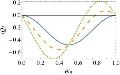
V Quantum many-body systems
Quasiprobability distributions play an instrumental role in the understanding of quantum many-body systems. In this section, we will present their applications in the context of quantum scrambling and out-of-time-ordered correlators (Sec. V.1), the Loschmidt echo (Sec. V.2) and a technique for efficiently calculating the quasiprobability distributions of free fermion systems (Sec. V.3).
V.1 Quantum scrambling & Out-of-time-ordered correlators (OTOCs)
Out-of-time-ordered correlators (OTOCs) allow the study of quantum information scrambling, a phenomenon in which localized quantum information rapidly spreads across multiple degrees of freedom in many-body systems [117, 118]. OTOCs have recently found extensive applications in diverse fields, such as condensed matter physics, quantum chaos, holography, and the study of black holes. Their versatility has thus pushed the development of numerous experimental proposals aimed at measuring OTOCs [119, 120, 121, 122, 123, 124], with some experiments already realized [125, 126, 127, 128, 129, 130].
In this section, we review the basic definition of OTOCs and show how they relate to quasiprobabilities. This connection has been recently noted in various works [131, 4, 23, 54].
Let us consider a system that is initially prepared at time in the state and subject to a time evolution described by the unitary operator . We also assume that, at the beginning of the dynamics, the system is perturbed by the application of a unitary operator 666Although in the OTOC literature, this is normally denoted as , we choose a different symbol to avoid confusion with the symbol for the work., acting locally on a part of the system. For instance©, if the system is made of qubits, we may consider the spin flip that acts on the qubit (see Fig. 7). As the system evolves in time, we would like to see how the dynamics of the perturbation affects the measurement of another local operator acting on another disjoint part of the system, e.g. with .
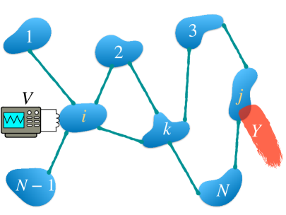
This can be assessed by considering the OTOC:
| (155) |
where, here and in the following, the average is always taken over the initial state : .
While the OTOC is in general a complex number, one can consider a real quantity by introducing the OTO commutator:
| (156) |
Its interpretation is quite clear: initially, the operators and commute as they have support on spatially separated parts of the system, . However, as time progresses, the effects of the perturbation may reach the support region of and their commutator might become nonzero: . The quantity measures the magnitude of this commutator. If both operators and are unitary, the OTO commutator is related to the OTOC by:
| (157) | |||||
Next, we are going to show that an OTOC is equal to the characteristic function of a KDQ. To this end, let us follow Ref. [133], which introduces the wing-flap protocol and express the unitary operator in exponential form in terms of its generator: with a Hermitian operator and a real scalar. The spectral decomposition of the observable reads: in terms of its real eigenvalues and the corresponding orthogonal projectors . Using these definitions, can be expressed as
| (158) |
Hence, we can define both the KDQ
| (159) |
and the change in the eigenvalues of when two measurements of are performed at times and , respectively. Notice that, in order to denote a quasiprobability, we continue using the simplified notation adopted in Sec. IV, whereby the subscript in contains the indexes labelling the measurement outcomes at the initial and final times of a two-time procedure. Then, the quasiprobability distribution to observe a change at time is given by
| (160) |
and the characteristic function of is its Fourier transform (see Sec. II.3.3), such that
| (161) | |||||
that can thus be expressed as an OTOC.
In general, whenever , both the KDQ and its characteristic function are complex numbers. When , the KDQ is real and positive, as explained in Sec. II.
Similar to Secs. II-IV, we can define the corresponding MHQ distribution that can be associated with an OTOC. Such a distribution is the real part of the corresponding KDQ one: and its characteristic function reads as
| (162) |
Interestingly, using the equality
| (163) | |||||
we obtain
| (164) |
Let us now consider a practical example and let
| (165) |
be the Hamiltonian of two qubits initially in the thermal state
| (166) |
with inverse temperature . Then, we choose and . Notice that neither nor commute with either or . Therefore, this is an ideal setting to test the possible presence of non-positivity in the KDQ (159). For this purpose, we can write the measurement observable as , from which and with the corresponding eigenvalues and . We stress that the projectors of act locally on qubit 2. One can see that the evolution operator is periodic with the frequency .
In Fig. 8, we show the real and imaginary part of fixing for various values of . It is evident that can become negative for sufficiently large and that is generally nonzero. We also show the quasiprobabilities . The negativity in is reflected in the negativity of the quasiprobability that is the only one becoming negative. Since the probabilities need to fulfil the normalization condition, it means that is amplified due to the presence of quantum coherences in the initial state , compared to a case in which the initial state commutes with the observable .
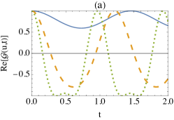
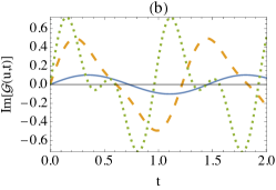
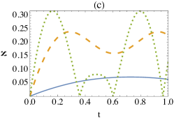
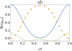
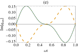
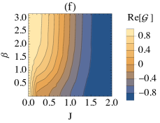
In Fig. 8(f), we show a contour plot of the minimum value of in the time interval as a function of and . First, as expected, we confirm that larger values of the interaction strength always lead to a stronger negativity. On the other hand, the effect of temperature is nontrivial, as increasing temperatures may lead to a larger negative value of . This seemingly counter-intuitive behaviour stems from the fact that sometimes initializing the quantum system in the ground state alone does not lead to non-positivity. Instead, the nonzero occupation of excited states, even if populated incoherently [134], and the transitions between them may lead indeed to negative quasiprobabilities. A similar behaviour is observed for the KDQ of the Ising model, see Sec. V.3.
V.2 Link with the Loschmidt echo
Another interesting connection of quasiprobability distributions with the irreversibility of many-body systems arises in the context of quantum chaos and decoherence. Consider a system of many particles, classical or quantum, that evolves in time for a period according to a time-independent Hamiltonian . If we were to invert all momenta and run the evolution backward we should be able to recover the initial state. However, little imperfections in the inverted evolution or decoherence induced by an external environment may cause some deviations. For an initial pure state , one can define the Loschmidt echo (LE) as the absolute square value of the complex amplitude
| (167) |
and the generalization to mixed states and non unitary evolutions is straightforward.
Mathematically, represents the fidelity, in terms of the overlap, between the initial state evolved with the unperturbed Hamiltonian and the state evolved with the perturbed Hamiltonian . Peres transferred the LE idea in the quantum domain [79], while Ref. [135] used the LE to analyze the decoherence of a many-body spin system and the relation to chaos. For the quantum version of systems with a classically chaotic Hamiltonian (for instance a particle moving in a driven double well, see Ref. [135]) the rate at which the information about the initial state is destroyed by the environment, within a range of couplings to the environment, is set by the classical maximal Lyapunov exponent. Under these assumptions, the LE decays exponentially in time with the Lyapunov exponent, thus revealing the underlying classical chaotic behaviour; see also Ref. [80].
Moreover, the LE was beneficial to uncover a new type of phase transition occurring in time. In this regard, if we assume that the initial state is the ground state of with zero energy, then the LE amplitude (167) reduces to
| (168) |
which looks like the partition function of the Hamiltonian but with an imaginary inverse temperature . Since classical phase transitions arise because of singularities in the partition function, Heyl and coworkers discovered dynamical quantum phase transitions as those that give rise to singularities in the LE at specific instants of time, see Refs. [136, 137].
The LE is also strongly connected with the statistics of work as mentioned in Sec. IV and described in detail in Ref. [138]. In fact, Eq. (167) can be interpreted as the characteristic function of the work done on a quantum system initially in the state , whose Hamiltonian is subject to a quench dynamics that instantaneously changes to .
Let us now formalize the connection between the LE and the KDQ. First, we write the spectral decomposition of the two Hamiltonian operators: and . With these assumptions, let us write an expression for the LE for a generic mixed initial state:
| (169) | |||||
where we have introduced the KDQ of the random variable , defined as
| (170) |
Thus, the Fourier transform of with respect to time , i.e.,
| (171) | |||||
can be interpreted as the quasiprobability distribution for the work done on the quantum system, which initially is in the state and whose Hamiltonian is suddenly changed from to . However, it is worth noting that in contrast to the characteristic function of work obtained using the TPM scheme [138], in the general case the initial state may not commute with any of the two Hamiltonian operators and . This fact, as we have seen in other examples earlier, may give rise to a distribution with non-positive values.
We now proceed to illustrate these concepts with a simple example. Let us consider a qubit in the pure initial state
| (172) |
and let us choose the Hamiltonian operators and as
| (173) | |||||
| (174) |
The eigenstates of are simply and , with eigenvalues respectively, and let us define the projectors on these states as with . Similarly, for , the eigenstates are:
| (175) | |||||
| (176) |
with eigenvalues , where we have introduced and the mixing angle such that
| (177) |
Hence, for the LE, we get:
| (178) |
whose real part is plotted in Fig. 9(a).
It is evident that for very small the two evolutions associated with and are very similar and remains close to 1. However, when increases, the perturbed Hamiltonian induces a diverging trajectory for the initial state . As the system is small, large revivals of the LE are possible for longer times, but the short time response is symptomatic of what would happen for a much larger system. Moreover, for the KDQ, we obtain:
| (179) |
where . After a close inspection, since , it is evident that that corresponds to the transition between the highest and the lowest energy eigenstates of and , respectively. Instead, all the other quasiprobabilities are strictly positive. They are plotted in Fig. 9(b). In the inset of the figure, we also plot the non-positivity functional , which is always nonzero (since one quasiprobability is always negative) and peaks around .
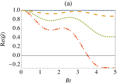
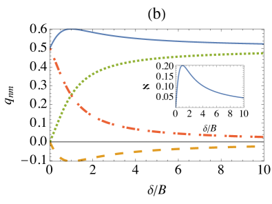
V.3 Quantum work in quadratic fermionic systems
In this section, we explain how to calculate the KDQ for systems of free fermions described by Hamiltonians that are quadratic in fermionic creation and annihilation operators. This is relevant not only for actual fermionic systems, for instance ultracold atoms in optical lattices, but also for systems that can be mapped onto free fermion models, for instance Ising and XY spin chains.
Quasiprobability distributions of work in quadratic fermionic systems have been recently calculated in a few references; see for instance Refs. [139, 16, 17]. Inspired by the approach taken in Ref. [139], here we showcase the calculation of the KDQ for an Ising spin chain with spin- particles, described by the Hamiltonian
| (180) |
where periodic boundary conditions are assumed: , . The parameter is an effective transverse magnetic field. The critical value separates the ferromagnetic phase, existing for , from the paramagnetic phase occurring for . Within the ferromagnetic phase, in the thermodynamic limit, the ground state is doubly degenerate with a macroscopic magnetization along , while in the paramagnetic phase the ground state is non degenerate and exhibits an induced magnetization along .
To diagonalize the Ising Hamiltonian in Eq. (180), following Refs. [140, 141], we first employ the Jordan-Wigner transformation that expresses the fermionic annihilation operators
| (181) |
in terms of the spin ladder operators .
Then, we transpose the problem to the quasimomentum space by defining the fermionic operators
| (182) |
where the possible values of the quasimomenta are with (assuming for simplicity even). Let us thus define the fermionic operators that are obtained by applying the following Bogoliubov rotation to the operators :
| (183) |
The fermionic operators depend on the angles , implicitly given by
| (184) |
and satisfy the canonical anti-commutation relations
| (185) |
In terms of the operators , the Hamiltonian Eq. (180) reduces to a diagonal form:
| (186) |
where
| (187) |
are the single particle eigenenergies.
In what follows, we consider a sudden change of the Hamiltonian in which the magnetic field is changed instantaneously from the initial value to the final value . To calculate the quasiprobabilities defined in Eq. (85), we need to express the fermionic operators , which diagonalize with eigenenergies , in terms of the fermionic operators diagonalizing with eigenenergies . This is possible thanks to the linear Bogoliubov transformation [140]:
| (188) |
where denotes the difference of Bogoliubov angles corresponding to , with . Let us now define the vacuum states and that are such that and . The vacua of the two Hamiltonian operators and are related by the relation
| (189) |
Here, the need for a quasiprobability approach arises whenever one chooses an initial state that has coherences in the eigenbasis of . In our example, we choose the following state:
| (190) |
with . In Eq. (190), is the Gibbs equilibrium thermal state that corresponds to the initial Hamiltonian, i.e.,
| (191) | |||
where is the inverse temperature, and is the total partition function, with denoting the partition function for each quasimomentum. Moreover, in Eq. (190), we have also introduced the coherent Gibbs state :
| (192) |
which has the same energy distribution of but is a pure state. Crucially, contains coherent terms in the initial energy eigenbasis, e.g., . This means that the initial state is a mixture of the Gibbs equilibrium state , which is diagonal in the eigenbasis of the initial Hamiltonian, and of that exhibits non diagonal quantum coherence.
Let us now calculate the KDQ distribution of the work done by suddenly change the Hamiltonian from to . Since , we can rewrite the initial state as:
From Eq. (189), we see that the eigenstates of with quasimomenta are transformed into the superposition of eigenstates of the with the same pair of quasimomenta. Therefore, we can compute the work done for all possible transitions from to that correspond to the work instances . The only transitions that have nonzero quasiprobabilities
| (193) |
are: where, for each process, we have included the value of the stochastic work instances and the associated quasiprobability. As expected, the quasiprobabilities with non vanishing work also depends on the mixture parameter , which weighs the contribution of the initial state containing quantum coherence in the eigenbasis of .
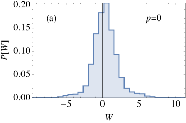
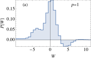
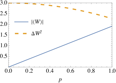
From the results above we can finally write the KDQ distribution of work by summing over all the quasimomenta :
| (194) | |||||
A coarse grained histogram of is shown in Fig. 10. For the distribution is always non-negative, while for some negative parts appear and are associated with positive values of . As a consequence , corresponding to work extraction, tends to be enhanced, so that , as explained in Sec. IV.4 and shown explicitly in Fig. 11. Notice that, in order for to exhibit negativity, the temperature entering must be high enough for two-body processes to be significant. In contrast, if the initial state is close to the ground state these processes are suppressed and is non negative everywhere. Initial state coherence also leads to a reduction of the work fluctuations as measured by its variance, see Fig. 11.
VI Discussion
Quasiprobabilities have been quite elusive quantities so far, due to the difficulty for their experimental inference. As stressed in Sec. II, procedures based on sequential projective measurements cannot reconstruct the quasiprobability distribution of a physical quantity that is defined over two times, as well as its corresponding statistical moments.
Recently, however, we have witnessed a resurgence of quasiprobabilities, thanks to their direct link with two-point quantum correlation functions of the form , with , quantum observables, and the average performed with respect to a generic density operator . Quantum correlation functions are a powerful tool to describe phase changes in quantum statistical mechanics. Hence, the possibility to express them in terms of quasiprobabilities opens the door for building a microscopic, nonequilibrium description of phenomena that naturally includes genuinely quantum resources as quantum coherence and correlations.
Beyond theoretical arguments, quasiprobabilities may turn out to be pivotal also for revealing advantages in quantum technology applications. In this tutorial we have seen several examples in quantum thermodynamic applications, particularly in experiments, including work extraction [12]. This is also relevant for the energetic assessment of quantum computation, where the energy exchange of a qubit with its environment can be continuously monitored through weak measurements [22].
The contextual nature of quantum systems facilitates the emergence of anomalous weak values of the energy exchanges due to quantum coherence which manifest themselves through negative quasiprobability distributions. In the context of metrological applications, negative values of quasiprobability distributions may enhance parameter estimation increasing the precision of quantum sensing protocols [7, 24].
We conclude the tutorial by mentioning some possible future perspectives of the topics treated here. By now, it should be apparent how quasiprobabilities have connections with all main theoretical and experimental aspects of quantum theory. Here, we explored the direct link with quantum measurement theory, fluctuation theorems, work and heat in quantum systems led by genuinely quantum resources, and the scrambling of information in many-body systems. Thus, further investigations on the following subjects could be considered:
-
(i)
To determine how the thermodynamic entropy production in a nonequilibrium quantum process is expressed in terms of a quasiprobability distribution. In doing this, one could determine the link with quantum information theory and feedback mechanism naturally including so-called Maxwell’s demons [142].
-
(ii)
The extension of two-time quasiprobability distribution to access multi-time statistics in open quantum systems. This could help investigating non-Markovian effects arising because of memory effects in the environment.
-
(iii)
To define to what extent the quasiprobability distribution underlying an OTOC can be a proper quantum sensing toolbox. In fact, given a quantum many-body system, different perturbations may scramble differently the state of the global system [130], and the corresponding quasiprobability distribution could give access to this information and measured by means of an interferometric procedure.
We hope that the curious and interested reader can find new, fascinating ideas from this tutorial, and can develop some of the perspectives listed here, by opening in turn further open problems.
Acknowledgements
We acknowledge enlightening discussions with Kenza Hammam, Paolo Solinas and Nicole Yunger-Halpern. SG acknowledges financial support from the project PRIN 2022 Quantum Reservoir Computing (QuReCo), the PNRR MUR project PE0000023-NQSTI financed by the European Union–Next Generation EU, the MISTI Global Seed Funds MIT-FVG Collaboration Grant “Revealing and exploiting quantumness via quasiprobabilities: from quantum thermodynamics to quantum sensing”, and the Royal Society project IES\R3\223086 “Dissipation-based quantum inference for out-of-equilibrium quantum many-body systems”. GDC acknowledges support from the UK EPSRC through Grants No. EP/S02994X/1.
References
- Spekkens [2008] R. W. Spekkens, Negativity and Contextuality are Equivalent Notions of Nonclassicality, Phys. Rev. Lett. 101, 020401 (2008).
- Ferrie [2011] C. Ferrie, Quasi-probability representations of quantum theory with applications to quantum information science, Rep. Prog. Phys. 74, 116001 (2011).
- Ryu et al. [2013] J. Ryu, J. Lim, S. Hong, and J. Lee, Operational quasiprobabilities for qudits, Phys. Rev. A 88, 052123 (2013).
- Yunger Halpern et al. [2018] N. Yunger Halpern, B. Swingle, and J. Dressel, Quasiprobability behind the out-of-time-ordered correlator, Phys. Rev. A 97, 042105 (2018).
- Lostaglio [2018] M. Lostaglio, Quantum Fluctuation Theorems, Contextuality, and Work Quasiprobabilities, Phys. Rev. Lett. 120, 040602 (2018).
- González Alonso et al. [2019a] J. R. González Alonso, N. Yunger Halpern, and J. Dressel, Out-of-Time-Ordered-Correlator Quasiprobabilities Robustly Witness Scrambling, Phys. Rev. Lett. 122, 040404 (2019a).
- Lostaglio [2020] M. Lostaglio, Certifying Quantum Signatures in Thermodynamics and Metrology via Contextuality of Quantum Linear Response, Phys. Rev. Lett. 125, 230603 (2020).
- Levy and Lostaglio [2020] A. Levy and M. Lostaglio, Quasiprobability Distribution for Heat Fluctuations in the Quantum Regime, PRX Quantum 1, 010309 (2020).
- Arvidsson-Shukur et al. [2021] D. R. M. Arvidsson-Shukur, J. Chevalier Drori, and N. Yunger Halpern, Conditions tighter than noncommutation needed for nonclassicality, J. Phys. A: Math. Theor. 54, 284001 (2021).
- De Bièvre [2021] S. De Bièvre, Complete Incompatibility, Support Uncertainty, and Kirkwood-Dirac Nonclassicality, Phys. Rev. Lett. 127, 190404 (2021).
- Lostaglio et al. [2023] M. Lostaglio, A. Belenchia, A. Levy, S. Hernández-Gómez, N. Fabbri, and S. Gherardini, Kirkwood-Dirac quasiprobability approach to the statistics of incompatible observables, Quantum 7, 1128 (2023).
- Hernández-Gómez et al. [2023a] S. Hernández-Gómez, S. Gherardini, A. Belenchia, M. Lostaglio, A. Levy, and N. Fabbri, Projective measurements can probe non-classical work extraction and time-correlations, arXiv preprint arXiv:2207.12960v2 10.48550/arXiv.2207.12960 (2023a).
- De Bièvre [2023] S. De Bièvre, Relating incompatibility, noncommutativity, uncertainty, and Kirkwood–Dirac nonclassicality, J. Math. Phys. 64, 022202 (2023).
- Zhang and Wang [2022] K. Zhang and J. Wang, Quasiprobability fluctuation theorem behind the spread of quantum information, arXiv preprint arXiv:2201.00385 10.48550/arXiv.2201.00385 (2022).
- Cerisola et al. [2023] F. Cerisola, F. Mayo, and A. J. Roncaglia, A Wigner Quasiprobability Distribution of Work, Entropy 25, 1439 (2023).
- Francica and Dell’Anna [2023] G. Francica and L. Dell’Anna, Quasiprobability distribution of work in the quantum Ising model, Phys. Rev. E 108, 014106 (2023).
- Santini et al. [2023] A. Santini, A. Solfanelli, S. Gherardini, and M. Collura, Work statistics, quantum signatures, and enhanced work extraction in quadratic fermionic models, Phys. Rev. B 108, 104308 (2023).
- Pratapsi et al. [2024] S. S. Pratapsi, S. Deffner, and S. Gherardini, Quantum speed limit for kirkwood-dirac quasiprobabilities, arXiv preprint arXiv:2402.07582 10.48550/arXiv.2402.07582 (2024).
- Solinas and Gasparinetti [2016] P. Solinas and S. Gasparinetti, Probing quantum interference effects in the work distribution, Phys. Rev. A 94, 052103 (2016).
- Beyer et al. [2022] K. Beyer, R. Uola, K. Luoma, and W. T. Strunz, Joint measurability in nonequilibrium quantum thermodynamics, Phys. Rev. E 106, L022101 (2022).
- Solinas et al. [2022] P. Solinas, M. Amico, and N. Zanghì, Quasiprobabilities of work and heat in an open quantum system, Phys. Rev. A 105, 032606 (2022).
- Maffei et al. [2023] M. Maffei, C. Elouard, B. O. Goes, B. Huard, A. N. Jordan, and A. Auffèves, Anomalous energy exchanges and Wigner-function negativities in a single-qubit gate, Phys. Rev. A 107, 023710 (2023).
- Dressel et al. [2018] J. Dressel, J. R. González Alonso, M. Waegell, and N. Yunger Halpern, Strengthening weak measurements of qubit out-of-time-order correlators, Phys. Rev. A 98, 012132 (2018).
- Lupu-Gladstein et al. [2022] N. Lupu-Gladstein, Y. B. Yilmaz, D. R. M. Arvidsson-Shukur, A. Brodutch, A. O. T. Pang, A. M. Steinberg, and N. Y. Halpern, Negative Quasiprobabilities Enhance Phase Estimation in Quantum-Optics Experiment, Phys. Rev. Lett. 128, 220504 (2022).
- Kirkwood [1933] J. G. Kirkwood, Quantum statistics of almost classical assemblies, Phys. Rev. 44, 31 (1933).
- Dirac [1945] P. A. M. Dirac, On the analogy between classical and quantum mechanics, Rev. Mod. Phys. 17, 195 (1945).
- Breuer and Petruccione [2002] H.-P. Breuer and F. Petruccione, The Theory of Open Quantum Systems (Oxford University Press on Demand, 2002).
- Caruso et al. [2014] F. Caruso, V. Giovannetti, C. Lupo, and S. Mancini, Quantum channels and memory effects, Rev. Mod. Phys. 86, 1203 (2014).
- Hofmann [2014] H. F. Hofmann, Sequential measurements of non-commuting observables with quantum controlled interactions, New J. Phys. 16, 063056 (2014).
- Halliwell [2016] J. J. Halliwell, Leggett-garg inequalities and no-signaling in time: A quasiprobability approach, Phys. Rev. A 93, 022123 (2016).
- Campisi et al. [2011] M. Campisi, P. Hänggi, and P. Talkner, Colloquium: Quantum fluctuation relations: Foundations and applications, Rev. Mod. Phys. 83, 771 (2011).
- Jarzynski et al. [2015] C. Jarzynski, H. T. Quan, and S. Rahav, Quantum-Classical Correspondence Principle for Work Distributions, Phys. Rev. X 5, 031038 (2015).
- Kofler and Brukner [2013] J. Kofler and i. c. v. Brukner, Condition for macroscopic realism beyond the Leggett-Garg inequalities, Phys. Rev. A 87, 052115 (2013).
- Leggett and Garg [1985] A. J. Leggett and A. Garg, Quantum mechanics versus macroscopic realism: Is the flux there when nobody looks?, Phys. Rev. Lett. 54, 857 (1985).
- Note [1] Throughout the tutorial, we recall that any Pauli matrix along the -, - and -axis (i.e., , or ) is a complex operator that is Hermitian (), involutory () and unitary ( entailing that ).
- Perarnau-Llobet et al. [2017] M. Perarnau-Llobet, E. Bäumer, K. V. Hovhannisyan, M. Huber, and A. Acin, No-Go Theorem for the Characterization of Work Fluctuations in Coherent Quantum Systems, Phys. Rev. Lett. 118, 070601 (2017).
- Margenau and Hill [1961] H. Margenau and R. N. Hill, Correlation between measurements in quantum theory, Prog. Theor. Phys. 26, 722 (1961).
- Roncaglia et al. [2014] A. J. Roncaglia, F. Cerisola, and J. P. Paz, Work measurement as a generalized quantum measurement, Phys. Rev. Lett. 113, 250601 (2014).
- De Chiara et al. [2015] G. De Chiara, A. J. Roncaglia, and J. P. Paz, Measuring work and heat in ultracold quantum gases, New J. Phys. 17, 035004 (2015).
- Solinas et al. [2017] P. Solinas, H. J. D. Miller, and J. Anders, Measurement-dependent corrections to work distributions arising from quantum coherences, Phys. Rev. A 96, 052115 (2017).
- Cerisola et al. [2017] F. Cerisola, Y. Margalit, S. Machluf, A. J. Roncaglia, J. P. Paz, and R. Folman, Using a quantum work meter to test non-equilibrium fluctuation theorems, Nat. Commun. 8, 1241 (2017).
- Solinas et al. [2021] P. Solinas, M. Amico, and N. Zanghì, Measurement of work and heat in the classical and quantum regimes, Phys. Rev. A 103, L060202 (2021).
- Goldstein and Page [1995] S. Goldstein and D. N. Page, Linearly Positive Histories: Probabilities for a Robust Family of Sequences of Quantum Events, Phys. Rev. Lett. 74, 3715 (1995).
- Aharonov et al. [1988] Y. Aharonov, D. Z. Albert, and L. Vaidman, How the result of a measurement of a component of the spin of a spin-1/2 particle can turn out to be 100, Phys. Rev. Lett. 60, 1351 (1988).
- Hofmann [2012] H. F. Hofmann, How Weak Values Emerge in Joint Measurements on Cloned Quantum Systems, Phys. Rev. Lett. 109, 020408 (2012).
- Dressel et al. [2014] J. Dressel, M. Malik, F. M. Miatto, A. N. Jordan, and R. W. Boyd, Colloquium: Understanding quantum weak values: Basics and applications, Rev. Mod. Phys. 86, 307 (2014).
- Johansen and Luis [2004] L. M. Johansen and A. Luis, Nonclassicality in weak measurements, Phys. Rev. A 70, 052115 (2004).
- Pusey [2014] M. F. Pusey, Anomalous Weak Values Are Proofs of Contextuality, Phys. Rev. Lett. 113, 200401 (2014).
- Kunjwal et al. [2019] R. Kunjwal, M. Lostaglio, and M. F. Pusey, Anomalous weak values and contextuality: Robustness, tightness, and imaginary parts, Phys. Rev. A 100, 042116 (2019).
- Abbott et al. [2019] A. A. Abbott, R. Silva, J. Wechs, N. Brunner, and C. Branciard, Anomalous Weak Values Without Post-Selection, Quantum 3, 194 (2019).
- Wagner and Galvão [2023] R. Wagner and E. F. Galvão, Simple proof that anomalous weak values require coherence, Phys. Rev. A 108, L040202 (2023).
- Hofmann [2011] H. F. Hofmann, On the role of complex phases in the quantum statistics of weak measurements, New J. Phys. 13, 103009 (2011).
- Dressel and Jordan [2012] J. Dressel and A. N. Jordan, Significance of the imaginary part of the weak value, Phys. Rev. A 85, 012107 (2012).
- González Alonso et al. [2019b] J. R. González Alonso, N. Yunger Halpern, and J. Dressel, Out-of-Time-Ordered-Correlator Quasiprobabilities Robustly Witness Scrambling, Phys. Rev. Lett. 122, 040404 (2019b).
- Note [2] The positivity meant here goes beyond the notion of ‘linear positivity’ by Goldstein and Page [43], since for KDQ also imaginary parts are taken into account, and not only the negativity of the real part of .
- Solinas and Gasparinetti [2015] P. Solinas and S. Gasparinetti, Full distribution of work done on a quantum system for arbitrary initial states, Phys. Rev. E 92, 042150 (2015).
- Mello [2014] P. A. Mello, The von Neumann model of measurement in quantum mechanics, AIP Conference Proceedings 1575, 136 (2014).
- Johansen [2007] L. M. Johansen, Quantum theory of successive projective measurements, Phys. Rev. A 76, 012119 (2007).
- Hofmann [2010] H. F. Hofmann, Complete characterization of post-selected quantum statistics using weak measurement tomography, Phys. Rev. A 81, 012103 (2010).
- Lundeen et al. [2011] J. S. Lundeen, B. Sutherland, A. Patel, C. Stewart, and C. Bamber, Direct measurement of the quantum wavefunction, Nature 474, 188 (2011).
- Lundeen and Bamber [2012] J. S. Lundeen and C. Bamber, Procedure for Direct Measurement of General Quantum States Using Weak Measurement, Phys. Rev. Lett. 108, 070402 (2012).
- Buscemi et al. [2013] F. Buscemi, M. Dall’Arno, M. Ozawa, and V. Vedral, Direct observation of any two-point quantum correlation function, arXiv preprint arXiv:1312.4240 10.48550/arXiv.1312.4240 (2013).
- Buscemi et al. [2014] F. Buscemi, M. Dall’Arno, M. Ozawa, and V. Vedral, Universal optimal quantum correlator, Int. J. Quantum Inf. 12, 1560002 (2014).
- Thekkadath et al. [2016] G. S. Thekkadath, L. Giner, Y. Chalich, M. J. Horton, J. Banker, and J. S. Lundeen, Direct Measurement of the Density Matrix of a Quantum System, Phys. Rev. Lett. 117, 120401 (2016).
- Wagner et al. [2024] R. Wagner, Z. Schwartzman-Nowik, I. L. Paiva, A. Te’eni, A. Ruiz-Molero, R. S. Barbosa, E. Cohen, and E. F. Galvão, Quantum circuits for measuring weak values, Kirkwood–Dirac quasiprobability distributions, and state spectra, Quantum Sci. Technol. 9, 015030 (2024).
- Cai et al. [2023] Z. Cai, R. Babbush, S. C. Benjamin, S. Endo, W. J. Huggins, Y. Li, J. R. McClean, and T. E. O’Brien, Quantum error mitigation, Rev. Mod. Phys. 95, 045005 (2023).
- Gherardini et al. [2021] S. Gherardini, A. Belenchia, M. Paternostro, and A. Trombettoni, End-point measurement approach to assess quantum coherence in energy fluctuations, Phys. Rev. A 104, L050203 (2021).
- Hernández-Gómez et al. [2023b] S. Hernández-Gómez, S. Gherardini, A. Belenchia, A. Trombettoni, M. Paternostro, and N. Fabbri, Experimental signature of initial quantum coherence on entropy production, npj Quantum Information 9, 86 (2023b).
- Dorner et al. [2013] R. Dorner, S. R. Clark, L. Heaney, R. Fazio, J. Goold, and V. Vedral, Extracting Quantum Work Statistics and Fluctuation Theorems by Single-Qubit Interferometry, Phys. Rev. Lett. 110, 230601 (2013).
- Mazzola et al. [2013] L. Mazzola, G. De Chiara, and M. Paternostro, Measuring the Characteristic Function of the Work Distribution, Phys. Rev. Lett. 110, 230602 (2013).
- Mazzola et al. [2014] L. Mazzola, G. De Chiara, and M. Paternostro, Detecting the work statistics through Ramsey-like interferometry, Int. J. Quantum Inf. 12, 1461007 (2014).
- De Chiara et al. [2018] G. De Chiara, P. Solinas, F. Cerisola, and A. J. Roncaglia, Ancilla-assisted measurement of quantum work, Thermodynamics in the Quantum Regime: Fundamental Aspects and New Directions , 337 (2018).
- Batalhão et al. [2014] T. B. Batalhão, A. M. Souza, L. Mazzola, R. Auccaise, R. S. Sarthour, I. S. Oliveira, J. Goold, G. De Chiara, M. Paternostro, and R. M. Serra, Experimental Reconstruction of Work Distribution and Study of Fluctuation Relations in a Closed Quantum System, Phys. Rev. Lett. 113, 140601 (2014).
- Camati et al. [2016] P. A. Camati, J. P. S. Peterson, T. B. Batalhão, K. Micadei, A. M. Souza, R. S. Sarthour, I. S. Oliveira, and R. M. Serra, Experimental Rectification of Entropy Production by Maxwell’s Demon in a Quantum System, Phys. Rev. Lett. 117, 240502 (2016).
- Plonka et al. [2019] G. Plonka, D. Potts, G. Steidl, and M. Tasche, Numerical Fourier Analysis, Applied and Numerical Harmonic Analysis (Springer International Publishing, 2019).
- Ramsey [1950] N. F. Ramsey, A Molecular Beam Resonance Method with Separated Oscillating Fields, Phys. Rev. 78, 695 (1950).
- Foot [2005] C. Foot, Atomic Physics, Oxford Master Series in Physics (OUP Oxford, 2005).
- Note [3] If the states are the infinitely localised eigenstates of the detector momentum operator , the state is not normalizable. However, we can assume that are normalized narrow wave-packets with negligible overlap, in which case .
- Peres [1984] A. Peres, Stability of quantum motion in chaotic and regular systems, Phys. Rev. A 30, 1610 (1984).
- Jalabert and Pastawski [2001] R. A. Jalabert and H. M. Pastawski, Environment-independent decoherence rate in classically chaotic systems, Phys. Rev. Lett. 86, 2490 (2001).
- Note [4] In Eq. (78), the perturbation is introduced in considering two different Hamiltonian operators for the forward and backward dynamics that return the Loschmidt echo.
- Allahverdyan [2014] A. E. Allahverdyan, Nonequilibrium quantum fluctuations of work, Phys. Rev. E 90, 032137 (2014).
- Pei et al. [2023] J.-H. Pei, J.-F. Chen, and H. T. Quan, Exploring quasiprobability approaches to quantum work in the presence of initial coherence: Advantages of the Margenau-Hill distribution, Phys. Rev. E 108, 054109 (2023).
- Díaz et al. [2020] M. G. Díaz, G. Guarnieri, and M. Paternostro, Quantum Work Statistics with Initial Coherence, Entropy 22, 1223 (2020).
- Jarzynski [1997] C. Jarzynski, Nonequilibrium Equality for Free Energy Differences, Phys. Rev. Lett. 78, 2690 (1997).
- Jarzynski [2006] C. Jarzynski, Rare events and the convergence of exponentially averaged work values, Phys. Rev. E 73, 046105 (2006).
- Rohwer et al. [2015] C. M. Rohwer, F. Angeletti, and H. Touchette, Convergence of large-deviation estimators, Phys. Rev. E 92, 052104 (2015).
- Yunger Halpern and Jarzynski [2016] N. Yunger Halpern and C. Jarzynski, Number of trials required to estimate a free-energy difference, using fluctuation relations, Phys. Rev. E 93, 052144 (2016).
- Rastegin [2013] A. E. Rastegin, Non-equilibrium equalities with unital quantum channels, J. Stat. Mech.: Theory Exp. 2013 (06), P06016.
- Albash et al. [2013a] T. Albash, D. A. Lidar, M. Marvian, and P. Zanardi, Fluctuation theorems for quantum processes, Phys. Rev. E 88, 032146 (2013a).
- Rastegin and Życzkowski [2014] A. E. Rastegin and K. Życzkowski, Jarzynski equality for quantum stochastic maps, Phys. Rev. E 89, 012127 (2014).
- Gherardini et al. [2022] S. Gherardini, L. Buffoni, G. Giachetti, A. Trombettoni, and S. Ruffo, Energy fluctuation relations and repeated quantum measurements, Chaos, Solitons & Fractals 156, 111890 (2022).
- Campisi et al. [2009] M. Campisi, P. Talkner, and P. Hänggi, Fluctuation Theorem for Arbitrary Open Quantum Systems, Phys. Rev. Lett. 102, 210401 (2009).
- Sagawa and Ueda [2010] T. Sagawa and M. Ueda, Generalized Jarzynski Equality under Nonequilibrium Feedback Control, Phys. Rev. Lett. 104, 090602 (2010).
- Campisi et al. [2015] M. Campisi, J. Pekola, and R. Fazio, Nonequilibrium fluctuations in quantum heat engines: theory, example, and possible solid state experiments, New J. Phys. 17, 035012 (2015).
- Hernández-Gómez et al. [2020] S. Hernández-Gómez, S. Gherardini, F. Poggiali, F. S. Cataliotti, A. Trombettoni, P. Cappellaro, and N. Fabbri, Experimental test of exchange fluctuation relations in an open quantum system, Phys. Rev. Res. 2, 023327 (2020).
- Morikuni and Tasaki [2011] Y. Morikuni and H. Tasaki, Quantum Jarzynski-Sagawa-Ueda relations, J. Stat. Phys. 143, 1 (2011).
- Kafri and Deffner [2012] D. Kafri and S. Deffner, Holevo’s bound from a general quantum fluctuation theorem, Phys. Rev. A 86, 044302 (2012).
- Albash et al. [2013b] T. Albash, D. A. Lidar, M. Marvian, and P. Zanardi, Fluctuation theorems for quantum processes, Phys. Rev. E 88, 032146 (2013b).
- Gardas and Deffner [2018] B. Gardas and S. Deffner, Quantum fluctuation theorem for error diagnostics in quantum annealers, Sci. Rep. 8, 17191 (2018).
- Hernández-Gómez et al. [2022] S. Hernández-Gómez, S. Gherardini, N. Staudenmaier, F. Poggiali, M. Campisi, A. Trombettoni, F. Cataliotti, P. Cappellaro, and N. Fabbri, Autonomous Dissipative Maxwell’s Demon in a Diamond Spin Qutrit, PRX Quantum 3, 020329 (2022).
- Campisi et al. [2017] M. Campisi, J. Pekola, and R. Fazio, Feedback-controlled heat transport in quantum devices: theory and solid-state experimental proposal, New J. Phys. 19, 053027 (2017).
- Giachetti et al. [2020] G. Giachetti, S. Gherardini, A. Trombettoni, and S. Ruffo, Quantum-Heat Fluctuation Relations in Three-Level Systems Under Projective Measurements, Condens. Matter 5, 17 (2020).
- Micadei et al. [2020] K. Micadei, G. T. Landi, and E. Lutz, Quantum Fluctuation Theorems beyond Two-Point Measurements, Phys. Rev. Lett. 124, 090602 (2020).
- Sone et al. [2020] A. Sone, Y.-X. Liu, and P. Cappellaro, Quantum Jarzynski Equality in Open Quantum Systems from the One-Time Measurement Scheme, Phys. Rev. Lett. 125, 060602 (2020).
- Micadei et al. [2021] K. Micadei, J. P. S. Peterson, A. M. Souza, R. S. Sarthour, I. S. Oliveira, G. T. Landi, R. M. Serra, and E. Lutz, Experimental Validation of Fully Quantum Fluctuation Theorems Using Dynamic Bayesian Networks, Phys. Rev. Lett. 127, 180603 (2021).
- Myers et al. [2022] N. M. Myers, O. Abah, and S. Deffner, Quantum thermodynamic devices: From theoretical proposals to experimental reality, AVS Quantum Sci. 4, 027101 (2022).
- Campaioli et al. [2023] F. Campaioli, S. Gherardini, J. Q. Quach, M. Polini, and G. M. Andolina, Colloquium: Quantum Batteries, arXiv preprint arXiv:2308.02277 10.48550/arXiv.2308.02277 (2023).
- Gianani et al. [2023] I. Gianani, A. Belenchia, S. Gherardini, V. Berardi, M. Barbieri, and M. Paternostro, Diagnostics of quantum-gate coherences deteriorated by unitary errors via end-point-measurement statistics, Quantum Sci. Technol. 8, 045018 (2023).
- Robertson [1929] H. P. Robertson, The Uncertainty Principle, Phys. Rev. 34, 163 (1929).
- Schrödinger [1930] E. Schrödinger, Sitzungsberichte der Preussischen Akademie der Wissenschaften, Physikalisch-mathematische Klasse 14, 296 (1930).
- Schrödinger [1999] E. Schrödinger, About Heisenberg uncertainty relation, arXiv preprint quant-ph/9903100 10.48550/arXiv.quant-ph/9903100 (1999).
- Note [5] For any density operator and two quantum observables and , one can split the trace into real and imaginary parts: .
- Jarzynski and Wójcik [2004] C. Jarzynski and D. K. Wójcik, Classical and Quantum Fluctuation Theorems for Heat Exchange, Phys. Rev. Lett. 92, 230602 (2004).
- Jevtic et al. [2015] S. Jevtic, T. Rudolph, D. Jennings, Y. Hirono, S. Nakayama, and M. Murao, Exchange fluctuation theorem for correlated quantum systems, Phys. Rev. E 92, 042113 (2015).
- Jennings and Rudolph [2010] D. Jennings and T. Rudolph, Entanglement and the thermodynamic arrow of time, Phys. Rev. E 81, 061130 (2010).
- Larkin and Ovchinnikov [1969] A. I. Larkin and Y. N. Ovchinnikov, Quasiclassical method in the theory of superconductivity, Sov Phys JETP 28, 1200 (1969).
- Swingle [2018] B. Swingle, Unscrambling the physics of out-of-time-order correlators, Nature Phys. 14, 988 (2018).
- Swingle et al. [2016] B. Swingle, G. Bentsen, M. Schleier-Smith, and P. Hayden, Measuring the scrambling of quantum information, Phys. Rev. A 94, 040302 (2016).
- Yoshida and Yao [2019] B. Yoshida and N. Y. Yao, Disentangling scrambling and decoherence via quantum teleportation, Phys. Rev. X 9, 011006 (2019).
- Vermersch et al. [2019] B. Vermersch, A. Elben, L. M. Sieberer, N. Y. Yao, and P. Zoller, Probing scrambling using statistical correlations between randomized measurements, Phys. Rev. X 9, 021061 (2019).
- Dağ and Duan [2019] C. B. Dağ and L.-M. Duan, Detection of out-of-time-order correlators and information scrambling in cold atoms: Ladder- model, Phys. Rev. A 99, 052322 (2019).
- Sundar et al. [2022] B. Sundar, A. Elben, L. K. Joshi, and T. V. Zache, Proposal for measuring out-of-time-ordered correlators at finite temperature with coupled spin chains, New Journal of Physics 24, 023037 (2022).
- Wang et al. [2022] J.-H. Wang, T.-Q. Cai, X.-Y. Han, Y.-W. Ma, Z.-L. Wang, Z.-H. Bao, Y. Li, H.-Y. Wang, H.-Y. Zhang, L.-Y. Sun, Y.-K. Wu, Y.-P. Song, and L.-M. Duan, Information scrambling dynamics in a fully controllable quantum simulator, Phys. Rev. Res. 4, 043141 (2022).
- Li et al. [2017] J. Li, R. Fan, H. Wang, B. Ye, B. Zeng, H. Zhai, X. Peng, and J. Du, Measuring out-of-time-order correlators on a nuclear magnetic resonance quantum simulator, Phys. Rev. X 7, 031011 (2017).
- Gärttner et al. [2017] M. Gärttner, J. G. Bohnet, A. Safavi-Naini, M. L. Wall, J. J. Bollinger, and A. M. Rey, Measuring out-of-time-order correlations and multiple quantum spectra in a trapped-ion quantum magnet, Nature Phys. 13, 781 (2017).
- Landsman et al. [2019] K. A. Landsman, C. Figgatt, T. Schuster, N. M. Linke, B. Yoshida, N. Y. Yao, and C. Monroe, Verified quantum information scrambling, Nature 567, 61 (2019).
- Nie et al. [2020] X. Nie, B.-B. Wei, X. Chen, Z. Zhang, X. Zhao, C. Qiu, Y. Tian, Y. Ji, T. Xin, D. Lu, and J. Li, Experimental observation of equilibrium and dynamical quantum phase transitions via out-of-time-ordered correlators, Phys. Rev. Lett. 124, 250601 (2020).
- Braumüller et al. [2022] J. Braumüller, A. H. Karamlou, Y. Yanay, B. Kannan, D. Kim, M. Kjaergaard, A. Melville, B. M. Niedzielski, Y. Sung, A. Vepsäläinen, et al., Probing quantum information propagation with out-of-time-ordered correlators, Nature Phys. 18, 172 (2022).
- Li et al. [2023] Z. Li, S. Colombo, C. Shu, G. Velez, S. Pilatowsky-Cameo, R. Schmied, S. Choi, M. Lukin, E. Pedrozo-Peñafiel, and V. Vuletić, Improving metrology with quantum scrambling, Science 380, 1381 (2023).
- Yunger Halpern [2017] N. Yunger Halpern, Jarzynski-like equality for the out-of-time-ordered correlator, Phys. Rev. A 95, 012120 (2017).
- Note [6] Although in the OTOC literature, this is normally denoted as , we choose a different symbol to avoid confusion with the symbol for the work.
- Campisi and Goold [2017] M. Campisi and J. Goold, Thermodynamics of quantum information scrambling, Phys. Rev. E 95, 062127 (2017).
- Donati et al. [2024] L. Donati, F. S. Cataliotti, and S. Gherardini, Energetics of Fano coherence generation, arXiv preprint arXiv:2402.16056 10.48550/arXiv.2402.16056 (2024).
- Cucchietti et al. [2003] F. M. Cucchietti, D. A. R. Dalvit, J. P. Paz, and W. H. Zurek, Decoherence and the loschmidt echo, Phys. Rev. Lett. 91, 210403 (2003).
- Heyl et al. [2013] M. Heyl, A. Polkovnikov, and S. Kehrein, Dynamical quantum phase transitions in the transverse-field ising model, Phys. Rev. Lett. 110, 135704 (2013).
- Heyl [2018] M. Heyl, Dynamical quantum phase transitions: a review, Rep. Prog. Phys. 81, 054001 (2018).
- Silva [2008] A. Silva, Statistics of the work done on a quantum critical system by quenching a control parameter, Phys. Rev. Lett. 101, 120603 (2008).
- Xu et al. [2018] B.-M. Xu, J. Zou, L.-S. Guo, and X.-M. Kong, Effects of quantum coherence on work statistics, Phys. Rev. A 97, 052122 (2018).
- Lieb et al. [1961] E. Lieb, T. Schultz, and D. Mattis, Two soluble models of an antiferromagnetic chain, Ann. Phys. 16, 407 (1961).
- Pfeuty [1970] P. Pfeuty, The one-dimensional Ising model with a transverse field, Ann. Phys. 57, 79 (1970).
- Goold et al. [2016] J. Goold, M. Huber, L. Riera, Arnau del Rio, and P. Skrzypczyk, The role of quantum information in thermodynamics–a topical review, J. Phys. A: Math. Theor. 49, 143001 (2016).