Abstract

We introduce a new framework for the mean-variance spanning (MVS) hypothesis testing. The procedure can be applied to any test-asset dimension and only requires stationary asset returns and the number of benchmark assets to be smaller than the number of time periods. It involves individually testing moment conditions using a robust Student-t statistic based on the batch-mean method and combining the p-values using the Cauchy combination test. Simulations demonstrate the superior performance of the test compared to state-of-the-art approaches. For the empirical application, we look at the problem of domestic versus international diversification in equities. We find that the advantages of diversification are influenced by economic conditions and exhibit cross-country variation. We also highlight that the rejection of the MVS hypothesis originates from the potential to reduce variance within the domestic global minimum-variance portfolio.

1 Introduction

Mean-variance spanning (MVS) tests aim to determine if adding test assets to a set of benchmark assets improves the mean-variance efficient frontier. The two-fund separation theorem suggests that MVS testing is equivalent to testing if test assets have zero weights in the maximum Sharpe ratio and global minimum-variance portfolios of all assets. These tests are called “spanning tests,” and rejecting any of them leads to the rejection of the MVS hypothesis. These tests can be performed individually. When the focus is on the maximum Sharpe ratio portfolio of the asset excess returns only, and the market factors are the benchmark assets, the term “mean-variance efficiency” test is used instead of the spanning test. Such spanning tests are relevant for validating linear factor asset pricing models, such as the CAPM (Sharpe, 1964; Lintner, 1965) or the three-factor model by Fama and French (1993). For simplicity, we use the generic term MVS to refer to all these tests.

Several MVS tests exist in the literature, but they all have limitations; see DeRoon and Nijman (2001) and François and Hübner (2024, Chapter 16) for a review. Some of them (e.g., Huberman and Kandel, 1987; Gibbons et al., 1989; Britten-Jones, 1999; Kempf and Memmel, 2006) require the estimation of a precision matrix, which means that the number of test assets must be much smaller than the number of time periods $T$. This problem can be avoided by testing with ad-hoc portfolios instead of individual assets, but this introduces an aggregation bias (e.g., Roll, 1977) and does not ensure asset-level results. Some others (e.g., Beaulieu et al., 2007, 2010; Gungor and Luger, 2009) use simulations to relax the normality assumption in previous studies and deal with serial dependence. Kan and Zhou (2012) also introduced a score test to cope with the same problem. However, these approaches require a small test set to be used. Pesaran and Yamagata (2012) then developed an MVS test that can handle large test sets, but only under weak and sparse correlation in the disturbances. Gungor and Luger (2016) show that their test loses power as the correlations between the assets increase. We also find that that test is oversized in the realistic setting where asset returns follow AR-GARCH processes. Gungor and Luger (2016) finally introduced a simulation-based method for MVS with a large test set. However, we find their test becomes uninformative when the number of benchmark assets is large despite being lower than the number of time periods.

In this paper, we propose a new framework for MVS testing that can be applied to any test-asset dimension and only requires stationary asset returns. We use new moment conditions for spanning and test them in two steps. First, we test each component of the moment vector using robust Student-t tests based on the batch-mean method. We improve the computational efficiency of the method by avoiding refitting the same model many times. Second, we combine the individual p-values using the CCT of Liu and Xie (2020), which accounts for the cross-sectional dependence between the test statistics and is valid under weak assumptions. We prove that the CCT can combine Student-t test statistics p-values, and we show that it has good finite sample properties. Monte Carlo simulations shows that our MVS tests have correct size and high power in most setups. They also work well on heteroscedastic, skewed, and fat-tailed data. However, we find that when we rely on a standard batch-mean method, our test suffers from size distortion when the number of benchmark assets is large. We solve this problem by using a randomly-weighted batch-mean procedure on our new moment conditions.

For the empirical illustration, we apply our test to determine whether combining blue-chip stocks traded in the U.S., Canada, and Europe can improve each country’s domestic mean-variance efficient frontier. Previous studies used portfolio-based MVS tests to deal with the high-dimensional nature of the problem, but results are subject to aggregation bias (Huberman and Kandel, 1987; Britten-Jones, 1999; Bekaert and Harvey, 1995; Kempf and Memmel, 2006). We use our test at the asset level and find that the benefits of international diversification depend on economic conditions and vary across countries, in line with the literature. The MVS hypothesis is rejected by the variance reduction potential in the domestic global minimum-variance portfolio.

The paper is structured as follows. Section 2 introduces our new testing procedure. Section 3 presents an overview of MVS tests and studies the finite sample performance of these tests and our newly proposed tests using Monte Carlo simulations. Section 4 presents the empirical application, and Section 5 concludes.

2 Testing MVS Assumption With Many Test Assets and Serial Dependence

2.1 The Limits of the Existing Framework

Define $\mathbf{r}_{t}\equiv(\mathbf{r}_{1,t}^{\prime},\mathbf{r}_{2,t}^{\prime})^{\prime}\equiv(r_{1,t},\ldots,r_{K,t},r_{K+1,t},\ldots,r_{K+N,t})^{\prime}$ as the vector of returns of the $K+N$ risky assets at time $t$, where $\mathbf{r}_{1,t}$ is the vector of returns of the $K$ benchmark assets and $\mathbf{r}_{2,t}$ is the vector of returns of the $N$ test assets. Define the expected value and covariance matrix of $\mathbf{r}_{t}$ as $\boldsymbol{\mu}\equiv\mathbb{E}[\mathbf{r}_{t}]$ and $\mathbf{V}\equiv\mathbb{V}[\mathbf{r}_{t}]$, respectively. We assume $\mathbf{V}$ to be nonsingular. Let $\mathbf{Q}\equiv[\mathbf{0}_{N\times K}\,\vdots\,\mathbf{I}_{N}]$ be a selection matrix where $\mathbf{0}_{N\times K}$ is a $N\times K$ matrix of zeros, $\mathbf{I}_{N}$ an identity matrix of size $N$, and $\mathbf{i}_{N}$ a column vector of ones of length $N$.

Several MVS tests have been proposed in the literature and we consider, below, the three most common hypotheses.

• By the two-fund separation theorem, the global null hypothesis of MVS can be expressed as

  $$H_{0}^{\boldsymbol{\alpha},\boldsymbol{\delta}}:\mathbf{Q}[{\mathbf{w}^{\boldsymbol{\alpha}}}\,\vdots\,{\mathbf{w}^{\boldsymbol{\delta}}}]=\mathbf{0}_{N\times 2}\,,$$ (1)

  where $\mathbf{w}^{\boldsymbol{\alpha}}\equiv\frac{\mathbf{V}^{-1}\boldsymbol{\mu}}{\mathbf{i}^{\prime}_{N+K}\mathbf{V}^{-1}\boldsymbol{\mu}}$ and $\mathbf{w}^{\boldsymbol{\delta}}\equiv\frac{\mathbf{V}^{-1}\mathbf{i}_{N+K}}{\mathbf{i}^{\prime}_{N+K}\mathbf{V}^{-1}\mathbf{i}_{N+K}}$ denote respectively the vectors of weights of the maximum Sharpe and the global minimum-variance portfolios.

• The null hypothesis of maximum Sharpe portfolio spanning can be expressed as

  $$H_{0}^{\boldsymbol{\alpha}}:\mathbf{Q}\mathbf{w}^{\boldsymbol{\alpha}}=\mathbf{0}_{N\times 1}\,.$$ (2)

• The global minimum-variance portfolio spanning hypothesis is

  $$H_{0}^{\boldsymbol{\delta}}:\mathbf{Q}\mathbf{w}^{\boldsymbol{\delta}}=\mathbf{0}_{N\times 1}\,.$$ (3)

The test of $H_{0}^{\boldsymbol{\alpha}}$ is referred to as a mean-efficiency test in the literature when excess returns (over the risk-free rate) of the test assets are used and the benchmark assets are factors (such as the market, size, and value factors in the Fama and French (1993) model). Importantly, Huberman and Kandel (1987), Britten-Jones (1999), and Kempf and Memmel (2006) show that testing the above three spanning hypotheses can be done using tests of linear restrictions on the parameters of linear regression models.

Table 1 shows, for the three hypotheses, the corresponding restrictions on the weights, the linear models used to test these hypotheses, the assumptions made on the linear model, the linear restrictions corresponding to these hypotheses, and the key references linking the restrictions on the weights and the linear restrictions.

Table 1: Testing Spanning Hypotheses via Tests of Linear Restrictions on Linear Regression Models
For any $d$-dimensional vector $\mathbf{v}\equiv(v_{1},v_{2},\ldots,v_{d})^{\prime}$, $\mathbf{v}_{-1}\equiv(v_{2},\ldots,v_{d})^{\prime}$. Recall that $\mathbf{i}_{N}^{\prime}\mathbf{w}^{\alpha}=\mathbf{i}_{N}^{\prime}\mathbf{w}^{\delta}=1$. We let $\mathbf{Q}\equiv[\mathbf{0}_{N\times K}\,\vdots\,\mathbf{I}_{N}]$ and $\mathbf{Q}_{-1}\equiv[\mathbf{0}_{N\times{(K-1)}}\,\vdots\,\mathbf{I}_{N}]$. Note that $\mathbf{Q}\mathbf{w}^{\delta^{\prime}}=\mathbf{Q}_{-1}\mathbf{w}^{\delta^{\prime}}_{-1}$ is a column vector with elements $w^{\delta^{\prime}}_{j}$ for $j=K+1,\ldots,N+K$.

Hypothesis $H_{0}^{\boldsymbol{\alpha},\boldsymbol{\delta}}$ $H_{0}^{\boldsymbol{\alpha}}$ $H_{0}^{\boldsymbol{\delta}}$ Restrictions on weights $\mathbf{Q}[{\mathbf{w}^{\boldsymbol{\alpha}}}\,\vdots\,{\mathbf{w}^{\boldsymbol{\delta}}}]=\mathbf{0}_{N\times 2}$ $\mathbf{Q}\mathbf{w}^{\boldsymbol{\alpha}}=\mathbf{0}_{N\times 1}$ $\mathbf{Q}\mathbf{w}^{\boldsymbol{\delta}}=\mathbf{0}_{N\times 1}$ Linear model $\mathbf{r}_{2,t}=\boldsymbol{\alpha}+\boldsymbol{\beta}\mathbf{r}_{1,t}+\boldsymbol{\eta}_{t}$ $1=\mathbf{b}_{1}^{\prime}\mathbf{r}_{1,t}+\mathbf{b}_{2}^{\prime}\mathbf{r}_{2,t}+u_{t}$ $r_{1,1,t}=c+\mathbf{w}^{\delta^{\prime}}_{-1}(\mathbf{i}_{N+K-1}r_{1,1,t}-\mathbf{r}_{-1,t})+e_{t}$ Assumptions $\mathbb{E}[\boldsymbol{\eta}_{t}]=\mathbf{0}_{N\times 1}$, $\mathbb{E}[\mathbf{r}_{1,t}\boldsymbol{\eta}_{t}^{\prime}]={\mathbf{0}_{K\times N}}$ $\mathbb{E}((1,\mathbf{r}_{t}^{\prime})^{\prime}u_{t})=\mathbf{0}_{(K+N)\times 1}$ $\mathbb{E}[(1,(\mathbf{i}_{N+K-1}r_{1,1,t}-\mathbf{r}_{-1,t})^{\prime})^{\prime}e_{t}]=0$ Linear restrictions $\boldsymbol{\alpha}=\mathbf{0}_{N\times 1};\boldsymbol{\delta}\equiv\mathbf{i}_{N}-\boldsymbol{\beta}\mathbf{i}_{K}=\mathbf{0}_{N\times 1}$ $\mathbf{b}_{2}=\mathbf{0}_{N\times 1}$ $\mathbf{Q}_{-1}\mathbf{w}_{-1}^{\delta}=\mathbf{0}_{N\times 1}$ References Huberman and Kandel (1987) Britten-Jones (1999) Kempf and Memmel (2006)

Parameter $\boldsymbol{\beta}$ is a $N\times K$ matrix with elements $(\beta_{i,j})$ while $\boldsymbol{\beta}_{\bullet,-1}$ denotes the $N\times(K-1)$ submatrix of $\boldsymbol{\beta}$ whose first column has been removed and let $\boldsymbol{\delta}\equiv\mathbf{i}_{N}-\boldsymbol{\beta}\mathbf{i}_{K}$. The model $\mathbf{r}_{2,t}=\boldsymbol{\alpha}+\boldsymbol{\beta}\mathbf{r}_{1,t}+\boldsymbol{\eta}_{t}$ can be rewritten as

$$\mathbf{r}_{2,t}-\mathbf{i}_{N}r_{1,1,t}=\boldsymbol{\alpha}+\boldsymbol{\delta}r_{1,1,t}+\boldsymbol{\beta}_{\bullet,-1}(\mathbf{r}_{1,-1,t}-\mathbf{i}_{K-1}r_{1,1,t})+\boldsymbol{\eta}_{t}$$ (4)

so that $\boldsymbol{\delta}$ appears in the model. Testing $H_{0}^{\boldsymbol{\alpha}}$, $H_{0}^{\boldsymbol{\delta}}$ and $H_{0}^{\boldsymbol{\alpha},\boldsymbol{\delta}}$ can therefore be done by testing respectively $H_{0}:\boldsymbol{\alpha}=\mathbf{0}_{N}$, $H_{0}:\boldsymbol{\delta}=\mathbf{0}_{N}$ and $H_{0}:\boldsymbol{\alpha}=\mathbf{0}_{N};\boldsymbol{\delta}=\mathbf{0}_{N}$ on Model (4).

The most natural way to test these hypotheses would be to assume that $\boldsymbol{\eta}_{t}$ is Gaussian and to use F-tests as advocated by Huberman and Kandel (1987), Britten-Jones (1999), and Kempf and Memmel (2006). F-tests for the above hypotheses have been shown to have good finite sample properties when the number of test assets $N$ and the number of benchmark assets $K$ are much lower than the number of time periods $T$ and when residuals are i.i.d. However, attention must be paid to the presence of serial correlation and heteroscedasticity in the residuals. Lazarus et al. (2018, 2019) and Pedersen (2020) have reported that standard HAC procedures can be size distorted in finite samples. Bootstrapping is an alternative, but it is computationally very demanding, especially when $N$ is large.

To keep $N$ small, spanning tests are generally applied at the portfolio level, not at the asset level. We will show that this strongly impacts the conclusions and recommend carrying out the test at the asset level. In this case, $N$ will most likely be large (even larger than $T$), which invalidates standard methods such as F-tests and score tests (see Kan and Zhou, 2012 and subsequent references for details about those tests).

Our contribution is twofold.

First, we propose to rely on the batch-mean method instead of HAC estimates of standard errors to robustify the statistical inference to the possible presence of serial correlation and heteroscedasticity in the residuals. According to Pedersen (2020), the batch-mean method enjoys better finite sample properties than standard HAC procedures in the presence of serial correlation. This method requires estimating the model over sub-samples and performing a t-test on the collection of estimated coefficients. It also imposes the restriction that $K$ must be smaller than the size of each sub-sample, which must be of order $T^{2/3}$ according to Sherman (1997) and Flegal et al. (2010). This prohibits using standard batch-mean when $K$ is of that order. We also show how to overcome this restriction by reformulating the null hypotheses of spanning as residual-based moment conditions. This allows one to avoid refitting the model when using the batch-mean method. Furthermore, a weighted batch-mean method is presented to cope with the size distortion appearing for the standard batch-mean when $K$ is large but smaller than $T$.

Second, we propose to apply the tests to each test asset independently, that is, by testing for $j=1,\ldots,N$ the null hypotheses $H^{\alpha_{j}}_{0}:\alpha_{j}=0$, $H^{\delta_{j}}_{0}:\delta_{j}=0$ and/or $H^{\alpha_{j},\delta_{j}}_{0}:\alpha_{j}=0;\delta_{j}=0$ and collecting the corresponding p-values. Then, to test the join hypotheses on the $N$ assets, we propose to aggregate transformed individual p-values into a global p-value using the Cauchy Combination Test (CCT) of Liu and Xie (2020). This avoids having to estimate the variance-covariance matrix of the $N$ estimates of $\alpha_{j}$ and/or $\delta_{j}$, which would be the case for a classic F-test and which would prove inefficient when $N$ is large. Unlike traditional p-value merging procedures such as the Bonferroni method or Benjamini and Hochberg (1995) and Benjamini and Yekutieli (2001)’s methods, the CCT features the nice property that when all hypotheses are true, the empirical size converges to the nominal size as the significance level tends to zero (e.g., for a nominal size of 5%), for arbitrary dependency structures among the test statistics.

2.2 A New Framework for MVS Test

Proposition 1 provides a rewriting of the null hypotheses $H_{0}^{\boldsymbol{\alpha}}$ and $H_{0}^{\boldsymbol{\delta}}$ using moment conditions on the residuals of regressions models. An equivalent rewriting of $H_{0}^{\boldsymbol{\alpha},\boldsymbol{\delta}}$ is deduced as a by-product.

Proposition 1.

Let us define $\varepsilon(y_{t},\mathbf{x}_{t},\boldsymbol{\gamma})\equiv y_{t}-\boldsymbol{\gamma}\mathbf{x}_{t}$, where $y_{t}\in\mathbb{R}$, $\mathbf{x}_{t}\in\mathbb{R}^{q}$ and $\boldsymbol{\gamma}\in\mathbb{R}^{q}$ such that $\mathbb{E}\left[\mathbf{x}_{t}(y_{t}-\boldsymbol{\gamma}^{\prime}\mathbf{x}_{t})\right]=\mathbf{0}_{q\times 1}$. Let $\mathbf{x}_{t}^{j}\equiv(x_{1,t}^{j},\ldots,x_{K+2,t}^{j})\equiv(r_{2,j,t}-r_{1,1,t},1,r_{1,1,t},\mathbf{r}_{1,-1,t}^{\prime}-\mathbf{i}_{K-1}^{\prime}r_{1,1,t})^{\prime}$, and denote $\mathbf{x}_{-i,t}^{j}$ the vector $\mathbf{x}_{t}^{j}$ from which $x_{i,t}^{j}$ is removed. For $j=1,\ldots,N$, one has

1. $\mathbb{E}[g_{\alpha_{j}}(\mathbf{r}_{t},\boldsymbol{\theta}_{j})]\equiv\mathbb{E}\left[\varepsilon(x_{1,t}^{j},\mathbf{x}_{-1,t}^{j}\,,\boldsymbol{\theta}_{j,1})\varepsilon(x_{2,t}^{j},\mathbf{x}_{-2,t}^{j},\boldsymbol{\theta}_{j,2})\right]\propto\alpha_{j}$ ,

2. $\mathbb{E}[g_{\delta_{j}}(\mathbf{r}_{t},\boldsymbol{\theta}_{j})]\equiv\mathbb{E}\left[\varepsilon(x_{1,t}^{j},\mathbf{x}_{-1,t}^{j},\boldsymbol{\theta}_{j,1})\varepsilon(x_{3,t}^{j},\mathbf{x}_{-3,t}^{j},\boldsymbol{\theta}_{j,3})\right]\propto\delta_{j}$  ,

with $\boldsymbol{\theta}_{j,i}\in\mathbb{R}^{K+1}$ for $i=1,2,3$ and $\boldsymbol{\theta}_{j}\equiv(\boldsymbol{\theta}_{j,1}^{\prime},\boldsymbol{\theta}_{j,2}^{\prime},\boldsymbol{\theta}_{j,3}^{\prime})^{\prime}\in\mathbb{R}^{3(K+1)}$.

Let us also define $\boldsymbol{\theta}\equiv(\boldsymbol{\theta}_{1}^{\prime},\ldots,\boldsymbol{\theta}_{N}^{\prime})^{\prime}\in\mathbb{R}^{3N(K+1)}$. Proposition 1 suggest that the null hypothesis of MVS can be written using moment conditions, that is:

• $H_{0}^{\boldsymbol{\alpha}}:\;\boldsymbol{\alpha}=\mathbf{0}_{N\times 1}\Leftrightarrow\mathbf{m}^{\boldsymbol{\alpha}}(\boldsymbol{\theta})=\mathbb{E}[\mathbf{g}_{\boldsymbol{\alpha}}(\mathbf{r}_{t},\boldsymbol{\theta})]\equiv\mathbb{E}\left[\left(g_{\alpha_{1}}(\mathbf{r}_{t},\boldsymbol{\theta}_{1}),\ldots,g_{\alpha_{N}}(\mathbf{r}_{t},\boldsymbol{\theta}_{N})\right)^{\prime}\right]=\mathbf{0}_{N\times 1}$,

• $H_{0}^{\boldsymbol{\delta}}:\;\boldsymbol{\delta}=\mathbf{0}_{N\times 1}\Leftrightarrow\mathbf{m}^{\boldsymbol{\delta}}(\boldsymbol{\theta})=\mathbb{E}[\mathbf{g}_{\boldsymbol{\delta}}(\mathbf{r}_{t},\boldsymbol{\theta})]\equiv\mathbb{E}\left[\left(g_{\delta_{1}}(\mathbf{r}_{t},\boldsymbol{\theta}_{1}),\ldots,g_{\delta_{N}}(\mathbf{r}_{t},\boldsymbol{\theta}_{N})\right)^{\prime}\right]=\mathbf{0}_{N\times 1}$,

• $H_{0}^{\boldsymbol{\alpha},\boldsymbol{\delta}}:\;\boldsymbol{\alpha}=\boldsymbol{\delta}=\mathbf{0}_{N\times 1}\Leftrightarrow\mathbf{m}^{\boldsymbol{\alpha},\boldsymbol{\delta}}(\boldsymbol{\theta})=\mathbb{E}[\mathbf{g}_{\boldsymbol{\alpha},\boldsymbol{\delta}}(\mathbf{r}_{t},\boldsymbol{\theta})]\equiv\mathbb{E}\left[\left(\mathbf{g}_{\boldsymbol{\alpha}}(\mathbf{r}_{t},\boldsymbol{\theta})^{\prime},\mathbf{g}_{\boldsymbol{\delta}}(\mathbf{r}_{t},\boldsymbol{\theta})^{\prime}\right)^{\prime}\right]=\mathbf{0}_{2N\times 1}.$

The proof of Proposition 1 is given in the online appendix. But for the sake of illustration, consider a universe of $K=2$ benchmark assets and $N=1$ test asset. As shown in column 2 of Table 1, when $N=1$, testing $H_{0}^{\alpha_{1},\delta_{1}}$ implies testing $H_{0}:\alpha_{1}=0,\delta_{1}\equiv 1-\beta_{1,1}-\beta_{1,2}=0$ using the regression model $r_{2,1,t}=\alpha_{1}+\beta_{1,1}r_{1,1,t}+\beta_{1,2}r_{1,2,t}+\eta_{1,t}$ or the auxiliary regression

$$r_{2,1,t}-r_{1,1,t}=\alpha_{1}-\delta_{1}r_{1,1,t}+\beta_{1,2}(r_{1,2,t}-r_{1,1,t})+\eta_{1,t}\,.$$ (5)

Testing $H_{0}^{\alpha_{1}}$ and $H_{0}^{\delta_{1}}$ can also be done using the same regression model.

Consider the vector $\mathbf{x}^{1}_{t}$ containing the four variables involved in (5), that is, $\mathbf{x}_{t}^{1}=(r_{2,1,t}-r_{1,1,t},1,r_{1,1,t},r_{1,2,t}-r_{1,1,t})^{\prime}$ with $\mathbb{V}[\mathbf{x}_{t}^{1}]=\boldsymbol{\Sigma}^{1}$. Hereafter, we omit the superscript on $\boldsymbol{\Sigma}^{1}$ for simplicity.

Consider also the following system of nodewize regressions on $\mathbf{x}_{t}$, where each variable in the system is regressed on the three other variables (only the first three equations matter for what follows):

$$(S):\begin{cases}r_{2,1,t}-r_{1,1,t}=\theta_{1,2}\times 1+\theta_{1,3}\times r_{1,1,t}+\theta_{1,4}\times(r_{1,2,t}-r_{1,1,t})+v_{1,t}\\ 1=\theta_{2,1}\times(r_{2,1,t}-r_{1,1,t})+\theta_{2,3}\times r_{1,1,t}+\theta_{2,4}\times(r_{1,2,t}-r_{1,1,t})+v_{2,t}\\ r_{1,1,t}=\theta_{3,1}\times(r_{2,1,t}-r_{1,1,t})+\theta_{3,2}\times 1+\theta_{3,4}\times(r_{1,2,t}-r_{1,1,t})+v_{3,t}\\ r_{1,2,t}-r_{1,1,t}=\theta_{4,1}\times(r_{2,1,t}-r_{1,1,t})+\theta_{4,2}\times 1+\theta_{4,3}\times r_{1,1,t}+v_{4,t},\end{cases}$$ (6)

with $\mathbb{V}[v_{i,t}]=g^{2}_{i}>0$ for $i=1,\ldots,4$, $\mathbf{G}\equiv\operatorname{Diag}(g^{2}_{1},\ldots,g^{2}_{4})$ and $\mathbb{E}[x_{i,t}v_{j,t}]=0$ for $i\neq j$ or more compactly $\mathbf{x}^{1}_{t}=\boldsymbol{\Theta}^{1}\mathbf{x}^{1}_{t}+\mathbf{v}_{t}$, where $\boldsymbol{\Theta}^{1}\equiv\tiny{\left(\begin{array}[]{cccc}0&\theta_{1,2}&\theta_{1,3}&\theta_{1,4}\\ \theta_{2,1}&0&\theta_{2,3}&\theta_{2,4}\\ \theta_{3,1}&\theta_{3,2}&0&\theta_{3,4}\\ \theta_{4,1}&\theta_{4,2}&\theta_{4,3}&0\end{array}\right)}\normalsize$ and $\mathbf{v}_{t}\equiv(v_{1,t},\ldots,v_{4,t})^{\prime}$. Therefore, $(\mathbf{I}_{4}-\boldsymbol{\Theta}^{1})\mathbb{E}[\mathbf{x}_{t}^{1}\mathbf{x}_{t}^{1^{\prime}}]=\mathbf{G}$ so that $\boldsymbol{\Sigma}^{-1}=\mathbb{E}[\mathbf{x}_{t}^{1}\mathbf{x}_{t}^{1^{\prime}}]^{-1}=\mathbf{G}^{-1}(\mathbf{I}_{4}-\boldsymbol{\Theta}^{1})$ if $\mathbb{E}[\mathbf{x}_{t}^{1}\mathbf{x}_{t}^{1^{\prime}}]$ is invertible.

Comparing the first three equations in (6) with (5) and the linear models in columns 3 and 4 in Table 1 for $K=2$ and $N=1$, that is, $1=b_{1,1}r_{1,1,t}+b_{1,2}r_{1,2,t}+b_{2,1}r_{2,1,t}+u_{t}$ and $r_{1,1,t}=c+w^{\delta}_{2}(r_{1,1,t}-r_{1,2,t})+w^{\delta}_{3}(r_{1,1,t}-r_{2,1,t})+e_{t}$, we can deduce by identification that

$$\boldsymbol{\Sigma}^{-1}=\tiny{\left(\begin{array}[]{cccc}1/g_{1}^{2}&-\theta_{1,2}/g_{1}^{2}&-\theta_{1,3}/g_{1}^{2}&-\theta_{1,4}/g_{1}^{2}\\ -\theta_{2,1}/g_{2}^{2}&1/g_{2}^{2}&-\theta_{2,3}/g_{2}^{2}&-\theta_{2,4}/g_{2}^{2}\\ -\theta_{3,1}/g_{3}^{2}&-\theta_{3,2}/g_{3}^{2}&1/g_{3}^{2}&-\theta_{3,4}/g_{3}^{2}\\ -\theta_{4,1}/g_{4}^{2}&-\theta_{4,2}/g_{4}^{2}&-\theta_{4,3}/g_{4}^{2}&1/g_{4}^{2}\end{array}\right)}\normalsize=\tiny{\left(\begin{array}[]{cccc}1/g_{1}^{2}&-\alpha_{1}/g_{1}^{2}&\delta_{1}/g_{1}^{2}&-\beta_{1,2}/g_{1}^{2}\\ -b_{2,1}/g_{2}^{2}&1/g_{2}^{2}&-(b_{1,1}-b_{2,1}-b_{1,2})/g_{2}^{2}&-b_{1,2}/g_{2}^{2}\\ w^{\delta}_{3}/g_{3}^{2}&-c/g_{3}^{2}&1/g_{3}^{2}&w^{\delta}_{2}/g_{3}^{2}\\ -\theta_{4,1}/g_{4}^{2}&-\theta_{4,2}/g_{4}^{2}&-\theta_{4,3}/g_{4}^{2}&1/g_{4}^{2}\end{array}\right)}.\normalsize$$

Similarly, since $\mathbf{v}_{t}=(\mathbf{I}_{4}-\boldsymbol{\Theta}^{1})\mathbf{x}_{t}^{1}$, it holds that $\mathbb{E}[\mathbf{v}_{t}\mathbf{v}_{t}^{\prime}]=(\mathbf{I}_{4}-\boldsymbol{\Theta}^{1})\mathbf{G}$ and that

$$\mathbb{E}[\mathbf{v}_{t}\mathbf{v}_{t}^{\prime}]=\tiny{\left(\begin{array}[]{cccc}g_{1}^{2}&-\alpha_{1}g_{1}^{2}&\delta_{1}g_{1}^{2}&-\beta_{1,2}g_{1}^{2}\\ -b_{2,1}g_{2}^{2}&g_{2}^{2}&-(b_{1,1}-b_{2,1}-b_{1,2})g_{2}^{2}&-b_{1,2}g_{2}^{2}\\ w^{\delta}_{3}g_{3}^{2}&-cg_{3}^{2}&g_{3}^{2}&w^{\delta}_{2}g_{3}^{2}\\ -\theta_{4,1}g_{4}^{2}&-\theta_{4,2}g_{4}^{2}&-\theta_{4,3}g_{4}^{2}&g_{4}^{2}\end{array}\right)}\normalsize.$$

We deduce that $\mathbb{E}[v_{1,t}v_{2,t}]=-\alpha_{1}g_{1}^{2}$, and that $\mathbb{E}[v_{1,t}v_{3,t}]=\delta_{1}g_{1}^{2}$, where $v_{1,t}=\varepsilon(x_{1,t}^{1},\mathbf{x}_{-1,t}^{1},\boldsymbol{\theta}_{1,1})$, $v_{2,t}=\varepsilon(x_{2,t}^{1},\mathbf{x}_{-2,t}^{1},\boldsymbol{\theta}_{1,2})$ and $v_{3,t}=\varepsilon(x_{3,t}^{1},\mathbf{x}_{-3,t}^{1},\boldsymbol{\theta}_{1,3})$ with $\boldsymbol{\theta}_{1,1}=(\theta_{1,2},\theta_{1,3},\theta_{1,4})$, $\boldsymbol{\theta}_{1,2}=(\theta_{2,1},\theta_{2,3},\theta_{2,4})$ and $\boldsymbol{\theta}_{1,3}=(\theta_{3,1},\theta_{3,2},\theta_{3,4})$ using the notation of Proposition 1 so that assumptions $H_{0}^{\alpha_{1}}$ and $H_{0}^{\delta_{1}}$ can be tested using moment conditions, that is, $H_{0}^{\alpha_{1}}:\mathbb{E}[v_{1,t}v_{2,t}]=0$, $H_{0}^{\delta_{1}}:\mathbb{E}[v_{1,t}v_{3,t}]=0$.

We summarize and generalize the above results in Lemma 1 in the online appendix, which implies that Proposition 1 is valid for any $N$ and $K<T$. Let $\hat{\boldsymbol{\theta}}$ denote the least square estimator of $\boldsymbol{\theta}$. Section 2.3 introduces our batch-mean Cauchy combination spanning (BCS) tests using the empirical counterpart of moment conditions defined above. Those empirical moment conditions are

• for $H_{0}^{\boldsymbol{\alpha}}$, $\hat{\mathbf{m}}^{\boldsymbol{\alpha}}(\hat{\boldsymbol{\theta}})\equiv\frac{1}{T}\sum_{t=1}^{T}\hat{\mathbf{g}}_{\boldsymbol{\alpha}}(\mathbf{r}_{t},\hat{\boldsymbol{\theta}})$, where

  $$\hat{\mathbf{g}}_{\boldsymbol{\alpha}}(\mathbf{r}_{t},\hat{\boldsymbol{\theta}})\equiv\left(\hat{\varepsilon}(x_{1,t}^{1},\mathbf{x}_{-1,t}^{1},\hat{\boldsymbol{\theta}}_{1,1})\hat{\varepsilon}(x_{2,t}^{1},\mathbf{x}_{-2,t}^{1},\hat{\boldsymbol{\theta}}_{1,2}),\ldots,\hat{\varepsilon}(x_{1,t}^{N},\mathbf{x}_{-1,t}^{N},\hat{\boldsymbol{\theta}}_{N,1})\hat{\varepsilon}(x_{2,t}^{N},\mathbf{x}_{-2,t}^{N},\hat{\boldsymbol{\theta}}_{N,2})\right)^{\prime},$$

  $\hat{\varepsilon}(x_{1,t}^{j},\mathbf{x}_{-1,t}^{j},\hat{\boldsymbol{\theta}}_{j,1})\equiv x_{1,t}^{j}-\hat{\boldsymbol{\theta}}_{j,1}\mathbf{x}_{-1,t}^{j}$ with $\hat{\boldsymbol{\theta}}_{j,1}\equiv\left(\sum_{t=1}^{T}\mathbf{x}_{-1,t}^{j}\mathbf{x}_{-1,t}^{j^{\prime}}\right)^{-1}\sum_{t=1}^{T}\mathbf{x}_{-1,t}^{j}x_{1,t}^{j}\in\mathbb{R}^{K+1}$, for $j=1,\ldots,N$ and $\hat{\varepsilon}(x_{2,t}^{j},\mathbf{x}_{-2,t}^{j},\hat{\boldsymbol{\theta}}_{j,2})\equiv x_{2,t}^{j}-\hat{\boldsymbol{\theta}}_{j,2}\mathbf{x}_{-2,t}^{j}$ with $\hat{\boldsymbol{\theta}}_{j,2}\equiv\left(\sum_{t=1}^{T}\mathbf{x}_{-2,t}^{j}\mathbf{x}_{-2,t}^{j^{\prime}}\right)^{-1}\sum_{t=1}^{T}\mathbf{x}_{-2,t}^{j}x_{2,t}^{j}\in\mathbb{R}^{K+1}$ for $j=1,\ldots,N$.

• for $H_{0}^{\boldsymbol{\delta}}$, $\hat{\mathbf{m}}^{\boldsymbol{\delta}}(\hat{\boldsymbol{\theta}})\equiv\frac{1}{T}\sum_{t=1}^{T}\hat{\mathbf{g}}_{\boldsymbol{\delta}}(\mathbf{r}_{t},\hat{\boldsymbol{\theta}})$ where

  $$\hat{\mathbf{g}}_{\boldsymbol{\delta}}(\mathbf{r}_{t},\hat{\boldsymbol{\theta}})\equiv\left(\hat{\varepsilon}(x_{1,t}^{1},\mathbf{x}_{-1,t}^{1},\hat{\boldsymbol{\theta}}_{1,1})\hat{\varepsilon}(x_{3,t}^{1},\mathbf{x}_{-3,t}^{1},\hat{\boldsymbol{\theta}}_{1,3}),\ldots,\hat{\varepsilon}(x_{1,t}^{N},\mathbf{x}_{-1,t}^{N},\hat{\boldsymbol{\theta}}_{N,1})\hat{\varepsilon}(x_{3,t}^{N},\mathbf{x}_{-3,t}^{N},\hat{\boldsymbol{\theta}}_{N,3})\right)^{\prime},$$

  $\hat{\varepsilon}(x_{3,t}^{j},\mathbf{x}_{-3,t}^{j},\hat{\boldsymbol{\theta}}_{j,3})\equiv x_{3,t}^{j}-\hat{\boldsymbol{\theta}}_{j,3}\mathbf{x}_{-3,t}^{j}$ with $\hat{\boldsymbol{\theta}}_{j,3}\equiv\left(\sum_{t=1}^{T}\mathbf{x}_{-3,t}^{j}\mathbf{x}_{-3,t}^{j^{\prime}}\right)^{-1}\sum_{t=1}^{T}\mathbf{x}_{-3,t}^{j}x_{3,t}^{j}\in\mathbb{R}^{K+1}$ for $j=1,\ldots,N$.

• for $H_{0}^{\boldsymbol{\alpha},\boldsymbol{\delta}}$, $\hat{\mathbf{m}}^{\boldsymbol{\alpha},\boldsymbol{\delta}}(\hat{\boldsymbol{\theta}})\equiv\left(\hat{\mathbf{m}}^{\boldsymbol{\alpha}}(\hat{\boldsymbol{\theta}}),\hat{\mathbf{m}}^{\boldsymbol{\delta}}(\hat{\boldsymbol{\theta}})\right)^{\prime}=\frac{1}{T}\sum_{t=1}^{T}\left(\hat{\mathbf{g}}_{\boldsymbol{\alpha}}(\mathbf{r}_{t},\hat{\boldsymbol{\theta}})^{\prime},\hat{\mathbf{g}}_{\boldsymbol{\delta}}(\mathbf{r}_{t},\hat{\boldsymbol{\theta}})^{\prime}\right)^{\prime}$.

To avoid heavy notations hereafter, we will use the convention $\boldsymbol{\theta}_{N+j}=\boldsymbol{\theta}_{j}$ and $\hat{\boldsymbol{\theta}}_{N+1}=\hat{\boldsymbol{\theta}}_{j}$ for $j=1,\ldots,N$. We will also let $\mathbf{m}(\boldsymbol{\theta})\equiv\mathbf{m}^{\boldsymbol{\alpha},\boldsymbol{\delta}}(\boldsymbol{\theta})$ and

$$\hat{\mathbf{m}}^{\boldsymbol{\alpha},\boldsymbol{\delta}}(\hat{\boldsymbol{\theta}}) \equiv\hat{\mathbf{m}}(\hat{\boldsymbol{\theta}})$$ (7)

$$=\frac{1}{T}\sum_{t=1}^{T}\left(\hat{g}_{\alpha_{1}}(\mathbf{r}_{t},\hat{\boldsymbol{\theta}}_{1}),\ldots,\hat{g}_{\alpha_{N}}(\mathbf{r}_{t},\hat{\boldsymbol{\theta}}_{N}),\hat{g}_{\delta_{1}}(\mathbf{r}_{t},\hat{\boldsymbol{\theta}}_{1}),\ldots,\hat{g}_{\delta_{N}}(\mathbf{r}_{t},\hat{\boldsymbol{\theta}}_{N})\right)^{\prime}\,,$$ (8)

$$=\frac{1}{T}\sum_{t=1}^{T}\left(\hat{g}_{1}(\mathbf{r}_{t},\hat{\boldsymbol{\theta}}_{1}),\ldots,\hat{g}_{N}(\mathbf{r}_{t},\hat{\boldsymbol{\theta}}_{N}),\hat{g}_{N+1}(\mathbf{r}_{t},\hat{\boldsymbol{\theta}}_{N+1}),\ldots,\hat{g}_{2N}(\mathbf{r}_{t},\hat{\boldsymbol{\theta}}_{2N})\right)^{\prime}\,,$$ (9)

$$=\frac{1}{T}\sum_{t=1}^{T}\hat{\mathbf{g}}(\mathbf{r}_{t},\hat{\boldsymbol{\theta}})\,.$$ (10)

Since the returns are assumed to be covariance-stationary with positive definite covariance matrix, least squares theory ensures that $\hat{\boldsymbol{\theta}}\overset{p}{\to}\boldsymbol{\theta}$ and the continuous mapping theorem suggests that $\mathbf{m}(\hat{\boldsymbol{\theta}})\overset{p}{\to}\mathbb{E}\left[\left(\mathbf{g}_{\boldsymbol{\alpha}}(\mathbf{r}_{t},\boldsymbol{\theta})^{\prime},\mathbf{g}_{\boldsymbol{\delta}}(\mathbf{r}_{t},\boldsymbol{\theta})^{\prime}\right)^{\prime}\right]$. To be unbiased, the BCS tests requires the following assumptions to be satisfied.

Assumption 1.

$\hat{\boldsymbol{\theta}}\equiv(\hat{\boldsymbol{\theta}}_{1},\ldots,\hat{\boldsymbol{\theta}}_{d})^{\prime}$ is a $\sqrt{T}$-consistent estimator of $\boldsymbol{\theta}$, the unique vector satisfying $\mathbb{E}[\hat{\mathbf{m}}(\boldsymbol{\theta})]=\mathbf{0}_{2N\times 1}$.

Assumption 2.

$\mathbf{g}(\mathbf{r}_{t},\boldsymbol{\theta})$ is the $t$-th observation of a stationary and ergodic process.

Assumption 1 ensures the identifiability of $H_{0}$ and is satisfied as $\hat{\boldsymbol{\theta}}$ is a least square estimator obtained on stationary data with positive definite covariance matrix. The stationarity and ergodicity conditions in Assumption 2 are also satisfied since $\hat{\mathbf{g}}(\mathbf{r}_{t},\boldsymbol{\theta})$ is defined in Proposition 1 as a stationary linear combination of $\mathbf{r}_{t}$ coordinates.

We now introduce the BCS tests. Wlog we focus on testing $H_{0}^{\boldsymbol{\alpha},\boldsymbol{\delta}}:\,\mathbb{E}\left[\left(\mathbf{g}_{\boldsymbol{\alpha}}(\mathbf{r}_{t},\boldsymbol{\theta})^{\prime},\mathbf{g}_{\boldsymbol{\delta}}(\mathbf{r}_{t},\boldsymbol{\theta})^{\prime}\right)\right]=\mathbf{0}_{2N\times 1}$.

2.3 The Batch-Mean Cauchy Combination Spanning (BCS) Tests

Hereafter, we present the BCS tests. Unlike score and Fisher (or Wald) tests, they are reliable and feasible even when $2N\gg T$. As such, the BCS tests can (i) replace the traditional test statistics in high dimensions, or (ii) deal with time-series dependence. We illustrate these properties via an extensive Monte Carlo simulation in Section 3.

In the first step of the testing procedure, we perform individual tests $H_{0}^{j}:\mathbb{E}[m_{j}(\boldsymbol{\theta}_{j})]=0$ for $j=1,\ldots,2N$ using a non-overlapping batch-mean method. We recall that by convention $\boldsymbol{\theta}_{N+j}=\boldsymbol{\theta}_{j}$ and $\hat{\boldsymbol{\theta}}_{N+1}=\hat{\boldsymbol{\theta}}_{j}$ for $j=1,\ldots,N$.

To do so, we first estimate $\boldsymbol{\theta}$ over the entire sample of $T$ observations and denote it $\hat{\boldsymbol{\theta}}$. Next, given the latter, we consider a partition of the observations $\{\mathbf{r}_{t}\}_{t=1}^{T}$ into $B$ non-overlapping and consecutive blocks of equivalent sizes $T_{b}$ $(b=1,\ldots,B)$ such that $T_{b}/T\to 0$. According to Flegal et al. (2010), a fixed-width rule $B\equiv[T^{\zeta}]$, where $[T^{\zeta}]$ denotes the integer part of $T^{\zeta}$, can be used to choose the number of blocks $B$. Their analysis suggests that $\zeta$ could be set to $2/3,\;1/2$, or $1/3$ in practice. Denote $I_{b}$ the set of indices of the observations belonging to the $b$-th block. We compute

$$\hat{m}_{j}(\hat{\boldsymbol{\theta}}_{j})_{b}\equiv\frac{1}{T_{b}}\sum_{t\in I_{b}}\hat{g}_{j}(\mathbf{r}_{t},\hat{\boldsymbol{\theta}}_{j})\,,$$ (11)

for $b=1,\ldots,B$, and

$$\hat{v}_{j}(\hat{\boldsymbol{\theta}}_{j})_{\!B}\equiv\frac{1}{B-1}\sum_{b=1}^{B}\left(\hat{m}_{j}(\hat{\boldsymbol{\theta}}_{j})_{b}-\bar{m}_{j}(\hat{\boldsymbol{\theta}}_{j})_{\!B}\right)^{2}\,,$$ (12)

where $\bar{m}_{j}(\hat{\boldsymbol{\theta}}_{j})_{\!B}\equiv\frac{1}{B}\sum_{b=1}^{B}\hat{m}_{j}(\hat{\boldsymbol{\theta}}_{j})_{b}$. $\hat{v}_{j}(\hat{\boldsymbol{\theta}}_{j})_{\!B}$ is called a batch-mean based estimator of $\mathbb{V}[\hat{m}_{j}(\hat{\boldsymbol{\theta}}_{j})]$.

Theorem 1.

Assume that Assumptions 1 and 2 hold. Under $H_{0}^{j}:\mathbb{E}[m_{j}(\boldsymbol{\theta}_{j})]=0$, one has

$$t_{j,B}\equiv\sqrt{B}\left(\frac{\bar{m}_{j}(\hat{\boldsymbol{\theta}}_{j})_{\!B}}{\sqrt{\hat{v}_{j}(\hat{\boldsymbol{\theta}}_{j})_{\!B}}}\right)\xrightarrow[T\to\infty]{\mathcal{L}}\mathcal{S}t_{B-1}\,,$$ (13)

where $\hat{v}_{j}(\hat{\boldsymbol{\theta}}_{j})_{\!B}-\mathbb{V}[m_{j}(\boldsymbol{\theta}_{j})]=o_{p}(1)$ and $\mathcal{S}t_{\upsilon}$ denotes a Student-t distribution with $\upsilon$ degrees of freedom. The p-value associated to $H_{0}^{j}$ vs. the alternative hypothesis $H_{1}^{j}:\mathbb{E}[m_{j}(\boldsymbol{\theta}_{j})]\neq 0$ is $p_{t_{j,B}}=2\{1-\Phi_{B-1}(|t_{j,B}|)\}$, where $\Phi_{\upsilon}(.)$ is the cumulative distribution fonction of the Student-t distribution with $\upsilon$ degrees of freedom.

Remark 1.

The standard batch-mean method (Carlstein et al., 1986; Sherman, 1997; Flegal et al., 2010; Ibragimov and Müller, 2010; Pedersen, 2020) requires refitting the regression above on each batch, that is, the blocks in the batch-mean method. In other words, it requires $K+1<\max_{b=1,\ldots B}T_{b}$ with $\max_{b=1,\ldots B}T_{b}\approx T/B$ if the batches have the same length. However, this is not feasible in many empirical applications. For example, when $N=306$, $K=102$, and $T=250$ (see Section 4), $B$ can be at least $6$ when the fixed-width rule of Flegal et al. (2010) is used. The standard batch-mean approach fails as $K+1=103\gg\max_{b=1,\ldots B}T_{b}\approx 40$. In contrast, our test is equivalent to computing over each subsample $b=1,\ldots,B$, the covariances among those models’ residuals – estimated using $\hat{\boldsymbol{\theta}}$ – as we are using the moment conditions in Proposition 1. Hence, we never require refitting models and make the batch-mean method applicable even in settings where $K+1>\max_{b=1,\ldots,B}T_{b}$. Therefore, we reduce the computational burden of the batch-mean method as we only require fitting $N+2$ models of size $K$ instead of $BN$ of size $K$ – when using the standard batch-mean method.

Let $\mathbb{D}\subseteq\{1,\ldots,2N\}$ with $\mathbb{D}$ having cardinality $d>0$. One let $\mathbb{D}=\{1,\ldots,N\}$ (or $\mathbb{D}=\{N+1,\ldots,2N\}$) to test $H_{0}^{\boldsymbol{\alpha}}$ (or $H_{0}^{\boldsymbol{\delta}}$). To test $H_{0}^{\boldsymbol{\alpha},\boldsymbol{\delta}}$, one let $\mathbb{D}=\{1,\ldots,2N\}$. In any case, to test the global null hypothesis $H_{0}=\bigcap_{j\in\mathbb{D}}H_{0}^{j}$ without having to compute the covariances between the $2N$ elements $\bar{m}_{j}(\hat{\boldsymbol{\theta}}_{j})_{B}$, and to control for false discoveries, we use the Cauchy combination test (CCT) introduced by Liu and Xie (2020). The CCT combines the individual p-values of the test statistics of the $d$ null hypotheses $H_{0}^{j}$ and provides a joint test for the null hypothesis $H_{0}$ that accounts for various kinds of dependence between the test statistics (including cross-sectional dependence and serial correlation). The validity of the CCT has been derived under very weak assumptions such as the bivariate normality of each pair of test statistics (Liu and Xie, 2020) or copula arguments (Long et al., 2023). We extend this result and prove that the CCT effectively combines student test statistics.

Let us collect the individual p-values associated with each null hypothesis $H_{0}^{j}$ defined above. Theorem 2 introduces a new test of the joint null hypothesis $H_{0}=\bigcap_{j\in\mathbb{D}}H_{0}^{j}$.

Theorem 2.

Let $\mathbf{p}\equiv(p_{1},\ldots,p_{d})^{\prime}$ be a vector of $d$ p-values, where $p_{j}$ is the p-value corresponding to the null hypothesis $H_{0}^{j}$ for $j\in\mathbb{D}$ and

$$\textit{CCT}(\mathbf{p})\equiv 0.5-\pi^{-1}\arctan{\left[\sum_{j=1}^{d}\omega_{j}\tan((0.5-p_{j})\pi)\right]}\,,$$ (14)

be the Cauchy combination test p-value of the joint null hypothesis $H_{0}=\bigcap_{j\in\mathbb{D}}H_{0}^{j}$ with $\boldsymbol{\omega}\equiv(\omega_{1},\ldots,\omega_{d})^{\prime}$ a vector of weights independent of $\mathbf{p}$ with $\sum_{j=1}^{d}\omega_{j}=1$. Under Assumptions 1 and 2, for any $i\neq j$, $(p_{i},p_{j})^{\prime}$ forms a bi-variate Student-t copula with $B-1$ degrees of freedom. Then, for small $\alpha^{*}$, it holds that, under the global null hypothesis $H_{0}$, $\mathbb{P}[\textit{CCT}(\mathbf{p})\leq\alpha^{*}]=\alpha^{*}$ as $T\to\infty$.

Theorem 2 follows from the fact that the distribution of each pair $(p_{i},p_{j})$ for $i\neq j$ can be represented using a Student-t copula with $B-1$ degrees of freedom. In fact, we deduce from Demarta and McNeil (2005, Equation 13) that $p_{i}$ and $p_{j}$ are asymptotically tail independent when $T\to\infty$ as $B=[T^{\zeta}]\to\infty$ for $\zeta>0$. That is, we also deduce from Chen and Yuen (2009) that

$$\lim_{\tau\to+\infty}\frac{\mathbb{P}\left[\sum_{j=1}^{d}\omega_{j}\tan((0.5-p_{j})\pi)>\tau\right]}{\mathbb{P}[C>\tau]}=1\,,$$ (15)

where $C$ follows a standard Cauchy random variable with $\boldsymbol{\omega}$ independent of $\mathbf{p}$.

Remark 2.

When $B\to\infty$, these p-values behave asymptotically as if drawn from a Gaussian copula. In that case, we obtain the same result as in Liu and Xie (2020), and we also deduce from Long et al. (2023, Theorem 5) that (spanning tests based on) the CCT has power no less than that of the supremum test when $T\to\infty$. Importantly, the tail independence between $p_{i}$ and $p_{j}$ for $i\neq j$ also holds when p-values are correlated and when $B$ is relatively small (see, e.g., Demarta and McNeil, 2005, Table 1). This is very important because in finite samples, $B=[T^{\zeta}]$ can be pretty small for some $\zeta>0$. Liu and Xie (2020) also show via Monte Carlo simulations that the CCT has good finite sample properties when the test statistics follow a multivariate Student-t distribution with four degrees of freedom. According to Ling (2023, Theorem 3.2), whenever $p_{i}$ and $p_{j}$ are tail independent for all $i\neq j$, the CCT has asymptotic optimal power for large $d$.

It is worth mentioning that the CCT is an alternative to popular multiple testing corrections, such as statistical inequalities, including the so-called Bonferroni correction and its subsequent improvements (Holm, 1979; Hommel, 1988; Hochberg, 1988) that are known to be overly conservative or those based on the extreme value theory, and in particular, the Gumbel distribution (e.g., Lee and Mykland, 2008) that assumes the test-statistics are i.i.d. under the null hypothesis, which is overly restrictive.

2.4 Practical Implementation

The idea of the batch-mean method is to eliminate the dependence between the subseries values (the statistics computed on the blocks) by calculating them on sufficiently large subsamples. The more dependence there is, the more observations we need to take. But the smaller the number of blocks, the less powerful and size-distorted the test is because there is not enough variability to perform a good t-test—indeed, a decent number of subseries values shall be used to calculate the variance of their mean. This trade-off is limiting as the sample size is finite. Therefore, we propose to use a randomly-weighted batch-mean method. This method allows us to break the dependence between the subseries values artificially and between the observations that generate these subseries values. By breaking the covariation between the observations over time, we can take a reasonable number of blocks without being stressed by the strength of the dependence between the variables.

More specifically, we apply the batch-mean method on randomly-weighted empirical moments, that is:

$$\tilde{m}_{j}(\hat{\boldsymbol{\theta}}_{j})_{b}\equiv\frac{1}{T_{b}}\sum_{t\in I_{b}}\hat{g}_{j}(\mathbf{r}_{t},\hat{\boldsymbol{\theta}}_{j})\kappa_{t},\;\forall\;b=1,\ldots,B\,,$$ (16)

instead of (11), with $\kappa_{t}\equiv\prod_{l=1}^{L}\kappa_{l,t}$ and $\kappa_{l,t}\sim\mathcal{N}(1,1)$ and where we set $\kappa_{t}\equiv 1$ if $L=0$. Again, the intuition behind this approach is that using $\kappa_{t}$ in (16) kills the dependence in $\hat{g}_{j}(\mathbf{r}_{t},\hat{\boldsymbol{\theta}}_{j})$. In fact, under Assumption 2 and the global null hypothesis $H_{0}$, $\tilde{m}_{j}(\hat{\boldsymbol{\theta}}_{j})_{b}$ has mean 0 and variance $\mathbb{V}[\tilde{m}_{j}(\hat{\boldsymbol{\theta}}_{j})_{b}]=\mathbb{V}[\hat{g}_{j}(\mathbf{r}_{t},\hat{\boldsymbol{\theta}}_{j})]/T_{b}$ as $\mathbb{C}ov[\hat{g}_{j}(\mathbf{r}_{t},\hat{\boldsymbol{\theta}}_{j})\kappa_{t},\hat{g}_{j}(\mathbf{r}_{t^{\prime}},\hat{\boldsymbol{\theta}}_{j})\kappa_{t^{\prime}}]=0$ whenever $t\neq t^{\prime}$. Moreover, if Assumptions 1 and 2 hold for $g_{j}(\mathbf{r}_{t},\hat{\boldsymbol{\theta}}_{j})\kappa_{t}$, Theorem 1 holds when $\hat{g}_{j}(\mathbf{r}_{t},\hat{\boldsymbol{\theta}}_{j})\kappa_{t}$ replaces $\hat{g}_{j}(\mathbf{r}_{t},\hat{\boldsymbol{\theta}}_{j})$.

The procedure is equivalent to a mixture of the multiplier bootstrap (Zhang et al., 2017) and the batch-mean method (Carlstein, 1986). Our combination of both methods reduces the computational cost of the bootstrap as it requires only one resampling. However, it preserves the intrinsic features of the batch-mean procedure introduced above, as the latter is then used in a step to approximate the distribution of the test statistic.

We now denote our test as BCS${}^{\boldsymbol{\lambda}}_{L}$ when testing $H_{0}^{\boldsymbol{\lambda}}$, for $\boldsymbol{\lambda}\in\{\boldsymbol{\alpha},\boldsymbol{\delta},\{\boldsymbol{\alpha},\boldsymbol{\delta}\}\}$. When $L=0$, the p-value of $H_{0}^{\boldsymbol{\lambda}}$ is obtained by using (14), where the individual p-values $p_{t_{j,B}}$ depend on the statistics $t_{j,B}$ as described in (13). When $L>0$, the statistics $t_{j,B}$ are obtained using the randomly-weighted versions of (11) and (12). In the Monte Carlo simulation, we will consider three choices of $L$, that is, $L=0$ and 2. Following Liu and Xie (2020), we set $\omega_{j}=1/d$ in (14).

3 Simulation Study

This section benchmarks our newly proposed MVS tests with the state-of-the-art methods proposed in the literature. We first present the alternative tests and then introduce the data-generating processes used in the simulation study. We finally present the simulation results.

3.1 Competing Spanning Tests

Recall Huberman and Kandel (1987)’s linear regression model introduced in Table 1. Let $\mathbf{Y}=\mathbf{X}\mathbf{B}+\mathbf{E}$, where $\mathbf{Y}$ is a $T\times N$ matrix whose $t$-th row is $\mathbf{r}_{2,t},\mathbf{X}$ is a $T\times(K+1)$ matrix whose $t$-th row is $(1,\mathbf{r}_{1,t}^{\prime}),\mathbf{B}\equiv[\boldsymbol{\alpha},\boldsymbol{\beta}]^{\prime}$, and $\mathbf{E}$ is a $T\times N$ matrix whose $t$-th row is $\boldsymbol{\eta}_{t}^{\prime}$. Assume that $T\geq N+K+1$, $\mathbf{X}^{\prime}\mathbf{X}$ is nonsingular, and that conditional on $\mathbf{r}_{1,t}$, the disturbances $\boldsymbol{\eta}_{t}$ are i.i.d. multivariate normal with zero mean and positive definite covariance matrix.

3.1.1 Testing $H_{0}^{\boldsymbol{\alpha},\boldsymbol{\delta}}$

HK Test

Define $\hat{a}\equiv\hat{\boldsymbol{\mu}}^{\prime}\hat{\mathbf{V}}^{-1}\hat{\boldsymbol{\mu}},\hat{b}\equiv\hat{\boldsymbol{\mu}}^{\prime}\hat{\mathbf{V}}^{-1}\mathbf{i}_{N+K},\hat{c}\equiv\mathbf{i}_{N+K}^{\prime}\hat{\mathbf{V}}^{-1}\mathbf{i}_{N+K}$, $\hat{d}\equiv\hat{a}\hat{c}-\hat{b}^{2}$, $a_{1}\equiv\hat{\boldsymbol{\mu}}_{1}^{\prime}\hat{\mathbf{V}}_{11}^{-1}\hat{\boldsymbol{\mu}}_{1}$, $b_{1}\equiv\hat{\boldsymbol{\mu}}_{1}^{\prime}\hat{\mathbf{V}}_{11}^{-1}\mathbf{i}_{K}$, $c_{1}\equiv\mathbf{i}_{K}^{\prime}\hat{\mathbf{V}}_{11}^{-1}\mathbf{i}_{K}$, and $\hat{d}_{1}\equiv\hat{a}_{1}\hat{c}_{1}-\hat{b}_{1}^{2}$, where $\hat{\boldsymbol{\mu}}\equiv\frac{1}{T}\sum_{t=1}^{T}\mathbf{r}_{t}$, $\hat{\mathbf{V}}\equiv\frac{1}{T}\sum_{t=1}^{T}\left(\mathbf{r}_{t}-\hat{\boldsymbol{\mu}}\right)\left(\mathbf{r}_{t}-\hat{\boldsymbol{\mu}}\right)^{\prime}$, $\hat{\boldsymbol{\mu}}_{1}\equiv\frac{1}{T}\sum_{t=1}^{T}\mathbf{r}_{1,t}$, and $\hat{\mathbf{V}}_{11}\equiv\frac{1}{T}\sum_{t=1}^{T}\left(\mathbf{r}_{1,t}-\hat{\boldsymbol{\mu}}_{1}\right)\left(\mathbf{r}_{1,t}-\hat{\boldsymbol{\mu}}_{1}\right)^{\prime}$. Under the normality assumption, Huberman and Kandel (1987) define the following $F$-test statistic to test the MVS hypothesis $H_{0}^{\alpha,\delta}$,

$$\textit{HK}\equiv\begin{cases}\left(\frac{1}{U^{\frac{1}{2}}}-1\right)\left(\frac{T-K-N}{N}\right)\sim F_{2N,2(T-K-N)}&\text{if}\quad N\geq 2\\ \left(\frac{1}{U}-1\right)\left(\frac{T-K-1}{2}\right)\sim F_{2,T-K-1}&\text{if}\quad N=1,\end{cases}$$ (17)

where $U\equiv\frac{\hat{c}_{1}+\hat{d}_{1}}{\hat{c}+\hat{d}}$. Note that HK is not applicable when $T-K-N<1$.

GL Test

Gungor and Luger (2016) show that, for $K<T$ and $N>1$, $F_{\max}\equiv\max_{i=1,\ldots N}F_{i}$ where $F_{i}$ denotes the HK test statistic applied to the $i$th equation in (4). The distribution of $F_{\max}$ is obtained via simulations assuming that the data is stationary and that conditional on $\mathbf{X}$, $\boldsymbol{\eta}_{t}$ has the same distribution as $-\boldsymbol{\eta}_{t}$, that is, the reflexive symmetric assumption; see Gungor and Luger (2016, Section 3.1) for details. The authors argue that their testing procedure can be used to test linear restrictions in any multivariate linear regression model when $K<T$. However, we find that their testing procedure can be non-informative when $K$ is moderately large but still lower than $T$.

BCS^α,δ Tests

We also consider two BCS tests, namely BCS${}^{\boldsymbol{\alpha},\boldsymbol{\delta}}_{0}$and BCS${}^{\boldsymbol{\alpha},\boldsymbol{\delta}}_{2}$.

3.1.2 Testing $H_{0}^{\boldsymbol{\alpha}}$

GRS

Recall Model (4). Denote $\hat{\boldsymbol{\beta}}^{c}$ the constrained OLS estimator of $\boldsymbol{\beta}$ when $\boldsymbol{\alpha}=\mathbf{0}_{N}$ is imposed. Denote $(\hat{\boldsymbol{\alpha}}^{\prime},\hat{\boldsymbol{\beta}}^{\prime})^{\prime}$ the standard OLS estimator of $\left(\boldsymbol{\alpha},\boldsymbol{\beta}\right)^{\prime}$. The GRS test statistic for $H_{0}^{\boldsymbol{\alpha}}$ is

$$\textit{GRS}\equiv\frac{(T-N-K)}{N}\left(\frac{|\hat{\boldsymbol{\Gamma}}_{1}|}{|\hat{\boldsymbol{\Gamma}}_{2}|}-1\right),$$ (18)

where

$$\hat{\boldsymbol{\boldsymbol{\Gamma}}}_{1}\equiv\frac{1}{T}\sum_{t=1}^{T}\left(\mathbf{r}_{2,t}-\hat{\boldsymbol{\beta}}^{c^{\prime}}\mathbf{r}_{1,t}\right)\left(\mathbf{r}_{2,t}-\hat{\boldsymbol{\beta}}^{c^{\prime}}\mathbf{r}_{1,t}\right)^{\prime}\,,$$

and

$$\hat{\boldsymbol{\boldsymbol{\Gamma}}}_{2}\equiv\frac{1}{T}\sum_{t=1}^{T}\left(\mathbf{r}_{2,t}-\hat{\boldsymbol{\alpha}}-\hat{\boldsymbol{\beta}}^{\prime}\mathbf{r}_{1,t}\right)\left(\mathbf{r}_{2,t}-\hat{\boldsymbol{\alpha}}-\hat{\boldsymbol{\beta}}^{\prime}\mathbf{r}_{1,t}\right)^{\prime}.$$

Gibbons et al. (1989) show that GRS follows a $F_{N,T-N-K}$ under $H_{0}^{\boldsymbol{\alpha}}$.

$F_{1}$ Test

To test $H_{0}^{\boldsymbol{\alpha}}$, Kan and Zhou (2012) introduce the following F-statistic (that is similar to Gibbons et al., 1989’s statistic)

$$F_{1}\equiv\left(\frac{T-K-N}{N}\right)\left(\frac{\hat{a}-\hat{a}_{1}}{1+\hat{a}_{1}}\right)\sim F_{N,T-K-N}\,.$$ (19)

BJ Test

Recall Britten-Jones (1999) model from Table 1. These authors also show that

$$\textit{BJ}\equiv\frac{T-N-K}{N}\frac{\left(\mathrm{SSR}_{R}-\mathrm{SSR}_{u}\right)}{\mathrm{SSR}_{u}}\sim F_{N,T-N-K}$$ (20)

under $H_{0}^{\boldsymbol{\alpha}}$, where $\mathrm{SSR}_{u}$ is the sum of squared residuals of the complete model and $\mathrm{SSR}_{R}$ is the sum of squared residuals of the model under the restriction that $\mathbf{b}_{1}=\mathbf{0}_{K\times N}$.

PY Test

Pesaran and Yamagata (2012) show, under some regularity conditions, that for Gaussian and non-Gaussian disturbances $\boldsymbol{\eta}_{t}$, if $N$ grows at a sufficiently slower rate than $T$,

$$\textit{PY}\equiv\frac{N^{-1/2}\sum_{i=1}^{N}\left(t_{i}^{2}-\frac{v}{v-2}\right)}{\left(\frac{v}{v-2}\right)\sqrt{\frac{2(v-1)}{v-4}\left[1+(N-1)\hat{\rho}^{2}\right]}}\xrightarrow[T\to\infty]{\mathcal{L}}\mathcal{N}(0,1)\,,$$ (21)

where $t_{i}$ is the Student-t statistic of the significance of $\alpha_{i}$ in (4), $v\equiv T-K-1$, and $\hat{\rho}^{2}$ is a threshold estimator of the average squares of pairwise disturbance correlations given by $\hat{\rho}^{2}\equiv\frac{2}{N(N-1)}\sum_{i=2}^{N}\sum_{j=1}^{i-1}\hat{\rho}_{ij}^{2}\mathbb{I}\left[v\hat{\rho}_{ij}^{2}\geq\theta_{N}\right]$, where $\mathbb{I}$ denotes the indicator function, $\hat{\rho}_{ij}\equiv\hat{g}_{i}/\sqrt{\hat{g}_{i}\hat{g}_{j}}$ and $\hat{g}_{i}$ is the $i$-th element on the diagonal of $\hat{\mathbf{G}}\equiv\sum_{t=1}^{T}\hat{\boldsymbol{\eta}}_{t}\hat{\boldsymbol{\eta}}_{t}^{\prime}$; recall that $\hat{\boldsymbol{\eta}}_{t}$ are the OLS residuals from (4). Pesaran and Yamagata (2012) suggest selecting the threshold value as $\sqrt{\theta_{N}}\equiv\Phi^{-1}\left(1-\frac{\alpha}{2(N-1)}\right)$, where $\Phi^{-1}(\cdot)$ is the standard normal quantile function. However, Gungor and Luger (2016) found that the test is misleading for general correlation structures. In this paper, we show that the test is not robust to serial dependence in general.

BCS^α Tests

We also consider two BCS tests, namely BCS${}^{\boldsymbol{\alpha}}_{0}$ and BCS${}^{\boldsymbol{\alpha}}_{2}$.

3.1.3 Testing $H_{0}^{\boldsymbol{\delta}}$

KM Test

Let $SSR$ denote the sum of the squared residuals in the unrestricted model $r_{1,1,t}=c+\sum_{j=2}^{N+K}w_{j}(r_{1,1,t}-r_{j,t})+e_{t}$ and $SSR_{r}$ be the sum of the squared residuals in the restricted regression $r_{1,1,t}=c^{r}+\sum_{j=2}^{K}w^{r}_{j}(r_{1,1,t}-r_{j,t})+e_{t}^{r}$. Let $m\leq N-1$ be the number of linear independent restrictions. Kempf and Memmel (2006) show that for Gaussian disturbance $e_{t}$

$$F\equiv\frac{T-N-K}{N}\left(\frac{SSR_{r}}{SSR}-1\right)\sim F_{N,T-N-K}\,.$$

F2 Test

Kan and Zhou (2012) shows that for Gaussian disturbance $\boldsymbol{\eta}_{t}$

$$F_{2} \equiv\left(\frac{T-K-N+1}{N}\right)\left[\left(\frac{\hat{c}+\hat{d}}{\hat{c}_{1}+\hat{d}_{1}}\right)\left(\frac{1+\hat{a}_{1}}{1+\hat{a}}\right)-1\right]\sim F_{N,T-K-N+1}.$$

BCS^δ Tests

We also consider two BCS tests, namely BCS${}^{\boldsymbol{\delta}}_{0}$ and BCS${}^{\boldsymbol{\delta}}_{2}$.

3.2 The Setup

Let us assume that the benchmark and test assets are generated by a DGP belonging to the class of Darolles et al. (2018)’s Cholesky-GARCH process augmented with an AR component. Inspired by Pedersen (2020), we use univariate AR-GARCH processes to reproduce well-known stylized facts on stock returns. Namely, we let

$$\mathbf{r}_{1,t}=\phi\mathbf{r}_{1,t-1}+\mathbf{R}^{1/2}_{\bar{\rho}_{1},1}\underbrace{\mathbf{D}^{1/2}_{1,t}\boldsymbol{\nu}_{1,t}}_{\mathbf{G}_{1,t}}$$ (22)

and

$$\mathbf{r}_{2,t} =\boldsymbol{\alpha}+\boldsymbol{\beta}\mathbf{r}_{1,t}+\boldsymbol{\eta}_{t},$$ (23)

$$\boldsymbol{\eta}_{t} =\phi\boldsymbol{\eta}_{t-1}+\mathbf{R}^{1/2}_{\bar{\rho}_{2},2}\underbrace{\mathbf{D}^{1/2}_{2,t}\boldsymbol{\nu}_{2,t}}_{\mathbf{G}_{2,t}},$$ (24)

where $\phi\in\{0,0.2\}$, $\beta_{i,j}=1$ for $j=2,\ldots,K$, $\mathbf{G}_{1,t}\equiv(g_{1,j,t})$, $\mathbf{G}_{2,t}\equiv(g_{2,i,t})$, $\mathbf{D}^{1/2}_{1,t}\equiv(d_{1,j,t})$ and $\mathbf{D}^{1/2}_{2,t}\equiv(d_{2,i,t})$ are two diagonal matrices of size $K$ and $N$ respectively. $\mathbf{R}_{\bar{\rho}_{l}}^{1/2}$ denotes the Cholesky factor of $\mathbf{R}_{\bar{\rho}_{l}}\equiv\left(\bar{\rho}_{l}^{|i-j|}\right)$, a Toeplitz correlation matrix with coefficient $\bar{\rho}_{l}=0.8$ for $l=1$ and $\bar{\rho}_{l}=0.5$ for $l=2$. For the specifications with GARCH effects, $d_{1,j,t}\equiv(0.1+0.1g_{1,j,t-1}^{2}+0.8d_{1,j,t-1}^{2})^{1/2}$ for $j=1,\ldots,K$ and $d_{2,i,t}\equiv(0.1+0.1g_{2,i,t-1}^{2}+0.8d_{2,i,t-1}^{2})^{1/2}$ for $i=1,\ldots,N$ so that the elements of $\mathbf{G}_{1,t}$ and $\mathbf{G}_{2,t}$ follow GARCH(1,1) specifications. In absence of GARCH effects, $d_{1,j,t}=d_{2,i,t}=1$ for any $i$ and $j$ so that the elements of $\mathbf{G}_{1,t}$ and $\mathbf{G}_{2,t}$ are homoscedastic. The innovations $\boldsymbol{\nu}_{1,t}\equiv(\nu_{1,t},\ldots,\nu_{K,t})^{\prime}$ and $\boldsymbol{\nu}_{2,t}\equiv(\nu_{K+1,t},\ldots,\nu_{K+N,t})^{\prime}$ are $i.i.d.$ random variables with mean 0 and will be defined below. Thus, both benchmark and test assets can display serial correlation, correlated innovations, and GARCH effects.

We use this general DGP to compare the finite sample properties of the F, PY, and GL tests to the BCS tests and later present the benefit of using the randomly-weighted batch-mean method. To identify the possible cause of the underperformance of these tests, we simulate nine specific DGPs corresponding to small variations of the general DGP (22)-(24).

• DGP1 ($i.i.d.$ N). $\phi=0$, $d_{1,j,t}=d_{2,i,t}=1$, $\boldsymbol{\nu}_{1,t}\overset{i.i.d.}{\sim}\mathcal{N}(\mathbf{0},I_{K})$ and $\boldsymbol{\nu}_{2,t}\overset{i.i.d.}{\sim}N(\mathbf{0},I_{N})$.

• DGP2 ($i.i.d$ ST). Same as DGP1, but the elements of the innovations $\boldsymbol{\nu}_{1,t}$ and $\boldsymbol{\nu}_{2,t}$ follow independent standardized Student-t distributions with $5$ degrees of freedom.

• DGP3 ($i.i.d$ SKST). Same as DGP1, but the elements of the innovations $\boldsymbol{\nu}_{1,t}$ and $\boldsymbol{\nu}_{2,t}$ follow independent standardized skewed Student-t distribution originally proposed by Fernández and Steel (1998) and modified by Giot and Laurent (2003) to have mean zero and unit variance, with asymmetry parameter $0.9$ and $4$ degrees of freedom.

• DGP4 (GARCH N), DGP5 (GARCH ST) and DGP6 (GARCH SKST). Respectively the same as DGP1, DGP2 and DGP3 but $\mathbf{G}_{1,t}$ and $\mathbf{G}_{2,t}$ have GARCH effects.

• DGP7 (AR-N), DGP8 (AR-ST) and DGP9 (AR-SKST). Respectively the same as DGP1, DGP2 and DGP3 but $\phi=0.2$ so that $\mathbf{r}_{1,t}$ and $\mathbf{r}_{2,t}$ have serial correlation.

• DGP10 (AR-GARCH N), DGP11 (AR-GARCH ST), DGP12 (AR-GARCH SKST). Respectively the same as DGP4, DGP5 and DGP6 but $\phi=0.2$ so that $\mathbf{r}_{1,t}$ and $\mathbf{r}_{2,t}$ have serial correlation and have GARCH effects.

In the next sections, we study the size and power of various tests for the null hypotheses $H_{0}^{\boldsymbol{\alpha},\boldsymbol{\delta}}$, $H_{0}^{\boldsymbol{\alpha}}$, and $H_{0}^{\boldsymbol{\delta}}$. The simulation is performed $500$ times for a sample of $T=250$ observations and various values of $N$ and $K$.

3.3 Size Results

To study the size of the tests, we simulate data under $H_{0}^{\boldsymbol{\alpha},\boldsymbol{\delta}}$ by setting first $\boldsymbol{\alpha}=\mathbf{0}_{N}$ in (24). Recall that $\boldsymbol{\delta}\equiv\mathbf{i}_{N}-\boldsymbol{\beta}\mathbf{i}_{K}$ and note that $r_{K+i,t}=r_{1,t}+\alpha_{i}+\delta_{i}r_{1,t}+\sum_{j=2}^{K}\beta_{i,j}(r_{j,t}-r_{1,t})+\eta_{i,t}$, $\forall i=1,\ldots,N$. Therefore, we have $\beta_{i,1}=1-\delta_{i}-\sum_{j=2}^{K}\beta_{i,j}$. To set $\boldsymbol{\delta}=\mathbf{0}_{N}$, we set $\beta_{i,1}=1-\sum_{j=2}^{K}\beta_{i,j}$ for $i=1,\ldots,N$, where $\beta_{i,j}=1$ for $j>1$.

3.3.1 Size Results for $H_{0}^{\boldsymbol{\alpha},\boldsymbol{\delta}}$

The empirical size of the HZ, GL and our BCS${}^{\boldsymbol{\alpha},\boldsymbol{\delta}}_{L}$ test with $L=0$ and 2 for the null hypothesis $H_{0}^{\boldsymbol{\alpha},\boldsymbol{\delta}}$ is reported in Table LABEL:tab:sizeH0alphadelta for DGP1–DGP12. The nominal size of each test is 5%. For the readability of the results, empirical sizes between 3% and 7% are highlighted in bold. Several comments are in order.

• HK is robust to fat-tailed and even skewed innovations but is largely oversized in the presence of serial correlation, with rejection frequencies sometimes approaching 70% when $N$ is 100 and $K$ is small. Furthermore, the test is not applicable when $N=400$, for a sample size of $T=250$.

• GL is largely undersized for most configurations, even in the $i.i.d.$ Gaussian case.

• When $N$ and $K$ are relatively small, our proposed test BCS${}^{\boldsymbol{\alpha},\boldsymbol{\delta}}_{0}$ has a decent empirical size but is oversized when $N$ and $K$ are greater than 10 for most DGPs. This is especially true in the presence of serial correlation.

• Interestingly, the BCS${}^{\boldsymbol{\alpha},\boldsymbol{\delta}}_{2}$ test improves considerably. Indeed, the empirical sizes are close to 5% for most DGPs, even for very large values of $N$ and $K$.

Overall, the test with the best empirical size is BCS${}^{\boldsymbol{\alpha},\boldsymbol{\delta}}_{2}$.

Table 2: Empirical Size Results for $H_{0}^{\boldsymbol{\alpha},\boldsymbol{\delta}}$
The table reports the empirical size (over 500 replications) for five tests for the global null hypothesis of MVS under twelve DGPs and for four values of $K$ and $N$ (i.e., the number of benchmark and test assets, respectively). Values in bold are between 3% and 7%. A dash indicates that the test cannot be applied as $N>T-K-1$.

				HK					GL					BCS${}^{\boldsymbol{\alpha},\boldsymbol{\delta}}_{0}$					BCS${}^{\boldsymbol{\alpha},\boldsymbol{\delta}}_{2}$
			$K\!\!\downarrow N\!\!\rightarrow$	2	10	50	100	400	2	10	50	100	400	2	10	50	100	400	2	10	50	100	400
DGP1	$i.i.d$	N	2	5.2	4.8	5.2	6.2	-	1.8	1.4	0.6	0.6	1.0	6.0	5.0	6.8	5.8	5.4	4.8	6.0	5.0	2.6	4.2
			10	6.2	5.6	3.8	5.8	-	0.0	0.0	0.0	0.0	0.0	5.4	5.2	6.2	6.6	7.4	5.8	4.4	3.6	5.4	3.0
			50	6.2	6.8	5.6	6.0	-	0.0	0.0	0.0	0.0	0.0	6.4	10.0	8.0	10.0	10.8	5.2	3.0	4.2	4.2	3.2
			100	5.0	4.0	5.2	6.4	-	0.0	0.0	0.0	0.0	0.0	8.0	16.0	18.6	21.4	25.8	5.8	4.4	3.8	6.4	6.4
DGP2	$i.i.d$	ST	2	4.2	3.4	5.4	5.0	-	2.6	1.2	2.6	2.0	2.2	5.4	7.2	7.2	5.2	5.2	4.0	4.4	3.6	2.6	3.2
			10	4.0	5.0	3.4	4.6	-	0.0	0.0	0.0	0.0	0.0	4.6	6.2	6.6	6.8	7.0	5.2	3.6	4.0	4.6	4.0
			50	4.0	5.8	5.0	5.2	-	0.0	0.0	0.0	0.0	0.0	8.8	11.2	10.4	9.8	11.4	5.2	3.8	5.2	4.6	3.4
			100	5.6	5.6	4.6	6.6	-	0.0	0.0	0.0	0.0	0.0	15.4	19.8	17.8	21.6	27.0	5.0	6.2	5.6	5.6	5.4
DGP3	$i.i.d$	SKST	2	5.6	5.8	3.4	5.8	-	1.6	2.2	0.8	1.2	1.0	6.8	5.4	4.0	4.8	7.4	4.0	2.6	4.0	3.4	2.8
			10	5.2	4.6	6.4	5.2	-	0.0	0.0	0.0	0.0	0.0	7.4	6.6	5.0	5.8	5.8	5.8	3.6	2.4	2.0	3.4
			50	5.6	7.0	6.0	3.6	-	0.0	0.0	0.0	0.0	0.0	8.0	11.4	12.8	13.4	12.0	5.0	3.8	5.6	4.2	4.2
			100	4.6	3.4	4.0	4.2	-	0.0	0.0	0.0	0.0	0.0	15.2	16.0	23.2	24.0	31.2	7.2	4.2	5.0	5.0	5.2
DGP4	GARCH	N	2	5.2	5.0	4.8	5.0	-	2.2	1.0	1.2	1.4	1.2	4.8	3.8	5.0	5.0	5.6	4.4	4.4	3.6	3.6	2.8
			10	4.4	3.6	4.0	5.6	-	0.0	0.0	0.0	0.0	0.0	4.8	4.8	6.0	4.4	4.8	4.0	3.0	3.0	4.8	4.8
			50	4.8	5.6	3.8	7.0	-	0.0	0.0	0.0	0.0	0.0	6.8	8.6	10.0	9.0	8.6	4.2	6.6	5.8	4.8	4.6
			100	5.4	4.8	6.8	7.2	-	0.0	0.0	0.0	0.0	0.0	14.2	17.0	24.2	24.0	34.2	5.0	6.0	5.2	4.0	7.0
DGP5	GARCH	ST	2	3.6	4.8	5.0	6.4	-	1.6	1.6	1.6	2.0	1.4	9.4	8.0	8.6	8.4	6.4	4.0	4.4	5.0	3.4	2.8
			10	5.2	4.4	5.0	5.2	-	0.0	0.0	0.0	0.0	0.0	6.8	8.4	8.2	9.2	5.8	4.0	5.2	2.6	5.4	2.4
			50	3.8	4.2	5.2	6.2	-	0.0	0.0	0.0	0.0	0.0	7.6	12.6	14.4	13.2	12.2	5.4	4.2	5.6	4.0	4.2
			100	5.0	4.6	4.4	6.0	-	0.0	0.0	0.0	0.0	0.0	15.4	19.2	23.6	28.2	31.0	8.4	7.2	5.4	5.2	5.8
DGP6	GARCH	SKST	2	5.0	4.8	5.0	3.6	-	2.4	1.0	0.8	0.6	1.8	4.6	5.6	7.6	6.4	8.6	3.4	3.4	4.6	1.4	2.6
			10	5.4	3.4	3.0	3.4	-	0.0	0.0	0.0	0.0	0.0	6.2	6.6	8.2	7.6	8.8	5.6	3.2	4.2	3.4	2.6
			50	3.2	4.6	4.6	3.6	-	0.0	0.0	0.0	0.0	0.0	10.2	10.2	11.2	12.2	13.6	4.4	5.0	3.6	2.8	4.2
			100	3.8	4.4	4.2	4.2	-	0.0	0.0	0.0	0.0	0.0	15.0	20.8	25.0	28.0	33.8	6.6	6.4	4.4	6.8	6.0
DGP7	AR	N	2	13.0	21.6	49.4	64.8	-	7.4	7.4	8.8	9.2	15.2	6.2	5.8	5.8	4.8	5.0	5.0	3.8	3.2	2.4	3.6
			10	11.0	17.4	45.0	59.2	-	0.0	0.0	0.0	0.0	0.0	4.4	2.8	4.4	6.0	4.0	4.2	4.0	4.0	3.4	4.0
			50	8.0	15.6	36.0	42.0	-	0.0	0.0	0.0	0.0	0.0	8.8	12.0	14.6	14.2	16.2	5.4	3.2	5.4	4.8	4.4
			100	10.8	11.2	24.0	22.0	-	0.0	0.0	0.0	0.0	0.0	16.6	18.2	30.2	34.2	43.2	7.0	7.6	8.2	8.8	4.8
DGP8	AR	ST	2	11.8	20.2	52.0	62.4	-	5.6	5.8	8.6	10.8	12.8	5.6	5.6	7.2	7.2	8.4	5.0	3.0	4.4	3.8	1.2
			10	11.6	20.0	51.2	61.4	-	0.2	0.2	0.0	0.0	0.0	6.2	5.2	6.8	4.8	7.8	4.6	3.2	4.6	4.6	3.0
			50	10.8	17.2	35.8	44.4	-	0.0	0.0	0.0	0.0	0.0	9.6	10.6	13.0	14.2	14.4	5.0	4.6	5.0	4.2	3.6
			100	7.4	12.0	23.2	25.0	-	0.0	0.0	0.0	0.0	0.0	19.0	22.6	33.4	37.2	49.0	5.4	7.0	8.8	6.2	6.6
DGP9	AR	SKST	2	13.8	26.0	52.6	66.2	-	6.4	6.6	8.8	11.4	10.8	7.0	6.6	5.4	5.2	5.4	5.4	4.0	2.4	2.8	3.8
			10	8.4	17.2	48.4	64.2	-	0.2	0.0	0.0	0.0	0.0	7.2	5.8	5.8	7.2	8.4	3.6	3.0	4.2	2.4	3.6
			50	9.2	18.8	39.0	43.8	-	0.0	0.0	0.0	0.0	0.0	9.2	11.4	13.6	12.8	17.6	5.2	5.4	6.0	4.0	3.4
			100	8.6	14.4	24.8	22.4	-	0.0	0.0	0.0	0.0	0.0	17.4	23.2	31.6	37.8	49.6	7.6	8.2	8.4	7.8	6.6
DGP10	AR-GARCH	N	2	10.6	21.6	49.6	66.0	-	5.8	7.0	8.2	10.8	13.4	4.4	5.2	5.6	6.0	7.2	3.2	3.4	4.8	2.8	3.2
			10	10.8	18.8	48.2	62.0	-	0.2	0.0	0.2	0.0	0.2	6.2	5.6	6.2	7.6	6.2	3.2	2.8	2.8	4.2	4.2
			50	10.8	18.8	39.0	47.0	-	0.0	0.0	0.0	0.0	0.0	9.0	11.2	13.8	13.0	14.6	3.6	5.2	5.8	5.0	5.4
			100	8.0	10.8	26.6	24.4	-	0.0	0.0	0.0	0.0	0.0	15.8	20.8	33.2	35.2	50.0	6.4	6.8	6.8	5.0	5.6
DGP11	AR-GARCH	ST	2	10.8	23.2	49.0	67.8	-	6.2	7.8	10.4	9.2	9.4	9.2	9.4	7.0	8.6	7.2	5.6	3.4	3.2	3.2	6.2
			10	11.8	21.6	47.6	65.0	-	0.2	0.0	0.0	0.0	0.0	7.8	8.6	7.4	11.2	10.0	5.0	4.4	2.6	3.2	2.2
			50	9.0	17.2	42.2	45.8	-	0.0	0.0	0.0	0.0	0.0	8.6	13.4	14.8	18.2	19.8	5.4	5.0	5.4	6.6	3.0
			100	8.0	14.0	23.8	20.8	-	0.0	0.0	0.0	0.0	0.0	19.4	24.4	34.0	41.2	52.8	7.6	6.6	5.8	5.4	4.8
DGP12	AR-GARCH	SKST	2	10.0	21.0	47.6	63.2	-	5.0	6.4	10.0	9.2	10.4	4.6	5.6	7.4	8.4	9.4	2.4	3.4	3.4	2.8	4.2
			10	11.4	22.0	47.8	60.8	-	0.0	0.0	0.0	0.0	0.2	6.0	6.0	7.4	8.4	9.8	4.6	3.8	4.4	4.0	4.4
			50	9.6	15.8	35.8	42.4	-	0.0	0.0	0.0	0.0	0.0	12.8	14.0	16.2	16.0	18.8	3.8	5.2	7.0	5.6	6.2
			100	7.8	16.2	20.0	21.8	-	0.0	0.0	0.0	0.0	0.0	18.4	26.2	38.8	42.8	52.6	6.0	5.2	5.8	6.0	6.0

3.3.2 Size Results for $H_{0}^{\boldsymbol{\alpha}}$

Simulation results for the maximum Sharpe portfolio spanning $H_{0}^{\boldsymbol{\alpha}}$ are reported in Table 3. While GRS, F1, BJ, and PY have an empirical size close to the nominal size of 5% for the first six DGPs, they are all largely oversized in the presence of serial correlation, with empirical sizes sometimes approaching 80%. Note also that the first three tests are not applicable when $N>T-K-1$, e.g., when $N=400$ and $T=250$. As for the joint test $H_{0}^{\boldsymbol{\alpha},\boldsymbol{\delta}}$, GL is largely undersized for most configurations, even in the $i.i.d.$ Gaussian case. The results of our proposed tests are satisfactory for all configurations and DGPs, especially BCS${}^{\boldsymbol{\alpha}}_{2}$.

Table 3: Size Results for $H_{0}^{\boldsymbol{\alpha}}$
The table reports the empirical size (over 500 replications) for eight tests for the maximum Sharpe portfolio spanning under twelve DGPs and for four values of $K$ and $N$ (i.e., the number of benchmark and test assets, respectively). Values in bold are between 3% and 7%. A dash indicates that the test cannot be applied as $N>T-K-1$.

				GRS					F1					BJ					PY					GL					BCS${}^{\boldsymbol{\alpha},\boldsymbol{\delta}}_{0}$					BCS${}^{\boldsymbol{\alpha},\boldsymbol{\delta}}_{2}$
			$K\!\!\downarrow N\!\!\rightarrow$	2	10	50	100	400	2	10	50	100	400	2	10	50	100	400	2	10	50	100	400	2	10	50	100	400	2	10	50	100	400	2	10	50	100	400
DGP1	$i.i.d.$	N	2	5.2	4.4	5.4	5.4	-	5.2	4.2	5.2	5.4	-	5.0	3.8	4.8	5.6	-	5.8	6.6	6.2	5.8	6.0	1.0	0.2	0.0	0.0	0.2	5.2	4.8	6.4	6.6	4.8	2.8	4.0	2.4	4.4	4.0
			10	5.2	4.2	4.6	5.0	-	5.2	4.2	4.6	5.0	-	5.2	4.4	4.6	5.0	-	6.8	7.0	6.4	5.4	6.2	0.0	0.0	0.0	0.0	0.0	5.2	5.4	8.2	7.0	5.8	4.0	4.2	4.2	3.2	2.4
			50	5.8	6.2	5.4	4.2	-	5.8	5.6	5.0	4.2	-	6.0	6.2	5.0	4.0	-	6.4	7.4	6.4	4.2	4.8	0.0	0.0	0.0	0.0	0.0	8.8	8.8	9.8	10.0	10.2	4.6	4.0	4.6	3.0	4.0
			100	4.6	4.0	4.2	4.2	-	4.6	4.0	4.2	4.2	-	4.4	4.4	4.2	4.4	-	5.6	7.6	6.2	5.8	3.8	0.0	0.0	0.0	0.0	0.0	8.8	14.4	20.0	19.0	21.8	6.0	5.8	6.8	7.6	4.4
DGP2	$i.i.d.$	ST	2	4.2	4.2	5.8	5.6	-	4.2	4.0	5.4	4.8	-	4.4	4.0	5.8	5.8	-	6.8	6.8	7.0	5.6	6.2	0.8	0.4	0.6	0.2	0.2	6.2	8.2	8.0	6.0	6.4	4.0	3.8	2.8	3.0	3.4
			10	4.6	4.4	5.6	5.6	-	4.4	4.2	5.6	5.0	-	4.2	4.8	6.2	5.8	-	6.8	7.6	8.4	6.6	7.0	0.0	0.0	0.0	0.0	0.0	6.4	6.0	7.2	6.0	5.2	4.2	4.4	4.2	4.6	4.0
			50	3.2	5.6	4.4	7.4	-	3.2	5.6	4.4	7.2	-	3.4	5.8	5.0	7.4	-	5.8	7.0	4.0	5.6	5.6	0.0	0.0	0.0	0.0	0.0	7.0	9.4	9.0	9.8	9.6	5.6	4.6	4.0	3.8	3.4
			100	3.4	4.8	5.6	5.8	-	3.4	4.8	5.4	5.4	-	3.6	4.4	6.0	5.6	-	6.2	7.4	9.0	6.0	5.6	0.0	0.0	0.0	0.0	0.0	13.4	17.8	20.8	19.0	22.4	5.8	5.8	4.4	6.2	6.2
DGP3	$i.i.d.$	SKST	2	4.6	5.6	4.6	5.6	-	4.6	5.4	4.6	5.2	-	4.4	5.6	4.4	5.8	-	7.0	6.4	3.8	4.8	4.6	0.2	0.0	0.2	0.2	0.4	5.2	5.4	5.4	5.4	7.6	4.4	4.4	3.8	4.6	3.2
			10	4.8	5.8	4.4	5.4	-	4.8	5.8	4.4	5.4	-	4.8	6.2	4.4	5.4	-	7.6	7.4	5.0	5.2	3.2	0.0	0.0	0.0	0.0	0.0	6.4	7.8	6.0	3.8	6.2	6.2	4.0	3.4	2.4	4.0
			50	4.6	5.4	4.6	6.2	-	4.6	5.4	4.6	6.2	-	4.4	5.8	4.4	6.2	-	6.0	8.4	6.4	6.8	5.4	0.0	0.0	0.0	0.0	0.0	7.2	10.0	11.2	12.0	9.4	4.4	3.2	4.2	5.4	3.6
			100	4.4	6.2	4.4	3.4	-	4.4	6.2	4.4	3.0	-	3.8	5.4	5.0	4.4	-	6.0	6.8	6.0	5.4	5.4	0.0	0.0	0.0	0.0	0.0	10.0	15.4	19.8	20.8	27.4	5.0	3.6	6.4	5.4	7.0
DGP4	GARCH	N	2	5.0	5.6	4.0	4.0	-	5.0	5.2	4.0	4.0	-	5.6	5.4	4.0	4.0	-	6.2	5.4	4.8	4.0	4.8	0.4	0.4	0.4	0.4	0.6	3.6	3.4	4.8	4.4	5.0	6.4	3.0	3.4	3.2	3.2
			10	5.2	4.0	5.0	3.0	-	5.2	3.8	5.0	3.0	-	5.0	4.4	4.6	3.2	-	6.0	6.0	6.4	5.8	4.8	0.0	0.0	0.0	0.0	0.0	4.4	5.8	6.2	4.6	5.0	5.2	3.2	3.6	2.4	5.0
			50	5.2	6.4	3.8	5.2	-	4.8	6.2	3.8	5.0	-	5.0	5.2	4.2	5.6	-	7.0	8.0	5.2	7.0	6.0	0.0	0.0	0.0	0.0	0.0	8.0	8.8	7.0	8.0	8.2	4.6	4.2	2.6	4.8	3.2
			100	4.8	4.6	8.6	6.4	-	4.8	4.6	8.0	6.4	-	5.0	4.8	8.2	6.4	-	8.0	6.8	8.4	8.0	6.6	0.0	0.0	0.0	0.0	0.0	12.2	13.0	18.0	21.0	27.2	7.4	5.8	5.4	6.6	4.4
DGP5	GARCH	ST	2	5.0	3.6	6.0	5.2	-	5.0	3.4	5.8	5.2	-	4.8	4.4	5.6	5.0	-	7.4	7.0	8.0	7.4	5.4	1.2	0.0	0.2	0.2	0.2	7.8	5.4	6.8	6.0	6.6	4.4	2.6	4.4	3.0	4.0
			10	4.2	4.8	5.2	5.6	-	4.2	4.8	4.8	5.6	-	4.6	4.8	4.8	5.4	-	6.0	5.8	7.0	6.2	5.2	0.0	0.0	0.0	0.0	0.0	5.8	9.6	6.6	6.6	6.0	5.0	3.8	4.6	4.6	4.2
			50	3.4	4.2	5.8	3.8	-	3.2	4.2	5.6	3.8	-	3.6	4.0	5.4	4.2	-	6.6	5.4	6.8	5.6	5.4	0.0	0.0	0.0	0.0	0.0	8.2	9.8	12.6	10.8	11.4	5.4	7.6	3.6	3.6	4.0
			100	5.2	5.6	4.0	3.8	-	5.2	5.6	4.0	3.8	-	5.6	5.4	4.4	4.0	-	6.6	5.8	5.4	5.2	7.0	0.0	0.0	0.0	0.0	0.0	12.6	16.2	21.6	24.2	28.4	3.8	5.2	5.8	4.6	6.0
DGP6	GARCH	SKST	2	4.0	4.2	5.6	4.0	-	4.0	4.2	5.6	3.8	-	4.2	4.0	5.4	3.8	-	7.2	7.2	8.2	5.4	4.8	0.8	0.2	0.2	0.0	0.2	5.8	6.4	6.0	7.4	10.2	5.2	4.2	4.6	3.2	5.0
			10	6.0	5.6	5.4	3.2	-	6.0	5.4	5.4	3.2	-	6.2	5.6	5.4	4.0	-	5.8	8.2	6.4	5.0	6.0	0.0	0.0	0.0	0.0	0.0	6.4	6.6	7.2	6.4	8.4	4.0	3.0	3.0	4.8	2.8
			50	3.8	4.6	4.4	1.0	-	3.8	4.6	4.2	0.8	-	4.0	4.8	4.2	1.0	-	6.6	6.6	4.0	5.4	6.2	0.0	0.0	0.0	0.0	0.0	8.0	10.2	10.2	10.0	11.8	4.0	4.2	3.8	4.2	3.2
			100	5.0	5.4	3.2	3.8	-	5.0	5.2	3.2	3.8	-	4.6	5.0	3.6	3.6	-	5.2	7.0	5.4	5.8	6.0	0.0	0.0	0.0	0.0	0.0	11.0	16.8	20.8	22.8	29.6	5.8	4.6	5.2	4.8	6.0
DGP7	AR	N	2	15.4	27.0	60.6	76.4	-	15.4	26.8	59.6	76.0	-	16.0	25.6	60.2	76.4	-	16.0	24.2	52.0	73.8	99.8	3.8	3.0	4.8	5.0	6.8	5.6	5.4	4.6	5.0	3.8	3.8	3.6	4.4	3.0	3.8
			10	13.8	24.0	57.2	70.8	-	13.8	24.0	57.0	70.2	-	14.0	24.2	57.4	70.6	-	13.0	20.8	50.4	72.8	99.6	0.0	0.0	0.0	0.0	0.0	5.0	5.2	5.4	7.2	6.2	4.6	3.2	2.6	3.0	3.2
			50	11.2	19.6	43.2	54.6	-	11.2	19.2	43.0	53.6	-	11.8	19.4	44.0	55.0	-	14.0	18.6	41.8	60.6	96.6	0.0	0.0	0.0	0.0	0.0	9.2	12.6	12.4	13.4	17.4	4.4	5.8	5.0	5.2	5.2
			100	9.6	14.0	28.8	29.4	-	9.6	14.0	28.4	29.2	-	9.8	14.0	29.8	29.8	-	13.2	17.4	32.4	48.2	87.6	0.0	0.0	0.0	0.0	0.0	15.8	21.0	32.4	37.6	49.0	6.0	6.6	8.6	8.6	6.6
DGP8	AR	ST	2	14.6	24.0	62.0	72.8	-	14.6	23.8	60.8	72.6	-	13.8	24.4	61.6	74.2	-	14.6	22.8	54.8	73.0	99.6	3.2	2.2	4.2	4.8	5.6	5.8	4.4	6.4	7.0	6.4	5.4	3.0	3.8	2.4	3.0
			10	14.4	26.4	60.8	71.2	-	14.2	26.2	60.4	71.0	-	14.8	26.2	62.0	72.4	-	16.8	26.0	55.8	71.6	99.4	0.2	0.0	0.0	0.0	0.0	5.2	5.2	7.2	6.0	6.2	3.6	4.2	4.6	3.0	3.0
			50	11.4	18.2	42.4	51.8	-	11.4	18.0	41.0	51.6	-	11.4	18.4	42.6	53.6	-	12.0	17.8	39.0	58.8	97.8	0.0	0.0	0.0	0.0	0.0	10.2	13.2	12.8	13.0	14.0	4.6	5.0	5.4	5.2	3.6
			100	9.6	12.6	29.2	27.8	-	9.6	12.6	29.2	27.8	-	9.6	13.2	30.2	29.4	-	9.8	14.4	31.8	46.6	89.6	0.0	0.0	0.0	0.0	0.0	16.2	23.4	35.4	41.2	54.4	8.0	5.4	4.8	5.6	8.4
DGP9	AR	SKST	2	15.6	28.4	62.2	75.4	-	15.6	28.2	61.2	75.0	-	15.2	27.4	61.4	75.8	-	15.8	25.8	58.6	76.4	99.4	3.6	3.0	4.8	5.2	5.4	6.8	6.4	6.2	6.0	5.0	3.8	4.8	4.4	3.8	1.4
			10	12.2	22.8	55.6	72.0	-	12.2	22.6	55.2	71.8	-	12.2	23.2	57.2	72.0	-	14.2	20.8	52.8	73.0	99.4	0.2	0.0	0.0	0.0	0.0	4.8	5.6	6.2	6.4	6.4	4.8	3.6	4.6	3.6	2.2
			50	8.6	18.8	45.0	54.6	-	8.6	18.8	44.6	54.4	-	8.6	19.4	47.2	55.8	-	9.8	18.8	40.6	60.4	97.4	0.0	0.0	0.0	0.0	0.0	8.4	11.4	15.0	15.8	18.8	5.8	5.6	3.0	4.0	4.0
			100	10.2	16.8	32.8	29.0	-	10.2	16.8	32.6	29.0	-	9.8	16.8	33.0	28.6	-	11.4	16.4	30.0	47.4	90.8	0.0	0.0	0.0	0.0	0.0	17.8	22.4	30.4	40.6	51.6	4.8	7.8	7.0	8.0	7.6
DGP10	AR-GARCH	N	2	13.2	25.0	58.0	76.4	-	13.2	24.6	57.6	76.4	-	13.0	24.6	57.6	78.0	-	13.6	25.8	52.0	73.0	99.8	2.8	2.6	2.8	5.0	5.8	4.4	4.0	5.0	4.8	5.4	7.0	3.2	4.0	3.2	2.4
			10	10.0	23.4	57.4	75.6	-	9.8	23.2	56.8	73.8	-	10.6	23.4	56.6	74.0	-	13.4	23.6	52.0	72.2	99.6	0.2	0.0	0.0	0.0	0.0	4.4	5.0	5.2	4.8	6.6	4.4	4.8	3.4	3.0	4.2
			50	11.8	25.4	49.6	58.0	-	11.8	25.2	48.8	57.2	-	11.8	26.2	49.8	59.4	-	14.0	22.8	44.0	63.0	97.0	0.0	0.0	0.0	0.0	0.0	8.4	11.8	12.6	13.2	14.2	4.4	4.4	3.6	4.2	3.6
			100	9.4	14.6	32.0	31.0	-	9.4	14.4	31.2	31.0	-	9.2	14.6	30.8	30.4	-	11.0	16.0	33.8	51.6	91.0	0.0	0.0	0.0	0.0	0.0	14.8	20.0	34.2	40.8	55.8	7.6	7.0	6.2	8.4	5.6
DGP11	AR-GARCH	ST	2	14.0	24.8	60.6	75.8	-	14.0	24.2	59.4	75.0	-	14.2	25.4	61.0	76.8	-	15.4	22.0	51.8	75.0	99.6	3.0	2.8	6.2	3.6	4.6	7.0	5.6	6.4	6.2	7.8	3.4	3.2	4.0	3.8	3.2
			10	11.6	24.0	58.4	72.4	-	11.6	23.6	57.2	72.0	-	11.4	25.8	58.6	73.6	-	13.2	24.6	50.8	72.8	99.2	0.0	0.0	0.0	0.0	0.0	6.6	11.0	9.2	7.2	7.6	4.0	2.6	4.6	5.0	3.2
			50	10.6	20.2	41.8	55.6	-	10.6	19.6	41.4	55.2	-	11.4	19.6	42.6	56.2	-	13.4	21.2	42.0	60.0	98.0	0.0	0.0	0.0	0.0	0.0	9.8	12.6	17.6	16.0	20.0	5.6	7.4	4.6	4.8	5.4
			100	10.8	17.4	28.4	25.4	-	10.8	17.2	28.2	25.2	-	11.4	16.8	30.4	27.2	-	12.4	16.8	31.0	48.0	89.4	0.0	0.0	0.0	0.0	0.0	16.6	23.0	35.2	39.6	54.2	4.4	5.0	7.0	5.6	7.6
DGP12	AR-GARCH	SKST	2	11.4	29.4	61.2	74.8	-	11.2	29.2	60.6	74.4	-	11.2	28.6	61.6	74.8	-	14.2	25.0	53.2	72.8	99.6	2.4	3.0	5.0	4.8	5.2	5.4	7.2	6.6	8.0	10.0	4.4	3.2	2.8	3.8	4.4
			10	14.4	26.4	59.6	72.2	-	14.4	26.2	59.2	71.6	-	14.0	26.8	59.8	71.2	-	12.6	23.4	50.8	68.6	99.0	0.0	0.0	0.0	0.0	0.2	7.6	6.6	6.6	7.0	9.0	5.2	5.2	3.2	4.8	2.6
			50	12.0	21.4	41.4	52.8	-	12.0	21.2	41.0	52.0	-	12.2	20.2	41.8	53.2	-	14.2	20.0	38.6	59.6	97.2	0.0	0.0	0.0	0.0	0.0	10.0	14.6	15.4	17.2	19.4	4.8	3.8	4.4	6.4	5.0
			100	7.8	15.0	27.6	27.0	-	7.8	14.8	26.6	27.0	-	7.8	15.0	27.0	27.6	-	11.2	16.2	33.2	46.6	87.8	0.0	0.0	0.0	0.0	0.0	15.2	23.8	35.4	41.0	55.6	8.8	5.8	6.6	8.6	9.2

3.3.3 Size Results for $H_{0}^{\boldsymbol{\delta}}$

Results for the global minimum-variance portfolio hypothesis $H_{0}^{\boldsymbol{\delta}}$ are reported in Table 4. While KM and F2 are not applicable for $N=400$, they have an empirical size close to the nominal size of 5% for the four considered numbers of test assets $N$ when $K$ is small (i.e., $K=2$ or $10$). For $K=50$ and $100$, both tests are slightly oversized in the presence of serial correlation. Like for the other two simulations, our proposed BCS${}^{\boldsymbol{\delta}}_{2}$ test has, overall, the closest empirical size to the nominal size of 5%, even when $N$ is much larger than the sample size.

Table 4: Size Results for $H_{0}^{\boldsymbol{\delta}}$
The table reports the empirical size (over 500 replications) for five tests for the global minimum-variance spanning under twelve DGPs and four values of $K$ and $N$ (i.e., the number of benchmark and test assets, respectively). Values in bold are between 3% and 7%. A dash indicates that the test cannot be applied as $N>T-K-1$.

				KM					F2					BCS${}^{\boldsymbol{\delta}}_{0}$					BCS${}^{\boldsymbol{\delta}}_{2}$
			$K\!\!\downarrow N\!\!\rightarrow$	2	10	50	100	400	2	10	50	100	400	2	10	50	100	400	2	10	50	100	400
DGP1	$i.i.d.$	N	2	5.4	5.4	5.6	6.2	-	4.8	5.6	5.2	6.2	-	5.4	7.0	6.2	6.4	5.2	4.6	4.0	3.8	4.4	3.4
			10	5.6	4.8	5.4	6.0	-	5.6	4.8	5.8	5.2	-	5.2	5.0	5.2	5.4	6.0	5.0	2.4	4.4	4.4	3.2
			50	5.8	5.2	6.0	6.0	-	5.8	5.4	5.4	5.6	-	5.6	8.4	9.0	9.6	10.0	4.0	6.4	2.8	2.8	4.8
			100	4.0	4.6	5.0	6.2	-	4.4	4.4	4.6	6.6	-	7.6	13.6	15.2	20.2	28.6	4.0	6.0	4.0	7.0	6.6
DGP2	$i.i.d.$	ST	2	4.6	5.6	5.8	5.0	-	4.4	5.2	5.8	5.6	-	3.0	3.8	6.6	6.2	5.0	3.6	2.8	4.2	4.6	3.2
			10	5.0	4.4	5.2	4.2	-	4.8	4.0	4.4	4.4	-	4.2	5.0	6.6	7.4	6.8	4.0	5.0	4.0	3.4	2.8
			50	5.4	7.2	5.0	5.8	-	5.4	6.8	5.0	5.6	-	7.4	9.6	11.6	11.2	13.2	4.4	3.0	3.4	4.0	5.2
			100	4.2	6.0	5.6	6.4	-	4.4	6.4	5.2	6.2	-	11.2	14.8	15.8	17.0	24.8	7.2	6.2	6.6	6.8	6.2
DGP2	$i.i.d.$	SKST	2	6.0	4.4	4.0	6.0	-	6.2	4.2	4.2	5.4	-	5.8	7.2	4.0	5.8	6.0	4.4	4.6	4.4	3.8	4.2
			10	5.0	5.0	5.2	4.4	-	5.2	4.8	5.4	4.8	-	5.8	6.4	6.0	6.4	6.4	4.4	5.8	4.0	2.8	3.2
			50	7.2	6.8	5.2	4.4	-	6.6	6.2	5.0	4.8	-	8.2	10.4	12.6	14.2	13.2	6.6	6.0	4.4	3.6	4.6
			100	5.4	4.0	3.8	6.2	-	4.8	4.0	3.8	6.4	-	12.0	18.0	20.2	21.6	26.2	5.6	5.8	5.8	5.0	7.8
DGP4	GARCH	N	2	4.8	5.4	4.6	5.4	-	4.8	5.6	4.6	5.2	-	6.8	6.0	5.6	5.2	5.0	3.8	2.8	1.8	4.0	4.4
			10	6.2	3.2	4.0	4.2	-	5.8	3.6	3.6	4.6	-	6.4	4.4	6.4	5.0	6.2	3.6	3.2	3.4	3.4	3.6
			50	5.2	4.0	5.6	6.0	-	5.0	3.8	5.8	5.6	-	5.6	8.2	9.4	9.2	9.4	4.0	4.0	4.0	5.6	2.8
			100	4.6	5.8	5.8	6.0	-	4.4	5.6	5.4	5.8	-	12.0	16.8	22.0	22.8	31.0	6.0	5.8	5.2	5.4	5.8
DGP5	GARCH	ST	2	4.0	4.6	5.0	6.4	-	4.4	4.4	4.4	6.4	-	7.4	8.8	9.4	10.2	10.2	3.8	4.4	3.6	4.2	3.8
			10	5.4	3.0	3.6	6.2	-	5.6	2.8	3.8	6.2	-	6.6	5.8	8.4	9.2	8.4	6.0	3.0	4.0	3.8	3.0
			50	5.8	6.2	6.2	8.4	-	6.0	6.4	6.8	7.8	-	7.8	12.4	12.2	13.8	12.6	4.8	5.6	5.0	3.2	4.8
			100	3.8	4.2	5.6	6.0	-	4.0	4.0	6.0	6.4	-	15.0	17.8	19.2	24.2	29.4	6.4	6.6	6.4	5.8	6.2
DGP6	GARCH	SKST	2	3.8	5.0	3.2	4.6	-	4.0	4.6	2.8	4.2	-	4.4	6.0	7.8	6.8	8.0	4.6	5.0	2.8	3.2	2.8
			10	4.6	4.6	3.6	5.2	-	5.4	4.4	3.8	4.2	-	6.8	8.2	8.6	8.0	11.2	5.0	5.0	6.6	4.6	3.4
			50	4.6	5.2	6.2	7.4	-	4.2	4.8	6.4	7.0	-	10.0	9.4	10.8	13.8	12.8	5.4	5.0	4.8	4.6	4.4
			100	4.4	5.4	5.4	3.8	-	4.8	5.0	6.2	5.0	-	14.4	17.6	22.8	25.4	29.6	6.4	4.0	5.8	5.6	5.8
DGP7	AR	N	2	5.0	8.8	8.4	11.8	-	6.0	9.0	9.0	11.0	-	6.4	6.2	5.4	6.2	5.4	5.6	3.4	5.0	3.0	4.8
			10	4.6	5.0	8.4	10.0	-	4.6	4.4	8.2	9.8	-	4.8	3.0	4.8	5.2	4.6	4.6	3.2	2.8	4.6	4.0
			50	4.8	7.4	9.4	8.0	-	4.8	7.8	9.2	8.6	-	7.6	11.2	12.0	12.2	12.0	3.8	5.8	3.6	5.2	5.4
			100	6.4	5.8	6.4	7.2	-	6.6	5.8	6.4	6.2	-	14.0	12.2	22.2	24.0	28.4	5.4	4.6	6.6	5.6	5.4
DGP8	AR	ST	2	6.0	7.4	7.8	12.4	-	6.0	6.6	7.4	11.6	-	6.2	6.8	6.0	6.6	5.8	5.2	3.2	4.2	4.0	4.0
			10	5.6	6.0	9.0	11.8	-	5.2	5.2	9.4	11.4	-	5.2	5.8	7.0	5.0	8.2	4.0	4.2	2.6	3.8	3.8
			50	6.4	7.4	10.8	10.0	-	6.4	7.2	11.4	9.4	-	8.0	9.0	11.0	13.0	11.4	4.2	4.6	4.4	4.8	4.4
			100	4.8	7.0	8.8	7.0	-	4.8	6.4	8.4	6.8	-	13.0	15.4	20.0	24.2	26.8	5.2	4.4	6.0	5.8	5.8
DGP9	AR	SKST	2	6.2	8.2	9.8	12.0	-	6.0	7.6	11.4	12.0	-	5.2	7.0	5.2	5.4	4.8	4.6	3.6	3.2	5.2	3.0
			10	6.6	7.2	12.4	13.2	-	6.4	7.0	11.6	13.0	-	8.0	5.8	6.6	7.0	9.2	5.0	6.4	4.4	3.6	3.0
			50	8.0	8.2	11.2	11.0	-	8.2	7.8	11.8	10.2	-	7.2	8.4	7.8	8.8	11.8	4.2	5.0	3.0	4.8	3.2
			100	6.2	6.0	6.6	8.0	-	5.8	5.6	7.0	8.2	-	13.0	16.8	23.2	28.2	32.2	7.2	7.0	5.6	7.0	4.4
DGP10	AR-GARCH	N	2	5.8	8.0	10.2	11.2	-	5.8	8.2	11.2	11.8	-	6.2	6.2	6.6	6.8	7.6	4.4	4.4	2.6	3.8	3.6
			10	6.4	7.0	9.2	10.6	-	5.8	6.6	8.8	11.2	-	7.8	6.0	8.0	7.0	7.8	5.2	3.8	4.8	2.8	4.0
			50	6.0	5.4	10.0	9.2	-	6.0	5.4	10.0	9.4	-	7.8	10.2	14.4	13.0	12.8	3.8	5.2	2.8	4.0	3.2
			100	4.8	6.6	7.6	8.2	-	5.2	6.6	6.8	7.8	-	13.2	17.6	24.4	23.6	34.0	5.2	5.8	4.8	4.6	4.8
DGP11	AR-GARCH	ST	2	4.8	7.6	8.6	13.6	-	4.8	8.2	8.8	13.8	-	7.0	9.8	8.4	9.2	9.6	3.2	6.0	3.2	1.8	3.4
			10	7.4	6.2	8.0	12.4	-	7.0	6.6	8.0	13.0	-	6.6	7.0	9.6	10.8	11.4	5.4	4.0	3.0	3.8	2.6
			50	6.4	7.2	12.4	12.6	-	6.4	7.8	12.2	11.8	-	9.4	12.0	14.6	16.0	16.0	4.8	4.6	4.2	3.0	5.2
			100	5.2	5.4	8.8	8.6	-	5.4	6.0	9.2	9.2	-	13.6	18.8	27.0	32.0	38.2	7.2	6.6	6.8	7.4	5.2
DGP12	AR-GARCH	SKST	2	6.4	7.6	10.0	12.8	-	6.8	7.8	10.8	13.2	-	4.2	5.6	6.4	6.4	8.0	3.4	5.0	3.6	4.2	3.0
			10	5.6	6.4	8.6	11.2	-	4.8	6.6	8.6	10.6	-	5.4	8.0	8.0	8.4	10.2	4.4	6.8	4.2	5.4	5.2
			50	4.8	7.6	12.8	11.2	-	5.2	7.0	12.8	11.2	-	10.6	10.4	13.0	15.4	16.4	5.8	5.2	4.2	4.4	5.8
			100	4.6	6.0	7.4	6.4	-	4.8	6.2	7.4	7.0	-	15.2	18.6	27.2	30.0	35.2	4.8	4.4	5.0	7.4	5.0

3.4 Power Results

In this section, we study the power of the tests considered in the previous section. To simulate data under the alternative, we consider a sparse setting where we set $\alpha_{i}=\delta_{i}=a$ for $i=1,\ldots,[N/2]$ with $a\in[-0.4,0.4]$ and $a=0$ for $i>[N/2]$, where $[x]$ denotes the integer part of $x$.

For the three tested null hypotheses, we focus on the most complete DGP, namely DGP12, for which returns have serial correlation, GARCH effects, and innovations follow an asymmetric Student distribution.

3.4.1 Power Results for $H_{0}^{\boldsymbol{\alpha},\boldsymbol{\delta}}$

The empirical power functions for $H_{0}^{\boldsymbol{\alpha},\boldsymbol{\delta}}$ (i.e., HK, GL, and BCS${}^{\boldsymbol{\alpha},\boldsymbol{\delta}}_{2}$) are plotted in Figure 1. It is important to note that the rejection frequencies are not adjusted for the possible size distortion. Recall that we have seen in Table LABEL:tab:sizeH0alphadelta that HK is largely oversized in this case while GL is largely undersized except for $K=2$.

This figure demonstrates the contribution of the randomly-weighted batch-mean CCT with $L=2$. In the unlikely case $K=N=2$, this test is dominated by both HK and GL, although HK was found to be oversized in this case. HK displays the highest rejection frequencies, but those rejections are mostly due to the large size distortion of this test when $K$ and $N$ are large. While GL has slightly more power than BCS${}^{\boldsymbol{\alpha},\boldsymbol{\delta}}_{2}$ when $K$ is small, it has no power when $K$ is large (i.e., $K=100$). Importantly, BCS${}^{\boldsymbol{\alpha},\boldsymbol{\delta}}_{2}$ has similar power empirical curves, whatever the number of benchmark assets, for a given number of test assets and is found to have decent power in all configurations.

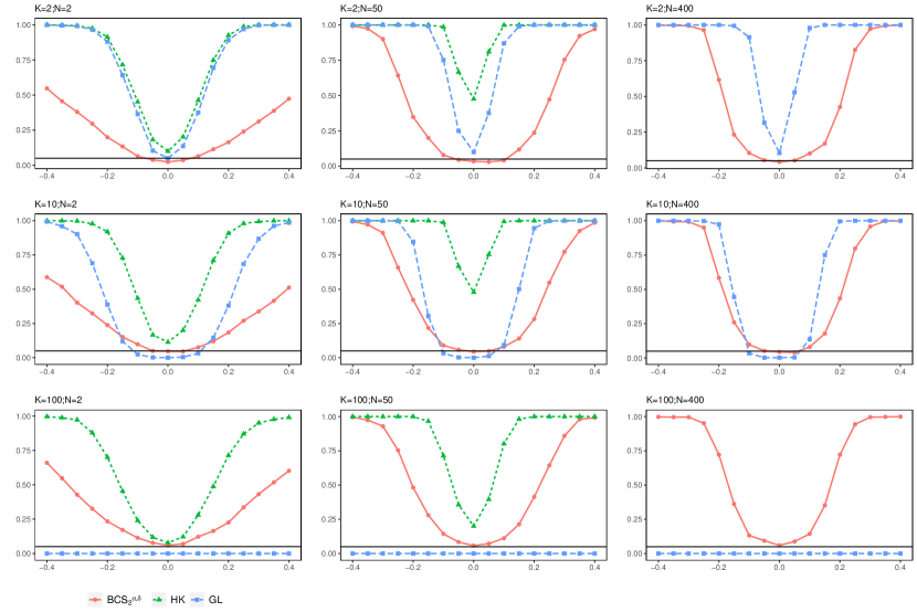
Figure 1: Empirical Power of the MVS Tests
The plots display the empirical power (over 500 replications) for the MVS tests $H_{0}^{\boldsymbol{\alpha},\boldsymbol{\delta}}$ under the AR-GARCH(1,1) model with skewed Student-$t$ errors for various $K$ benchmark and $N$ test assets. We consider $K\in\{2,10,100\}$ and $N\in\{2,50,400\}$. For $N=400$, the test HK is not feasible. The solid horizontal lines correspond to the nominal level of 5%.

3.4.2 Power Results for $H_{0}^{\boldsymbol{\alpha}}$

The power curves of the maximum Sharpe portfolio spanning tests $H_{0}^{\boldsymbol{\alpha}}$ are plotted in Figure 2. As for the joint test, the contribution of BCS${}^{\boldsymbol{\alpha}}_{2}$ is visible when the number of test assets is large. Indeed, unlike the GRS, F1, and BJ, this test is still applicable when $N>T$ and in this case, it has a decent size (unlike PY) and it has power against the null hypothesis $H_{0}^{\boldsymbol{\alpha}}$ (unlike GL).

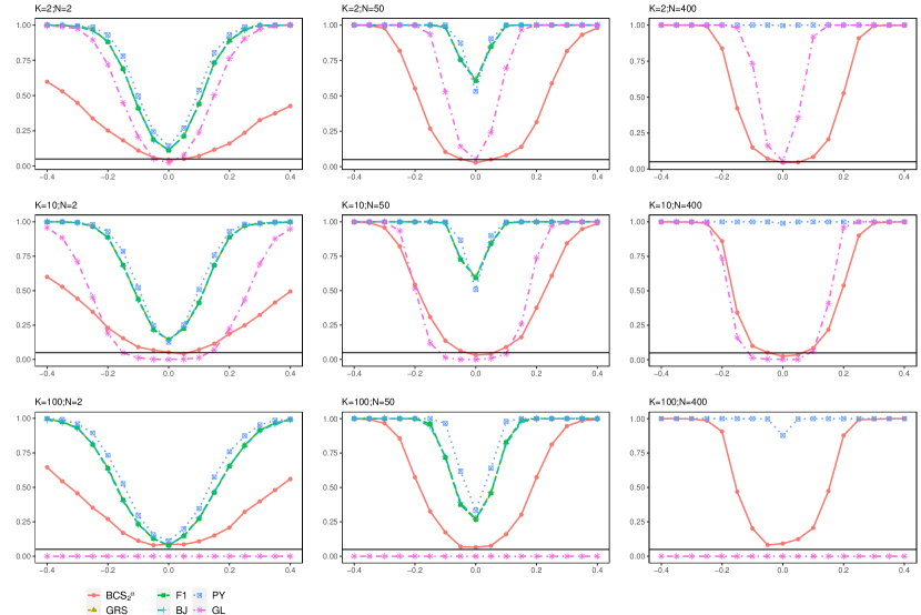
Figure 2: Empirical Power of the Maximum Sharpe Portfolio Spanning Tests
The plots display the empirical power (over 500 replications) of the maximum Sharpe portfolio spanning tests $H_{0}^{\boldsymbol{\alpha}}$ under the AR-GARCH(1,1) model with skewed Student-$t$ errors for $K$ benchmark and $N$ test assets. We consider $K\in\{2,10,100\}$ and $N\in\{2,50,400\}$. For $N=400$, the GRS, F1, and BJ tests are not feasible. The solid horizontal lines correspond to the nominal level of 5%.

3.4.3 Power Results for $H_{0}^{\boldsymbol{\delta}}$

Finally, the power curves of the minimum-variance portfolio spanning tests $H_{0}^{\boldsymbol{\delta}}$ are plotted in Figure 3. When $N=2$, KM and F2 have much higher power than BCS${}^{\boldsymbol{\delta}}_{2}$. When $N$ is moderately large (i.e., $N=50$), rejection frequencies of KM and F2 are higher than BCS${}^{\boldsymbol{\delta}}_{2}$ but these two tests are slightly oversized unlike BCS${}^{\boldsymbol{\delta}}_{2}$. When $N=400$, the only applicable test is BCS${}^{\boldsymbol{\delta}}_{2}$, and the power curves are again insensitive to the number of benchmark assets.

To sum up, the BCS${}^{\boldsymbol{\alpha},\boldsymbol{\delta}}_{2}$, BCS${}^{\boldsymbol{\alpha}}_{2}$ and BCS${}^{\boldsymbol{\delta}}_{2}$ tests are the ones retaining good properties in the presence of serial correlation and GARCH effects, even when the number of test and benchmark assets is large.

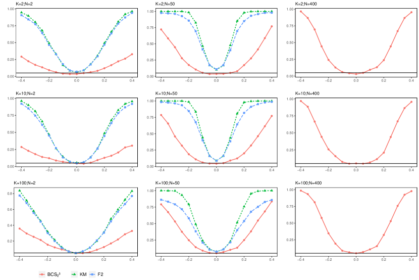
Figure 3: Empirical Power of the Global Minimum-Variance Portfolio Spanning Tests
The plots display the empirical power (over 500 replications) of the global minimum-variance portfolio spanning tests $H_{0}^{\boldsymbol{\delta}}$ under the AR-GARCH(1,1) model with skewed Student-$t$ errors for various $K$ benchmark and $N$ test assets. We consider $K\in\{2,10,100\}$ and $N\in\{2,50,400\}$. For $N=400$, the KM and F2 tests are not feasible. The solid horizontal lines correspond to the nominal level of 5%.

4 Empirical Application

This section tests to which extent domestic equity investors could benefit from international diversification. Our empirical illustration uses daily returns from 2007 to 2022 on blue-chip stocks traded in North America and Europe. Specifically, at the begining of each year, we use stock returns of the historical constituents in the following equity indices: (i) S&P 100 (U.S.), (ii) Euronext 100 (Eurozone), and (iii) SMI (Switzerland). We apply the three spanning tests $H_{0}^{\boldsymbol{\alpha},\boldsymbol{\delta}}$, $H_{0}^{\boldsymbol{\alpha}}$, and $H_{0}^{\boldsymbol{\delta}}$ every year to determine whether it is relevant to include assets from the other two countries. The number of benchmark and test assets varies slightly over time but remains a large-dimensional problem, and the sample size for each year is slightly less than 250 days; see the online appendix for details.

For BCS${}^{\boldsymbol{\lambda}}_{L}$, we set $L=2$ as the empirical size was found to be satisfactory in the Monte Carlo study for $T=250$. We consider a fixed-width rule $\zeta=1/3$, but results are robust to alternative choices. We compare our results for $H_{0}^{\boldsymbol{\alpha},\boldsymbol{\delta}}$ and $H_{0}^{\boldsymbol{\alpha}}$ with the GL approach using the default implementation with 500 boostrap replications. Results are reported in Table 5, where tests with a p-value lower that 5% are highlighted by a symbol $\checkmark$ while inconclusive test outcomes (of the GL tests) are highlighted by a question mark’.

First, we find that the test $H_{0}^{\boldsymbol{\alpha},\boldsymbol{\delta}}$ is rejected on average one-third of the time for each country and the rejections do not align among countries. Second, we see that the rejection of the MVS hypothesis comes from the potential of variance reduction in the domestic global minimum-variance portfolio. Rejections of $H_{0}^{\boldsymbol{\delta}}$ drives the rejection of $H_{0}^{\boldsymbol{\alpha},\boldsymbol{\delta}}$. On the contrary, the maximum Sharpe portfolio spanning test $H_{0}^{\boldsymbol{\alpha}}$ is only rejected a few times.

On the other hand, we are unable to consistently reject the null hypothesis $H_{0}^{\boldsymbol{\alpha},\boldsymbol{\delta}}$ using GL, leading to inconclusive results when $K$ is moderately large (see columns S&P 100 and Euronext 100). In slightly more than 25% of the cases, GL yields inconclusive results when test assets are SMI constituents. However, we do not reject $H_{0}^{\boldsymbol{\alpha},\boldsymbol{\delta}}$ using GL in 2007 and 2017 when test assets are S&P 100 constituents. We reject $H_{0}^{\boldsymbol{\alpha},\boldsymbol{\delta}}$ around 75% of the cases when SMI constituents are the test assets. This behavior of the GL test statistics is expected as it becomes less informative as $K$ increases (see Section 3.4.1). When focusing on $H_{0}^{\boldsymbol{\alpha}}$, we are unable to reject the null hypothesis of Sharpe ratio portfolio spanning with any of the test assets universes under consideration using GL. Overall, we can conclude that the few rejections of $H_{0}^{\boldsymbol{\alpha},\boldsymbol{\delta}}$ are driven by the rejection of $H_{0}^{\boldsymbol{\delta}}$. However, unlike BCS${}^{\boldsymbol{\lambda}}_{2}$, we obtain fewer rejections of $H_{0}^{\boldsymbol{\alpha},\boldsymbol{\delta}}$, which can be explained by the superior performance of BCS${}^{\boldsymbol{\lambda}}_{2}$ over GL in terms of size and power (see Sections 3.3 and 3.4).

Table 5: Results of the MVS Tests Over Time for the Various Investment Universes
This table reports the rejections at the 5% significance level (highlighted by a symbol $\checkmark$) of the various MVS tests applied at the asset level. $H_{0}^{\boldsymbol{\alpha},\boldsymbol{\delta}}$ is the MVS test, $H_{0}^{\boldsymbol{\alpha}}$ is the maximum Sharpe ratio spanning test, and $H_{0}^{\boldsymbol{\delta}}$ is the global minimum-variance spanning test. GL is the test by Gungor and Luger (2016) implemented with 500 bootstrap replications and BCS${}^{\boldsymbol{\lambda}}_{2}$ is the our BCS test with $L=2$. A question mark indicates an inconclusive test outcome.

	S&P 100					Euronext 100					SMI
	GL		BCS${}^{\boldsymbol{\lambda}}_{2}$			GL		BCS${}^{\boldsymbol{\lambda}}_{2}$			GL		BCS${}^{\boldsymbol{\lambda}}_{2}$
Year	$H_{0}^{\boldsymbol{\alpha},\boldsymbol{\delta}}$	$H_{0}^{\boldsymbol{\alpha}}$	$H_{0}^{\boldsymbol{\alpha},\boldsymbol{\delta}}$	$H_{0}^{\boldsymbol{\alpha}}$	$H_{0}^{\delta}$	$H_{0}^{\boldsymbol{\alpha},\boldsymbol{\delta}}$	$H_{0}^{\boldsymbol{\alpha}}$	$H_{0}^{\boldsymbol{\alpha},\boldsymbol{\delta}}$	$H_{0}^{\boldsymbol{\alpha}}$	$H_{0}^{\boldsymbol{\delta}}$	$H_{0}^{\boldsymbol{\alpha},\boldsymbol{\delta}}$	$H_{0}^{\boldsymbol{\alpha}}$	$H_{0}^{\boldsymbol{\alpha},\boldsymbol{\delta}}$	$H_{0}^{\boldsymbol{\alpha}}$	$H_{0}^{\boldsymbol{\delta}}$
2007						?				✓	✓		✓
2008	?		✓		✓	?		✓			?
2009	?		✓	✓	✓	?					?
2010	?		✓		✓	?					✓		✓		✓
2011	?					?		✓		✓	✓		✓		✓
2012	?					?					✓				✓
2013	?					?		✓			✓		✓		✓
2014	?				✓	?		✓		✓	✓			✓
2015	?		✓			?				✓	✓		✓		✓
2016	?				✓	?		✓		✓	✓		✓
2017					✓	?	?			✓	✓				✓
2018	?		✓		✓	?				✓	✓		✓		✓
2019	?		✓		✓	?		✓			✓				✓
2020	?		✓		✓	?					?
2021	?				✓	?			✓		✓		✓		✓
2022	?		✓		✓	?					?

5 Conclusion

The paper proposes a new framework for mean-variance spanning (MVS) testing that is more general and computationally efficient than existing methods. The proposed framework can be applied to any test-asset dimension and only requires stationary asset returns. It uses new moment conditions for spanning and tests them in two steps. First, it tests each component of the moment vector using robust Student-t tests based on the batch-mean method. Second, it combines the individual p-values using the Cauchy combination test (CCT) of Liu and Xie (2020), which accounts for the cross-sectional dependence between the test statistics. Monte Carlo simulations show the proposed MVS tests have correct sizes and high power in most setups. Unlike state-of-the-art methods, they also work well on skewed, heteroscedastic, and fat-tailed data. The methodology is applied to test if combining blue-chip stocks traded in the U.S., Europe, and Switzerland can improve each country’s domestic mean-variance efficient frontier. We find that the benefits of international diversification depend on economic conditions and vary across countries. We also highlight that the rejection of the MVS hypothesis originates from the potential to reduce variance within the domestic global minimum-variance portfolio.

Online Appendix
High-Dimensional Mean-Variance Spanning Tests

I Additional Lemma and Proofs

Lemma 1 derives the decomposition of a precision matrix using nodewize regressions. Similar results can also be found in Peng et al. (2009).

Lemma 1.

Consider the random vector $\mathbf{x}_{t}\in\mathbb{R}^{d}$ and the following sequence of $d$ regressions $x_{j,t}=\sum_{i=1,i\neq j}^{d}\theta_{i,j}x_{i,t}+v_{j,t}$ with $\mathbb{E}[\mathbf{x}_{-j,t}v_{j,t}]=0$ and $\mathbb{E}[v_{j,t}]=\mathbf{0}_{(d-1)\times 1}$ for $j=1,\ldots,d$. Let $\mathbb{V}[v_{i,t}]=g^{2}_{i}$ for $i=1,\ldots,d$, $\mathbf{G}\equiv\operatorname{Diag}(g^{2}_{1},\ldots,g^{2}_{d})$ and $\boldsymbol{\Theta}\equiv(\theta_{i,j})$.

1. Using the exogeneity conditions $\mathbb{E}[\mathbf{x}_{-j,t}v_{j,t}]=\mathbf{0}_{(d-1)\times 1}$ for any $j$, and $k\neq j$, one can deduce that $\mathbb{E}[v_{k},v_{j}]=\mathbb{E}[v_{k}(x_{j,t}-\sum_{i=1,i\neq j}^{d}\theta_{i,j}x_{i,t})]=-\theta_{j,k}\mathbb{E}[v_{k},x_{k}]=-\theta_{j,k}\mathbb{E}[v_{k},v_{k}]=-\theta_{j,k}\mathbb{V}(v_{k})=-\theta_{j,k}g_{k}$.

2. Therefore, $\boldsymbol{\Sigma}^{-1}=\mathbb{E}[\mathbf{x}_{t}\mathbf{x}_{t}^{\prime}]^{-1}=\mathbf{G}^{-1}(\mathbf{I}_{d}-\boldsymbol{\Theta})$ if $\mathbb{E}[\mathbf{x}_{t}\mathbf{x}_{t}^{\prime}]$ is invertible.

3. One also has that $\mathbb{E}[\mathbf{v}_{t}\mathbf{v}_{t}^{\prime}]=(\mathbf{I}_{d}-\boldsymbol{\Theta})\mathbf{G}$.

Lemma 1 suggests that Proposition 1 is valid for any $N$ and $K<T$.

Proof of Proposition 1.

The result follow from a direct application of Lemma 1 to $\mathbf{x}_{t}=(r_{1,t},1,r_{2,j,t}-r_{1,t},\mathbf{r}_{1,-1,t}^{\prime}-\mathbf{i}_{K-1}^{\prime}r_{1,t})^{\prime}$. See Section 2.2 in the paper for an illustration. ∎

Proof of Theorem 1.

Since for $b=1,\ldots,B$, $\hat{m}_{j}(\hat{\boldsymbol{\theta}}_{j})_{b}$ converges to $\hat{m}_{j}(\boldsymbol{\theta}_{j})_{b}$ at the rate $\sqrt{T}\gg\sqrt{T_{b}}$, standard results on batch-mean for mean estimate of a stationary sequence apply. That is, $\hat{v}_{j}(\hat{\boldsymbol{\theta}}_{j})_{\!B}-\mathbb{V}[m_{j}(\boldsymbol{\theta}_{j})]=o_{p}(1)$ while $m_{j}(\hat{\boldsymbol{\theta}}_{j})_{b}=m_{j}(\boldsymbol{\theta}_{j})_{b}+o_{p}(1)$ and $m_{j}(\hat{\boldsymbol{\theta}}_{j})_{b^{\prime}}=m_{j}(\boldsymbol{\theta}_{j})_{b^{\prime}}+o_{p}(1)$ have zero covariance whenever $b\neq b^{\prime}$ and $T\to\infty$. Furthermore, $\hat{m}_{j}(\hat{\boldsymbol{\theta}}_{j})_{1},\ldots,\hat{m}_{j}(\hat{\boldsymbol{\theta}}_{j})_{B-1}$ and $\hat{m}_{j}(\hat{\boldsymbol{\theta}})_{B}$ behave asymptotically as i.i.d. normal random variables with mean $m_{j}(\boldsymbol{\theta})$ and variance $\mathbb{V}[m_{j}(\boldsymbol{\theta}_{j})]$ (Carlstein et al., 1986). Therefore, we can apply a Student-t test to test the mean of the sample $\{m_{j}(\hat{\boldsymbol{\theta}}_{j})_{b}\}_{b=1}^{B}$ as in (13). We refer to Carlstein et al. (1986); Pedersen (2020) and subsequent references for more details about the theory of the batch-mean method for general statistics under mixing conditions. See also Zhang et al. (2017, Theorem 5.1 and 5.2.) for the rate of convergence of $(v_{1}(\hat{\boldsymbol{\theta}}_{j})_{\!B},\ldots,v_{d}(\hat{\boldsymbol{\theta}}_{j})_{\!B})^{\prime}$ under the physical dependence framework. ∎

II Additional Results

Table A.1 reports the sample size $T$, the number benchmark assets $K$, and the number of test assets $N$ used in the two empirical applications of Section 4 of the paper.

Table A.1: Dimensions of the Universes in the Empirical Applications
The table reports the number of observations $T$, the number of benchmark assets $K$, and test assets $N$ in the two empirical applications of Section 4. For the first application, the element under $N$ for a given benchmark universe equals the sum of those under the columns $K$ of the other benchmark assets, except for 2015. This is because of dual listed stocks in the SMI and Euronext 100. In the second application, the number of factors was the same every year: 5 for FF5, 6 for FF6, 25 for FF25, 100 for FF100, and 153 for KEW and KVW.

	Application 1							Application 2
		S&P 100		Euronext 100		SMI		S&P 500
Year	$T$	$K$	$N$	$K$	$N$	$K$	$N$	$T$	$N$
2007	244	99	118	98	119	20	197	251	496
2008	245	99	118	98	119	20	197	253	497
2009	245	100	115	96	119	19	196	252	498
2010	248	100	117	98	119	19	198	252	498
2011	248	100	115	95	120	20	195	252	496
2012	243	99	116	96	119	20	195	250	496
2013	243	100	119	99	120	20	199	252	497
2014	243	100	117	97	120	20	197	252	500
2015∗	246	101	118	99	120	20	199	252	495
2016	248	102	118	98	122	20	200	252	502
2017	245	101	119	99	121	20	200	251	502
2018	242	102	118	98	122	20	200	251	505
2019	243	100	116	97	119	19	197	252	500
2020	246	100	110	90	120	20	190	253	501
2021	248	101	103	83	121	20	184	252	504
2022	247	101	101	81	121	20	182	251	501

References

- Beaulieu et al. (2007) Beaulieu, M.C., Dufour, J.M., Khalaf, L., 2007. Multivariate tests of mean–variance efficiency with possibly non-gaussian errors: An exact simulation-based approach. Journal of Business & Economic Statistics 25, 398–410.
- Beaulieu et al. (2010) Beaulieu, M.C., Dufour, J.M., Khalaf, L., 2010. Asset-pricing anomalies and spanning: Multivariate and multifactor tests with heavy-tailed distributions. Journal of Empirical Finance 17, 763–782.
- Bekaert and Harvey (1995) Bekaert, G., Harvey, C.R., 1995. Time-varying world market integration. Journal of Finance 50, 403–444.
- Benjamini and Hochberg (1995) Benjamini, Y., Hochberg, Y., 1995. Controlling the false discovery rate: a practical and powerful approach to multiple testing. Journal of the Royal Statistical Society: Series B (Methodological) 57, 289–300.
- Benjamini and Yekutieli (2001) Benjamini, Y., Yekutieli, D., 2001. The control of the false discovery rate in multiple testing under dependency. Annals of Statistics , 1165–1188.
- Britten-Jones (1999) Britten-Jones, M., 1999. The sampling error in estimates of mean-variance efficient portfolio weights. Journal of Finance 54, 655–671.
- Carlstein (1986) Carlstein, E., 1986. Asymptotic normality for a general statistic from a stationary sequence. Annals of Probability 14.
- Carlstein et al. (1986) Carlstein, E., et al., 1986. The use of subseries values for estimating the variance of a general statistic from a stationary sequence. Annals of statistics 14, 1171–1179.
- Chen and Yuen (2009) Chen, Y., Yuen, K.C., 2009. Sums of pairwise quasi-asymptotically independent random variables with consistent variation. Stochastic Models 25, 76–89.
- Darolles et al. (2018) Darolles, S., Francq, C., Laurent, S., 2018. Asymptotics of cholesky garch models and time-varying conditional betas. Journal of Econometrics 204, 223–247.
- Demarta and McNeil (2005) Demarta, S., McNeil, A.J., 2005. The t copula and related copulas. International statistical review 73, 111–129.
- DeRoon and Nijman (2001) DeRoon, F.A., Nijman, T.E., 2001. Testing for mean-variance spanning: A survey. Journal of Empirical Finance 8, 111–155.
- Fama and French (1993) Fama, E.F., French, K.R., 1993. Common risk factors in the returns on stocks and bonds. Journal of Financial Economics 33, 3–56.
- Fernández and Steel (1998) Fernández, C., Steel, M.F.J., 1998. On bayesian modeling of fat tails and skewness. Journal of the American Statistical Association 93, 359–371.
- Flegal et al. (2010) Flegal, J.M., Jones, G.L., et al., 2010. Batch means and spectral variance estimators in Markov chain Monte Carlo. Annals of Statistics 38, 1034–1070.
- François and Hübner (2024) François, P., Hübner, G., 2024. The Complete Guide to Portfolio Performance. Appraise, Analyze, Act. Wiley. Under press.
- Gibbons et al. (1989) Gibbons, M.R., Ross, S.A., Shanken, J., 1989. A test of the efficiency of a given portfolio. Econometrica: Journal of the Econometric Society , 1121–1152.
- Giot and Laurent (2003) Giot, P., Laurent, S., 2003. Value-at-risk for long and short trading positions. Journal of Applied Econometrics 18, 641–663.
- Gungor and Luger (2009) Gungor, S., Luger, R., 2009. Exact distribution-free tests of mean-variance efficiency. Journal of Empirical Finance 16, 816–829.
- Gungor and Luger (2016) Gungor, S., Luger, R., 2016. Multivariate tests of mean-variance efficiency and spanning with a large number of assets and time-varying covariances. Journal of Business & Economic Statistics 34, 161–175.
- Hochberg (1988) Hochberg, Y., 1988. A sharper Bonferroni procedure for multiple tests of significance. Biometrika 75, 800–802.
- Holm (1979) Holm, S., 1979. A simple sequentially rejective multiple test procedure. Scandinavian Journal of Statistics , 65–70.
- Hommel (1988) Hommel, G., 1988. A stagewise rejective multiple test procedure based on a modified Bonferroni test. Biometrika 75, 383–386.
- Huberman and Kandel (1987) Huberman, G., Kandel, S., 1987. Mean-variance spanning. Journal of Finance 42, 873–888.
- Ibragimov and Müller (2010) Ibragimov, R., Müller, U.K., 2010. t-statistic based correlation and heterogeneity robust inference. Journal of Business & Economic Statistics 28, 453–468.
- Kan and Zhou (2012) Kan, R., Zhou, G., 2012. Tests of mean-variance spanning. Annals of Economics and Finance 13, 139–187.
- Kempf and Memmel (2006) Kempf, A., Memmel, C., 2006. Estimating the global minimum variance portfolio. Schmalenbach Business Review 58, 332–348.
- Lazarus et al. (2019) Lazarus, E., Lewis, D.J., Stock, J.H., 2019. The size-power tradeoff in har inference. Available at SSRN 3436372 .
- Lazarus et al. (2018) Lazarus, E., Lewis, D.J., Stock, J.H., Watson, M.W., 2018. Har inference: Recommendations for practice. Journal of Business & Economic Statistics 36, 541–559.
- Lee and Mykland (2008) Lee, S.S., Mykland, P.A., 2008. Jumps in financial markets: A new nonparametric test and jump dynamics. Review of Financial Studies 21, 2535–2563.
- Ling (2023) Ling, X., 2023. Additive P-Value Combination Test. Ph.D. thesis. Michigan Technological University.
- Lintner (1965) Lintner, J., 1965. The valuation of risk assets and the selection of risky investments in stock portfolios and capital budgets. Review of Economics and Statistics 47, 13–37.
- Liu and Xie (2020) Liu, Y., Xie, J., 2020. Cauchy combination test: A powerful test with analytic -value calculation under arbitrary dependency structures. Journal of the American Statistical Association 115, 393–402.
- Long et al. (2023) Long, M., Li, Z., Zhang, W., Li, Q., 2023. The Cauchy combination test under arbitrary dependence structures. The American Statistician 77, 134–142.
- Pedersen (2020) Pedersen, R.S., 2020. Robust inference in conditionally heteroskedastic autoregressions. Econometric Reviews 39, 244–259.
- Peng et al. (2009) Peng, J., Wang, P., Zhou, N., Zhu, J., 2009. Partial correlation estimation by joint sparse regression models. Journal of the American Statistical Association 104, 735–746.