A high-order explicit Runge-Kutta approximation technique for the Shallow Water Equations

Abstract

We introduce a high-order space-time approximation of the Shallow Water Equations with sources that is invariant-domain preserving (IDP) and well-balanced with respect to rest states. The employed time-stepping technique is a novel explicit Runge-Kutta (ERK) approach which is an extension of the class of ERK-IDP methods introduced by Ern and Guermond (SIAM J. Sci. Comput. 44(5), A3366–A3392, 2022) for systems of non-linear conservation equations. The resulting method is then numerically illustrated through verification and validation.

65M60, 65M12, 35L50, 35L65, 76M10

1 Introduction

The development of robust, accurate and efficient discretization techniques for the shallow water equations (and variations thereof) is an important task for the field of geosciences. These models are widely used for applications in coastal hydraulics, in-land flooding and climate prediction. Using numerical methods that are accurate in the temporal and spatial domain is desirable for such applications as long-time simulations spanning longer than 24 hours are common. Robustness is also an important criterion for such methods. Here, we say that a method is robust if it can handle dry states and if it can preserve important equilibrium states which could be either the rest state [5, 23] or time-independent solutions with nonzero velocity [41, 50, 13]. Numerical methods that preserve such equilibrium states are said to be well-balanced. The reader is referred to the book of Bouchut [8] for a review on issues related to well-balancing. Finally, to be useful for practitioners, numerical methods for solving the shallow water equations must be versatile; in particular, they must be able to handle unstructured meshes. But, achieving robustness with respect to dry states, well-balancing, and high-order accuracy in space and time on unstructured meshes is challenging. The task becomes even more complex when external source terms besides topography are added.

Developing well-balanced methods that are robust with respect to dry states is an active topic of research; see [3, 6, 20, 34, 42, 43]. Recent work on high-order schemes for the shallow water equations without external source terms that are well-balanced and robust with respect to dry states has been proposed in [11] for finite volumes + central WENO on structured meshes and in [31] for continuous finite elements on unstructured meshes. The reader is also referred to [37, 18, 13, 27] for other recent works that consider the inclusion of external source terms such as friction and rain effects. With the advancement of computing architectures, there has also been some development on efficient implementation of numerical methods for the shallow water equations; see e.g., [10, 17, 16, 12].

The goal of this work is to present an explicit approximation of the shallow water equations with topography and external sources that is well-balanced and high-order accurate in space and time. Our theoretical and algorithmic work is supplemented with a high performance implementation suitable for high fidelity simulations that is made freely available as part of the ryujin project [38, 30]. The purpose of this work is to provide a stepping stone for various multi-physics extensions of the shallow water equations that require an implicit-explicit (IMEX) time discretization. Such variations include the Serre-Green-Naghdi Equations [22, 46] for dispersive water waves and the coupling of the shallow water equations to subsurface models such as Richard’s equation. The starting point for this work are the approximation techniques introduced in [4, 27] for the shallow water equations. Unfortunately, the methodology discussed in [4, 27] has two drawbacks: (i) the high-order spatial approximation is not fully well-balanced when a shoreline is present; that is to say, the shoreline must coincide with the mesh for the method to maintain well-balancing. (ii) the time-discretization is limited in accuracy and efficiency due to the use of explicit strong stability preserving (SSP) explicit Runge-Kutta (ERK) methods which are known to be limited to fourth-order accuracy (see Ruuth and Spiteri [45, Thm. 4.1]) and generally have an efficiency ratio significantly smaller than one [19, Def. 1.1]. Here, we provide solutions to these drawbacks. Specifically, we revisit the low-order method proposed in [4, §3] and construct a high-oder version thereof that is unconditionally well-balanced and more robust with respect to dry states than the ones outlined in [4, §4] and [27, §5&6]. The novelty of the spatial discretization introduced in this work is threefold: (i) we introduce modified auxiliary states (see Eq. (3.5)) that act as local Riemann averages for hydrostatic reconstructed left/right states; (ii) we rewrite the low-order method as a convex combination of these auxiliary states and external source terms (see Lemma 3.6); (iii) we introduce novel local bounds in space and time that control the updated velocity thereby avoiding blow-up and unnecessary time-step restrictions (see Lemma 3.12). These modifications allow the final limited updated to be high-order accurate in space and time, invariant-domain preserving and well-balanced w.r.t. rest states without any restrictions on the underlying mesh.

The paper is organized as follows. We briefly present the mathematical model and relevant properties in Section 2. In Section 3, we introduce a discretization-independent high-order spatial approximation to the shallow water equations with forward Euler time stepping and a convex limiting procedure. The main results of this section are Lemma 3.6, Proposition 3.9, Proposition 3.18 and Proposition 3.20. Then, using the convex limiting methodology used for high-order spatial discretization, we introduce in Section 4 a high-order in time invariant-domain preserving (IDP) explicit Runge-Kutta (ERK) method. Finally, we verify and validate the numerical method in Section 5. For the sake of completeness, we detail the implementation of boundary conditions for our method in Appendix A.

2 The model problem

Let $D$ be a polygonal domain in ${\mathbb{R}}^{d}$, $d\in\{1,2\}$, occupied by a body of water whose evolution in time under the action of gravity is modeled by the shallow water equations (also known as the Saint-Venant equations). Let ${\bm{x}}\in D$ be the position vector and $t>0$ be the time variable. Let ${\bm{u}}:=(\mathsf{h},{\bm{q}})^{\mathsf{T}}\in{\mathbb{R}}^{d+1}$ be the dependent variable of the system where $\mathsf{h}({\bm{x}},t)$ is the water depth and ${\bm{q}}({\bm{x}},t)\in{\mathbb{R}}^{d}$ is the depth-averaged momentum vector of the fluid, also called discharge. Let $z({\bm{x}})$ be the known topography mapping. We henceforth assume that $z$ is in $W^{1,\infty}(D;{\mathbb{R}})$ to make sure that $\nabla z$ is a bounded function and thereby avoiding the need of properly defining $\mathsf{h}\nabla z$ when $z$ is discontinuous. The goal of this work is to solve the following system of partial differential equations in the weak sense:

(2.1a) $$\begin{aligned} &\partial_{t}{\bm{u}}+\nabla{\cdot}{\mathbbm{f}}({\bm{u}})={\mathbbm{b}}({\bm{u}},z({\bm{x}}))&&\text{for a.e.\@\ }t>0,\,{\bm{x}}\in D,\\ &{\bm{u}}({\bm{x}},0)={\bm{u}}_{0}({\bm{x}})&&\text{for a.e.\@\ }{\bm{x}}\in D,\end{aligned}$$

with ${\mathbbm{f}}({\bm{u}}):=({\bm{q}},{\bm{q}}\otimes{\bm{v}}+\frac{1}{2}g\mathsf{h}^{2}{\mathbb{I}}_{d})^{\mathsf{T}}$ and ${\mathbbm{b}}({\bm{u}},z({\bm{x}})):=(0,-g\mathsf{h}\nabla z)^{\mathsf{T}}$ where ${\bm{v}}:=\mathsf{h}^{-1}{\bm{q}}\in{\mathbb{R}}^{d}$ is the (depth-averaged) velocity vector, $g$ is the gravitational acceleration constant, and ${\mathbb{I}}_{d}\in{\mathbb{R}}^{d\times d}$ is the identity matrix. For the sake of completeness, we state a few properties regarding (2.1) that will be useful when constructing physically relevant approximations at the discrete level.

Definition 2.1 (Invariant set).

The following convex domain is an invariant set (in the sense of [25, Def. 2.3]) for the shallow water equations (2.1):

(2.2) $${\mathcal{A}}:=\big{\{}{\bm{u}}=(\mathsf{h},{\bm{q}})^{\mathsf{T}}\in{\mathbb{R}}^{d+1}\mid\mathsf{h}>0\big{\}}.$$

$\square$

When the fluid is at rest, i.e., ${\bm{q}}\equiv\bm{0}$, the Shallow Water Equations (2.1) reduce to $g\mathsf{h}\nabla(\mathsf{h}+z)=\bm{0}$, which motivates to introduce the following terminology.

Definition 2.2 (Problem at rest).

A solution ${\bm{u}}({\bm{x}},t)$ to the shallow water equations is said to be at rest at time $t$ if

$$\begin{aligned} {\bm{q}}(x,t)&=\bm{0}&\;&\text{for a.e.\@\ }{\bm{x}}\in D,\quad\text{and}\\ (\mathsf{h}+z)({\bm{x}},t)&=\text{const.}&\;&\text{a.e.\@\ on connected components of }\big{\{}{\bm{x}}\in D\;:\;\mathsf{h}({\bm{x}},t)>0\big{\}}.\end{aligned}$$

$\square$

Definition 2.3 (Entropy pairs and entropy solutions).

The pair $\big{(}E({\bm{u}}),{\bm{F}}({\bm{u}})\big{)}$:

(2.3) $$E({\bm{u}}):=\tfrac{1}{2}g\mathsf{h}^{2}+\tfrac{1}{2}\mathsf{h}\|{\bm{v}}\|^{2}+gz\mathsf{h}, {\bm{F}}({\bm{u}}):={\bm{v}}\big{(}E({\bm{u}})+\tfrac{1}{2}g\mathsf{h}^{2}\big{)},$$

is an entropy pair for the shallow water equations (2.1) i.e., it satisfies $\nabla{\cdot}{\bm{F}}({\bm{u}})=\big{(}\nabla_{\bm{u}}E({\bm{u}})\big{)}^{\mathsf{T}}(\nabla{\cdot}{\mathbbm{f}}({\bm{u}})-{\mathbbm{b}}({\bm{u}},z({\bm{x}})))$. We call ${\bm{u}}({\bm{x}},t)$ an entropy solution to (2.1) if it is a weak solution to (2.1) and additionally satisfies the following inequality in the weak sense: $\partial_{t}E({\bm{u}})+\nabla{\cdot}{\bm{F}}({\bm{u}})\leq 0$. $\square$

Remark 2.4 (Entropy pair for flat topography).

When there is no influence due to topography ($z({\bm{x}})\equiv 0$), the entropy pair (2.3) simplifies to:

(2.4) $$E_{\text{flat}}({\bm{u}}):=\tfrac{1}{2}g\mathsf{h}^{2}+\tfrac{1}{2}\mathsf{h}\|{\bm{v}}\|^{2}, {\bm{F}}_{\text{flat}}({\bm{u}}):={\bm{v}}\big{(}E_{\text{flat}}({\bm{u}})+\tfrac{1}{2}g\mathsf{h}^{2}\big{)}.$$

and satisfies $\nabla{\cdot}{\bm{F}}_{\text{flat}}({\bm{u}})=\big{(}\nabla_{\bm{u}}E_{\text{flat}}({\bm{u}})\big{)}^{\mathsf{T}}\nabla{\cdot}{\mathbbm{f}}({\bm{u}})$. $\square$

For various applications, the system (2.1) is augmented with external source terms. Some examples include forcing due to bottom friction and source/sink of the water depth [13], Coriolis force [14] and many others. In this work, we only consider a simple time-independent source due to rainfall and and the loss of discharge due to the Gauckler-Manning friction force:

(2.5) $$\bm{S}({\bm{u}})=(R({\bm{x}}),-gn^{2}\mathsf{h}^{-\tfrac{4}{3}}{\bm{q}}\|{\bm{v}}\|_{\ell^{2}})^{\mathsf{T}},$$

where $R({\bm{x}})>0$ and $n$ is the Gauckler-Manning roughness coefficient.

3 Well-balanced forward Euler method

In this section, we introduce a forward Euler approximation to the shallow water equations that is high-order accurate in space, well-balanced and invariant-domain preserving. This section lays the foundation for the high-order explicit Runge-Kutta methodology introduced in Section 4.

3.1 Approximation details

Let $(0,T)$ be a chosen time interval for (2.1). Let$\{t^{n}\}_{n\in\{0\hskip 0.35002pt{:}\hskip 0.70004ptN\}}$ be a discretization of $(0,T)$ with the convention that $N\geq 1$, $t^{0}=0$, and $t^{N}=T$. The spatial approximation is discretization independent and can be either finite differences, finite volumes, continuous or discontinuous finite elements. Letting $t^{n}$ be the current discrete time, we assume that the spatial approximation of ${\bm{u}}(\cdot,t^{n})$ is entirely defined by the collection of states $\textsf{{U}}^{n}:=\{\textsf{{U}}_{i}^{n}\}_{i\in{\mathcal{V}}}$, where ${\mathcal{V}}=\{1\hskip 0.50003pt{:}\hskip 1.00006ptI\}$ is the index set for the spatial degrees of freedom and $\textsf{{U}}_{i}^{n}:=({\mathsf{H}}_{i}^{n},\textsf{{Q}}_{i}^{n})^{\mathsf{T}}\in{\mathbb{R}}^{d+1}$. Here, ${\mathsf{H}}_{i}^{n}$ and $\textsf{{Q}}_{i}^{n}$ represent approximations of the water depth and discharge associated with the $i$-th degree of freedom at time $t^{n}$. To be able to refer to the water depth and the discharge of an arbitrary state $\tilde{\textsf{{U}}}=(\tilde{\mathsf{H}},\tilde{\textsf{{Q}}})$ in ${\mathbb{R}}^{d+1}$, we introduce the linear mappings ${\mathsf{H}}:{\mathbb{R}}^{d+1}\to{\mathbb{R}}$ and $\textsf{{Q}}:{\mathbb{R}}^{d+1}\to{\mathbb{R}}^{d}$ so that ${\mathsf{H}}(\tilde{\textsf{{U}}})=\tilde{\mathsf{H}}$ and $\textsf{{Q}}(\tilde{\textsf{{U}}})=\tilde{\textsf{{Q}}}$. We assume that the topography mapping is approximated by the collection of states: ${\mathsf{Z}}:=\{{\mathsf{Z}}_{i}\}_{i\in{\mathcal{V}}}$. We assume that for every $i\in{\mathcal{V}}$, there exists a subset ${\mathcal{I}}(i)\subsetneq{\mathcal{V}}$ that collects the local degrees of freedom that interact with $i$, which we call stencil at $i$. Let ${\mathcal{I}}^{*}(i):={\mathcal{I}}(i){\setminus}\{i\}$. We assume that the underlying spatial discretization provides the following three quantities for all $i\in{\mathcal{V}}$ and all $j\in{\mathcal{I}}(i)$:

1. An invertible low-order mass matrix ${\mathbb{M}}_{ij}^{\textup{L}}=m_{i}\delta_{ij}$ where $m_{i}>0$ is called the mass associated with the $i$-th degree of freedom;

2. An invertible, symmetric high-order matrix with entries ${\mathbb{M}}_{ij}^{\textup{H}}=m_{ij}$ such that: $({\mathbb{M}}^{\textup{H}}{\mathsf{X}})_{i}=\sum_{j\in{\mathcal{I}}(i)}m_{ij}{\mathsf{X}}_{j}$ for all ${\mathsf{X}}\in{\mathbb{R}}^{I}$;

3. A vector ${\bm{c}}_{ij}\in{\mathbb{R}}^{d}$ that approximates the gradient operator: $\nabla{\mathsf{X}}(t^{n})\approx\sum_{j\in{\mathcal{I}}(i)}{\mathsf{X}}_{j}^{n}{\bm{c}}_{ij}$.

The local stencil ${\mathcal{I}}(i)$ is more precisely defined by $(j\notin{\mathcal{I}}(i))\implies({\bm{c}}_{ij}=\bm{0}$ and $m_{ij}=0$). We further assume that ${\bm{c}}_{ij}=-{\bm{c}}_{ji}$ whenever $i$ or $j$ is not a boundary degree of freedom, and $\sum_{j\in{\mathcal{I}}(i)}{\bm{c}}_{ij}=0$ which is necessary for mass conservation. The high-order mass matrix is related to the low-order mass matrix through the relation $m_{i}=\sum_{j\in{\mathcal{I}}(i)}m_{ij}$ to guarantee that ${\mathbb{M}}^{\textup{L}}$ and ${\mathbb{M}}^{\textup{H}}$ carry the same mass: $\sum_{i\in{\mathcal{V}}}m_{i}\textsf{{U}}_{i}^{n}=\sum_{i\in{\mathcal{V}}}\sum_{j\in{\mathcal{I}}(i)}m_{ij}\textsf{{U}}_{j}^{n}$. Examples of discretization techniques satisfying the above assumptions are described in [28].

3.2 Well-balancing preliminaries

Before introducing the low- and high-order spatial approximations, we first define the discrete velocity and what it means to be well-balanced with respect to rest states. Given a state $({\mathsf{H}}_{i}^{n},\textsf{{Q}}_{i}^{n})^{\mathsf{T}}$ with nonzero water depth, ${\mathsf{H}}_{i}^{n}>0$, the velocity is defined to be the ratio $\textsf{{Q}}_{i}^{n}/{\mathsf{H}}_{i}^{n}$. To be robust with respect to dry states, we adopt the regularization technique from Kurganov and Petrova [34] that avoids the division by zero when ${\mathsf{H}}_{i}^{n}\rightarrow 0$. For this purpose, we introduce a small dimensionless parameter $\epsilon$ and a characteristic length scale $\mathsf{h}_{\max}$ that scales like the average of the water depth in the problem, and we set

(3.1) $$\textsf{{V}}_{i}^{n}:=\frac{2{\mathsf{H}}_{i}^{n}}{({\mathsf{H}}_{i}^{n})^{2}+\max({\mathsf{H}}_{i}^{n},\epsilon\mathsf{h}_{\max})^{2}}\textsf{{Q}}_{i}^{n}.$$

Notice that $\textsf{{V}}_{i}^{n}=\textsf{{Q}}_{i}^{n}/{\mathsf{H}}_{i}^{n}$ when ${\mathsf{H}}_{i}^{n}\geq\epsilon\mathsf{h}_{\max}$; that is, the regularization is active only when ${\mathsf{H}}_{i}^{n}\leq\epsilon\mathsf{h}_{\max}$. All the numerical simulations reported in the paper are done with $\epsilon=10^{-12}$ and using double precision floating point arithmetic. The well-balancing techniques in this work adopt the methodology proposed in Audusse et al. [3], Audusse and Bristeau [2] known as hydrostatic reconstruction of the water depth.

Definition 3.1 (Hydrostatic reconstruction).

For $i\in{\mathcal{V}}$ and $j\in{\mathcal{I}}(i)$, the hydrostatic reconstruction between $i$ and $j$ of the state $\textsf{{U}}_{i}$ and the associated water depth ${\mathsf{H}}_{i}$ are defined as follows:

(3.2a) $${\mathsf{H}}_{i}^{j,*} :=\max(0,{\mathsf{H}}_{i}+{\mathsf{Z}}_{i}-\max({\mathsf{Z}}_{i},{\mathsf{Z}}_{j})),$$

(3.2b) $$\textsf{{U}}_{i}^{j,*} :=\begin{pmatrix}{\mathsf{H}}_{i}^{*,j}\\ \textsf{{V}}_{i}{\mathsf{H}}_{i}^{j,*}\end{pmatrix}.$$

$\square$

Definition 3.2 (Discrete states at rest).

A given set of discrete numerical states $\{({\mathsf{H}}_{i}^{n},\textsf{{Q}}_{i}^{n})\}_{i\in{\mathcal{V}}}$ is said to be at rest if the approximate momentum $\textsf{{Q}}_{i}^{n}$ is zero for all $i\in{\mathcal{V}}$, and if the approximate water depth ${\mathsf{H}}_{i}^{n}$ and the approximate bathymetry map ${\mathsf{Z}}_{i}$ satisfy the following property for all $i\in{\mathcal{V}}$: ${\mathsf{H}}_{i}^{n,j,*}={\mathsf{H}}_{j}^{n,i,*}$ for all $j\in{\mathcal{I}}(i)$. $\square$

Remark 3.3.

Note that we have adopted the condition ${\mathsf{H}}_{i}^{n,j,*}={\mathsf{H}}_{j}^{n,i,*}$ to be the discrete analog to $(\mathsf{h}+z)({\bm{x}},t)=const.$ in Def. 2.2 instead of the natural looking identity ${\mathsf{H}}_{i}^{n}+{\mathsf{Z}}_{i}={\mathsf{H}}_{j}+{\mathsf{Z}}_{j}$. The reason behind this choice is the fact that Def. 3.2 does not need to distinguish between dry and wet states. For example, assume that ${\mathsf{H}}_{j}=0$ and ${\mathsf{Z}}_{i}>{\mathsf{Z}}_{j}$ for all $j\in{\mathcal{I}}(i)$. Then, ${\mathsf{H}}_{i}^{n,j,*}=\max(0,0+{\mathsf{Z}}_{i}-{\mathsf{Z}}_{i})=0$ and ${\mathsf{H}}_{j}^{n,i,*}=\max(0,0+{\mathsf{Z}}_{j}-{\mathsf{Z}}_{i})=0$, which gives ${\mathsf{H}}_{i}^{n,j,*}={\mathsf{H}}_{j}^{n,i,*}$. However, the condition ${\mathsf{H}}_{i}^{n}+{\mathsf{Z}}_{i}={\mathsf{H}}_{j}+{\mathsf{Z}}_{j}$ breaks down in this case since ${\mathsf{H}}_{j}=0$ for all $j\in{\mathcal{I}}(i)$ would imply that the topography mapping should be constant which is not the case. $\square$

3.3 Low-order spatial approximation

We now discuss a low-order method that will serve as safeguard to the high-order method. We essentially follow Azerad et al. [4, Sec. 3] which introduced a formally first-order consistent approximation of the shallow water equations when the spatial discretization consists of continuous, linear finite elements. But departing from Azerad et al. [4] we introduce a different definition of the auxiliary states (see Eq. 3.5) and introduce a different convex combination of theses auxiliary states to reconstruct the low order update; see Lemma 3.6.

Let $t^{n}$ be the current time and let ${\tau}:=t^{n+1}-t^{n}$ denote the current time step. The low-order approximation with forward Euler time-stepping is then given by:

(3.3a) $$\frac{m_{i}}{\tau}(\textsf{{U}}_{i}^{\textup{L},n+1}-\textsf{{U}}_{i}^{n})=\sum_{j\in{\mathcal{I}}(i)}\textsf{{F}}^{\textup{L},n}_{ij},$$

(3.3b) $$\begin{aligned} \textsf{{F}}^{\textup{L},n}_{ij}:={}&-\left(\!\textsf{{U}}_{j}^{n,i,*}\otimes\textsf{{V}}_{j}^{n}+\textsf{{U}}_{i}^{n,j,*}\otimes\textsf{{V}}_{i}^{n}\!\right){\bm{c}}_{ij}+d_{ij}^{\textup{L},n}\!\left(\!\textsf{{U}}_{j}^{n,i,*}-\textsf{{U}}_{i}^{n,j,*}\!\right)\\ &-\begin{pmatrix}0\\ g{\bm{c}}_{ij}\left(\frac{1}{2}({\mathsf{H}}_{j}^{n,i,*})^{2}-\frac{1}{2}({\mathsf{H}}_{i}^{n,j,*})^{2}+({\mathsf{H}}_{i}^{n})^{2}\right)\end{pmatrix}.\end{aligned}$$

Here, $d_{ij}^{\textup{L},n}\geq 0$ is the graph-viscosity coefficient that makes the method invariant-domain-preserving:

(3.4) $$d_{ij}^{\textup{L},n}:=\max\Big{(}\lambda_{\max}(\textsf{{U}}_{i}^{n,j,*},\textsf{{U}}_{j}^{n,i,*},{\bm{n}}_{ij})\|{\bm{c}}_{ij}\|_{\ell^{2}},\lambda_{\max}(\textsf{{U}}_{j}^{n,i,*},\textsf{{U}}_{i}^{n,j,*},{\bm{n}}_{ji})\|{\bm{c}}_{ji}\|_{\ell^{2}},\Big{)},$$

where ${\bm{n}}_{ij}:={\bm{c}}_{ij}/\|{\bm{c}}_{ij}\|_{\ell^{2}}$ and $\lambda_{\max}(\textsf{{U}}_{i}^{n,j,*},\textsf{{U}}_{j}^{n,i,*},{\bm{n}}_{ij})$ is a guaranteed upper bound on the maximum wave speed in the local Riemann problem with left and right states $(\textsf{{U}}_{i}^{n,j,*},\textsf{{U}}_{j}^{n,i,*})$ and flux ${\mathbbm{f}}(\cdot){\bm{n}}_{ij}$. Analytical expressions for $\lambda_{\max}$ are given in [4, Lem. 3.8]. Note that $d_{ij}^{\textup{L},n}=d_{ji}^{\textup{L},n}$ which is necessary for mass conservation. By convention, we set $d_{ii}^{\textup{L},n}:=-\sum_{j\in{\mathcal{I}}^{*}(i)}d_{ij}^{\textup{L},n}$. Observe that $\textsf{{F}}_{ij}^{\textup{L},n}=-\textsf{{F}}_{ji}^{\textup{L},n}$ when the topography is flat.

Lemma 3.4 (Well-balancing and conservation).

The scheme $\textsf{{U}}^{n}\mapsto\textsf{{U}}^{\textup{L},n+1}$ defined in (3.3) is mass-conservative and well-balanced. $\square$

Proof 3.5.

See Azerad et al. [4, Prop. 3.9]. $\square$

We now introduce auxiliary states that are meant to be thought of as averages of the self-similar solution to the local Riemann problem for the pair $(\textsf{{U}}_{i}^{n,j,*},\textsf{{U}}_{j}^{n,i,*})$ in the direction ${\bm{n}}_{ij}$. We do this to rewrite the low-order scheme (3.3) as a convex combination of these auxiliary states and source terms to extract local bounds in space and time. These bounds are needed for the convex limiting procedure described in Section 3.5. The importance of such auxiliary states for nonlinear conservation laws has been established in the literature and we refer the reader to Harten et al. [32], Nessyahu and Tadmor [40] and the references therein.

Let $i\in{\mathcal{V}}$. For every $j\in{\mathcal{I}}(i)$, we define the following auxiliary states for the pair $(i,j)$ as follows:

(3.5) $$\overline{\textsf{{U}}}_{ij}^{n}:=\frac{1}{2}\big{\{}\textsf{{U}}_{i}^{n,j,*}+\textsf{{U}}_{j}^{n,i,*}\big{\}}-\frac{1}{2d_{ij}^{\textup{L},n}}\big{\{}{\mathbbm{f}}(\textsf{{U}}_{j}^{n,i,*})-{\mathbbm{f}}(\textsf{{U}}_{i}^{n,j,*})\big{\}}{\bm{c}}_{ij},$$

with the convention that $\overline{\textsf{{U}}}_{ii}^{n}:=\textsf{{U}}_{i}^{n}$. We recall that $\overline{\textsf{{U}}}_{ij}^{n}$ coincides with the exact space average over $[-\frac{1}{2},\frac{1}{2}]$ at time $\frac{\|{\bm{c}}_{ij}\|_{\ell^{2}}}{2d_{ij}^{\textup{L},n}}$ of the solution to the Riemann problem with left and right states $(\textsf{{U}}_{i}^{n,j,*},\textsf{{U}}_{j}^{n,i,*})$ and with flux ${\mathbbm{f}}(v){\bm{n}}_{ij}$ provided the viscosity $d_{ij}^{\textup{L},n}$ is large enough so that $\lambda_{\max}(\textsf{{U}}_{i}^{n,j,*},\textsf{{U}}_{j}^{n,i,*},{\bm{n}}_{ij})\|{\bm{c}}_{ij}\|_{\ell^{2}},\leq d_{ij}^{\textup{L},n}$. Note that the bar states here differ from those in [4, Prop. 3.11]. We also define an affine shift needed for the convex combination update:

(3.6) $$\textsf{{B}}^{\textup{L},n}_{i}:=\sum_{j\in{\mathcal{I}}(i)}\textsf{{B}}^{\textup{L},n}_{ij},\quad\textsf{{B}}^{\textup{L},n}_{ij}:=-2(d_{ij}^{\textup{L},n}+\textsf{{V}}_{i}^{n}{\cdot}{\bm{c}}_{ij})(\textsf{{U}}_{i}^{n,j,*}-\textsf{{U}}_{i}^{n}).$$

Lemma 3.6 (Stability).

Assume that $\textsf{{U}}_{i}^{n}\in{\mathcal{A}}$ for all $i\in{\mathcal{V}}$. Assume also that the time step satisfies the restriction ${\tau}\leq\min_{i\in{\mathcal{V}}}\frac{m_{i}}{2|d_{ii}^{\textup{L},n}|}$. Then,

1. The following convex combination holds:

   (3.7) $$\textsf{{U}}_{i}^{\textup{L},n+1}=\Big{(}1+\frac{2\tau d_{ii}^{\textup{L},n}}{m_{i}}\Big{)}(\textsf{{U}}_{i}^{n}+\frac{\tau}{m_{i}}\textsf{{B}}^{\textup{L},n}_{i})+\sum_{j\in{\mathcal{I}}^{*}(i)}\frac{2\tau d_{ij}^{\textup{L},n}}{m_{i}}(\overline{\textsf{{U}}}_{ij}^{n}+\frac{\tau}{m_{i}}\textsf{{B}}^{\textup{L},n}_{i}).$$

2. The water depth of $\textsf{{U}}^{\textup{L},n+1}$ is positive, i.e., $\textsf{{U}}_{i}^{\textup{L},n+1}\in{\mathcal{A}}$ for all $i\in{\mathcal{V}}$.

$\square$

Proof 3.7.

In order to show (i) we add and subtract $\textsf{{B}}^{\textup{L},n}_{i}$ in (3.3) and then rearrange:

$$\frac{m_{i}}{\tau}(\textsf{{U}}_{i}^{\textup{L},n+1}-\textsf{{U}}_{i}^{n}) =\textsf{{B}}^{\textup{L},n}_{i}+\sum_{j\in{\mathcal{I}}(i)}\left[\textsf{{F}}^{\textup{L},n}_{ij}-\textsf{{B}}^{\textup{L},n}_{ij}\right].$$

Recalling that ${\mathbbm{f}}({\bm{u}}):=({\bm{q}},{\bm{q}}\otimes{\bm{v}}+\frac{1}{2}g\mathsf{h}^{2}{\mathbb{I}}_{d})^{\mathsf{T}}$ and $\sum_{j\in{\mathcal{I}}(i)}{\bm{c}}_{ij}=\bm{0}$, we have

$$\sum_{j\in{\mathcal{I}}(i)}\textsf{{F}}^{\textup{L},n}_{ij}-\textsf{{B}}^{\textup{L},n}_{ij} =\sum_{j\in{\mathcal{I}}(i)}-\{{\mathbbm{f}}(\textsf{{U}}_{j}^{n,i,*})-{\mathbbm{f}}(\textsf{{U}}_{i}^{n,j,*})\}{\bm{c}}_{ij}+d_{ij}^{\textup{L},n}\{\textsf{{U}}_{i}^{n,j,*}+\textsf{{U}}_{j}^{n,i,*}\},$$

$$=\sum_{j\in{\mathcal{I}}(i)}2d_{ij}^{\textup{L},n}\overline{\textsf{{U}}}_{ij}^{n}.$$

Then, recalling that $\overline{\textsf{{U}}}_{ii}^{n}=\textsf{{U}}_{i}^{n}$, and $\sum_{j\in{\mathcal{I}}(i)}d_{ij}^{\textup{L},n}=0$ holds true by virtue of the definition of $d_{ii}^{\textup{L},n}$, we infer that

$$\textsf{{U}}_{i}^{\textup{L},n+1} =\textsf{{U}}_{i}^{n}+\frac{\tau}{m_{i}}\textsf{{B}}^{\textup{L},n}_{i}+\sum_{j\in{\mathcal{I}}(i)}\frac{2\tau d_{ij}^{\textup{L},n}}{m_{i}}\overline{\textsf{{U}}}_{ij}^{n},$$

$$=\textsf{{U}}_{i}^{n}+\frac{\tau}{m_{i}}\textsf{{B}}^{\textup{L},n}_{i}+\frac{2\tau d_{ii}^{\textup{L},n}}{m_{i}}\textsf{{U}}_{i}^{n}+\sum_{j\in{\mathcal{I}}^{*}(i)}\frac{2\tau d_{ij}^{\textup{L},n}}{m_{i}}\overline{\textsf{{U}}}_{ij}^{n},$$

$$=\textsf{{U}}_{i}^{n}+\frac{\tau}{m_{i}}\textsf{{B}}^{\textup{L},n}_{i}+\frac{2\tau d_{ii}^{\textup{L},n}}{m_{i}}(\textsf{{U}}_{i}^{n}+\frac{\tau}{m_{i}}\textsf{{B}}^{\textup{L},n}_{i})+\sum_{j\in{\mathcal{I}}^{*}(i)}\frac{2\tau d_{ij}^{\textup{L},n}}{m_{i}}(\overline{\textsf{{U}}}_{ij}^{n}+\frac{\tau}{m_{i}}\textsf{{B}}^{\textup{L},n}_{i}),$$

$$=\Big{(}1+\frac{2\tau d_{ii}^{\textup{L},n}}{m_{i}}\Big{)}(\textsf{{U}}_{i}^{n}+\frac{\tau}{m_{i}}\textsf{{B}}^{\textup{L},n}_{i})+\sum_{j\in{\mathcal{I}}^{*}(i)}\frac{2\tau d_{ij}^{\textup{L},n}}{m_{i}}(\overline{\textsf{{U}}}_{ij}^{n}+\frac{\tau}{m_{i}}\textsf{{B}}^{\textup{L},n}_{i}).$$

The above decomposition is a genuine convex combination under the CFL condition $1+\frac{2\tau|d_{ii}^{\textup{L},n}|}{m_{i}}\geq 0$.

For (ii) we recall that the water depth of the sate $\textsf{{B}}_{i}^{\textup{L},n}$ is given by

$${\mathsf{H}}(\textsf{{B}}_{i}^{\textup{L},n}):=\sum_{j\in{\mathcal{I}}(i)}2(d_{ij}^{\textup{L},n}+\textsf{{V}}_{i}^{n}{\cdot}{\bm{c}}_{ij})({\mathsf{H}}_{i}^{n}-{\mathsf{H}}_{i}^{n,j,*}).$$

It is established in [4, Prop. 3.7] that $d_{ij}^{\textup{L},n}+\textsf{{V}}_{i}^{n}{\cdot}{\bm{c}}_{ij}\geq 0$ and by definition we have $({\mathsf{H}}_{i}^{n}-{\mathsf{H}}_{i}^{n,j,*})\geq 0$. Hence, ${\mathsf{H}}(\textsf{{B}}_{i}^{\textup{L},n})>0$. Moreover, the definition of $d_{ij}^{\textup{L},n}$ implies that ${\mathsf{H}}(\overline{\textsf{{U}}}_{ij}^{n})\geq 0$ for all $j\neq i\in{\mathcal{I}}^{*}(i)$. The assertion now follows directly from the combination (3.7) which is convex provided the CFL time step restriction holds true. $\square$

Remark 3.8 (Source terms).

In order to incorporate external source terms into the low-order scheme we augment (3.3a) with a suitable low-order approximation of ${\bm{S}}({\bm{u}})$ given by (2.5):

$$\frac{m_{i}}{\tau} (\textsf{{U}}_{i}^{\textup{L},n+1}-\textsf{{U}}_{i}^{n})=\sum_{j\in{\mathcal{I}}(i)}\textsf{{F}}^{\textup{L},n}_{ij}+m_{i}{\bm{S}}_{i}^{n},\quad\text{with}$$

(3.8) $${\bm{S}}_{i}^{n}:={} \left(R({\bm{a}}_{i}),-gn^{2}(\mathcal{H}_{i}^{n})^{-1}{\bm{Q}}_{i}^{n}\|\textsf{{V}}_{i}\|_{\ell^{2}}\right)^{\mathsf{T}},$$

$$\text{where\ }\mathcal{H}_{i}^{n}:=\frac{1}{2}\left[({\mathsf{H}}_{i}^{n})^{4/3}+\max(({\mathsf{H}}_{i}^{n})^{4/3},2gn^{2}\tau\|\textsf{{V}}_{i}^{n}\|_{\ell^{2}})\right],$$

is introduced for regularizing the term $\mathsf{h}^{-4/3}$ as in [27, Eq. (3.3)]. Here, ${\bm{a}}_{i}$ denotes a collocation point associated with the $i$th degree of freedom. Note that the results in Lemma 3.6 still hold, provided that one replaces $\textsf{{B}}^{\textup{L},n}_{i}$ by a modified affine shift $\textsf{{B}}^{\textup{L},n}_{i}+m_{i}{\bm{S}}_{i}^{n}$ throughout. $\square$

Proposition 3.9 (Entropy inequality).

Assume that the time step satisfies the CFL condition $\tau\leq\min_{i\in{\mathcal{V}}}\frac{m_{i}}{2\left|d^{\textup{L},n+1}_{ii}\right|}$. Then, the low-order update satisfies the following discrete entropy inequality for every $i\in{\mathcal{V}}$:

(3.9) $$\frac{m_{i}}{\tau}\big{(}E_{\textup{flat}}(\textsf{{U}}_{i}^{\textup{L},n+1}\big{)}-E_{\textup{flat}}(\textsf{{U}}_{i}^{n})\big{)}+\sum_{j\in{\mathcal{I}}(i)}\Big{\{}\big{(}{\bm{F}}_{\textup{flat}}(\textsf{{U}}_{j}^{n,i,*})-{\bm{F}}_{\textup{flat}}(\textsf{{U}}_{i}^{n,j,*})\big{)}{\bm{c}}_{ij}-\\ d_{ij}^{\textup{L},n}\big{(}E_{\textup{flat}}(\textsf{{U}}_{j}^{n,i,*})-E_{\textup{flat}}(\textsf{{U}}_{i}^{n,j,*})\big{)}\Big{\}}\;\leq\;\nabla_{\bm{u}}E_{\textup{flat}}(\textsf{{U}}_{i}^{\textup{L},n})\,{\cdot}\,\textsf{{B}}^{\textup{L},n}_{i}\;+\;\mathcal{O}(\tau).$$

When there is no influence due to topography, the entropy inequality reduces to:

(3.10) $$\frac{m_{i}}{\tau}\left(E_{\textup{flat}}(\textsf{{U}}_{i}^{\textup{L},n+1})-E_{\textup{flat}}(\textsf{{U}}_{i}^{n})\right)\\ +\sum_{j\in{\mathcal{I}}(i)}\left\{\left({\bm{F}}_{\textup{flat}}(\textsf{{U}}_{j})-{\bm{F}}_{\textup{flat}}(\textsf{{U}}_{i})\right){\bm{c}}_{ij}-d_{ij}^{\textup{L},n}\left(E_{\textup{flat}}(\textsf{{U}}_{j})-E_{\textup{flat}}(\textsf{{U}}_{i})\right)\right\}\leq 0$$

$\square$

Proof 3.10.

We first rewrite the convex combination (3.7) as follows:

$$\textsf{{U}}_{i}^{\textup{L},n+1}-\frac{\tau}{m_{i}}\textsf{{B}}^{\textup{L},n}_{i}=\Big{(}1+\frac{2\tau d_{ii}^{\textup{L},n}}{m_{i}}\Big{)}\textsf{{U}}_{i}^{n}+\sum_{j\in{\mathcal{I}}^{*}(i)}\frac{2\tau d_{ij}^{\textup{L},n}}{m_{i}}\overline{\textsf{{U}}}_{ij}^{n},$$

and then observe that

(3.11) $$E_{\textup{flat}}(\overline{\textsf{{U}}}_{ij}^{n})\leq\frac{1}{2}\left(E_{\textup{flat}}(\textsf{{U}}_{i}^{n,j,*})+E_{\textup{flat}}(\textsf{{U}}_{j}^{n,i,*})\right)\\ -\;\frac{1}{2d_{ij}^{\textup{L},n}}\left({\bm{F}}_{\textup{flat}}(\textsf{{U}}_{j}^{n,i,*})-{\bm{F}}_{\textup{flat}}(\textsf{{U}}_{i}^{n,j,*})\right){\bm{c}}_{ij}$$

holds true for the auxiliary states. Combining these, as well as exploiting the convexity of $E_{\textup{flat}}$ gives rise to an entropy inequality:

(3.12) $$\frac{m_{i}}{\tau}\Big{(}E_{\textup{flat}}\big{(}\textsf{{U}}_{i}^{\textup{L},n+1}-\frac{\tau}{m_{i}}\textsf{{B}}^{\textup{L},n}_{i}\big{)}-E_{\textup{flat}}(\textsf{{U}}_{i}^{n})\Big{)}\\ +\sum_{j\in{\mathcal{I}}(i)}\Big{\{}\big{(}{\bm{F}}_{\textup{flat}}(\textsf{{U}}_{j}^{n,i,*})-{\bm{F}}_{\textup{flat}}(\textsf{{U}}_{i}^{n,j,*})\big{)}{\bm{c}}_{ij}-\\ d_{ij}^{\textup{L},n}\big{(}E_{\textup{flat}}(\textsf{{U}}_{j}^{n,i,*})-E_{\textup{flat}}(\textsf{{U}}_{i}^{n,j,*})\big{)}\Big{\}}\;\leq\;0$$

As a last ingredient for showing (3.9) we use the following Taylor series expansion:

$$E_{\textup{flat}}\big{(}\textsf{{U}}_{i}^{\textup{L},n+1}-\frac{\tau}{m_{i}}\textsf{{B}}^{\textup{L},n}_{i}\big{)}\; =\;E_{\textup{flat}}\big{(}\textsf{{U}}_{i}^{\textup{L},n+1})\,-\,\nabla_{\bm{u}}E_{\textup{flat}}(\textsf{{U}}_{i}^{\textup{L},n+1})\,{\cdot}\,\textsf{{B}}^{\textup{L},n}_{i}\,+\,\mathcal{O}(\tau)$$

$$=\;E_{\textup{flat}}\big{(}\textsf{{U}}_{i}^{\textup{L},n+1})\,-\,\nabla_{\bm{u}}E_{\textup{flat}}(\textsf{{U}}_{i}^{\textup{L},n})\,{\cdot}\,\textsf{{B}}^{\textup{L},n}_{i}\,+\,\mathcal{O}(\tau).$$

Finally, (3.12) readily reduces to (3.10) for the case of constant bathymetry. $\square$

3.4 High-order spatial approximation

We now present a high-order spatial approximation of the problem. For $i\in{\mathcal{V}}$ and $j\in{\mathcal{I}}(i)$, we define the following high-order flux:

(3.13) $$\textsf{{F}}^{\textup{H},n}_{ij}:={}-\left(\textsf{{U}}_{j}^{n}\otimes\textsf{{V}}_{j}^{n}+\textsf{{U}}_{i}^{n}\otimes{\bm{V}}_{i}^{n}\right){\bm{c}}_{ij}+d_{ij}^{\textup{H},n}\left(\textsf{{U}}_{j}^{n,i,*}-\textsf{{U}}_{i}^{n,j,*}\right)\\ -\begin{pmatrix}0\\ g({\mathsf{H}}_{i}^{n}{\mathsf{H}}_{j}^{n}+{\mathsf{H}}_{i}^{n}({\mathsf{Z}}_{j}-{\mathsf{Z}}_{i})){\bm{c}}_{ij}\end{pmatrix},$$

where $d_{ij}^{\textup{H},n}=d_{ji}^{\textup{H},n}$ is a high-order graph viscosity. The symmetry of $d_{ij}^{\textup{H},n}$ implies that $\textsf{{F}}_{ij}^{\textup{H}}=-\textsf{{F}}_{ji}^{\textup{H}}$ holds true when the topography is flat. We set $\textsf{{F}}_{i}^{\textup{H}}:=\sum_{j\in{\mathcal{I}}(i)}\textsf{{F}}_{ij}^{\textup{H}}$. The high-order graph viscosity coefficient $d_{ij}^{\textup{H},n}$ is defined as follows:

$$d_{ij}^{\textup{H},n}:=d_{ij}^{\textup{L},n}\frac{\alpha_{i}^{n}+\alpha_{j}^{n}}{2}\quad\text{for }i\neq j,\qquad d_{ii}^{\textup{H},n}:=\sum_{j\in{\mathcal{I}}^{*}(i)}d_{ij}^{\textup{H},n}.$$

Here, $\alpha_{i}^{n}\in[0,1]$ is an indicator for entropy production and is defined as follows for each $i\in{\mathcal{V}}$:

(3.14) $$\alpha_{i}^{n}:=\frac{\left|N_{i}^{n}\right|}{D_{i}^{n}+\epsilon D_{\max}},$$

(3.15) $$N_{i}^{n}:=\sum_{j\in{\mathcal{I}}(i)}\big{\{}{\bm{F}}_{\textup{flat}}(\textsf{{U}}_{j}^{n})-(\nabla_{{\bm{u}}}E_{\textup{flat}}(\textsf{{U}}_{i}^{n}))^{\mathsf{T}}\nabla{\cdot}{\mathbbm{f}}(\textsf{{U}}_{j}^{n})\big{\}}{\bm{c}}_{ij},$$

(3.16) $$D_{i}^{n}:=\left|\sum_{j\in{\mathcal{I}}(i)}{\bm{F}}_{\textup{flat}}(\textsf{{U}}_{j}^{n}){\bm{c}}_{ij}\right|+\left|\sum_{j\in{\mathcal{I}}(i)}(\nabla_{{\bm{u}}}E_{\textup{flat}}(\textsf{{U}}_{i}^{n}))^{\mathsf{T}}\nabla{\cdot}{\mathbbm{f}}(\textsf{{U}}_{j}^{n}){\bm{c}}_{ij}\right|.$$

The small number $\epsilon D_{\textup{max}}:=\epsilon\times\sqrt{g\mathsf{h}_{\textup{max}}}\tfrac{1}{2}g\mathsf{h}_{\textup{max}}^{2}$ is meant to avoid division by zero when either the water depth or velocity is zero; or the entropy is constant.

As the high-order approximation requires estimating the inverse of the high-order mass matrix to reduce the dispersion effects, we proceed as in [26, §3.4] to approximate $({\mathbb{M}}^{\textup{H}})^{-1}$. Using the expression $({\mathbb{M}}^{\textup{H}})^{-1}=({\mathbb{M}}^{\textup{L}})^{-1}\big{(}{\mathbb{I}}-({\mathbb{M}}^{\textup{L}}-{\mathbb{M}}^{\textup{H}})({\mathbb{M}}^{\textup{L}})^{-1}\big{)}^{-1}$ and setting ${\mathbb{B}}:=({\mathbb{M}}^{\textup{L}}-{\mathbb{M}}^{\textup{H}})({\mathbb{M}}^{\textup{L}})^{-1}$, we approximate $({\mathbb{M}}^{\textup{H}})^{-1}$ by $({\mathbb{M}}^{\textup{L}})^{-1}({\mathbb{I}}+{\mathbb{B}})$. This expansion is shown in [24, Prop. 3.1] to be superconvergent and to remove the dispersion error for the approximation of the linear transport equation with piecewise linear continuous finite elements on uniform meshes. Let $\{b_{ij}\}_{j\in{\mathcal{I}}(i)}$ for all $i\in{\mathcal{V}}$ be the entries of ${\mathbb{B}}$, i.e., $b_{ij}=\delta_{ij}-\frac{m_{ij}}{m_{j}}$ and $b_{ji}=\delta_{ij}-\frac{m_{ji}}{m_{i}}$. Then, recalling that $\sum_{j\in{\mathcal{I}}(i)}b_{ji}=0$, the provisional high-order approximation with forward Euler time-stepping is given by:

(3.17) $$\frac{m_{i}}{\tau}(\textsf{{U}}_{i}^{\textup{H},n+1}-\textsf{{U}}_{i}^{n})=\sum_{j\in{\mathcal{I}}(i)}\textsf{{F}}^{\textup{H},n}_{ij}+b_{ij}\textsf{{F}}^{\textup{H},n}_{j}-b_{ji}\textsf{{F}}^{\textup{H},n}_{i}.$$

As the provisional high-order update $\textsf{{U}}_{i}^{\textup{H},n+1}$ defined above is not well-balanced and also not guaranteed to be invariant-domain-preserving. We present in the next section a convex limiting technique that combines the low-order update and the provisional high-order update to make the final update at $t^{n+1}$ high-order accurate, well-balanced, and invariant-domain preserving.

Remark 3.11 (Spatial accuracy).

The spatial accuracy of the method (3.17) delivers close to optimal accuracy for smooth solutions for the underlying spatial discretization. For example, assuming the discretization is based on continuous linear finite elements, the method is formally second-order accurate. $\square$

3.5 Convex limiting procedure

We now detail the convex limiting procedure. The methodology is loosely based on [27, 29] and follows the common FCT ideology (see: Zalesak [51], Boris and Book [7], Kuzmin et al. [35]). The novelty of the approach proposed in the paper resides in the definition of the local bounds and the incorporation of sources in the convex combination introduced in Lemma 3.6.

3.5.1 Local bounds

For each $i\in{\mathcal{V}}$, we let $\{\lambda_{j}\}_{j\in{\mathcal{I}}^{*}(i)}$ be any set of positive coefficients that sum up to 1 using the index set ${\mathcal{I}}^{*}(i)$. In the numerical illustrations reported at the end of the paper we use $\lambda_{i}=\frac{1}{\text{Card}({\mathcal{I}}^{*}(i))}$. Subtracting (3.3) from (3.17) we obtain

$$(\textsf{{U}}_{i}^{\textup{H},n+1}-\textsf{{U}}_{i}^{\textup{L},n+1})=\sum_{j\in{\mathcal{I}}^{*}(i)}\lambda_{i}\textsf{{P}}_{ij}^{n},$$

with

(3.18) $$\textsf{{P}}_{ij}^{n}:=\frac{\tau}{m_{i}\lambda_{i}}\big{\{}\textsf{{F}}^{\textup{H},n}_{ij}-\textsf{{F}}^{\textup{L},n}_{ij}+b_{ij}\textsf{{F}}^{\textup{H},n}_{j}-b_{ji}\textsf{{F}}^{\textup{H},n}_{i}\big{\}}.$$

Notice that the coefficients $\textsf{{P}}_{ij}$ are skew-symmetric. The key principle of the convex limiting strategy is as follows: For all $i\in{\mathcal{V}}$ and all $j\in{\mathcal{I}}^{*}(i)$, we look for a set of symmetric limiting coefficients $\ell_{ij}^{n}\in[0,1]$ such that the limited update $\textsf{{U}}_{i}^{\textup{L},n+1}+\sum_{j\in{\mathcal{I}}^{*}(i)}\ell_{ij}^{n}\lambda_{i}\textsf{{P}}_{ij}^{n}$ satisfies reasonable properties and is well-balanced. After finding this collection of limiting coefficients, we define the final update to be

(3.19) $$\textsf{{U}}_{i}^{n+1}=\textsf{{U}}_{i}^{\textup{L},n+1}+\sum_{j\in{\mathcal{I}}^{*}(i)}\ell_{ij}^{n}\lambda_{i}\textsf{{P}}_{ij}^{n}.$$

Notice that the final update can be equivalently written as:

$$\textsf{{U}}_{i}^{n+1}=\sum_{j\in{\mathcal{I}}^{*}(i)}\lambda_{i}\left(\textsf{{U}}_{i}^{\textup{L},n+1}+\ell_{ij}^{n}\textsf{{P}}_{ij}^{n}\right).$$

which is just a convex combination of limited states. We now explain how we define the local bounds which are used to define the limiting coefficients. The following details differ from our previous work [27, 29]. Taking inspiration from the convex combination (3.7) for all $i\in{\mathcal{V}}$ and all ${j\in{\mathcal{I}}(i)}$, we set $\overline{\textsf{{W}}}_{ij}^{n}:=\overline{\textsf{{U}}}_{ij}^{n}+\frac{{\tau}}{m_{i}}\textsf{{B}}_{i}^{\textup{L},n}$. We then define the minimum and maximum local bound on the water depth by setting:

(3.20) $${\mathsf{H}}_{i,\min}^{n}=\min_{j\in{\mathcal{I}}(i)}{\mathsf{H}}(\overline{\textsf{{W}}}_{ij}^{n}),\qquad{\mathsf{H}}_{i,\max}^{n}=\max_{j\in{\mathcal{I}}(i)}{\mathsf{H}}(\overline{\textsf{{W}}}_{ij}^{n}).$$

In order to control the potential blow-up of the velocity in dry states, we introduce the quantity ${\mathsf{H}}(\textsf{{U}})^{2}{\mathsf{V}}^{2,n}_{i,\max}-\|\textsf{{Q}}(\textsf{{U}})\|_{\ell^{2}}^{2}$ where

(3.21) $${\mathsf{V}}^{2,n}_{i,\max}=\max_{j\in{\mathcal{I}}(i)}\|\textsf{{V}}(\overline{\textsf{{W}}}_{ij}^{n})\|^{2}_{\ell^{2}}.$$

Here, $\textsf{{V}}(\textsf{{U}})$ is the regularized version of the velocity. In [27, p. A3889], the authors propose a limiting technique based on the kinetic energy ($\tfrac{1}{2}\|\textsf{{Q}}(\textsf{{U}})\|_{\ell^{2}}^{2}/{\mathsf{H}}(\textsf{{U}})$), but we found that the approach we propose here is more robust with respect to dry states. A control on the velocity via limiting is also adopted in Hajduk and Kuzmin [31, Sec. 3.2]. The following result is essential to establish the validity of the limiting process.

Lemma 3.12.

Assume that $\textsf{{U}}_{i}^{n}\in{\mathcal{A}}$ for all $i\in{\mathcal{V}}$. Assume also that the time step satisfies the restriction ${\tau}\leq\min_{i\in{\mathcal{V}}}\frac{m_{i}}{2|d_{ii}^{\textup{L},n}|}$. Then,

(3.22) $${\mathsf{H}}_{i,\min}^{n}\leq{\mathsf{H}}(\textsf{{U}}_{i}^{\textup{L},n+1})\quad\text{and}\quad{\mathsf{H}}(\textsf{{U}}_{i}^{\textup{L},n+1})\leq{\mathsf{H}}_{i,\max}^{n},$$

(3.23) $$\|\textsf{{Q}}(\textsf{{U}}_{i}^{\textup{L},n+1})\|^{2}_{\ell^{2}}\leq{\mathsf{H}}(\textsf{{U}}_{i}^{\textup{L},n+1}){\mathsf{V}}_{i,\max}^{2,n}\qquad\textup{if }\epsilon{\mathsf{h}}_{\max}\leq{\mathsf{H}}_{i,\min}^{n}.$$

$\square$

Proof 3.13.

The bound (3.22) is a direct consequence of the combination (3.7) being convex and the mapping $\textsf{{U}}\to{\mathsf{H}}(\textsf{{U}})$ being linear. We now prove the second bound. We first observe that the mapping ${\mathbb{R}}_{>0}{\times}{\mathbb{R}}^{d}\ni\textsf{{U}}\to\|\textsf{{Q}}(\textsf{{U}})\|_{\ell^{2}}^{2}/{\mathsf{H}}(\textsf{{U}})\in{\mathbb{R}}$ is convex. Then, since $\textsf{{U}}\to{\mathsf{H}}(\textsf{{U}})$ is linear, the mapping ${\mathbb{R}}_{>0}{\times}{\mathbb{R}}^{d}\ni\textsf{{U}}\to\|\textsf{{Q}}(\textsf{{U}})\|_{\ell^{2}}^{2}/{\mathsf{H}}^{2}(\textsf{{U}})\in{\mathbb{R}}$ is quasi-convex due to [28, Lem. 7.4]. An application of [28, Lem. 7.2] yields: $\|\textsf{{V}}(\textsf{{U}}_{i}^{\textup{L},n+1})\|^{2}_{\ell^{2}}\leq{\mathsf{V}}^{2,n}_{i,\max}$. As we assumed that ${\mathsf{H}}_{i,\min}^{n}\geq\epsilon{\mathsf{h}}_{\max}$, we infer that ${\mathsf{H}}(\overline{\textsf{{W}}}_{ij}^{n})\geq\epsilon{\mathsf{h}}_{\max}>0$ and ${\mathsf{H}}(\textsf{{U}}_{i}^{\textup{L},n})\geq\epsilon{\mathsf{h}}_{\max}>0$. This implies in particular that $\textsf{{Q}}(\overline{\textsf{{W}}}_{ij}^{n})={\mathsf{H}}(\overline{\textsf{{W}}}_{ij}^{n})\textsf{{V}}(\overline{\textsf{{W}}}_{ij}^{n})$ and $\textsf{{Q}}(\textsf{{U}}^{\textup{L},n})={\mathsf{H}}(\textsf{{U}}_{i}^{\textup{L},n})\textsf{{V}}(\textsf{{U}}^{\textup{L},n})$. Hence,

$$\|\textsf{{V}}(\textsf{{U}}_{i}^{\textup{L},n+1})\|^{2}_{\ell^{2}}\leq{\mathsf{V}}^{2,n}_{i,\max}\implies\|\textsf{{Q}}(\textsf{{U}}_{i}^{\textup{L},n+1})\|_{\ell^{2}}^{2}\leq{\mathsf{H}}(\textsf{{U}}_{i}^{\textup{L},n+1})^{2}{\mathsf{V}}^{2,n}_{i,\max}.$$

This completes the proof. $\square$

Remark 3.14 (Bounds relaxation).

To achieve optimal accuracy in $L^{p}$-norms, $p\geq 1$, for smooth solutions, the bounds defined above must be relaxed. For the sake of brevity, we refer the reader to [28, Sec. 7.6] where this is discussed in detail. $\square$

Remark 3.15 (Source terms).

In order to incorporate the external source term ${\bm{S}}({\bm{u}})$ given by (2.5) into the high-order scheme and the subsequent convex limiting procedure we change the definition of $\textsf{{P}}_{ij}$ as follows:

$$\textsf{{P}}_{ij}^{n}:=\frac{\tau}{m_{i}\lambda_{i}}\Big{\{}\textsf{{F}}^{\textup{H},n}_{ij}-\textsf{{F}}^{\textup{L},n}_{ij}+b_{ij}\textsf{{F}}^{\textup{H},n}_{j}-b_{ji}\textsf{{F}}^{\textup{H},n}_{i}\\ +m_{ij}{\bm{S}}_{j}^{n}-m_{ij}{\bm{S}}_{i}^{n}+b_{ij}\big{(}\sum_{k\in{\mathcal{I}}(j)}m_{jk}{\bm{S}}_{k}^{n}\big{)}-b_{ji}\big{(}\sum_{k\in{\mathcal{I}}(i)}m_{ik}{\bm{S}}_{k}^{n}\big{)}\Big{\}},$$

where ${\bm{S}}_{i}^{n}$ is again given by (3.8). $\square$

3.5.2 Optimal limiting coefficient

We now detail the process for finding near optimal limiting coefficients $l_{ij}$. We introduce the functionals: $\Psi_{1}(\textsf{{U}}):={\mathsf{H}}(\textsf{{U}})-{\mathsf{H}}_{i}^{n,\min},\,\Psi_{2}(\textsf{{U}}):={\mathsf{H}}_{i}^{n,\max}-{\mathsf{H}}(\textsf{{U}}),\,\Psi_{3}(\textsf{{U}}):={\mathsf{H}}(\textsf{{U}})^{2}{\mathsf{V}}^{2,n}_{i,\max}-\|\textsf{{Q}}(\textsf{{U}})\|^{2}_{\ell^{2}}$. The strategy is as follows: for each $k\in\{1,2,3\}$, we find $\ell\in[0,1]$ such that $\Psi_{k}(\textsf{{U}}_{i}^{\textup{L},n+1}+\ell\textsf{{P}}_{ij}^{n})\geq 0$ in a sequential manner.

We first limit the water depth. To ensure robustness with respect to dry states, we introduce for $i$ in ${\mathcal{V}}$:

(3.24) $$\ell_{j}^{i,\mathsf{h}}=\begin{cases}\min\Big{(}\frac{\left|{\mathsf{H}}_{i,\min}^{n}-{\mathsf{H}}(\textsf{{U}}_{i}^{\textup{L},n+1})\right|}{\left|{\mathsf{P}}_{ij}^{\mathsf{h}}\right|+\epsilon{\mathsf{H}}_{i,\max}^{n}},1\Big{)},&\text{if }{\mathsf{H}}(\textsf{{U}}_{i}^{\textup{L},n+1})+{\mathsf{P}}_{ij}^{\mathsf{h}}<{\mathsf{H}}_{i,\min}^{n},\\ 1,&{\mathsf{H}}_{i,\min}^{n}\leq{\mathsf{H}}(\textsf{{U}}_{i}^{\textup{L},n+1})+{\mathsf{P}}_{ij}^{\mathsf{h}}\leq{\mathsf{H}}_{i,\max}^{n},\\ \min\Big{(}\frac{\left|{\mathsf{H}}_{i,\max}^{n}-{\mathsf{H}}(\textsf{{U}}_{i}^{\textup{L},n+1})\right|}{\left|{\mathsf{P}}_{ij}^{\mathsf{h}}\right|+\epsilon{\mathsf{H}}_{i,\max}^{n}},1\Big{)},&\text{if }{\mathsf{H}}_{i,\max}^{n}<{\mathsf{H}}(\textsf{{U}}_{i}^{\textup{L},n+1})+{\mathsf{P}}_{ij}^{\mathsf{h}}.\end{cases}$$

This process guarantees that $\Psi_{1}(\textsf{{U}}_{i}^{\textup{L},n+1}+\ell\textsf{{P}}_{ij})\geq 0$ and $\Psi_{2}(\textsf{{U}}_{i}^{\textup{L},n+1}+\ell\textsf{{P}}_{ij})\geq 0$ for all $\ell\in[0,\ell_{j}^{i,\mathsf{h}}]$. This enforces a local minimum principle and a local maximum principle on the water depth. As a corollary this also enforces positivity of the water depth ${\mathsf{H}}^{n+1}_{i}$.

After limiting the water depth, we limit the velocity based on the bound (3.23). Notice that the functional $\Psi_{3}(\textsf{{U}}_{i}^{\textup{L},n+1}+\ell\textsf{{P}}^{n}_{ij})$ is quadratic in $\ell$:

$$\Psi_{3}(\textsf{{U}}_{i}^{\textup{L},n+1}+\ell\textsf{{P}}^{n}_{ij})=({\mathsf{H}}_{i}^{\textup{L},n+1}+\ell{\mathsf{P}}^{h}_{ij})^{2}{\mathsf{V}}_{i,\max}^{2,n}-\|\textsf{{Q}}_{i}^{\textup{L},n+1}+\ell\textsf{{P}}^{{\bm{q}}}_{ij}\|^{2}_{\ell^{2}}.$$

Thus, one can find the root $\ell_{j}^{i,{\bm{v}}}\in[0,\ell_{j}^{i,\mathsf{h}}]$ of $\Psi_{3}(\textsf{{U}}_{i}^{\textup{L},n+1}+\ell_{j}^{i,{\bm{v}}}\textsf{{P}}^{n}_{ij})=0$ by either solving the quadratic equation as in [27, Eq. (6.33)-(6.34)] or simply employing a quadratic Newton algorithm. We refer the reader to [38, Alg. 3] for a description of the quadratic newton algorithm implemented in the code used for the numerical illustrations. This process guarantees that $\Psi_{3}(\textsf{{U}}_{i}^{\textup{L},n+1}+\ell\textsf{{P}}_{ij}^{n})\geq 0$ for all $\ell\in[0,\ell_{j}^{i,{\bm{v}}}]$. This enforces a local maximum principle on the quantity $\|{\bm{v}}\|^{2}_{\ell^{2}}$. As a corollary, this also enforces that the final solution will be well-balanced with respect to rest states.

Finally, we set the optimal limiting coefficient to

(3.25) $$\ell_{ij}^{n}:=\min(\ell_{j}^{i,{\bm{v}}},\ell_{i}^{j,{\bm{v}}}),\qquad\text{for all }i\in{\mathcal{V}}\text{ and }j\in{\mathcal{I}}(i),$$

to ensure conservation of the method.

3.5.3 Conservation, invariant-domain preservation and well balancing

We now formalize results for the convex limiting procedure concerning conservation, invariant-domain preservation and well balancing.

Proposition 3.16 (Conservation).

The update given by (3.19) is mass conservative up to the contribution of external sources. $\square$

Proof 3.17.

Assume the bathymetry is flat and there is no contribution of external source terms. Then, given the facts that the limiter $\ell_{ij}$ is symmetric by definition and the quantity $\textsf{{P}}_{ij}$ is skew-symmetric yields $\sum_{i\in{\mathcal{V}}}m_{i}\textsf{{U}}_{i}^{n+1}=\sum_{i\in{\mathcal{V}}}m_{i}\textsf{{U}}_{i}^{n}$. $\square$

Proposition 3.18 (Invariant-domain preserving).

Let $n\geq 0$. Assume that the $\textsf{{U}}_{i}^{n}\in{\mathcal{A}}$ for all $i\in{\mathcal{V}}$. Then the update $\textsf{{U}}_{i}^{n+1}$ given by (3.19) with the limiting coefficient (3.25) is invariant-domain preserving under the time-step restriction ${\tau}\leq\min_{i\in{\mathcal{V}}}\frac{m_{i}}{2|d_{ii}^{\textup{L},n}|}$. $\square$

Proof 3.19.

Suppose that the time-step restriction ${\tau}\leq\min_{i\in{\mathcal{V}}}\frac{m_{i}}{2|d_{ii}^{\textup{L},n}|}$ holds. Then, the combination in Lemma 3.6 is convex and the local bounds in Lemma 3.12 hold true. Then, by construction of the limiter (3.24), we have that:

$${\mathsf{H}}\big{(}\textsf{{U}}_{i}^{n+1}\big{)}={\mathsf{H}}\Big{(}\sum_{j\in{\mathcal{I}}(i)}\lambda_{i}\big{(}\textsf{{U}}_{i}^{\textup{L},n+1}+\ell_{ij}^{n}\textsf{{P}}_{ij}^{n}\big{)}\Big{)}\geq{\mathsf{H}}_{i,\min}^{n}>0.$$

Thus, $\textsf{{U}}_{i}^{\textup{L},n+1}\in{\mathcal{A}}$ for all $i\in{\mathcal{V}}$. $\square$

Proposition 3.20 (Well balancing).

Let $n\geq 0$ and assume that the given state $\{\textsf{{U}}^{n}_{i}\}_{i\in{\mathcal{V}}}\subset{\mathcal{A}}$ is at rest as formalized in Def. 3.2. Then, the update $\textsf{{U}}_{i}^{n+1}$ given by (3.19) with the limiting coefficient (3.25) is at rest under the time-step restriction ${\tau}\leq\min_{i\in{\mathcal{V}}}\frac{m_{i}}{2|d_{ii}^{\textup{L},n}|}$. (This means that the scheme is well-balanced with respect to rest states.) $\square$

Proof 3.21.

Assume that at $t^{n}$ the discrete state, $\{\textsf{{U}}_{i}^{n}\}_{i\in{\mathcal{V}}}$, is at rest in the sense of Def. 3.2. By Lemma 3.4, the low-order update $\textsf{{U}}^{\textup{L},n+1}$ is at rest. By assumption, we have that $\textsf{{V}}_{i}^{n}=\bm{0}$ for all $i\in{\mathcal{V}}$ and so ${\mathsf{V}}_{i,\max}^{2,n}=0$. Then, the limiting strategy for $\Psi_{3}(\textsf{{U}}_{i}^{\textup{L},n+1}+\ell\textsf{{P}}_{ij}^{n})=0$ reduces to finding $\ell$ such that $\|\textsf{{Q}}_{i}^{\textup{L},n+1}+\ell\textsf{{P}}^{{\bm{q}}}_{ij}\|^{2}_{\ell^{2}}=0$. As $\textsf{{Q}}_{i}^{\textup{L},n+1}=\bm{0}$, we infer that $\ell^{2}\|\textsf{{P}}^{{\bm{q}}}_{ij}\|^{2}_{\ell^{2}}=0$. If $\|\textsf{{P}}^{{\bm{q}}}_{ij}\|^{2}_{\ell^{2}}=0$, every value $\ell\in[0,1]$ gives $\|\textsf{{Q}}_{i}^{\textup{L},n+1}+\ell\textsf{{P}}^{{\bm{q}}}_{ij}\|^{2}_{\ell^{2}}=0$, otherwise one must have $\ell=0$ and the same conclusion holds. Thus, the final update (3.19) reduces to the low-order solution $\textsf{{U}}^{\textup{L},n+1}$ which is well-balanced. $\square$

4 High-order IDP time-stepping: algorithmic and implementation details

In order to achieve a higher order approximation in time the simple convex-limited Euler update (3.19) is now used as a building block for a higher order explicit Runge Kutta scheme. To ensure robustness of the method it is crucial that the high-order Runge-Kutta update is also invariant domain preserving. A widely used family of Runge-Kutta schemes achieving this are strong stability preserving (SSP) explicit Runge-Kutta (ERK) methods introduced by Shu and Osher [47]; see also [21, 50]. Here, we choose a slightly different approach by using a family of invariant-domain preserving (IDP) explicit Runge-Kutta methods [19] that have the distinct advantage of having a milder time step size restriction than SSP-ERK methods. We refer the reader to [19] for a detailed discussion about derivation and design of IDP-ERK methods. An idea of ensuring stability through limiting of ERK stages has also been proposed in Kuzmin et al. [36, Sec. 3.3].

For the sake of completeness, we first recall the general setup and formulas for ERK methods. Let $s\geq 1$ be the number of stages. Let $\frac{\,\mathrm{d}}{\,\mathrm{d}t}{\bm{u}}={\mathcal{L}}(t,{\bm{u}})$ denote a generic ordinary differential equation. Then, the s-stage ERK method for solving the ODE is given by: ${\bm{u}}^{n,l}:={\bm{u}}^{n}+{\tau}_{\text{ERK}}\sum_{j\in\{1:l-1\}}a_{l,j}\,{\mathcal{L}}(t^{n}+c_{j}{\tau}_{\text{ERK}},{\bm{u}}^{n,j})$ for all $l\in[1:s]$ and ${\bm{u}}^{n+1}:={\bm{u}}^{n}+{\tau}_{\text{ERK}}\sum_{j\in\{1:s\}}b_{j}\,{\mathcal{L}}(t^{n}+c_{j}{\tau}_{\text{ERK}},{\bm{u}}^{n,j})$. The coefficients of the method are typically recorded in a Butcher tableau:

$c_{1}$	0
$c_{2}$	$a_{2,1}$	0
$c_{3}$	$a_{3,1}$	$a_{3,2}$	0
$\vdots$	$\vdots$		$\ddots$	$\ddots$
$c_{s}$	$a_{s,1}$	$a_{s,2}$	$\cdots$	$a_{s,s-1}$	0
	$b_{1}$	$b_{2}$	$\cdots$	$b_{s-1}$	$b_{s}$

These coefficients satisfy various consistency criteria which we omit here for brevity. Recall that the coefficients $c_{j}$ define the intermediate time steps $t^{n,j}:=t^{n}+c_{j}{\tau}_{\text{ERK}}$. In the following we focus on a family of second to fourth order ERK methods with optimal efficiency ratio [19], meaning, $c_{1}:=0$ and $c_{l}-c_{l-1}:=\tfrac{1}{s}$. Such methods are optimal in the sense that the step size of the combined $s$-stage ERK update is ${\tau}_{\text{ERK}}=s{\tau}$, where ${\tau}$ is the corresponding step size of a single low-order explicit Euler step. We adopt the notation $\text{RK}(s,p;1)$ from [19], where $s$ is the number of stages, $p$ the order of accuracy and $c_{\text{eff}}=1$ is the efficiency ratio.

We now present a reformulation of the IDP-ERK paradigm specialized for this family of optimal efficiency ratio ERK methods, that is particularly suitable for a high-performance implementation. Given a state vector $\textsf{{U}}^{n}$ at time $t^{n}$ and a (single-step) time-step size $\tau_{n}$ satisfying the step size restriction of Lemma 3.6, we construct a sequence of updates as follows:

(4.3)

Notice that here we use the elementary time step ${\tau}_{n}$ instead of the global time step ${\tau}_{\text{ERK}}$. Recall that ${\tau}_{\text{ERK}}=s{\tau}_{n}$. Let us introduce the notation $a_{kk}:=0$ and $a_{s+1,k}:=b_{k}$ for all $k\in\{1\hskip 0.50003pt{:}\hskip 1.00006pts\}$. Then we define the weights $w^{(l)}_{k}$ for $l\in\{1\hskip 0.50003pt{:}\hskip 1.00006pts\}$, $k\in\{1\hskip 0.50003pt{:}\hskip 1.00006ptl\}$ as follows:

(4.4) $$w^{(l)}_{k}:=s\,(a_{l+1,k}-a_{l,k}).$$

We start with $\textsf{{U}}^{(1)}:=\textsf{{U}}^{n}$. Then, for $l\in[1:s]$, we compute the $(l+1)$-th stage vector $\textsf{{U}}^{(l+1)}$ at time $t^{n}+l\tau_{n}$ with the following procedure:

• Using the previous stage $\textsf{{U}}^{(l)}$, we compute the low-order fluxes ${\bm{F}}^{\textup{L},(l)}_{ij}$ with equation (3.3b). Then we compute the low-order update $\textsf{{U}}^{\textup{L},(l+1)}$ with (3.3a) and the time step size $\tau_{n}$.

• Using the previous stage $\textsf{{U}}^{(l)}$ again, we compute the high-order fluxes ${\bm{F}}^{\textup{H},(l)}_{ij}$ with equations (3.13), store these fluxes with the previous ones, ${\bm{F}}_{ij}^{\textup{H},(1)}$, $\ldots,$ ${\bm{F}}_{ij}^{\textup{H},(l-1)}$, and set

  $$\breve{\textsf{{F}}}_{ij} :=\sum_{k=1}^{l}w^{(l)}_{k}\textsf{{F}}^{\textup{H},(k)}_{ij}\quad\text{and}\quad\breve{\textsf{{F}}}_{i}=\sum_{j\in{\mathcal{I}}(i)}\breve{\textsf{{F}}}_{ij}.$$

• Next we compute the fluxes $\breve{\textsf{{P}}}_{ij}$ as in (3.18):

  $$\breve{\textsf{{P}}}_{ij} :=\frac{\tau}{m_{i}\lambda_{i}}\big{\{}\breve{\textsf{{F}}}_{ij}-\textsf{{F}}^{\textup{L},(l)}_{ij}+b_{ij}\breve{\textsf{{F}}}_{j}-b_{ji}\breve{\textsf{{F}}}_{i}\big{\}}.$$

• Finally, we compute the limiter coefficients $\breve{\ell}_{ij}$ as outlined in Section 3.5 using $\breve{\textsf{{P}}}_{ij}$ into (3.19), and we define the high-order update $\textsf{{U}}^{(l+1)}$ by setting

  $$\textsf{{U}}_{i}^{(l+1)}=\textsf{{U}}_{i}^{\textup{L},(l+1)}+\sum_{j\in{\mathcal{I}}^{*}(i)}\breve{\ell}_{ij}\lambda_{i}\breve{\textsf{{P}}}_{ij}.$$

The procedure described above inherits at every stage the properties listed in Propositions 3.16, 3.18, and 3.20.

5 Numerical illustrations

In this section, we illustrate the proposed method with various configurations including: (i) well-balancing tests; (ii) validation tests for convergence; (iii) verification with small-scale laboratory experiments; (iv) realistic flooding scenario with a digital elevation model.

5.1 Technical details

The numerical tests are conducted using the high-performance finite element code, ryujin [38, 30]. The code uses continuous ${\mathbb{Q}}_{1}$ finite elements on quadrangular meshes for the spatial approximation and is built upon the deal.II finite element library [1].

To differentiate the temporal approximations, we use the notation $\text{RK}(s,p;c_{\text{eff}})$. The efficiency ratio for the IDP-ERK schemes introduced in Section 4 is $c_{\text{eff}}=1$. All the methods with optimal efficiency used in the paper are summarized in Table 1. We are also going to use the standard SSP-ERK method denoted by $\text{RK}(2,2;\tfrac{1}{2})$ and $\text{RK}(3,3;\tfrac{1}{3})$ (see: [47, Eq. 2.16] and [47, Eq. 2.18], respectively).

$$\begin{array}[]{l|rr}w^{(l)}_{k}&0&1\\ \hline\cr\\[-9.00002pt] 1&1\\ 2&-1&2\end{array}$$

(a)

$$\begin{array}[]{l|rrr}w^{(l)}_{k}&0&1&2\\ \hline\cr\\[-9.00002pt] 1&1\\ 2&-1&2\\ 3&\nicefrac{{3}}{{4}}&-2&\nicefrac{{9}}{{4}}\end{array}$$

(b)

$$\begin{array}[]{l|rrrr}w^{(l)}_{k}&0&1&2&3\\ \hline\cr\\[-9.00002pt] 1&1\\ 2&-1&2\\ 3&0&-1&2\\ 4&0&\nicefrac{{5}}{{3}}&-\nicefrac{{10}}{{3}}&\nicefrac{{8}}{{3}}\end{array}$$

(c)

$w^{(l)}_{k}$	0	1	2	3
1	1.000000000000000
2	0.303779113477746	0.696220886522255
3	-2.596605007106260	3.860592821791782	-0.263987814685521
4	2.373989715203703	-1.980102553333916	-3.819151895277756	4.425264733407969
5	-1.606747744309784	1.817291202624922	1.137969506889054	-2.114595709136266

$w^{(5)}_{4}$=1.766082743932075

(d)

Table 1: Weights $w^{(l)}_{k}$ for different optimal IDP-ERK schemes ranging from an (a) two-stage, (b) three-stage, (c) four-stage, to (d) a five-stage method.

The time step size $\tau_{n}$ is computed during the first stage of each time step using the expression

(5.1) $${\tau}_{n}:=\textup{CFL}\max_{i\in{\mathcal{V}}}\frac{m_{i}}{2|d_{ii}^{\textup{L},n}|},$$

where $\textup{CFL}\in(0,1]$ is a user-defined constant henceforth called Courant-Friedrichs-Lewy number. The global time step is computed using ${\tau}_{\text{ERK}}:=c_{\text{eff}}s{\tau}_{n}$.

In all the simulations reported below, we take $g={\qty[scientific-notation=false,round-mode=figures,round-precision=5,drop-zero-decimal,round-pad=false]{9.81}{m\,s^{-2}}}$. To characterize the convergence properties of the method, we use the following consolidated error indicator for our tests:

$$\delta^{q}(T):=\frac{\|{\mathsf{H}}-\mathsf{h}_{\text{exact}}(T)\|_{L^{q}(D)}}{\|\mathsf{h}_{\text{exact}}(T)\|_{L^{q}(D)}}+\frac{\|\textsf{{Q}}-{\bm{q}}_{\text{exact}}(T)\|_{L^{q}(D)}}{\|{\bm{q}}_{\text{exact}}(T)\|_{L^{q}(D)}},$$

where $q\in\{1,\infty\}$.

For the sake of brevity, we omit discussing the performance of the non-reflecting boundary conditions described in Appendix A. Overall, the non-reflecting boundary conditions work well and as expected; no issues were observed regarding significant feedback or violation of the invariant-domain.

5.2 Well-balancing tests

In this section, we verify the well-balancing properties of the numerical method.

5.2.1 At rest

To verify the well-balancing at rest, we adopt the three conical bump topography configuration introduced in Kawahara and Umetsu [33] and initialize the water depth to ${\mathsf{H}}_{0}({\bm{x}})=\max({\qty[scientific-notation=false,round-mode=figures,round-precision=5,drop-zero-decimal,round-pad=false]{1.5}{m}}-z({\bm{x}}),0)$ so that part of the topography is submerged and some is exposed creating a shoreline. The computational domain is set to $D=[0,{\qty[scientific-notation=false,round-mode=figures,round-precision=5,drop-zero-decimal,round-pad=false]{75}{m}}]\times[0,{\qty[scientific-notation=false,round-mode=figures,round-precision=5,drop-zero-decimal,round-pad=false]{30}{m}}]$ with slip boundary conditions. To make the problem slightly more challenging, we apply some distortion to the mesh since most realistic topographical data and respective meshes might not be uniform. We run until final time $T={\qty[scientific-notation=false,round-mode=figures,round-precision=5,drop-zero-decimal,round-pad=false]{100}{s}}$ with CFL 0.9 using $\text{RK}(3,3;1)$ and $\text{RK}(3,3;\tfrac{1}{3})$. As shown in Figure 1, no special treatment is done to align the shoreline with the mesh throughout the domain. We report the $L^{\infty}(T)$-norm of the error on the water depth for two meshes in Table 3. Inspection of the table shows that the method is indeed well-balanced even when the shoreline does not coincide with the mesh, which is a key improvement over the method proposed in [27, §5&6].

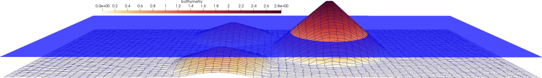
Figure 1: Well-balancing configuration with distorted mesh with 4225 ${\mathbb{Q}}_{1}$ degrees of freedom.

$I$	$\text{RK}(3,3;1)$	$\text{RK}(3,3;\tfrac{1}{3})$
4225	$1.33\text{\times}{10}^{-15}\text{\,}$	$9.44\text{\times}{10}^{-14}\text{\,}$
16641	$1.33\text{\times}{10}^{-15}\text{\,}$	$2.12\text{\times}{10}^{-13}\text{\,}$

Table 2: At-rest well-balancing results.

$I$	$\text{RK}(3,3;1)$	$\text{RK}(3,3;\tfrac{1}{3})$
513	$6.616\,751\,799\,797\,99\text{\times}{10}^{-14}\text{\,}$	$5.299\,568\,154\,477\,178\text{\times}{10}^{-13}\text{\,}$
1025	$1.642\,182\,047\,833\,548\text{\times}{10}^{-14}\text{\,}$	$6.257\,444\,144\,052\,46\text{\times}{10}^{-13}\text{\,}$

Table 3: Steady flow over inclined plane well-balancing results.

5.2.2 Steady flow over inclined plane with friction

We now test the well-balancing property for a steady flow over an inclined plane with Gauckler-Manning friction. The specific configuration that we consider is that proposed in Chertock et al. [13, Sec. 4.1] titled “Example 1” (Test 2). The domain is set to $D=(0,{\qty[scientific-notation=false,round-mode=figures,round-precision=5,drop-zero-decimal,round-pad=false]{25}{m}})$ with Dirichlet conditions on the left for inflow, and non-reflecting boundary conditions on the right for dynamic outflow. The topography profile is defined by $z(x)=-bx$. The unit discharge is initialized with $q(x)=q_{0}$. The initial and exact solution for the depth is given by $\mathsf{h}(x)\equiv\mathsf{h}_{0}=(\frac{n^{2}q_{0}^{2}}{b})^{3/10}$ where $n$ is the Gauckler-Manning friction coefficient. ; see (2.5) in [13], The coefficients are set to $b={\qty[scientific-notation=false,round-mode=figures,round-precision=5,drop-zero-decimal,round-pad=false]{0.01}{}},q_{0}={\qty[scientific-notation=false,round-mode=figures,round-precision=5,drop-zero-decimal,round-pad=false]{0.1}{m^{2}/s}},n={\qty[scientific-notation=false,round-mode=figures,round-precision=5,drop-zero-decimal,round-pad=false]{0.02}{m^{-1/3}s}}$ which gives approximately $\mathsf{h}_{0}\approx{\qty[scientific-notation=false,round-mode=figures,round-precision=5,drop-zero-decimal,round-pad=false]{0.0956352}{m}}$. We run until final time $T={\qty[scientific-notation=false,round-mode=figures,round-precision=5,drop-zero-decimal,round-pad=false]{100}{s}}$ with CFL 0.5 using $\text{RK}(3,3;1)$ and $\text{RK}(3,3;\tfrac{1}{3})$. We report the $\delta^{\infty}(T)$ error for two meshes in Table 3. Well-balancing is again achieved in this case.

5.2.3 Rainfall over inclined plane with friction

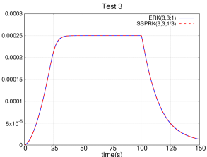
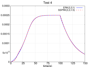
Figure 2: Comparison of discharge at outlet boundary ($x={\qty[scientific-notation=false,round-mode=figures,round-precision=5,drop-zero-decimal,round-pad=false]{2.5}{m}}$) for the “Test 3” and “Test 4” configurations from Table 2 in [13].

We now test the method’s ability to handle both rainfall and friction effects as sources. We again use the inclined plane bathymetry from the previous section, but now follow the configuration in [13, Sec. 4.1] titled “Example 3”. Here, the initial configuration is set to dry with a constant rain source $R(x)={\qty[scientific-notation=false,round-mode=figures,round-precision=5,drop-zero-decimal,round-pad=false]{1e-4}{ms^{-1}}}$ active in the interval $0\leq t\leq{\qty[scientific-notation=false,round-mode=figures,round-precision=5,drop-zero-decimal,round-pad=false]{100}{s}}$. The specific test cases we reproduce are “Test 3” and “Test 4” from Table 2 in [13]. The domain is set to $D=(0,{\qty[scientific-notation=false,round-mode=figures,round-precision=5,drop-zero-decimal,round-pad=false]{2.5}{m}})$ with slip conditions on the left and do nothing boundary conditions on the right. For both tests, we run until final time $T={\qty[scientific-notation=false,round-mode=figures,round-precision=5,drop-zero-decimal,round-pad=false]{150}{s}}$ with CFL 0.5 using $\text{RK}(3,3;1)$ and $\text{RK}(3,3;\tfrac{1}{3})$.The discharge was measured over time at the right boundary for the simulation for each test. We report the time history of the discharge in Figure 2. We observe comparable results to those reported in [13, Fig. 5]. For the $\text{RK}(3,3;\tfrac{1}{3})$ results in Test 4, there are some slight oscillations at the beginning of the simulation.

5.3 Convergence tests

In this section, we verify the accuracy of the proposed method. For the sake of brevity, we only report results in two space dimensions since we observe similar behavior in one space dimension.

5.3.1 Smooth vortex

$I$	$\text{RK}(3,3;1)$	rate	$\text{RK}(3,3;\tfrac{1}{3})$	rate
1089	$0.003\,578\,66$	-	$0.003\,572\,41$	-
4225	$0.000\,628\,104$	2.51	$0.000\,627\,444$	2.51
16641	$8.413\,59\text{\times}{10}^{-05}$	2.90	$8.399\,31\text{\times}{10}^{-05}$	2.90
66049	$1.095\,06\text{\times}{10}^{-05}$	2.94	$1.093\,53\text{\times}{10}^{-05}$	2.94
263169	$1.425\,12\text{\times}{10}^{-06}$	2.94	$1.424\,05\text{\times}{10}^{-06}$	2.94
1050625	$2.811\,45\text{\times}{10}^{-07}$	2.34	$1.918\,91\text{\times}{10}^{-07}$	2.89

Table 4: Error $\delta^{1}(T)$ and convergence rates for smooth vortex test with CFL 0.25.

We now demonstrate the convergence of the method with a smooth analytical solution of the Shallow Water Equations. This benchmark is a divergence-free vortex adapted (and slightly modified) from Ricchiuto and Bollermann [43, Sec. 2.3] which mimics geophysical flows [44]. Let $(\mathsf{h}_{\infty},{\bm{v}}_{\infty})$ be the far-field state. Then, the analytical solution is defined as follows:

(5.2a) $$\mathsf{h}({\bm{x}},t)=\mathsf{h}_{\infty}-\frac{1}{2gr_{0}^{2}}\psi(\overline{{\bm{x}}})^{2},$$

(5.2b) $${\bm{v}}:={\bm{v}}_{\infty}+\delta{\bm{v}},$$

(5.2c) $$\delta{\bm{v}}({\bm{x}},t):=\left(\partial_{x_{2}}\psi(\overline{{\bm{x}}}),-\partial_{x_{1}}\psi(\overline{{\bm{x}}})\right)^{\mathsf{T}},$$

with $\overline{{\bm{x}}}:={\bm{x}}-{\bm{x}}^{0}-{\bm{v}}_{\infty}t$ and $\psi({\bm{x}}):=\frac{\beta}{2\pi}\exp(\tfrac{1}{2}(1-\frac{\|{\bm{x}}\|^{2}_{\ell^{2}}}{r_{0}^{2}}))$. Here, ${\bm{x}}^{0}$ can be thought of as the center of the vortex, $\beta$ the vortex strength and $r_{0}$ the radius of the vortex. The parameters are set to $\mathsf{h}_{\infty}={\qty[scientific-notation=false,round-mode=figures,round-precision=5,drop-zero-decimal,round-pad=false]{2}{m}},\,\beta={\qty[scientific-notation=false,round-mode=figures,round-precision=5,drop-zero-decimal,round-pad=false]{2}{,}}\,r_{0}={\qty[scientific-notation=false,round-mode=figures,round-precision=5,drop-zero-decimal,round-pad=false]{1}{m}},\,{\bm{v}}_{\infty}=(1,1){\qty[scientific-notation=false,round-mode=figures,round-precision=5,drop-zero-decimal,round-pad=false]{}{ms^{-1}}}$. The computational domain is set to $D=(-6,{\qty[scientific-notation=false,round-mode=figures,round-precision=5,drop-zero-decimal,round-pad=false]{6}{m}})\times(-6,{\qty[scientific-notation=false,round-mode=figures,round-precision=5,drop-zero-decimal,round-pad=false]{6}{m}})$ with Dirichlet boundary conditions. We set the final time to $T={\qty[scientific-notation=false,round-mode=figures,round-precision=5,drop-zero-decimal,round-pad=false]{2}{s}}$. The time-stepping is performed with $\text{RK}(3,3;1)$ and $\text{RK}(3,3;\tfrac{1}{3})$ with CFL 0.25. We report the consolidated $\delta^{\infty}(T)$ error and rates in Table 4. We observe close to third order accuracy in time and space. The super-convergence in space is compatible with the theoretical result from [24, Prop. A.1].

5.3.2 Planar surface flow in paraboloid-shaped basin

$I$	$\text{RK}(3,3;1)$	rate	$\text{RK}(3,3;\tfrac{1}{3})$	rate
1089	$0.221\,698$	-	$0.226\,83$	-
4225	$0.063\,275\,9$	1.81	$0.064\,732\,7$	1.81
16641	$0.017\,227\,2$	1.88	$0.017\,851\,7$	1.86
66049	$0.005\,105\,51$	1.75	$0.005\,358\,52$	1.74
263169	$0.001\,740\,4$	1.55	$0.001\,834\,09$	1.55
1050625	$0.000\,704\,076$	1.31	$0.000\,738\,643$	1.31

Table 5: Error $\delta^{1}(T)$ and convergence rates for the test configuration with a planar surface flow in a paraboloid-shaped basin.

We now demonstrate the convergence of the method with Thacker’s planar surface flow in paraboloid-shaped basin [48]. The problem consists of a free-surface moving in a periodic motion inside a paraboloid-shaped basin.The moving shoreline is circular at all times. The precise configuration we use is the one introduced in Delestre et al. [15, Sec. 4.2.2] subsection “Planar surface in a paraboloid:” The computational domain is defined as $D=[0,{\qty[scientific-notation=false,round-mode=figures,round-precision=5,drop-zero-decimal,round-pad=false]{4}{m}}]\times[0,{\qty[scientific-notation=false,round-mode=figures,round-precision=5,drop-zero-decimal,round-pad=false]{4}{m}}]$ with slip boundary conditions. The theoretical period of the motion is $2\pi/\sqrt{2g\mathsf{h}_{0}}$ with $\mathsf{h}_{0}={\qty[scientific-notation=false,round-mode=figures,round-precision=5,drop-zero-decimal,round-pad=false]{0.1}{m}}$. The final time is three periods, approximately $T=\qty[round-mode=places,round-precision=8,scientific-notation=false]{13.45710440}{s}$. The time-stepping is performed with $\text{RK}(3,3;1)$ and $\text{RK}(3,3;\tfrac{1}{3})$ with CFL 0.5. We report the consolidated $\delta^{1}(T)$ error and rates in Table 5. We observe a convergence rate ranging from 1.8 to 1.3, which is consistent with what is reported in the literature.

5.4 Small-scale laboratory experiments

In this section, we simulate two small-scale laboratory experiments described in Martínez-Aranda et al. [39]. The goal of the experiments was to provide validation data for shallow water solvers by studying complex steady and transient flume experiments. The experiments comprised of transcritical steady flow and dam-break flow around obstacles and complex beds. In this paper, we reproduce cases “G2-S.2” and “G3-D.1” described in Sections 4.3.1 and 4.4.2 in [39], respectively. We refer the reader to [39] for a detailed description of the experimental configuration. The set up can also be found in the source code for the ryujin software.

5.4.1 G2-S.2

Figure 3: Top view representation for the “G2-S.2” test case.

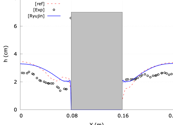
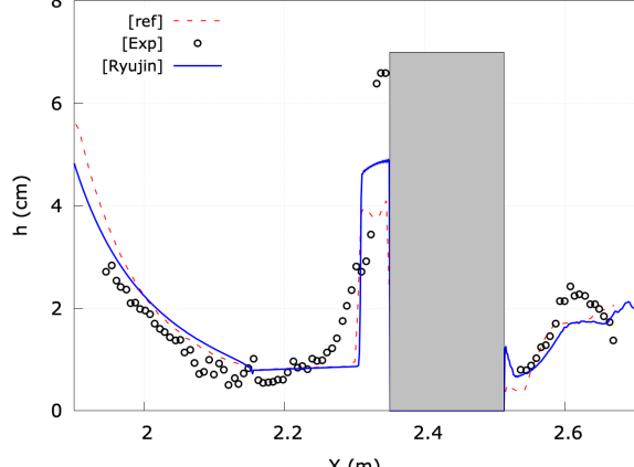
Figure 4: Time snapshots for “G2-S.2” showing water elevation and bathymetry.

Figure 5: Comparison of numerically computed water depth (solid blue line) for the “G2-S.2” configuration along the two sections with experimental data (black circles) and corresponding simulation data from [39] (red dashed line).

The “G2-S.2” test case consists of a steady inflow discharge of ${\mathsf{Q}}_{0}={\qty[scientific-notation=false,round-mode=figures,round-precision=5,drop-zero-decimal,round-pad=false]{9.01}{m^{3}/h}}$ with the flume containing a semi-circular bump across its width followed by a rectangular obstacle placed at the center line of the flume. We give a top view representation of the set up in Figure 5. Note that the discharge here is the volumetric flow rate. For our simulation, we use the unit flow discharge $q_{0}={\mathsf{Q}}_{0}/{\qty[scientific-notation=false,round-mode=figures,round-precision=5,drop-zero-decimal,round-pad=false]{0.24}{m}}$ which gives $q_{0}={\qty[scientific-notation=false,round-mode=figures,round-precision=5,drop-zero-decimal,round-pad=false]{0.0104}{m^{2}/s}}$ (here, the ${\qty[scientific-notation=false,round-mode=figures,round-precision=5,drop-zero-decimal,round-pad=false]{0.24}{m}}$ corresponds to the flume width). We reproduce this case using the computational domain $D=[0,{\qty[scientific-notation=false,round-mode=figures,round-precision=5,drop-zero-decimal,round-pad=false]{6.078}{m}}]\times[-0.12,{\qty[scientific-notation=false,round-mode=figures,round-precision=5,drop-zero-decimal,round-pad=false]{0.12}{m}}]$ with 928137 ${\mathbb{Q}}_{1}$ degrees of freedom (this corresponds to the mesh-size being roughly [scientific-notation=false, round-mode=figures,round-precision = 5, drop-zero-decimal, round-pad = false]1.25mm in each direction). Note that we omit discretizing the tank reservoir since it is not needed for simulating steady inflow. The initial set up consists of a dry flume where the bottom/top boundaries are set to slip boundary conditions and the right boundary is set to non-reflecting boundary conditions for dynamic outflow. On the left boundary, we enforce the steady inflow discharge and do nothing boundary conditions for the water depth. We run the simulation with $\text{RK}(4,3;1)$ until $T={\qty[scientific-notation=false,round-mode=figures,round-precision=5,drop-zero-decimal,round-pad=false]{50}{s}}$ with CFL 0.9 to allow the flow to reach a steady state. We output four time snapshots for $t=\{$15\text{\,}\mathrm{s}$,$30\text{\,}\mathrm{s}$,$50\text{\,}\mathrm{s}$\}$ in Figure 5.

In the experiments, the water depth was measured at two different sections: $x={\qty[scientific-notation=false,round-mode=figures,round-precision=5,drop-zero-decimal,round-pad=false]{2.40}{m}}$ (across width of flume spanning the rectangular obstacle) and $y={\qty[scientific-notation=false,round-mode=figures,round-precision=5,drop-zero-decimal,round-pad=false]{0}{m}}$ (centerline of the flume). In Figure 5, we compare the numerical output of our simulations along the sections and compare with the experimental data as well as the simulation data reported in [39]. Overall, our simulation compares well with the experiments and simulations from [39]. The discrepancies between the numerical simulations are due to mesh resolution differences. The discrepancies with the experiments show the shortcomings of the shallow water equations and that, short to solving the Navier-Stokes equations, a higher-fidelity model is required.

5.4.2 G3-D.1

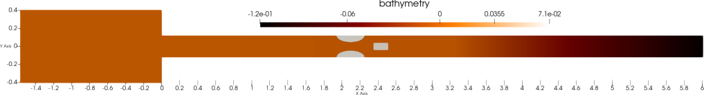
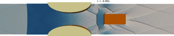
Figure 6: Top view representation for “G3-D.1” case.

Figure 7: Time snapshots for “G3-D.1” showing water elevation and bathymetry.

The case “G3-D.1” consists of a dam-break flow with height ${\mathsf{H}}_{0}={\qty[scientific-notation=false,round-mode=figures,round-precision=5,drop-zero-decimal,round-pad=false]{0.055}{m}}$ in the reservoir and the flume containing two semi-circular Venturi constriction elements followed by rectangular obstacle placed at the center line of the flume. We give a top view representation of the set up in Figure 7. We reproduce this case using the computation domain $D=D_{\text{res}}\cup D_{\text{flume}}$ where $D_{\text{res}}=[-1.58,{\qty[scientific-notation=false,round-mode=figures,round-precision=5,drop-zero-decimal,round-pad=false]{0}{m}}]\times[-0.405,{\qty[scientific-notation=false,round-mode=figures,round-precision=5,drop-zero-decimal,round-pad=false]{0.405}{m}}]$ and $D_{\text{flume}}=[0,{\qty[scientific-notation=false,round-mode=figures,round-precision=5,drop-zero-decimal,round-pad=false]{6.078}{m}}]\times[-0.12,{\qty[scientific-notation=false,round-mode=figures,round-precision=5,drop-zero-decimal,round-pad=false]{0.12}{m}}]$ with 1753793 ${\mathbb{Q}}_{1}$ degrees of freedom (this corresponds to the mesh-size being roughly [scientific-notation=false, round-mode=figures,round-precision = 5, drop-zero-decimal, round-pad = false]1.25mm in each direction). The flume is initially dry. The slip boundary condition is enforced on all the boundaries except the right-most one. Non-reflecting boundary conditions are enforced on the right boundary for dynamic outflow. We run the simulation with $\text{RK}(4,3;1)$ until $T={\qty[scientific-notation=false,round-mode=figures,round-precision=5,drop-zero-decimal,round-pad=false]{20}{s}}$ with CFL 0.9. We output four time snapshots of the water elevation for $t=\{$3\text{\,}\mathrm{s}$,$4\text{\,}\mathrm{s}$,$5\text{\,}\mathrm{s}$,$6\text{\,}\mathrm{s}$\}$ in Figure 7.

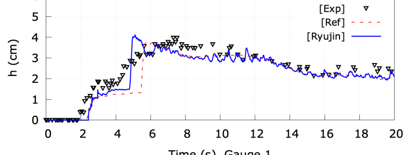
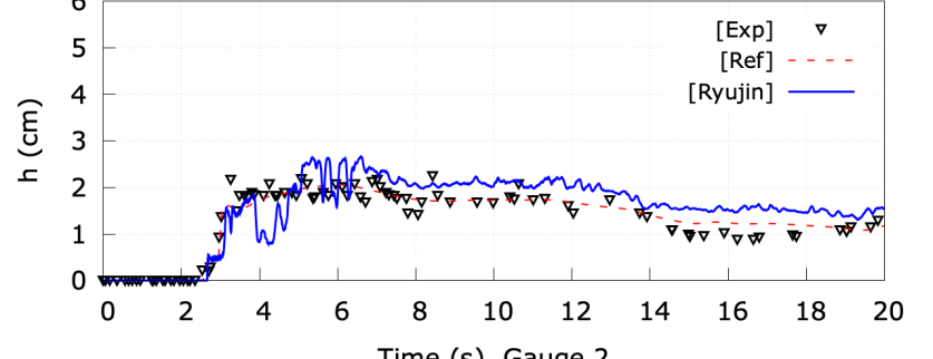
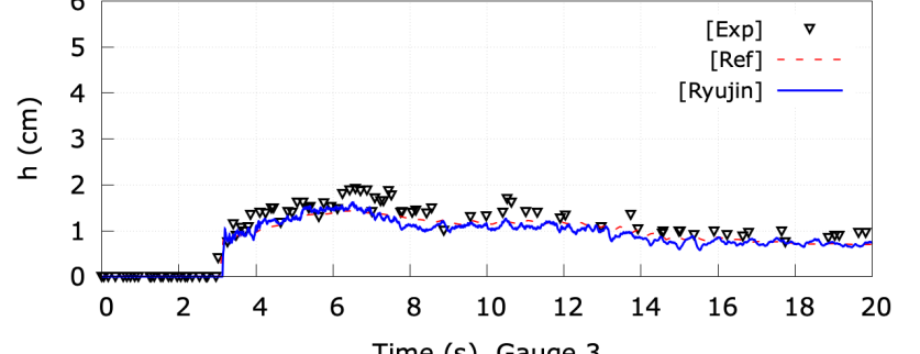
Figure 8: Temporal series over $t\in[0,{\qty[scientific-notation=false,round-mode=figures,round-precision=5,drop-zero-decimal,round-pad=false]{20}{s}}]$ comparing numerical water depth (blue solid line), experimental data (black triangles) and simulation data from [39] (red dashed line). From top to bottom: Gauge 1, Gauge 2, Gauge 3.

Method	# cycles	throughput	runtime
$\text{RK}(2,2;\tfrac{1}{2})$	1019	[scientific-notation=false, round-mode=figures,round-precision = 5, drop-zero-decimal, round-pad = false]1.3564 MQ/s	[scientific-notation=false, round-mode=figures,round-precision = 5, drop-zero-decimal, round-pad = false]99.64s
$\text{RK}(2,2;1)$	510	[scientific-notation=false, round-mode=figures,round-precision = 5, drop-zero-decimal, round-pad = false]1.2762 MQ/s	[scientific-notation=false, round-mode=figures,round-precision = 5, drop-zero-decimal, round-pad = false]52.99s
$\text{RK}(3,3;\tfrac{1}{3})$	1019	[scientific-notation=false, round-mode=figures,round-precision = 5, drop-zero-decimal, round-pad = false]1.3578 MQ/s	[scientific-notation=false, round-mode=figures,round-precision = 5, drop-zero-decimal, round-pad = false]149.20s
$\text{RK}(3,3;1)$	340	[scientific-notation=false, round-mode=figures,round-precision = 5, drop-zero-decimal, round-pad = false]1.2511 MQ/s	[scientific-notation=false, round-mode=figures,round-precision = 5, drop-zero-decimal, round-pad = false]54.01s
$\text{RK}(4,3;1)$	255	[scientific-notation=false, round-mode=figures,round-precision = 5, drop-zero-decimal, round-pad = false]1.2312 MQ/s	[scientific-notation=false, round-mode=figures,round-precision = 5, drop-zero-decimal, round-pad = false]54.91s
$\text{RK}(5,4;1)$	204	[scientific-notation=false, round-mode=figures,round-precision = 5, drop-zero-decimal, round-pad = false]1.1494 MQ/s	[scientific-notation=false, round-mode=figures,round-precision = 5, drop-zero-decimal, round-pad = false]58.79s

Table 6: Efficiency comparison of various time-stepping schemes. We report the total number of cycles for a full Runge-Kutta step to reach final time $T={\qty[scientific-notation=false,round-mode=figures,round-precision=5,drop-zero-decimal,round-pad=false]{0.5}{s}}$ with CFL 0.2, the average throughput measured in million $Q_{1}$-mesh points per second (MQ/s) for a single Runge-Kutta substep (consisting of a single forward Euler step) and the total runtime to reach the final simulation time.

In the experiments reported in [39], three wave gauges were placed in the basin to measure the water depth over the duration of the experiment. The specific locations of the gauges are given by: “Gauge 1” $({\qty[scientific-notation=false,round-mode=figures,round-precision=5,drop-zero-decimal,round-pad=false]{225}{cm}},{\qty[scientific-notation=false,round-mode=figures,round-precision=5,drop-zero-decimal,round-pad=false]{12}{cm}})$; “Gauge 2” $({\qty[scientific-notation=false,round-mode=figures,round-precision=5,drop-zero-decimal,round-pad=false]{240}{cm}},{\qty[scientific-notation=false,round-mode=figures,round-precision=5,drop-zero-decimal,round-pad=false]{20}{cm}})$; “Gauge 3” $({\qty[scientific-notation=false,round-mode=figures,round-precision=5,drop-zero-decimal,round-pad=false]{260}{cm}},{\qty[scientific-notation=false,round-mode=figures,round-precision=5,drop-zero-decimal,round-pad=false]{12}{cm}})$. In Figure 8, we compare the numerical output of our simulations with the experimental data and the simulation data reported in [39]. Overall, our simulation compares well with the experiment and simulations from [39].

5.5 Efficiency tests

We now report a quick efficiency test to compare various time-stepping techniques. We choose the smooth vortex benchmark described in 5.3.1 and run until final time $T={\qty[scientific-notation=false,round-mode=figures,round-precision=5,drop-zero-decimal,round-pad=false]{0.5}{s}}$ with CFL 0.2 with the mesh composed of 66,049 ${\mathbb{Q}}_{1}$ degrees of freedom. Each simulation is performed on a single rank and single thread on a laptop computer. In Table 6, we report the results of our tests. We see that the overall efficiency of each method is directly proportional to the efficiency coefficient $c_{\text{eff}}$.

5.6 High-fidelity simulation

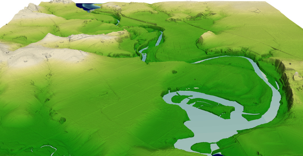
(a)

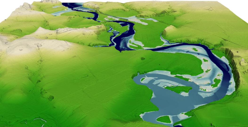
(b)

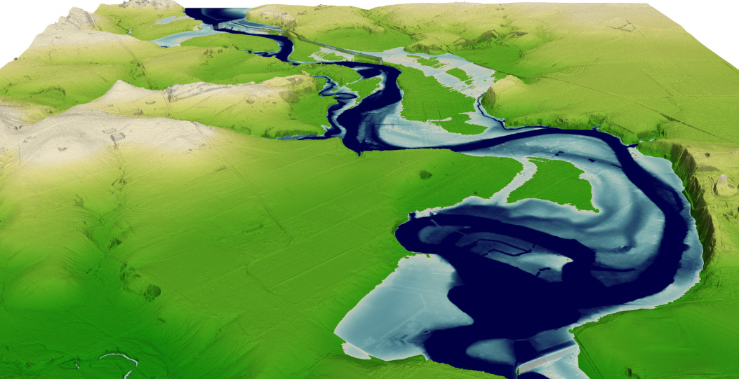
(c)

Figure 9: Temporal snapshots for the high-fidelity simulation of a dam break with $58{,}735{,}617$ ${\mathbb{Q}}_{1}$ degrees of freedom per component. The figures show a three dimensional rendering of the bathymetry $z({\bm{x}})$ with a color scale ranging from dark green to light ocre, and the water surface $\mathsf{h}+z$ with a color scale ranging from dark blue (large $\mathsf{h}$) to light blue (small $\mathsf{h}$). The vertical direction is scaled by a factor 10.

Lastly we perform a high-fidelity dam break simulation with the shallow water equations using realistic topography data. To this end we linked the ryujin software to the Geospatial Data Abstraction Library (GDAL) in order to read in digital elevation models (DEMs). The DEM considered here was obtained from the United States Geological Survey 3D Elevation Program United States Geological Survey [49] via OpenTopography and shows a portion of Lake Dunlap and the Guadalupe river in the state of Texas with a spatial resolution of ${\qty[scientific-notation=false,round-mode=figures,round-precision=5,drop-zero-decimal,round-pad=false]{1}{m}}\times{\qty[scientific-notation=false,round-mode=figures,round-precision=5,drop-zero-decimal,round-pad=false]{1}{m}}$. We simulate the breaking of the dam at Lake Dunlap. The simulation was performed on the computational domain $D=[0,{\qty[scientific-notation=false,round-mode=figures,round-precision=5,drop-zero-decimal,round-pad=false]{7168}{m}}]\times[0,{\qty[scientific-notation=false,round-mode=figures,round-precision=5,drop-zero-decimal,round-pad=false]{8192}{m}}]$ which is the bounding box for the DEM data until final time $T=$2\text{\,}\mathrm{h}$$. We use a Gauckler-Manning’s friction source term with a roughness coefficient of $n={\qty[scientific-notation=false,round-mode=figures,round-precision=5,drop-zero-decimal,round-pad=false]{0.025}{m^{-1/3}s}}$ and a gravity constant of $g={\qty[scientific-notation=false,round-mode=figures,round-precision=5,drop-zero-decimal,round-pad=false]{9.81}{ms^{-2}}}$. We set up an initial water column with $\mathsf{h}+z={\qty[scientific-notation=false,round-mode=figures,round-precision=5,drop-zero-decimal,round-pad=false]{179.5}{m}}$ (above sea level) for the upper basin and $\mathsf{h}+z={\qty[scientific-notation=false,round-mode=figures,round-precision=5,drop-zero-decimal,round-pad=false]{163.5}{m}}$ slowly sloping down to ${\qty[scientific-notation=false,round-mode=figures,round-precision=5,drop-zero-decimal,round-pad=false]{161.3}{m}}$ for the river bed; both with zero initial velocity. On the northern boundary of the domain we enforce Dirichlet conditions with $\mathsf{h}+z={\qty[scientific-notation=false,round-mode=figures,round-precision=5,drop-zero-decimal,round-pad=false]{182.5}{m}}$ which ensure that the upper basin is always filled. We emphasize that we chose this flow configuration purely for demonstration purposes and that it is not particularly realistic: we do not factor in the finite amount of water stored in the upper basin (as it is in fact not fully simulated); we make no attempt of creating a realistic initial configuration of the downstream river with correct water height and stream velocity; and the DEM does not contain bathymetry information of the river bed.

The computation was performed with $58{,}735{,}617$ ${\mathbb{Q}}_{1}$ degrees of freedom per component on 768 ranks (and 2 threads per rank) on the Whistler cluster at Texas A&M University using single-precision floating point arithmetic. We performed $152{,}637$ $\text{RK}(3,3;1)$ steps with a chosen CFL number of 0.9 resulting in an average time step size of ${\tau}_{\text{ERK}}\approx{\qty[scientific-notation=false,round-mode=figures,round-precision=5,drop-zero-decimal,round-pad=false]{4.72e-02}{s}}$. The total CPU time summed over all ranks was about [scientific-notation=false, round-mode=figures,round-precision = 5, drop-zero-decimal, round-pad = false]9820h with an average per-rank throughput of about ${\qty[scientific-notation=false,round-mode=figures,round-precision=5,drop-zero-decimal,round-pad=false]{1.52}{MQ/s}}$, where MQ/s stands for million ${\mathbb{Q}}_{1}$-mesh point updates per second for a single Runge-Kutta substep (consisting of a single forward-Euler step). We recorded a total runtime of approximately ${\qty[scientific-notation=false,round-mode=figures,round-precision=5,drop-zero-decimal,round-pad=false]{6.43}{h}}$ (wall time) which equates to a combined throughput over all ranks of about ${\qty[scientific-notation=false,round-mode=figures,round-precision=5,drop-zero-decimal,round-pad=false]{1159.25}{MQ/s}}$.

We visualize in Figure 9 the simulation results for temporal snapshots at initial time $t={\qty[scientific-notation=false,round-mode=figures,round-precision=5,drop-zero-decimal,round-pad=false]{0}{h}}$, at $t={\qty[scientific-notation=false,round-mode=figures,round-precision=5,drop-zero-decimal,round-pad=false]{1}{h}}$, and at $t={\qty[scientific-notation=false,round-mode=figures,round-precision=5,drop-zero-decimal,round-pad=false]{2}{h}}$. The figure shows a three dimensional rendering of the bathymetry $z({\bm{x}})$ with a color scale ranging from dark green to light ocre where the bathymetry is scaled by a factor 10. Similarly, the water surface $\mathsf{h}+z$ is overlayed with the same scaling factor and with a color scale ranging from dark blue to light blue for large to small values of $\mathsf{h}$.

6 Conclusion

In this work, we provided a high-order space and time approximation of the shallow water equations with external sources on unstructured meshes. The numerical method was shown to be invariant-domain preserving and well-balanced with respect to rest states whether the shoreline is aligned with the mesh or not. The method was also shown to be robust with respect to external source terms. This work will be the stepping stone for various multi-physics extensions of the shallow water equations like the Serre-Green-Naghdi Equations which account for dispersive water waves or subsurface models such as Richard’s equation.

Data availability statement

A high performance implementation of the algorithms discussed in this paper are freely available as part of the ryujin project [38, 30]. The source code repository is located at https://github.com/conservation-laws/ryujin. Parameter and configuration files for the numerical illustrations reported in Section 5 are made available upon request.

Appendix A Boundary conditions

In this section, we describe how the boundary conditions are enforced for the IDP explicit Runge-Kutta schemes above. Recall that the Shallow Water Equations with flat topography (and no external source terms) are equivalent to the isentropic compressible Euler Equations when the adiabatic index $\gamma$ is 2. Thus, the details in this section are a direct modification of the work seen in [30] where it is shown how to enforce “reflecting” (i.e., slip or wall) and “non-reflecting” boundary conditions for the isentropic Euler Equations.

A.1 Preliminaries

Boundary conditions are enforced by post-processing the approximation at the end of each stage of the ERK-IDP algorithm. We consider two types of boundary conditions: (i) Reflecting conditions, also called “slip” or “wall”: ${\bm{v}}{\cdot}{\bm{n}}=0$; (ii) Non-reflecting conditions. Let $\partial D_{\textup{r}}\subset\partial D$ be the boundary where reflecting conditions are enforced. Let $\partial D_{\textup{nr}}$ denote the complement of $\partial D_{\textup{r}}$ in $\partial D$ where non-reflecting conditions will be enforced. Let ${\mathcal{V}}_{\textup{r}}^{\partial}\subset{\mathcal{V}}^{\partial}$ be the collection of all the boundary degrees of freedom $i$ such that $\varphi_{i|\partial D_{\textup{r}}}\not\equiv 0$. Let ${\mathcal{V}}^{\partial}_{\textup{r}}\subset{\mathcal{V}}^{\partial}$ be the collection of all boundary degrees of freedom $i$ such that $\varphi_{i|\partial D_{\textup{nr}}}\not\equiv 0$. We define the normal vectors associated with the degrees of freedom in ${\mathcal{V}}_{\textup{r}}^{\partial}$ and ${\mathcal{V}}_{\textup{nr}}^{\partial}$, respectively:

(A.1) $${\bm{n}}_{i}^{\textup{r}}:=\frac{\int_{\partial D_{\textup{r}}}\varphi_{i}{\bm{n}}\,{\mathrm{d}}s}{\|\int_{\partial D_{\textup{r}}}\varphi_{i}{\bm{n}}\,{\mathrm{d}}s\|_{\ell^{2}}},\qquad{\bm{n}}_{i}^{\textup{nr}}:=\frac{\int_{\partial D_{\textup{nr}}}\varphi_{i}{\bm{n}}\,{\mathrm{d}}s}{\|\int_{\partial D_{\textup{nr}}}\varphi_{i}{\bm{n}}\,{\mathrm{d}}s\|_{\ell^{2}}}.$$

In the following two sections, the symbol U denotes the state obtained at the end of each stage. The post-processed state is denoted by $\textsf{{U}}^{\textup{P}}$.

A.2 Reflecting boundary conditions

Let $i\in{\mathcal{V}}_{\textup{r}}^{\partial}$ and let $\textsf{{U}}_{i}=({\mathsf{H}}_{i},\textsf{{Q}}_{i})^{\mathsf{T}}$. Reflecting boundary conditions are enforced at the $i$-th degree of freedom by setting:

(A.2) $$\textsf{{U}}_{i}^{\textup{P}}:=({\mathsf{H}}_{i},\textsf{{Q}}_{i}-(\textsf{{Q}}_{i}{\cdot}{\bm{n}}_{i}^{\text{r}}){\bm{n}}_{i}^{\text{r}})^{\mathsf{T}}.$$

A.3 Non-reflecting boundary conditions

We now consider non-reflecting boundary conditions at $i\in{\mathcal{V}}_{\textup{nr}}^{\partial}$ based on Riemann invariants. We note that the idea of working with the Riemann invariants of the Shallow Water Equations for the use of boundary conditions is a common approach in the literature (see: Bristeau and Coussin [9, Sec. 6]). For notational simplicity, we assume the following states are at the $i$-th degree of freedom and drop the subscript notation. Here, ${\bm{n}}:={\bm{n}}_{i}^{\textup{nr}}$.

Let $\mathsf{h}:=\mathsf{h}(\textsf{{U}}),\,\textsf{{Q}}:={\bm{q}}(\textsf{{U}})$ and set:

(A.3) $$\textsf{{V}}:=\mathsf{h}^{-1}\textsf{{Q}},\qquad{\mathsf{V}}_{n}:=\textsf{{V}}{\cdot}{\bm{n}},\qquad\textsf{{V}}^{\perp}:=\textsf{{V}}-(\textsf{{V}}{\cdot}{\bm{n}}){\cdot}{\bm{n}},\qquad a:=\sqrt{g\mathsf{h}}.$$

Assume that the topography is flat and that there are no external source terms. Then, the characteristic variables and characteristic speeds for the one-dimensional system, $\partial_{t}{\bm{u}}+\partial_{x}({\mathbbm{f}}({\bm{u}}){\bm{n}})=0$, are:

(A.4) $$\underbrace{\begin{cases}\lambda_{1}(\textsf{{U}},{\bm{n}}):={\mathsf{V}}_{n}-a\\ {\mathsf{R}}_{1}(\textsf{{U}},{\bm{n}}):={\mathsf{V}}_{n}-2a,\end{cases}}_{\text{multiplicity }1}\qquad\underbrace{\begin{cases}\lambda_{2}(\textsf{{U}},{\bm{n}}):={\mathsf{V}}_{n}\\ \textsf{{V}}^{\perp},\end{cases}}_{\text{multiplicity }d-1}\qquad\underbrace{\begin{cases}\lambda_{3}(\textsf{{U}},{\bm{n}}):={\mathsf{V}}_{n}+a\\ {\mathsf{R}}_{3}(\textsf{{U}},{\bm{n}}):={\mathsf{V}}_{n}+2a.\end{cases}}_{\text{multiplicity }1}$$

Note in passing there are only two Riemann invariants for the Shallow Water Equations, but we use the notation ${\mathsf{R}}_{1}$ and ${\mathsf{R}}_{3}$ so that they correspond directly to the eigenvalues. We consider four different cases depending on the type of flow at the boundary:

• torrential inflow: $\hskip 8.0pt{\mathsf{V}}_{n}<0\text{ and }a<|{\mathsf{V}}_{n}|\qquad\lambda_{1}\leq\lambda_{2}\leq\lambda_{3}<0$,

• torrential outflow: $\hskip 4.0pt0\leq{\mathsf{V}}_{n}\text{ and }a\leq|{\mathsf{V}}_{n}|\qquad 0\leq\lambda_{1}\leq\lambda_{2}\leq\lambda_{3}$,

• fluvial inflow:$\hskip 27.0pt{\mathsf{V}}_{n}<0\text{ and }|{\mathsf{V}}_{n}|<a\qquad\lambda_{1}\leq\lambda_{2}<0\leq\lambda_{3}$,

• fluvial outflow: $\hskip 17.0pt0\leq{\mathsf{V}}_{n}\text{ and }a<|{\mathsf{V}}_{n}|\qquad\lambda_{1}<0\leq\lambda_{2}\leq\lambda_{3}$.
  

Note that the nomenclature “torrential” is equivalent to “supersonic” and “fluvial” is equivalent to “subsonic” in the context of gas dynamics. We assume that outside the domain $D$, we have at hand some Dirichlet data $\textsf{{U}}^{\textup{D}}:=(\mathsf{h}^{\textup{D}},\textsf{{Q}}^{\textup{D}})^{\mathsf{T}}$. Just as in [30], we are going to postprocess the solution U so that the characteristic variables of the post-processed state $\textsf{{U}}^{\textup{P}}$ associated with the in-coming eigenvalues match those of the prescribed Dirichlet data $\textsf{{U}}^{\textup{D}}$, while leaving the out-going characteristics unchanged. More precisely, the strategy consists of finding $\textsf{{U}}^{\textup{P}}$ so that the following holds:

(A.5a) $${\mathsf{R}}_{l}(\textsf{{U}}^{\textup{P}})=\begin{cases}{\mathsf{R}}_{l}(\textsf{{U}}^{\textup{D}})&\text{if }\lambda_{l}(\textsf{{U}},{\bm{n}}^{\textup{nr}})<0,\\ {\mathsf{R}}_{l}(\textsf{{U}})&\text{if }0\leq\lambda_{l}(\textsf{{U}},{\bm{n}}^{\textup{nr}}),\end{cases}\quad l\in\{1,3\},$$

(A.5b) $$(\textsf{{V}}^{\textup{P}})^{\perp}=\begin{cases}(\textsf{{V}}^{\textup{D}})^{\perp}&\text{if }\lambda_{2}(\textsf{{U}},{\bm{n}}^{\textup{nr}})<0,\\ \textsf{{V}}^{\perp}&\text{if }0\leq\lambda_{2}(\textsf{{U}},{\bm{n}}^{\textup{nr}}).\end{cases}$$

We now solve the above system for each of the four flow configurations mentioned above.
Torrential inflow: Assume that $\lambda_{1}(\textsf{{U}},{\bm{n}})\leq\lambda_{2}(\textsf{{U}},{\bm{n}})\leq\lambda_{3}(\textsf{{U}},{\bm{n}})<0$. Since all the characteristics are entering the computational domain, the postprocessing consists of replacing U by $\textsf{{U}}^{\textup{D}}$:

(A.6) $$\textsf{{U}}^{\textup{P}}=\textsf{{U}}^{\textup{D}}.$$

Torrential outflow: Assume that $0\leq\lambda_{1}(\textsf{{U}},{\bm{n}})\leq\lambda_{2}(\textsf{{U}},{\bm{n}})\leq\lambda_{3}(\textsf{{U}},{\bm{n}})$. Since all the characteristics are exiting the computational domain, the postprocessing consists of doing nothing:

(A.7) $$\textsf{{U}}^{\textup{P}}=\textsf{{U}}.$$

Fluvial inflow: Assume that $\lambda_{1}(\textsf{{U}},{\bm{n}})\leq\lambda_{2}(\textsf{{U}},{\bm{n}})<0<\lambda_{3}(\textsf{{U}},{\bm{n}})$. Then, $\textsf{{U}}^{\textup{P}}$ is obtained by solving the following system:

(A.8) $${\mathsf{R}}_{1}(\textsf{{U}}^{\textup{P}})={\mathsf{R}}_{1}(\textsf{{U}}^{\textup{D}}),\qquad(\textsf{{V}}^{\textup{P}})^{\perp}=(\textsf{{V}}^{\textup{D}})^{\perp},\qquad{\mathsf{R}}_{3}(\textsf{{U}}^{\textup{P}})={\mathsf{R}}_{3}(\textsf{{U}}).$$

This gives that ${\mathsf{V}}_{n}^{\textup{P}}=\frac{1}{2}\left({\mathsf{R}}_{1}(\textsf{{U}}^{\textup{D}})+{\mathsf{R}}_{3}(\textsf{{U}})\right)$ and $4a^{\textup{P}}=\left({\mathsf{R}}_{3}(\textsf{{U}})-{\mathsf{R}}_{1}(\textsf{{U}}^{\textup{D}})\right)={\mathsf{V}}_{n}+2a-({\mathsf{V}}_{n}^{\textup{D}}-2a^{\textup{D}})$. Since in this flow configuration ${\mathsf{V}}_{n}+2a>0$, for $a^{\textup{P}}$ to be positive it must be that: ${\mathsf{V}}_{n}^{\textup{D}}\leq 2a^{\textup{D}}$ which is an admissibility condition on the Dirichlet data. Finally, the postprocessing for a fluvial inflow boundary condition consists of setting the solution $\textsf{{U}}^{\textup{P}}$ to:

(A.9a) $$\mathsf{h}^{\textup{P}}=\frac{1}{g}(a^{\textup{P}})^{2}=\frac{1}{g}\left(\frac{{\mathsf{R}}_{3}(\textsf{{U}})-{\mathsf{R}}_{1}(\textsf{{U}}^{\textup{D}})}{4}\right)^{2},$$

(A.9b) $$\textsf{{Q}}^{\textup{P}}=\mathsf{h}^{\textup{P}}\times\left((\textsf{{V}}^{\textup{D}})^{\perp}+{\mathsf{V}}_{n}^{\textup{P}}{\bm{n}}\right),\quad\text{ with }\quad{\mathsf{V}}_{n}^{\textup{P}}=\frac{1}{2}\left({\mathsf{R}}_{1}(\textsf{{U}}^{\textup{D}})+{\mathsf{R}}_{3}(\textsf{{U}})\right).$$

Fluvial outflow: Assume that $\lambda_{1}(\textsf{{U}},{\bm{n}})<0<\lambda_{2}(\textsf{{U}},{\bm{n}})<\lambda_{3}(\textsf{{U}},{\bm{n}})$. Then, $\textsf{{U}}^{\textup{P}}$ is obtained by solving the following system:

(A.10) $${\mathsf{R}}_{1}(\textsf{{U}}^{\textup{P}})={\mathsf{R}}_{1}(\textsf{{U}}^{\textup{D}}),\qquad(\textsf{{V}}^{\textup{P}})^{\perp}=\textsf{{V}}^{\perp},\qquad{\mathsf{R}}_{3}(\textsf{{U}}^{\textup{P}})={\mathsf{R}}_{3}(\textsf{{U}}).$$

Notice now that only one Dirichlet condition is prescribed on the first characteristic since $\lambda_{1}<0$. Again, we have that ${\mathsf{V}}_{n}^{\textup{P}}=\frac{1}{2}\left({\mathsf{R}}_{1}(\textsf{{U}}^{\textup{D}})+{\mathsf{R}}_{3}(\textsf{{U}})\right)$ and $4a^{\textup{P}}=\left({\mathsf{R}}_{3}(\textsf{{U}})-{\mathsf{R}}_{1}(\textsf{{U}}^{\textup{D}})\right)$. We also have the same admissibility condition on the Dirichlet data: ${\mathsf{V}}_{n}^{\textup{D}}\leq 2a^{\textup{D}}$ for $a^{\textup{P}}>0$. Finally, the postprocessing for a fluvial outflow boundary condition consists of setting the solution $\textsf{{U}}^{\textup{P}}$ to:

(A.11a) $$\mathsf{h}^{\textup{P}}=\frac{1}{g}(a^{\textup{P}})^{2}=\frac{1}{g}\left(\frac{{\mathsf{R}}_{3}(\textsf{{U}})-{\mathsf{R}}_{1}(\textsf{{U}}^{\textup{D}})}{4}\right)^{2},$$

(A.11b) $$\textsf{{Q}}^{\textup{P}}=\mathsf{h}^{\textup{P}}\times\left(\textsf{{V}}^{\perp}+{\mathsf{V}}_{n}^{\textup{P}}{\bm{n}}\right),\quad\text{ with }\quad{\mathsf{V}}_{n}^{\textup{P}}=\frac{1}{2}\left({\mathsf{R}}_{1}(\textsf{{U}}^{\textup{D}})+{\mathsf{R}}_{3}(\textsf{{U}})\right).$$

Remark A.1 (Conservation and admissibility).

The conservation and admissibility properties of the proposed boundary conditions are described in [30, Sec. 4.3.3]. $\square$

References

• Arndt et al. [2023] D. Arndt, W. Bangerth, M. Bergbauer, M. Feder, M. Fehling, J. Heinz, T. Heister, L. Heltai, M. Kronbichler, M. Maier, P. Munch, J.-P. Pelteret, B. Turcksin, D. Wells, and S. Zampini. The deal.II library, version 9.5. Journal of Numerical Mathematics, 31(3):231–246, 2023.
• Audusse and Bristeau [2005] E. Audusse and M.-O. Bristeau. A well-balanced positivity preserving “second-order” scheme for shallow water flows on unstructured meshes. J. Comput. Phys., 206(1):311–333, 2005.
• Audusse et al. [2004] E. Audusse, F. Bouchut, M.-O. Bristeau, R. Klein, and B. Perthame. A fast and stable well-balanced scheme with hydrostatic reconstruction for shallow water flows. SIAM J. Sci. Comput., 25(6):2050–2065, 2004.
• Azerad et al. [2017] P. Azerad, J.-L. Guermond, and B. Popov. Well-balanced second-order approximation of the shallow water equation with continuous finite elements. SIAM J. Numer. Anal., 55(6):3203–3224, 2017.
• Bermúdez and Vázquez [1994] A. Bermúdez and M. E. Vázquez. Upwind methods for hyperbolic conservation laws with source terms. Comput. Fluids, 23(8):1049–1071, 1994.
• Bollermann et al. [2011] A. Bollermann, S. Noelle, and M. Lukáčová-Medvidová. Finite volume evolution Galerkin methods for the shallow water equations with dry beds. Commun. Comput. Phys., 10(2):371–404, 2011.
• Boris and Book [1997] J. P. Boris and D. L. Book. Flux-corrected transport. Journal of computational physics, 135(2):172–186, 1997.
• Bouchut [2004] F. Bouchut. Nonlinear stability of finite volume methods for hyperbolic conservation laws and well-balanced schemes for sources. Frontiers in Mathematics. Birkhäuser Verlag, Basel, 2004.
• Bristeau and Coussin [2001] M.-O. Bristeau and B. Coussin. Boundary conditions for the shallow water equations solved by kinetic schemes. Research Report inria-00072305, INRIA, 2001.
• Brodtkorb et al. [2012] A. R. Brodtkorb, M. L. Sa.e.tra, and M. Altinakar. Efficient shallow water simulations on gpus: Implementation, visualization, verification, and validation. Computers & Fluids, 55:1–12, 2012.
• Castro and Semplice [2019] M. J. Castro and M. Semplice. Third-and fourth-order well-balanced schemes for the shallow water equations based on the cweno reconstruction. International Journal for Numerical Methods in Fluids, 89(8):304–325, 2019.
• Caviedes-Voullième et al. [2023] D. Caviedes-Voullième, M. Morales-Hernández, M. R. Norman, and I. Özgen-Xian. SERGHEI (SERGHEI-SWE) v1.0: a performance-portable high-performance parallel-computing shallow-water solver for hydrology and environmental hydraulics. Geoscientific Model Development, 16(3):977–1008, 2023.
• Chertock et al. [2015] A. Chertock, S. Cui, A. Kurganov, and T. Wu. Well-balanced positivity preserving central-upwind scheme for the shallow water system with friction terms. Internat. J. Numer. Methods Fluids, 78(6):355–383, 2015.
• Chertock et al. [2018] A. Chertock, M. Dudzinski, A. Kurganov, and M. Lukáčová-Medvid’ová. Well-balanced schemes for the shallow water equations with coriolis forces. Numerische Mathematik, 138:939–973, 2018.
• Delestre et al. [2013] O. Delestre, C. Lucas, P.-A. Ksinant, F. Darboux, C. Laguerre, T.-N.-T. Vo, F. James, and S. Cordier. Swashes: a compilation of shallow water analytic solutions for hydraulic and environmental studies. International Journal for Numerical Methods in Fluids, 72(3):269–300, 2013.
• Delmas and Soulaïmani [2022] V. Delmas and A. Soulaïmani. Multi-gpu implementation of a time-explicit finite volume solver using cuda and a cuda-aware version of openmpi with application to shallow water flows. Computer Physics Communications, 271:108190, 2022.
• Dietrich et al. [2011] J. Dietrich, M. Zijlema, J. Westerink, L. Holthuijsen, C. Dawson, R. Luettich, R. Jensen, J. Smith, G. Stelling, and G. Stone. Modeling hurricane waves and storm surge using integrally-coupled, scalable computations. Coastal Engineering, 58(1):45–65, 2011.
• Duran et al. [2015] A. Duran, F. Marche, R. Turpault, and C. Berthon. Asymptotic preserving scheme for the shallow water equations with source terms on unstructured meshes. J. Comput. Phys., 287:184–206, 2015.
• Ern and Guermond [2022] A. Ern and J.-L. Guermond. Invariant-domain-preserving high-order time stepping: I. explicit runge–kutta schemes. SIAM Journal on Scientific Computing, 44(5):A3366–A3392, 2022.
• Gallardo et al. [2007] J. M. Gallardo, C. Parés, and M. Castro. On a well-balanced high-order finite volume scheme for shallow water equations with topography and dry areas. Journal of Computational Physics, 227(1):574 – 601, 2007.
• Gottlieb et al. [2001] S. Gottlieb, C.-W. Shu, and E. Tadmor. Strong stability-preserving high-order time discretization methods. SIAM Review, 43(1):89–112, 2001.
• Green et al. [1974] A. E. Green, N. Laws, and P. Naghdi. On the theory of water waves. Proceedings of the Royal Society of London. A. Mathematical and Physical Sciences, 338(1612):43–55, 1974.
• Greenberg and Le Roux [1996] J. M. Greenberg and A.-Y. Le Roux. A well-balanced scheme for the numerical processing of source terms in hyperbolic equations. SIAM J. Numer. Anal., 33(1):1–16, 1996.
• Guermond and Pasquetti [2013] J.-L. Guermond and R. Pasquetti. A correction technique for the dispersive effects of mass lumping for transport problems. Computer Methods in Applied Mechanics and Engineering, 253:186 – 198, 2013.
• Guermond and Popov [2016] J.-L. Guermond and B. Popov. Invariant domains and first-order continuous finite element approximation for hyperbolic systems. SIAM J. Numer. Anal., 54(4):2466–2489, 2016.
• Guermond et al. [2014] J.-L. Guermond, M. Nazarov, B. Popov, and Y. Yang. A second-order maximum principle preserving Lagrange finite element technique for nonlinear scalar conservation equations. SIAM J. Numer. Anal., 52(4):2163–2182, 2014.
• Guermond et al. [2018] J.-L. Guermond, M. Quezada de Luna, B. Popov, C. Kees, and M. Farthing. Well-balanced second-order finite element approximation of the shallow water equations with friction. SIAM Journal on Scientific Computing, 40(6):A3873–A3901, 2018.
• Guermond et al. [2019a] J.-L. Guermond, B. Popov, and I. Tomas. Invariant domain preserving discretization-independent schemes and convex limiting for hyperbolic systems. Computer Methods in Applied Mechanics and Engineering, 347:143–175, 2019a.
• Guermond et al. [2019b] J.-L. Guermond, B. Popov, E. Tovar, and C. Kees. Robust explicit relaxation technique for solving the Green-Naghdi equations. J. Comput. Phys., 399:108917, 17, 2019b.
• Guermond et al. [2022] J.-L. Guermond, M. Kronbichler, M. Maier, B. Popov, and I. Tomas. On the implementation of a robust and efficient finite element-based parallel solver for the compressible navier-stokes equations. Computer Methods in Applied Mechanics and Engineering, 389:114250, 2022.
• Hajduk and Kuzmin [2022] H. Hajduk and D. Kuzmin. Bound-preserving and entropy-stable algebraic flux correction schemes for the shallow water equations with topography. arXiv preprint arXiv:2207.07261, 2022.
• Harten et al. [1983] A. Harten, P. D. Lax, and B. v. Leer. On upstream differencing and godunov-type schemes for hyperbolic conservation laws. SIAM review, 25(1):35–61, 1983.
• Kawahara and Umetsu [1986] M. Kawahara and T. Umetsu. Finite element method for moving boundary problems in river flow. International Journal for Numerical Methods in Fluids, 6(6):365–386, 1986.
• Kurganov and Petrova [2007] A. Kurganov and G. Petrova. A second-order well-balanced positivity preserving central-upwind scheme for the Saint-Venant system. Commun. Math. Sci., 5(1):133–160, 2007.
• Kuzmin et al. [2012] D. Kuzmin, R. Löhner, and S. Turek. Flux-corrected transport: principles, algorithms, and applications. Springer, 2012.
• Kuzmin et al. [2022] D. Kuzmin, M. Quezada de Luna, D. I. Ketcheson, and J. Grüll. Bound-preserving flux limiting for high-order explicit runge–kutta time discretizations of hyperbolic conservation laws. Journal of Scientific Computing, 91(1):21, 2022.
• Liang and Marche [2009] Q. Liang and F. Marche. Numerical resolution of well-balanced shallow water equations with complex source terms. Advances in water resources, 32(6):873–884, 2009.
• Maier and Kronbichler [2021] M. Maier and M. Kronbichler. Efficient parallel 3d computation of the compressible euler equations with an invariant-domain preserving second-order finite-element scheme. ACM Transactions on Parallel Computing, 8(3):16:1–30, 2021.
• Martínez-Aranda et al. [2018] S. Martínez-Aranda, J. Fernández-Pato, D. Caviedes-Voullième, I. García-Palacín, and P. García-Navarro. Towards transient experimental water surfaces: A new benchmark dataset for 2D shallow water solvers. Advances in Water Resources, 121:130–149, 2018.
• Nessyahu and Tadmor [1990] H. Nessyahu and E. Tadmor. Non-oscillatory central differencing for hyperbolic conservation laws. Journal of computational physics, 87(2):408–463, 1990.
• Noelle et al. [2007] S. Noelle, Y. Xing, and C.-W. Shu. High-order well-balanced finite volume WENO schemes for shallow water equation with moving water. J. Comput. Phys., 226(1):29–58, 2007.
• Perthame and Simeoni [2001] B. Perthame and C. Simeoni. A kinetic scheme for the Saint-Venant system with a source term. Calcolo, 38(4):201–231, 2001.
• Ricchiuto and Bollermann [2009] M. Ricchiuto and A. Bollermann. Stabilized residual distribution for shallow water simulations. J. Comput. Phys., 228(4):1071–1115, 2009.
• Ricchiuto et al. [2007] M. Ricchiuto, R. Abgrall, and H. Deconinck. Application of conservative residual distribution schemes to the solution of the shallow water equations on unstructured meshes. Journal of Computational Physics, 222(1):287–331, 2007.
• Ruuth and Spiteri [2002] S. J. Ruuth and R. J. Spiteri. Two barriers on strong-stability-preserving time discretization methods. Journal of Scientific Computing, 17:211–220, 2002.
• Serre [1953] F. Serre. Contribution à l’étude des écoulements permanents et variables dans les canaux. La Houille Blanche, 39(6):830–872, 1953.
• Shu and Osher [1988] C.-W. Shu and S. Osher. Efficient implementation of essentially non-oscillatory shock-capturing schemes. J. Comput. Phys., 77(2):439 – 471, 1988.
• Thacker [1981] W. C. Thacker. Some exact solutions to the nonlinear shallow-water wave equations. Journal of Fluid Mechanics, 107:499–508, 1981.
• United States Geological Survey [2021] United States Geological Survey. United States Geological Survey 3D Elevation Program: 1 Meter Digital Elevation Model, 2021. Distributed by OpenTopography.
• Xing and Shu [2014] Y. Xing and C.-W. Shu. A survey of high order schemes for the shallow water equations. J. Math. Study, 47(3):221–249, 2014.
• Zalesak [1979] S. T. Zalesak. Fully multidimensional flux-corrected transport algorithms for fluids. Journal of computational physics, 31(3):335–362, 1979.