Stochastic Gradient Langevin Unlearning

Abstract

“The right to be forgotten” ensured by laws for user data privacy becomes increasingly important. Machine unlearning aims to efficiently remove the effect of certain data points on the trained model parameters so that it can be approximately the same as if one retrains the model from scratch. This work proposes stochastic gradient Langevin unlearning, the first unlearning framework based on noisy stochastic gradient descent (SGD) with privacy guarantees for approximate unlearning problems under convexity assumption. Our results show that mini-batch gradient updates provide a superior privacy-complexity trade-off compared to the full-batch counterpart. There are numerous algorithmic benefits of our unlearning approach, including complexity saving compared to retraining, and supporting sequential and batch unlearning. To examine the privacy-utility-complexity trade-off of our method, we conduct experiments on benchmark datasets compared against prior works. Our approach achieves a similar utility under the same privacy constraint while using $2\%$ and $10\%$ of the gradient computations compared with the state-of-the-art gradient-based approximate unlearning methods for mini-batch and full-batch settings, respectively.

1 Introduction

Machine learning models are now essential tools used in industry with applications ranging from biology, computer vision, to natural language processing. Data that these models learn from are often collected from users by corporations for which user data privacy has to be respected. Certain laws, including the European Union’s General Data Protection Regulation (GDPR), are in place to ensure “the right to be forgotten”, which requires corporations to erase all information pertaining to a user if they request to remove their data. It is insufficient to comply with such privacy regulation by only removing user data from the dataset, as machine learning models are able to memorize training data information and risk information leakage (Carlini et al., 2019; Guo et al., 2023). Therefore, it is also critical to erase such information from the machine learning model. This problem is now an important research direction known as machine unlearning (Cao & Yang, 2015).

A naive approach to achieving machine unlearning is to retrain the model from scratch after every data removal request, which leads to a “perfect” privacy guarantee. Apparently, this approach is prohibitively expensive in practice for frequent data removal requests. Various machine unlearning strategies have been proposed to avoid retraining from scratch with a better complexity. They can be roughly categorized into exact (Bourtoule et al., 2021; Ullah et al., 2021; Ullah & Arora, 2023) as well as approximate approaches (Guo et al., 2020; Sekhari et al., 2021; Neel et al., 2021; Chien et al., 2022, 2024). Exact approaches ensure that the unlearned model would be identical to the retraining one in distribution. In contrast, a slight misalignment between the unlearned model and the retraining one in distribution is allowed for approximate approaches with a notion similar to Differential Privacy (DP) (Dwork et al., 2006). Interestingly, this probabilistic notion of approximate unlearning naturally leads to a privacy-utility trade-off for machine unlearning.

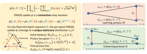
Figure 1: The overview of our stochastic gradient Langevin unlearning framework. (Left) Given a mini-batch sequence $\mathcal{B}$, the learning process $\mathcal{M}$ induces a regular polyhedron where each vertex corresponds to a stationary distribution $\nu_{\mathcal{D}|\mathcal{B}}$ for each dataset $\mathcal{D}$. $\nu_{\mathcal{D}|\mathcal{B}}$ and $\nu_{\mathcal{D|\mathcal{B}}^{\prime}}$ are adjacent if $\mathcal{D},\mathcal{D}^{\prime}$ differ in one data point. There is an uniform upper bound $Z_{\mathcal{B}}$ for the infinite Wasserstein distance $W_{\infty}$ between any pair of adjacent distributions $\nu_{\mathcal{D}|\mathcal{B}}$ and $\nu_{\mathcal{D|\mathcal{B}}^{\prime}}$. Intuitively, smaller $Z_{\mathcal{B}}$ implies an “simpler” unlearning problem, since transporting from $\nu_{\mathcal{D}|\mathcal{B}}$ to $\nu_{\mathcal{D|\mathcal{B}}^{\prime}}$ is easier. (Right) Learning and unlearning processes on adjacent datasets. We apply PABI analysis to convert the initial $W_{\infty}$ bound to Rényi difference bound $d_{\alpha}^{\mathcal{B}}$, and apply joint convexity of KL divergence to obtain the final privacy loss $\varepsilon$, which also take the randomness of $\mathcal{B}$ into account.

1.1 Our Contributions

We propose stochastic gradient Langevin unlearning, an approximate unlearning framework based on projected noisy stochastic gradient descent (PNSGD). To the best of our knowledge, we are the first to provide a thorough analysis of mini-batch gradient methods for approximate unlearning problems. Mini-batch private learning algorithms, such as DP-SGD (Abadi et al., 2016), have achieved great success due to their scalability compared to their full-batch counterparts. Prior works (Neel et al., 2021; Chien et al., 2024) focus on full-batch gradient algorithms while the benefit of the mini-batch gradient is still unclear for approximate unlearning problems. Our results show that PNSGD can be well applied to approximate unlearning problems with a substantial improvement in privacy-utility-complexity trade-offs for practical usage. Moreover, our stochastic gradient Langevin unlearning framework brings various benefits, including (1) provable computational benefit compared to retraining from scratch and (2) naturally supporting sequential and batch unlearning for multiple data point removal.

The core idea of our stochastic gradient Langevin unlearning is illustrated in Figure 1. Given a training dataset $\mathcal{D}$ and a fixed mini-batch sequence $\mathcal{B}$, we learn the model parameter with PNSGD. For sufficient learning epochs, we prove that the law of the PNSGD learning process converges to an unique stationary distribution $\nu_{\mathcal{D}|\mathcal{B}}$ (Theorem 3.1). When an unlearning request arrives, we update $\mathcal{D}$ to an adjacent dataset $\mathcal{D}^{\prime}$ so that the data point subject to such request is removed. The approximate unlearning problem can then be viewed as moving from the current distribution $\nu_{\mathcal{D}|\mathcal{B}}$ to the target distribution $\nu_{\mathcal{D}^{\prime}|\mathcal{B}}$ until $\varepsilon$-close in Rényi divergence for the desired privacy loss $\varepsilon$. Intuitively, if the starting distribution $\nu_{\mathcal{D}|\mathcal{B}}$ and the target distribution $\nu_{\mathcal{D}^{\prime}|\mathcal{B}}$ are “close”, we require less unlearning epochs to achieve a desired $\varepsilon$.

We prove this intuition formally in Theorem 3.2. We leverage the Privacy Amplification By Iteration (PABI) analysis (Feldman et al., 2018; Altschuler & Talwar, 2022a, b), which allows us to convert an initial infinite Wasserstein ($W_{\infty}$) distance to a Rényi divergence bound. We show that $K$ unlearning epochs lead to an exponentially fast decay in privacy loss from the initial $W_{\infty}$ distance bound $Z_{\mathcal{B}}$ of any pair of adjacent stationary distributions $\nu_{\mathcal{D}|\mathcal{B}},\nu_{\mathcal{D|\mathcal{B}}^{\prime}}$ under the strong convexity assumption. We later generalize it to the convex-only case (Corollary 3.10). More specifically, we show that $K$ unlearning epochs lead to privacy loss $\varepsilon=O(Z_{\mathcal{B}}^{2}c^{2Kn/b})$ for mini-batch size $b$, where we also characterize $Z_{\mathcal{B}}$ by tracking the $W_{\infty}$ distance of any two learning processes on adjacent datasets $\mathcal{D}$ and $\mathcal{D}^{\prime}$. To the best of our knowledge, we are the first to introduce PABI analysis for unlearning problems and achieve approximate unlearning guarantees for PNSGD. To prevent the worst-case bound induced by the fixed mini-batch sequence $\mathcal{B}$, we further utilize the randomness in the selection of $\mathcal{B}$ for an improved privacy bound (Corollary 3.9). Our approach naturally extends to multiple unlearning requests, including sequential and batch unlearning settings, which can be done by extending our analysis of tracking the $W_{\infty}$ distance bound $Z_{\mathcal{B}}$ for these cases (Theorem 3.11 and Corollary 3.12).

Our results demonstrate that smaller batch size $b$ leads to a better privacy loss decaying rate due to the more updates per epoch. Intuitively, more unlearning updates imply closer to the “retraining distribution” $\nu_{\mathcal{D}^{\prime}|\mathcal{B}}$ and thus better privacy. It highlights the benefit of the mini-batch setting for unlearning compared to prior works that only focus on full-batch gradient methods. Nevertheless, an extremely small $b$ can degrade the model utility and incur instability in practice, as the stationary distribution $\nu_{\mathcal{D}|\mathcal{B}}$ also depends on the design of mini-batches $\mathcal{B}$. Our results highlight a unique privacy-utility-complexity trade-off with respect to the mini-batch size $b$ for approximate unlearning.

Regarding the computational benefit compared to retraining from scratch, we may show epoch saving by comparing two $W_{\infty}$ distances, the one between initialization $\nu_{0}$ and $\nu_{\mathcal{D}^{\prime}|\mathcal{B}}$, which is $\Omega(1)$ in the worst case versus the other one between the adjacent distributions $\nu_{\mathcal{D}|\mathcal{B}}$ and $\nu_{\mathcal{D}^{\prime}|\mathcal{B}}$, which is upper bounded by $Z_{\mathcal{B}}\approx O(\eta M/b)$ for bounded gradient norm $M$ and step size $\eta$. For moderate mini-batch size $b$, our unlearning approach is more efficient than retraining from scratch. Even if one chooses $b=1$ (which leads to worse utility as mentioned earlier), our approach can still be more efficient as long as $\eta M$ is properly controlled. Our experiment shows that commonly used mini-batch size ($b\geq 32$) already leads to significant computational savings compared to retraining.

To examine the trade-off between privacy-utility-complexity of stochastic gradient Langevin unlearning, we conduct experiments through logistic regression tasks on benchmark datasets following a similar setting of Guo et al. (2020). We compared with the state-of-the-art gradient-based approximate unlearning solutions (Neel et al., 2021; Chien et al., 2024), albeit they only focus on full-batch setting $b=n$. Our analysis provides a significantly better privacy-utility-complexity trade-off even when we restrict ourselves to $b=n$, and further improves the results by adopting mini-batches. Under the same privacy constraint, stochastic gradient Langevin unlearning achieves similar utility while merely requiring $10\%,2\%$ of gradient computations compared to baselines for full and mini-batch settings respectively. It demonstrates the benefit of using mini-batches for approximate unlearning.

1.2 Related Works

Machine unlearning with privacy guarantees. The concept of approximate unlearning uses a probabilistic definition of $(\epsilon,\delta)$-unlearning motivated by differential privacy (Dwork et al., 2006), which is studied by Guo et al. (2020); Sekhari et al. (2021); Chien et al. (2022). Notably, the unlearning approach of these works involved Hessian inverse computation which can be computationally prohibitive in practice for high dimensional problems. Ullah et al. (2021) focus on exact unlearning via a sophisticated version of noisy SGD. Their analysis is based on total variation stability which is not directly applicable to approximate unlearning settings and different from our analysis focusing on Rényi divergence.  Neel et al. (2021) leverage full-batch PGD for (un)learning and achieve approximate unlearning by publishing the final parameters with additive Gaussian noise.  Gupta et al. (2021); Ullah & Arora (2023); Chourasia & Shah (2023) study the setting of adaptive unlearning requests, where the unlearning request may depend on the previous (un)learning results. It is possible to show that our framework is also capable of this adaptive setting since we do not keep any non-private internal states, albeit we only focus on non-adaptive settings in this work. We left a rigorous discussion for this as future work.

Comparison to Chien et al. (2024). Very recently, Chien et al. (2024) propose to leverage PNGD for learning and unlearning, where they establish approximate unlearning guarantees based on Langevin dynamic analaysis (Vempala & Wibisono, 2019) and track the Log-Sobolev conditions along the (un)learning processes (Gross, 1975; Chewi, Sinho, 2023). In contrast, we focus on the mini-batch setting (PNSGD), where our analysis is based on PABI and we track the $W_{\infty}$ distance along the (un)learning processes. There are pros and cons to these two types of analyses. On one hand, our results based on PABI analysis provide a better privacy-utility-complexity trade-off for sequential unlearning under a strongly convex setting. More specifically, we leverage standard triangle inequality for analyzing $W_{\infty}$ distance while Chien et al. (2024) require to adopt weak triangle inequality of Rényi divergence for each sequential unlearning request. This results in a worse estimation of sequential unlearning. On the other hand, Langevin dynamic analysis gives a unified analysis for non-convex settings where the convexity assumption of PABI analysis cannot be dropped (Altschuler & Talwar, 2022a, b). It is interesting to further explore the limit of these two analyses for unlearning problems, which we left as future work.

2 Preliminaries

We consider the empirical risk minimization (ERM) problem. Let $\mathcal{D}=\{\mathbf{d}_{i}\}_{i=1}^{n}$ be a training dataset with $n$ data point $\mathbf{d}_{i}$ taken from the universe $\mathcal{X}$. Let $f_{\mathcal{D}}(x)=\frac{1}{n}\sum_{i=1}^{n}f(x;\mathbf{d}_{i})$ be the objective function that we aim to minimize with learnable parameter $x\in\mathcal{C}_{R}$, where $\mathcal{C}_{R}=\{x\in\mathbb{R}^{d}\;|\;\|x\|\leq R\}$ is a closed ball of radius $R$. We denote $\Pi_{\mathcal{C}_{R}}:\mathbb{R}^{d}\mapsto\mathcal{C}_{R}$ to be an orthogonal projection to $\mathcal{C}_{R}$. The norm $\|\cdot\|$ is standard Euclidean $\ell_{2}$ norm. $\mathcal{P}(\mathcal{C})$ is denoted as the set of all probability measures over a closed convex set $\mathcal{C}$. Standard definitions such as convexity can be found in Appendix B. Finally, we use $x\sim\nu$ to denote that a random variable $x$ follows the probability distribution $\nu$. We say two datasets $\mathcal{D}$ and $\mathcal{D}^{\prime}$ are adjacent if they “differ” in only one data point. More specifically, we can obtain $\mathcal{D}^{\prime}$ from $\mathcal{D}$ by replacing one data point. We next introduce a useful idea which we termed Rényi difference.

Definition 2.1 (Rényi difference).

Let $\alpha>1$. For a pair of probability measures $\nu,\nu^{\prime}$ with the same support, the $\alpha$ Rényi difference $d_{\alpha}(\nu,\nu^{\prime})$ is defined as $d_{\alpha}(\nu,\nu^{\prime})=\max\left(D_{\alpha}(\nu||\nu^{\prime}),D_{\alpha}(\nu^{\prime}||\nu)\right),$ where $D_{\alpha}(\nu||\nu^{\prime})$ is the $\alpha$ Rényi divergence defined as $D_{\alpha}(\nu||\nu^{\prime})=\frac{1}{\alpha-1}\log\left(\mathbb{E}_{x\sim\nu^{\prime}}(\frac{\nu(x)}{\nu^{\prime}(x)})^{\alpha}\right).$

We are ready to introduce the formal definition of differential privacy and unlearning.

Definition 2.2 (Rényi Differential Privacy (RDP) (Mironov, 2017)).

Let $\alpha>1$. A randomized algorithm $\mathcal{M}:\mathcal{X}^{n}\mapsto\mathbb{R}^{d}$ satisfies $(\alpha,\varepsilon)$-RDP if for any adjacent dataset pair $\mathcal{D},\mathcal{D}^{\prime}\in\mathcal{X}^{n}$, the $\alpha$ Rényi difference $d_{\alpha}(\nu,\nu^{\prime})\leq\varepsilon$, where $\mathcal{M}(\mathcal{D})\sim\nu$ and $\mathcal{M}(\mathcal{D}^{\prime})~{}\sim\nu^{\prime}$.

It is known to the literature that an $(\alpha,\varepsilon)$-RDP guarantee can be converted to the popular $(\epsilon,\delta)$-DP guarantee (Dwork et al., 2006) relatively tight (Mironov, 2017). As a result, we will focus on establishing results with respect to $\alpha$ Rényi difference (and equivalently $\alpha$ Rényi difference). Next, we introduce our formal definition of unlearning based on $\alpha$ Rényi difference as well.

Definition 2.3 (Rényi Unlearning (RU)).

Consider a randomized learning algorithm $\mathcal{M}:\mathcal{X}^{n}\mapsto\mathbb{R}^{d}$ and a randomized unlearning algorithm $\mathcal{U}:\mathcal{R}^{d}\times\mathcal{X}^{n}\times\mathcal{X}^{n}\mapsto\mathcal{R}^{d}$. We say $(\mathcal{M},\mathcal{U})$ achieves $(\alpha,\varepsilon)$-RU if for any $\alpha>1$ and any adjacent datasets $\mathcal{D},\mathcal{D}^{\prime}$, the $\alpha$ Rényi difference $d_{\alpha}(\rho,\nu^{\prime})\leq\varepsilon,$ where $\mathcal{U}(\mathcal{M}(\mathcal{D}),\mathcal{D},\mathcal{D}^{\prime})\sim\rho$ and $\mathcal{M}(\mathcal{D}^{\prime})\sim\nu^{\prime}$.

Our Definition 2.3 can be converted to the standard $(\epsilon,\delta)$-unlearning definition defined in Guo et al. (2020); Sekhari et al. (2021); Neel et al. (2021), similar to RDP to DP conversion (see Appendix K). Since we work with the replacement definition of dataset adjacency, to unlearn a data point $\mathbf{d}_{i}$ we can simply replace it with any data point $\mathbf{d}_{i}^{\prime}\in\mathcal{X}$ for the updated dataset $\mathcal{D}^{\prime}$ in practice. One may also repeat the entire analysis with the objective function being the summation of individual loss for the standard add/remove notion of dataset adjacency. Finally, we will also leverage the infinite Wasserstein distance in our analysis.

Definition 2.4 ($W_{\infty}$ distance).

The $\infty$-Wasserstein distance between distributions $\mu$ and $\nu$ on a Banach space $(\mathbb{R}^{d},\|\cdot\|)$ is defined as $W_{\infty}(\mu,\nu)=\inf_{\gamma\in\Gamma(\mu,\nu)}\operatorname*{ess\,sup}_{(x,y)\sim\gamma}\|x-y\|,$ where $(x,y)\sim\gamma$ means that the essential supremum is taken relative to measure $\gamma$ over $\mathbb{R}^{d}\times\mathbb{R}^{d}$ parametrized by $(x,y)$. $\Gamma(\mu,\nu)$ is the collection of couplings of $\mu$ and $\nu$.

Algorithm 1 Stochastic gradient Langevin unlearning

1:  Minibatch Generation: randomly partition indices $[n]$ into $n/b$ mini-batches of size $b$: $\mathcal{B}^{0},\ldots,\mathcal{B}^{n/b-1}$.

2:  Learning process $\mathcal{M}(\mathcal{D})$: given a dataset $\mathcal{D}=\{\mathbf{d}_{i}\}_{i=1}^{n}\in\mathcal{X}^{n}$, sample initial parameter $x_{0}^{0}$ from a given initialization distribution $\nu_{0}$ supported on $\mathcal{C}_{R}$.

3:  for  epoch $t=0,\ldots,T-1$ do

4:     for  iteration $j=0,\ldots,n/b-1$ do

5:        $x^{j+1}_{t}=\Pi_{\mathcal{C}_{R}}\left(x^{j}_{t}-\eta g(x^{j}_{t},\mathcal{B}^{j})+\sqrt{2\eta\sigma^{2}}W^{j}_{t}\right),$ where $g(x^{j}_{t},\mathcal{B}^{j})=\frac{1}{b}\sum_{i\in\mathcal{B}^{j}}\nabla f(x^{j}_{t};\mathbf{d}_{i})$ and $W^{j}_{t}\stackrel{{\scriptstyle\text{iid}}}{{\sim}}\mathcal{N}(0,I_{d})$.

6:     end for

7:     $x^{0}_{t+1}=x^{n/b}_{t}$

8:  end for

9:  Unlearning process $\mathcal{U}(\mathcal{M}(\mathcal{D}),\mathcal{D}^{\prime})$: given an updated dataset $\mathcal{D}^{\prime}=\{\mathbf{d}_{i}^{\prime}\}_{i=1}^{n}\in\mathcal{X}^{n}$ and current parameter $y_{0}^{0}$,

10:  for  epoch $k=0,\ldots,K-1$ do

11:     for  iteration $j=0,\ldots,n/b-1$ do

12:        $y^{j+1}_{k}=\Pi_{\mathcal{C}_{R}}\left(y^{j}_{k}-\eta g(y^{j}_{k},\mathcal{B}^{j})+\sqrt{2\eta\sigma^{2}}W^{j}_{k}\right),$ where $g(y^{j}_{k},\mathcal{B}^{j})=\frac{1}{b}\sum_{i\in\mathcal{B}^{j}}\nabla f(y^{j}_{k};\mathbf{d}_{i}^{\prime})$ and $W^{j}_{k}\stackrel{{\scriptstyle\text{iid}}}{{\sim}}\mathcal{N}(0,I_{d})$.

13:     end for

14:     $y^{0}_{k+1}=y^{n/b}_{k}$

15:  end for

3 Stochactic Gradient Langevin Unlearning

We now introduce our stochastic gradient Langevin unlearning strategy. We propose to leverage the projected noisy SGD (PNSGD) with a cyclic mini-batch strategy. Note that this mini-batch strategy is not only commonly used for practical DP-SGD implementations in privacy libraries (Yousefpour et al., 2021), but also in theoretical analysis for DP guarantees (Ye & Shokri, 2022). For the learning algorithm $\mathcal{M}$, we propose to optimize the objective function with projected noisy SGD on dataset $\mathcal{D}$ (line 3-8 in Algorithm 1). $\eta,\sigma^{2}>0$ are hyperparameters of step size and noise variance respectively. The initialization $\nu_{0}$ is an arbitrary distribution supported on $\mathcal{C}_{R}$ if not specified. For the unlearning algorithm $\mathcal{U}$, we fine-tune the current parameter on the updated dataset $\mathcal{D}^{\prime}$ subject to the unlearning request (line 10-15 in Algorithm 1) with $y_{0}^{0}=x_{T}^{0}=\mathcal{M}(\mathcal{D})$. For the rest of the paper, we denote $\nu_{t}^{j},\rho_{k}^{j}$ as the probability density of $x_{t}^{j},y_{k}^{j}$ respectively. Furthermore, we denote $\mathcal{B}=\{\mathcal{B}^{j}\}_{j=0}^{n/b-1}$ the minibatch sequence described in Algorithm 1, where $b$ is the step size and we assume $n$ is divided by $b$ throughout the paper for simplicity. We use $\nu_{\cdot|\mathcal{B}}$ to denote the conditional distribution of $\nu_{\cdot}$ given $\mathcal{B}$.

3.1 Limiting distribution and general idea

Now we introduce the general idea of our stochastic gradient Langevin unlearning, which is illustrated in Figure 1. We first prove that for any fixed mini-batch sequence $\mathcal{B}$, the limiting distribution $\nu_{\mathcal{D}|\mathcal{B}}$ of the learning process exists, is unique, and stationery.

Theorem 3.1.

Suppose that the closed convex set $\mathcal{C}_{R}\subset\mathbb{R}^{d}$ is bounded with $\mathcal{C}_{R}$ having a positive Lebesgue measure and that $\nabla f(\cdot;\mathbf{d}_{i}):\mathcal{C}_{R}\to\mathbb{R}^{d}$ is continuous for all $i\in[n]$. The Markov chain $\{x_{t}:=x_{t}^{0}\}$ in Algorithm 1 for any fixed mini-batch sequence $\mathcal{B}$ admits a unique invariant probability measure $\nu_{\mathcal{D}|\mathcal{B}}$ on the Borel $\sigma$-algebra of $\mathcal{C}_{R}$. Furthermore, for any $x\in\mathcal{C}_{R}$, the distribution of $x_{t}$ conditioned on $x_{0}=x$ converges weakly to $\nu_{\mathcal{D}|\mathcal{B}}$ as $t\to\infty$.

The proof of Theorem 3.1 is deferred to Appendix C and is based on applying the results in Meyn & Tweedie (2012) to establish the ergodicity of the learning process $x_{t}^{0}$.

3.2 Unlearning guarantees with PABI analysis

We prove the following unlearning guarantee for stochastic gradient Langevin unlearning described in Algorithm 1 for any fixed mini-batch sequence $\mathcal{B}$. We will later provide a slightly better bound by considering the randomness of $\mathcal{B}$.

Theorem 3.2 (RU guarantee of PNSGD unlearning, fixed $\mathcal{B}$).

Assume $\forall\mathbf{d}\in\mathcal{X}$, $f(x;\mathbf{d})$ is $L$-smooth, $M$-Lipchitz and $m$-strongly convex in $x$. Let the learning and unlearning processes follow Algorithm 1 with $y_{0}^{0}=x_{T}^{0}=\mathcal{M}(\mathcal{D})$. Given any fixed mini-batch sequence $\mathcal{B}$, for any $\alpha>1$, let $\eta\leq\frac{1}{L}$, the output of the $K^{th}$ unlearning iteration satisfies $(\alpha,\varepsilon)$-RU with $c=1-\eta m$, where

$$\varepsilon\leq\frac{\alpha-1/2}{\alpha-1}\left(\varepsilon_{1}(2\alpha)+\varepsilon_{2}(2\alpha)\right),$$

$$\varepsilon_{1}(\alpha)=\frac{\alpha(2R)^{2}}{2\eta\sigma^{2}}c^{2Tn/b},\;\varepsilon_{2}(\alpha)=\frac{\alpha Z_{\mathcal{B}}^{2}}{2\eta\sigma^{2}}c^{2Kn/b},$$

$$Z_{\mathcal{B}}=2Rc^{Tn/b}+\min\left(\frac{1-c^{Tn/b}}{1-c^{n/b}}\frac{2\eta M}{b},2R\right).$$

Our proof is based on the Privacy Amplification By Iteration (PABI) (Feldman et al., 2018), which has also been leveraged for providing the DP guarantee and mixing time of PNSGD by Altschuler & Talwar (2022a, b). To understand the main idea of the proof, we first introduce the notion of contractive noisy iteration.

Definition 3.3 (Contractive Noisy Iteration ($c$-CNI)).

Given an initial distribution $\mu_{0}\in\mathcal{P}(\mathbb{R}^{d})$, a sequence of (random) $c$-contractive (equivalently, $c$-Lipschitz) functions $\psi_{k}:\mathbb{R}^{d}\mapsto\mathbb{R}^{d}$, and a sequence of noise distributions $\zeta_{k}$, we define the $c$-Contractive Noisy Iteration ($c$-CNI) by the update rule $X_{k+1}=\psi_{k+1}(X_{k})+W_{k+1},$ where $W_{k+1}\sim\zeta_{k}$ independently and $X_{0}\sim\mu_{0}$. We denote the law of the final iterate $X_{K}$ by $\text{CNI}_{c}(\mu_{0},\{\psi_{k}\},\{\zeta_{k}\})$.

Feldman et al. (2018) provide the following metric-aware bound of the Rényi divergence between two $c$-CNI processes, which is simplified by Altschuler & Talwar (2022b).

Lemma 3.4 (Metric-aware PABI bound (Feldman et al., 2018), simplified by Altschuler & Talwar (2022b) in Proposition 2.10).

Suppose $X_{K}\sim\text{CNI}_{c}(\mu_{0},\{\psi_{k}\},\{\zeta_{k}\})$ and $X_{K}^{\prime}\sim\text{CNI}_{c}(\mu_{0}^{\prime},\{\psi_{k}\},\{\zeta_{k}\})$ where the initial distribution satisfy $W_{\infty}(\mu_{0},\mu_{0}^{\prime})\leq Z$, the update function $\psi_{k}$ are $c$-contractive, and the noise distributions $\zeta_{k}=\mathcal{N}(0,\sigma^{2}I_{d})$. Then we have

$$D_{\alpha}(X_{K}||X_{K}^{\prime})\leq\frac{\alpha Z^{2}}{2\sigma^{2}}\begin{cases}c^{2K}&\text{if }c<1\\ 1/K&\text{if }c=1\end{cases}.$$ (1)

In light of Lemma 3.4, if we can characterize the initial $W_{\infty}$ distance, the Rényi divergence between two $c$-CNI processes can be bounded. Note that the PNSGD update is indeed a $c$-CNI with $c<1$ under strong convexity assumption. We further provide the following two lemmas to track the $W_{\infty}$ distance along the learning process.

Lemma 3.5 ($W_{\infty}$ between adjacent PNSGD learning processes).

Consider the learning process in Algorithm 1 on adjacent datasets $\mathcal{D}$ and $\mathcal{D}^{\prime}$ and a fixed mini-batch sequence $\mathcal{B}$. Assume $\forall\mathbf{d}\in\mathcal{X}$, $f(x;\mathbf{d})$ is $L$-smooth, $M$-Lipschitz and $m$-strongly convex in $x$. Let the index of different data point between $\mathcal{D},\mathcal{D}^{\prime}$ belongs to mini-batch $\mathcal{B}^{j_{0}}$. Then for $\eta\leq\frac{1}{L}$ and let $c=(1-\eta m)$, we have

$$W_{\infty}(\nu_{T|\mathcal{B}}^{0},\nu_{T|\mathcal{B}}^{0,\prime})\leq\min\left(\frac{1-c^{Tn/b}}{1-c^{n/b}}c^{n/b-j_{0}-1}\frac{2\eta M}{b},2R\right).$$

Lemma 3.6 ($W_{\infty}$ between PNSGD learning process to its stationary distribution).

Following the same setting as in Theorem 3.2 and denote the initial distribution of the unlearning process as $\nu_{0}^{0}$. Then we have

$$W_{\infty}(\nu_{T|\mathcal{B}}^{0},\nu_{\mathcal{D}|\mathcal{B}})\leq(1-\eta m)^{Tn/b}W_{\infty}(\nu_{0}^{0},\nu_{\mathcal{D}|\mathcal{B}}).$$

We are ready to provide the sketch of proof for Theorem 3.2.

Sketch of proof. First note that the PNSGD update leads to a $(1-\eta m)$-CNI process when $\eta\leq 1/L$ for any mini-batch sequence. Recall that $y_{k}^{j}$ is the unlearning process at epoch $k$ at iteration $j$, starting from $y_{0}^{0}=x_{T}^{0}=\mathcal{M}(\mathcal{D})$. Consider the “adjacent” process $y_{k}^{j,\prime}$ starting from $y_{0}^{0,\prime}=x_{T}^{0,\prime}=\mathcal{M}(\mathcal{D}^{\prime})$ but still fine-tune on $\mathcal{D}^{\prime}$ so that $y_{k}^{j},y_{k}^{j,\prime}$ only differ in their initialization. Now, consider three distributions: $\nu_{\mathcal{D}|\mathcal{B}},\nu_{T|\mathcal{B}}^{0},\rho_{K|\mathcal{B}}^{0}$ are the stationary distribution for the learning processes, learning process at epoch $T$ and unlearning process at epoch $K$ respectively. Similarly, consider the “adjacent” processes that learn on $\mathcal{D}^{\prime}$ and still unlearn on $\mathcal{D}^{\prime}$ (see Figure 1 for the illustration). Denote distributions $\nu_{\mathcal{D}^{\prime}|\mathcal{B}},\nu_{T|\mathcal{B}}^{0,\prime},\rho_{K|\mathcal{B}}^{0,\prime}$ for these processes similarly. Note that our goal is to bound $d_{\alpha}(\rho_{K|\mathcal{B}}^{0},\nu_{T|\mathcal{B}}^{0,\prime})$ for the RU guarantee. By weak triangle inequality (Mironov, 2017), we can upper bound it in terms of $d_{2\alpha}(\rho_{K|\mathcal{B}}^{0},\nu_{\mathcal{D}^{\prime}|\mathcal{B}})$ and $d_{2\alpha}(\nu_{\mathcal{D}^{\prime}|\mathcal{B}},\nu_{T|\mathcal{B}}^{0,\prime})$, which are the $\varepsilon_{2}$ and $\varepsilon_{1}$ terms in Theorem 3.2 respectively. For $d_{\alpha}(\nu_{\mathcal{D}^{\prime}|\mathcal{B}},\nu_{T|\mathcal{B}}^{0,\prime})$, we leverage the naive $2R$ bound for the $W_{\infty}$ distance between $\nu_{\mathcal{D}^{\prime}|\mathcal{B}},\nu_{0|\mathcal{B}}^{0,\prime}$ and applying Lemma 3.4 leads to the desired result. For $d_{\alpha}(\rho_{K|\mathcal{B}}^{0},\nu_{\mathcal{D}^{\prime}|\mathcal{B}})$, by triangle inequality of $W_{\infty}$ and Lemma 3.5, 3.6 one can show that the $W_{\infty}$ between $\rho_{0|\mathcal{B}}^{0},\nu_{\mathcal{D}^{\prime}|\mathcal{B}}$ is bounded by $Z_{\mathcal{B}}$ in Theorem 3.2. Further applying Lemma 3.4 again completes the proof.

Remark 3.7.

Our proof only relies on the bounded gradient difference $\|\nabla f(x;\mathbf{d})-\nabla f(x;\mathbf{d}^{\prime})\|\leq 2M$ $\forall x\in\mathbb{R}^{d}$ and $\forall\mathbf{d},\mathbf{d}^{\prime}\in\mathcal{X}$ hence $M$-Lipchitz assumption can be replaced. In practice, we can leverage the gradient clipping along with a $\ell_{2}$ regularization for the convex objective function.

The convergent case. In practice, one often requires the training epoch $T$ to be sufficiently large so that the model is “well-trained”, where a similar assumption is made in the prior unlearning literature (Guo et al., 2020; Sekhari et al., 2021). Under this assumption, we can further simplify Theorem 3.2 into the following corollary.

Corollary 3.8.

Under the same setting as of Theorem 3.2. When we additionally assume $T$ is sufficiently large so that $y_{0}^{0}=M(\mathcal{D})\sim\nu_{\mathcal{D}|\mathcal{B}}$. Then for any $\alpha>1$ and $\eta\leq\frac{1}{L}$, the output of the $K^{th}$ unlearning iteration satisfies $(\alpha,\varepsilon)$-RU with $c=1-\eta m$, where

$$\varepsilon\leq\frac{\alpha Z_{\mathcal{B}}^{2}}{2\eta\sigma^{2}}c^{2Kn/b},Z_{\mathcal{B}}=\min\left(\frac{1}{1-c^{n/b}}\frac{2\eta M}{b},2R\right).$$

For simplicity, the rest of the discussion on our stochastic gradient Langevin unlearning will based on the training convergent assumption.

From Corollary 3.8 one can observe that a smaller $b$ leads to a better decaying rate ($c^{2Kn/b}$) but also a potentially worse initial distance $Z_{\mathcal{B}}=O(1/((1-c^{n/b})b))$. In general, choosing a smaller $b$ still leads to less epoch for achieving the desired privacy loss. In practice, choosing $b$ too small (e.g., $b=1$) can not only degrade the utility but also incur instability (i.e., large variance) of the convergent distribution $\nu_{\mathcal{D}|\mathcal{B}}$, as $\nu_{\mathcal{D}|\mathcal{B}}$ depends on the design of mini-batches $\mathcal{B}$. One should choose a moderate $b$ to balance between privacy and utility, which is the unique privacy-utility-complexity trade-off with respect to $b$ revealed by our analysis.

Computational benefit compared to retraining. In the view of Corollary 3.8 or Lemma 3.4, it is not hard to see that a smaller initial $W_{\infty}$ distance leads to fewer PNSGD (un)learning epochs for being $\varepsilon$-close to a target distribution $\nu_{\mathcal{D}^{\prime}|\mathcal{B}}$ in terms of Rényi difference $d_{\alpha}$. For stochastic gradient Langevin unlearning, we have provided a uniform upper bound $Z_{\mathcal{B}}=O(\eta M/((1-c^{n/b})b))$ of such initial $W_{\infty}$ distance in Lemma 3.5. On the other hand, even if both $\nu_{0},\nu_{\mathcal{D}}$ are both Gaussian with identical various and mean difference norm of $\Omega(1)$, we have $W_{\infty}(\nu_{0},\nu_{\mathcal{D}^{\prime}|\mathcal{B}})=\Omega(1)$ for retraining from scratch. Our results show that a larger mini-batch size $b$ leads to more significant complexity savings compared to retraining. As we discussed above, one should choose a moderate size $b$ to balance between privacy and utility. In our experiment, we show that for commonly used mini-batch sizes (i.e., $b\geq 32$), our stochastic gradient Langevin unlearning is still much more efficient in complexity compared to retraining.

Improved bound with randomized $\mathcal{B}$. So far our results are based on a fixed (worst-case) mini-batch sequence $\mathcal{B}$. One can improve the privacy bound in Corollary 3.8 by taking the randomness of $\mathcal{B}$ into account under a non-adaptive unlearning setting. That is, the unlearning request is independent of the mini-batch sequence $\mathcal{B}$. See also our discussion in the related work. We leverage Lemma 4.1 in Ye & Shokri (2022), which is an application of joint convexity of KL divergence. By combining with Corollary 3.8, we arrive at the following improved bound.

Corollary 3.9.

Under the same setting as of Theorem 3.2 but with random mini-batch sequences described in Algorithm 1. Then for any $\alpha>1$, and $\eta\leq\frac{1}{L}$, the output of the $K^{th}$ unlearning iteration satisfies $(\alpha,\varepsilon)$-RU with $c=1-\eta m$, where

$$\varepsilon\leq\frac{1}{\alpha-1}\log\left(\mathbb{E}_{\mathcal{B}}\exp\left(\frac{\alpha(\alpha-1)Z_{\mathcal{B}}^{2}}{2\eta\sigma^{2}}c^{2Kn/b}\right)\right),$$

where $Z_{\mathcal{B}}$ is the bound described in Lemma 3.5.

It slightly improves the privacy bound of Corollary 3.8 by the average case of $\mathcal{B}$ instead of the worst case.

Different mini-batch sampling strategies. We remark that our analysis can be extended to other mini-batch sampling strategies, such as sampling without replacement for each iteration. However, this strategy leads to a worse $Z_{\mathcal{B}}$ in our analysis of Lemma 3.5, which may seem counter-intuitive at first glance. This is due to the nature of the essential supremum taken in $W_{\infty}$. Although sampling without replacement leads to a smaller probability of sampling the index that gets modified due to the unlearning request, it is still non-zero for each iteration. Thus the worst-case difference $2\eta M/b$ between two adjacent learning processes in the mini-batch gradient update occurs at each iteration, which degrades the factor $1/(1-c^{n/b})$ to $1/(1-c)$ in Lemma 3.5. As a result, we choose to adopt the cyclic mini-batch strategy so that such a difference is guaranteed to occur only once per epoch and thus a better bound on $W_{\infty}$.

Without strong convexity. Since Lemma 3.4 also applies to the convex-only case (i.e., $m=0$ so that $c=1$), repeating the same analysis leads to the following extension.

Corollary 3.10.

Under the same setting as of Theorem 3.2 but without strong convexity (i.e., $m=0$). When we additionally assume $T$ is sufficiently large so that $y_{0}^{0}=M(\mathcal{D})\sim\nu_{\mathcal{D}|\mathcal{B}}$. Then for any $\alpha>1$, and $\eta\leq\frac{1}{L}$, the output of the $K^{th}$ unlearning iteration satisfies $(\alpha,\varepsilon)$-RU, where

$$\varepsilon\leq\frac{\alpha Z_{\mathcal{B}}^{2}}{2\eta\sigma^{2}}\frac{b}{Kn},Z_{\mathcal{B}}=\min\left(\frac{2\eta MT}{b},2R\right).$$

There are several remarks for Corollary 3.10. First, the privacy loss now only decays linearly instead of exponentially as opposed to the strongly convex case. Second, $Z_{\mathcal{B}}$ now can grow linearly in training epoch $T$. As a result, the computational benefit of our approach compared to retraining may vanish in this scenario. We conjecture a better analysis is needed beyond strong convexity.

3.3 Unlearning Multiple Data Points

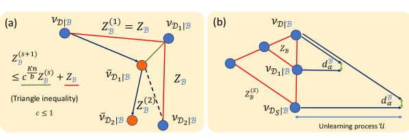
Figure 2: Illustration of (a) sequential unlearning and (b) batch unlearning. In both cases, the key idea is to establish an upper bound on the initial $W_{\infty}$ distance. (a) For sequential unlearning, the initial $W_{\infty}$ distance bound $Z_{\mathcal{B}}^{(s)}$ for each $s^{th}$ unlearning request can be derived with triangle inequality. (b) For batch unlearning, we analyze the case that two learning processes can differ in $S\geq 1$ points (Corollary 3.12).

So far we have focused on one unlearning request and unlearning one point. In practice, multiple unlearning requests can arrive sequentially (sequential unlearning) and each unlearning request may require unlearning multiple points (batch unlearning). Below we demonstrate that our stochastic gradient Langevin unlearning naturally supports sequential and batch unlearning as well.

Sequential unlearning. As long as we can characterize the initial $W_{\infty}$ distance for any mini-batch sequences, we have the corresponding $(\alpha,\varepsilon)$-RU guarantee due to Corollary 3.8. Thanks to our geometric view of the unlearning problem (Figure 2) and $W_{\infty}$ is indeed a metric, applying triangle inequality naturally leads to an upper bound on the initial $W_{\infty}$ distance. By combining Lemma 3.5 and Lemma 3.6, we have the following sequential unlearning guarantee.

Theorem 3.11 ($W_{\infty}$ bound for sequential unlearning).

Under the same assumptions as in Corollary 3.8. Assume the unlearning requests arrive sequentially such that our dataset changes from $\mathcal{D}=\mathcal{D}_{0}\rightarrow\mathcal{D}_{1}\rightarrow\ldots\rightarrow\mathcal{D}_{S}$, where $\mathcal{D}_{s},\mathcal{D}_{s+1}$ are adjacent. Let $y_{k}^{j,(s)}$ be the unlearned parameters for the $s^{th}$ unlearning request at $k^{th}$ unlearning epoch and $j^{th}$ iteration following Algorithm (1) on $\mathcal{D}_{s}$ and $y_{0}^{0,(s+1)}=y_{K_{s}}^{0,(s)}\sim\bar{\nu}_{\mathcal{D}_{s}|\mathcal{B}}$, where $y_{0}^{0,(0)}=x_{\infty}$ and $K_{s}$ is the unlearning steps for the $s^{th}$ unlearning request. For any $s\in[S]$, we have $W_{\infty}(\bar{\nu}_{\mathcal{D}_{s-1}|\mathcal{B}},\nu_{\mathcal{D}_{s}|\mathcal{B}})\leq Z_{\mathcal{B}}^{(s)},$ where $Z_{\mathcal{B}}^{(s+1)}=\min(c^{K_{s}n/b}Z_{\mathcal{B}}^{(s)}+Z_{\mathcal{B}},2R)$, $\;Z_{\mathcal{B}}^{(1)}=Z_{\mathcal{B}}$, $Z_{\mathcal{B}}$ is described in Corollary 3.8 and $\;c=1-\eta m$.

By combining Corollary 3.8 and Theorem 3.11, we can establish the least unlearning iterations of each unlearning request $\{K_{s}\}_{s=1}^{S}$ to achieve $(\alpha,\varepsilon)$-RU simultaneously. Notably, our sequential unlearning bound is much better than the one in Chien et al. (2024), especially when the number of unlearning requests is large. The key difference is that Chien et al. (2024) have to leverage weak triangle inequality for Rényi divergence, which double the Rényi divergence order $\alpha$ for each sequential unlearning request. In contrast, since our analysis only requires tracking the initial $W_{\infty}$ distance, where the standard triangle inequality can be applied. As a result, our analysis can better handle the sequential unlearning case. We also demonstrate in Section 4 that the benefit offered by our results is significant in practice.

Batch unlearning. We can extend Lemma 3.5 to the case that adjacent dataset $\mathcal{D},\mathcal{D}^{\prime}$ can differ in $S\geq 1$ points. This leads to the following corollary.

Corollary 3.12 ($W_{\infty}$ bound for batch unlearning).

Consider the learning process in Algorithm 1 on adjacent dataset $\mathcal{D}$ and $\mathcal{D}^{\prime}$ that differ in $1\leq S$ points and a fixed mini-batch sequence $\mathcal{B}$. Assume $\forall\mathbf{d}\in\mathcal{X}$, $f(x;\mathbf{d})$ is $L$-smooth, $M$-Lipschitz and $m$-strongly convex in $x$. Let the index of different data point between $\mathcal{D},\mathcal{D}^{\prime}$ belongs to mini-batches $\mathcal{B}^{j_{0}},\mathcal{B}^{j_{1}},\ldots,\mathcal{B}^{j_{G-1}}$, each of which contains $1\leq S_{j_{g}}\leq b$ such that $\sum_{g=0}^{G-1}S_{j_{g}}=S$. Then for $\eta\leq\frac{1}{L}$ and $c=(1-\eta m)$, we have

$$W_{\infty}(\nu_{T|\mathcal{B}}^{0},\nu_{T|\mathcal{B}}^{0,\prime})$$

$$\leq\min\left(\frac{1-c^{T}}{1-c}\sum_{g=0}^{G-1}c^{n/b-j_{g}-1}\frac{2\eta MS_{j_{g}}}{b},2R\right).$$

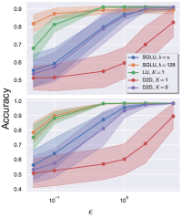
(a)

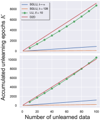
(b)

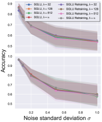
(c)

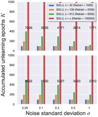
(d)

Figure 3: Main experiments, where the top and bottom rows are for MNIST and CIFAR10 respectively. (a) Compare to baseline for unlearning one point using limited $K$ unlearning epoch. For SGLU, we use only $K=1$ unlearning epoch. For D2D, we allow it to use $K=1,5$ unlearning epochs. (b) Unlearning $100$ points sequentially versus baseline. For LU, since their unlearning complexity only stays in a reasonable range when combined with batch unlearning of size $S$ sufficiently large, we report such a result only. (c,d) Noise-accuracy-complexity trade-off of SGLU for unlearning $100$ points sequentially with various mini-batch sizes $b$, where all methods achieve $(\epsilon,1/n)$-unlearning guarantee with $\epsilon=0.01$. We also report the required accumulated epochs for retraining for each $b$.

4 Experiments

Benchmark datasets. We consider binary logistic regression with $\ell_{2}$ regularization. We conduct experiments on MNIST (Deng, 2012) and CIFAR10 (Krizhevsky et al., 2009), which contain 11,982 and 10,000 training instances respectively. We follow the setting of (Guo et al., 2020; Chien et al., 2024) to distinguish digits $3$ and $8$ for MNIST so that the problem is a binary classification. For the CIFAR10 dataset, we distinguish labels $3$ (cat) and $8$ (ship) and leverage the last layer of the public ResNet18 (He et al., 2016) embedding as the data features, which follows the setting of Guo et al. (2020) with public feature extractor.

Baseline methods. Our baseline methods include Delete-to-Descent (D2D) (Neel et al., 2021) and Langevin Unlearning (LU) (Chien et al., 2024), which are the state-of-the-art full-batch gradient-based approximate unlearning methods. Note that when our Stochastic Gradient Langevin Unlearning (SGLU) chooses $b=n$ (i.e., full batch), the learning and unlearning iterations become PNGD which is identical to LU. Nevertheless, the corresponding privacy bound is still different as we leverage the analysis of PABI instead of those based on Langevin dynamics in Chien et al. (2024). Hence, we still treat these two methods differently in our experiment. For D2D, we leverage Theorem 9 and 28 in (Neel et al., 2021) for privacy accounting depending on whether we allow D2D to have an internal non-private state. Note that allowing an internal non-private state provides a weaker notion of privacy guarantee (Neel et al., 2021) and both SGLU and LU by default do not require it. We include those theorems for D2D and a detailed explanation of its possible non-privacy internal state in Appendix L. For LU, we leverage their Theorem 3.2, and 3.3 for privacy accounting (Chien et al., 2024), which are included in Appendix M.

All experimental details can be found in Appendix K, including how to convert $(\alpha,\varepsilon)$-RU to the standard $(\epsilon,\delta)$-unlearning guarantee. Throughout this section, we choose $\delta=1/n$ for each dataset and require all tested unlearning approaches to achieve $(\epsilon,\delta)$-unlearning with different $\epsilon$. We report test accuracy for all experiments as the utility metric. We set the learning iteration $T=10,20,50,1000$ to ensure SGLU converges for mini-batch size $b=32,128,512,n$ respectively. All results are averaged over $100$ independent trials with standard deviation reported as shades in figures.

Unlearning one data point with $K=1$ epoch. We first consider the setting of unlearning one data point using only one unlearning epoch (Figure 3a). For both LU and SGLU, we use only $K=1$ unlearning epoch. Since D2D cannot achieve a privacy guarantee with only limited (i.e., less than $10$) unlearning epoch without a non-private internal state, we allow D2D to have it and set $K=1,5$ in this experiment. Even in this case, SGLU still outperforms D2D in both utility and unlearning complexity. Compared to LU, our mini-batch setting either outperforms or is on par with it. Interestingly, we find that LU gives a better privacy bound compared to full-batch SGLU ($b=n$) and thus achieves better utility under the same privacy constraint, see Appendix M for the detailed comparisons of the privacy bounds. Nevertheless, due to the use of weak triangle inequality in LU analysis, we will see that our SGLU can outperform LU significantly for multiple unlearning requests.

Unlearning multiple data points. Let us consider the case of multiple ($100$) unlearning requests (Figure 3b). We let all methods achieve the same $(1,1/n)$-unlearning guarantee for a fair comparison. We do not allow D2D to have an internal non-private state anymore in this experiment for a fair comparison. Since the privacy bound of LU only gives reasonable unlearning complexity with a limited number of sequential unlearning updates (Chien et al., 2024), we allow it to unlearn $S=10$ points at once. We observe that SGLU requires roughly $10\%$ and $2\%$ of unlearning epochs compared to D2D and LU for $b=n$ and $b=128$ respectively, where all methods exhibit similar utility ($0.9$ and $0.98$ for MNIST and CIFAR10 respectively). It shows that SGLU is much more efficient compared to D2D and LU. Notably, while both SGLU with $b=n$ and LU (un)learn with PNGD iterations, the resulting privacy bound based on our PABI-based analysis is superior to the one pertaining to Langevin-dynamic-based analysis in Chien et al. (2024). See our discussion in Section 3.3 for the full details.

Privacy-utility-complexity trade-off. We now investigate the inherent utility-complexity trade-off regarding noise standard deviation $\sigma$ and mini-batch size $b$ for SGLU under the same privacy constraint, where we require all methods to achieve $(0.01,1/n)$-unlearning guarantee for $100$ sequential unlearning requests (Figure 3c and 3d). We can see that smaller $\sigma$ leads to a better utility, yet more unlearning epochs are needed for SGLU to achieve $\epsilon=0.01$. On the other hand, smaller mini-batch size $b$ requires fewer unlearning epochs $K$ as shown in Figure 3d, since more unlearning iterations are performed per epoch. Nevertheless, we remark that choosing $b$ too small may lead to degradation of model utility or instability. Decreasing the mini-batch size $b$ from $32$ to $1$ reduces the average accuracy of training from scratch from $0.87$ to $0.64$ and $0.97$ to $0.81$ on MNIST and CIFAR10 respectively for $\sigma=0.03$. In practice, one should choose a moderate mini-batch size $b$ to ensure both good model utility and unlearning complexity. Finally, we also note that SGLU achieves a similar utility while much better complexity compared to retraining from scratch, where SGLU requires at most $1,5$ unlearning epochs per unlearning request for $b=32,512$ respectively.

Appendix A Additional related works

Differential privacy of noisy gradient methods. DP-SGD (Abadi et al., 2016) is arguably the most popular method for ensuring a DP guarantee for machine learning models. Since it leverages the DP composition theorem and thus the privacy loss will diverge for infinite training epochs. Recently, researchers have found that if we only release the last step of the trained model, then we can do much better than applying the composition theorem. A pioneer work (Ganesh & Talwar, 2020) studied the DP properties of Langevin Monte Carlo methods. Yet, they do not propose to use noisy GD for general machine learning problems. A recent line of work (Ye & Shokri, 2022; Ryffel et al., 2022) shows that PNSGD training can not only provide DP guarantees, but also the privacy loss is at most a finite value even if we train with an infinite number of iterations. The main analysis therein is based on the analysis of Langevin Monte Carlo (Vempala & Wibisono, 2019; Chewi, Sinho, 2023). In the meanwhile, (Altschuler & Talwar, 2022a) also provided the DP guarantees for PNSGD training but with analysis based on PABI (Feldman et al., 2018). None of these works study how PNSGD can also be leveraged for machine unlearning.

Appendix B Standard definitions

Let $f:\mathbb{R}^{d}\mapsto\mathbb{R}$ be a mapping. We define smoothness, Lipschitzsness, and strong convexity as follows:

$$\text{$L$-smooth: }\forall~{}x,y\in\mathbb{R}^{d},\;\|\nabla f(x)-\nabla f(y)\|\leq L\|x-y\|$$ (2)

$$\text{$m$-strongly convex: }\forall~{}x,y\in\mathbb{R}^{d},\;\left\langle x-y,\nabla f(x)-\nabla f(y)\right\rangle\geq m\|x-y\|^{2}$$ (3)

$$\text{$M$-Lipschitzs: }\forall~{}x,y\in\mathbb{R}^{d},\;\|f(x)-f(y)\|\leq M\|x-y\|.$$ (4)

Furthermore, we say $f$ is convex means it is $0$-strongly convex.

Appendix C Existence of limiting distribution

Theorem.

Suppose that the closed convex set $\mathcal{C}_{R}\subset\mathbb{R}^{d}$ is bounded with $\mathcal{C}_{R}$ having a positive Lebesgue measure and that $\nabla f(\cdot;\mathbf{d}_{i}):\mathcal{C}_{R}\to\mathbb{R}^{d}$ is continuous for all $i\in[n]$. The Markov chain $\{x_{t}:=x_{t}^{0}\}$ in Algorithm 1 for any fixed mini-batch sequence $\mathcal{B}=\{\mathcal{B}^{j}\}_{j=1}^{n/b-1}$ admits a unique invariant probability measure $\nu_{\mathcal{D}|\mathcal{B}}$ on the Borel $\sigma$-algebra of $\mathcal{C}_{R}$. Furthermore, for any $x\in\mathcal{C}_{R}$, the distribution of $x_{t}$ conditioned on $x_{0}=x$ converges weakly to $\nu_{\mathcal{D}|\mathcal{B}}$ as $t\to\infty$.

The proof is almost identical to the proof of Theorem 3.1 in Chien et al. (2024) and we include it for completeness. We start by proving that the process $\{x_{t}:=x_{t}^{0}\}$ admits a unique invariant measure (Proposition C.1) and then show that the process converges to such measure which is in fact a probability measure (Theorem C.2). Combining these two results completes the proof of Theorem 3.1.

Proposition C.1.

Suppose that the closed convex set $\mathcal{C}_{R}\subset\mathbb{R}^{d}$ is bounded with $\textrm{Leb}(\mathcal{C}_{R})>0$ where Leb denotes the Lebesgue measure and that $\nabla f(\cdot;\mathbf{d}_{i}):\mathcal{C}_{R}\to\mathbb{R}^{d}$ is continuous for all $i\in[n]$. Then the Markov chain $\{x_{t}:=x_{t}^{0}\}$ defined in Algorithm 1 for any fixed mini-batch sequence $\mathcal{B}=\{\mathcal{B}^{j}\}_{j=1}^{n/b-1}$ admits a unique invariant measure (up to constant multiples) on $\mathcal{B}(\mathcal{C}_{R})$ that is the Borel $\sigma$-algebra of $\mathcal{C}_{R}$.

Proof.

This proposition is a direct application of results from (Meyn & Tweedie, 2012). According to Proposition 10.4.2 in (Meyn & Tweedie, 2012), it suffices to verify that $\{x_{t}\}$ is recurrent and strongly aperiodic.

1. Recurrency. Thanks to the Gaussian noise $W_{t}$, $\{x_{t}\}$ is Leb-irreducible, i.e., it holds for any $x\in\mathcal{C}_{R}$ and any $A\in\mathcal{B}(\mathcal{C}_{R})$ with $\textrm{Leb}(A)>0$ that

   $$L(x,A):=\mathbb{P}(\tau_{A}<+\infty\ |\ x_{0}=x)>0,$$

   where $\tau_{A}=\inf\{t\geq 0:x_{t}\in A\}$ is the stopping time. Therefore, there exists a Borel probability measure $\psi$ such that that $\{x_{t}\}$ is $\psi$-irreducible and $\psi$ is maximal in the sense of Proposition 4.2.2 in (Meyn & Tweedie, 2012). Consider any $A\in\mathcal{B}(\mathcal{C}_{R})$ with $\psi(A)>0$. Since $\{x_{t}\}$ is $\psi$-irreducible, one has $L(x,A)=\mathbb{P}(\tau_{A}<+\infty\ |\ x_{0}=x)>0$ for all $x\in\mathcal{C}_{R}$. This implies that there exists $T\geq 0$, $\delta>0$, and $B\in\mathcal{B}(\mathcal{C}_{R})$ with $\textrm{Leb}(B)>0$, such that $\mathbb{P}(x_{T}\in A\ |\ x_{0}=x)\geq\delta,\ \forall~{}x\in B$. Therefore, one can conclude for any $x\in\mathcal{C}_{R}$ that

   $$U(x,A):= \sum_{t=0}^{\infty}\mathbb{P}(x_{t}\in A\ |\ x_{0}=x)$$

   $$\geq \sum_{t=1}^{\infty}\mathbb{P}(x_{t+T}\in A\ |\ x_{t}\in B,x_{0}=x)\cdot\mathbb{P}(x_{t}\in B\ |\ x_{0}=x)$$

   $$\geq \sum_{t=1}^{\infty}\delta\cdot\inf_{y\in\mathcal{C}_{R}}\mathbb{P}(x_{t}\in B\ |\ x_{t-1}=y)$$

   $$= +\infty,$$

   where we used the fact that $\inf_{y\in\mathcal{C}_{R}}\mathbb{P}(x_{t}\in B\ |\ x_{t-1}=y)=\inf_{y\in\mathcal{C}_{R}}\mathbb{P}(x_{1}\in B\ |\ x_{0}=y)>0$ that is implies by $\textrm{Leb}(B)>0$ and the boundedness of $\mathcal{C}_{R}$ and $\bigcup_{i\in\mathcal{B}^{n/b}}\nabla f(\mathcal{C}_{R};\mathbf{d}_{i})$. Let us remark that we actually have compact $\bigcup_{i\in\mathcal{B}^{n/b}}\nabla f(\mathcal{C}_{R};\mathbf{d}_{i})$ since $\mathcal{C}_{R}$ is compact and $\nabla f(\cdot;\mathbf{d}_{i})$ is continuous. The arguments above verify that $\{x_{t}\}$ is recurrent (see Section 8.2.3 in (Meyn & Tweedie, 2012) for definition).

2. Strong aperiodicity. Since $\mathcal{C}_{R}$ and $\bigcup_{i\in\mathcal{B}^{n/b}}\nabla f(\mathcal{C}_{R};\mathbf{d}_{i})$ are bounded and the density of $W_{t}$ has a uniform positive lower bound on any bounded domain, there exists a non-zero multiple of the Lebesgue measure, say $\nu_{1}$, satisfying that

   $$\mathbb{P}(x_{1}\in A\ |\ x_{0}=x)\geq\nu_{1}(A),\quad\forall~{}x\in\mathcal{C}_{R},\ A\in\mathcal{B}(\mathcal{C}_{R}).$$

   Then $\{x_{t}\}$ is strongly aperiodic by the equation above and $\nu_{1}(\mathcal{C}_{R})>0$ (see Section 5.4.3 in (Meyn & Tweedie, 2012) for definition).

The proof is hence completed. ∎

Theorem C.2.

Under the same assumptions as in Proposition C.1, the Markov chain $\{x_{t}\}$ admits a unique invariant probability measure $\nu_{\mathcal{D}|\mathcal{B}}$ on $\mathcal{B}(\mathcal{C}_{R})$. Furthermore, for any $x\in\mathcal{C}_{R}$, the distribution of $x_{t}=x_{t}^{0}$ generated by the learning process in Algorithm 1 conditioned on $x_{0}=x$ converges weakly to $\nu_{\mathcal{D}|\mathcal{B}}$ as $t\to\infty$.

Proof.

It has been proved in Proposition C.1 that $\{x_{t}\}$ is strongly aperiodic and recurrent with an invariant measure. Consider any $A\in\mathcal{B}(\mathcal{C}_{R})$ with $\psi(A)>0$ and use the same settings and notations as in the proof of Proposition C.1. There exists $T\geq 0$, $\delta>0$, and $B\in\mathcal{B}(\mathcal{C}_{R})$ with $\textrm{Leb}(B)>0$, such that $\mathbb{P}(x_{T}\in A\ |\ x_{0}=x)\geq\delta,\ \forall~{}x\in B$. This implies that for any $t\geq 0$ and any $x\in\mathcal{C}_{R}$,

$$\mathbb{P}(x_{t+T+1}\in A\ |\ x_{t}=x)=\mathbb{P}(x_{T+1}\in A\ |\ x_{0}=x)\geq\mathbb{P}(x_{T+1}\in A\ |\ x_{1}\in B,x_{0}=x)\cdot\mathbb{P}(x_{1}\in B\ |\ x_{0}=x)\geq\epsilon,$$

where

$$\epsilon=\delta\cdot\inf_{y\in\mathcal{C}_{R}}\mathbb{P}(x_{1}\in B\ |\ x_{0}=y)>0,$$

which then leads to

$$Q(x,A):=\mathbb{P}(x_{t}\in A,\ \text{infinitely often})=+\infty.$$

This verifies that the chain $\{x_{t}\}$ is Harris recurrent (see Section 9 in (Meyn & Tweedie, 2012) for definition). It can be further derived that for any $x\in\mathcal{C}_{R}$,

$$\mathbb{E}(\tau_{A}\ |\ x_{0}=x) =\sum_{t=1}^{\infty}\mathbb{P}(\tau_{A}\geq t\ |\ x_{0}=x)\leq(T+1)\sum_{k=0}^{\infty}\mathbb{P}(\tau_{A}>(T+1)k\ |\ x_{0}=x)$$

$$\leq(T+1)\sum_{k=1}^{\infty}(1-\epsilon)^{k}<+\infty.$$

The bound above is uniform for all $x\in\mathcal{C}_{R}$ and this implies that $\mathcal{C}_{R}$ is a regular set of $\{x_{t}\}$ (see Section 11 in (Meyn & Tweedie, 2012) for definition). Finally, one can apply Theorem 13.0.1 in (Meyn & Tweedie, 2012) to conclude that there exists a unique invariant probability measure $\nu_{\mathcal{D}}$ on $\mathcal{B}(\mathcal{C}_{R})$ and that the distribution of $x_{t}$ converges weakly to $\nu_{\mathcal{D}|\mathcal{B}}$ conditioned on $x_{0}=x$ for any $x\in\mathcal{C}_{R}$. ∎

Appendix D Proof of Theorem 3.2

Theorem (RU guarantee of PNSGD unlearning, fixed $\mathcal{B}$).

Assume $\forall\mathbf{d}\in\mathcal{X}$, $f(x;\mathbf{d})$ is $L$-smooth, $M$-Lipchitz and $m$-strongly convex in $x$. Let the learning and unlearning processes follow Algorithm 1 with $y_{0}^{0}=x_{T}^{0}=\mathcal{M}(\mathcal{D})$. Given any fixed mini-batch sequence $\mathcal{B}$, for any $\alpha>1$, let $\eta\leq\frac{1}{L}$, the output of the $K^{th}$ unlearning iteration satisfies $(\alpha,\varepsilon)$-RU with $c=1-\eta m$, where

$$\varepsilon\leq\frac{\alpha-1/2}{\alpha-1}\left(\varepsilon_{1}(2\alpha)+\varepsilon_{2}(2\alpha)\right),$$

$$\varepsilon_{1}(\alpha)=\frac{\alpha(2R)^{2}}{2\eta\sigma^{2}}c^{2Tn/b},\;\varepsilon_{2}(\alpha)=\frac{\alpha Z_{\mathcal{B}}^{2}}{2\eta\sigma^{2}}c^{2Kn/b},$$

$$Z_{\mathcal{B}}=2Rc^{Tn/b}+\min\left(\frac{1-c^{Tn/b}}{1-c^{n/b}}\frac{2\eta M}{b},2R\right).$$

We first introduce an additional definition and a lemma needed for the our analysis.

Definition D.1 (Shifted Rényi divergence).

Let $\mu$ and $\nu$ be distributions defined on a Banach space $(\mathbb{R}^{d},\|\cdot\|)$. For parameters $z\geq 0$ and $\alpha\geq 1$, the $z$-shifted Rényi divergence between $\mu$ and $\nu$ is defined as

$$D_{\alpha}^{(z)}(\mu||\nu)=\inf_{\mu^{\prime}:W_{\infty}(\mu,\mu^{\prime})\leq z}D_{\alpha}(\mu^{\prime}||\nu).$$ (5)

Lemma D.2 (Data-processing inequality for Rényi divergence, Lemma 2.6 in (Altschuler & Talwar, 2022b)).

For any $\alpha\geq 1$, any (random) map $h:\mathbb{R}^{d}\mapsto\mathbb{R}^{d}$ and any distribution $\mu,\nu$ with support on $\mathbb{R}^{d}$,

$$D_{\alpha}(h_{\#}\mu||h_{\#}\nu)\leq D_{\alpha}(\mu||\nu).$$ (6)

Proposition D.3 (Weak Triangle Inequality of Rényi divergence, Corollary 4 in (Mironov, 2017)).

For any $\alpha>1$, $p,q>1$ satisfying $1/p+1/q=1$ and distributions $P,Q,R$ with the same support:

$$D_{\alpha}(P||R)\leq\frac{\alpha-\frac{1}{p}}{\alpha-1}D_{p\alpha}(P||Q)+D_{q(\alpha-1/p)}(Q||R).$$

Proof.

Recall that from the sketch of proof, we have defined the six distributions: $\nu_{\mathcal{D}|\mathcal{B}},\nu_{T|\mathcal{B}}^{0},\rho_{K|\mathcal{B}}^{0}$ are the stationary distribution of the learning process, distribution at epoch $T$ of the learning process and distribution at epoch $K$ of the unlearning process. Note that we learn on dataset $\mathcal{D}$ and fine-tune on $\mathcal{D}^{\prime}$. On the other hand, the corresponding distributions of “adjacent” processes that learn on $\mathcal{D}^{\prime}$ and still unlearn on $\mathcal{D}^{\prime}$ are denoted as $\nu_{\mathcal{D}^{\prime}|\mathcal{B}},\nu_{T|\mathcal{B}}^{0,\prime},\rho_{K|\mathcal{B}}^{0,\prime}$ similarly. Note that $\nu_{T|\mathcal{B}}^{0,\prime}$ is the distribution of retraining from scratch on $\mathcal{D}^{\prime}$, and we aim to bound $d_{\alpha}(\rho_{K|\mathcal{B}}^{0},\nu_{T|\mathcal{B}}^{0,\prime})$ for all possible $\mathcal{D},\mathcal{D}^{\prime}$ pairs. By Proposition D.3, we know that for any $\alpha>1$, by choosing $p=q=2$, we have

$$d_{\alpha}(\rho_{K|\mathcal{B}}^{0},\nu_{T|\mathcal{B}}^{0,\prime})\leq\frac{\alpha-1/2}{\alpha-1}\left(d_{2\alpha}(\nu_{\mathcal{D}^{\prime}|\mathcal{B}},\nu_{T|\mathcal{B}}^{0,\prime})+d_{2\alpha}(\nu_{\mathcal{D}^{\prime}|\mathcal{B}},\rho_{K|\mathcal{B}}^{0})\right).$$ (7)

Recall the Definition 2.1 that $d_{\alpha}(P,Q)=\max(D_{\alpha}(P||Q),D_{\alpha}(Q||P))$ for distributions $P,Q$. The above inequality is correct since consider any distributions $P,Q,R$, by Proposition D.3 we have

$$D_{\alpha}(P||R)\leq\frac{\alpha-\frac{1}{2}}{\alpha-1}D_{2\alpha}(P||Q)+D_{2\alpha-1}(Q||R)$$ (8)

$$\stackrel{{\scriptstyle(a)}}{{\leq}}\frac{\alpha-\frac{1}{2}}{\alpha-1}d_{2\alpha}(P,Q)+d_{2\alpha-1}(Q,R)$$ (9)

$$\stackrel{{\scriptstyle(b)}}{{\leq}}\frac{\alpha-\frac{1}{2}}{\alpha-1}d_{2\alpha}(P,Q)+d_{2\alpha}(Q,R)$$ (10)

$$\stackrel{{\scriptstyle(c)}}{{\leq}}\frac{\alpha-\frac{1}{2}}{\alpha-1}\left(d_{2\alpha}(P,Q)+d_{2\alpha}(Q,R)\right)$$ (11)

where (a) is due to the definition of Rényi difference, (b) is due to the monotonicity of Rényi divergence in $\alpha$, and (c) is due to the fact that for all $\alpha>1$, $\frac{\alpha-\frac{1}{2}}{\alpha-1}\geq 1$.

Similarly, we have

$$D_{\alpha}(R||P)\leq\frac{\alpha-\frac{1}{2}}{\alpha-1}\left(d_{2\alpha}(P,Q)+d_{2\alpha}(Q,R)\right).$$ (13)

Combining these two bounds leads to the weak triangle inequality for Rényi difference.

Now we establish the upper bound of $d_{\alpha}(\nu_{\mathcal{D}^{\prime}|\mathcal{B}},\nu_{T|\mathcal{B}}^{0,\prime})$, which we denoted as $\varepsilon_{1}(\alpha)$ in Theorem 3.2. We first note that due to the projection operator $\Pi_{\mathcal{C}_{R}}$, we trivially have $W_{\infty}(\nu_{\mathcal{D}^{\prime}|\mathcal{B}},\nu_{0}^{0})\leq 2R$. On the other hand, note that $\nu_{T|\mathcal{B}}^{0,\prime}$ is the distribution of the learning process at epoch $T$ with respect to dataset $\mathcal{D}^{\prime}$, where $\nu_{\mathcal{D}^{\prime}|\mathcal{B}}$ is the corresponding stationary distribution. Let us “unroll” iterations so that $v=t\frac{n}{b}+j$. We apply Lemma 3.4 for these two processes, where the initial distribution are $\mu_{0}=\nu_{0}^{0}$ and $\mu_{0}^{\prime}=\nu_{\mathcal{D}^{\prime}|\mathcal{B}}$. The updates $\psi_{v}(x)=\Pi_{\mathcal{C}}(x)-\frac{\eta}{b}\sum_{i\in\mathbf{B}^{j}}\nabla f(\Pi_{\mathcal{C}}(x);\mathbf{d}_{i}^{\prime})$ are with respect to the dataset $\mathcal{D}^{\prime}$, and $\zeta_{v}=\mathcal{N}(0,\eta\sigma^{2}I_{d})$. First, note that we have $\eta\sigma^{2}$ instead of $\sigma^{2}$ as in the Lemma 3.4, hence we need to apply a change of variable. The only thing we are left to prove is that $\psi_{v}$ is $c$-contractive for $c=1-\eta m$ and any $t,j$. This is because for any mini-batch $\mathcal{B}^{j}$ and any data point $\mathbf{d}_{i}^{\prime}\in\mathcal{X},i\in\mathcal{B}^{j}$ of size $b$, we have

$$\|\psi_{v}(x)-\psi_{v}(x^{\prime})\|=\|\Pi_{\mathcal{C}}(x)-\frac{\eta}{b}\sum_{i\in\mathbf{B}^{j}}\nabla f(\Pi_{\mathcal{C}}(x);\mathbf{d}_{i}^{\prime})-\Pi_{\mathcal{C}}(x^{\prime})+\frac{\eta}{b}\sum_{i\in\mathbf{B}^{j}}\nabla f(\Pi_{\mathcal{C}}(x^{\prime});\mathbf{d}_{i}^{\prime})\|$$ (14)

$$\leq\frac{1}{b}\sum_{i\in\mathbf{B}^{j}}\|\left(\Pi_{\mathcal{C}}(x)-\eta\nabla f(\Pi_{\mathcal{C}}(x);\mathbf{d}_{i}^{\prime})\right)-\left(\Pi_{\mathcal{C}}(x^{\prime})-\eta\nabla f(\Pi_{\mathcal{C}}(x^{\prime});\mathbf{d}_{i}^{\prime})\right)\|$$ (15)

$$\stackrel{{\scriptstyle(a)}}{{\leq}}(1-\eta m)\|\Pi_{\mathcal{C}}(x)-\Pi_{\mathcal{C}}(x^{\prime})\|$$ (16)

$$\leq(1-\eta m)\|x-x^{\prime}\|,$$ (17)

Finally, due to data-processing inequality for Rényi divergence (Lemma D.2), applying the final projection step does not increase the corresponding Rényi divergence. As a result, by Lemma 3.4 we have

$$D_{\alpha}(\nu_{\mathcal{D}^{\prime}|\mathcal{B}}||\nu_{T|\mathcal{B}}^{0,\prime})\leq\frac{\alpha W_{\infty}(\nu_{\mathcal{D}^{\prime}|\mathcal{B}},\nu_{T|\mathcal{B}}^{0,\prime})^{2}}{2\eta\sigma^{2}}c^{2Tn/b}\leq\frac{\alpha(2R)^{2}}{2\eta\sigma^{2}}c^{2Tn/b},$$ (18)

where the last inequality is due to our naive bound on $W_{\infty}(\nu_{\mathcal{D}^{\prime}|\mathcal{B}},\nu_{0}^{0})$. One can repeat the same analysis for the direction $D_{\alpha}(\nu_{T|\mathcal{B}}^{0,\prime}||\nu_{\mathcal{D}^{\prime}|\mathcal{B}})$, which leads to the same bound by symmetry of Lemma 3.4. Together we have shown that

$$d_{\alpha}(\nu_{\mathcal{D}^{\prime}|\mathcal{B}}||\nu_{T|\mathcal{B}}^{0,\prime})\leq\frac{\alpha(2R)^{2}}{2\eta\sigma^{2}}c^{2Tn/b}=\varepsilon_{1}(\alpha).$$ (19)

Now we focus on bounding the term $d_{\alpha}(\nu_{\mathcal{D}^{\prime}|\mathcal{B}},\rho_{K|\mathcal{B}}^{0})$. We once again note that $\nu_{\mathcal{D}^{\prime}|\mathcal{B}}$ is the stationary distribution of the process $\rho_{K|\mathcal{B}}^{0}$, since we fine-tune with respect to the dataset $\mathcal{D}^{\prime}$ for the unlearning process. As a result, the same analysis above can be applied, where the only difference is the initial $W_{\infty}$ distance between $\nu_{\mathcal{D}^{\prime}|\mathcal{B}},\rho_{0|\mathcal{B}}^{0}$.

$$d_{\alpha}(\nu_{\mathcal{D}^{\prime}|\mathcal{B}},\rho_{K|\mathcal{B}}^{0})\leq\frac{\alpha W_{\infty}(\nu_{\mathcal{D}^{\prime}|\mathcal{B}},\rho_{0|\mathcal{B}}^{0})^{2}}{2\eta\sigma^{2}}c^{2Kn/b}.$$ (20)

We are left with establish an upper bound of $W_{\infty}(\nu_{\mathcal{D}^{\prime}|\mathcal{B}},\rho_{0|\mathcal{B}}^{0})$. Note that since $W_{\infty}$ is indeed a metric, we can apply triangle inequality which leads to the following upper bound.

$$W_{\infty}(\nu_{\mathcal{D}^{\prime}|\mathcal{B}},\rho_{0|\mathcal{B}}^{0})\leq W_{\infty}(\nu_{\mathcal{D}^{\prime}|\mathcal{B}},\nu_{\mathcal{D}|\mathcal{B}})+W_{\infty}(\nu_{\mathcal{D}|\mathcal{B}},\rho_{0|\mathcal{B}}^{0})$$ (21)

From Lemma 3.5, we have that

$$W_{\infty}(\nu_{T|\mathcal{B}}^{0},\nu_{T|\mathcal{B}}^{0,\prime})\leq\min\left(\frac{1-c^{Tn/b}}{1-c^{n/b}}c^{n/b-j_{0}-1}\frac{2\eta M}{b},2R\right)\leq\min\left(\frac{1}{1-c^{n/b}}\frac{2\eta M}{b},2R\right),$$ (22)

where the last inequality is simply due to the fact that $c<1$. Since the upper bound is independent of $T$, by letting $T\rightarrow\infty$, and the definition that $\nu_{\mathcal{D}|\mathcal{B}},\nu_{\mathcal{D}^{\prime}|\mathcal{B}}$ are the limiting distribution of $\nu_{T|\mathcal{B}}^{0},\nu_{T|\mathcal{B}}^{0,\prime}$ respectively, we have

$$W_{\infty}(\nu_{\mathcal{D}|\mathcal{B}},\nu_{\mathcal{D}^{\prime}|\mathcal{B}})\leq\min\left(\frac{1}{1-c^{n/b}}\frac{2\eta M}{b},2R\right).$$ (23)

On the other hand, note that by definition we know that $\rho_{0|\mathcal{B}}^{0}=\nu_{T|\mathcal{B}}^{0}$. Thus by Lemma 3.6 we have (recall that $c=1-\eta m$)

$$W_{\infty}(\nu_{\mathcal{D}|\mathcal{B}},\rho_{0|\mathcal{B}}^{0})=W_{\infty}(\nu_{T|\mathcal{B}}^{0},\nu_{\mathcal{D}|\mathcal{B}})\leq c^{Tn/b}W_{\infty}(\nu_{0}^{0},\nu_{\mathcal{D}|\mathcal{B}})\leq 2R\times c^{Tn/b},$$ (24)

where the last inequality is again due to the naive bound induced by the projection to $\mathcal{C}_{R}$ for $W_{\infty}(\nu_{0}^{0},\nu_{\mathcal{D}|\mathcal{B}})$. Together we have that

$$W_{\infty}(\nu_{\mathcal{D}^{\prime}|\mathcal{B}},\rho_{0|\mathcal{B}}^{0})\leq 2R\times c^{Tn/b}+\min\left(\frac{1}{1-c^{n/b}}\frac{2\eta M}{b},2R\right)=Z_{\mathcal{B}}.$$ (25)

Combining things we complete the proof. ∎

Appendix E Proof of Theorem 3.11

Theorem.

Under the same assumptions as in Corollary 3.8. Assume the unlearning requests arrive sequentially such that our dataset changes from $\mathcal{D}=\mathcal{D}_{0}\rightarrow\mathcal{D}_{1}\rightarrow\ldots\rightarrow\mathcal{D}_{S}$, where $\mathcal{D}_{s},\mathcal{D}_{s+1}$ are adjacent. Let $y_{k}^{j,(s)}$ be the unlearned parameters for the $s^{th}$ unlearning request at $k^{th}$ unlearning epoch and $j^{th}$ iteration following Algorithm (1) on $\mathcal{D}_{s}$ and $y_{0}^{0,(s+1)}=y_{K_{s}}^{0,(s)}\sim\bar{\nu}_{\mathcal{D}_{s}|\mathcal{B}}$, where $y_{0}^{0,(0)}=x_{\infty}$ and $K_{s}$ is the unlearning steps for the $s^{th}$ unlearning request. For any $s\in[S]$, we have

$$W_{\infty}(\bar{\nu}_{\mathcal{D}_{s-1}|\mathcal{B}},\nu_{\mathcal{D}_{s}|\mathcal{B}})\leq Z_{\mathcal{B}}^{(s)},$$

where $Z_{\mathcal{B}}^{(s+1)}=\min(c^{K_{s}n/b}Z_{\mathcal{B}}^{(s)}+Z_{\mathcal{B}},2R)$, $\;Z_{\mathcal{B}}^{(1)}=Z_{\mathcal{B}}$, $Z_{\mathcal{B}}$ is described in Corollary 3.8 and $\;c=1-\eta m$.

The proof is a direct application of triangle inequality, Lemma 3.6 and 3.5. We will prove it by induction. For the base case $s=1$ it trivial, since $\bar{\nu}_{\mathcal{D}_{0}}=\nu_{\mathcal{D}_{0}}$ as we choose $y_{0}^{0,(0)}=x_{\infty}^{0}$. Thus by our definition that $Z_{\mathcal{B}}$ is the upper bound of $W_{\infty}(\nu_{\mathcal{D|\mathcal{B}}},\nu_{\mathcal{D}^{\prime}|\mathcal{B}})$ for any adjacent dataset $\mathcal{D},\mathcal{D}^{\prime}$. Apparently, we also have

$$W_{\infty}(\bar{\nu}_{\mathcal{D}_{0}|\mathcal{B}},\nu_{\mathcal{D}_{1}|\mathcal{B}})=W_{\infty}(\nu_{\mathcal{D}_{0}|\mathcal{B}},\nu_{\mathcal{D}_{1}|\mathcal{B}})\leq Z_{\mathcal{B}}=Z_{\mathcal{B}}^{(1)}$$ (26)

For the induction step, suppose our hypothesis is true until $s$ step. Then for the $s+1$ step we have

$$W_{\infty}(\bar{\nu}_{\mathcal{D}_{s}|\mathcal{B}},\nu_{\mathcal{D}_{s+1}|\mathcal{B}})\stackrel{{\scriptstyle(a)}}{{\leq}}W_{\infty}(\bar{\nu}_{\mathcal{D}_{s}|\mathcal{B}},\nu_{\mathcal{D}_{s}|\mathcal{B}})+W_{\infty}(\nu_{\mathcal{D}_{s}|\mathcal{B}},\nu_{\mathcal{D}_{s+1}|\mathcal{B}})$$ (27)

$$\stackrel{{\scriptstyle(b)}}{{\leq}}W_{\infty}(\bar{\nu}_{\mathcal{D}_{s}|\mathcal{B}},\nu_{\mathcal{D}_{s}|\mathcal{B}})+Z_{\mathcal{B}}$$ (28)

$$\stackrel{{\scriptstyle(c)}}{{\leq}}c^{K_{s-1}n/b}W_{\infty}(\bar{\nu}_{\mathcal{D}_{s-1}|\mathcal{B}},\nu_{\mathcal{D}_{s}|\mathcal{B}})+Z_{\mathcal{B}}$$ (29)

$$\stackrel{{\scriptstyle(d)}}{{\leq}}c^{K_{s-1}n/b}Z_{\mathcal{B}}^{(s)}+Z_{\mathcal{B}}$$ (30)

where $(a)$ is due to triangle inequality as $W_{\infty}$ is a metric. $(b)$ is due to Corollary 3.8, where $Z_{\mathcal{B}}$ is an upper bound of $W_{\infty}$ distance between any two adjacent stationary distributions. $(c)$ is due to Lemma 3.6 and $(d)$ is due to our hypothesis. Finally, note that $2R$ is a natural universal upper bound due to our projection on $\mathcal{C}_{R}$, which has diameter $2R$. Together we complete the proof.

Appendix F Proof of Corollary 3.8

Note that under the training convergent assumption, the target retraining distribution is directly $\nu_{\mathcal{D}^{\prime}|\mathcal{B}}$ so that we do not need the weak triangle inequality for Rényi difference. Similarly, we do not need the triangle inequality for the term $Z_{\mathcal{B}}$. Directly using $\varepsilon_{2}(\alpha)$ with $Z_{\mathcal{B}}=\min\left(\frac{1}{1-c^{n/b}}\frac{2\eta M}{b},2R\right)$ from Theorem 3.2 leads to the result.

Appendix G Proof of Corollary 3.9

We first restate the lemma in (Ye & Shokri, 2022), which is an application of the joint convexity of KL divergence.

Lemma G.1 (Lemma 4.1 in Ye & Shokri (2022)).

Let $\nu_{1},\cdots,\nu_{m}$ and $\nu_{1}^{\prime},\cdots,\nu_{m}^{\prime}$ be distributions over $\mathbb{R}^{d}$. For any $\alpha\geq 1$ and any coefficients $p_{1},\cdots,p_{m}\geq 0$ such that $\sum_{i=1}^{m}p_{i}=1$, the following inequality holds.

$$\exp((\alpha-1)D_{\alpha}(\sum_{i=1}^{m}p_{i}\nu_{i}||\sum_{i=1}^{m}p_{i}\nu_{i}^{\prime}))$$ (31)

$$\leq\sum_{i=1}^{m}p_{i}\exp((\alpha-1)D_{\alpha}(\nu_{i}||\nu_{i}^{\prime})).$$ (32)

The proof of Corollary 3.9 directly follows by repeating the proof of Lemma 3.8 but with the $\mathcal{B}$ dependent $Z_{\mathcal{B}}$ described in Lemma 3.5. Then leverage Lemma G.1 leads to the result.

Appendix H Proof of Corollary 3.12

Corollary (Upper bound for $W_{\infty}$ condition on $\mathcal{B}$ for batch unlearning).

Consider the learning process in Algorithm 1 on adjacent dataset $\mathcal{D}$ and $\mathcal{D}^{\prime}$ that differ in $1\leq S$ points and a fixed mini-batch sequence $\mathcal{B}$. Assume $\forall\mathbf{d}\in\mathcal{X}$, $f(x;\mathbf{d})$ is $L$-smooth, $M$-Lipschitz and $m$-strongly convex in $x$. Let the index of different data point between $\mathcal{D},\mathcal{D}^{\prime}$ belongs to mini-batches $\mathcal{B}^{j_{0}},\mathcal{B}^{j_{1}},\ldots,\mathcal{B}^{j_{G-1}}$, each of which contains $1\leq S_{j_{g}}\leq b$ such that $\sum_{g=0}^{G-1}S_{j_{g}}=S$. Then for $\eta\leq\frac{1}{L}$, we have

$$W_{\infty}(\nu_{T|\mathcal{B}}^{0},\nu_{T|\mathcal{B}}^{0,\prime})\leq\min\left(\frac{1-c^{T}}{1-c}\sum_{g=0}^{G-1}c^{n/b-j_{g}-1}\frac{2\eta MS_{j_{g}}}{b},2R\right),$$

where $c=(1-\eta m)$.

Proof.

The proof is a direct generalization of Theorem 3.5. Recall that for the per-iteration bound within an epoch, there are two possible cases: 1) we encounter the mini-batch $\mathcal{B}^{j}$ that contains indices of replaced points 2) or not. This is equivalently to 1) $j\in\{j_{g}\}_{g=0}^{G-1}$ or 2) $j\notin\{j_{g}\}_{g=0}^{G-1}$.

Let us assume that case 1) happens and $j=j_{g}$ for $g\in\{0,\ldots,G-1\}$. Also, let us denote the set of those indices as $S_{j_{g}}$ with a slight abuse of notation. By the same analysis, we know that

$$\|\psi_{j}(x_{t}^{j})-\psi_{j}^{\prime}(x_{t}^{j,\prime})\|$$ (33)

$$\leq\frac{1}{b}\sum_{i\in\mathcal{B}^{j}\setminus S_{j_{g}}}\|x_{t}^{j}-x_{t}^{j,\prime}+\eta(\nabla f(x_{t}^{j};\mathbf{d}_{i})-\nabla f(x_{t}^{j,\prime};\mathbf{d}_{i}))\|$$ (34)

$$+\frac{1}{b}\sum_{i\in S_{j_{g}}}\|x_{t}^{j}-x_{t}^{j,\prime}+\eta(\nabla f(x_{t}^{j};\mathbf{d}_{i})-\nabla f(x_{t}^{j,\prime};\mathbf{d}_{i}^{\prime}))\|.$$ (35)

For the first term, note that the gradient mapping (with respect to the same data point) is contractive with constant $(1-\eta m)$ for $\eta\leq\frac{1}{L}$, thus we have

$$\|x_{t}^{j}-x_{t}^{j,\prime}+\eta(\nabla f(x_{t}^{j};\mathbf{d}_{i})-\nabla f(x_{t}^{j,\prime};\mathbf{d}_{i}))\|\leq(1-\eta m)\|x_{t}^{j}-x_{t}^{j,\prime}\|.$$ (36)

For the second term, by triangle inequality and the $M$-Lipschitzness of $f$ we have

$$\|x_{t}^{j}-x_{t}^{j,\prime}+\eta(\nabla f(x_{t}^{j};\mathbf{d}_{i})-\nabla f(x_{t}^{j,\prime};\mathbf{d}_{i}^{\prime}))\|$$ (37)

$$=\|x_{t}^{j}-x_{t}^{j,\prime}+\eta(\nabla f(x_{t}^{j};\mathbf{d}_{i})-\nabla f(x_{t}^{j,\prime};\mathbf{d}_{i})+\nabla f(x_{t}^{j,\prime};\mathbf{d}_{i})-\nabla f(x_{t}^{j,\prime};\mathbf{d}_{i}^{\prime}))\|$$ (38)

$$\leq(1-\eta m)\|x_{t}^{j}-x_{t}^{j,\prime}\|+\eta\|\nabla f(x_{t}^{j,\prime};\mathbf{d}_{i})\|+\eta\|\nabla f(x_{t}^{j,\prime};\mathbf{d}_{i}^{\prime})\|$$ (39)

$$\leq(1-\eta m)\|x_{t}^{j}-x_{t}^{j,\prime}\|+2\eta M.$$ (40)

Note that there are $S_{j_{g}}$ terms above. Combining things together, we have

$$\|\psi_{j}(x_{t}^{j})-\psi_{j}^{\prime}(x_{t}^{j,\prime})\|\leq(1-\eta m)\|x_{t}^{j}-x_{t}^{j,\prime}\|+\frac{2\eta MS_{j_{g}}}{b}.$$ (41)

Using this bound and taking infimum over all possible coupling over $\nu_{t|\mathcal{B}}^{j},\nu_{t|\mathcal{B}}^{j,\prime}$, we have

$$W_{\infty}(\nu_{t|\mathcal{B}}^{j+1},\nu_{t|\mathcal{B}}^{j+1,\prime})\leq(1-\eta m)W_{\infty}(\nu_{t|\mathcal{B}}^{j},\nu_{t|\mathcal{B}}^{j,\prime})+\frac{2\eta MS_{j_{g}}}{b}\mathbf{1}[j=j_{g}],$$ (42)

Iterate this bound over all $n/b$ iterations within this epoch, we have

$$W_{\infty}(\nu_{t+1|\mathcal{B}}^{0},\nu_{t+1|\mathcal{B}}^{0,\prime})\leq(1-\eta m)^{n/b}W_{\infty}(\nu_{t|\mathcal{B}}^{0},\nu_{t|\mathcal{B}}^{0,\prime})+\sum_{g=0}^{G-1}(1-\eta m)^{n/b-j_{g}-1}\frac{2\eta MS_{j_{g}}}{b}.$$ (43)

The rest analysis is the same as those in Theorem 3.5, where we iterate over $T$ epochs and then simplify the expression using geometric series. Thus we complete the proof. ∎

Appendix I Proof of Lemma 3.5

Lemma ($W_{\infty}$ between adjacent PNSGD learning processes).

Consider the learning process in Algorithm 1 on adjacent dataset $\mathcal{D}$ and $\mathcal{D}^{\prime}$ and a fixed mini-batch sequence $\mathcal{B}$. Assume $\forall\mathbf{d}\in\mathcal{X}$, $f(x;\mathbf{d})$ is $L$-smooth, $M$-Lipschitz and $m$-strongly convex in $x$. Let the index of different data point between $\mathcal{D},\mathcal{D}^{\prime}$ belongs to mini-batch $\mathcal{B}^{j_{0}}$. Then for $\eta\leq\frac{1}{L}$ and let $c=(1-\eta m)$, we have

$$W_{\infty}(\nu_{T|\mathcal{B}}^{0},\nu_{T|\mathcal{B}}^{0,\prime})\leq\min\left(\frac{1-c^{Tn/b}}{1-c^{n/b}}c^{n/b-j_{0}-1}\frac{2\eta M}{b},2R\right).$$

Proof.

We proof the bound of one iteration and iterate over that result. Given an mini-batch sequence $\mathcal{B}$, assume the adjacent dataset $\mathcal{D},\mathcal{D}^{\prime}$ differ at index $i_{0}\in[n]$ and $i_{0}$ belongs to $j_{0}^{th}$ mini-batch (i.e., $i_{0}\in\mathcal{B}^{j_{0}}$. For simplicity, we drop the condition on $\mathcal{B}$ for all quantities in the proof as long as it is clear that we always condition on a fixed $\mathcal{B}$. Let us denote $\psi_{j}(x)=x-\frac{\eta}{b}\sum_{i\in\mathbf{B}^{j}}\nabla f(x;\mathbf{d}_{i}^{\prime})$ and similar for $\psi_{j}^{\prime}$ on $\mathcal{D}^{\prime}$. Note that for some coupling of $\nu_{t}^{j},\nu_{t}^{j,\prime}$ denoted as $\gamma_{t}^{j}$,

$$\text{esssup}_{(x_{t}^{j+1},x_{t}^{j+1,\prime})\sim\gamma_{t}^{j+1}}\|x_{t}^{j+1}-x_{t}^{j+1,\prime}\|$$ (44)

$$=\text{esssup}_{((x_{t}^{j},W_{t}^{j}),(x_{t}^{j,\prime},W_{t}^{j,\prime}))\sim\gamma_{t}^{j}}\|\psi_{j}(x_{t}^{j})-\psi_{j}^{\prime}(x_{t}^{j,\prime})+\sqrt{2\eta\sigma^{2}}W_{t}^{j}-\sqrt{2\eta\sigma^{2}}W_{t}^{j,\prime}\|$$ (45)

$$\leq\text{esssup}_{((x_{t}^{j},W_{t}^{j}),(x_{t}^{j,\prime},W_{t}^{j,\prime}))\sim\gamma_{t}^{j}}\|\psi_{j}(x_{t}^{j})-\psi_{j}^{\prime}(x_{t}^{j,\prime})\|+\|\sqrt{2\eta\sigma^{2}}W_{t}^{j}-\sqrt{2\eta\sigma^{2}}W_{t}^{j,\prime}\|.$$ (46)

Now, note that by definition the noise $W_{t}^{j}$ is independent of $x_{t}^{j}$, we can simply choose the coupling so that $W_{t}^{j}=W_{t}^{j,\prime}$. So the last term is $0$. For the first term, there are two possible cases: 1) $j=j_{0}$ and 2) $j\neq j_{0}$. For case 1), we have

$$\|\psi_{j}(x_{t}^{j})-\psi_{j}^{\prime}(x_{t}^{j,\prime})\|$$ (47)

$$\leq\frac{1}{b}\sum_{i\in\mathcal{B}^{j}\setminus\{i_{0}\}}\|x_{t}^{j}-x_{t}^{j,\prime}+\eta(\nabla f(x_{t}^{j};\mathbf{d}_{i})-\nabla f(x_{t}^{j,\prime};\mathbf{d}_{i}))\|$$ (48)

$$+\frac{1}{b}\|x_{t}^{j}-x_{t}^{j,\prime}+\eta(\nabla f(x_{t}^{j};\mathbf{d}_{i_{0}})-\nabla f(x_{t}^{j,\prime};\mathbf{d}_{i_{0}}^{\prime}))\|.$$ (49)

For the first term, note that the gradient mapping (with respect to the same data point) is contractive with constant $(1-\eta m)$ for $\eta\leq\frac{1}{L}$, thus we have

$$\|x_{t}^{j}-x_{t}^{j,\prime}+\eta(\nabla f(x_{t}^{j};\mathbf{d}_{i})-\nabla f(x_{t}^{j,\prime};\mathbf{d}_{i}))\|\leq(1-\eta m)\|x_{t}^{j}-x_{t}^{j,\prime}\|.$$ (50)

For the second term, by triangle inequality and the $M$-Lipschitzness of $f$ we have

$$\|x_{t}^{j}-x_{t}^{j,\prime}+\eta(\nabla f(x_{t}^{j};\mathbf{d}_{i_{0}})-\nabla f(x_{t}^{j,\prime};\mathbf{d}_{i_{0}}^{\prime}))\|$$ (51)

$$=\|x_{t}^{j}-x_{t}^{j,\prime}+\eta(\nabla f(x_{t}^{j};\mathbf{d}_{i_{0}})-\nabla f(x_{t}^{j,\prime};\mathbf{d}_{i_{0}})+\nabla f(x_{t}^{j,\prime};\mathbf{d}_{i_{0}})-\nabla f(x_{t}^{j,\prime};\mathbf{d}_{i_{0}}^{\prime}))\|$$ (52)

$$\leq(1-\eta m)\|x_{t}^{j}-x_{t}^{j,\prime}\|+\eta\|\nabla f(x_{t}^{j,\prime};\mathbf{d}_{i_{0}})\|+\eta\|\nabla f(x_{t}^{j,\prime};\mathbf{d}_{i_{0}}^{\prime})\|$$ (53)

$$\leq(1-\eta m)\|x_{t}^{j}-x_{t}^{j,\prime}\|+2\eta M.$$ (54)

Combining things together, we have

$$\|\psi_{j}(x_{t}^{j})-\psi_{j}^{\prime}(x_{t}^{j,\prime})\|\leq(1-\eta m)\|x_{t}^{j}-x_{t}^{j,\prime}\|+\frac{2\eta M}{b}.$$ (55)

On the other hand, for case 2) we can simply use the contrativity of the gradient update for all $b$ terms, which leads to

$$\|\psi_{j}(x_{t}^{j})-\psi_{j}^{\prime}(x_{t}^{j,\prime})\|\leq(1-\eta m)\|x_{t}^{j}-x_{t}^{j,\prime}\|.$$ (56)

Using this bound and taking infimum over all possible coupling over $\nu_{t|\mathcal{B}}^{j},\nu_{t|\mathcal{B}}^{j,\prime}$, we have

$$W_{\infty}(\nu_{t|\mathcal{B}}^{j+1},\nu_{t|\mathcal{B}}^{j+1,\prime})\leq(1-\eta m)W_{\infty}(\nu_{t|\mathcal{B}}^{j},\nu_{t|\mathcal{B}}^{j,\prime})+\frac{2\eta M}{b}\mathbf{1}[j=j_{0}],$$ (57)

where $\mathbf{1}[j=j_{0}]$ is the indicator function of the event $j=j_{0}$. Now we iterate this bound within the epoch $t$, which leads to an epoch-wise bound

$$W_{\infty}(\nu_{t+1|\mathcal{B}}^{0},\nu_{t+1|\mathcal{B}}^{0,\prime})\leq(1-\eta m)^{n/b}W_{\infty}(\nu_{t|\mathcal{B}}^{0},\nu_{t|\mathcal{B}}^{0,\prime})+(1-\eta m)^{n/b-j_{0}-1}\frac{2\eta M}{b},$$ (58)

We can further iterate this bound over all iterations $T$, which leads to

$$W_{\infty}(\nu_{T|\mathcal{B}}^{0},\nu_{T|\mathcal{B}}^{0,\prime})\leq(1-\eta m)^{Tn/b}W_{\infty}(\nu_{0|\mathcal{B}}^{0},\nu_{0|\mathcal{B}}^{0,\prime})+\sum_{t=0}^{T-1}(1-\eta m)^{(t+1)n/b-j_{0}-1}\frac{2\eta M}{b}$$ (59)

$$=\sum_{t=0}^{T-1}(1-\eta m)^{(t+1)n/b-j_{0}-1}\frac{2\eta M}{b},$$ (60)

since $\nu_{0|\mathcal{B}}^{0}=\nu_{0|\mathcal{B}}^{0,\prime}$ due to the same initialization. Let $c=(1-\eta m)$. Then the bound can be simplified as

$$W_{\infty}(\nu_{T|\mathcal{B}}^{0},\nu_{T|\mathcal{B}}^{0,\prime})\leq\frac{1-c^{Tn/b}}{1-c^{n/b}}c^{n/b-j_{0}-1}\frac{2\eta M}{b}.$$ (61)

Finally, note that there is also a naive bound $W_{\infty}(\nu_{T|\mathcal{B}}^{0},\nu_{T|\mathcal{B}}^{0,\prime})\leq 2R$ due to the projection $\Pi_{\mathcal{C}_{R}}$. Combine these two we complete the proof. ∎

Appendix J Proof of Lemma 3.6

Lemma ($W_{\infty}$ between PNSGD learning process to its stationary distribution).

Following the same setting as in Theorem 3.2 and denote the initial distribution of the unlearning process as $\nu_{0}^{0}$. Then we have

$$W_{\infty}(\nu_{T|\mathcal{B}}^{0},\nu_{\mathcal{D}|\mathcal{B}})\leq(1-\eta m)^{Tn/b}W_{\infty}(\nu_{0}^{0},\nu_{\mathcal{D}|\mathcal{B}}).$$

Proof.

We follow a similar analysis as in Lemma 3.5 but with two key differences: 1) our initial $W_{\infty}$ distance is not zero and 2) we are applying the same $c$-CNI. Let us slightly abuse the notation to denote the process $x_{t}^{j,\prime}\sim\nu_{t}^{j,\prime}$ be the process of learning on $\mathcal{D}$ as well but starting with $\nu_{0}^{0,\prime}=\nu_{\mathcal{D}|\mathcal{B}}$. As before, we first establish one iteration bound with epoch $t$, then iterate over $n/b$ iterations, and then iterate over $T$ to complete the proof. Consider the two CNI processes $x_{t}^{j},x_{t}^{j,\prime}$ with the same update $\psi_{j}(x)=x-\frac{\eta}{b}\sum_{i\in\mathcal{B}^{j}}\nabla f(x;\mathbf{d}_{i})$, where $x_{0}^{0}\sim\nu_{0}^{0}$ and $x_{0}^{0,\prime}\sim\nu_{\mathcal{D}|\mathcal{B}}$. Then using the same coupling construction as in the proof of Lemma 3.5 (i.e., using the same $W_{t}^{j}$), we have

$$\|x_{t}^{j+1}-x_{t}^{j+1,\prime}\|\stackrel{{\scriptstyle(a)}}{{\leq}}\|\psi_{j}(x_{t}^{j})-\psi_{j}(x_{t}^{j,\prime})+\sqrt{2\eta\sigma^{2}}(W_{t}^{j}-W_{t}^{j,\prime})\|\stackrel{{\scriptstyle(b)}}{{\leq}}\|\psi_{j}(x_{t}^{j})-\psi_{j}(x_{t}^{j,\prime})\|+0\stackrel{{\scriptstyle(c)}}{{\leq}}(1-\eta m)\|x_{t}^{j}-x_{t}^{j,\prime}\|,$$ (62)

where (a) is due to the fact that projection $\Pi_{\mathcal{C}_{R}}$ is $1$-contractive, (b) is due to our coupling choice on the noise distribution, and (c) is due to the fact that $\psi_{j}$ is $(1-\eta m)$ contractive and the coupling choice on the mini-batch. By taking the essential supremum and infimum over all coupling over $\nu_{t|\mathcal{B}}^{j},\nu_{t|\mathcal{B}}^{j,\prime}$, we have

$$W_{\infty}(\nu_{t|\mathcal{B}}^{j+1},\nu_{t}^{j+1|\mathcal{B},\prime})\leq(1-\eta m)W_{\infty}(\nu_{t|\mathcal{B}}^{j},\nu_{t|\mathcal{B}}^{j,\prime}).$$ (63)

Iterating this bound gives a per epoch bound as follows.

$$W_{\infty}(\nu_{t+1|\mathcal{B}}^{0},\nu_{t+1|\mathcal{B}}^{0,\prime})\leq(1-\eta m)^{n/b}W_{\infty}(\nu_{t|\mathcal{B}}^{0},\nu_{t|\mathcal{B}}^{0,\prime}).$$ (64)

Note that by stationarity of $\nu_{\mathcal{D}|\mathcal{B}}$, we know that $\nu_{t|\mathcal{B}}^{0,\prime}=\nu_{\mathcal{D}|\mathcal{B}}$ for all $t$. Thus we have

$$W_{\infty}(\nu_{t+1|\mathcal{B}}^{0},\nu_{\mathcal{D}|\mathcal{B}})\leq(1-\eta m)^{n/b}W_{\infty}(\nu_{t|\mathcal{B}}^{0},\nu_{\mathcal{D}|\mathcal{B}}).$$ (65)

Finally, iterate this bound over $T$ epochs, and we complete the proof. ∎

Appendix K Experiment Details

K.1 $(\alpha,\varepsilon)$-RU to $(\epsilon,\delta)$-Unlearning Conversion

Let us first state the definition of $(\epsilon,\delta)$-unlearning from prior literature (Guo et al., 2020; Sekhari et al., 2021; Neel et al., 2021).

Definition K.1.

Consider a randomized learning algorithm $\mathcal{M}:\mathcal{X}^{n}\mapsto\mathbb{R}^{d}$ and a randomized unlearning algorithm $\mathcal{U}:\mathbb{R}^{d}\times\mathcal{X}^{n}\times\mathcal{X}^{n}\mapsto\mathbb{R}^{d}$. We say $(\mathcal{M},\mathcal{U})$ achieves $(\epsilon,\delta)$-unlearning if for any adjacent datasets $\mathcal{D},\mathcal{D}^{\prime}$ and any event $E$, we have

$$\mathbb{P}\left(\mathcal{U}(\mathcal{M}(\mathcal{D}),\mathcal{D},\mathcal{D}^{\prime})\subseteq E\right)\leq\exp(\epsilon)\mathbb{P}\left(\mathcal{M}(\mathcal{D}^{\prime})\subseteq E\right)+\delta,$$ (66)

$$\mathbb{P}\left(\mathcal{M}(\mathcal{D}^{\prime})\subseteq E\right)\leq\exp(\epsilon)\mathbb{P}\left(\mathcal{U}(\mathcal{M}(\mathcal{D}),\mathcal{D},\mathcal{D}^{\prime})\subseteq E\right)+\delta.$$ (67)

Following the same proof of RDP-DP conversion (Proposition 3 in (Mironov, 2017)), we have the following $(\alpha,\varepsilon)$-RU to $(\epsilon,\delta)$-unlearning conversion as well.

Proposition K.2.

If $(\mathcal{M},\mathcal{U})$ achieves $(\alpha,\varepsilon)$-RU, it satisfies $(\epsilon,\delta)$-unlearning as well, where

$$\epsilon=\varepsilon+\frac{\log(1/\delta)}{\alpha-1}.$$ (68)

K.2 Datasets

MNIST (Deng, 2012) contains the grey-scale image of number $0$ to number $9$, each with $28\times 28$ pixels. We follow (Neel et al., 2021) to take the images with the label $3$ and $8$ as the two classes for logistic regression. The training data contains $11264$ instances in total and the testing data contains $1984$ samples. We spread the image into an $x\in\mathbb{R}^{d},d=724$ feature as the input of logistic regression.

CIFAR-10 (Krizhevsky et al., 2009) contains the RGB-scale image of ten classes for image classification, each with $32\times 32$ pixels. We also select class #3 (cat) and class #8 (ship) as the two classes for logistic regression. The training data contains $9728$ instances and the testing data contains $2000$ samples. We apply data pre-processing on CIFAR-10 by extracting the compact feature encoding from the last layer before pooling of an off-the-shelf pre-trained ResNet18 model (He et al., 2016) from Torch-vision library (maintainers & contributors, 2016; Paszke et al., 2019) as the input of our logistic regression. The compact feature encoding is $x\in\mathbb{R}^{d},d=512$.

All the inputs from the datasets are normalized with the $\ell_{2}$ norm of $1$. Note that We drop some date points compared with  (Chien et al., 2024) to make the number of training data an integer multiple of the maximum batch size in our experiment, which is 512.

K.3 Experiment Settings

Problem Formulation Given a binary classification task $\mathcal{D}=\{\textbf{x}_{i}\in\mathbb{R}^{d},y_{i}\in\{-1,+1\}\}_{i=1}^{n}$, our goal is to obtain a set of parameters w that optimizes the objective below:

$$\mathcal{L}(\textbf{w};\mathcal{D})=\frac{1}{n}\sum_{i=1}^{n}l(\textbf{w}^{\top}\textbf{x}_{i},y_{i})+\frac{\lambda}{2}||\textbf{w}||_{2}^{2},$$ (69)

where the objective consists of a standard logistic regression loss $l(\textbf{w}^{\top}x_{i},y_{i})=-\log\sigma(y_{i}\textbf{w}^{\top}\textbf{x}_{i})$, where $\sigma(t)=\frac{1}{1+\exp(-t)}$ is the sigmoid function; and a $\ell_{2}$ regularization term where $\lambda$ is a hyperparameter to control the regularization, and we set $\lambda$ as $10^{-6}\times n$ across all the experiments. By simple algebra one can show that (Guo et al., 2020)

$$\nabla l(\textbf{w}^{\top}\textbf{x}_{i},y_{i})=(\sigma(y_{i}\textbf{w}^{\top}\textbf{x}_{i})-1)y_{i}\textbf{x}_{i}+\lambda\textbf{w},$$ (70)

$$\nabla^{2}l(\textbf{w}^{\top}\textbf{x}_{i},y_{i})=\sigma(y_{i}\textbf{w}^{\top}\textbf{x}_{i})(1-\sigma(y_{i}\textbf{w}^{\top}\textbf{x}_{i}))\textbf{x}_{i}\textbf{x}_{i}^{T}+\lambda I_{d}.$$ (71)

Due to $\sigma(y_{i}\textbf{w}^{\top}\textbf{x}_{i})\in[0,1]$, it is not hard to see that we have smoothness $L=1/4+\lambda$ and strong convexity $\lambda$. The constant meta-data of the loss function in equation  (69) above for the two datasets is shown in the table below:

Table 1: The constants for the loss function and other calculation on MNIST and CIFAR-10.

	expression	MNIST	CIFAR10
smoothness constant $L$	$\frac{1}{4}+\lambda$	$\frac{1}{4}+\lambda$	$\frac{1}{4}+\lambda$
strongly convex constant $m$	$\lambda$	0.0112	0.0097
Lipschitz constant $M$	gradient clip	1	1
RDP constant $\delta$	$1/n$	8.8778e-5	0.0001

The per-sample gradient with clipping w.r.t. the weights w of the logistic regression loss function is given as:

$$\nabla_{clip}l(\textbf{w}^{\top}\textbf{x}_{i},y_{i})=\Pi_{\mathcal{C}_{M}}\left((\sigma(y_{i}\textbf{w}^{\top}\textbf{x}_{i})-1)y_{i}\textbf{x}_{i}\right)+\lambda\textbf{w},$$ (72)

where $\Pi_{\mathcal{C}_{M}}$ denotes the gradient clipping projection into the Euclidean ball with the radius of $M$, to satisfy the Lipschitz constant bound. According to Proposition 5.2 of (Ye & Shokri, 2022), the per-sampling clipping operation still results in a $L$-smooth, $m$-strongly convex objective. The resulting stochastic gradient update on the full dataset is as follows:

$$\frac{1}{n}\sum_{i=1}^{n}\nabla_{clip}l(\mathbf{w}^{T}\mathbf{x}_{i},y_{i}),$$ (73)

Finally, we remark that in our specific case since we have normalized the features of all data points (i.e., $\|x\|=1$), by the explicit gradient formula we know that $\|(\sigma(y_{i}\textbf{w}^{\top}\textbf{x}_{i})-1)y_{i}\textbf{x}_{i}\|\leq 1$.

Learning from scratch set-up For the baselines and our stochastic gradient Langevin unlearning framework, we all sample the initial weight w randomly sampled from i.i.d Gaussian distribution $\mathcal{N}(\mu_{0},\frac{2\sigma^{2}}{m})$, where $\mu_{0}$ is a hyper-parameter denoting the initialization mean and we set as $0$. For the stochastic gradient langevin unlearning method, the burn-in steps $T$ w.r.t. different batch sizes are listed in Table. 2. we follow  (Chien et al., 2024) and set $T=10,000$ for the baselines (D2D and Langevin unlearning) to converge.

Table 2: The Burn-in step $T$ set for different batch sizes for the stochastic gradient Langevin unlearning framework

batch size	32	128	512	full-batch
burn-in steps	10	20	50	1000

Unlearning request implementation. In our experiment, for an unlearning request of removing data point $i$, we replace its feature with random features drawn from $\mathcal{N}(0,I_{d})$ and its label with a random label drawn uniformly at random drawn from all possible classes. This is similar to the DP replacement definition defined in (Kairouz et al., 2021), where they replace a point with a special null point $\perp$.

General implementation of baselines

D2D (Neel et al., 2021):

$\bullet$ Across all of our experiments involved with D2D, we follow the original paper to set the step size as $2/(L+m)$.

$\bullet$ For the experiments in Fig. 3a, we calculate the noise to add after gradient descent with the non-private bound as illustrated in Theorem. L.1 (Theorem 9 in (Neel et al., 2021)); For experiments with sequential unlearning requests in Fig. 3b, we calculate the least step number and corresponding noise with the bound in Theorem. L.2(Theorem 28 in (Neel et al., 2021)).

$\bullet$ The implementation of D2D follows the pseudo code shown in Algorithm 1,2 in  (Neel et al., 2021) as follows:

Algorithm 2 D2D: learning from scratch

1:  Input: dataset $D$

2:  Initialize $\textbf{w}_{0}$

3:  for $t=1,2,\dots,10000$ do

4:     $\textbf{w}_{t}=\textbf{w}_{t-1}-\frac{2}{L+m}\times\frac{1}{n}\sum_{i=1}^{n}(\nabla_{clip}l(\mathbf{w}_{t-1}^{T}\mathbf{x}_{i},y_{i}))$

5:  end for

6:  Output: $\hat{\textbf{w}}=\textbf{w}_{T}$

Algorithm 3 D2D: unlearning

1:  Input: dataset $D_{i-1}$, update $u_{i}$; model $\textbf{w}_{i}$

2:  Update dataset $D_{i}=D_{i-1}\circ u_{i}$

3:  Initialize $\textbf{w}^{\prime}_{0}=\textbf{w}_{i}$

4:  for $t=1,\dots,I$ do

5:     $\textbf{w}^{\prime}_{t}=\textbf{w}^{\prime}_{t-1}-\frac{2}{L+m}\times\frac{1}{n}\sum_{i=1}^{n}\nabla_{clip}l((\mathbf{w}_{t-1}^{\prime})^{T}\mathbf{x}_{i},y_{i}))$

6:  end for

7:  Calculate $\gamma=\frac{L-m}{L+m}$

8:  Draw Z $\sim\mathcal{N}(0,\sigma^{2}I_{d})$

9:  Output $\hat{\textbf{w}}_{i}=\textbf{w}^{\prime}_{T_{i}}+Z$

The settings and the calculation of $I,\sigma$ in Algorithm. 3 are discussed in the later part of this section and could be found in Section. L.

Langevin unlearning  (Chien et al., 2024)

We follow exactly the experiment details described in  (Chien et al., 2024).

General Implementation of Stochastic Gradient Langevin Unlearning (ours)

$\bullet$ We set the step size $\eta$ for the stochastic gradient Langevin unlearning framework across all the experiments as $1/L$.

$\bullet$ The pseudo-code for stochastic gradient Langevin unlearning framework is shown in Algorithm. 1.

K.4 Implementation Details for Fig. 3a

In this experiment, we first train the methods on the original dataset $\mathcal{D}$ from scratch to obtain the initial weights $\textbf{w}_{0}$. Then we randomly remove a single data point ($S=1$) from the dataset to get the new dataset $\mathcal{D}^{\prime}$, and unlearn the methods from the initial weights $\hat{\textbf{w}}$ and test the accuracy on the testing set. We follow  (Chien et al., 2024) and set the target $\hat{\epsilon}$ with $6$ different values as $[0.05,0.1,0.5,1,2,5]$. For each target $\hat{\epsilon}$:

$\bullet$ For D2D, we set two different unlearning gradient descent step budgets as $I=1,5$, and calculate the corresponding noise to be added to the weight after gradient descent on $\mathcal{D}$ according to Theorem. L.1.

$\bullet$ For the Langevin unlearning framework (Chien et al., 2024), we set the unlearning fine-tune step budget as $\hat{K}=1$ only, and calculate the smallest $\sigma$ that could satisfy the fine-tune step budget and target $\hat{\epsilon}$ at the same time. The calculation follows the binary search algorithm described in the original paper.

$\bullet$ For the stochastic gradient descent langevin unlearning framework, we also set the unlearning fine-tune step budget as $\hat{K}=1$, and calculate the smallest $\sigma$ that could satisfy the fine-tune step budget and target $\hat{\epsilon}$ at the same time. The calculation follows the binary search algorithm as follows:

Algorithm 4 Stochastic Gradient Langevin Unlearning: binary search $\sigma$ that satisfy $\hat{K}$ and target $\hat{\epsilon}$ budget

1:  Input:target $\hat{\epsilon}$, unlearn step budget $K$, lower bound $\sigma_{\text{low}}$, upper bound $\sigma_{\text{high}}$

2:  while $\sigma_{\text{high}}-\sigma_{\text{low}}>1e-8$ do

3:     $\sigma_{\text{mid}}$ = $(\sigma_{\text{low}}+\sigma_{\text{high}})/2$

4:     call Alg. 5 to find the least $K$ that satisfies $\hat{\epsilon}$ with $\sigma=\sigma_{\text{mid}}$

5:     if $K\leq\hat{K}$ then

6:        $\sigma_{\text{high}}=\sigma_{\text{mid}}$

7:     else

8:        $\sigma_{\text{low}}=\sigma_{\text{mid}}$

9:     end if

10:  end while

11:  return K

Algorithm 5 Stochastic Gradient Langevin Unlearning [non-convergent]: find the least $K$ satisfying $\hat{\epsilon}$

1:  Input:target $\hat{\epsilon}$, $\sigma$, burn-in $T$, projection radius $R$

2:  Initialize $K=1,\epsilon>\hat{\epsilon}$

3:  while $\epsilon>\hat{\epsilon}$ do

4:     $c=1-\eta m$

5:     $\varepsilon_{1}(\alpha)=\frac{\alpha(2R)^{2}}{2\eta\sigma^{2}}c^{2Tn/b}$

6:     $Z=\frac{1}{1-c^{n/b}}\frac{2\eta M}{b}$

7:     $\varepsilon_{2}(\alpha)=\frac{\alpha Z^{2}}{2\eta\sigma^{2}}c^{2kn/b}+2Rc^{Tn/b}$

8:     $\varepsilon(\alpha)=\frac{\alpha-1/2}{\alpha-1}(\varepsilon_{1}(2\alpha)+\varepsilon_{2}(2\alpha))$

9:     $\epsilon$ = $\min_{\alpha>1}[\varepsilon(\alpha)+\log(1/\delta)/(\alpha-1)$]

10:     $K=K+1$

11:  end while

12:  Return $K$

We set the projection radius as $R=100$, and the $\sigma$ found is listed in Table. 3.

Table 3: $\sigma$ of stochastic gradient langevin unlearning.

		0.05	0.1	0.5	1	2	5
CIFAR-10	b=128	0.2165	0.1084	0.0220	0.0112	0.0058	0.0025
	full batch	1.2592	0.6308	0.1282	0.0653	0.0338	0.0148
MNIST	b=128	0.0790	0.0396	0.0080	0.0041	0.0021	0.0009
	full batch	0.9438	0.4728	0.0960	0.0489	0.0253	0.0111

K.5 Implementation Details for Fig. 3b

In this experiment, we fix the target $\hat{\epsilon}=1$, we set the total number of data removal as $100$. We show the accumulated unlearning steps w.r.t. the number of data removed. We first train the methods from scratch to get the initial weight $\textbf{w}_{0}$, and sequentially remove data step by step until all the data points are removed. We count the accumulated unlearning steps $K$ needed in the process.

$\bullet$ For D2D, According to the original paper, only one data point could be removed at a time. We calculate the least required steps and the noise to be added according to Theorem. L.2.

$\bullet$ For Langevin unlearning, we fix the $\sigma=0.03$, and we let the model unlearn $[5,10,20]$ per time. The least required unlearning steps are obtained following Chien et al. (2024).

$\bullet$ For Stochastic gradient descent langevin unlearning, we replace a single point per request and unlearn for $100$ requests. We obtain the least required unlearning step $K$ following Corollary 3.8. The pseudo-code is shown in Algorithm. 6.

Algorithm 6 Stochastic Gradient Langevin Unlearning: find the least unlearn step $K$ in sequential settings

1:  Input:target $\hat{\epsilon}$, $\sigma$, total removal $S$

2:  $K_{\text{list}}=[]$

3:  for i in range($S$) do

4:     Initialize $K_{\text{list}}[i-1]=1$, $\epsilon>\hat{\epsilon}$

5:     while $\epsilon>\hat{\epsilon}$ do

6:        $\epsilon=\min_{\alpha>1}[\varepsilon(\alpha,\sigma,b,K_{\text{list}}[i-1])+\frac{\log(1/\delta)}{\alpha-1}]$

7:        $K_{\text{list}}[i-1]=K_{\text{list}}[i-1]+1$

8:     end while

9:  end for

10:  Return $K_{\text{list}}$

Algorithm 7 $\varepsilon(\alpha,\sigma,b,K)$

1:  Input:target $\alpha$, $\sigma$, removal batch size $b$ per time, $i$-th removal in the sequence

2:  $c=1-\eta m$

3:  Return $\frac{\alpha Z_{\mathcal{B}}(b)^{2}}{2\eta\sigma^{2}}c^{2Kn/b}$

Algorithm 8 $Z_{\mathcal{B}}(b)$

1:  $c=1-\eta m$

2:  return $\frac{1}{1-c^{n/b}}\frac{2\eta M}{b}$

K.6 Implementation Details for Fig. 3c and 3d

In this study, we fix $S=100$ to remove, set different $\sigma=[0.05,0.1,0.2,0.5,1]$ and set batch size as $b=[32,128,512,\text{full batch}]$. We train the stochastic gradient langevin unlearning framework from scratch to get the initial weight, then remove some data, unlearn the model, and report the accuracy. We calculate the least required unlearning steps $K$ by calling Algorithm. 6.

Appendix L Unlearning Guarantee of Delete-to-Descent (Neel et al., 2021)

The discussion is similar to those in (Chien et al., 2024), we include them for completeness.

Theorem L.1 (Theorem 9 in (Neel et al., 2021), with internal non-private state).

Assume for all $\mathbf{d}\in\mathcal{X}$, $f(x;\mathbf{d})$ is $m$-strongly convex, $M$-Lipschitz and $L$-smooth in $x$. Define $\gamma=\frac{L-m}{L+m}$ and $\eta=\frac{2}{L+m}$. Let the learning iteration $T\geq I+\log(\frac{2Rmn}{2M})/\log(1/\gamma)$ for PGD (Algorithm 1 in (Neel et al., 2021)) and the unlearning algorithm (Algorithm 2 in (Neel et al., 2021), PGD fine-tuning on learned parameters before adding Gaussian noise) run with $I$ iterations. Assume $\epsilon=O(\log(1/\delta))$, let the standard deviation of the output perturbation gaussian noise $\sigma$ to be

$$\sigma=\frac{4\sqrt{2}M\gamma^{I}}{mn(1-\gamma^{I})(\sqrt{\log(1/\delta)+\epsilon}-\sqrt{\log(1/\delta)})}.$$ (74)

Then it achieves $(\epsilon,\delta)$-unlearning for add/remove dataset adjacency.

Theorem L.2 (Theorem 28 in (Neel et al., 2021), without internal non-private state).

Assume for all $\mathbf{d}\in\mathcal{X}$, $f(x;\mathbf{d})$ is $m$-strongly convex, $M$-Lipschitz and $L$-smooth in $x$. Define $\gamma=\frac{L-m}{L+m}$ and $\eta=\frac{2}{L+m}$. Let the learning iteration $T\geq I+\log(\frac{2Rmn}{2M})/\log(1/\gamma)$ for PGD (Algorithm 1 in (Neel et al., 2021)) and the unlearning algorithm (Algorithm 2 in (Neel et al., 2021), PGD fine-tuning on learned parameters after adding Gaussian noise) run with $I+\log(\log(4di/\delta))/\log(1/\gamma)$ iterations for the $i^{th}$ sequential unlearning request, where $I$ satisfies

$$I\geq\frac{\log\left(\frac{\sqrt{2d}(1-\gamma)^{-1}}{\sqrt{2\log(2/\delta)+\epsilon}-\sqrt{2\log(2/\delta)}}\right)}{\log(1/\gamma)}.$$ (75)

Assume $\epsilon=O(\log(1/\delta))$, let the standard deviation of the output perturbation gaussian noise $\sigma$ to be

$$\sigma=\frac{8M\gamma^{I}}{mn(1-\gamma^{I})(\sqrt{2\log(2/\delta)+3\epsilon}-\sqrt{2\log(2/\delta)+2\epsilon})}.$$ (76)

Then it achieves $(\epsilon,\delta)$-unlearning for add/remove dataset adjacency.

Note that the privacy guarantee of D2D (Neel et al., 2021) is with respect to add/remove dataset adjacency and ours is the replacement dataset adjacency. However, by a slight modification of the proof of Theorem L.1 and L.2, one can show that a similar (but slightly worse) bound of the theorem above also holds for D2D (Neel et al., 2021). For simplicity and fair comparison, we directly use the bound in Theorem L.1 and L.2 in our experiment. Note that (Kairouz et al., 2021) also compares a special replacement DP with standard add/remove DP, where a data point can only be replaced with a null element in their definition. In contrast, our replacement data adjacency allows arbitrary replacement which intuitively provides a stronger privacy notion.

The non-private internal state of D2D. There are two different versions of the D2D algorithm depending on whether one allows the server (model holder) to save and leverage the model parameter before adding Gaussian noise. The main difference between Theorem L.1 and L.2 is whether their unlearning process starts with the “clean” model parameter (Theorem L.1) or the noisy model parameter (Theorem L.2). Clearly, allowing the server to keep and leverage the non-private internal state provides a weaker notion of privacy (Neel et al., 2021). In contrast, our stochastic gradient Langevin unlearning approach by default only keeps the noisy parameter so that we do not save any non-private internal state. As a result, one should compare the stochastic gradient Langevin unlearning to D2D with Theorem L.2 for a fair comparison.

Appendix M Unlearning Guarantees of Langevin Unlearning (Chien et al., 2024)

In this section, we restate the main results of Langevin unlearning (Chien et al., 2024) and provide a detailed comparison and discussion for the case of strongly convex objective functions.

Theorem M.1 (RU guarantee of PNGD unlearning, strong convexity).

Assume for all $\mathcal{D}\in\mathcal{X}^{n}$, $f_{\mathcal{D}}$ is $L$-smooth, $M$-Lipschitz, $m$-strongly convex and $\nu_{\mathcal{D}}$ satisfies $C_{\text{LSI}}$-LSI. Let the learning process follow the PNGD update and choose $\frac{\sigma^{2}}{m}<C_{\text{LSI}}$ and $\eta\leq\min(\frac{2}{m}(1-\frac{\sigma^{2}}{mC_{\text{LSI}}}),\frac{1}{L})$. Given $\mathcal{M}$ is $(\alpha,\varepsilon_{0})$-RDP and $y_{0}=x_{\infty}=\mathcal{M}(\mathcal{D})$, for $\alpha>1$, the output of the $K^{th}$ PNGD unlearning iteration achieves $(\alpha,\varepsilon)$-RU, where

$$\varepsilon\leq\exp\left(-\frac{1}{\alpha}\frac{2\sigma^{2}\eta K}{C_{\text{LSI}}}\right)\varepsilon_{0}.$$ (77)

Theorem M.2 (RDP guarantee of PNGD learning, strong convexity).

Assume $f(\cdot;\mathbf{d})$ be $L$-smooth, $M$-Lipschitz and $m$-strongly convex for all $\mathbf{d}\in\mathcal{X}$. Also, assume that the initialization of PNGD satisfies $\frac{2\sigma^{2}}{m}$-LSI. Then by choosing $0<\eta\leq\frac{1}{L}$ with a constant, the PNGD learning process is $(\alpha,\varepsilon_{0}^{(S)})$-RDP of group size $S\geq 1$ at $T^{th}$ iteration with

$$\varepsilon_{0}^{(S)}\leq\frac{4\alpha S^{2}M^{2}}{m\sigma^{2}n^{2}}(1-\exp(-m\eta T)).$$ (78)

Furthermore, the law of the PNGD learning process is $\frac{2\sigma^{2}}{m}$-LSI for any time step.

Combining these two results, the $(\alpha,\varepsilon)$-RU guarantee for Langevin unlearning is

$$\varepsilon\leq\exp\left(-\frac{m\eta K}{\alpha}\right)\frac{4\alpha S^{2}M^{2}}{m\sigma^{2}n^{2}}.$$ (79)

On the other hand, combining our Theorem 3.2,  3.5 and using the worst case bound on $Z_{\mathcal{B}}$ along with some simplification, we have

$$\varepsilon\leq c^{2Kn/b}\frac{\alpha}{2\eta\sigma^{2}}\left(\frac{2\eta M}{(1-c)b}\right)^{2}=(1-\eta m)^{2Kn/b}\frac{\alpha}{2\eta\sigma^{2}}\left(\frac{2M}{mb}\right)^{2}=(1-\eta m)^{2Kn/b}\frac{2\alpha M^{2}}{\eta m^{2}\sigma^{2}b^{2}}.$$ (80)

To make an easier comparison, we further simplify the above bound with $b=n$ and $1-x<\exp(-x)$ which holds for all $x>0$:

$$\varepsilon\leq(1-\eta m)^{2Kn/b}\frac{2\alpha M^{2}}{\eta m^{2}\sigma^{2}b^{2}}<\exp(-\frac{2Kn\eta m}{b})\frac{4\alpha M^{2}}{m\sigma^{2}b^{2}}\times\frac{1}{2m\eta}=\exp(-2K\eta m)\frac{4\alpha M^{2}}{m\sigma^{2}n^{2}}\times\frac{1}{2m\eta}.$$ (81)

Now we compare the bound (79) obtained by Langevin dynamic in (Chien et al., 2024) and our bound (81) based on PABI analysis. First notice that the “initial distance” in (81) has an additional factor $1/(2m\eta)$. When we choose the largest possible step size $\eta=\frac{1}{L}$, then this factor is $\frac{L}{2m}$ which is most likely greater than $1$ in a real-world scenario unless the objective function is very close to a quadratic function. As a result, when $K$ is sufficiently small (i.e., $K=1$), possible that the bound (79) results in a better privacy guarantee when unlearning one data point. This is observed in our experiment, Figure 3a. Nevertheless, note that the decaying rate of (81) is independent of the Rényi divergence order $\alpha$, which actually leads to a much better rate in practice. More specifically, for the case $n=10^{4}$ (which is roughly our experiment setting). To achieve $(1,1/n)$-unlearning guarantee the corresponding $\alpha$ is roughly at scale $\alpha\approx 10$, since $\log(n)/(\alpha-1)$ needs to be less than $1$ in the $(\alpha,\varepsilon)$-RU to $(\epsilon,\delta)$-unlearning conversion (Proposition K.2). As a result, the decaying rate of (81) obtained by PABI analysis is superior by a factor of $2\alpha$, which implies a roughly $20$x saving in complexity for $K$ large enough.

Comparing sequential unlearning. Notably, another important benefit of our bound obtained by PABI analysis is that it is significantly better in the scenario of sequential unlearning. Since we only need standard triangle inequality for the upper bound $Z_{\mathcal{B}}^{(s+1)}=\min(c^{K_{s}n/b}Z_{\mathcal{B}}^{(s)}+Z_{\mathcal{B}},2R)$ of the $(s+1)^{th}$ unlearning request, only the “initial distance” is affected and it grows at most linearly in $s$ (i.e., for the convex only case). In contrast, since Langevin dynamic analysis in (Chien et al., 2024) requires the use of weak triangle inequality of Rényi divergence, the $\alpha$ in their bound will roughly grow at scale $2^{s}$ which not only affects the initial distance but also the decaying rate. As pointed out in our experiment and by the author (Chien et al., 2024) themselves, their result does not support many sequential unlearning requests. This is yet another important benefit of our analysis based on PABI for unlearning.

References

• Abadi et al. (2016) Abadi, M., Chu, A., Goodfellow, I., McMahan, H. B., Mironov, I., Talwar, K., and Zhang, L. Deep learning with differential privacy. In Proceedings of the 2016 ACM SIGSAC conference on computer and communications security, pp.  308–318, 2016.
• Altschuler & Talwar (2022a) Altschuler, J. and Talwar, K. Privacy of noisy stochastic gradient descent: More iterations without more privacy loss. Advances in Neural Information Processing Systems, 35:3788–3800, 2022a.
• Altschuler & Talwar (2022b) Altschuler, J. M. and Talwar, K. Resolving the mixing time of the langevin algorithm to its stationary distribution for log-concave sampling. arXiv preprint arXiv:2210.08448, 2022b.
• Bourtoule et al. (2021) Bourtoule, L., Chandrasekaran, V., Choquette-Choo, C. A., Jia, H., Travers, A., Zhang, B., Lie, D., and Papernot, N. Machine unlearning. In 2021 IEEE Symposium on Security and Privacy (SP), pp.  141–159. IEEE, 2021.
• Cao & Yang (2015) Cao, Y. and Yang, J. Towards making systems forget with machine unlearning. In 2015 IEEE symposium on security and privacy, pp.  463–480. IEEE, 2015.
• Carlini et al. (2019) Carlini, N., Liu, C., Erlingsson, Ú., Kos, J., and Song, D. The secret sharer: Evaluating and testing unintended memorization in neural networks. In 28th USENIX Security Symposium (USENIX Security 19), pp.  267–284, 2019.
• Chewi, Sinho (2023) Chewi, Sinho. Log-Concave Sampling. https://chewisinho.github.io/main.pdf, 2023. Online; accessed September 29, 2023.
• Chien et al. (2022) Chien, E., Pan, C., and Milenkovic, O. Efficient model updates for approximate unlearning of graph-structured data. In The Eleventh International Conference on Learning Representations, 2022.
• Chien et al. (2024) Chien, E., Wang, H., Chen, Z., and Li, P. Langevin unlearning: A new perspective of noisy gradient descent for machine unlearning. arXiv preprint arXiv:2401.10371, 2024.
• Chourasia & Shah (2023) Chourasia, R. and Shah, N. Forget unlearning: Towards true data-deletion in machine learning. In International Conference on Machine Learning, pp.  6028–6073. PMLR, 2023.
• Deng (2012) Deng, L. The mnist database of handwritten digit images for machine learning research. IEEE Signal Processing Magazine, 29(6):141–142, 2012.
• Dwork et al. (2006) Dwork, C., McSherry, F., Nissim, K., and Smith, A. Calibrating noise to sensitivity in private data analysis. In Theory of Cryptography: Third Theory of Cryptography Conference, TCC 2006, New York, NY, USA, March 4-7, 2006. Proceedings 3, pp.  265–284. Springer, 2006.
• Feldman et al. (2018) Feldman, V., Mironov, I., Talwar, K., and Thakurta, A. Privacy amplification by iteration. In 2018 IEEE 59th Annual Symposium on Foundations of Computer Science (FOCS), pp.  521–532. IEEE, 2018.
• Ganesh & Talwar (2020) Ganesh, A. and Talwar, K. Faster differentially private samplers via rényi divergence analysis of discretized langevin mcmc. Advances in Neural Information Processing Systems, 33:7222–7233, 2020.
• Gross (1975) Gross, L. Logarithmic sobolev inequalities. American Journal of Mathematics, 97(4):1061–1083, 1975.
• Guo et al. (2020) Guo, C., Goldstein, T., Hannun, A., and Van Der Maaten, L. Certified data removal from machine learning models. In International Conference on Machine Learning, pp.  3832–3842. PMLR, 2020.
• Guo et al. (2023) Guo, C., Bordes, F., Vincent, P., and Chaudhuri, K. Do ssl models have d$\backslash$’ej$\backslash$a vu? a case of unintended memorization in self-supervised learning. arXiv preprint arXiv:2304.13850, 2023.
• Gupta et al. (2021) Gupta, V., Jung, C., Neel, S., Roth, A., Sharifi-Malvajerdi, S., and Waites, C. Adaptive machine unlearning. Advances in Neural Information Processing Systems, 34:16319–16330, 2021.
• He et al. (2016) He, K., Zhang, X., Ren, S., and Sun, J. Deep residual learning for image recognition. In Proceedings of the IEEE conference on computer vision and pattern recognition, pp.  770–778, 2016.
• Kairouz et al. (2021) Kairouz, P., McMahan, B., Song, S., Thakkar, O., Thakurta, A., and Xu, Z. Practical and private (deep) learning without sampling or shuffling. In International Conference on Machine Learning, pp.  5213–5225. PMLR, 2021.
• Krizhevsky et al. (2009) Krizhevsky, A. et al. Learning multiple layers of features from tiny images. 2009.
• maintainers & contributors (2016) maintainers, T. and contributors. Torchvision: Pytorch’s computer vision library. https://github.com/pytorch/vision, 2016.
• Meyn & Tweedie (2012) Meyn, S. P. and Tweedie, R. L. Markov chains and stochastic stability. Springer Science & Business Media, 2012.
• Mironov (2017) Mironov, I. Rényi differential privacy. In 2017 IEEE 30th computer security foundations symposium (CSF), pp.  263–275. IEEE, 2017.
• Neel et al. (2021) Neel, S., Roth, A., and Sharifi-Malvajerdi, S. Descent-to-delete: Gradient-based methods for machine unlearning. In Algorithmic Learning Theory, pp.  931–962. PMLR, 2021.
• Paszke et al. (2019) Paszke, A., Gross, S., Massa, F., Lerer, A., Bradbury, J., Chanan, G., Killeen, T., Lin, Z., Gimelshein, N., Antiga, L., Desmaison, A., Kopf, A., Yang, E., DeVito, Z., Raison, M., Tejani, A., Chilamkurthy, S., Steiner, B., Fang, L., Bai, J., and Chintala, S. Pytorch: An imperative style, high-performance deep learning library. In Advances in Neural Information Processing Systems 32, pp.  8024–8035. Curran Associates, Inc., 2019.
• Ryffel et al. (2022) Ryffel, T., Bach, F., and Pointcheval, D. Differential privacy guarantees for stochastic gradient langevin dynamics. arXiv preprint arXiv:2201.11980, 2022.
• Sekhari et al. (2021) Sekhari, A., Acharya, J., Kamath, G., and Suresh, A. T. Remember what you want to forget: Algorithms for machine unlearning. Advances in Neural Information Processing Systems, 34:18075–18086, 2021.
• Ullah & Arora (2023) Ullah, E. and Arora, R. From adaptive query release to machine unlearning. In International Conference on Machine Learning, pp.  34642–34667. PMLR, 2023.
• Ullah et al. (2021) Ullah, E., Mai, T., Rao, A., Rossi, R. A., and Arora, R. Machine unlearning via algorithmic stability. In Conference on Learning Theory, pp.  4126–4142. PMLR, 2021.
• Vempala & Wibisono (2019) Vempala, S. and Wibisono, A. Rapid convergence of the unadjusted langevin algorithm: Isoperimetry suffices. Advances in neural information processing systems, 32, 2019.
• Ye & Shokri (2022) Ye, J. and Shokri, R. Differentially private learning needs hidden state (or much faster convergence). Advances in Neural Information Processing Systems, 35:703–715, 2022.
• Yousefpour et al. (2021) Yousefpour, A., Shilov, I., Sablayrolles, A., Testuggine, D., Prasad, K., Malek, M., Nguyen, J., Ghosh, S., Bharadwaj, A., Zhao, J., et al. Opacus: User-friendly differential privacy library in pytorch. arXiv preprint arXiv:2109.12298, 2021.