Scaling tunnelling noise in the fractional quantum Hall effect tells about renormalization and breakdown of chiral Luttinger liquid
Abstract
The fractional quantum Hall (FQH) effect provides a paradigmatic example of a topological phase of matter. FQH edges are theoretically described via models belonging to the class of chiral Luttinger liquid (CLL) theories [1]. These theories predict exotic properties of the excitations, such as fractional charge and fractional statistics. Despite theoretical confidence in this description and qualitative experimental confirmations, quantitative experimental evidence for CLL behaviour is scarce. In this work, we study tunnelling between edge modes in the quantum Hall regime at the filling factor . We present measurements at different system temperatures and perform a novel scaling analysis of the experimental data, originally proposed in Ref. [2]. Our analysis shows clear evidence of CLL breakdown — above a certain energy scale. In the low-energy regime, where the scaling behaviour holds, we extract the property called the scaling dimension and find it heavily renormalized compared to naïve CLL theory predictions. Our results show that decades-old experiments contain a lot of previously overlooked information that can be used to investigate the physics of quantum Hall edges. In particular, we open a road to quantitative experimental studies of (a) scaling dimension renormalization in quantum point contacts and (b) CLL breakdown mechanisms at an intermediate energy scale, much smaller than the bulk gap.
I Introduction
Transport measurements of edge modes have long been used to infer topological properties of non-trivial phases of matter. Such inference requires an effective theoretical description of the edge modes, related to the underlying bulk phase through the principle of bulk-boundary correspondence. This approach has been particularly fruitful in the case of the quantum Hall (QH) effect — the earliest known and one of the most-studied topological phases of matter. The widely accepted low energy theoretical description of integer and fractional QH edges is that of a chiral Luttinger liquid (CLL) [1]. It is important to emphasize that CLL is not a model, but a framework that encompasses numerous specific models of QH edges, see [Appendix A in 2].
Beyond extraction of topological invariants, such as the electric and thermal conductance, transport experiments with QH edges have been successful in finding properties of the elementary excitations supported by the system [3], colloquially known as quasiparticles. In the case of fractional QH effect, quasiparticles have been predicted to carry fractional charge [4] and obey anyonic [5], and in some cases even non-Abelian [6], exchange statistics. Transport experiments have confirmed the fractional charge of quasiparticles in several FQH states [7, 8, 9]. More recently, evidence of the fractional statistics has been observed [10, 11, 12, 13, 14].
A crucial tool in obtaining these single-quasiparticle properties has been partitioning the edge using a quantum point contact (QPC). Bringing two edges close together, a QPC allows tunnelling of quasiparticles from one edge to another. The observable outcomes of such tunnelling, such as the current and its fluctuations (“noise”), are intimately related to the quantum nature and discreteness of the quasiparticles. Such partitioning of a Luttinger liquid is a well researched problem [15, 16, 17, 18, 19], and an exact solution for the conductance through a QPC connecting two identical Laughlin FQH states (filling factor for odd ) was presented some thirty years ago [20, 21].
However, puzzles remain, in the form of disagreements between the exact solution and experimental observations. Most strikingly, the hallmark of partitioned Luttinger liquids — a power law current–voltage dependence, [16, 17] — is notably absent from experiments [22]. The power-law exponent is defined by the scaling dimension, , which in turn is related to the zero-temperature time correlations of the quasiparticles, .111Some literature defines the scaling dimension as , with the corresponding prediction . In this case, the scaling dimension is often denoted as . Several causes, including electrostatic interactions [23, 24, 25], -noise [26] or neutral modes [27, 28], can lead to deviation of the scaling dimension from pristine theoretical values, perhaps contributing to this long-standing discrepancy. Some experiments have found good agreement with Luttinger liquid theory by subtracting a background conductance [29, 30, 31, 32, 33] — a heuristic method that is not backed by theory.
One should note that recently CLL behaviour has been convincingly demonstrated in a graphene-based FQH system [34]. These results are closely related to the present paper and are discussed towards its end (see Sec. III.1).
Measuring both tunnelling current and its noise is customarily considered a more reliable method to probe the QPC physics. The most important quantity in such experiments is the Fano factor, . Here denotes the low-frequency spectral density of noise, while is the tunnelling current, and is the electron charge. In the shot noise limit, ( is the system temperature), the Fano factor is predicted to give the quasiparticle charge, (in units of the electron charge). Noise measurements have been used to extract the fractional charges at the filling factor of and a myriad other filling factors [7, 8, 35, 9].
Some experiments reported unexpected behaviours such as the extracted charge changing with the system temperature [36] or bias voltage [9], or other parameters affecting the system [37, 38]. Even for , deviation from the predicted behaviour can be seen at larger bias voltages in the experimental data [7, 8]. Moreover, recently it has been observed that in the presence of neutral modes the Fano factor may correspond to the bulk filling factor, and not to the quasiparticle charge [39]. This suggests that Fano-factor-based experiments cannot be tasked with determining the specific value of the fractional charge without additional input or assumptions.
Note, however, that the presence of -charged quasiparticles in the Laughlin state has been corroborated by multiple works based on drastically different experimental methods in unrelated material samples [40, 41, 42, 43]. Therefore, the charge of the elementary quasiparticle at can be taken as with a high value of certainty.
The above literature review shows that while there are numerous signatures of agreement in the basic predictions of the CLL models and the experimental observations, rarely do the theory and experiment demonstrate accurate agreement without ad-hoc modifications or (often implicit) assumptions. A priori, these discrepancies may be attributed to either complete inadequacy of the standard theory framework or to non-idealities which cause deviations from the ideal CLL behaviour. It is, thus, important to minimize the influence of non-idealities and check the CLL framework as such.
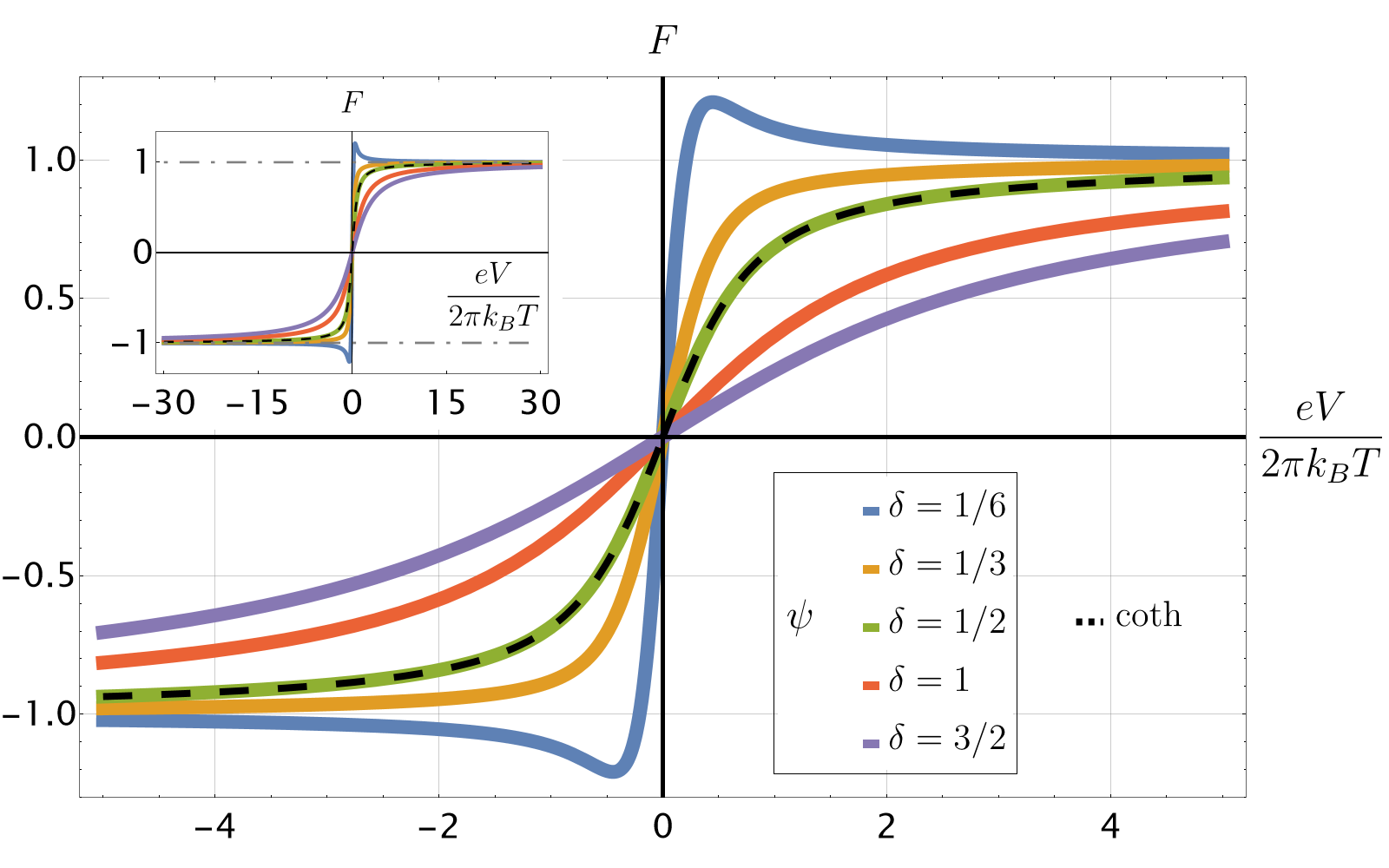
The Fano factor in the regime of weak quasiparticle tunnelling turns out to be an ideal candidate for performing such a check. One can write the universal answer for any model within the CLL framework [2, 44, 45]:
| (1) |
where denotes the imaginary part, and is the digamma function. Equation (1) recreates the asymptotic shot noise limit, for . Yet, when and are comparable, the formula enables extracting the scaling dimension alongside the quasiparticle charge . There exist non-idealities that lead to a renormalization of the scaling dimension (such as the ones mentioned above) — yet they do not change Eq. (1) unless they break the CLL. Further, Eq. (1) is not sensitive to the tunnelling amplitude at the QPC, which may exhibit non-universal dependence on the system parameters (such as or ).
The most important feature of Eq. (1) for the present work is the scaling behaviour: The Fano factor depends only on the ratio , and not on or separately. Therefore, the Fano factor data measured at different temperatures should collapse on top of each other when plotted as a function of this dimensionless ratio. In fact, this prediction can be expected even without reference to the CLL: as long as and are the only relevant energy scales, the dimensionless Fano factor can only depend on their dimensionless ratio.
Conversely, the collapse may not be observed in the presence of other energy scales. The bulk gap is one such energy scale, yet other scales may exist.
In this work, we perform experiments at . We measure the noise and the differential conductance in the QPC tunnelling processes at several temperatures, and then analyze the data using Eq. (1). We first verify the scaling behaviour of the Fano factor. We find a partial data collapse, hinting at the violation of CLL behaviour. The region where the scaling behaviour does hold, corresponds to . The data in this region only enable extracting a combination of and , and not each of them separately. Assuming the value of , as known from experiments of other types [40, 41, 42, 43], we extract the value of . This value is drastically different from the naïve CLL prediction of for .
Our results suggest the existence of physical effects leading to scaling dimension renormalization, and to generation of additional energy scales which lead to the CLL violation significantly below the bulk gap. We identify electrostatic interactions at the QPC as a likely culprit.
Most importantly, the present firm observation of the breakdown of the CLL and of the scaling dimension renormalization in the CLL-compatible regime opens a way to reconcile various experimental results on QPC tunnelling with the CLL theory of fractional quantum Hall edges in a systematic manner. Ad-hoc modifications to the theory can now be replaced with separating CLL-compatible and CLL-incompatible regions of data. Furthermore, our method opens a new window into the mesoscopic world physics by allowing quantitative studies of scaling dimension renormalization.
II Results
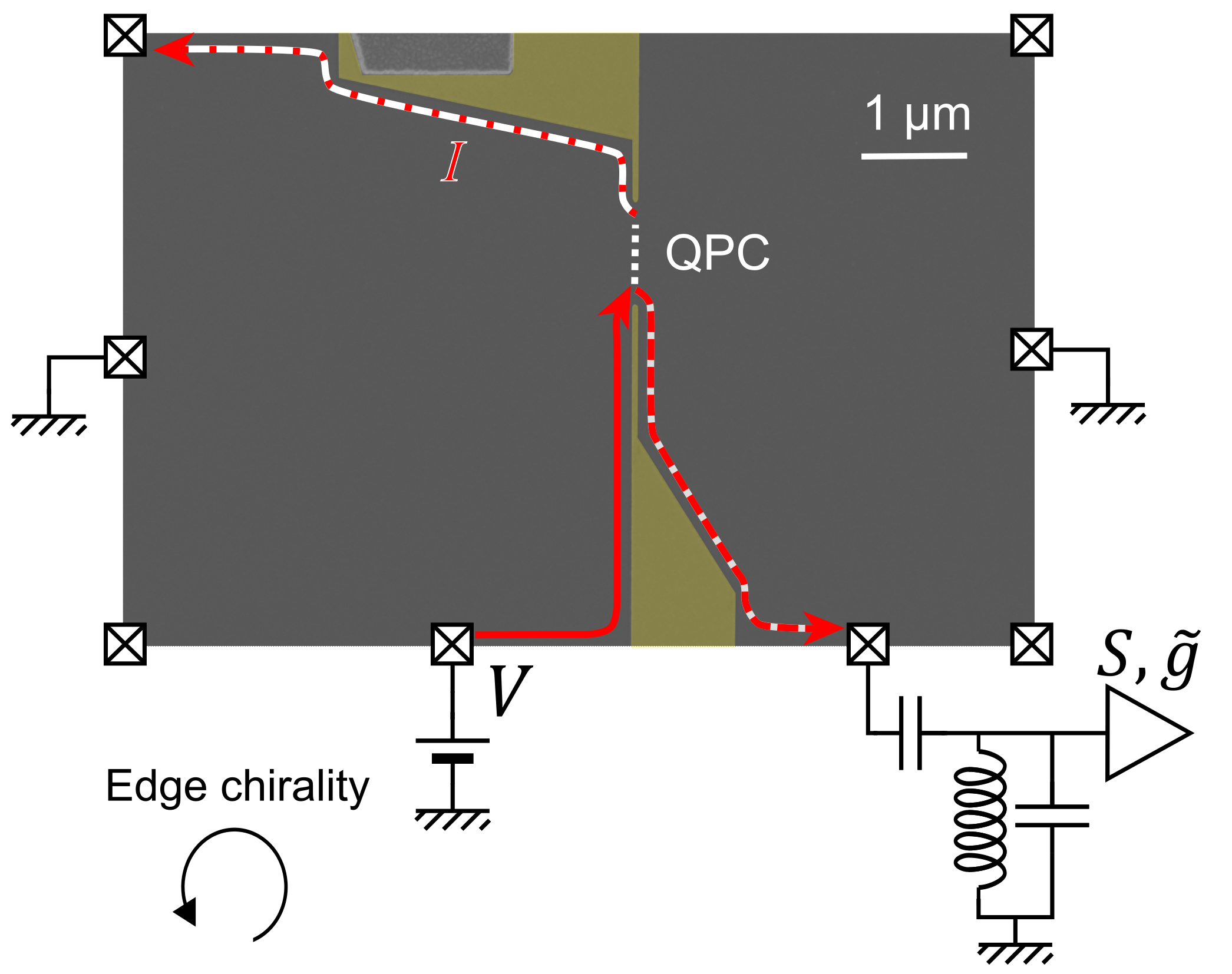
We perform standard measurements of the tunnelling current and noise generated due to quasiparticle tunnelling at , as shown in Fig. 1. The source contact is placed at bias voltage , emitting a chirally propagating current, shown as a red line. This current arrives at a QPC, where it is partitioned. An amplifier is connected to the Ohmic contact downstream from the QPC, enabling the measurement of the excess222“Excess” means the noise with the Johnson-Nyquist noise (the noise measured at ) subtracted. auto-correlation noise and the differential conductance , where is the tunnelling current leaking from the edge via the QPC and is the differential tunnelling conductance. The Fano factor, , is calculated based on these data. All the measurements have been performed on a 2D electron gas embedded in a GaAs/AlGaAs heterostructure, with an areal density of and mobility at 4 K temperature, on which the QPC was fabricated. Additional data on the sample, fabrication and measurement is given in the Methods section.
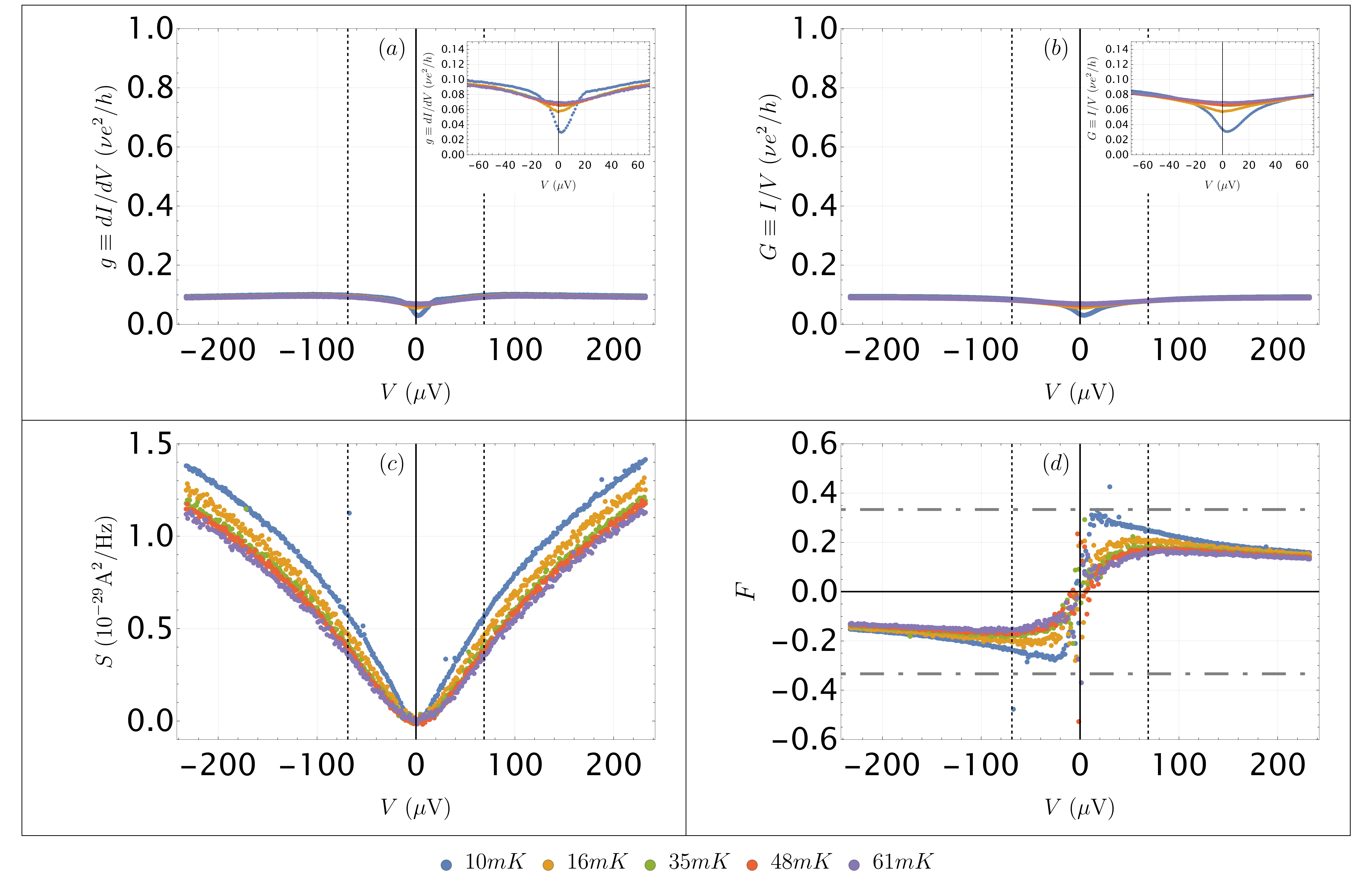
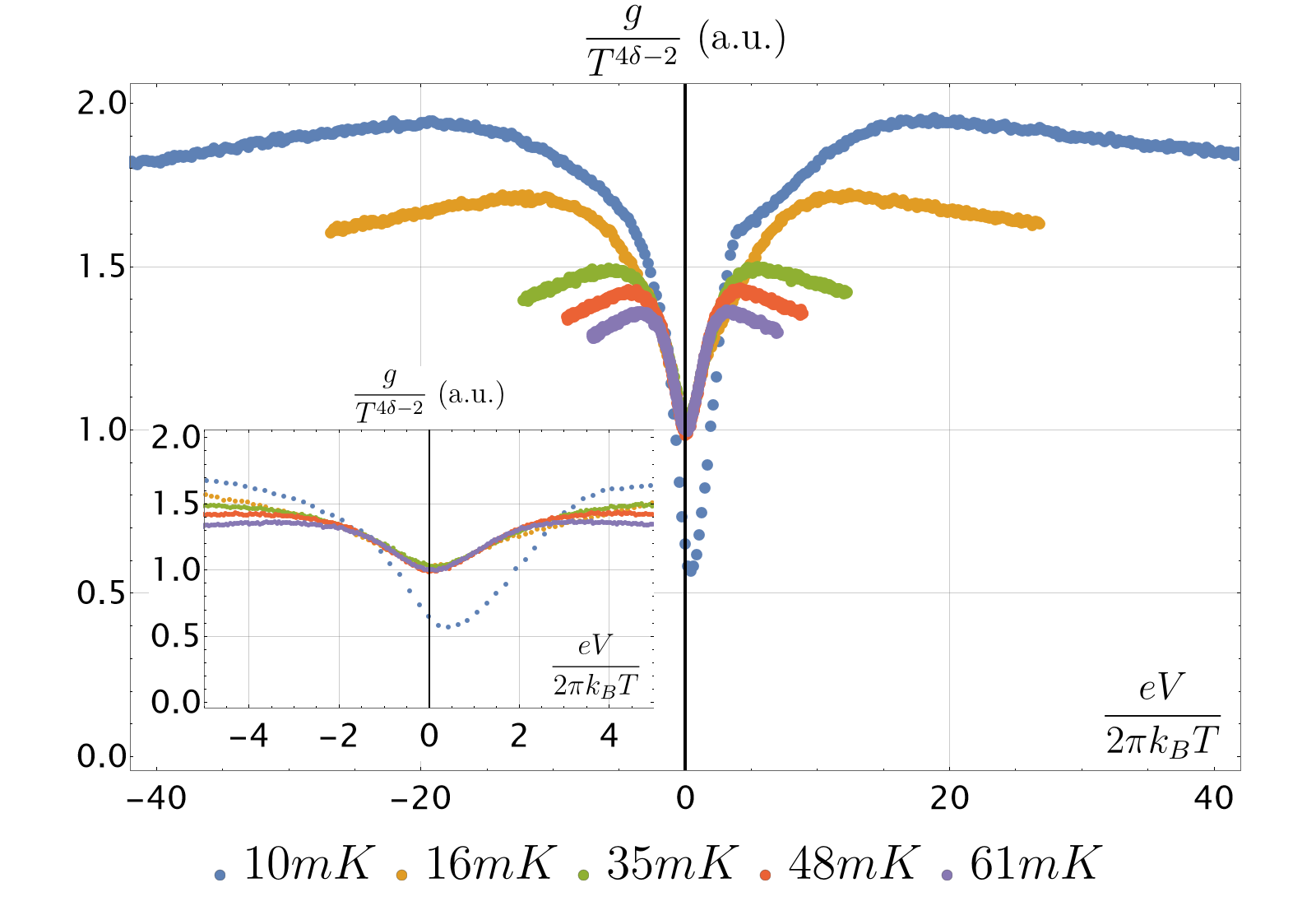
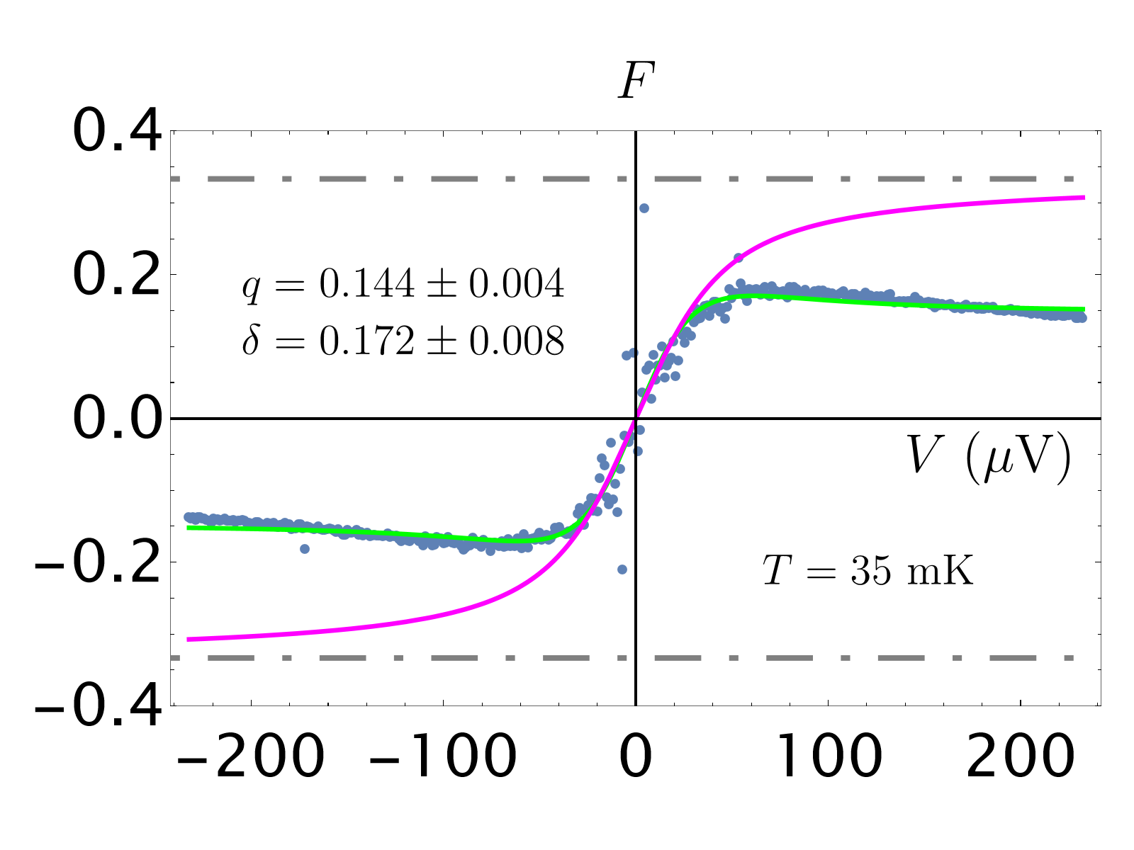
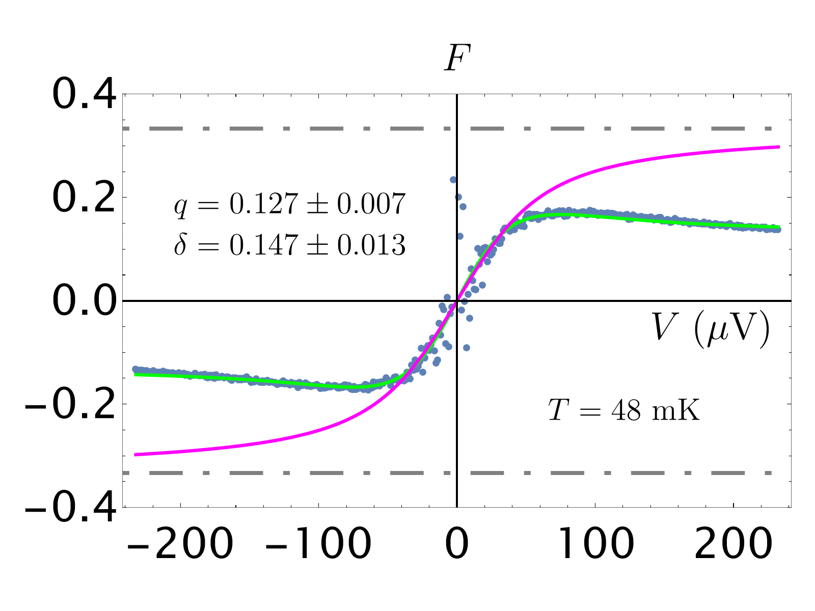
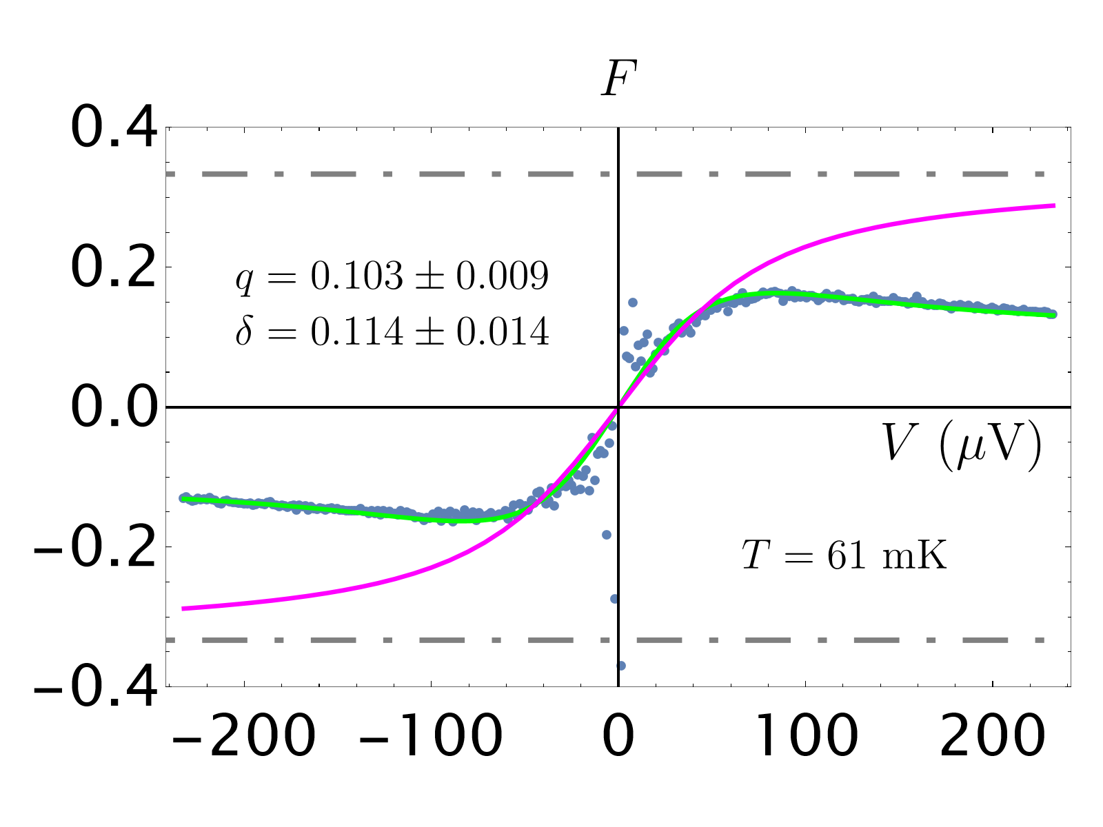
The measurements are performed at five different temperatures of the sample. The electron temperature has been inferred from the Johnson-Nyquist noise measurement (i.e., at vanishing bias voltage, ). The raw data for the differential conductance and the excess noise are presented in Fig. 2(a,c). Note that for all data points , indicating a regime of weak quasiparticle tunnelling, in which Eq. (1) is expected to be valid. Based on the raw data, the integral conductance and the Fano factor are calculated, see Fig. 2(b,d).
Note that the theoretical prediction for the Fano factor in the regime of large , , is in stark contrast with the experimental observations. This discrepancy was observed even in the earliest Fano-factor-based measurements of the fractional charge, cf. [Figs. 3, 4 in 7] and [Figs. 2, 3 in 8]. We will come back to this issue in the Discussion section. For the moment, we only remark that the raw experimental data do not contain a regime of the Fano factor leveling off at for an extended range of voltages, in contradiction with the conventional expectation by theorists.
As stated in the introduction, the primary model-independent test for CLL behaviour is the scaling property of the Fano factor. The scaled data for the Fano factor are presented in Fig. 3. We observe the data collapse for , whereas beyond that region the scaling fails. The three higher-temperature curves seem to collapse well up to a higher cutoff of , yet also part from each other outside that region. These deviations from the expected scaling behaviour hint at a violation of CLL behaviour at an energy scale of the order . Here is the breakdown point of the scaling; the K estimate is produced using and mK; the K estimate follows from taking and mK. Note that even K is significantly below the bulk gap scale K (the estimate is taken as the smallest gap for measured in Refs. [46, 47]). One is forced to conclude that an important additional energy scale (perhaps, several) is present below the bulk gap.
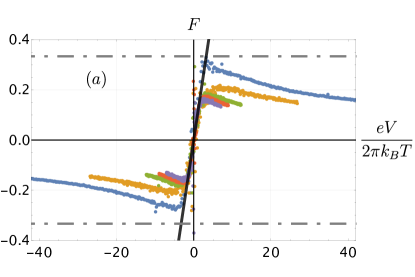

Henceforth, we focus on the region of sufficiently small , where scaling behaviour is observed and which can thus be compatible with the CLL. The collapsed data are linear in , which corresponds to the regime of in Eq. (1), where it can be approximated as
| (2) |
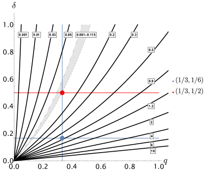
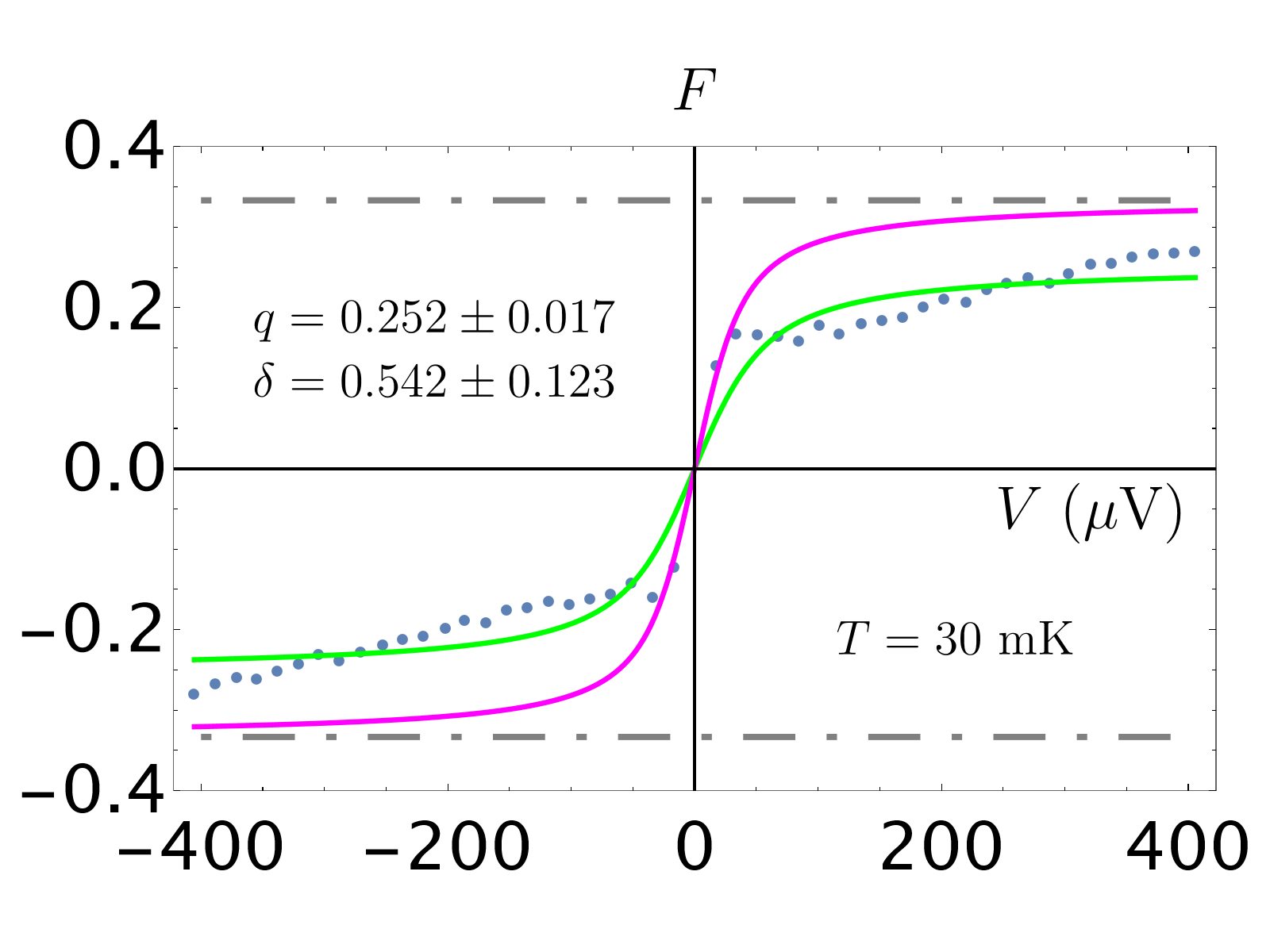
This implies that the data in this regime do not allow for extracting the quasiparticle charge and scaling dimension individually, only their combination. We fit the data and extract the slope (95% confidence). Figure 4 displays contours for different values of in the plane; the region compatible with the extracted slope is highlighed in grey. Notably, the pristine theoretical prediction for the Laughlin edge, , is incompatible with this curve. Assuming that the quasiparticle charge is (as evidenced by multiple experiments [40, 41, 42, 43]), one extracts .
It is worth elaborating further on the particular value of extracted above. The CLL predicts the tunnelling current to behave as
| (3) |
where is the Euler’s gamma function and encodes the bare tunnelling amplitude for quasiparticles at the QPC (see Refs. [15, 16, 17, 18, 19] for the original derivation and Refs. [48, 29, 44] for the expression in the notation close to the present one). In the regime , this reduces to
| (4) |
The differential conductance is predicted to exhibit a zero-bias peak for and a zero-bias dip for . The value of is associated with . This is compatible with the behaviour seen in Fig. 2(a) (in fact, the zero bias dip at small voltage is compatible with the value slightly above 1/2, which we have extracted).
This correspondence between the scaling dimension and the differential conductance could, in principle, be spoiled. The tunnelling amplitude could have a dependence of the bias voltage , due to electrostatic interactions in the sample forcing the QPC edges to change their location depending on the bias voltage. This would transform Eq. (4) to be , and the differential conductance would acquire an additional non-universal contribution , disallowing one to make conclusions about the scaling dimension from the tunnelling conductance alone. The fact that the scaling dimension extracted from the Fano factor also enables explaining the behaviour of is thus an evidence that dependence can be neglected. If one assumes that such a statement has general applicability, one obtains additional means of verifying the value of independently.
III Discussion
The above results provide clear evidence for heavy renormalization of the scaling dimension and provide an experimental method for its quantitative investigation. However, the implication of these results is much more significant, as it enables reconciliation of multiple experimental results and theoretical efforts of the last 25+ years. Below, we discuss various aspects of those links and interconnections.
III.1 Relation to other tunnelling current experiments
The obtained value of may seem quite arbitrary. However, the appearance of this specific value has deep ties to how Fano factor experiments have been performed. In a typical experimental sample, the observed dependences of the differential conductance on the bias voltage change from zero-bias peaks to zero-bias dips as a function of the voltage of the gates that confine the QPC, see, e.g., [Figs. 3, 5 in 22] or [Fig. S3c in the SM of 11]. With the few exceptions we will discuss below, past experiments have focused on the regime of as flat as possible. This practical choice has two reasons. First, the CLL predictions are well controlled in the regime when the tunnelling conductance is small (); satisfying this requirement for the whole range of is easiest when the dependence is flat. Second, this choice is influenced by the intuition coming from dealing with the Fermi liquid; non-interacting free fermions can be described with CLL using , again predicting flat ; with such intuition, deviation from this behaviour may raise suspicions of non-universal behaviour of the tunnelling amplitude at the QPC — a good thing to avoid, when trying to verify universal predictions.
Therefore, obtaining appears to be a consequence of deliberate preference for using the data with flat . One implication of the above is that the data with non-flat transmission, which are typically ignored, can be analyzed with the help of our method. This analysis would allow for a systematic study of the scaling dimension renormalization in the QPCs.
While experiments aiming at extracting the Fano factor have historically focused on flat , there have been a number of experiments aiming to measure the CLL-predicted zero-bias peak, [Fig. 3c in 22] and [29, 30, 31, 32, 33]. These experiments used the data in the regime where exhibits a zero-bias peak. They found good agreement between the theory prediction (3) and the experimental data at sufficiently small bias voltages , yet deviations from the predicted behaviour at larger . The results of our analysis suggest that these deviations are due to the violation of CLL behaviour we find at sufficiently large energies.
Further, some experiments hunting for the zero-bias peak [31, 32, 33] have made ad-hoc adjustments to the theory by adding an extra constant to , in order to account for flat transmission at high . This enabled extracting the values of and by fitting the experimental data with modified formulas. However, the extracted values never fully coincide with the theory predictions for . Our results suggest a better way to analyse the data: cut out the region of where CLL is no longer valid (where scaling of the Fano factor fails) and analyze the data without making ad-hoc adjustments. Indeed, we show in the Supplemental Material [49] that ignoring the CLL breakdown can lead to data fits of excellent quality, yet with wrong and even temperature-dependent values of .
Finding the appropriate region of to analyze constitutes a challenge when data only at one temperature are available. Having the data at several temperatures, however, makes this possible.
A recent work [34] has pointed out that CLL predicts scaling behaviour for and verified this behaviour in a FQH QPC in graphene.333Admittedly, such behaviour was demonstrated in a rather exotic situation: electron tunnelling between the edges of different filling factors. Note, however, that such results have not been demonstrated so far for quasiparticle or electron tunnelling between the edges of the same filling factor. This method assumes that the tunnelling amplitude does not exhibit non-universal dependence . Under this assumption, this method enables determining the energy scale of CLL violation similarly to ours. Combining the two methods, would allow a powerful experimental methodology with internal cross-checks. In the Supplementary material [49], we demonstrate that this method works with our data for all temperatures except the lowest one. This may indicate the importance of excluding the influence of via our Fano factor scaling technique.
III.2 Scaling dimension renormalization
The scaling dimension we find, , is clearly distinct from the naïve CLL prediction of for the Laughlin edge at . This on its own, however, does not invalidate the CLL framework for describing quantum Hall edges. Over the years, theorists proposed a number of effects that can lead to scaling dimension renormalization. First and foremost, the same filling factor admits multiple edge models [1] that can have a different number of edge modes, different spectrum of quasiparticles, and the elementary quasiparticle in those models can differ in charge, statistics, and scaling dimension. Further, in the presence of counterpropagating edge modes, the scaling dimension of a quasiparticle can change due to electrostatic interactions between those edge modes [50, 51, 52]. Finally, even the simplest edges allow for scaling dimension renormalization locally, in the vicinity of a QPC due to interactions across the elements of the QPC [23, 24, 25].
The continuous change of shape of the differential conductance curves as a function of the QPC confining voltage, see [Figs. 3, 5 in 22] and [Fig. S3c in the SM of 11], suggests that the latter mechanism plays the dominant role in QPC experiments. The method proposed above enables quantitative experimental studies of scaling dimension renormalization.
Back-of-the envelope estimates for CLL breakdown scale also speak in favour of this mechanism. In our sample, the distance along which the incoming and outgoing parts of the edge at the QPC are close to each other is on the order of , cf. Fig. 1. This is the region where one can expect the Coulomb interaction between the edges to be strong, which renormalizes the scaling dimension. The pattern of renormalization should, however, depend on the energies concerned [25, 53]: for energies up to , the wavelength of incoming quasiparticles is larger than , while for , the wavelength fits completely within the region of strong Coulomb interactions. One, therefore, expects a change of renormalization pattern and thus CLL breaking around . Taking [54] and , one estimates . This order-of-magnitude estimate agrees surprisingly well with the CLL breakdown scale () extracted from the experimental data.
As for detailed theory predictions of the renormalization, it is possible to predict the scaling dimension using CLL if one knows the strength of electrostatic interactions across the QPC [23, 24, 25]. Coincidentally, numerical methods developed recently allow for quantitatively accurate predictions of the electrostatic behaviour of mesoscopic devices [55, 56]. Combining these analytical and numerical methods together, it should be possible to derive predictions for the QPC behaviour based solely on the knowledge of the material properties and device geometry.
III.3 Interpreting the quasiparticle charges reported previously based on the Fano factor
As stated above, the theoretical expectation that the Fano factor at sufficiently large bias voltage becomes the quasiparticle charge, , does not hold in actual experiment. This raises the question: what should one think of the previously reported fractional charges extracted from the Fano factor experiments at various filling factors?
Providing an answer to the question requires a close look at the methodology that was used to extract those values of . The conventional methodology is as follows [e.g., 57, 39]: tune the QPC to the regime of flattest possible differential conductance dependence and analyze the experimental data using a phenomenological Fermi-liquid-inspired formula,
| (5) |
This formula has the expected behaviour of when and . The formula does not have any dependence on the scaling dimension , making it less general than Eq. (1), cf. Fig. 5. However, for Eq. (1) reduces to Eq. (5) taken in the limit . Note that corresponds to free non-interacting fermions, but it also describes fractional quasiparticles whose scaling dimension was renormalised to the value of . Given the results of our analysis above, it stands to reason that tuning to be flat corresponds to tuning to be . Therefore, by serendipity, the use of Eq. (5) in this context is justified and expected to return the correct value of .
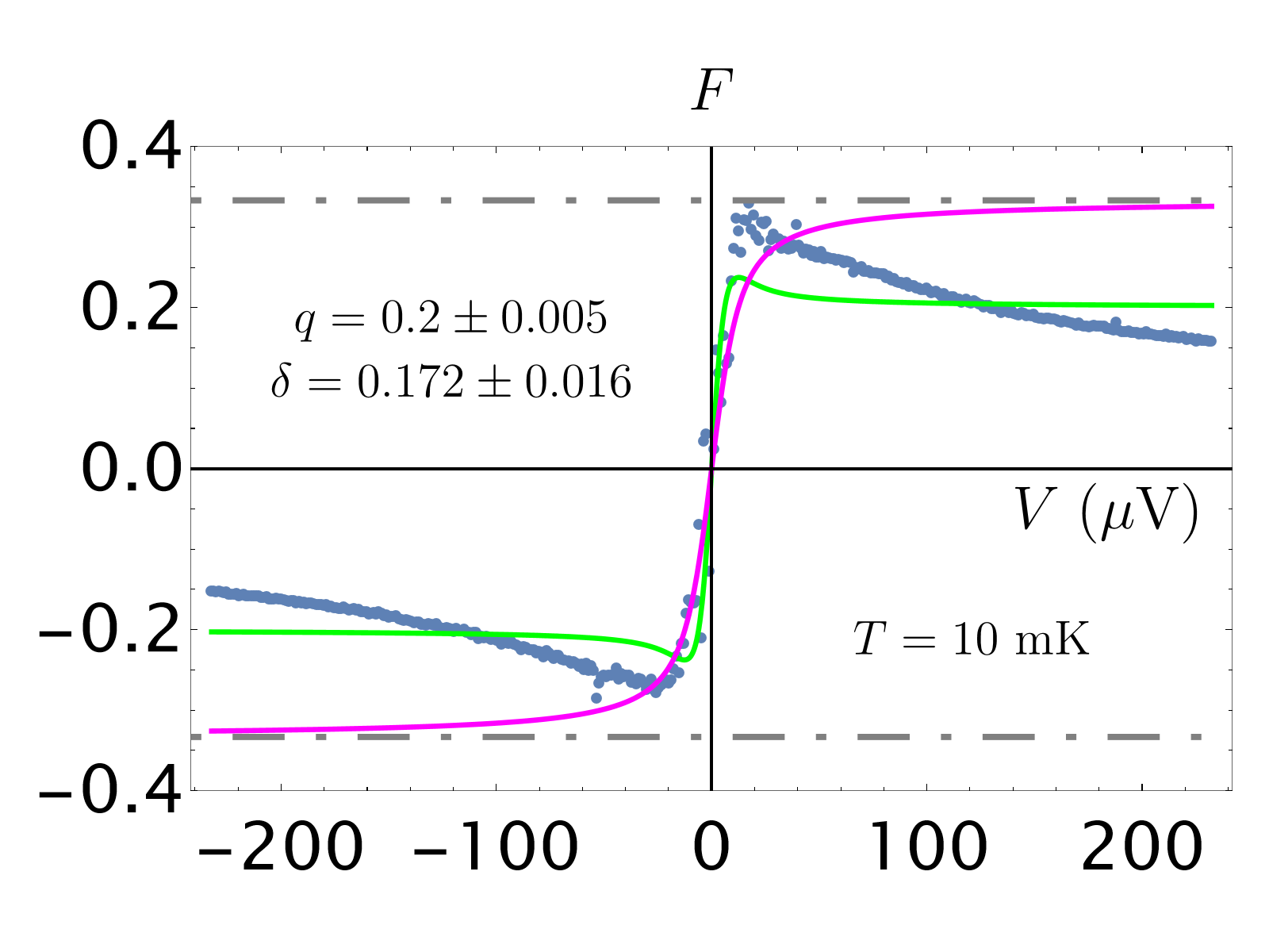
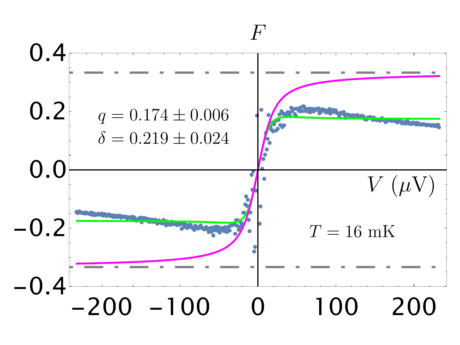
Concerning the unexpected large- behaviour of the Fano factor, such behaviour has also been observed in the past. See, e.g., Refs. [Figs. 3, 4 in 7] and [Figs. 2, 3 in 8] — it is widespread, and not specific to the present experiment. The only behaviour of the Fano factor allowed by Eq. (5) is for the Fano factor to level off after the initial period of growth, cf. Fig. 5. Therefore, the Fano factor bending down as in Fig. 2(c) was a reason to believe that the theory has stopped working at this energy scale and the data for a limited range of should be analysed. Coincidentally, this happens around the same place where the scaling behaviour breaks down. Given the tuning to discussed above, this analysis of the truncated data — using Eq. (5) — leads to the same results as in our more general methodology. At the same time, we stress that for this intuition would be misleading and could lead to discarding valid data in the CLL regime, cf. Fig. 5.
Interestingly, there have been theoretical attempts to justify the use of Eq. (5) or similar coth-based formulas for noise analysis [58, 59]. We believe that these theory arguments are correct, but require careful interpretation. First, we note that the predictions of Eq. (5) are clearly distinguishable from those of Eq. (1) in principle (as evidenced by Fig. 5) and in practice. Indeed, Fig. 4 shows that the naive CLL prediction of is clearly excluded by the experimental data, while is not.
Second, the two references [58, 59] explicitly have in their coth-based formulas444For example, through using Eq. (1) outside the regime — but also in other ways within regime. and assume no voltage dependence of the tunnelling amplitude . The use of experimentally measured is then implied. This calls for an explanation: how is it possible that the noise predictions of the theory agree well with the coth-based formula, which in turn agrees well with the experimental data — yet the experimental does not coincide with the theoretical ? What is the mechanism for agreement of a data set “noise + tunnelling current” with the theory, whereas the subset “tunnelling current” does not agree with the underlying theory? This question is fully applicable to Ref. [58]. Reference [59] avoids this criticism by deriving its theory from statistical mechanics — thus making no reference to the CLL and not making any prediction for . Our analysis shows that this question is resolved within the CLL framework by scaling dimension renormalization. The renormalization provides a natural explanation for the success of Eq. (5) — given the experimental tuning of to flattness.
Further, the scaling dimension renormalization provides an explanation for why it is possible to find flat systematically, when tuning the QPC transparency. As discussed in Sec. III.2, interaction of the edges in the vicinity of the QPC are likely to be the mechanism for the renormalization. Adjusting the voltage of the gates controlling the QPC changes the positions of the edges, changing the interaction strength, thence the scaling dimension. Note, that other non-universalities (such as dependence) are unlikely to produce flat .
We stress that our method proposed in this work enables the analysis of the data at non-flat , significantly extending the pool of interpretable experimental data. One can now systematically analyze within the CLL framework the data that have typically been unexplained and discarded.
The above discussion shows that the previously reported values of fractional charges obtained in Fano factor experiments may often be trustworthy. However, since the data analysis methodology may differ from work to work, one should look into the analysis details in order to confirm this. In the Supplemental Material [49], we provide an example of non-trustworthy charge extraction: we perform a naive analysis of our above experimental data using Eq. (1) in the full voltage range, ignoring the CLL breakdown — this leads to data fits of excellent quality with wrong and temperature-dependent values of . Therefore, being pedantic about the data analysis methodology is crucial for understanding FQH QPC tunnelling experiments.
III.4 Violation of CLL scaling behaviour: ubiquity and possible mechanisms
It is reasonable to ask whether the CLL breakdown observed in our QPC is unique to the specific sample or to the filling factor of , or occurs ubiquitously. The data peresent in the literature do not allow one to fully answer this question due to the lack of data for the Fano factor at multiple temperatures in the same sample. However, we have performed the analysis of the single-temperature data available from recent Refs. [42, 11] and we find signatures similar to the ones observed in our data, suggesting that the CLL breakdown is a ubiquitous phenomenon. We present details of this analysis in the Supplemental Material [49].
In fact, expecting the CLL picture to break down is only natural from the theory point of view. As stated in the introduction, it only takes an additional energy scale to destroy the CLL-predicted scaling property. One such energy scale is the bulk gap of the FQH sample — as soon as one has access to such energies, one cannot focus on the edge and should include bulk dynamics into consideration. However, we observe the breakdown at an energy scale about 4–40 times smaller than the bulk gap.
One can imagine a number of possible mechanisms that could lead to the breakdown of CLL predictions with edge physics only. To mention but a few: (i) non-linear dispersion of edge modes [60], (ii) energy dependence of the bare tunnelling amplitude, (iii) energy-dependent renormalization of the scaling dimension. A systematic investigation of these mechanisms goes way beyond the scope of the present work. In Sec. III.2 above, we showed that mechanism (iii) predicts the correct CLL breakdown scale — yet we did not analyze the Fano factor beyond the breakdown scale. In the Supplemental Material [49], we provide a toy model mimicking mechanism (iii) and show that it can lead to the qualitative behaviour observed: the Fano factor value at large being significantly smaller than the quasiparticle charge .
IV Conclusions
In this paper, we have introduced a new framework to analyze decades-old experiments concerning quasiparticle tunnelling in the FQH effect. Despite apparent success in determining the fractional quasiparticle charge, the correspondence between theory and experiments across the whole set of FQH investigations performed was unsatisfactory. Our new methodology bridges this gap and opens the way to reconciliating multiple quasiparticle tunnelling experiments systematically.
Our methodology is based on investigating the scaling behaviour of the Fano factor as a function of bias voltage and system temperature. This enables us to obtain clear signatures of CLL breakdown is some experimental regimes and extract the quasiparticle scaling dimension in others.
In the outlook, our methodology opens two new directions: One can perform quantitative studies of scaling dimension renormalization and thus get insight into the physics of mesoscopic devices. Simultaneously, one can investigate the breakdown of CLL at quantum Hall edges in order to get further insights into real-world, non-idealized physics of topological matter.
Acknowledgements
KS acknowledges illuminating discussions with Gwendal Fève, Christophe Mora, Christian Glattli, Inès Safi, Frédéric Pierre, and Bernd Rosenow, and thanks numerous other people working in the field for small and big discussions over the last 15 years. K.S. acknowledges funding by the Deutsche Forschungsgemeinschaft (DFG, German Research Foundation): Projektnummer 277101999, TRR 183 (Project No. C01), Projektnummer GO 1405/6-1, Projektnummer MI 658/10-2, by the German-Israeli Foundation Grant No. I-1505-303.10/2019, as well as funding from the European Union’s Horizon 2020 research and innovation programme under grant agreement No. 862683 (UltraFastNano). M.H. acknowledges the support of the European Research Council under the European Union’s Horizon 2020 research and innovation programme (grant agreement number 833078). This paper was prepared with the help of LyX editor.
Note added.
We have become aware of two experimental works addressing the question of scaling dimension of quasiparticle in FQH effect. The one performed in the group of F. Pierre (A. Veillon et al., [61]) analyses data for the Fano factor with the CLL theoretical prediction of Eq. (1), yet without scaling analysis; it finds in multiple independent QPCs and at multiple temperatures. Another is performed in the group of G. Fève (M. Ruelle et al., submitted to a journal); this work uses a different method (proposed in Ref. [62]) and finds . The differences between we find and the scaling dimensions found in these works provide further evidence to the non-universal effects of scaling dimension renormalization discussed above. In light of the findings detailed in our present work, performing a scaling analysis, in particular, examining whether the data exhibit a similar CLL breakdown, would be important to confirm the relevance of our findings to these works.
Methods
Sample and device fabrication. The sample was fabricated on a uniform doping GaAs/AlGaAs heterostructure with a 2-dimensional electron gas formed 118 nm underneath the surface. The transport properties of the 2DEG showed the density with mobility at temperature . The wet etching technique defined electronic mesa around the QPC site, and e-gun evaporation of a metallic stack of Ge/Ni/Au was used to form the Ohmic contacts. The metallic gates that define the QPC were deposited on the layer using e-beam lithography (JEOL, JBX-9300FS) and metal evaporation of Ti/Au. The Hafnia layer was etched using /Ar gas, and Ti/Au contact lead was deposited. All the processes except QPC patterning used the optical lithography methods using laser writer (Heidelberg Instruements, DWL 66+).
Measurement. The device was placed on a mixing chamber plate cold-finger part in a commercial wet dilution refrigerator (Leiden Cryogenics, Minikelvin 126-TOF). Differential conductance measurements were done via lock-in technique using a lock-in amplifier (NF corporation, LI5655). The shot noise was amplified by ATF-34143 HEMT-based homemade low-temperature voltage amplifier with battery-powered DC source (Standard Research Systems, SIM928) and NF corporation SA-220F5 room temperature voltage amplifier (second amplifying). The noise was then demodulated by the lock-in amplifier bandwidth open method (Zurich instruments, MFLI).
Author contributions
N.S., Y.O., and K.S. conceived the experiment. N.S. and K.S. performed the data analysis. T.A. and C.H. contributed to the device design, fabrication, and measurements. V.U. has grown the sample with molecular-beam epitaxy. N.S., T.A., C.H., M.H., Y.O., and K.S. participated in discussions of the results and their interpretation.
Data availability
The raw experimental data used in this work and the Mathematica code that performs the analysis and produces the figures are available at https://doi.org/10.5281/zenodo.10840561.
References
- Wen [2007] X.-G. Wen, Quantum Field Theory of Many-Body Systems: From the Origin of Sound to an Origin of Light and Electrons (Oxford University Press, 2007).
- Schiller et al. [2022] N. Schiller, Y. Oreg, and K. Snizhko, Extracting the scaling dimension of quantum Hall quasiparticles from current correlations, Physical Review B 105, 165150 (2022).
- Stern [2008] A. Stern, Anyons and the quantum Hall effect - a pedagogical review, Annals of Physics 323, 204 (2008), arXiv:0711.4697 .
- Laughlin [1983] R. B. Laughlin, Anomalous Quantum Hall Effect: An Incompressible Quantum Fluid with Fractionally Charged Excitations, Physical Review Letters 50, 1395 (1983).
- Arovas et al. [1984] D. Arovas, J. R. Schrieffer, and F. Wilczek, Fractional Statistics and the Quantum Hall Effect, Physical Review Letters 53, 722 (1984).
- Moore and Read [1991] G. Moore and N. Read, Nonabelions in the fractional quantum hall effect, Nuclear Physics B 360, 362 (1991).
- de-Picciotto et al. [1997] R. de-Picciotto, M. Reznikov, M. Heiblum, V. Umansky, G. Bunin, and D. Mahalu, Direct observation of a fractional charge, Nature 389, 162 (1997).
- Saminadayar et al. [1997] L. Saminadayar, D. C. Glattli, Y. Jin, and B. Etienne, Observation of the e / 3 Fractionally Charged Laughlin Quasiparticle, Physical Review Letters 79, 2526 (1997).
- Dolev et al. [2008] M. Dolev, M. Heiblum, V. Umansky, A. Stern, and D. Mahalu, Observation of a quarter of an electron charge at the = 5/2 quantum Hall state, Nature 452, 829 (2008).
- Nakamura et al. [2020] J. Nakamura, S. Liang, G. C. Gardner, and M. J. Manfra, Direct observation of anyonic braiding statistics, Nature Physics 16, 931 (2020).
- Bartolomei et al. [2020] H. Bartolomei, M. Kumar, R. Bisognin, A. Marguerite, J.-M. Berroir, E. Bocquillon, B. Plaçais, A. Cavanna, Q. Dong, U. Gennser, Y. Jin, and G. Fève, Fractional statistics in anyon collisions, Science 368, 173 (2020).
- Lee et al. [2023] J.-Y. M. Lee, C. Hong, T. Alkalay, N. Schiller, V. Umansky, M. Heiblum, Y. Oreg, and H.-S. Sim, Partitioning of diluted anyons reveals their braiding statistics, Nature 617, 277 (2023).
- Ruelle et al. [2023] M. Ruelle, E. Frigerio, J.-M. Berroir, B. Plaçais, J. Rech, A. Cavanna, U. Gennser, Y. Jin, and G. Fève, Comparing Fractional Quantum Hall Laughlin and Jain Topological Orders with the Anyon Collider, Phys. Rev. X 13, 011031 (2023), arXiv:2210.01066 .
- Glidic et al. [2023] P. Glidic, O. Maillet, A. Aassime, C. Piquard, A. Cavanna, U. Gennser, Y. Jin, A. Anthore, and F. Pierre, Cross-Correlation Investigation of Anyon Statistics in the and Fractional Quantum Hall States, Phys. Rev. X 13, 011030 (2023), arXiv:2210.01054 .
- Wen [1991] X.-G. Wen, Edge transport properties of the fractional quantum Hall states and weak-impurity scattering of a one-dimensional charge-density wave, Physical Review B 44, 5708 (1991).
- Kane and Fisher [1992a] C. L. Kane and M. P. A. Fisher, Transport in a one-channel Luttinger liquid, Physical Review Letters 68, 1220 (1992a).
- Kane and Fisher [1992b] C. L. Kane and M. P. A. Fisher, Transmission through barriers and resonant tunneling in an interacting one-dimensional electron gas, Physical Review B 46, 15233 (1992b).
- de C. Chamon and Wen [1993] C. de C. Chamon and X. G. Wen, Resonant tunneling in the fractional quantum Hall regime, Physical Review Letters 70, 2605 (1993).
- Kane and Fisher [1994] C. L. Kane and M. P. A. Fisher, Nonequilibrium noise and fractional charge in the quantum Hall effect, Physical Review Letters 72, 724 (1994).
- Fendley et al. [1994] P. Fendley, H. Saleur, and N. P. Warner, Exact solution of a massless scalar field with a relevant boundary interaction, Nuclear Physics B 430, 577 (1994), arXiv:hep-th/9406125 .
- Fendley et al. [1995] P. Fendley, A. W. W. Ludwig, and H. Saleur, Exact nonequilibrium transport through point contacts in quantum wires and fractional quantum Hall devices, Physical Review B 52, 8934 (1995).
- Heiblum [2006] M. Heiblum, Quantum shot noise in edge channels, physica status solidi (b) 243, 3604 (2006).
- Pryadko et al. [2000] L. P. Pryadko, E. Shimshoni, and A. Auerbach, Coulomb interactions and delocalization in quantum Hall constrictions, Physical Review B 61, 10929 (2000).
- Papa and MacDonald [2004] E. Papa and A. H. MacDonald, Interactions Suppress Quasiparticle Tunneling at Hall Bar Constrictions, Physical Review Letters 93, 126801 (2004).
- Yang and Feldman [2013] G. Yang and D. E. Feldman, Influence of device geometry on tunneling in the quantum Hall liquid, Physical Review B 88, 085317 (2013).
- Braggio et al. [2012] A. Braggio, D. Ferraro, M. Carrega, N. Magnoli, and M. Sassetti, Environmental induced renormalization effects in quantum Hall edge states due to 1/ f noise and dissipation, New Journal of Physics 14, 093032 (2012).
- Rosenow and Halperin [2002a] B. Rosenow and B. I. Halperin, Nonuniversal Behavior of Scattering between Fractional Quantum Hall Edges, Physical Review Letters 88, 096404 (2002a).
- Ferraro et al. [2008] D. Ferraro, A. Braggio, M. Merlo, N. Magnoli, and M. Sassetti, Relevance of Multiple Quasiparticle Tunneling between Edge States at = p / ( 2 n p + 1 ), Physical Review Letters 101, 166805 (2008).
- Roddaro et al. [2003] S. Roddaro, V. Pellegrini, F. Beltram, G. Biasiol, L. Sorba, R. Raimondi, and G. Vignale, Nonlinear Quasiparticle Tunneling between Fractional Quantum Hall Edges, Physical Review Letters 90, 046805 (2003).
- Roddaro et al. [2004] S. Roddaro, V. Pellegrini, F. Beltram, G. Biasiol, and L. Sorba, Interedge Strong-to-Weak Scattering Evolution at a Constriction in the Fractional Quantum Hall Regime, Physical Review Letters 93, 046801 (2004).
- Radu et al. [2008] I. P. Radu, J. B. Miller, C. M. Marcus, M. A. Kastner, L. N. Pfeiffer, and K. W. West, Quasi-Particle Properties from Tunneling in the = 5/2 Fractional Quantum Hall State, Science 320, 899 (2008).
- Lin et al. [2012] X. Lin, C. Dillard, M. A. Kastner, L. N. Pfeiffer, and K. W. West, Measurements of quasiparticle tunneling in the fractional quantum Hall state, Physical Review B 85, 165321 (2012).
- Rössler et al. [2014] C. Rössler, T. Ihn, K. Ensslin, C. Reichl, W. Wegscheider, and S. Baer, Experimental probe of topological orders and edge excitations in the second Landau level, Physical Review B 90, 075403 (2014).
- Cohen et al. [2023] L. A. Cohen, N. L. Samuelson, T. Wang, T. Taniguchi, K. Watanabe, M. P. Zaletel, and A. F. Young, Universal chiral Luttinger liquid behavior in a graphene fractional quantum Hall point contact, Science 382, 542 (2023), arXiv:2212.01374 .
- Griffiths et al. [2000] T. G. Griffiths, E. Comforti, M. Heiblum, A. Stern, and V. Umansky, Evolution of Quasiparticle Charge in the Fractional Quantum Hall Regime, Physical Review Letters 85, 3918 (2000).
- Chung et al. [2003] Y. C. Chung, M. Heiblum, and V. Umansky, Scattering of Bunched Fractionally Charged Quasiparticles, Physical Review Letters 91, 216804 (2003).
- Bid et al. [2010] A. Bid, N. Ofek, H. Inoue, M. Heiblum, C. L. Kane, V. Umansky, and D. Mahalu, Observation of neutral modes in the fractional quantum Hall regime, Nature 466, 585 (2010).
- Snizhko [2016] K. Snizhko, Tunneling current noise in the fractional quantum Hall effect: When the effective charge is not what it appears to be, Low Temperature Physics 42, 60 (2016).
- Biswas et al. [2022] S. Biswas, R. Bhattacharyya, H. K. Kundu, A. Das, M. Heiblum, V. Umansky, M. Goldstein, and Y. Gefen, Shot noise does not always provide the quasiparticle charge, Nature Physics 18, 1476 (2022), arXiv:2111.05575 .
- Goldman and Su [1995] V. J. Goldman and B. Su, Resonant Tunneling in the Quantum Hall Regime: Measurement of Fractional Charge, Science 267, 1010 (1995).
- Martin et al. [2004] J. Martin, S. Ilani, B. Verdene, J. Smet, V. Umansky, D. Mahalu, D. Schuh, G. Abstreiter, and A. Yacoby, Localization of Fractionally Charged Quasi-Particles, Science 305, 980 (2004).
- Kapfer et al. [2019] M. Kapfer, P. Roulleau, M. Santin, I. Farrer, D. A. Ritchie, and D. C. Glattli, A Josephson relation for fractionally charged anyons, Science 363, 846 (2019).
- Bisognin et al. [2019] R. Bisognin, H. Bartolomei, M. Kumar, I. Safi, J.-M. Berroir, E. Bocquillon, B. Plaçais, A. Cavanna, U. Gennser, Y. Jin, and G. Fève, Microwave photons emitted by fractionally charged quasiparticles, Nature Communications 10, 1708 (2019), arXiv:1907.04607 .
- Snizhko and Cheianov [2015] K. Snizhko and V. Cheianov, Scaling dimension of quantum Hall quasiparticles from tunneling-current noise measurements, Physical Review B 91, 195151 (2015).
- Shtanko et al. [2014] O. Shtanko, K. Snizhko, and V. Cheianov, Nonequilibrium noise in transport across a tunneling contact between fractional quantum Hall edges, Physical Review B 89, 10.1103/PhysRevB.89.125104 (2014).
- Pan et al. [2020] W. Pan, W. Kang, M. P. Lilly, J. L. Reno, K. W. Baldwin, K. W. West, L. N. Pfeiffer, and D. C. Tsui, Particle-Hole Symmetry and the Fractional Quantum Hall Effect in the Lowest Landau Level, Physical Review Letters 124, 156801 (2020).
- Villegas Rosales et al. [2021] K. A. Villegas Rosales, P. T. Madathil, Y. J. Chung, L. N. Pfeiffer, K. W. West, K. W. Baldwin, and M. Shayegan, Fractional Quantum Hall Effect Energy Gaps: Role of Electron Layer Thickness, Physical Review Letters 127, 056801 (2021), arXiv:2104.02590 .
- de C. Chamon et al. [1997] C. de C. Chamon, D. E. Freed, S. A. Kivelson, S. L. Sondhi, and X. G. Wen, Two point-contact interferometer for quantum Hall systems, Physical Review B 55, 2331 (1997).
- [49] See the Supplemental Material, where we (i) provide scaling analysis of the tunnelling conductance in our measurements; (ii) discuss why it is important to be aware of the CLL breakdown and analyze the data appropriately; (iii) provide a toy model for CLL breakdown due to energy-dependent scaling dimension renormalization and show that it can lead to at large .
- Kane et al. [1994] C. L. Kane, M. P. A. Fisher, and J. Polchinski, Randomness at the edge: Theory of quantum Hall transport at filling =2/3, Physical Review Letters 72, 4129 (1994).
- Kane and Fisher [1995] C. L. Kane and M. P. A. Fisher, Impurity scattering and transport of fractional quantum Hall edge states, Physical Review B 51, 13449 (1995).
- Rosenow and Halperin [2002b] B. Rosenow and B. I. Halperin, Nonuniversal Behavior of Scattering between Fractional Quantum Hall Edges, Physical Review Letters 88, 096404 (2002b).
- Zucker and Feldman [2015] P. Zucker and D. E. Feldman, Edge mode velocities in the quantum Hall effect from a dc measurement, New Journal of Physics 17, 115003 (2015), arXiv:1510.01725 [cond-mat] .
- Gurman et al. [2016] I. Gurman, R. Sabo, M. Heiblum, V. Umansky, and D. Mahalu, Dephasing of an Electronic Two-Path Interferometer, Physical Review B 93, 121412(R) (2016), arXiv:1602.01586 .
- Flór et al. [2022] I. M. Flór, A. Lacerda-Santos, G. Fleury, P. Roulleau, and X. Waintal, Positioning of edge states in a quantum Hall graphene junction, Physical Review B 105, L241409 (2022), arXiv:2201.12025 .
- Chatzikyriakou et al. [2022] E. Chatzikyriakou, J. Wang, L. Mazzella, A. Lacerda-Santos, M. C. d. S. Figueira, A. Trellakis, S. Birner, T. Grange, C. Bäuerle, and X. Waintal, Unveiling the charge distribution of a GaAs-based nanoelectronic device: A large experimental dataset approach, Physical Review Research 4, 043163 (2022).
- Dolev et al. [2010] M. Dolev, Y. Gross, Y. C. Chung, M. Heiblum, V. Umansky, and D. Mahalu, Dependence of the tunneling quasiparticle charge determined via shot noise measurements on the tunneling barrier and energetics, Physical Review B 81, 161303(R) (2010).
- Trauzettel et al. [2004] B. Trauzettel, P. Roche, D. C. Glattli, and H. Saleur, Effect of interactions on the noise of chiral Luttinger liquid systems, Physical Review B 70, 233301 (2004).
- Feldman and Heiblum [2017] D. E. Feldman and M. Heiblum, Why a noninteracting model works for shot noise in fractional charge experiments, Physical Review B 95, 115308 (2017), arXiv:1701.05932 .
- Nardin and Carusotto [2023] A. Nardin and I. Carusotto, Linear and nonlinear edge dynamics of trapped fractional quantum Hall droplets, Physical Review A 107, 033320 (2023).
- Veillon et al. [2024] A. Veillon, C. Piquard, P. Glidic, Y. Sato, A. Aassime, A. Cavanna, Y. Jin, U. Gennser, A. Anthore, and F. Pierre, Observation of the scaling dimension of fractional quantum Hall anyons, arXiv:2401.18044 (2024).
- Jonckheere et al. [2023] T. Jonckheere, J. Rech, B. Grémaud, and T. Martin, Anyonic Statistics Revealed by the Hong-Ou-Mandel Dip for Fractional Excitations, Physical Review Letters 130, 186203 (2023), arXiv:2207.07172 .
- Blanter and Buttiker [2000] Y. M. Blanter and M. Buttiker, Shot Noise in Mesoscopic Conductors, Physics Reports 336, 1 (2000), arXiv:cond-mat/9910158 .
Supplementary material
S1 Scaling analysis of tunnelling conductance
CLL theory predicts scaling behaviour not only for the Fano factor, but also for the tunnelling conductance. The tunnelling current through a QPC is predicted to be
| (S1) |
where is the Euler’s gamma function and encodes the bare tunnelling amplitude for quasiparticles at the QPC (see Refs. [15, 16, 17, 18, 19] for the original derivation and Refs. [48, 29, 44] for the expression in the notation close to the present one). This relation can be rewritten in a scaling form:
| (S2) |
Consequently,
| (S3) |
Ths specific form of functions and is not important for the purpose of this section. What is important is that Eq. (S3) predicts that the measurements of differential conductance at different temperatures should yield related results. Namely, when plotting versus , the curves originating from different temperatures should collapse on top of each other. Unlike the Fano factor scaling considered in the main text, plotting requires the knowledge of the scaling dimension (or fitting it from the condition of optimal data collapse). We use the value of extracted from the Fano factor analysis. The result is presented in Fig.
The differential conductance data from the four highest temperatures collapse on top of each other for , just as the Fano factor data. At the same time, the data for does not agree with the data on the rest of the curves, unlike in the Fano factor data. One possible explanation for such a discrepancy is that the scaling of depends crucially on being constant. If depends on or on , the scaling will be ruined. Whereas the scaling of the Fano factor is insensitive to the behaviour of as long as .
Interestingly, in our experiment, the measurements for the three lowest temperatures were done using the same voltage on the QPC-defining gates; whereas the voltage was set different for the two higher temperatures. Therefore, there is no evident reason for or to be the same for the four highest temperatures, while different for the lowest one. However, the scaling plot tells that this may be the case. We have not investigated the matter further.
S2 Spurious charge and scaling dimension when ignoring CLL breakdown
S2.1 What happens when one ignores CLL breakdown
In the main text and in Sec. S1, by means of scaling analysis comparing the data originating from different sample temperatures, we have demonstrated that the CLL behaviour breaks down at some energy scale. However, such analysis is not usual in FQH tunnelling experiments and the CLL breakdown may thus go unnoticed. Here we demonstrate that ignoring the CLL breakdown can lead to excellent quality fits of data — which, however, yield meaningless results.
In Fig. S2, we fit the Fano factor data from Fig. (2) of the main text by the CLL prediction — Eq. (1) of the main text. We perform the fit for each temperature separately and in the full voltage range. We first note that the fit quality is very good, except for the lowest temperature (yet even that is within what’s conventionally tolerated in the analysis of FQH QPC experiments). The excellent fits would make one think that the CLL description works very well for these data. At the same time the fitted values of are not consistent with the value of . Further, the fitted values of at different temperatures are not consistent with each other.
Such behaviour hints at the CLL breakdown we have ignored here. However, the data at a single temperature would easily be interpreted as well-described by the CLL with a weird value of .
We believe that this is a likely explanation for the results of Refs. [31, 32, 33] that extracted the values of for tunnelling current behaviour. Indeed, those works have made ad-hoc adjustments to the CLL formulas to account for what may be CLL breakdown — and then performed fitting in the full data range, all at a single temperature.
S2.2 Signatures of CLL breakdown in other works
In the available literature, the noise data in FQH QPCs is typically measured at a single temperature. This makes it complicated to firmly establish the CLL breakdown. However, hints at the CLL breakdown can be often seen. We demonstrate this here by considering the supplementary data from Refs. [42, 11] (each of these works focused on a different matter, however, provided the data for the standard measurements as a supplement).
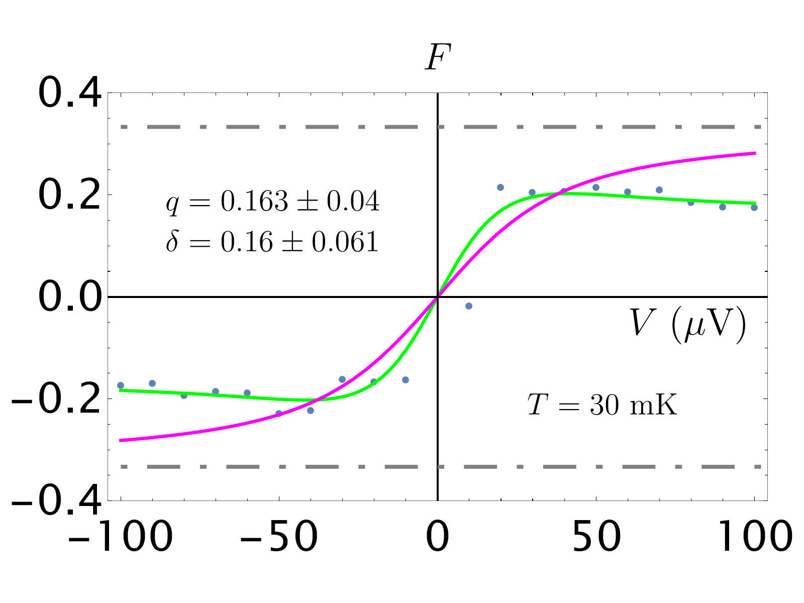
Figure S3 of the supplemental material of Ref. [11] provides the data on the behaviour of two “injection” QPCs used in their “anyonic collider” experiment. The data correspond to the filling factor at temperature and various levels of (8 data sets in total). In Fig. S3, we analyze one representative data set. First note that the standard coth formula (Eq. (5) of the main text) agrees with the data rather loosely — which shows that the standard analysis tolerates rather large errors.555Such tolerance is acceptable when one seeks to establish the existence of fractional quasiparticles, as was originally the aim of such experiments [7, 8]: within such tolerance, is clearly distinct from the characterizing non-interacting electrons. However, this level of tolerance clearly does not enable quantitative characterization of fractionalized excitations. The magnitude of the errors can be seen in the original Figure S3(c) of Ref. [11] — even though the standard way of plotting the noise, and not the Fano factor, makes the errors appear smaller, they are still quite noticeable.
The fit of the same data by the CLL prediction shows the behaviour similar to that discussed in Sec. S2.1 — the fit quality is excellent, the extracted values of are nonsensical. In our view, this is a strong signature of the CLL breakdown taking place. In the code we provide with this paper (https://doi.org/10.5281/zenodo.10840561), we give the reader an opportunity to perform the same analysis of other data sets from Fig. S3 of the supplemental material of Ref. [11].
We next analyse the zero-frequency noise data from Ref. [42]. In this work, the edge mode was part of the edge. Also, the voltage range of the data is much larger than typically used. We analyze the data in Fig. S4. Again, the fit by the CLL prediction is much better that the description by the coth-based phenomenological formula666Interestingly, the deviation from the coth-based prediction for noise is hardly noticeable in Fig. 2(B) of Ref. [42]. The origin of this discrepancy with our plot is unclear to us. It may be another instance when plotting the noise masks the errors that are evident when the Fano factor is considered. and the extracted values of are hardly consistent with the ones expected. Yet, here the fit quality is much lower than what we have seen in Figs. S2 and S3. Noticeably, the Fano factor keeps growing when the saturation is expected both from the CLL fit and the coth formula. The behaviour difference to our data in Fig. S2 and the data of Ref. [11] in Fig. S3 may stem from the fact that here mode of the edge is investigated. Nevertheless, we interpret the results shown in Fig. S4 as a hint that the CLL breakdown happens in this system too.
S3 Energy-dependent scaling dimension renormalization — toy model
Our results in the main text indicate a renormalization of the scaling dimension towards at low energies, with some breakdown of CLL theory at higher energies. Among other features, this results in a deviation from the predicted asymptotic tendency of the Fano factor towards quasiparticle charge at high voltages.
Inspired by these results and by Landauer-Buttiker-Imry scattering theory [63], we present here a toy model of an energy-dependent scaling dimension. We show that a model of this form can recreate qualitative features that we have obtained experimentally. We make no explicit assumption as to the source of this crossover energy scale; however, it has been suggested that the geometry of the QPC, and in particular its width, may affect the tunnelling current [25, 53]. An additional potential energy scale which could be introduced into the system and distinguish high- and low-energy behaviour is the energy associated with Coulomb interactions between the edges.
We begin with the general expressions for the tunnelling current and noise using Landauer-Buttiker-Imry scattering theory. We consider a system of two reservoirs, denoted here by and , with a reflection coefficient of between them. To the leading order in , the tunnelling current and the excess777As in the main text, we define the excess noise as the noise added by a non-zero voltage, rather than as the noise added by the partitioning. tunnelling current noise are given by [63]
| (S4) | ||||
| (S5) |
where is the Fermi-Dirac distribution. Note that we have heuristically replaced the electron charge with the quasiparticle charge, . Also note that corresponds to the noise in a two-terminal QPC experiment, not the 4-terminal one as considered in the rest of the work. This, however, suffices for our purpose in this section, as the expected value of the Fano factor in the 2-terminal experiment is the same. Indeed, when or for and , the dominant contribution to the above integrals comes from the regions where — so, the integrals coincide up to a sign, producing . In what follows, we take and .
Further, energy-dependent can be a toy model for mimicking the CLL behaviour; is a low-energy cutoff (which can be discarded in Eqs. (S4–S5) if ). At for , such produces in agreement with the CLL prediction and , so that .
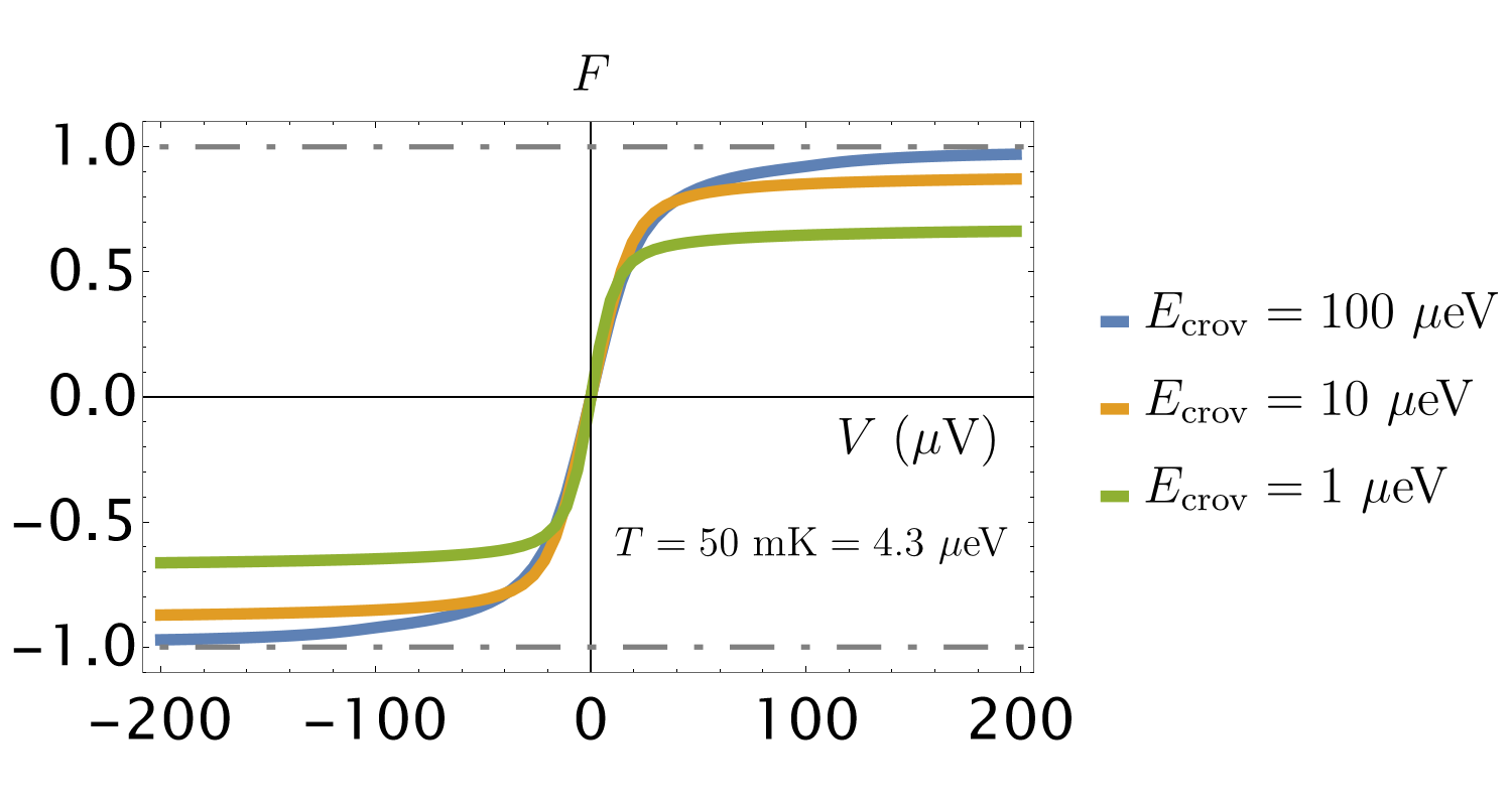
In order to model energy-dependent renormalization of the scaling dimension, we take the transmission coefficient to be
| (S6) |
Here is a crossover energy scale, which separates the low-energy behaviour determined by scaling dimension and the high-energy behaviour determined by scaling dimension .
In Fig. S5, we display how the size of affects the Fano factor. We choose , inspired by the results of the main-text analysis, and , inspired by the theoretically predicted value for the Laughlin state in the absence of renormalization. The value of the charge is chosen to be for convenience. We plot the Fano factor as a function of voltage, with a temperature of .
As can be seen in the figure, the value of greatly affects the asymptotic tendencies of the Fano factor. For , the Fano factor asymptotically tends towards , as predicted by the CLL theory. For smaller , however, the asymptotic value of the Fano factor is significantly reduced.
We emphasize that this is a toy model, and not a proper CLL calculation. However, this toy model demonstrates that energy-dependent renormalization of the scaling dimension may explain the Fano factor’s unexpected behaviour at large .