Abstract

We revisit the problem of offline reinforcement learning with value function realizability but without Bellman completeness. Previous work by Xie and Jiang (2021) and Foster et al. (2022) left open the question whether a bounded concentrability coefficient along with trajectory-based offline data admits a polynomial sample complexity. In this work, we provide a negative answer to this question for the task of offline policy evaluation. In addition to addressing this question, we provide a rather complete picture for offline policy evaluation with only value function realizability. Our primary findings are threefold: 1) The sample complexity of offline policy evaluation is governed by the concentrability coefficient in an aggregated Markov Transition Model jointly determined by the function class and the offline data distribution, rather than that in the original MDP. This unifies and generalizes the ideas of Xie and Jiang (2021) and Foster et al. (2022), 2) The concentrability coefficient in the aggregated Markov Transition Model may grow exponentially with the horizon length, even when the concentrability coefficient in the original MDP is small and the offline data is admissible (i.e., the data distribution equals the occupancy measure of some policy), 3) Under value function realizability, there is a generic reduction that can convert any hard instance with admissible data to a hard instance with trajectory data, implying that trajectory data offers no extra benefits over admissible data. These three pieces jointly resolve the open problem, though each of them could be of independent interest.

1 Introduction

In offline Reinforcement Learning (RL), the learner aims to either find the optimal policy (policy optimization) or evaluate a given policy (policy evaluation) based on pre-collected (offline) data, i.e. without any live interaction with the environment. This approach is relevant in situations where real-time engagement is either impractical or costly, such as in safety-critical applications like healthcare and autonomous driving. The main hurdle in offline RL is the discrepancy between the state-action distribution induced by the given offline data and the target policy, which can significantly compromise our ability to evaluate policies in the environment. Consequently, much of the offline RL research focuses on addressing this data-policy mismatch.

To deal with large state spaces in RL, function approximation is used to generalize the acquired knowledge across states. A key approach in this direction is model-based offline RL, which involves constructing explicit models for transition and reward functions. Theoretical research studies the sample complexity under model realizability, where we assume access to a class that contains the underlying model (Uehara and Sun, 2021). Thus, the sample complexity of model-based offline RL depends on the concentrability coefficient and the model class complexity, where the former quantifies the data-policy distribution mismatch (formally defined in Section 2.2.1) and the latter quantifies the diversity within the model class. Unfortunately, in many tasks, model-based offline RL is not applicable due to the prohibitively large model complexity needed to represent the ground truth model.

Alternatively, value-based offline RL simplifies the process by approximating only the target policy’s value function, typically resulting in lower complexity. Despite being a simpler and more direct approach, achieving polynomial sample complexity under this approach has historically required additional assumptions beyond a bounded concentrability coefficient and value function realizability, such as Bellman completeness (Chen and Jiang, 2019), $\beta$-incompleteness with $\beta<1$ (Zanette, 2023), density-ratio realizability (Xie and Jiang, 2020), pushforward concentrability (Xie and Jiang, 2021), etc. The feasibility of attaining polynomial sample complexity for offline RL with solely bounded concentrability coefficient and realizability remained open for a long time.

The recent work of Foster et al. (2022) provided a negative answer to this question, showing that realizability and concentrability alone cannot ensure polynomial sample complexity in offline RL. Their lower bound construction, however, relies on the offline data being generated somewhat unnaturally—e.g. the offline data includes samples from trajectories that can never be visited by any policy or only includes samples from just the first two steps in an episode, with the later steps hidden from the learner. Thus, the following question remained open:

Is offline RL statistically efficient under value function realizability, bounded concentrability, and natural offline data distribution such as trajectories generated by a single behavior policy?

Our work answers this question in the negative for offline policy evaluation (OPE). Specifically, we show that: There exist MDP instances where even though the offline data consists of trajectories generated by a single behavior policy (used to collect offline data), the value function is realized by a small value function class, action space is finite (binary), and the concentrability coefficient is polynomial in the horizon length, the sample complexity for offline policy evaluation scales exponentially with the horizon.

En route to establishing the above result, we provide a comprehensive characterization for offline policy evaluation with value function approximation and show that to achieve sample efficiency, the concept of “concentrability” needs to be strengthened. In particular, we show that the worst-case sample complexity for offline policy evaluation is both upper and lower bounded via the “aggregated concentrability coefficient” that denotes the data-policy distribution mismatch in an aggregated transition model obtained by clubbing together transitions from the states that have indistinguishable value functions under the given value function class (formally defined in Section 3). On the lower bound side, our results generalize the lower bounds of Foster et al. (2022) since we can show that the aggregated concentrability coefficient is exponentially large in their construction. On the upper bound side, our work recovers the results of Xie and Jiang (2021) since we can show that aggregated concentrability coefficient is upper bounded by the pushforward concentrability coefficient, a notion of data-policy distribution mismatch used in their upper bound.

Having identified that the aggregated concentrability coefficient is the key quantity that governs the sample complexity of offline policy evaluation, we provide a simple example where the offline data distribution is admissible (i.e., the offline data distribution equals the occupancy measure of an offline policy), action space is binary, the standard concentrability coefficient is $O(H^{3})$, but the aggregated concentrability is $2^{\Omega(H)}$, where $H$ is the horizon length. Since aggregated concentrability governs the sample complexity of offline policy evaluation, this implies that realizability, concentrability, and admissibility are not sufficient for sample-efficient OPE.

Finally, to obtain the lower bound for trajectory data, we provide a generic reduction that converts the aforementioned hard instance for admissible data into a hard instance for trajectory data, thus showing that in the worst case, OPE is no easier for trajectory data than for admissible data.

2 Preliminaries

2.1 Markov Decision Process

We consider the finite horizon episodic setting. A Markov Transition Model (MTM), denoted by $M=\textsc{MTM}(\mathcal{X},\mathcal{A},T,H,\rho)$, is parameterized by a state space ${\mathcal{X}}$, an action space ${\mathcal{A}}=\{\mathfrak{a}_{1},\mathfrak{a}_{2},\dots\}$, a transition kernel $T:\mathcal{X}\times\mathcal{A}\mapsto\Delta(\mathcal{X})$, horizon length $H\in\mathbb{N}$, and initial distribution $\rho\in\Delta(\mathcal{X})$. We assume that the state space $\mathcal{X}$ is layered across time, i.e., ${\mathcal{X}}={\mathcal{X}}_{1}\cup{\mathcal{X}}_{2}\cup\dots\cup{\mathcal{X}}_{H}$ with ${\mathcal{X}}_{i}\cap{\mathcal{X}}_{j}=\emptyset$ for any $i\neq j$. The initial distribution $\rho\in\Delta({\mathcal{X}}_{1})$ specifies the state distribution that every episode starts with. The transition kernel $T({x}^{\prime}\mid{}{x},{a})$ for ${x}\in{\mathcal{X}}\setminus{\mathcal{X}}_{H}$, ${x}^{\prime}\in{\mathcal{X}}$ and ${a}\in{\mathcal{A}}$ specifies the probability of transitioning to state ${x}^{\prime}$ if the learner takes action ${a}$ on state ${x}$. Due to the layering structure, $T(\cdot\mid{}{x},{a})$ is supported on ${\mathcal{X}}_{h}$ if ${x}\in{\mathcal{X}}_{h-1}$.

For a MTM $M$ and policy $\pi:{\mathcal{X}}\rightarrow\triangle({\mathcal{A}})$, we let $\mathbb{E}^{M,\pi}[\cdot]$ denote the expectation under the process: ${x}_{1}\sim\rho$, and for $h=1,\ldots,H$, action ${a}_{h}\sim\pi(\cdot\mid{}{x}_{h})$, and next state ${x}_{h+1}\sim T(\cdot\mid{}{x}_{h},{a}_{h})$. Additionally, the state occupancy measure for a particular layer $h$ is defined as $d_{h}^{\pi}({x};M)\vcentcolon={}\mathbb{E}^{M,\pi}[\mathbb{I}\{{x}_{h}={x}\}]$ , and the state-action occupancy measure is defined as $d_{h}^{\pi}({x},{a};M)\vcentcolon={}d_{h}^{\pi}({x};M)\pi({a}\mid{x})$.

A Markov Decision Process (MDP), denoted by $M=\textsc{MDP}({\mathcal{X}},{\mathcal{A}},T,r,H,\rho)$, is a Markov Transition Model augmented with a reward function $r:\mathcal{X}\times\mathcal{A}\to\Delta([-1,1])$. For $h\in[H]$ and policy $\pi$, the state value function $V_{h}^{\pi}(\cdot;M):\mathcal{X}_{h}\mapsto\mathbb{R}$ is defined such that for any $x_{h}\in\mathcal{X}_{h}$, $V_{h}^{\pi}(x_{h};M)$ is the total cumulative reward obtained by starting at state $x_{h}$ at timestep $h$, and acting according to the policy $\pi$ till the end of the episode, i.e. $V_{h}^{\pi}({x};M)=\mathbb{E}^{M,\pi}\big{[}\sum_{k=h}^{H}r({x}_{k},a_{k})\mid{x}_{h}={x}\big{]}$. We similarly define the state-action value function $Q_{h}^{\pi}:\mathcal{X}_{h}\times\mathcal{A}\mapsto\mathbb{R}$ such that for any $x_{h}\in\mathcal{X}_{h}$, $Q_{h}^{\pi}({x},{a})=\mathbb{E}^{M,\pi}[\sum_{h^{\prime}=h}^{H}r({x}_{h^{\prime}},{a}_{h^{\prime}})\mid({x}_{h},{a}_{h})=({x},{a})]$. We let $\Pi$ denote the set of all non-stationary Markovian policies in the underlying MDP.

For the ease of notation, for any policy $\pi$, we define $T({x}^{\prime}\mid{x},\pi)=\mathbb{E}_{{a}\sim\pi(\cdot\mid{x})}[T({x}^{\prime}\mid{x},{a})]$ and $r({x},\pi)=\mathbb{E}_{{a}\sim\pi(\cdot\mid{x})}[r({x},{a})]$, and if $\pi$ is deterministic (i.e., $\pi(\cdot\mid{x})$ is always supported on a single action for every $x\in\mathcal{X}$), we use $\pi({x})\in\mathcal{A}$ to denote the action it chooses on the state ${x}$. Furthermore, whenever clear from the context, we overload the notation and use $r({x},{a})$ to denote the expected value of reward distribution $r({x},{a})$. Furthermore, whenever apparent, we omit the dependency on $M$ and simply write $d_{h}^{\pi}({x}),V_{h}^{\pi}({x})$ and $V^{\pi}(\rho)$, etc. to denote the corresponding occupancy measures and value functions in the MDP $M$.

2.2 Offline RL Preliminaries

Throughout the paper, we consider the offline RL setting. In this setting, the learner is equipped with an offline data distribution $\mu$ and can only gather data about the MDP by i.i.d.  sampling from this offline distribution (however, the learner does not know the density function of $\mu$). We consider three types of offline data models:

1. General Data: The offline dataset is characterized by an offline distribution $\mu=(\mu_{1},\dots,\mu_{H-1})$ where $\mu_{h}\in\Delta(\mathcal{X}_{h}\times\mathcal{A})$ for $h\leq H-1$. An offline sample comprises of $H-1$ many tuples $({x}_{h},{a}_{h},{r}_{h},{x}_{h+1}^{\prime})$, where for each $h\in[H-1]$, $({x}_{h},{a}_{h})\in\mathcal{X}_{h}\times\mathcal{A}$ is drawn from $\mu_{h}$, ${r}_{h}\in[-1,1]$ is drawn from $r({x}_{h},{a}_{h})$, and ${x}_{h+1}^{\prime}\in\mathcal{X}_{h+1}$ is drawn from $T(\cdot\mid{}{x}_{h},{a}_{h})$.

2. Admissible Data: Similar to the General Data setting, but with the addition requirement that there exists an offline policy ${\pi_{b}}\in\Pi$ such that for all ${x}\in\mathcal{X}$ and ${a}\in\mathcal{A}$, $\mu_{h}({x},{a})=d_{h}^{\pi_{b}}({x},{a})$.

3. Trajectory Data: Each offline sample is a complete trajectory $({x}_{1},{a}_{1},{r}_{1},{x}_{2},{a}_{2},{r}_{2},\ldots,$ ${x}_{H})$ sampled in the underlying MDP using an offline policy ${\pi_{b}}$.

The goal of the learner is to estimate the value of a given evaluation policy ${\pi_{\mathrm{e}}}$ by collecting samples from the offline data distribution. In particular, given access to the offline distribution $\mu$, the learner would like to estimate $V^{{\pi_{\mathrm{e}}}}(\rho)$ up to an accuracy of $\varepsilon$, i.e. return a $\widehat{V}$ such that

$$\left\lvert\widehat{V}-V^{{\pi_{\mathrm{e}}}}(\rho)\right\rvert\leq\varepsilon,$$ (1)

where $V^{{\pi_{\mathrm{e}}}}(\rho)=\operatorname{\mathbb{E}}_{x_{1}\sim\rho}\left[V^{{\pi_{\mathrm{e}}}}(x_{1})\right]$. We are interested in quantifying the amount of data required to achieve (1) with high probability. It is not hard to see that learning with general or admissible data is more challenging than learning with trajectory data, because from a trajectory dataset one can generate a $({x},{a},{r},{x}^{\prime})$ dataset with $\mu_{h}({x},{a})=d_{h}^{{\pi_{b}}}({x},{a})$, but not vice versa.

Comparison to the Definition of Admissible Data in Foster et al. (2022).

A result in Foster et al. (2022) also claims to provide an exponential lower bound for admissible data but in the discounted MDP setting. Their data distribution $\mu({x},{a})=\frac{1}{2}(d_{1}^{\pi_{b}}({x},{a})+d_{2}^{\pi_{b}}({x},{a}))$ is not considered as admissible in our definition above. We note that their lower bound construction heavily relies on samples being drawn only from the first two steps, and no information from the third step or later should be revealed. On the other hand, our admissible data definition forces the information to be revealed on all steps. We also remark that our lower bound for our notion of admissible data serves as an important step towards the lower bound for trajectory data (see Section 4.2).

2.2.1 Concentrability Coefficient

Throughout the paper, for simplicity, we consider a fixed and deterministic evaluation policy ${\pi_{\mathrm{e}}}$ that takes the action $\mathfrak{a}_{1}$ on all the states, i.e. ${\pi_{\mathrm{e}}}(x)=\mathfrak{a}_{1}$ for all $x\in\mathcal{X}$. The concentrability coefficient (Munos (2003); Chen and Jiang (2019)) of policy ${\pi_{\mathrm{e}}}$ in an MDP $M=\textsc{MDP}({\mathcal{X}},{\mathcal{A}},T,r,H,\rho)$ with respect to offline data distribution $\mu$ is defined as

$$\mathsf{C}(M,\mu,{\pi_{\mathrm{e}}})=\max_{h}\max_{{x}\in\mathcal{X}_{h},{a}\in\mathcal{A}}\frac{d_{h}^{\pi_{\mathrm{e}}}({x},{a})}{\mu_{h}({x},{a})}.$$ (2)

Whenever clear from the context, we skip ${\pi_{\mathrm{e}}}$ and use the notation $\mathsf{C}(M,\mu)$ to denote $\mathsf{C}(M,\mu,{\pi_{\mathrm{e}}})$.

2.2.2 Function Approximation

The learner is given a function set ${\mathcal{F}}$ that consists of functions of the form ${\mathcal{X}}\times{\mathcal{A}}\rightarrow[-1,1]$. We make the following realizability assumption that the Q-function belongs to the function class $\mathcal{F}$.

Assumption 2.1 (Realizability).

We have $Q^{{\pi_{\mathrm{e}}}}\in\mathcal{F}$.

Given an offline data distribution $\mu$ and a value function class that satisfies realizability, a key question in offline policy evaluation is whether we can design an algorithm that achieves (1), with probability at least $1-\delta$, by only using $\textup{poly}(\log|{\mathcal{F}}|,H,\nicefrac{{1}}{{\delta}},\nicefrac{{1}}{{\varepsilon}},\mathsf{C}(M,\mu))$ offline samples. In the following sections, we argue that this is unfortunately impossible, unless we replace $\mathsf{C}(M,\mu)$ with a different notion of concentrability (see Section 3 for details).

2.2.3 Offline Policy Evaluation Problem

An Offline Policy Evaluation (OPE) problem $\mathfrak{g}$ is given by a tuple $(M,{\pi_{\mathrm{e}}},\mu,\mathcal{F})$ where $M$ denotes the underlying MDP, $\mu$ denotes the offline data distribution, ${\pi_{\mathrm{e}}}$ denotes the evaluation policy, and $\mathcal{F}$ denotes a state-action value function class. Given an OPE instance $\mathfrak{g}$ and a parameter $\varepsilon>0$, the goal of the learner is to estimate the value of the policy ${\pi_{\mathrm{e}}}$ in the MDP $M$ upto precision $\varepsilon$ in expectation, by only relying on samples drawn from the offline distribution $\mu$.

We say that the OPE problem $\mathfrak{g}$ is realizable if $Q^{\pi_{\mathrm{e}}}(\cdot;M)\in\mathcal{F}$. Furthermore, whenever $\mu$ is admissible and there exists a policy ${\pi_{b}}$ such that $\mu_{h}=d_{h}^{\pi_{b}}$ for all $h\leq H$, we often denote the OPE problem as $\mathfrak{g}=(M,{\pi_{\mathrm{e}}},{\pi_{b}},\mathcal{F})$. Finally, in the case of trajectory data, we still use the notation $\mathfrak{g}=(M,{\pi_{\mathrm{e}}},{\pi_{b}},\mathcal{F})$ to denote the OPE problem but explicitly clarify, whenever invoked, that the learner now has access to complete trajectories sampled using ${\pi_{b}}$.

3 State Aggregation in Offline RL

We start by considering the offline policy evaluation problem with general offline data, and introduce useful tools and notation for our main lower bounds for admissible and trajectory data, and our upper bound, in the following sections.

There is a rich literature on understanding the right structural assumptions for offline RL with general offline data. For a warm-up, when the underlying MDP is tabular, i.e. has a small number of states and actions, it is well-known that the concentrability coefficient governs the statistical complexity of offline policy evaluation. To give some intuition for this claim, and to set the foundation for what follows, let $x^{\star}$ denote the state that maximizes the right-hand side in the definition of the concentrability coefficient in (2), and for simplicity, suppose that $d^{\pi_{\mathrm{e}}}(x^{\star})\geq\varepsilon$. Now, consider two scenarios, the first where the MDP has a reward of $+1$ by taking any action in the state $x^{\star}$, and the second where the MDP has a reward of $-1$ by taking any action in $x^{\star}$; in both cases, we assume zero reward on all other states. Thus, to estimate the value of ${\pi_{\mathrm{e}}}$ up to precision $\varepsilon$, the learner needs to distinguish between the two scenarios, and the only way to do so is to observe a transition from $x^{\star}$ in the given offline dataset, which requires at least $\tfrac{1}{\mu({x}^{\star},{\pi_{\mathrm{e}}}({x}^{\star}))}\geq\mathsf{C}$ offline samples from $\mu$, in expectation. To conclude, in tabular MDPs, the learner can explicitly keep track of different states in the MDP, and use the corresponding transition and reward behavior on these states to evaluate ${\pi_{\mathrm{e}}}$, and thus the worst case scenarios for offline policy evaluation is when the offline data does not provide enough information about the parts of the MDP where ${\pi_{\mathrm{e}}}$ has high visitation probability, and thus concentrability coefficient governs the statistical complexity.

The offline policy evaluation problem unfortunately becomes more challenging when the MDP has a large state space and the learner has to rely on function approximation. For this regime, previous works by Xie and Jiang (2021) and Foster et al. (2022) hint that the difficulty of offline policy evaluation comes from the hardness of distinguishing states that have different transition behaviors but the same values. Recall that every piece of data in the offline dataset is of the form $({x},{a},{r},{x}^{\prime})$. If ${x}_{1}$ and ${x}_{2}$ are two states appearing in the dataset such that ${\mathcal{F}}$ does not provide any information to distinguish them, i.e., $f({x}_{1},\cdot)=f({x}_{2},\cdot)$ for all $f\in{\mathcal{F}}$, then the learner has no guidance from ${\mathcal{F}}$ whether they are essentially the same state or not in terms of their rewards or dynamics behavior. There are also no clues from other parts of the dataset, since with high probability, every state only appears at most once in the dataset due to the large state space. Under such a challenging scenario, intuitively, the best the learner can do is to aggregate these two states together and treat them as the same item, to get the most out of the offline dataset and the given value function class. This algorithmic idea of “aggregation” is precisely what is used in the BVFT algorithm of Xie and Jiang (2021). In this following section, we formalize the argument that aggregating indistinguishable states is indeed the best the learner can do by showing a general lower bound in terms of aggregated concentrability coefficient. To establish our lower bound, in the next section, we formally define the notion of state aggregation and aggregated concentrability coefficient.

3.1 Aggregated Concentrability Coefficient

Over a given state space ${\mathcal{X}}={\mathcal{X}}_{1}\cup\dots\cup{\mathcal{X}}_{H}$, we can define a state aggregation scheme $\Phi=\Phi_{1}\cup\dots\cup\Phi_{H}$ as below. For any $h$, $\Phi_{h}$ defines a partition of ${\mathcal{X}}_{h}$ so that the following hold:

1. Every element $\phi\in\Phi_{h}$ is a subset of ${\mathcal{X}}_{h}$;

2. The subsets are disjoint, i.e., $\phi\cap\phi^{\prime}=\emptyset$ for all $\phi,\phi^{\prime}\in\Phi_{h}$;

3. The subsets cover ${\mathcal{X}}_{h}$, i.e., $\bigcup_{\phi\in\Phi_{h}}\phi={\mathcal{X}}_{h}$.

An aggregated Markov Transition Model $\bar{M}$ is defined via a underlying Markov Transition Model $M=({\mathcal{X}},{\mathcal{A}},T,H,\rho)$, state aggregation schemes $\Phi_{h}$, and offline data distributions $\mu_{h}:{\mathcal{X}}_{h}\times{\mathcal{A}}\rightarrow\mathbb{R}_{\geq 0}$ for $1\leq h\leq H-1$. We write $\bar{M}=(M,\Phi,\mu)$. The aggregated transition dynamics for a policy $\pi$ are defined by

$$\bar{T}(\phi^{\prime}\mid{}\phi,\pi;\bar{M})=\frac{\sum_{{x}\in\phi}\sum_{{x}^{\prime}\in\phi^{\prime}}\sum_{{a}\in{\mathcal{A}}}\pi({a}\mid{x})\mu_{h}({x},{a})T({x}^{\prime}\mid{}{x},{a})}{\sum_{{x}\in\phi}\sum_{{a}\in{\mathcal{A}}}\pi({a}\mid{x})\mu_{h}({x},{a})}$$ (3)

for $\phi\in\Phi_{h}$, $\phi^{\prime}\in\Phi_{h+1}$. The aggregated occupancy measure for a policy $\pi$ is defined as

$$\bar{d}_{h}^{\pi}(\phi;\bar{M})\vcentcolon={}\mathbb{E}\left[\mathbb{I}\{\phi_{h}=\phi\}\leavevmode\nobreak\ \bigg{|}\leavevmode\nobreak\ \phi_{1}\sim\bar{\rho}(\cdot),\phi_{i+1}\sim\bar{T}(\cdot\mid{}\phi_{i},\pi;\bar{M}),\forall 1\leq i\leq h-1\right],$$

where the initial distribution $\bar{\rho}$ is defined as $\bar{\rho}(\phi)\vcentcolon={}\sum_{{x}\in\phi}\rho({x})$.

Note that in general, it may not be meaningful to define aggregated transitions with respect to actions, i.e., $\bar{T}(\phi^{\prime}\mid\phi,{a};\bar{M})$. This is because states in the same aggregation may not even share the same action space. However, in the special case where states within the same aggregation share the same action space, the quantity $\bar{T}(\phi^{\prime}\mid\phi,{a};\bar{M})$ can be defined, which could be useful in simplifying the notation. We use this notation in our lower bound proof (Appendix C).

Definition 3.1 (Aggregated Concentrability Coefficient).

For an aggregated MDP $\bar{M}=(M,\Phi,\mu)$ with underlying MDP $M$, aggregation scheme $\Phi$, and offline distribution $\mu$, we define the aggregated concentrability coefficient $\bar{\mathsf{C}}_{\varepsilon}(M,\Phi,\mu)$ as

$$\bar{\mathsf{C}}_{\varepsilon}(M,\Phi,\mu)=\max_{h}\max_{\mathcal{I}}\left\{\frac{\sum_{\phi\in\mathcal{I}}\bar{d}_{h}^{\pi_{\mathrm{e}}}(\phi)}{\sum_{\phi\in\mathcal{I}}\sum_{{x}\in\phi}\mu_{h}({x},{\pi_{\mathrm{e}}}({x}))}\leavevmode\nobreak\ \leavevmode\nobreak\ \Bigg{|}\leavevmode\nobreak\ \leavevmode\nobreak\ {\mathcal{I}}\subseteq\Phi_{h},\ \ \sum_{\phi\in{\mathcal{I}}}\bar{d}_{h}^{\pi_{\mathrm{e}}}(\phi)\geq\varepsilon\right\}.$$

The aggregated concentrability coefficient is analogous to the standard concentrability coefficient defined in (2), but now under the aggregated transition model. The reason why the sum of aggregated occupancy measure is restricted to be at least $\varepsilon$ above is because those $\phi$ with extremely small occupancy can be fully ignored during the policy evaluation process, while making no impact in the estimation error even if the above ratio is large.

3.2 A General Lower Bound in Terms of Aggregated Concentrability Coefficient

We now have all the necessary tools to state our first lower bound. The following theorem provides a general reduction that lifts any given instance of a Markov Transition Model, evaluation policy, offline data distribution, and aggregation scheme into a class of offline policy evaluation problems, and provides a statistical lower bound for offline policy evaluation for this class in terms of the aggregated concentrability coefficient.

Theorem 3.1.

Let $\varepsilon\in(0,1)$, $M$ be a Markov Transition Model, $\Phi$ be an aggregation scheme over the states of $M$, ${\pi_{\mathrm{e}}}$ be a deterministic evaluation policy in $M$ such that for any aggregation $\phi\in\Phi$ and states $x,x^{\prime}\in\phi$ it holds that ${\pi_{\mathrm{e}}}(x)={\pi_{\mathrm{e}}}(x^{\prime})$, and $\mu$ be a general offline data distribution with standard concentrability coefficient $\mathsf{C}(M,\mu)$ and aggregated concentrability coefficient $\bar{\mathsf{C}}_{\varepsilon}(M,\Phi,\mu)$. Then, there exists a class $\mathfrak{G}$ of realizable OPE problems such that for every OPE problem $\mathfrak{g}=\textsc{OPE}\left(M^{\scriptscriptstyle(\mathfrak{g})},{\pi_{\mathrm{e}}}^{\scriptscriptstyle(\mathfrak{g})},\mu^{\scriptscriptstyle(\mathfrak{g})},\mathcal{F}^{\scriptscriptstyle(\mathfrak{g})}\right)$ in $\mathfrak{G}$,

1. The function class $\mathcal{F}^{\scriptscriptstyle(\mathfrak{g})}$ satisfies $Q^{{\pi_{\mathrm{e}}}}(\cdot;M^{\scriptscriptstyle(\mathfrak{g})})\in\mathcal{F}^{\scriptscriptstyle(\mathfrak{g})}$ (Assumption 2.1), and $\lvert\mathcal{F}^{\scriptscriptstyle(\mathfrak{g})}\rvert=2$.

2. Any pair of states $x,x^{\prime}$ that belong to the same aggregation $\phi\in\Phi$ satisfy $f(x,\cdot)=f(x^{\prime},\cdot)$ for all $f\in\mathcal{F}^{\scriptscriptstyle(g)}$.

3. The concentrability coefficient $\mathsf{C}(M^{\scriptscriptstyle(\mathfrak{g})},\mu^{\scriptscriptstyle(\mathfrak{g})})=\Theta(\mathsf{C}(M,\mu))$.

Furthermore, any offline policy evaluation algorithm that guarantees to estimate the value of ${\pi_{\mathrm{e}}}^{\scriptscriptstyle(\mathfrak{g})}$ in the MDP $M^{\scriptscriptstyle(\mathfrak{g})}$ up to precision $\varepsilon$, in expectation, for every OPE problem $\mathfrak{g}\in\mathfrak{G}$ must use

$$\widetilde{\Omega}\left(\frac{\bar{\mathsf{C}}_{\varepsilon}(M,\Phi,\mu)}{\varepsilon}\right)$$

offline samples from $\mu^{\scriptscriptstyle(\mathfrak{g})}$ in some OPE problem $\mathfrak{g}\in\mathfrak{G}$.

The proof of Theorem 3.1 is deferred to Appendix C. In the proof, instead of directly using the given MTM $M$ to construct the class $\mathfrak{G}$, we construct Block MDPs $\{M^{\scriptscriptstyle(\mathfrak{g})}\}_{\mathfrak{g}\in\mathfrak{G}}$ with latent state dynamics given by $M$ (with three additional new latent states per layer). As shown in the appendix, this reduction ensures that the standard concentrability remains unchanged. Furthermore, we note that the function class $\mathcal{F}^{\scriptscriptstyle(\mathfrak{g})}$ and the evaluation policy ${\pi_{\mathrm{e}}}^{\scriptscriptstyle(\mathfrak{g})}$ are the same for all instances $\mathfrak{g}\in\mathcal{G}$, and that the aggregated concentrability coefficient in $M^{\scriptscriptstyle(g)}$ is $\Theta(\bar{\mathsf{C}}_{\varepsilon}(M,\Phi,\mu))$ (see Proposition 2). We also have the following property.

Property 1.

In the construction in Theorem 3.1, if the offline distribution $\mu$ is admissible for the Markov Transition Model $M$, then for every OPE problem $\mathfrak{g}\in\mathfrak{G}$, the offline distribution $\mu^{\scriptscriptstyle(\mathfrak{g})}$ is also admissible for the corresponding MDP $M^{\scriptscriptstyle(\mathfrak{g})}$.

3.3 Can Aggregated Concentrability be Larger than Standard Concentrability?

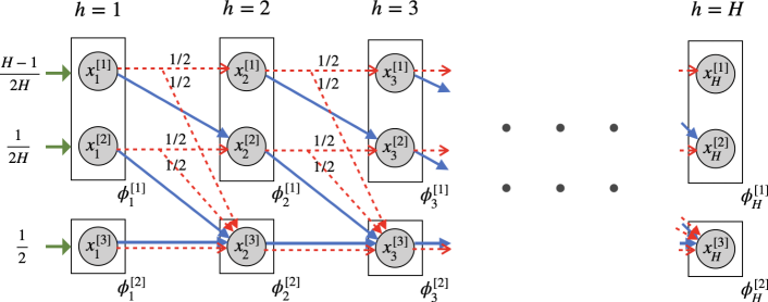
Figure 1: Markov Transition Model and aggregation scheme in Example 1. The blue arrows represent the transitions under action $\mathfrak{a}_{1}$, and the red arrows represent the transitions under $\mathfrak{a}_{2}$. The green arrows denote the initial distribution $\rho$.

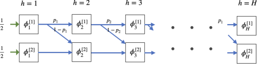
Figure 2: Dynamics for policy ${\pi_{\mathrm{e}}}$ in the aggregated MDP $\bar{M}$ in Example 1, where $p_{h}\vcentcolon={}\bar{T}\left(\phi_{h+1}^{\scriptscriptstyle[1]}\mid\phi_{h}^{\scriptscriptstyle[1]},{\pi_{\mathrm{e}}};\bar{M}\right)$. As shown in Lemma 17, $p_{h}\geq\frac{H-1}{H+2}$ for all $1\leq h\leq H-1$. The green arrows denote the initial distribution $\rho$ in the aggregated MDP.

Theorem 3.1 indicates that the sample complexity of offline policy evaluation (with general data) grows with the aggregated concentrability coefficient $\bar{\mathsf{C}}_{\varepsilon}(M,\Phi,\mu)$ instead of the standard concentrability coefficient $\mathsf{C}(M,\mu)$. Given this lower bound, one may wonder how large can the aggregated concentrability be in comparison to the standard concentrability. In this section, we will demonstrate via an example that the gap could indeed be exponential.

Example 1.

Consider the example represented in Figure 1, where

1. Markov Transition Model $M$ consists of three states $\{x_{h}^{\scriptscriptstyle[1]},x_{h}^{\scriptscriptstyle[2]},x_{h}^{\scriptscriptstyle[3]}\}$ in each layer $h\in[H]$, and two actions $\mathcal{A}=\{\mathfrak{a}_{1},\mathfrak{a}_{2}\}$. The initial distribution $\rho$ (denoted by the solid green arrows) is defined such that $\rho\left(x_{1}^{\scriptscriptstyle[1]}\right)=\nicefrac{{(H-1)}}{{2H}}$, $\rho\left(x_{1}^{\scriptscriptstyle[2]}\right)=\nicefrac{{1}}{{2H}}$ and $\rho\left(x_{1}^{\scriptscriptstyle[3]}\right)=\nicefrac{{1}}{{2}}$.

   The transition dynamics are identical for every layer $h\in[H-1]$, and is defined such that on taking action $\mathfrak{a}_{1}$ the agent transitions deterministically according to the solid blue arrows, and on taking action $\mathfrak{a}_{2}$, the agent transitions stochastically according to the dotted red arrows.

2. For every $h\in[H]$, the aggregation scheme $\Phi_{h}=\{\phi_{h}^{\scriptscriptstyle[1]},\phi_{h}^{\scriptscriptstyle[2]}\}$ with the aggregation $\Phi_{h}^{\scriptscriptstyle[1]}=\{x_{h}^{\scriptscriptstyle[1]},x_{h}^{\scriptscriptstyle[2]}\}$ and $\phi_{h}^{\scriptscriptstyle[2]}=\{x_{h}^{\scriptscriptstyle[3]}\}$. The aggregated states are denoted by rectangular blocks.

3. The offline distribution $\mu$ is the occupancy measure of an offline policy ${\pi_{b}}$ defined such that ${\pi_{b}}(x)=\frac{1}{H^{2}}\delta_{\mathfrak{a}_{1}}(\cdot)+\frac{H^{2}-1}{H^{2}}\delta_{\mathfrak{a}_{2}}(\cdot)$ for all $x\in\mathcal{X}$

4. The evaluation policy ${\pi_{\mathrm{e}}}$ such that ${\pi_{\mathrm{e}}}(x)=\delta(\mathfrak{a}_{1})$ for all $x\in\mathcal{X}$.

Proposition 1.

For $\varepsilon\leq\nicefrac{{1}}{{15}}$, the Markov Transition Model $M$, aggregation scheme $\Phi$, evaluation policy ${\pi_{\mathrm{e}}}$ and offline distribution $\mu$ given in Example 1, the standard concentrability coefficient $\mathsf{C}(M,\mu)=O(H^{3})$, whereas the aggregated concentrability coefficient $\bar{\mathsf{C}}_{\varepsilon}(M,\Phi,\mu)=\widetilde{\Omega}(2^{H})$.

We now give a sketch for the proof of Proposition 1, with the full details deferred to Appendix D. We first calculate the upper bound on the standard concentrability coefficient. First, we argue that for $h\geq 3$, $d^{{\pi_{\mathrm{e}}}}_{h}({x}_{h})=1$ if ${x}_{h}={x}_{h}^{\scriptscriptstyle[3]}$ and $0$ otherwise. This can be easily observed from the transition of ${\pi_{\mathrm{e}}}$ (blue arrow) in Figure 1—following the blue arrow, the policy must stay in ${x}_{h}^{\scriptscriptstyle[3]}$ for $h\geq 3$. Next, we lower bound the state occupancy under ${\pi_{b}}$. We claim that

$$d_{h}^{{\pi_{b}}}\left({x}_{h}^{\scriptscriptstyle[1]}\right)\geq\Omega\left(\frac{1}{2^{h}}\right),\quad d_{h}^{{\pi_{b}}}\left({x}_{h}^{\scriptscriptstyle[2]}\right)\geq\Omega\left(\frac{1}{H2^{h}}\right),\leavevmode\nobreak\ \quad\text{\ and\ }\quad d_{h}^{{\pi_{b}}}\left({x}_{h}^{\scriptscriptstyle[3]}\right)\geq\frac{1}{2}.$$ (4)

The third inequality in (4) is easy to see since the occupancy on ${x}_{h}^{\scriptscriptstyle[3]}$ is non-decreasing w.r.t. $h$ under any policy (Figure 1). To see the first two inequalities in (4), notice that since ${\pi_{b}}$ chooses $\mathfrak{a}_{2}$ with probability $1-\frac{1}{H^{2}}$, and $\mathfrak{a}_{2}$ carries $\frac{1}{2}$ of the weights from ${x}_{h}^{\scriptscriptstyle[1]}$ to ${x}_{h+1}^{\scriptscriptstyle[1]}$ (depicted by the red arrow in Figure 1), we have $d_{h}^{{\pi_{b}}}({x}_{h}^{{}^{\scriptscriptstyle[1]}})\geq\rho({x}_{1}^{{}^{\scriptscriptstyle[1]}})\left(\frac{1}{2}(1-\frac{1}{H^{2}})\right)^{h-1}=\Omega\left(\frac{1}{2^{h}}\right)$. Similarly, $d_{h}^{{\pi_{b}}}({x}_{h}^{{}^{\scriptscriptstyle[2]}})\geq\rho({x}_{1}^{{}^{\scriptscriptstyle[2]}})\left(\frac{1}{2}(1-\frac{1}{H^{2}})\right)^{h-1}=\Omega\left(\frac{1}{H2^{h}}\right)$. With the above calculation and that $\tfrac{{\pi_{\mathrm{e}}}({a}|{x})}{{\pi_{b}}({a}|{x})}\leq H^{2}$, we conclude that $\mathsf{C}\leq H^{2}\max_{h}\max_{{x}}\tfrac{d_{h}^{{\pi_{\mathrm{e}}}}({x})}{d_{h}^{{\pi_{b}}}({x})}\leq O(H^{3})$.

We now proceed to the lower bound on aggregated concentrability coefficient. From (3), we know that the aggregated dynamic for ${\pi_{\mathrm{e}}}$, shown in Figure 2, is constructed by reweighting the transition in the original transition model using $\mu_{h}(\cdot)=d_{h}^{\pi_{b}}(\cdot)$. Since ${\pi_{b}}$ takes action $\mathfrak{a}_{2}$ with large probability, and $\mathfrak{a}_{2}$ does not change the relative weight $\tfrac{d_{h}^{\pi_{b}}(x_{h}^{\scriptscriptstyle[1]})}{d_{h}^{\pi_{b}}(x_{h}^{\scriptscriptstyle[2]})}$ (see the red arrows in Figure 1), it can be shown that $\tfrac{d_{h}^{\pi_{b}}(x_{h}^{\scriptscriptstyle[1]})}{d_{h}^{\pi_{b}}(x_{h}^{\scriptscriptstyle[2]})}\geq\tfrac{\rho(x_{1}^{\scriptscriptstyle[1]})}{3\rho(x_{1}^{\scriptscriptstyle[2]})}=\tfrac{H-1}{3}$ for all $h$. This gives

$$p_{h}\vcentcolon={}\bar{T}(\phi_{h+1}^{\scriptscriptstyle[1]}\mid\phi_{h}^{\scriptscriptstyle[1]},{\pi_{\mathrm{e}}})=\frac{d_{h}^{\pi_{b}}(x_{h}^{\scriptscriptstyle[1]})\cdot 1+d_{h}^{\pi_{b}}(x_{h}^{\scriptscriptstyle[2]})\cdot(\nicefrac{{1}}{{2}})}{d_{h}^{\pi_{b}}(x_{h}^{\scriptscriptstyle[1]})+d_{h}^{\pi_{b}}(x_{h}^{\scriptscriptstyle[2]})}\geq\frac{H-1}{H+2},$$

where the factors of $1$ and $\nicefrac{{1}}{{2}}$ are the probability of transitioning to $\phi_{h+1}^{\scriptscriptstyle[1]}$ from ${x}_{h}^{\scriptscriptstyle[1]}$ and ${x}_{h}^{\scriptscriptstyle[2]}$ following ${\pi_{\mathrm{e}}}$. This further implies $\bar{d}_{h}^{\pi_{\mathrm{e}}}(\phi_{h}^{\scriptscriptstyle[1]})\geq\frac{1}{2}\left(\frac{H-1}{H+2}\right)^{h}$. Using a similar argument as for (4), we have $\bar{d}_{h}^{\pi_{b}}(\phi_{h}^{\scriptscriptstyle[1]})\leq\tfrac{1}{2^{h}}$. These two bounds together imply that the aggregated concentrability is $2^{\Omega(H)}$.

4 Main Lower Bounds for Offline Policy Evaluation

4.1 Admissible Data

Example 1 provides an instance of a Markov Transition Model, aggregation scheme, evaluation policy and offline distribution for which the standard concentrability is $O(H^{3})$ whereas the aggregated concentrated is $2^{\Omega(H)}$. Since the offline distribution $\mu$ in Example 1 is the occupancy measure $d^{\pi_{b}}$ for the policy ${\pi_{b}}$, plugging Example 1 in Theorem 3.1 implies the following lower bound for offline policy evaluation with admissible offline data.

Theorem 4.1.

Let $\varepsilon\leq\nicefrac{{1}}{{15}}$, and horizon $H\geq 1$. Then, there exits a class $\mathfrak{G}_{\textsc{adm}}$ of realizable OPE problems, such that for every OPE problem $\mathfrak{g}=\left(M^{\scriptscriptstyle(\mathfrak{g})},{\pi_{\mathrm{e}}}^{\scriptscriptstyle(\mathfrak{g})},\mu^{\scriptscriptstyle(\mathfrak{g})},\mathcal{F}^{\scriptscriptstyle(\mathfrak{g})}\right)\in\mathfrak{G}_{\textsc{adm}}$, the concentrability coefficient of ${\pi_{\mathrm{e}}}^{\scriptscriptstyle(\mathfrak{g})}$ w.r.t.  $\mu^{\scriptscriptstyle(\mathfrak{g})}$ is $O(H^{3})$, the offline distribution $\mu^{\scriptscriptstyle(\mathfrak{g})}$ is admissible for the MDP $M^{\scriptscriptstyle(\mathfrak{g})}$, and $\lvert\mathcal{F}^{\scriptscriptstyle(\mathfrak{g})}\rvert=2$.

Furthermore, any offline policy evaluation algorithm that guarantees to estimate the value of ${\pi_{\mathrm{e}}}^{\scriptscriptstyle(\mathfrak{g})}$ in the MDP $M^{\scriptscriptstyle(\mathfrak{g})}$ up to precision $\varepsilon$, in expectation, for every OPE problem $\mathfrak{g}\in\mathfrak{G}_{\textsc{adm}}$ must use $2^{\Omega(H)}$ offline samples in some $\mathfrak{g}\in\mathfrak{G}_{\textsc{adm}}$.

The construction of the class $\mathfrak{G}_{\textsc{adm}}$, and the proof of Theorem 4.1, are deferred to Appendix D. We remark that in all the OPE problem instances $\mathfrak{g}\in\mathfrak{G}_{\textsc{adm}}$, the corresponding MDPs $M^{\scriptscriptstyle(\mathfrak{g})}$ share the same action space $\mathcal{A}=\{a_{1},a_{2}\}$ (binary actions), state space $\mathcal{X}$ and horizon $H$, however, the transition dynamics, reward function and initial distribution could change with the instance. Furthermore, the policy ${\pi_{\mathrm{e}}}^{\scriptscriptstyle(\mathfrak{g})}$ and the state-action value function class $\mathcal{F}^{\scriptscriptstyle(\mathfrak{g})}$ are also same across all instances $\mathfrak{g}\in\mathfrak{G}_{\textsc{adm}}$.

Our lower bound in Theorem 4.1 considers admissible offline data distributions, where for any instance $\mathfrak{g}\in\mathfrak{G}_{\textsc{adm}}$ and $h\leq H$, the offline distribution $\mu_{h}^{\scriptscriptstyle(\mathfrak{g})}=d_{h}^{{\pi_{b}}^{\scriptscriptstyle(\mathfrak{g})}}(\cdot;M^{\scriptscriptstyle(\mathfrak{g})})$, and the offline algorithm can draw samples of the form $(x_{h},a_{h},r_{h},x_{h+1})$ from the process $(x_{h},a_{h})\sim\mu_{h}^{\scriptscriptstyle(\mathfrak{g})}$, $r_{h}\sim r^{\scriptscriptstyle(\mathfrak{g})}(x_{h},a_{h})$ and $x_{h+1}\sim T^{\scriptscriptstyle(\mathfrak{g})}(\cdot\mid x_{h},a_{h})$. Thus, Theorem 4.1 strengthens over the results of Foster et al. (2022), in which the offline data distribution is not equal to the occupancy measure of a single policy.

Having shown that bounded concentrability coefficient and realizability alone are not sufficient for statistically efficient offline policy evaluation, even if the offline distribution $\mu_{h}=d^{{\pi_{b}}}_{h}$ is admissible, we now ask what happens if the learner has access to complete offline trajectories $(x_{1},a_{1},r_{1},s_{2},\dots,r_{H},s_{H})$ sampled using ${\pi_{b}}$. Unfortunately, for this scenario, the result of Theorem 4.1 no longer holds. This is because the reduction in Theorem 3.1, which is a key tool in the proof of Theorem 4.1, does not prevent from leaking additional information when the learner has access to trajectories of length more than $2$. In particular, by looking at the conditional distributions of $x_{3}$ after fixing actions $a_{1}$ and $a_{2}$ for the first two timesteps in that construction (which can be computed when given trajectory data that covers the first two timesteps), the learner can infer the value of ${\pi_{\mathrm{e}}}$ in the underlying MDP. In the next section, we develop additional tools to handle trajectory data.

4.2 Trajectory Data

In many real world applications, the offline dataset is collected by sampling trajectories of the form $({x}_{1},{a}_{1},{r}_{1},{x}_{2},\dots,{x}_{H},{a}_{H},{r}_{H})$ and it remains to address whether access to the entire $H$-length trajectory instead of just the tuples $({x},{a},{r},{x}^{\prime})$ can allow the learner to circumvent the challenges introduced in previous subsections. In fact, Foster et al. (2022) left it as an open problem whether access to trajectory data can make offline RL statistically tractable. In this section, we answer this in the negative and show that in the worst case, access to trajectory data does not overcome the statistical inefficiencies of offline RL with just bounded concentrability coefficient and realizability.

Theorem 4.2.

Let $\varepsilon\leq\nicefrac{{1}}{{15}}$, and horizon $H\geq 1$. Then, there exits a class $\mathfrak{G}_{\textsc{traj}}$ of realizable OPE problems, such that for every OPE problem $\mathfrak{g}=\left(M^{\scriptscriptstyle(\mathfrak{g})},{\pi_{\mathrm{e}}}^{\scriptscriptstyle(\mathfrak{g})},{\pi_{b}}^{\scriptscriptstyle(\mathfrak{g})},\mathcal{F}^{\scriptscriptstyle(\mathfrak{g})}\right)\in\mathfrak{G}_{\textsc{traj}}$, the learner has access to offline trajectories sampled using ${\pi_{b}}^{\scriptscriptstyle(\mathfrak{g})}$, the concentrability coefficient of ${\pi_{\mathrm{e}}}^{\scriptscriptstyle(\mathfrak{g})}$ w.r.t.  ${\pi_{b}}^{\scriptscriptstyle(\mathfrak{g})}$ is $O(H^{3})$, and $\lvert\mathcal{F}^{\scriptscriptstyle(\mathfrak{g})}\rvert=2$.

Furthermore, any offline policy evaluation algorithm that estimates the value of ${\pi_{\mathrm{e}}}^{\scriptscriptstyle(\mathfrak{g})}$ in the MDP $M^{\scriptscriptstyle(\mathfrak{g})}$ up to precision $\varepsilon/(16H)$, in expectation, for every OPE problem $\mathfrak{g}\in\mathfrak{G}_{\textsc{traj}}$ must use $2^{\Omega(H)}$ offline trajectories in some $\mathfrak{g}\in\mathfrak{G}_{\textsc{traj}}$.

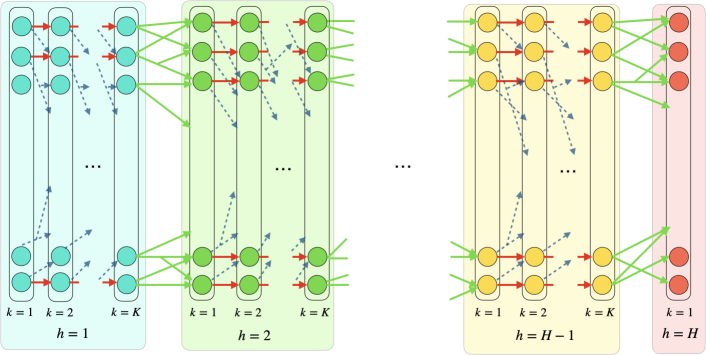
Figure 3: Lower bound construction for the proof of Theorem G.1. For each $h\in[H]$, the corresponding block denotes the $K$ layers that are obtained using Replicator by replicating the $h$-th layer in the given MDP $M$ for $K$ many times. The solid red arrows represent the transitions under the action $\mathfrak{a}_{1}$, the dotted blue arrows represent the transitions under the $\mathfrak{a}_{2}$ (under which we resample from the admissible distribution $\mu_{h}$), the solid green arrows denote the transitions according to the original MDP $M$.

While the full proof is deferred to Appendix E, we present the main ideas and the key tools below. The primary reason why the lower bound from Theorem 4.1 does not hold under trajectory data is that access to trajectories spanning more than two timesteps in the underlying MDPs in that construction leaks additional information, which can be exploited by the learner to evaluate ${\pi_{\mathrm{e}}}$. In particular, given trajectory data, the learner can compute the marginal distribution over $x_{h+2}$ given actions $a_{h}$ and $a_{h+1}$, for $h\leq H-2$, which can be used to identify the underlying instance in the class $\mathfrak{G}_{\textsc{adm}}$ and thus compute ${\pi_{\mathrm{e}}}$. Our key insight in the proof is to fix this problem of information leakage by introducing a general-purpose reduction from offline RL with admissible data to offline RL with trajectory data, which may be of independent interest. This reduction is obtained by using two new protocols called (a) the Replicator protocol, and (b) the admissible-to-trajectory protocol, which we describe below.

Replicator:

Given in Algorithm 1 in the appendix, the Replicator protocol takes as input a realizable OPE problem $\mathfrak{g}=(M,{\pi_{b}},{\pi_{\mathrm{e}}},\mathcal{F})$ where the MDP $M$ has horizon $H$, and a parameter $K$, and converts it into another realizable OPE problem $\widetilde{\mathfrak{g}}=(\widetilde{M},\widetilde{{\pi_{b}}},{{\widetilde{\pi}}_{\mathrm{e}}},\mathcal{F})$ where the new MDP $\widetilde{M}$ has horizon $\widetilde{H}=(H-1)K+1$. We require that Replicator satisfies the following property.

Property 2 (Informal; Formal version in Lemma 20).

The realizable OPE problem $\widetilde{\mathfrak{g}}\leftarrow\textsc{Replicator}(\mathfrak{g},K)$ satisfies the following:

1. Concentrability coefficient $\sup_{\widetilde{h}\leq\widetilde{H}}\left\|\frac{d_{h}^{{{\widetilde{\pi}}_{\mathrm{e}}}}}{d_{h}^{\widetilde{{\pi_{b}}}}}\right\|_{\infty}\leq 2\sup_{h\leq H}\left\|\frac{d_{h}^{{\pi_{\mathrm{e}}}}}{d_{h}^{\pi_{b}}}\right\|_{\infty}.$

2. The value of the policy ${{\widetilde{\pi}}_{\mathrm{e}}}$ in $\widetilde{M}$ is equal to the value of ${\pi_{\mathrm{e}}}$ in $M$.

Our construction of Replicator essentially replicates each layer in the given MDP $M$ for $K$ times (except for the last layer); see Figure 3 for illustration. In the following, we call these replicated layers as sub-layers. We first define the transition function. For the last sub-layer (i.e., for $k=K$) of each layer $h\leq H-1$, the transition is exactly the same as that in the MDP from layer $h$ to $h+1$ (denoted by the green arrows in Figure 3). For other sublayers with $k<K$, the transitions are designed such that: if the action $\mathfrak{a}_{1}$ is taken, then the state transitions to the same state in the next sub-layer (red arrows in Figure 3); and if the action $\mathfrak{a}_{2}$ is taken, the next state is sampled independently from the offline data distribution $\mu_{h}=d^{\pi_{b}}_{h}$ (blue arrows in Figure 3). Furthermore, the evaluation policy ${{\widetilde{\pi}}_{\mathrm{e}}}$ in the new MDP is the same as ${\pi_{\mathrm{e}}}$, and takes action $\mathfrak{a}_{1}$ on all states. The offline policy $\widetilde{{\pi_{b}}}$ is set as ${\pi_{b}}$ for the last sub-layer (i.e. $k=K$), and is set as $\frac{1}{2}\left(\delta_{\mathfrak{a}_{1}}+\delta_{\mathfrak{a}_{2}}\right)$ for the intermediate sub-layers with $k\leq K-1$.

The rationale behind this design is that since $\widetilde{{\pi_{b}}}=\frac{1}{2}\left(\delta_{\mathfrak{a}_{1}}+\delta_{\mathfrak{a}_{2}}\right)$, for each $h$, with probability $1-2^{-K+1}$ the offline policy will choose $\mathfrak{a}_{2}$ at least once in sub-layers $k=1,\ldots,K-1$. If $\mathfrak{a}_{2}$ is chosen at least once, then the state distribution at $k=K$ is equal to $\mu_{h}=d^{{\pi_{b}}}$ and independent from all previous layers $1,\ldots,h-1$. As long as $K$ is large enough, this happens with very high probability, which makes the offline data distribution at sub-layer $k=K$ resemble admissible data with distribution $\mu_{h}=d^{{\pi_{b}}}_{h}$, even when the data is actually a complete trajectory. It can be shown that this conversion preserves the concentrability coefficient up to a constant factor.

admissible-to-trajectory:

Given in Algorithm 2 in the appendix, this protocol takes as input $K$ tuples of the form $({x}_{h},{a}_{h},{r}_{h},{x}_{h+1})$ sampled from an admissible offline distribution $\mu_{h}=d_{h}^{{\pi_{b}}}$, for every $h\in[H]$, and returns a trajectory $\widetilde{\tau}$ of length $\widetilde{H}$ in $\widetilde{M}$. We require that admissible-to-trajectory satisfies the following property.

Property 3 (Informal; Formal version in Lemma 21).

For a large class of offline policies ${\pi_{b}}$, the distribution of trajectory $\widetilde{\tau}$, constructed by admissible-to-trajectory using offline data tuples from $d^{\pi_{b}}$, is close to the distribution of trajectories $\widetilde{\tau}^{\prime}$ obtained using $\widetilde{{\pi_{b}}}$ in $\widetilde{M}$.

The idea of admissible-to-trajectory is straightforward: We already argue that Replicator can simulate admissible data using trajectory data. Hence, with a reverse process, given an admissible dataset, we can create a new trajectory dataset in a new MDP that simulates the original admissible dataset.

With the above two protocols, the reduction of offline RL with admissible data to trajectory data is straightforward and is stated in Algorithm 3 in the appendix. At a high level, given a realizable OPE problem $g$ with admissible offline distribution $d^{{\pi_{b}}}$, for some large enough $K$, we use the Replicator protocol to create a realizable OPE problem $\widetilde{g}$ and use the admissible-to-trajectory protocol to generate trajectory data corresponding to $\widetilde{{\pi_{b}}}$ in $\widetilde{M}$. Since, Property 2-(a) implies that the concentrability coefficient stays bounded and Property 2-(b) implies that the value to be evaluated remains unchanged, the above reduction provides a way to solve offline RL with admissible data by invoking an offline algorithm that requires trajectory data. Thus, if trajectory data with bounded concentrability coefficient is tractable, then so is admissible data by leveraging Algorithm 3, which contradicts Theorem 4.1. This implies that offline RL with trajectory data must also be statistically inefficient. The formal proof is deferred to Appendix E.

5 Upper Bound

Our lower bounds show that the worst-case sample complexity of offline policy evaluation grows with the aggregated concentrability. In this section, we complement our lower bounds with an upper bound of the form $\textup{poly}(\bar{\mathsf{C}},H,\varepsilon^{-1},\log|{\mathcal{F}}|)$. Taken together, the lower and upper bound suggest that aggregated concentrability, but not the standard concentrability, characterize the worst-case sample complexity of offline policy evaluation with value function approximation.

Theorem 5.1.

Let $\varepsilon>0$, $\mathcal{F}$ be a state-action value function class that satisfies Assumption 2.1, ${\pi_{\mathrm{e}}}$ be an evaluation policy and $\mu$ be an offline (general) data distribution. Then, Algorithm 4 (a adaptation of the BVFT algorithm of Xie and Jiang (2021)) returns a $\widehat{V}$ such that $\left\lvert\mathbb{E}_{{x}\sim\rho}[V^{\pi_{\mathrm{e}}}({x})-\widehat{V}]\right\rvert=O\left(\varepsilon\right)$ after collecting

$$n=\mathcal{O}\left(\frac{\bar{\mathsf{C}}\cdot H^{6}\log(|{\mathcal{F}}|/\delta)}{\varepsilon^{4}}\right)$$

many (offline) samples from $\mu$, where $\bar{\mathsf{C}}:=\max_{f,f^{\prime}\in{\mathcal{F}}}\bar{\mathsf{C}}_{\varepsilon^{2}/H^{2}}(M,\Phi(f,f^{\prime}),\mu)$ and $\Phi(f,f^{\prime})$ is the state aggregation scheme determined by $f,f^{\prime}\in{\mathcal{F}}$ (see Definition F.2 for the precise definition).

The proof of Theorem 5.1 is deferred to Appendix F, wherein we also provide a generalization of this result that accounts for misspecification error in Assumption 2.1, and an upper bound for a slightly more challenging scenario where the learner only has access to the state value function class (instead of the state-action value function class). Note that the upper bound depends on the aggregations scheme $\Phi(f,f^{\prime})$. The appearance of such an aggregation scheme in the upper bound is not surprising. In our lower bound in Theorem 3.1, while $\Phi$ is given as an input, the corresponding value function class $\mathcal{F}$ constructed for the class $\mathfrak{G}$ satisfies that $\Phi(f,f^{\prime})=\Phi$ (see item-(b) in Theorem 3.1).

Algorithm 4 is an adaptation of the BVFT algorithm (Xie and Jiang, 2021) for offline policy evaluation. At a high-level, the key idea in the algorithm is to solve a minimax problem (with the objective determined by Bellman error) over pairs $(f,f^{\prime})\in\mathcal{F}\times\mathcal{F}$, where for each pair, the algorithm creates a “tabular problem” by aggregating states with the same $(f({x}),f^{\prime}({x}))$ value, and estimates the Bellman error for this tabular problem. Intuitively, this is probably the best the learner can do, since besides the value of $(f({x}))_{f\in{\mathcal{F}}}$, the learner has no other ways to distinguish states in the large state space. Thus, due to aggregation, the upper bounds depends on aggregated concentrability coefficeint rather than the standard concentrability coefficient.

We remark that while Xie and Jiang (2021) do not present their upper bound in terms of the aggregated concentrability, this quantity already appears in their analysis (see Appendix C in Xie and Jiang (2021)). However, their final bound is represented with a stronger version of concentrability coefficient $\mathsf{C}_{\textup{pf}}$ (pushforward concentrability coefficient, formally defined in Definition B.1 in the appendix). It is straightforward to show $\bar{\mathsf{C}}\leq\mathsf{C}_{\textup{pf}}$ (Lemma 29). Our analysis follows theirs, but along the way does not relax $\bar{\mathsf{C}}$ to $\mathsf{C}_{\textup{pf}}$.

6 Conclusion

Our paper considers the problem of offline policy evaluation with value function approximation, where the function class does not satisfy Bellman completeness, and shows that its sample complexity is characterized by the aggregated concentrability coefficient—a notion of distribution mismatch in an aggregated MDP obtained by clubbing together transitions from the states that have indistinguishable value functions under the given value function class (formal details in Section 3). We provide an example of an MDP where the aggregated concentrability coefficient could be exponentially larger than the concentrability coefficient, using which we conclude that statistically efficient offline policy evaluation is not possible with bounded concentrability coefficient even if we assume access to trajectory data. This result thus highlights the necessity for further research into designing more effective strategies for dealing with the complexities inherent in offline reinforcement learning environments. We conclude with some discussion:

Could the Aggregated Concentrability be Smaller Than the Standard Concentrability?

In Section 3.3, we demonstrated via an example that the aggregated concentrability can be exponentially larger than the standard concentrability. However, it is also quite easy to come up with situations where the aggregated concentrability is actually smaller than the standard one. For example, suppose the aggregations scheme $\Phi_{h}=\{\phi_{h}\}$ with $\phi_{h}=\mathcal{X}_{h}$, i.e. all states belong to a single aggregation. Here, the aggregated concentrability coefficient is exactly $1$ since each layer has only one aggregation, whereas the standard concentrability coefficient could be arbitrary.

Gap Between Upper and Lower Bounds in terms of Dependence on $\varepsilon$.

The sample complexity in our upper bound (Theorem 5.1) scales with $\frac{1}{\varepsilon^{4}}$ instead of the more common $\frac{1}{\varepsilon^{2}}$. This is similar to Xie and Jiang (2021) and is because we divide the state space into $O(\frac{1}{\varepsilon^{2}})$ aggregations, each of which consists of states having the same value functions up to an accuracy $\varepsilon$. On the other hand, our lower bound has a $\Omega(\frac{1}{\varepsilon})$ dependence instead of the more common $\Omega(\frac{1}{\varepsilon^{2}})$. Improving the dependence on $\varepsilon$ in either the upper or lower bounds is an interesting future research direction.

Connections to Other Notations of Concentrability.

Various other notions of concentrability like pushforward concentrability $\mathsf{C}_{\textup{pf}}$, and action concentrability $\mathsf{C}_{\mathcal{A}}$ Definition B.1 are considered in the literature (Xie and Jiang, 2021). We show that $\bar{\mathsf{C}}\leq\mathsf{C}_{\textup{pf}}$ (Lemma 29) and $\bar{\mathsf{C}}\leq(\mathsf{C}_{\mathcal{A}})^{H}$ (Lemma 30). Note that the sample complexity bound of $O\left((\mathsf{C}_{\mathcal{A}})^{H}\right)$ is also what we get by using importance sampling to perform offline policy evaluation.

Single Policy vs. All Policy Concentrability.

The notions of realizability and concentrability coefficient adopted in our paper are only with respect to the given evaluation policy. This is also called single policy concentrability and is the standard assumption in offline policy evaluation literature. An alternative assumption that is used in the offline policy optimization literature is that of all policy concentrability, which states that the concentrability coefficient for all possible policies (in the MDP) w.r.t. the given offline data is bounded. While we restrict our discussions to the former, our construction in Example 1 has bounded concentrability coefficient for all policies (Appendix D). An interesting future research direction is to extend our lower bounds to the policy optimization setting. Perhaps, in the policy optimization setting, one can also ask whether generative or online access helps in addition to offline data and concentrability.

Role of Realizable Value Function Class in Offline RL.

In this paper, we considered the realizable setting (Assumption 2.1) where the learner has access to a value function class that contains $Q^{{\pi_{\mathrm{e}}}}$, and showed that the statistical complexity of offline policy evaluation is governed by the aggregated concentrability coefficient for the aggregation scheme induced by the given function class. However, how important is this access to the value function class? In particular, is statistically efficient offline RL feasible in the agnostic setting where the learner does not have any value function class? Unfortunately, as we show in Appendix G, agnostic offline policy evaluation is not statistically tractable in the worst case even when the learner is given trajectory offline data that has bounded pushforward concentrability coefficient (From Lemma 29 recall that this implies bounded aggregated concentrability coefficient for any aggregation scheme). Hence, further structural assumptions on the underlying MDP or the policies are needed for tractable learning. Sekhari et al. (2021); Jia et al. (2024) explored some structural assumptions that enable agnostic learning in the online RL setting, and extending their work to the offline setting is an interesting future research direction.

How to Benefit from Trajectory Offline Data?

Our work indicates that in the worst-case, trajectory offline data provides no additional statistical benefit over General or Admissible offline data in the standard offline RL setting with value function approximation and bounded concentrability coefficient. But not all MDPs are the worst-case. Can we expect some instance-dependent benefit from access to trajectory data in offline RL? Alternately, can we make further assumptions on the underlying MDP or the value function classes, that are benign enough to capture real-world scenarios, but allow the learner to better exploit trajectory data. Furthermore, it is also interesting to study whether we can get statistical or computational improvements under trajectory data when the Bellman Completeness property holds.

Appendix A Related Works

Offline RL is challenging due to lack of direct interaction with the environment. Existing theoretical works that provide polynomial sample complexity guarantees often rely on multiple assumptions to be satisfied simultaneously. Specifically, in the realm of value function approximation, three pivotal assumptions stand out: (value function) realizability, concentrability, and Bellman completeness (i.e. $\mathcal{T}_{h}f_{h+1}\subset\mathcal{F}_{h}$ for all $f_{h+1}\in\mathcal{F}_{h+1}$). The first two assumptions can be further categorized into single-policy concentrability (i.e., only the target policy has bounded concentrability) and all-policy concentrability (all policies in the MDP have bounded concentrability).

Bellman Completeness.

If Bellman completeness holds, either all-policy realizability with single-policy concentrability (Xie et al., 2021) or single-policy realizability with all-policy concentrability (Chen and Jiang, 2019) can guarantee polynomial sample complexity for policy optimization. Furthermore, other classical algorithms like Fitted Q-Iteration (FQI) (Munos, 2003; Munos and Szepesvári, 2008; Antos et al., 2008) are proved to have finite sample guarantee in terms of concentrability. The Bellman completeness assumption, however, is deemed rather undesirable because it is non-monotone in the function class and thus may be severely violated when a rich function class is used. Several efforts have been made to remove this assumption, though all requiring new assumptions: Xie and Jiang (2021) showed that if a stronger version of concentrability, called pushforward concentrability, holds, then with only single-policy realizability, polynomial sample complexity can be achieved without Bellman completeness. Xie and Jiang (2020), Zhan et al. (2022), and Ozdaglar et al. (2023) introduced the notion of density-ratio realizability (different from value function realizability), and showed that this along with single-policy realizability and single-policy concentrability ensures polynomial sample complexity. Zanette (2023) relaxed Bellman completeness to the notion of $\beta$-incompleteness where Bellman completeness corresponds to $\beta=0$. He proved that $\beta<1$ along with realizability and concentrability admits polynomial sample complexity for policy evaluation.

The question of whether just realizability and concentrability alone are sufficient for sample efficient offline RL remained open until the work of Foster et al. (2022), who answered this in the negative. They gave two examples where polynomial samples is insufficient even with all-policy realizability and all-policy concentrability. However, their lower bounds heavily rely on the offline data distribution being non-admissible, leaving the admissible and the trajectory cases open (see definitions and comparison in Section 2.2).

Further works on offline RL include Liu et al. (2018); Uehara et al. (2020, 2021) that focus on policy evaluation, and Zhan et al. (2022); Huang and Jiang (2022); Chen and Jiang (2022); Rashidinejad et al. (2022); Ozdaglar et al. (2023) that focus on policy optimization.

Other Lower Bounds in Offline RL.

There is another line of works showing exponential lower bound / impossibility results for offline policy evaluation with linear function approximation, but with concentrability replaced by other weaker notions of coverage (Wang et al., 2020; Amortila et al., 2020; Zanette, 2021), e.g. the linear coverability assumption that $\lambda_{\min}(\mathbb{E}_{(s,a)\sim\mu}\phi(s,a)\phi(s,a)^{T})\geq 1/d$. However, their alternate assumptions do not imply concentrability; Furthermore, these prior works also do not consider trajectory data, as in our results. More positive results can be found in the literature of model-based approaches, for which we refer the reader to Uehara and Sun (2021) and the related works therin.

Online RL.

In online RL, while value function realizability and Bellman completeness is still a common assumption, the bounded concentrability coefficient assumption can be replaced by some low rank structure on the Bellman error or its estimator (Jiang et al., 2017; Zanette et al., 2020; Du et al., 2021; Jin et al., 2021), which allow for efficient exploration. Recently, Xie et al. (2022) identified a new structural assumption called coverability which resembles all-policy concentrability and ensures polynomial sample complexity when combined with Bellman completeness. There have been various works in online RL that attempt to relax the Bellman completeness assumption by instead assuming density ratio realizability Amortila et al. (2024), occupancy realizability Huang et al. (2023). Additionally, Krishnamurthy et al. (2016); Du et al. (2019); Misra et al. (2020); Zhang et al. (2022); Mhammedi et al. (2023), focus on the simpler setting of block MDPs (which is a special case of density ratio realizability). It is an interesting direction to further unify the common notions used in online and offline RL.

Appendix B Additional Definitions and Notation

In this section, we provide additional definitions and notations used in the appendix.

Definition B.1 (Pushforward Concentrability Coefficient and Action Concentrability Coefficient; Xie and Jiang (2021, Assumption 1)).

For a distribution $\mu\in\Delta(\mathcal{X}\times\mathcal{A})$, if we further assume that

1. There exists some $\mathsf{C}_{\mathcal{A}}>0$ such that $\mu({a}\mid{x})\geq 1/{\mathsf{C}_{\mathcal{A}}}$ for any ${x}\in\mathcal{X},{a}\in\mathcal{A}$,

2. There exists some $\mathsf{C}_{\mathcal{X}}>0$ such that the transition model satisfies $T({x}^{\prime}\mid{x},{a})/\mu({x}^{\prime})<\mathsf{C}_{\mathcal{X}}$, and the initial distribution $\rho$ satisfies $\rho({x})/\mu({x})<\mathsf{C}_{\mathcal{X}}$ for any ${x},{x}^{\prime}\in\mathcal{X},{a}\in\mathcal{A}$,

then we say that the MDP’s pushforward concentrability coefficient with respect to $\mu$ is $\mathsf{C}_{\textup{pf}}=\mathsf{C}_{\mathcal{X}}\mathsf{C}_{\mathcal{A}}$, and the MDP’s action concentrability coefficient with respect to $\mu$ is $\mathsf{C}_{\mathcal{A}}$.

Aggregated Transitions with Actions.

We further define the aggregated transitions with actions:

$$\bar{T}(\phi^{\prime}\mid{}\phi,{a};\bar{M})\vcentcolon={}\frac{\sum_{{x}\in\phi}\sum_{{x}^{\prime}\in\phi^{\prime}}\mu({x},{a})T({x}^{\prime}\mid{}{x},{a})}{\sum_{{x}\in\phi}\mu({x},{a})}$$ (5)

Notice that when $\pi({x})=\delta_{{a}}(\cdot)$, i.e. $\pi$ takes action ${a}$ with probability $1$ at all states, $\bar{T}(\phi^{\prime}\mid{}\phi,{a};\bar{M})$ in (5) agrees with $\bar{T}(\phi^{\prime}\mid{}\phi,\pi;\bar{M})$ in (3).

Definition B.2 (Block MDP; Du et al. (2019); Misra et al. (2020)).

A block MDP is defined on top of a latent MDP $M=(\mathcal{Z},\mathcal{A},T,r,H,\rho)$, a rich observation state space $\mathcal{X}$ (partitioned into disjoint blocks $\mathcal{X}_{z}$ for each latent state ${z}$), a decoder function $\xi$ and a conditional distribution $q(\cdot\mid{z})\in\Delta(\mathcal{X}_{z})$. The block MDP $\check{M}=(\mathcal{X},\mathcal{A},\check{T},\check{r},H,\check{\rho})$ with $\check{T}({x}\mid{x},{a})=q({x}^{\prime}\mid\xi({x}^{\prime}))T(\xi({x}^{\prime})\mid\xi({x}),{a})$, $\check{r}({x},{a})=r(\xi({x}),{a})$ and $\check{\rho}({x})=\rho(\xi({x}))q({x}\mid\xi({x}))$.

Definition B.3 ($W$-function of OPE problems).

Given an OPE problem $(M,\mu,{\pi_{\mathrm{e}}},\mathcal{F})$, the $W$-function: $W^{\pi_{\mathrm{e}}}(\cdot;\mu,M):[H]\to\mathbb{R}$ is defined as

$$W^{\pi_{\mathrm{e}}}(h;\mu,M)=\sum_{{z}\in\mathcal{Z}_{h}}\mu_{h}({z},{\pi_{\mathrm{e}}}({z}))Q_{h}^{\pi_{\mathrm{e}}}({z},{\pi_{\mathrm{e}}}({z});M).$$ (6)

Whenever clear from the context, the dependence on ${\pi_{\mathrm{e}}}$, $\mu$ and $M$ will be ignored.

Additional Notation.

For $n\in\mathbb{N}$, we write $[n]=\{1,\dots,n\}$. For a countable set $\mathcal{S}$, we write $\Delta(\mathcal{S})$ for the set of probability distributions on $\mathcal{S}$. For any function $u:\mathcal{X}\times\mathcal{A}\mapsto\mathbb{R}$ and distribution $\rho\in\Delta(\mathcal{X}\times\mathcal{A})$, we define the norms $\|u\|_{1,\rho}=\operatorname{\mathbb{E}}_{(x,a)\sim\rho}\left[\lvert u(x,a)\rvert\right]$ and $\|u\|_{2,\rho}=\sqrt{\operatorname{\mathbb{E}}_{(x,a)\sim\rho}\left[u^{2}(x,a)\right]}$. For a distribution $\mathbb{P}\in\Delta(\mathcal{X})$, we define the cross product of $\mathbb{P}^{\otimes n}$ to be a distribution over $\mathcal{X}^{n}$ such that $\mathbb{P}^{\otimes n}(({x}_{1},\cdots,{x}_{n}))=\prod_{i=1}^{n}\mathbb{P}({x}_{i})$, where ${x}_{i}\in\mathcal{X}$. We use $D_{\mathrm{TV}}(p,q)$ and $D_{\chi^{2}}(p\|q)$ to denote the TV distance and $\chi^{2}$-divergence between two distribution $p$ and $q$.

Appendix C Proof of Theorem 3.1

Suppose we are given the Markov Transition Model (MTM) $M=\textsc{MTM}(\mathcal{Z},\mathcal{A},T,H,\rho)$, and a distribution $\mu$ over $\mathcal{Z}\times\mathcal{A}$. $\Phi$ is an aggregated scheme so that every ${z}\in\mathcal{Z}$ belongs to exact one of $\phi\in\Phi$, written as ${z}\in\phi$ (also all the latent states in $\phi$ should be at the same layer). We further define the aggregated function $\zeta:\mathcal{Z}\to\Phi$, where for any ${z}\in\phi$,

$$\zeta({z})\vcentcolon={}\phi$$ (7)

In the proof we will construct two class of offline policy evaluation (OPE) problems $\mathfrak{G}^{\scriptscriptstyle(1)}$ and $\mathfrak{G}^{\scriptscriptstyle(2)}$ from the given MDP $M$ and distribution $\mu$. And we will prove Theorem 3.1 by showing that there exists an OPE problem in $\mathfrak{G}=\mathfrak{G}^{\scriptscriptstyle(1)}\cup\mathfrak{G}^{\scriptscriptstyle(2)}$ that requires $\Omega(\bar{\mathsf{C}}/\varepsilon)$ number of samples for each layers to achieve accuracy $1/2$. The constructive proof is divided into three parts:

1. Construct aggregated MDPs $\bar{M}^{\scriptscriptstyle(1)}$ and $\bar{M}^{\scriptscriptstyle(2)}$ according to $M$ and $\Phi$ such that the concentrability coefficients of $\bar{M}^{\scriptscriptstyle(1)}$ and $\bar{M}^{\scriptscriptstyle(2)}$ are of order $\bar{\mathsf{C}}$ (Section C.2).

2. Construct two OPE problems $\mathfrak{g}^{\scriptscriptstyle(1)}=\textsc{OPE}(M^{\scriptscriptstyle(1)},{\pi_{\mathrm{e}}},\mu^{\prime},\mathcal{F})$ and $\mathfrak{g}^{\scriptscriptstyle(2)}=\textsc{OPE}(M^{\scriptscriptstyle(2)},{\pi_{\mathrm{e}}},\mu^{\prime},\mathcal{F})$ (Section C.3), where MDP $M^{\scriptscriptstyle(1)}$ and $M^{\scriptscriptstyle(2)}$ are obtained by adding three states ${u}_{h},{v}_{h}$ and ${w}_{h}$ in each layers. Distribution $\mu^{\prime}$ is obtained from $\mu$ after rearranging some probability to ${u}_{h},{v}_{h}$ and ${v}_{h}$. And we can show that the concentrability coefficients of $\bar{M}^{\scriptscriptstyle(1)}$ and $\bar{M}^{\scriptscriptstyle(2)}$ can translate to the ratio between difference of value functions and difference of rewards between $M^{\scriptscriptstyle(1)}$ and $M^{\scriptscriptstyle(2)}$.

3. Construct two class of OPE problems $\mathfrak{G}^{\scriptscriptstyle(1)}$ and $\mathfrak{G}^{\scriptscriptstyle(2)}$ by lifting OPE problems $\mathfrak{g}^{\scriptscriptstyle(1)}$ and $\mathfrak{g}^{\scriptscriptstyle(2)}$ into rich observations (Section C.4).

C.1 Construction Sketch

In this subsection, we give a high-level sketch for the proof of Theorem 3.1. The full proof is detailed in the follow-up subsections.

Suppose we are given an arbitrary Markov Transition Model $M$ with state space ${\mathcal{Z}}$, transition dynamics $T$ and initial distribution $\rho$, any offline data distribution $\mu$, and any state aggregation scheme $\Phi$ (see Figure 4(a)). Let ${\mathcal{I}}$ and $h^{*}$ denote the set of aggregations and horizon that attain the maximum for $\bar{\mathsf{C}}_{\varepsilon}(M,\Phi,\mu)$ given in Definition 3.1. In Figure 4(a), ${\mathcal{I}}$ is represented with the bold rectangle (for simplicity, in Figure 4, $\mathcal{I}$ only includes a single aggregation that contains a single latent state ${z}^{\star}$, but in general $\mathcal{I}$ may include multiple aggregations each with multiple latent states). Based on $M$, we will construct two MDPs $M^{\scriptscriptstyle(1)}$ (with transitions $T^{\scriptscriptstyle(1)}$ and reward $r^{\scriptscriptstyle(1)}$) and $M^{\scriptscriptstyle(2)}$ (with transitions $T^{\scriptscriptstyle(2)}$ and reward $r^{\scriptscriptstyle(2)}$), and will argue that it is difficult for the learner to tell them apart when the MDPs are lifted to block MDPs.

((a)) Given Markov Transition Model $M$ and aggregation scheme $\Phi$.

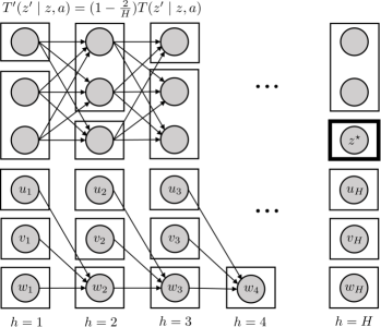
((b)) Augmented Markov Transition Model $M^{\prime}$ and aggregation scheme $\Phi^{\prime}$.

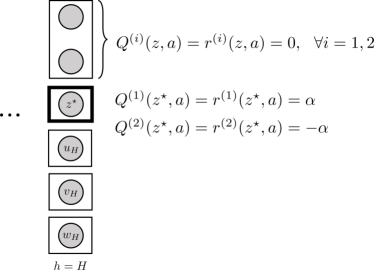
((c)) Determine the reward and value functions in the layer $H$.

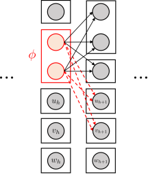
((d)) Determine the value functions inductively assuming $Q^{\scriptscriptstyle(i)}$ are already determined on all layers $h^{\prime}\geq h+1$.

Figure 4: Lower bound construction used in the proof sketch of Theorem 3.1. States are represented with circles and the corresponding state aggregations are represented with rectangles. We use the bold rectangle to denote the set of aggregations ${\mathcal{I}}$ that attains the maximum in the definition of $\bar{\mathsf{C}}_{\varepsilon}(M,\Phi,\mu)$ (see Definition 3.1). For simplicity, in the above figure $\mathcal{I}$ only contains a single aggregation that contains a single latent state ${z}^{\star}$, while in general $\mathcal{I}$ may include multiple aggregations each with multiple latent states.

1. Modified Markov Transition Model (MTM) $M^{\prime}$ (Section C.3): We construct an MTM $M^{\prime}$ with state space $\mathcal{Z}^{\prime}$ that comprises of the state space $\mathcal{Z}$ (corresponding to $M$) along with three additional states ${u}_{h},{v}_{h},{w}_{h}$ on each layer $h\in[H]$ (see Figure 4(b)). The transition dynamics $T^{\prime}$ in the $M^{\prime}$ is defined such that

   1. Each of ${u}_{h}$, ${v}_{h}$, and ${w}_{h}$ deterministically transitions to ${w}_{h+1}$ under any action.

   2. For any ${z}_{1},{z}_{2}\in\mathcal{Z}$ and $a\in\mathcal{A}$, $T^{\prime}({z}_{2}\mid{z}_{1},a)=\left(1-\nicefrac{{2}}{{H}}\right)T({z}_{2}\mid{z}_{1},a).$ In particular, the probability of each transition from $\mathcal{Z}_{h}$ to $\mathcal{Z}_{h+1}$ is decreased by a factor of $(1-\nicefrac{{2}}{{H}})$.

   3. The remaining $\nicefrac{{2}}{{H}}$ probability mass in $T^{\prime}$ is assigned to transitions from $\mathcal{Z}_{h}$ to $u_{h+1}$ and $v_{h+1}$. These transitions are different for $M^{\scriptscriptstyle(1)}$ and $M^{\scriptscriptstyle(2)}$, and will be specified later.

   Finally, we also define a new a modified aggregation scheme $\Phi^{\prime}$ that comprises of $\Phi$ along with $3H$ more singleton aggregations, each consisting of ${u}_{h},{v}_{h},{w}_{h}$ for $h\in[H]$.

2. Reward functions (Section C.2 and Section C.3): We create reward functions $r^{\scriptscriptstyle(1)}$ and $r^{\scriptscriptstyle(2)}$, for MDPs $M^{\scriptscriptstyle(1)}$ and $M^{\scriptscriptstyle(2)}$ respectively, such that non-zero rewards are only given to states in aggregation $\mathcal{I}$ and to $({u}_{h},{v}_{h},{w}_{h})_{h\in[H]}$ (see Figure 4(c)). In particular, we set

   1. $r^{\scriptscriptstyle(1)}({z},{\pi_{\mathrm{e}}}({z}))=\alpha$ and $r^{\scriptscriptstyle(2)}({z},{\pi_{\mathrm{e}}}({z}))=-\alpha$ for any state ${z}\in{\mathcal{I}}$, for some properly chosen constant $\alpha$.

   2. $r^{\scriptscriptstyle(i)}({u}_{h},a)=1$, $r^{\scriptscriptstyle(i)}({v}_{h},a)=-1$ and $r^{\scriptscriptstyle(i)}({w}_{h},a)=0$ for any $h\in[H]$ and $a\in\mathcal{A}$.

   3. $r^{\scriptscriptstyle(i)}({z},a)=0$ for all other ${z}\in\mathcal{Z}$ and $a\in\mathcal{A}$.

3. Value functions and missing transitions (Section C.2 and Section C.3): We now proceed to the construction of state-action value functions $Q^{\scriptscriptstyle(1)}$ and $Q^{\scriptscriptstyle(2)}$ for the evaluation policy ${\pi_{\mathrm{e}}}$, and the transition probabilities $T^{\scriptscriptstyle(1)}$ and $T^{\scriptscriptstyle(2)}$, for $M^{\scriptscriptstyle(1)}$ and $M^{\scriptscriptstyle(2)}$ respectively. These quantities are constructed so as to ensure that:

   1. All states that belong to the same aggregation have the same value in both $M^{\scriptscriptstyle(1)}$ and $M^{\scriptscriptstyle(2)}$, and are thus indistinguishable via the value functions, i.e. for any aggregation $\phi\in\Phi^{\prime}$, states ${z}_{1},{z}_{2}\in\phi$, and $a\in\mathcal{A}$,

      $$Q^{\scriptscriptstyle(1)}({z}_{1},{a})=Q^{\scriptscriptstyle(1)}({z}_{2},{a})\quad\text{and}\quad Q^{\scriptscriptstyle(2)}({z}_{1},{a})=Q^{\scriptscriptstyle(2)}({z}_{2},{a}).$$ (8)

   2. From any aggregation, the probability of transitioning to states ${u}_{h}$ (or to states ${v}_{h}$) is same between $M^{\scriptscriptstyle(1)}$ and $M^{\scriptscriptstyle(2)}$, i.e. for any $\phi\in\Phi$ and $h\in[H]$,

      $$\forall{a}\in{\mathcal{A}},\quad\sum_{{z}\in\phi}\mu_{h}({z},{a})T^{\scriptscriptstyle(1)}({u}_{h+1}\mid{z},{a})=\sum_{{z}\in\phi}\mu_{h}({z},{a})T^{\scriptscriptstyle(2)}({u}_{h+1}\mid{z},{a}),$$

      $$\forall{a}\in{\mathcal{A}},\quad\sum_{{z}\in\phi}\mu_{h}({z},{a})T^{\scriptscriptstyle(1)}({v}_{h+1}\mid{z},{a})=\sum_{{z}\in\phi}\mu_{h}({z},{a})T^{\scriptscriptstyle(2)}({v}_{h+1}\mid{z},{a}).$$ (9)

   3. For any ${z}_{1},{z}_{2}\in\mathcal{Z}$, we have $T^{\scriptscriptstyle(i)}({z}_{2}\mid{z}_{1},a)=T^{\prime}({z}_{2}\mid{z}_{1},a)$ for all $a\in\mathcal{A}$.

   Value functions and transitions that satisfy the above constraints are inductively constructed from time step $h=H$ to $1$. Since each of the above constraints is a linear equation, the corresponding solutions can be obtained by solving a system of linear equations. At a high level, the reason why we added ${u}_{h+1}$ and ${v}_{h+1}$ — by splitting out some transition probabilities to ${u}_{h+1}$ and ${v}_{h+1}$, and adjust their differences properly (notice that $Q^{\scriptscriptstyle(i)}({u}_{h+1},{a})=1$ and $Q^{\scriptscriptstyle(i)}({v}_{h+1},{a})=-1$), we can calibrate the state-action values in $\phi$, making them all equal.

   Jointly solving (8), (9), and using the condition $T^{\scriptscriptstyle(i)}({u}_{h+1}\mid{z},{a})+T^{\scriptscriptstyle(i)}({v}_{h+1}\mid{z},{a})=\frac{2}{H}$, we can obtain the following solution:

   $$Q^{\scriptscriptstyle(i)}(\phi,{a})=\sum_{\phi^{\prime}\in\Phi_{h+1}}\bar{T}(\phi^{\prime}\mid\phi,{a})V^{\scriptscriptstyle(i)}(\phi^{\prime}),$$ (10)

   where $Q^{\scriptscriptstyle(i)}(\phi,{a})$ is the value of $Q^{\scriptscriptstyle(i)}({z},{a})$ shared by all ${z}\in\phi$, $\Phi_{h+1}$ is the set of aggregations on layer $h+1$, and $\bar{T}(\phi^{\prime}\mid\phi,{a})=\frac{\sum_{{z}^{\prime}\in\phi^{\prime}}\sum_{{z}\in\phi}\mu_{h}({z},{a})T^{\prime}({z}^{\prime}\mid{z},{a})}{\sum_{{z}\in\phi}\mu_{h}({z},{a})}$ is the aggregated transition. This is where the aggregated transition comes into the picture. With (10), the argument that the aggregated transition plays a role in the sample complexity is similar to the argument in the tabular case as outlined in Section 3. For formal proofs, see Lemma 4$(a)$-Lemma 4$(c)$

4. Construction of offline distribution $\mu^{\prime}$ (Section C.3): For any ${z}\neq{u}_{h},{v}_{h},{w}_{h}$, we set $\mu^{\prime}_{h}({z},{a})=\frac{1}{2}\mu_{h}({z},{a})$. Furthermore, for ${z}={u}_{h},{v}_{h},{w}_{h}$, we define $\mu^{\prime}_{h}({z},{a})=\frac{1}{6}$ This construction ensures that both $\mathsf{C}$ and $\bar{\mathsf{C}}$ remain unchanged up to constant factors in the original $M$ and in the modified $M^{\scriptscriptstyle(1)}$ and $M^{\scriptscriptstyle(2)}$. See Lemma 4$(d)$ and Corollary 1 for formal proofs.

5. Lifting to block MDPs (Section C.4): We finally lift $M^{\scriptscriptstyle(1)}$ and $M^{\scriptscriptstyle(2)}$ to block MDPs where every state ${z}$ serves as a latent state invisible to the learner. Instead of observing the latent state ${z}$, the learner only observes a rich observation from the set $\mathcal{X}$ corresponding to latent state ${z}$.

For the rest of this section, we provide a formal proof for Theorem 3.1.

C.2 Construction of Aggregated MDPs

We first construct two aggregated MDPs $\bar{M}^{\scriptscriptstyle(1)}=(\Phi,\mathcal{A},\bar{T},\bar{r}^{\scriptscriptstyle(1)},H,\bar{\rho})$ and $\bar{M}^{(2)}=(\Phi,\mathcal{A},\bar{T},\bar{r}^{\scriptscriptstyle(2)},H,\bar{\rho})$ of horizon $H$, whose state space is $\Phi$ and action space is $\mathcal{A}$. Furthermore, both of them have identical transition models and initial distributions given by:

1. State Space $\Phi$, and action space $\mathcal{A}$.

2. Transition model $\bar{T}$ is defined as $\bar{T}(\phi\mid\phi,{a})\vcentcolon={}\bar{T}(\phi\mid\phi,{a};\bar{M})$, where $\bar{T}(\phi\mid\phi,{a};\bar{M})$ is given in (3).

3. Initial distribution $\bm{\bar{\rho}}$ is defined as $\bar{\rho}(\phi)\vcentcolon={}\sum_{{z}\in\phi}\rho({z})$.

Suppose $h^{*}\in[H-1]$ and set ${\mathcal{I}}\subset\Phi_{h^{*}}$ attains the maximum in Definition 3.1. The reward function of $\bar{M}^{\scriptscriptstyle(1)}$ and $\bar{M}^{\scriptscriptstyle(2)}$ are given by:

1. Reward function $\bar{r}^{\scriptscriptstyle(1)}$ for $\bar{M}^{\scriptscriptstyle(1)}$. We set the reward to be $0$ for all states $\phi\notin{\mathcal{I}}$. Furthermore, for $\phi\in{\mathcal{I}}$, we set the reward to be $0$ for actions that would not have been chosen by ${\pi_{\mathrm{e}}}$. On the remaining $(\phi,a)$ tuples, we set a non-zero reward given by:

   $$\bar{r}^{\scriptscriptstyle(1)}(\phi,{a})=\frac{\varepsilon}{2H\sum_{\phi\in{\mathcal{I}}}d_{h^{*}}^{\bar{\pi}_{\mathrm{e}}}(\phi;\bar{M})}\cdot\mathbb{I}\{\phi\in{\mathcal{I}},{a}={\pi_{\mathrm{e}}}(\phi)\},$$

   where $h^{*}$ and ${\mathcal{I}}$ are the maximizer in Definition 3.1. The key intuition in the above choice of reward function is to ensure that only those states-action contribute to non-zero rewards for which $\phi\in{\mathcal{I}}$ and $a={\pi_{\mathrm{e}}}(\phi)$; Hence, in order to receive a non-zero return, any agent in this MDP needs to first find states in ${\mathcal{I}}$ and then play action given by ${\pi_{\mathrm{e}}}$ on them. The denominator just consists of additional normalizing factors to ensure that the value is bounded by $\nicefrac{{\varepsilon}}{{2H}}$.

2. Reward function $\bar{r}^{\scriptscriptstyle(2)}$ for $\bar{M}^{\scriptscriptstyle(2)}$. The reward function is similar to $\bar{r}^{\scriptscriptstyle(1)}$, but with the negative sign. In particular, we define

   $$\bar{r}^{\scriptscriptstyle(2)}(\phi,{a})=-\frac{\varepsilon}{2H\sum_{\phi\in{\mathcal{I}}}d_{h^{*}}^{\bar{\pi}_{\mathrm{e}}}(\phi;\bar{M})}\cdot\mathbb{I}\{\phi\in{\mathcal{I}},{a}={\pi_{\mathrm{e}}}(\phi)\}.$$

Definition C.1 (Aggregated MDP).

We define aggregated MDPs $\bar{M}^{\scriptscriptstyle(1)}=(\Phi,\mathcal{A},\bar{T},\bar{r}^{\scriptscriptstyle(1)},H,\bar{\rho})$ and $\bar{M}^{(2)}=(\Phi,\mathcal{A},\bar{T},\bar{r}^{\scriptscriptstyle(2)},H,\bar{\rho})$ as follows: transition model $\bar{T}$ is defined as $\bar{T}(\phi\mid\phi,{a})\vcentcolon={}\bar{T}(\phi\mid\phi,{a};\bar{M})$, where $\bar{T}(\phi\mid\phi,{a};\bar{M})$ is given in (3), reward functions are defined as

$$\bar{r}^{\scriptscriptstyle(1)}(\phi,{a})=\frac{\varepsilon}{2H\sum_{\phi\in{\mathcal{I}}}d_{h^{*}}^{\bar{\pi}_{\mathrm{e}}}(\phi;\bar{M})}\cdot\mathbb{I}\{\phi\in{\mathcal{I}},{a}={\pi_{\mathrm{e}}}(\phi)\},$$

and,

$$\bar{r}^{\scriptscriptstyle(2)}(\phi,{a})=-\frac{\varepsilon}{2H\sum_{\phi\in{\mathcal{I}}}d_{h^{*}}^{\bar{\pi}_{\mathrm{e}}}(\phi;\bar{M})}\cdot\mathbb{I}\{\phi\in{\mathcal{I}},{a}={\pi_{\mathrm{e}}}(\phi)\}.$$

Lemma 1.

The value functions of $\bar{M}^{\scriptscriptstyle(1)}$ and $\bar{M}^{\scriptscriptstyle(2)}$ satisfies that for any policy $\pi$ and $\phi\in\Phi$,

$$V^{\pi}(\phi;\bar{M}^{\scriptscriptstyle(1)})=-V^{\pi}(\phi;\bar{M}^{\scriptscriptstyle(@)}).$$

Proof of Lemma 1. This lemma is easy to see after noticing that the transitions of $\bar{M}^{\scriptscriptstyle(1)}$ and $\bar{M}^{\scriptscriptstyle(2)}$ are the same, while the reward functions of $\bar{M}^{\scriptscriptstyle(1)}$ and $\bar{M}^{\scriptscriptstyle(2)}$ are of opposite signs. $\blacksquare$

Lemma 2.

The value functions of $\bar{M}^{\scriptscriptstyle(1)}$ and $\bar{M}^{\scriptscriptstyle(2)}$ satisfies that

$$V^{\bar{\pi}_{\mathrm{e}}}(\bar{\rho};\bar{M}^{\scriptscriptstyle(1)})=\frac{\varepsilon}{2H},\quad\text{and }V^{\bar{\pi}_{\mathrm{e}}}(\bar{\rho};\bar{M}^{\scriptscriptstyle(2)})=-\frac{\varepsilon}{2H}.$$

Additionally, for each $\phi\in\Phi$,

$$0\leq V^{\bar{\pi}_{\mathrm{e}}}(\phi;\bar{M}^{\scriptscriptstyle(1)})\leq\frac{1}{2H},\qquad-\frac{1}{2H}\leq V^{\bar{\pi}_{\mathrm{e}}}(\phi;\bar{M}^{\scriptscriptstyle(2)})\leq 0.$$ (11)

Proof of Lemma 2. According to Lemma 1, we only need to prove results for $\bar{M}^{\scriptscriptstyle(1)}$. First of all, we can write the value functions as weighted averages of rewards with occupancy-measure-weights:

$$V^{\bar{\pi}_{\mathrm{e}}}(\bar{\rho};\bar{M}^{\scriptscriptstyle(1)}) =\sum_{\phi\in{\mathcal{I}}}r^{\scriptscriptstyle(1)}(\phi,{\pi_{\mathrm{e}}}(\phi))d_{h^{*}}^{\bar{\pi}_{\mathrm{e}}}(\phi;\bar{M})=\frac{\varepsilon}{2H}.$$ (12)

Next, We let ${\mathcal{I}}$ to be the set which attains the second maximum in (2) of the definition of $\mathsf{C}_{\varepsilon}(M,\mu)$. Then ${\mathcal{I}}\subset\Phi_{h}$ for some $h\in[H-1]$, and it also satisfies $\sum_{\phi\in{\mathcal{I}}}d_{h^{*}}^{\bar{\pi}_{\mathrm{e}}}(\phi;\bar{M})\geq\varepsilon$, which implies that

$$0\leq\bar{r}^{\scriptscriptstyle(1)}(\phi,{a})\leq\frac{\varepsilon}{2H\cdot\varepsilon}\leq\frac{1}{2H},\quad\forall\phi\in\Phi_{h},a\in\mathcal{A}\qquad\text{and }\qquad\bar{r}^{\scriptscriptstyle(1)}(\phi,{a})=0,\quad\forall\phi\not\in\Phi_{h},{a}\in\mathcal{A}.$$

Hence for any $\phi\in\Phi$, the sum of rewards along any trajectory which starts from $\phi$ is always between $0$ and $\nicefrac{{1}}{{2H}}$ in $\bar{M}^{\scriptscriptstyle(1)}$. Therefore we get $0\leq V^{\bar{\pi}_{\mathrm{e}}}(\phi;\bar{M}^{\scriptscriptstyle(1)})\leq\nicefrac{{1}}{{2H}}$ for any $\phi\in\Phi$. $\blacksquare$

C.3 Construction of Latent-State MDPs and OPE Problems

Based on $\bar{M}^{\scriptscriptstyle(1)}$ and $\bar{M}^{\scriptscriptstyle(2)}$, we next construct two MDPs $M^{\scriptscriptstyle(1)}$ and $M^{\scriptscriptstyle(2)}$ which will be used as latent-state dynamics for rich observation MDPs that we construct in the next section. For $i\in\{1,2\}$, we define

$$M^{\scriptscriptstyle(i)} =\text{MDP}(\mathcal{Z}^{\prime},\mathcal{A},T^{\scriptscriptstyle(i)},r^{\scriptscriptstyle(i)},H,\rho),$$

where

1. State space $\bm{\mathcal{Z}^{\prime}}$ is defined such that $\mathcal{Z}^{\prime}=\cup_{h=1}^{H}\mathcal{Z}^{\prime}_{h}$ where, for each $h\in[H]$, in addition to the states in $\mathcal{Z}_{h}$, the set $\mathcal{Z}_{h}^{\prime}$ contains three additional states $\{{u}_{h},{v}_{h},{w}_{h}\}$ for all $h\in[H]$. Formally, $\mathcal{Z}^{\prime}_{h}\vcentcolon={}\mathcal{Z}_{h}\cup\{{u}_{h},{v}_{h},{w}_{h}\}$.

   The roles of $u_{h},v_{h}$ and $w_{h}$ is to ensure that for every aggregated state $\phi\in\Phi$, each state $z\in\phi$ has the same value functione; How we achieve this will become clear later when we define the transition model $T^{\scriptscriptstyle(i)}$.

2. Initial distribution $\bm{\rho}$ is the same as the initial distribution in $M$ (the original MDP that was used in the construction of $\bar{M}^{\scriptscriptstyle(1)}$ and $\bar{M}^{\scriptscriptstyle(2)}$).

3. Reward function $r^{\scriptscriptstyle(i)}$ is set as

   $$r^{\scriptscriptstyle(i)}({z},{a}) =\begin{cases}\bar{r}^{\scriptscriptstyle(i)}(\zeta({z}),{a})&\text{if}\quad{z}\in\mathcal{Z}_{h},\\ 1&\text{if}\quad{z}={u}_{h},\\ -1&\text{if}\quad{z}={v}_{h},\\ 0&\text{if}\quad{z}={w}_{h}.\\ \end{cases}$$

   for all $h\in[H-1]$, where $\zeta({z})$ is defined in (7). In particular, we use the same reward in $M^{\scriptscriptstyle(i)}$ as in $\bar{M}^{\scriptscriptstyle(i)}$ for the (old) states $z\in\mathcal{Z}$, and define new rewards for (newly added) states ${u}_{h},{v}_{h}$ and ${w}_{h}$. By definition, the reward $r^{\scriptscriptstyle(i)}({z}^{\prime},a)=r^{\scriptscriptstyle(i)}({z}^{\prime\prime},{a})$ whenever ${z}^{\prime}$ and ${z}^{\prime\prime}$ belong the same aggregated state $\phi$, for all ${a}\in\mathcal{A}$.

4. Transition model $\bm{T^{\scriptscriptstyle(i)}}$. The transitions are defined such that $T^{\scriptscriptstyle(i)}({z}^{\prime}\mid{z},{a})$ is proportional to $T({z}^{\prime}\mid{z},{a})$ for tuples $({z},{a},{z}^{\prime})\in\mathcal{Z}_{h}\times\mathcal{A}\times\mathcal{Z}_{h}$ that corresponds to transitions amongst (old) states that were also present in $M$, and the remaining probability mass is redirected it to new states $\{{u}_{h},{v}_{h},{w}_{h}\}_{h\in[H]}$. Formally, for ${z}\in\mathcal{Z}_{h}$ and action ${a}\in\mathcal{A}$, we set

   $$T^{\scriptscriptstyle(i)}({z}^{\prime}\mid{z},{a})=\begin{cases}\leavevmode\nobreak\ \left(1-\frac{2}{H}\right)T({z}^{\prime}\mid{z},{a})&\text{if}\quad{z}^{\prime}\in\mathcal{Z}_{h+1},\\ \leavevmode\nobreak\ [\Delta T^{\scriptscriptstyle(i)}](z)+\frac{1}{H}&\text{if}\quad{z}^{\prime}={u}_{h+1},\\ \leavevmode\nobreak\ -[\Delta T^{\scriptscriptstyle(i)}](z)+\frac{1}{H}&\text{if}\quad{z}^{\prime}={v}_{h+1},\\ \leavevmode\nobreak\ 0&\text{if}\quad{z}^{\prime}={w}_{h+1},\end{cases}$$ (13)

   where we defined

   $$[\Delta T^{\scriptscriptstyle(i)}](z)\vcentcolon={}\frac{1}{2}\left(\sum_{\phi^{\prime}\in\Phi_{h+1}}\bar{T}(\phi^{\prime}\mid\zeta({z}),{a})V^{\bar{\pi}_{\mathrm{e}}}(\phi^{\prime};\bar{M}^{\scriptscriptstyle(i)})-\left(1-\frac{2}{H}\right)\sum_{{z}^{\prime}\in\mathcal{Z}_{h+1}}T({z}^{\prime}\mid{z},{a})V^{\bar{\pi}_{\mathrm{e}}}(\zeta({z}^{\prime});\bar{M}^{\scriptscriptstyle(i)})\right).$$ (14)

   Furthermore, for any ${z}\in\{{u}_{h},{v}_{w},{w}_{h}\}$ and ${a}\in\mathcal{A}$, $T^{\scriptscriptstyle(i)}$ transits to $w_{h+1}$ with probability $1$, i.e.

   $$T^{\scriptscriptstyle(i)}({z}^{\prime}\mid{z},{a})=\begin{cases}\leavevmode\nobreak\ 1&\text{if}\quad{z}^{\prime}={w}_{h+1}\\ \leavevmode\nobreak\ 0&\text{otherwise}\end{cases}$$ (15)

   Intuitively, the above transitions imply that states $\{{w}_{h}\}_{h\in[H-1]}$ act as terminal states.

We further define distribution $\mu_{h}^{\prime}$ over $\mathcal{Z}_{h}^{\prime}$ of layer $h\in[H-1]$ as follows:

$$\mu^{\prime}_{h}({z})=\begin{cases}\frac{\mu_{h}({z})}{2}&\text{if}\quad{z}\in\mathcal{Z}_{h},\\ \frac{1}{6}&\text{if}\quad{z}\in\{{u}_{h},{v}_{h},{w}_{h}\}.\end{cases}$$ (16)

Additionally, to be formal, we define ${\pi_{b}}({z})={\pi_{\mathrm{e}}}({z})\equiv a_{0}$ (an arbitrary fixed state in $\mathcal{A}$) for any ${z}\in\{{u}_{h},{v}_{h},{w}_{h}\}$, and the OPE problems $\mathfrak{g}^{\scriptscriptstyle(1)}$ and $\mathfrak{g}^{\scriptscriptstyle(2)}$ as

$$\mathfrak{g}^{\scriptscriptstyle(1)}=\textsc{OPE}(M^{\scriptscriptstyle(1)},{\pi_{\mathrm{e}}},\mu^{\prime},\mathcal{F}),\quad\mathfrak{g}^{\scriptscriptstyle(2)}=\textsc{OPE}(M^{\scriptscriptstyle(2)},{\pi_{\mathrm{e}}},\mu^{\prime},\mathcal{F}),$$ (17)

where $\mathcal{F}\vcentcolon={}\{Q^{\scriptscriptstyle(1)},Q^{\scriptscriptstyle(2)}\}$ with $Q^{\scriptscriptstyle(1)}$ and $Q^{\scriptscriptstyle(2)}$ are state-action value functions of $M^{\scriptscriptstyle(1)}$ and $M^{\scriptscriptstyle(2)}$ under policy ${\pi_{\mathrm{e}}}$. Before we proceed, we note the following technical lemma.

Lemma 3.

For $i\in\{1,2\}$, $T^{\scriptscriptstyle(i)}$ constructed via (13) and (15) above is a valid transition model.

Proof of Lemma 3. We first show that $T^{\scriptscriptstyle(i)}({z}^{\prime}\mid{z},{a})>0$ for all ${a}\in\mathcal{A}$ and ${z},{z}^{\prime}\in\mathcal{Z}^{\prime}_{h+1}$. This is trivial for ${z}^{\prime}\in\mathcal{Z}_{h}$ or when ${z}^{\prime}={w}_{h+1}$. We next show that the same holds when ${z}^{\prime}\in\{{u}_{h+1},{v}_{h+1}\}$.

Note that due to Lemma 2, we have that $\lvert V^{\bar{\pi}_{\mathrm{e}}}(\phi;\bar{M}^{\scriptscriptstyle(i)})\rvert\leq\frac{1}{2H}$ for all $\phi\in\Phi$. Plugging this in (14), and using Triangle inequality, we get that

$$\left\lvert[\Delta T^{\scriptscriptstyle(i)}](z)\right\rvert\leq\sup_{\phi\in\Phi}\left\lvert V^{\bar{\pi}_{\mathrm{e}}}(\phi;\bar{M}^{\scriptscriptstyle(i)})\right\rvert\leq\frac{1}{2H}.$$

Using this in (13), we immediately get that $T^{\scriptscriptstyle(i)}({z}^{\prime}\mid{z},{a})>0$ for any $\varepsilon\leq 1$. Furthermore, it is easy to check that for any ${z}\in\mathcal{Z}^{\prime}_{h}$ and $a\in\mathcal{A}$, $\sum_{{z}^{\prime}\in\mathcal{Z}^{\prime}_{h+1}}T^{\scriptscriptstyle(i)}({z}^{\prime}\mid{z},{a})=1.$ Thus, $T^{\scriptscriptstyle(i)}$ is a valid transition model. $\blacksquare$

We note the following technical lemma, which will be used in the rest of the analysis.

Lemma 4.

We have the following properties of value functions, state-action value functions and occupancy measures of $M^{\scriptscriptstyle(1)}$ and $M^{\scriptscriptstyle(2)}$:

1. For $i\in\{1,2\}$, and for any $\phi\in\Phi$, ${z}\in\phi$, and $a\in\mathcal{A}$,

   $$Q^{\pi_{\mathrm{e}}}({z},{a};M^{\scriptscriptstyle(i)})=Q^{\bar{\pi}_{\mathrm{e}}}(\zeta({z}),{a};\bar{M}^{\scriptscriptstyle(i)}).$$

2. Corresponding to the initial distribution $\rho$, the expected values satisfy

   $$V^{\pi_{\mathrm{e}}}(\rho;M^{\scriptscriptstyle(1)})-V^{\pi_{\mathrm{e}}}(\rho;M^{\scriptscriptstyle(2)})=\frac{\varepsilon}{H}.$$

3. For any $h\in[H-1]$, latent state $\phi\in\Phi_{h}$, action ${a}\in\mathcal{A}$ and latent state ${z}^{\prime}\in\mathcal{Z}^{\prime}$,

   $$\sum_{{z}\in\phi}\mu({z}\mid{z}\in\phi,{a})T^{\scriptscriptstyle(1)}({z}^{\prime}\mid{z},{a})=\sum_{{z}\in\phi}\mu({z}\mid{z}\in\phi,{a})T^{\scriptscriptstyle(2)}({z}^{\prime}\mid{z},{a}).$$

4. For each $i\in\{1,2\}$, for any $h\in[H-1]$ and ${z}\in\mathcal{Z}_{h}$, and policy $\pi$,

   $$\frac{1}{16}d_{h}^{\pi}({z};M)\leq d_{h}^{\pi}({z};M^{\scriptscriptstyle(i)})\leq d_{h}^{\pi}({z};M).$$

Proof of Lemma 4. Observe that, by construction, we have for $i\in\{1,2\}$,

$$Q^{\scriptscriptstyle(i)}({u}_{h},{a})=1,\qquad Q^{\scriptscriptstyle(i)}({v}_{h},{a})=-1,\text{and}\qquad Q^{\scriptscriptstyle(i)}({w}_{h},{a})=0,$$

for any $h$ and ${a}\in\mathcal{A}$.

Proof of $(a)$:

The proof follows via downward induction from $h=H$ to $h=1$. First note that for any ${z}\in\mathcal{Z}_{H}$ and $a\in\mathcal{A}$, we have $Q^{\pi_{\mathrm{e}}}({z},{a};M^{\scriptscriptstyle(i)})=0=Q^{\bar{\pi}_{\mathrm{e}}}(\zeta({z}),{a};\bar{M}^{\scriptscriptstyle(i)})$; Thus the base case is satisfied. For the induction hypotesis, assume that the desired claim holds for $h+1$. Thus, for layer $h$, using Bellman equation for the policy ${\pi_{\mathrm{e}}}$, we have that

$$Q^{\pi}({z},{a};M^{\scriptscriptstyle(i)})$$

$$=r^{\scriptscriptstyle(i)}({z},{a})+T^{\scriptscriptstyle(i)}({u}_{h+1}\mid{z},{a})-T^{\scriptscriptstyle(i)}({v}_{h+1}\mid{z},{a})+\sum_{{z}^{\prime}\in\mathcal{Z}_{h+1}}T^{\scriptscriptstyle(i)}({z}^{\prime}\mid{z},{a})Q^{\pi_{\mathrm{e}}}({z}^{\prime},{\pi_{\mathrm{e}}}({z}^{\prime});M^{\scriptscriptstyle(i)})$$

$$=\bar{r}^{\scriptscriptstyle(i)}(\zeta({z}),{a})+T^{\scriptscriptstyle(i)}({u}_{h+1}\mid{z},{a})-T^{\scriptscriptstyle(i)}({v}_{h+1}\mid{z},{a})+\sum_{{z}^{\prime}\in\mathcal{Z}_{h+1}}T^{\scriptscriptstyle(i)}({z}^{\prime}\mid{z},{a})V^{\bar{\pi}_{\mathrm{e}}}(\zeta({z}^{\prime});\bar{M}^{\scriptscriptstyle(i)})$$

$$=\bar{r}^{\scriptscriptstyle(i)}(\zeta({z}),{a})+\sum_{\phi^{\prime}\in\Phi_{h+1}}\bar{T}(\phi^{\prime}\mid\zeta({z}),{a})V^{\bar{\pi}_{\mathrm{e}}}(\phi^{\prime};\bar{M}^{\scriptscriptstyle(i)})$$

$$=Q^{\bar{\pi}_{\mathrm{e}}}(\zeta({z}),{a};\bar{M}^{\scriptscriptstyle(i)}),$$

where in the last line, we used Bellman equation for policy ${\pi_{\mathrm{e}}}$ under the MDP $\bar{M}^{\scriptscriptstyle(1)}$. The above completes the induction step, thus showing that the claim holds for all $h\in[H]$.

Proof of $(b)$:

Using part-$(a)$ above, we note that

$$V^{\pi_{\mathrm{e}}}({z};M^{\scriptscriptstyle(1)})=Q^{\pi_{\mathrm{e}}}({z},{\pi_{\mathrm{e}}}({z});M^{\scriptscriptstyle(1)})=Q^{\bar{\pi}_{\mathrm{e}}}(\zeta({z}),{\bar{\pi}_{\mathrm{e}}}(\zeta({z}));\bar{M}^{\scriptscriptstyle(1)})=V^{\bar{\pi}_{\mathrm{e}}}(\zeta({z});\bar{M}^{\scriptscriptstyle(1)}).$$

Similarly, we also get that $V^{\pi_{\mathrm{e}}}({z};M^{\scriptscriptstyle(2)})=V^{\bar{\pi}_{\mathrm{e}}}(\zeta({z});\bar{M}^{\scriptscriptstyle(2)})$. The desired bound follows by noting that (12) implies

$$V^{\bar{\pi}_{\mathrm{e}}}(\bar{\rho};\bar{M}^{\scriptscriptstyle(1)})-V^{\bar{\pi}_{\mathrm{e}}}(\bar{\rho};\bar{M}^{\scriptscriptstyle(2)})=\frac{\varepsilon}{H},$$

which implies

$$V^{\pi_{\mathrm{e}}}(\rho;M^{\scriptscriptstyle(1)})-V^{\pi_{\mathrm{e}}}(\rho;M^{\scriptscriptstyle(2)})=\frac{\varepsilon}{H}.$$

Proof of $(c)$:

First note that whenever ${z}^{\prime}\not\in\{{u}_{h},{v}_{h}\}_{h=1}^{H}$, we always have $T^{\scriptscriptstyle(1)}({z}^{\prime}\mid{z},{a})=T^{\scriptscriptstyle(2)}({z}^{\prime}\mid{z},{a})$ according to the definition of $T^{\scriptscriptstyle(1)}$ and $T^{\scriptscriptstyle(2)}$. We next show that the same holds for ${z}^{\prime}={u}_{h}$. We only need to verify $\sum_{{z}\in\phi}\mu({z},{a})(T^{\scriptscriptstyle(1)}({u}_{h}\mid{z},{a})-T^{\scriptscriptstyle(2)}({u}_{h}\mid{z},{a}))=0$.

$$\quad\sum_{{z}\in\phi}\mu({z},{a})(T^{\scriptscriptstyle(1)}({u}_{h}\mid{z},{a})-T^{\scriptscriptstyle(2)}({u}_{h}\mid{z},{a}))$$

$$=\sum_{{z}\in\phi}\mu({z},{a})\left(\sum_{\phi^{\prime}\in\Phi_{h+1}}\bar{T}(\phi^{\prime}\mid\zeta({z}),{a})\bar{V}^{\scriptscriptstyle(1)}(\phi^{\prime})-\sum_{{z}^{\prime}\in\mathcal{Z}_{h+1}}T^{\scriptscriptstyle(1)}({z}^{\prime}\mid{z},{a})\bar{V}^{\scriptscriptstyle(1)}(\zeta({z}^{\prime}))\right)$$

$$=\sum_{{z}\in\phi}\mu({z},{a})\sum_{\phi^{\prime}\in\Phi_{h+1}}\bar{T}(\phi^{\prime}\mid\phi,{a})\bar{V}^{\scriptscriptstyle(1)}(\phi^{\prime})-\sum_{\phi^{\prime}\in\Phi_{h+1}}\sum_{{z}^{\prime}\in\phi^{\prime}}\bar{V}^{\scriptscriptstyle(1)}(\zeta({z}^{\prime}))\sum_{{z}\in\phi}\mu({z},{a})T^{\scriptscriptstyle(1)}({z}^{\prime}\mid{z},{a})$$

$$=\sum_{{z}\in\phi}\mu({z},{a})\sum_{\phi^{\prime}\in\Phi_{h+1}}\bar{T}(\phi^{\prime}\mid\phi,{a})\bar{V}^{\scriptscriptstyle(1)}(\phi^{\prime})-\sum_{\phi^{\prime}\in\Phi_{h+1}}\bar{V}^{\scriptscriptstyle(1)}(\phi^{\prime})\sum_{{z}^{\prime}\in\phi^{\prime}}\sum_{{z}\in\phi}\mu({z},{a})T^{\scriptscriptstyle(1)}({z}^{\prime}\mid{z},{a})$$

$$=\sum_{{z}\in\phi}\mu({z},{a})\sum_{\phi^{\prime}\in\Phi_{h+1}}\bar{T}(\phi^{\prime}\mid\phi,{a})\bar{V}^{\scriptscriptstyle(1)}(\phi^{\prime})-\sum_{\phi^{\prime}\in\Phi_{h+1}}\bar{V}^{\scriptscriptstyle(1)}(\phi^{\prime})\sum_{{z}\in\phi}\mu({z},{a})\bar{T}(\phi^{\prime}\mid\phi,{a})$$

$$=0,$$

where the first equation uses the definition of $T^{\scriptscriptstyle(1)}$ and $T^{\scriptscriptstyle(2)}$ in (13) and Lemma 1, and the last equation follows from the definition of $\bar{T}$ in (3). Hence $(c)$ is verified for ${z}^{\prime}={u}_{h}$. The proof for ${z}^{\prime}={v}_{h}$ follows similarly.

Proof of $(d)$:

We only prove the result for $M^{\scriptscriptstyle(1)}$; the proof for $M^{\scriptscriptstyle(2)}$ follows similarly. In fact, we show a slightly stronger result that for all $h\in[H]$ and ${z}\in\mathcal{Z}_{h}$,

$$\left(\frac{H-2}{H}\right)^{h-1}d_{h}^{\pi}({z};M)\leq d_{h}^{\pi}({z};M^{\scriptscriptstyle(1)})\leq d_{h}^{\pi}({z};M).$$ (18)

The proof follows via induction over $h$. For the base case, note that for $h=1$, by definition, we have $d_{1}^{\pi}({z};M)=\rho({z})=d_{1}^{\pi}({z};M^{\scriptscriptstyle(1)})$ for any ${z}\in\mathcal{Z}_{1}$, which implies (18).

For the induction step, suppose (18) holds for a certain $h\leq H-1$. For the upper bound, note that any ${z}\in\mathcal{Z}_{h+1}$ satisfies

$$d_{h+1}^{\pi}({z};M^{\scriptscriptstyle(1)})=\sum_{{z}^{\prime}\in\mathcal{Z}_{h}}d_{h}^{\pi}({z}^{\prime};M^{\scriptscriptstyle(1)})T^{\scriptscriptstyle(1)}({z}\mid{z}^{\prime},\pi({z}^{\prime})),$$

which combined with the upper bound in (18) implies

$$d_{h+1}^{\pi}({z};M^{\scriptscriptstyle(1)}) \leq\sum_{{z}^{\prime}\in\mathcal{Z}_{h}}d_{h}^{\pi}({z}^{\prime};M)T({z}\mid{z}^{\prime},\pi({z}^{\prime}))=d_{h+1}^{\pi}({z};M).$$

For the lower bound, recall from the definition of $T^{\scriptscriptstyle(1)}$, which implies that

$$T^{\scriptscriptstyle(1)}({z}\mid{z}^{\prime},\pi({z}^{\prime}))=\frac{H-2}{H}T({z}\mid{z}^{\prime},\pi({z}^{\prime})).$$

Using the above with the lower bound in (18), we get that

$$d_{h+1}^{\pi}({z};M^{\scriptscriptstyle(1)}) =\sum_{{z}^{\prime}\in\mathcal{Z}_{h}^{\prime}}d_{h}^{\pi}({z}^{\prime};M^{\scriptscriptstyle(1)})T^{\scriptscriptstyle(1)}({z}\mid{z}^{\prime},\pi({z}^{\prime}))$$

$$\geq\left(\frac{H-2}{H}\right)^{h-1}\sum_{{z}^{\prime}\in\mathcal{Z}_{h}}d_{h}^{\pi}({z}^{\prime};M)\cdot\frac{H-2}{H}T({z}\mid{z}^{\prime},\pi({z}^{\prime}))=\left(\frac{H-2}{H}\right)^{h}d_{h}^{\pi}({z};M).$$

The two bounds above imply the (18) also holds for $h+1$. This completes the induction step. $\blacksquare$

This lemma has two direct corollaries:

Corollary 1.

The concentratbility coefficients $\mathsf{C}(M^{\scriptscriptstyle(1)},\mu^{\prime})$ and $\mathsf{C}(M^{\scriptscriptstyle(2)},\mu^{\prime})$ of $M^{\scriptscriptstyle(1)}$ and $M^{\scriptscriptstyle(2)}$, respectively, satisfy that

$$\mathsf{C}(M^{\scriptscriptstyle(1)},\mu^{\prime})\leq 6\mathsf{C}(M,\mu,{\pi_{\mathrm{e}}})\quad\text{and}\quad\mathsf{C}(M^{\scriptscriptstyle(2)},\mu^{\prime})\leq 6\mathsf{C}(M,\mu,{\pi_{\mathrm{e}}}).$$

Proof of Corollary 1. This corollary directly follows from Definition 16 and Lemma 4 $(d)$. $\blacksquare$

Corollary 2.

For any two policies $\pi$ and $\pi^{\prime}$ and any $i\in\{1,2\}$, we have

$$\sup_{h\in[H]}\sup_{{z}\in\mathcal{Z}_{h}^{\prime}}\frac{d_{h}^{\pi}({z};M^{\scriptscriptstyle(i)})}{d_{h}^{\pi^{\prime}}({z};M^{\scriptscriptstyle(i)})}\leq 48\cdot\sup_{h\in[H]}\sup_{{z}\in\mathcal{Z}_{h}}\frac{d_{h}^{\pi}({z};M)}{d_{h}^{\pi^{\prime}}({z};M)}$$

Proof of Corollary 2. First of all, for those ${z}\in\mathcal{Z}_{h}$ and $h\in[H-1]$, Lemma 4 $(d)$ indicates that

$$\frac{d_{h}^{\pi}({z};M^{\scriptscriptstyle(i)})}{d_{h}^{\pi^{\prime}}({z};M^{\scriptscriptstyle(i)})}\leq 16\cdot\frac{d_{h}^{\pi}({z};M)}{d_{h}^{\pi^{\prime}}({z};M)}\leq 48\cdot\sup_{h\in[H]}\sup_{{z}\in\mathcal{Z}_{h}}\frac{d_{h}^{\pi}({z};M)}{d_{h}^{\pi^{\prime}}({z};M)}.$$

Next, we verify cases where ${z}\in\{{u}_{h},{v}_{h},{w}_{h}\}_{h=1}^{H}$. Notice that the transition model of $M^{\scriptscriptstyle(i)}$ gives that

$$d_{h}^{\pi}({w}_{h};M^{\scriptscriptstyle(i)})=d_{h-1}^{\pi}({u}_{h};M^{\scriptscriptstyle(i)})+d_{h-1}^{\pi}({v}_{h-1};M^{\scriptscriptstyle(i)}),$$

we only need to verify that for any ${z}\in\{{u}_{h},{v}_{h}\}_{h=1}^{H}$, we have

$$\frac{d_{h}^{\pi}({z};M^{\scriptscriptstyle(i)})}{d_{h}^{\pi^{\prime}}({z};M^{\scriptscriptstyle(i)})}\leq 48\cdot\sup_{h\in[H]}\sup_{{z}\in\mathcal{Z}_{h}}\frac{d_{h}^{\pi}({z};M)}{d_{h}^{\pi^{\prime}}({z};M)}.$$

Without loss of generality, we only verify for ${z}={u}_{h}$. We write

$$d_{h}^{\pi}({u}_{h};M^{\scriptscriptstyle(i)})=\sum_{{z}\in\mathcal{Z}_{h-1}}T^{\scriptscriptstyle(i)}({u}_{h}\mid{z},\pi({z}))d_{h-1}^{\pi}({z}).$$

According to the transition model of $M^{\scriptscriptstyle(i)}$, we have for any ${z}\in\mathcal{Z}_{h-1}$ and any ${a}\in\mathcal{A}$,

$$T^{\scriptscriptstyle(i)}({u}_{h}\mid{z},{a})\in\left[\frac{1}{2H},\frac{3}{2H}\right],$$

which indicates that for any policy $\pi,\pi^{\prime}$, we have

$$\sup_{{z}\in\mathcal{Z}_{h-1}}\frac{T^{\scriptscriptstyle(i)}({u}_{h}\mid{z},\pi({z}))}{T^{\scriptscriptstyle(i)}({u}_{h}\mid{z},\pi^{\prime}({z}))}\in[1,3].$$

Therefore, we have

$$\frac{d_{h}^{\pi}({u}_{h};M^{\scriptscriptstyle(i)})}{d_{h}^{\pi^{\prime}}({u}_{h};M^{\scriptscriptstyle(i)})}\leq 3\cdot\sup_{{z}\in\mathcal{Z}_{h-1}}\frac{d_{h-1}^{\pi}({z};M^{\scriptscriptstyle(i)})}{d_{h-1}^{\pi^{\prime}}({z};M^{\scriptscriptstyle(i)})}\leq 48\cdot\sup_{h\in[H]}\sup_{{z}\in\mathcal{Z}_{h}}\frac{d_{h}^{\pi}({z};M)}{d_{h}^{\pi^{\prime}}({z};M)},$$

where the last inequality follows from Lemma 4 $(d)$. $\blacksquare$

C.4 Construction of the Class $\mathfrak{G}$ of Offline Policy Evaluation Problems

In this section, we construct the class $\mathfrak{G}$ of OPE problems that are used in Theorem 3.1. The corresponding MDPs in $\mathfrak{G}$ are block MDPs based on $M^{\scriptscriptstyle(1)}$ and $M^{\scriptscriptstyle(2)}$ (constructed in the previous section), and certain decoder functions. The organization of this section is as follows:

1. In Appendix C.4.1, we provide a general procedure to lift an OPE problem $\textsc{OPE}(M,{\pi_{\mathrm{e}}},\mu,\mathcal{F})$ over state space $\mathcal{Z}$ into a block OPE problem $(\check{M},{\check{\pi}_{\mathrm{e}}},\check{\mu},\check{\mathcal{F}})$ with rich-observations in a set $\mathcal{X}$ and latent states in $\mathcal{Z}$, given a decoder function $\psi$.

2. Then, in Appendix C.4.2, we first provide a class $\Psi$ of decoder function and use the above procedure to construct the family $\mathfrak{G}$ of offline RL problems.

C.4.1 Lifting from OPE Problems to Block OPE Problems

In this section, we will discuss how to lift a normal OPE problem $\textsc{OPE}(M,{\pi_{\mathrm{e}}},\mu,\mathcal{F})$ ($\mathcal{F}$ satisfies $Q$-realizability) into a block OPE problem $\textsc{OPE}(\check{M},{\check{\pi}_{\mathrm{e}}},\check{\mu},\check{\mathcal{F}})$ where $\check{\mathcal{F}}$ satisfies $(Q,W)$-realizability.

Let $\mathcal{Z}=\bigcup_{h\in[H-1]}\mathcal{Z}_{h}$ be the state space of MDP $M$, and we fix $\mathcal{X}=\{\mathcal{X}({z})\}_{{z}\in\mathcal{Z}}$ to be a family of disjoint sets that denote rich-observations corresponding to latent states ${z}\in\mathcal{Z}$. Furthermore, let $\mathcal{X}_{h}=\{\mathcal{X}({z})\}_{{z}\in\mathcal{Z}_{h}}$. Then, for $M=\textsc{MDP}(\mathcal{Z},\mathcal{A},T,r,H,\rho)$, we can define a block MDP

$$\check{M}=\text{MDP}(\mathcal{X},\mathcal{A},\check{T},\check{R},H,\check{\rho})$$

with latent state $\mathcal{Z}$ and rich observations in $\mathcal{X}$, where

• State space: $\mathcal{X}$ consists of rich-observations corresponding to latent states. We assume that the state space $\mathcal{X}=\bigcup_{h\in[H-1]}\mathcal{X}_{h}$ is layered.

• Transition Model depends only on the latent transition model $T$. In particular, for any $h\in[H-1]$, ${x}\in\mathcal{X}({z})$ corresponding to ${z}\in\mathcal{Z}_{h}$, and ${x}^{\prime}\in\mathcal{X}({z}^{\prime})$ corresponding to ${z}^{\prime}\in\mathcal{Z}_{h+1}$, we have

  $$\check{T}({x}^{\prime}\mid{x},{a})\vcentcolon={}\frac{1}{|\mathcal{X}({z}^{\prime})|}\cdot T({z}^{\prime}\mid{z},{a}).$$

• Rewards: For any ${z}\in\mathcal{Z}$ and ${x}\in\mathcal{X}$, and ${a}\in\mathcal{A}$, $\check{R}({x},{a})$ is a $\{-1,1\}$-valued random variable with expected value $r({z},{a})$.

• Initial distribution: $\check{\rho}\in\Delta(\mathcal{X}_{1})$ is defined such that for any $x\in\mathcal{X}_{1}$,

  $$\check{\rho}({x})\vcentcolon={}\frac{1}{|\mathcal{X}({z})|}\cdot\rho({z})$$ (19)

  where ${z}$ is such that ${x}\in\mathcal{X}({z})$.

In particular, corresponding to a latent state ${z}$, the observations are sampled from $\text{Uniform}(\mathcal{X}(z))$. In order to construct respective offline RL problems on the MDP $\check{M}$, we also lift the offline data distribution $\mu$ to $\check{\mu}$, and offline policy ${\pi_{\mathrm{e}}}$ to ${\check{\pi}_{\mathrm{e}}}$ as follows:

• Offline distribution For any $h\in[H-1]$, we define $\check{\mu}_{h}\in\Delta(\mathcal{X}_{h}\times\mathcal{A})$ such that for any $x\in\mathcal{X}_{h}$ and $a\in\mathcal{A}$,

  $$\check{\mu}_{h}({x},{a})\vcentcolon={}\frac{1}{|\mathcal{X}({z})|}\cdot\mu_{h}({z},{a}),$$

  where ${z}\in\mathcal{Z}_{h}$ is such that ${x}\in\mathcal{X}({z})$.

• Evaluation policy ${\check{\pi}_{\mathrm{e}}}:\mathcal{X}\mapsto\mathcal{A}$ is defined such that for any ${x}\in\mathcal{X}$, ${\check{\pi}_{\mathrm{e}}}({x})\vcentcolon={}{\pi_{\mathrm{e}}}({z})$ where ${z}$ is such that ${x}\in\mathcal{X}({z})$.

• Function class $\check{\mathcal{F}}$ consists of tuples $(\check{f},\check{W})$, where each $f\in\mathcal{F}$ generates a tuple $(\check{f},\check{W})$ with $\check{f}:\mathcal{X}\times\mathcal{A}\to\mathbb{R}$ defined as $\check{f}({x},{a})=f({z},{a})$ for any ${x}\in\mathcal{X}({z})$ and $\check{W}:[H-1]\to\mathbb{R}$ is defined as $\check{W}[H-1]=\sum_{{x}\in\mathcal{X}_{h}}\check{\mu}_{h}({x},{\check{\pi}_{\mathrm{e}}}({x}))\check{f}({x},{\check{\pi}_{\mathrm{e}}}({a}))$.

The following lemma indicates that $\check{f}$ is the state-action value function of block MDP $\check{M}$ as long as $f$ is the state-action value function of MDP $M$.

Lemma 5.

For any $h\in[H]$, ${z}\in\mathcal{Z}_{h}$, $x\in\mathcal{X}({z})$ and $a\in\mathcal{A}$, we have

$$Q_{h}^{{\check{\pi}_{\mathrm{e}}}}({x},{a};\check{M})=Q_{h}^{\pi_{\mathrm{e}}}({z},{a};M).$$

Proof of Lemma 5. We prove this equation by induction from $h=H$ to $h=1$. When $h=H$, we have $Q_{H}^{{\check{\pi}_{\mathrm{e}}}}({x},{a};\check{M})=Q_{H}^{\pi_{\mathrm{e}}}({z},{a};M)$ for any ${z}\in\mathcal{Z}_{H}$, ${z}\in\mathcal{X}({z})$ and ${a}\in\mathcal{A}$. Next, suppose $Q_{h+1}^{{\check{\pi}_{\mathrm{e}}}}({x},{a};\check{M})=Q_{h+1}^{\pi_{\mathrm{e}}}({z},{a};M)$ holds for ${z}\in\mathcal{Z}_{h+1}$ and ${x}\in\mathcal{X}({z})$. According to the Bellman equation and definitions of $\check{T},\check{R}$, for any ${z}\in\mathcal{Z}_{h}$ and ${x}\in\mathcal{X}({z})$, we have

$$Q_{h}^{\check{\pi}_{\mathrm{e}}}({x},{a};\check{M}) =\mathbb{E}[\check{R}({x},{a})]+\sum_{{x}^{\prime}\in\mathcal{X}_{h+1}}\check{T}({x}^{\prime}\mid{x},{a})Q_{h+1}^{\check{\pi}_{\mathrm{e}}}({x}^{\prime},{\check{\pi}_{\mathrm{e}}}({x}^{\prime});\check{M})$$

$$=r({z},{a})+\sum_{{z}^{\prime}\in\mathcal{Z}_{h+1}}Q_{h+1}^{\pi_{\mathrm{e}}}({z}^{\prime},{\pi_{\mathrm{e}}}({z}^{\prime}))\sum_{{x}^{\prime}\in\mathcal{X}({z}^{\prime})}\check{T}({x}^{\prime}\mid{x},{a})$$

$$=r({z},{a})+\sum_{{z}^{\prime}\in\mathcal{Z}_{h+1}}Q_{h+1}^{\pi_{\mathrm{e}}}({z}^{\prime},{\pi_{\mathrm{e}}}({z}^{\prime});M)\sum_{{z}^{\prime}\in\phi^{\prime}}T({z}^{\prime}\mid{z},{a})$$

$$=Q_{h}^{\pi_{\mathrm{e}}}({z},{a};M),$$

where we use the induction hypothesis and the fact that ${\check{\pi}_{\mathrm{e}}}({x}^{\prime})={\pi_{\mathrm{e}}}({z})$ for ${x}^{\prime}\in\mathcal{X}({z}^{\prime})$ in the second equation.

$\blacksquare$

Lemma 6.

For any $h\in[H-1]$,

$$\sum_{{x}\in\mathcal{X}_{h}}\check{\mu}_{h}({x},{\check{\pi}_{\mathrm{e}}}({x}))Q_{h}^{\check{\pi}_{\mathrm{e}}}({x},{\check{\pi}_{\mathrm{e}}}({x});\check{M})=\sum_{{z}\in\mathcal{Z}_{h}}\mu_{h}({z},{\pi_{\mathrm{e}}}({z}))Q_{h}^{\pi_{\mathrm{e}}}({z},{\pi_{\mathrm{e}}}({x});M).$$

Proof of Lemma 6. We first notice that ${x}\in\mathcal{X}({z})$, we have ${\check{\pi}_{\mathrm{e}}}({x})={\pi_{\mathrm{e}}}({z})$. Hence according to Lemma 5 we only need to verify that, for any ${z}\in\mathcal{Z}$,

$$\sum_{{x}\in\mathcal{X}({z})}\check{\mu}_{h}({x},{\check{\pi}_{\mathrm{e}}}({x}))=\mu_{h}({z},{\pi_{\mathrm{e}}}({z})),$$

which is given by definition $\check{\mu}_{h}({x},{a})\vcentcolon={}\frac{\mu_{h}({z},{a})}{|\mathcal{X}({z})|}$. $\blacksquare$

Lemma 7.

For any policy $\pi$ over MDP $M$, let policy $\check{\pi}$ over $\check{M}$ to be $\check{\pi}({x})=\pi({z})$ for any ${x}\in\mathcal{X}({z})$. Then we have for any $h\in[H]$, ${z}\in\mathcal{Z}_{h}$ and ${x}\in\mathcal{X}({z})$,

$$d_{h}^{\check{\pi}}({x};\check{M})=\frac{d_{h}^{\pi}({z};M)}{|\mathcal{X}({z})|}.$$ (20)

Proof of Lemma 7. We will prove via induction on the layer of ${x}$. For ${x}\in\mathcal{X}_{1}$, (20) holds acording to the definition of initial distribution $\check{\rho}$. The induction from layer $h$ to layer $h+1$ can be achieved by

$$d_{h+1}^{\check{\pi}}({x};\check{M})=\sum_{{x}^{\prime}\in\mathcal{X}_{h}}d_{h}^{\check{\pi}}({x}^{\prime};\check{M})\check{T}({x}\mid{x}^{\prime},\check{\pi}({x}^{\prime}))=\sum_{{z}^{\prime}\in\mathcal{Z}_{h}}d_{h}^{\pi}({z}^{\prime};M)\frac{T({z}\mid{z}^{\prime},\pi({z}^{\prime}))}{|\mathcal{X}({z})|}=\frac{d_{h}^{\pi}({z};M)}{|\mathcal{X}({z})|}$$

for any ${x}\in\mathcal{X}({z})$ and ${z}\in\mathcal{Z}_{h+1}$. $\blacksquare$

The above lemma has the following two corollaries:

Corollary 3.

The concentrability coefficient $\mathsf{C}(\check{M},\mu,{\check{\pi}_{\mathrm{e}}})=\mathsf{C}(M,\mu,{\pi_{\mathrm{e}}})$.

Proof of Corollary 3. According to Lemma 7, we have for any $h\in[H-1]$, ${z}\in\mathcal{Z}_{h}$ and ${x}\in\mathcal{X}({z})$,

$$\frac{d_{h}^{{\check{\pi}_{\mathrm{e}}}}({x};\check{M})}{\check{\mu}({x})}=\frac{\nicefrac{{d_{h}^{\pi_{\mathrm{e}}}({z};M)}}{{|\mathcal{X}({z})|}}}{\nicefrac{{\mu({z})}}{{|\mathcal{X}({z})|}}}=\frac{d_{h}^{\pi_{\mathrm{e}}}({z};M)}{\mu({z})}.$$

Taking the supremum over all $h\in[H-1]$, ${z}\in\mathcal{Z}_{h}$ and ${x}\in\mathcal{X}({z})$, we get

$$\mathsf{C}(\check{M},\mu,{\check{\pi}_{\mathrm{e}}})=\sup_{h\in[H-1]}\sup_{{x}\in\mathcal{X}_{h}}\frac{d_{h}^{{\check{\pi}_{\mathrm{e}}}}({x};\check{M})}{\check{\mu}({x})}=\sup_{h\in[H-1]}\sup_{{z}\in\mathcal{Z}_{h}}\frac{d_{h}^{\pi_{\mathrm{e}}}({z};M)}{\mu({z})}=\mathsf{C}(M,\mu,{\pi_{\mathrm{e}}}).$$

$\blacksquare$

Corollary 4.

For any two policies $\pi$ and $\pi^{\prime}$, let policy $\check{\pi}$ and $\check{\pi}^{\prime}$ over $\check{M}$ be defined such that $\check{\pi}({x})=\pi({z})$ and $\check{\pi}^{\prime}({x})=\pi^{\prime}({z})$ for any ${x}\in\mathcal{X}({z})$. Then, we have

$$\sup_{h\in[H]}\sup_{{x}\in\mathcal{X}_{h}}\frac{d_{h}^{\check{\pi}}({x};\check{M})}{d_{h}^{\check{\pi}^{\prime}}({x};\check{M})}=\sup_{h\in[H]}\sup_{{z}\in\mathcal{Z}_{h}}\frac{d_{h}^{\pi}({z};M)}{d_{h}^{\pi^{\prime}}({z};M)}.$$

Proof of Corollary 4. According to Lemma 7, we have for any $h\in[H]$, ${z}\in\mathcal{Z}_{h}$ and ${x}\in\mathcal{X}({z})$,

$$\frac{d_{h}^{\check{\pi}}({x};\check{M})}{d_{h}^{\check{\pi}^{\prime}}({x};\check{M})}=\frac{\nicefrac{{d_{h}^{\pi}({z};M)}}{{|\mathcal{X}({z})|}}}{\nicefrac{{d_{h}^{\pi^{\prime}}({z};M)}}{{|\mathcal{X}({z})|}}}=\frac{d_{h}^{\pi}({z};M)}{d_{h}^{\pi^{\prime}}({z};M)}.$$

Taking the supremum over all $h\in[H]$, ${z}\in\mathcal{Z}_{h}$ and ${x}\in\mathcal{X}({z})$, we get

$$\sup_{h\in[H]}\sup_{{x}\in\mathcal{X}_{h}}\frac{d_{h}^{\check{\pi}}({x};\check{M})}{d_{h}^{\check{\pi}^{\prime}}({x};\check{M})}=\sup_{h\in[H]}\sup_{{z}\in\mathcal{Z}_{h}}\frac{d_{h}^{\pi}({z};M)}{d_{h}^{\pi^{\prime}}({z};M)}.$$

$\blacksquare$

C.4.2 Construction of the family of offline RL problems

We will construct two OPE families $\mathfrak{G}^{\scriptscriptstyle(1)}$ and $\mathfrak{G}^{\scriptscriptstyle(2)}$ by lifting OPE problems $\mathfrak{g}^{\scriptscriptstyle(1)}=\textsc{OPE}(M^{\scriptscriptstyle(1)},{\pi_{\mathrm{e}}},\mu^{\prime},\mathcal{F})$ and $\mathfrak{g}^{\scriptscriptstyle(2)}=\textsc{OPE}(M^{\scriptscriptstyle(2)},{\pi_{\mathrm{e}}},\mu^{\prime},\mathcal{F})$ defined in (17) into Block OPE problems. Each Block OPE problem has the same observation space but a different emission distributions. Furthermore, each of these Block OPE problem has latent state space $\mathcal{Z}$ and is based on the same aggregation scheme $\Phi$.

let $\{\mathcal{X}(\phi)\}_{\phi\in\mathcal{Z}}$ be a family of disjoint sets that denote rich-observations corresponding to aggregated states states $\phi\in\Phi$ such that

$$|\mathcal{X}(\phi)|\gtrsim\frac{|\phi|^{3}H^{8}\cdot\sup_{h\in H}|\Phi_{h}|\cdot\sup_{\phi\in\Phi}|\phi|\bar{\mathsf{C}}_{\varepsilon}(M,\Phi,\mu)^{3}}{\varepsilon^{3}}.$$ (21)

The observation space for all the Block-MDPs is given by $\mathcal{X}=\cup_{h=1}^{H}\mathcal{X}_{h}$, where

$$\mathcal{X}_{h}={\{{u}_{h},{v}_{h},{w}_{h}\}}\cup\left(\cup_{\phi\in\Phi_{h}}\mathcal{X}(\phi)\right).$$

The Block-MDPs that we construct next will different in terms of which observations from $\mathcal{X}(\phi)$ will be assigned to latent states ${z}\in\phi$. To make this explicit, we rely on decoder functions that map $\psi:\mathcal{X}\mapsto\mathcal{Z}$. Without loss of generality, assume that all decoders that we will consider satisfy $\psi({u}_{h})={u}_{h}$, $\psi({v}_{h})={v}_{h}$ and $\psi({w}_{h})={w}_{h}$ for all $h\in[H]$. Additionally, given a decoder $\psi$, we define the set $\mathcal{X}_{\psi}({z})=\{{x}\in\mathcal{X}\mid\psi({x})={z}\}$. We finally define the set $\Psi$ as the set of all possible decoders which ensure that for any $\phi\in\Phi$, each latent state ${z}\in\mathcal{Z}$ gets the same number of observations from $\mathcal{Z}$. In particular,

$$\Psi=\left\{\psi:\mathcal{X}\mapsto\mathcal{Z}\mid{}\mathcal{X}_{\psi}({z})\subseteq\mathcal{X}\leavevmode\nobreak\ \text{and}\leavevmode\nobreak\ \lvert\mathcal{X}_{\psi}({z})\rvert=\frac{\lvert\mathcal{X}(\phi)\rvert}{\lvert\phi\rvert}\quad\forall\phi\in\Phi,\forall{z}\in\phi\right\}.$$

Offline Policy Evaluation (OPE) Problem given $\psi$.

Given a decoder $\psi$, and the above notation, we will lift OPE problem $\mathfrak{g}^{\scriptscriptstyle(1)}=\textsc{OPE}(M^{\scriptscriptstyle(1)},{\pi_{\mathrm{e}}},\mu^{\prime},\mathcal{F})$ and $\mathfrak{g}^{\scriptscriptstyle(2)}=\textsc{OPE}(M^{\scriptscriptstyle(2)},{\pi_{\mathrm{e}}},\mu^{\prime},\mathcal{F})$ into OPE problems $\mathfrak{g}^{\scriptscriptstyle(1)}_{\psi}=\textsc{OPE}(\check{M}^{\scriptscriptstyle(1)}_{\psi},{\check{\pi}_{\mathrm{e}}},\check{\mu}_{\psi}^{\prime},\check{\mathcal{F}}_{\psi})$ and $\mathfrak{g}^{\scriptscriptstyle(2)}_{\psi}=\textsc{OPE}(\check{M}^{\scriptscriptstyle(2)}_{\psi},{\check{\pi}_{\mathrm{e}}},\check{\mu}_{\psi}^{\prime},\check{\mathcal{F}}_{\psi})$ using the recipe in Appendix C.4.1, with $\check{\mathcal{F}}_{\psi}$ satisfies

$$(Q^{\check{\pi}_{\mathrm{e}}}(\cdot;\check{M}^{\scriptscriptstyle(1)}_{\psi}),W^{\check{\pi}_{\mathrm{e}}}(\cdot;\check{\mu}_{\psi}^{\prime},\check{M}^{\scriptscriptstyle(1)}_{\psi}))\in\check{\mathcal{F}}_{\psi}\quad\text{and}\quad(Q^{\check{\pi}_{\mathrm{e}}}(\cdot;\check{M}^{\scriptscriptstyle(2)}_{\psi}),W^{\check{\pi}_{\mathrm{e}}}(\cdot;\check{\mu}_{\psi}^{\prime},\check{M}^{\scriptscriptstyle(2)}_{\psi}))\in\check{\mathcal{F}}_{\psi},$$

where the $W$ function is defined in Definition B.3.

Family of OPE problems.

We finally define the family $\mathfrak{G}$ for OPE problems as

$$\mathfrak{G}=\bigcup_{\psi\in\Psi}\{\mathfrak{g}^{\scriptscriptstyle(1)}_{\psi},\mathfrak{g}^{\scriptscriptstyle(2)}_{\psi}\}.$$

We note the following useful technical lemma.

Lemma 8.

For any $\psi,\psi^{\prime}\in\Psi$, we have that $\check{\mathcal{F}}_{\psi}=\check{\mathcal{F}}_{\psi^{\prime}}$.

Proof of Lemma 8. We will only prove the results for $\check{M}_{\psi}^{\scriptscriptstyle(1)}$. To verify this, we only need to prove that for any $\psi,\psi^{\prime}\in\Psi$, we have for any $1\leq h\leq H$,

$$Q_{h}^{\check{\pi}_{\mathrm{e}}}(\cdot;\check{M}_{\psi}^{\scriptscriptstyle(1)})=Q_{h}^{\check{\pi}_{\mathrm{e}}}(\cdot;\check{M}_{\psi^{\prime}}^{\scriptscriptstyle(1)})\quad\text{and}\quad W^{\check{\pi}_{\mathrm{e}}}(h;\check{\mu}_{\psi}^{\prime},\check{M}^{\scriptscriptstyle(1)}_{\psi}))=W^{\check{\pi}_{\mathrm{e}}}(h;\check{\mu}_{\psi}^{\prime},\check{M}^{\scriptscriptstyle(1)}_{\psi^{\prime}})).$$

The second equation directly follows from Lemma 6. In the next, we will verify the first equation. Lemma 5 gives that for any $\phi\in\Phi_{h}$ and ${x}\in\mathcal{X}(\phi)$ and ${a}\in\mathcal{A}$, we have

$$Q_{h}^{\check{\pi}_{\mathrm{e}}}({x},{a};\check{M}_{\psi}^{\scriptscriptstyle(1)})=Q_{h}^{\pi_{\mathrm{e}}}(\psi({x}),{a};M^{\scriptscriptstyle(1)}).$$

Next, Lemma 4 $(a)$ indicates that

$$Q_{h}^{\pi_{\mathrm{e}}}(\psi({x}),{a};M^{\scriptscriptstyle(1)})=Q_{h}^{\bar{\pi}_{\mathrm{e}}}(\zeta(\psi({x})),{a};\bar{M}^{\scriptscriptstyle(1)}).$$

Notice that for every ${x}\in\mathcal{X}(\phi)$, we have $\zeta(\psi({x}))=\phi$ for any $\psi\in\Psi$. Hence for any $\psi\in\Psi$, we have $Q_{h}^{\check{\pi}_{\mathrm{e}}}({x},{a};\check{M}_{\psi}^{\scriptscriptstyle(1)})=Q_{h}^{\bar{\pi}_{\mathrm{e}}}(\phi,{a};\bar{M}^{\scriptscriptstyle(1)})$ for every $\phi\in\Phi$ and ${x}\in\mathcal{X}(\phi)$, which is independent to $\psi$. $\blacksquare$

In the following, we let $\mathcal{F}=\check{\mathcal{F}}_{\psi}$ for some $\psi\in\Psi$. Then we have for any $\psi^{\prime}\in\Psi$, $\mathcal{F}=\check{\mathcal{F}}_{\psi^{\prime}}$ as well.

C.5 Proof of Theorem 3.1

After constructing the class $\mathfrak{G}$, we have finished the construction step. In the rest of the section we will prove the theorem by analyzing properties of OPE problems in $\mathfrak{G}$. In fact, we will prove the following stronger results than Theorem 3.1:

Theorem C.1.

Class $\mathfrak{G}$ satisfies: for every OPE problem $\mathfrak{g}=\textsc{OPE}\left(M^{\scriptscriptstyle(\mathfrak{g})},{\pi_{\mathrm{e}}}^{\scriptscriptstyle(\mathfrak{g})},\mu^{\scriptscriptstyle(\mathfrak{g})},\mathcal{F}^{\scriptscriptstyle(\mathfrak{g})}\right)$ in $\mathfrak{G}$,

1. The function class $\mathcal{F}^{\scriptscriptstyle(\mathfrak{g})}$ satisfies $\lvert\mathcal{F}^{\scriptscriptstyle(\mathfrak{g})}\rvert=2$ and

   $$(Q^{{\pi_{\mathrm{e}}}^{\scriptscriptstyle(\mathfrak{g})}}(\cdot;M^{\scriptscriptstyle(\mathfrak{g})}),W^{{\pi_{\mathrm{e}}}^{\scriptscriptstyle(\mathfrak{g})}}(\cdot;\mu^{\scriptscriptstyle(\mathfrak{g})};M^{\scriptscriptstyle(\mathfrak{g})}))\in\mathcal{F}^{\scriptscriptstyle(\mathfrak{g})}.$$

2. The concentrability coefficients satisfy $\mathsf{C}(M^{\scriptscriptstyle(\mathfrak{g})},\mu^{\scriptscriptstyle(\mathfrak{g})},{\pi_{\mathrm{e}}}^{\scriptscriptstyle(\mathfrak{g})})\leq 6\mathsf{C}(M,\mu,{\pi_{\mathrm{e}}})$;

Furthermore, for $N=o(\nicefrac{{H\bar{\mathsf{C}}_{\varepsilon}(M,\Phi,\mu)}}{{\varepsilon}})$ and any algorithm which takes $\mathcal{D}=\cup_{h=1}^{H}\mathcal{D}_{h}$ as input and output the evaluation of value function $\widehat{V}$, there must exist some $\mathfrak{g}=\textsc{OPE}(M^{\scriptscriptstyle(\mathfrak{g})},{\pi_{\mathrm{e}}}^{\scriptscriptstyle(\mathfrak{g})},\mu^{\scriptscriptstyle(\mathfrak{g})},\mathcal{F}^{\scriptscriptstyle(\mathfrak{g})})\in\mathfrak{G}$ such that the algorithm fails to output $\nicefrac{{\varepsilon}}{{H}}$-accurate evaluation with probability at least $\nicefrac{{1}}{{2}}$, if the dataset $\mathcal{D}_{h}=\{({x}_{h},{a}_{h},r_{h},{x}_{h+1}^{\prime})\}$ consists of $N$ i.i.d. samples collected where $({x}_{h},{a}_{h})\sim\mu^{\scriptscriptstyle(\mathfrak{g})}$ and $r_{h},{x}_{h+1}^{\prime}$ are collected according to the reward function and transition model of $M^{\scriptscriptstyle(\mathfrak{g})}$.

Proposition 2.

The aggregated concentrability coefficient of OPE problems $\mathfrak{g}=\textsc{OPE}(\check{M},{\check{\pi}_{\mathrm{e}}},\check{\mu}^{\prime},\mathcal{F})\in\mathfrak{G}$ satisfies $\bar{\mathsf{C}}_{\varepsilon}(\check{M},\check{\Phi},\check{\mu}^{\prime})=\Theta(\bar{\mathsf{C}}_{\varepsilon}(M,\Phi,\mu))$ where the aggregation scheme $\check{\Phi}$ is defined over $\mathcal{X}$ such that $\check{\Phi}_{h}=\{\mathcal{X}(\phi):\phi\in\Phi_{h}\}\cup\{\{{u}_{h}\},\{{v}_{h}\},\{{w}_{h}\}\}$.

C.5.1 Useful Technical Lemmas for the Proof of Theorem C.1

In this subsection we provide several useful technical lemmas for proof of Theorem C.1.

To begin with, we denote

$$\check{\mu}_{\psi}({x})\vcentcolon={}\begin{cases}\nicefrac{{\mu({z})}}{{|\mathcal{X}_{\psi}({z})|}}&\quad\forall{z}\in\mathcal{Z},{x}\in\mathcal{X}_{\psi}({z}),\\ 0&\quad\forall{x}\in\{{u}_{h},{v}_{h},{w}_{h}\}_{h=1}^{H}\end{cases}.$$

Since the transition of ${u}_{h},{v}_{h},{w}_{h}$ are already known, and $\check{\mu}_{\psi}({x})\geq\check{\mu}^{\prime}_{\psi}({x})$ for all ${x}\in\mathcal{X}_{\psi}({z})$ and ${z}\in\mathcal{Z}$, in the following we only need to prove the results for OPE problems $\mathfrak{g}=\textsc{OPE}(\check{M},{\check{\pi}_{\mathrm{e}}},\check{\mu},\mathcal{F})$.

In the following, we use $\mathbb{P}_{h,n}(\cdot;\check{\mu},\check{M})$ where $\check{M}=\textsc{MDP}(\mathcal{X},\mathcal{A},H,\check{T},\check{R},\check{\rho})$ to denote the law of $n$ tuples of $({x},{a},r,{x}^{\prime})$ jointly, where each tuple is i.i.d.  collecting as follows: first sample $({x},{a})\sim\check{\mu}_{h}$, then sample $r\sim\check{R}(\cdot\mid{x},{a}),{x}^{\prime}\sim\check{T}({x}^{\prime}\mid{x},{a})$. Let

$$\mathbb{P}_{h,n}^{\scriptscriptstyle(1)}=\frac{1}{|\Psi|}\sum_{\psi\in\Psi}\mathbb{P}_{h,n}(\cdot;\check{\mu}_{\psi},\check{M}_{\psi}^{\scriptscriptstyle(1)})\quad\text{and}\quad\mathbb{P}_{h,n}^{\scriptscriptstyle(2)}=\frac{1}{|\Psi|}\sum_{\psi\in\Psi}\mathbb{P}_{h,n}(\cdot;\check{\mu}_{\psi},\check{M}_{\psi}^{\scriptscriptstyle(2)}).$$ (22)

Furthermore, for any $\check{M}$, let $\mathbb{P}_{n}(\cdot;\check{\mu},\check{M})\vcentcolon={}\bigotimes_{h=1}^{H-1}\mathbb{P}_{h,n}(\cdot;\check{\mu},\check{M})$, and using this notation, define

$$\mathbb{P}_{n}^{\scriptscriptstyle(1)}=\frac{1}{|\Psi|}\sum_{\psi\in\Psi}\mathbb{P}_{n}(\cdot;\check{\mu}_{\psi},\check{M}_{\psi}^{\scriptscriptstyle(1)})\quad\text{and}\quad\mathbb{P}_{n}^{\scriptscriptstyle(2)}=\frac{1}{|\Psi|}\sum_{\psi\in\Psi}\mathbb{P}_{n}(\cdot;\check{\mu}_{\psi},\check{M}_{\psi}^{\scriptscriptstyle(2)}).$$ (23)

Additionally, since the state space $\mathcal{S}=\mathcal{S}_{1}\cup\dots\cup\mathcal{S}_{H}$ is layered, we get that $\psi$ can be separated across layers, and thus the above definitions imply that

$$\mathbb{P}_{n}^{\scriptscriptstyle(1)}=\bigotimes_{h=1}^{H-1}\mathbb{P}_{h,n}^{\scriptscriptstyle(1)}\quad\text{and}\quad\mathbb{P}_{n}^{\scriptscriptstyle(2)}=\bigotimes_{h=1}^{H-1}\mathbb{P}_{h,n}^{\scriptscriptstyle(2)}.$$ (24)

We have the following inequality for TV distance between product measures.

Lemma 9 (Polyanskiy and Wu (2014), I.33(b)).

For distributions $\mathbb{P}_{1},\cdots,\mathbb{P}_{H}$ and $\mathbb{Q}_{1},\cdots,\mathbb{Q}_{H}$, we have

$$D_{\mathrm{TV}}\left(\bigotimes_{h=1}^{H-1}\mathbb{P}_{h},\bigotimes_{h=1}^{H-1}\mathbb{Q}_{h}\right)\leq\sum_{h=1}^{H-1}D_{\mathrm{TV}}\left(\mathbb{P}_{h},\mathbb{Q}_{h}\right).$$

To prove this theorem, we first show the following lemma.

Lemma 10.

For any algorithm which takes $D_{h,n}=\{({x}_{h,i},{a}_{h,i},r_{h,i},{x}_{h,i}^{\prime})\}_{i=1}^{n}$ where $h\in[H-1]$ as input and returns a value $\widehat{V}(D_{1:H-1,n})$ (where we use $D_{1:H-1,n}$ to denote $D_{1,n},\cdots,D_{H-1,n}$), it must satisfy

$$\sup_{\psi\in\Psi,i\in\{1,2\}}\mathbb{E}_{D_{1:H-1,n}\sim\mathbb{P}_{n}(\cdot;\check{\mu}_{\psi},\check{M}_{\psi}^{\scriptscriptstyle(i)})}\left[\left|\widehat{V}(D_{1:H-1,n})-V(\check{\rho};\check{M})\right|\right]\geq\frac{\varepsilon}{4H}\cdot\left(1-\sum_{h=1}^{H-1}D_{\mathrm{TV}}(\mathbb{P}_{h,n}^{\scriptscriptstyle(1)},\mathbb{P}_{h,n}^{\scriptscriptstyle(2)})\right).$$

Proof of Lemma 10. Lemma 8 gives that for any $\check{M},\check{M}^{\prime}\in\{\check{M}_{\psi}^{\scriptscriptstyle(1)}:\psi\in\Psi\}$, we have $Q_{h}^{\check{\pi}_{\mathrm{e}}}(\cdot;\check{M})=Q_{h}^{\check{\pi}_{\mathrm{e}}}(\cdot;\check{M}^{\prime})$, which implies that MDPs in $\{\check{M}_{\psi}^{\scriptscriptstyle(1)}:\psi\in\Psi\}$ share the same value function. Hence we have

$$V_{h}^{\check{\pi}_{\mathrm{e}}}(\check{\rho};\check{M})=V_{h}^{\check{\pi}_{\mathrm{e}}}(\check{\rho};\check{M}^{\prime}),\quad\forall M,M^{\prime}\in\{\check{M}_{\psi}^{\scriptscriptstyle(1)}:\psi\in\Psi\}.$$

In the following, we denote the above quantity to be $V^{\scriptscriptstyle(1)}(\check{\rho})$. Similarly, we denote $V^{\scriptscriptstyle(2)}(\check{\rho})$ to be the counterpart for MDPs in $\{\check{M}_{\psi}^{\scriptscriptstyle(2)}:\psi\in\Psi\}$.

For any dataset $D_{1:H-1,n}$, we use $\delta(D_{1:H-1,n})$ to denote the following random variable:

$$\delta(D_{1:H-1,n})=\mathbb{I}\left\{\widehat{V}(D_{1:H-1,n})\leq\frac{V^{\scriptscriptstyle(1)}(\check{\rho})+V^{\scriptscriptstyle(2)}(\check{\rho})}{2}\right\}\in\{0,1\},$$

Then for any $\psi\in\Psi$, we have

$$\mathbb{E}_{D_{1:H-1,n}\sim\mathbb{P}_{n}(\cdot;\check{\mu}_{\psi},\check{M}_{\psi}^{\scriptscriptstyle(1)})}\left|\widehat{V}(D_{1:H-1,n})-V(\check{\rho};\check{M})\right|$$

$$\geq\mathbb{E}_{D_{1:H-1,n}\sim\mathbb{P}_{n}(\cdot;\check{\mu}_{\psi},\check{M}_{\psi}^{\scriptscriptstyle(1)})}\left[\delta(D_{1:H-1,n})\cdot\left|\widehat{V}(D_{1:H-1,n})-V^{\scriptscriptstyle(1)}(\check{\rho})\right|\right]$$

$$\geq\mathbb{E}_{D_{1:H-1,n}\sim\mathbb{P}_{n}(\cdot;\check{\mu}_{\psi},\check{M}_{\psi}^{\scriptscriptstyle(1)})}\left[\delta(D_{1:H-1,n})\cdot\left|\frac{V^{\scriptscriptstyle(1)}(\check{\rho})+V^{\scriptscriptstyle(2)}(\check{\rho})}{2}-V^{\scriptscriptstyle(1)}(\check{\rho})\right|\right]$$

$$\geq\mathbb{P}_{D_{1:H-1,n}\sim\mathbb{P}_{n}(\cdot;\check{\mu}_{\psi},\check{M}_{\psi}^{\scriptscriptstyle(1)})}(\delta(D_{1:H-1,n})=1)\cdot\frac{V^{\scriptscriptstyle(1)}(\check{\rho})-V^{\scriptscriptstyle(2)}(\check{\rho})}{2}$$

$$=\frac{\varepsilon}{2H}\cdot\mathbb{P}_{D_{1:H-1,n}\sim\mathbb{P}_{n}(\cdot;\check{\mu}_{\psi},\check{M}_{\psi}^{\scriptscriptstyle(1)})}(\delta(D_{1:H-1,n})=1),$$

where in the last equation we use $(b)$ and Lemma 5. Similarly, for $\psi\in\Psi$, we have

$$\mathbb{E}_{D_{1:H-1,n}\sim\mathbb{P}_{n}(\cdot;\check{\mu}_{\psi},\check{M}_{\psi}^{\scriptscriptstyle(2)})}\left|\widehat{V}(D_{1:H-1,n})-V(\check{\rho};\check{M})\right|\geq\frac{\varepsilon}{2H}\cdot\mathbb{P}_{D_{1:H-1,n}\sim\mathbb{P}_{n}(\cdot;\check{\mu}_{\psi},\check{M}_{\psi}^{\scriptscriptstyle(2)})}(\delta(D_{1:H-1,n})=0).$$

Therefore, we obtain that

$$\qquad\sup_{\psi\in\Psi,i\in\{1,2\}}\mathbb{E}_{D_{1:H-1,n}\sim\mathbb{P}_{n}(\cdot;\check{\mu}_{\psi},\check{M}_{\psi}^{\scriptscriptstyle(i)})}\left[\left|\widehat{V}(D_{1:H-1,n})-V(\check{\rho};\check{M})\right|\right]$$

$$\geq\frac{1}{2|\Psi|}\sum_{\psi\in\Psi}\mathbb{E}_{D_{1:H-1,n}\sim\mathbb{P}_{n}(\cdot;\check{\mu}_{\psi},\check{M}_{\psi}^{\scriptscriptstyle(1)})}\left[\left|\widehat{V}(D_{1:H-1,n})-V(\check{\rho};\check{M})\right|\right]$$

$$\qquad+\frac{1}{2|\Psi|}\sum_{\psi\in\Psi}\mathbb{E}_{D_{1:H-1,n}\sim\mathbb{P}_{n}(\cdot;\check{\mu}_{\psi},\check{M}_{\psi}^{\scriptscriptstyle(2)})}\left[\left|\widehat{V}(D_{1:H-1,n})-V(\check{\rho};\check{M})\right|\right]$$

$$\geq\frac{\varepsilon}{4H}\cdot\left(\frac{1}{|\Psi|}\sum_{\psi\in\Psi}\mathbb{P}_{D_{1:H-1,n}\sim\mathbb{P}_{n}(\cdot;\check{\mu}_{\psi},\check{M}_{\psi}^{\scriptscriptstyle(1)})}(\delta(D_{1:H-1,n})=1)+\frac{1}{|\Psi|}\sum_{\psi\in\Psi}\mathbb{P}_{D_{1:H-1,n}\sim\mathbb{P}_{n}(\cdot;\check{\mu}_{\psi},\check{M}_{\psi}^{\scriptscriptstyle(2)})}(\delta(D_{,n})=0)\right)$$

$$\overset{\left(i\right)}{\geq{}}\frac{\varepsilon}{4H}\cdot\left(1-D_{\mathrm{TV}}\left(\frac{1}{|\Psi|}\sum_{\psi\in\Psi}\mathbb{P}_{n}(\cdot;\check{\mu}_{\psi},\check{M}_{\psi}^{\scriptscriptstyle(1)}),\quad\frac{1}{|\Psi|}\sum_{\psi\in\Psi}\mathbb{P}_{n}(\cdot;\check{\mu}_{\psi},\check{M}_{\psi}^{\scriptscriptstyle(2)})\right)\right)$$

$$\overset{\left(ii\right)}{\geq{}}\frac{\varepsilon}{4H}\cdot\left(1-D_{\mathrm{TV}}(\mathbb{P}_{n}^{\scriptscriptstyle(1)},\mathbb{P}_{n}^{\scriptscriptstyle(2)})\right)$$

$$\overset{\left(ii\right)}{\geq{}}\frac{\varepsilon}{4H}\cdot\left(1-\sum_{h=1}^{H-1}D_{\mathrm{TV}}(\mathbb{P}_{h,n}^{\scriptscriptstyle(1)},\mathbb{P}_{h,n}^{\scriptscriptstyle(2)})\right),$$

where in the inequality $\left(i\right)$ we use $\mathbb{P}(\mathcal{E})+\mathbb{Q}(\mathcal{E}^{c})\geq 1-D_{\mathrm{TV}}(\mathbb{P},\mathbb{Q})$ for any event $\mathcal{E}$, in the inequality $\left(ii\right)$ we use (23), and in the inequality $\left(iii\right)$ we use (24) and Lemma 9. $\blacksquare$

Hence we only need to upper bound the TV distance between $\mathbb{P}_{h,n}^{\scriptscriptstyle(1)}$ and $\mathbb{P}_{h,n}^{\scriptscriptstyle(2)}$, which is proved in the following lemma.

Lemma 11.

Suppose for every $\phi\in\Psi$, we have

$$|\mathcal{X}(\phi)|\gtrsim\frac{|\phi|^{3}H^{8}\cdot\sup_{h\in H}|\Phi_{h}|\cdot\sup_{\phi\in\Phi}|\phi|\cdot\bar{\mathsf{C}}_{\varepsilon}(M,\Phi,\mu)^{3}}{\varepsilon^{3}}.$$

If $n\leq\frac{H}{8\varepsilon}\bar{\mathsf{C}}_{\varepsilon}(M,\Phi,\mu)$, then we have

$$\sum_{h=1}^{H-1}D_{\mathrm{TV}}(\mathbb{P}_{h,n}^{\scriptscriptstyle(1)},\mathbb{P}_{h,n}^{\scriptscriptstyle(2)})\leq\frac{1}{2}.$$

Proof of Lemma 11. At a high level, the proof contains three steps:

1. We first define intermediate distributions $\mathbb{P}_{h,n}^{\scriptscriptstyle(0)}$ over tuples $({x},{a},{r},{x}^{\prime})$ and observe via Triangle inequality that

   $$\sum_{h=1}^{H-1}D_{\mathrm{TV}}(\mathbb{P}_{h,n}^{\scriptscriptstyle(1)},\mathbb{P}_{h,n}^{\scriptscriptstyle(2)})\leq\sum_{h=1}^{H-1}D_{\mathrm{TV}}(\mathbb{P}_{h,n}^{\scriptscriptstyle(1)},\mathbb{P}_{h,n}^{\scriptscriptstyle(0)})+\sum_{h=1}^{H-1}D_{\mathrm{TV}}(\mathbb{P}_{h,n}^{\scriptscriptstyle(0)},\mathbb{P}_{h,n}^{\scriptscriptstyle(2)}).$$

   The final bound follows by showing that $\sum_{h=1}^{H-1}D_{\mathrm{TV}}(\mathbb{P}_{h,n}^{\scriptscriptstyle(i)},\mathbb{P}_{h,n}^{\scriptscriptstyle(0)})\leq\nicefrac{{1}}{{4}}$ for all $i\in\{1,2\}$.

2. Note that $\mathbb{P}_{h,n}^{\scriptscriptstyle(i)}$ is a distribution over tuples $({x},{a},{r},{x}^{\prime})$ where the instantaneous reward ${r}\sim\check{R}^{\scriptscriptstyle(i)}(r\mid{x},{a})$. We first simplify our objective a bit by converting $\mathbb{P}_{h,n}^{\scriptscriptstyle(i)}$ to $\widetilde{\mathbb{P}}_{h,n}^{\scriptscriptstyle(i)}$, where $\widetilde{\mathbb{P}}_{h,n}^{\scriptscriptstyle(i)}$ is a distribution over tuples $({x},{a},{r},{x}^{\prime})$ where ${r}\sim\check{R}^{\scriptscriptstyle(0)}({r}\mid{x},{a})$ where $\check{R}^{\scriptscriptstyle(0)}$ is the reward function in $\mathbb{P}_{h,n}^{\scriptscriptstyle(0)}$. Another application of Triangle inequality implies that,

   $$\sum_{h=1}^{H-1}D_{\mathrm{TV}}(\mathbb{P}_{h,n}^{\scriptscriptstyle(1)},\mathbb{P}_{h,n}^{\scriptscriptstyle(0)}) \leq\sum_{h=1}^{H-1}D_{\mathrm{TV}}(\mathbb{P}_{h,n}^{\scriptscriptstyle(1)},\widetilde{\mathbb{P}}_{h,n}^{\scriptscriptstyle(1)})+\sum_{h=1}^{H-1}D_{\mathrm{TV}}(\widetilde{\mathbb{P}}_{h,n}^{\scriptscriptstyle(1)},\mathbb{P}_{h,n}^{\scriptscriptstyle(0)}).$$

   Bounding the first term above is straightforward.

3. We finally bound the term $D_{\mathrm{TV}}(\widetilde{\mathbb{P}}_{h,n}^{\scriptscriptstyle(1)},\mathbb{P}_{h,n}^{\scriptscriptstyle(0)})$ for each $h\in[H-1]$ by delving further into the structure of the MDPs and the underlying data distribution in $\widetilde{\mathbb{P}}_{n}^{\scriptscriptstyle(1)}$. Most of the proof will be spend on bound.

Part-$\left(i\right)$: Construction of $\mathbb{P}_{n}^{\scriptscriptstyle(0)}$.

We first define additional notation. Let the distribution $\nu\in\Delta(\mathcal{X}\times\mathcal{A}\times\mathcal{X})$ such that for any $h\in[H-1]$, $\phi\in\Phi_{h},\phi^{\prime}\in\Phi_{h+1}$ and ${x}\in\mathcal{X}(\phi),{x}^{\prime}\in\mathcal{X}(\phi^{\prime})$, $a\in\mathcal{A}$, we have

$$\nu_{h}({x},{a},{x}^{\prime})=\sum_{{z}\in\phi}\sum_{{z}^{\prime}\in\phi^{\prime}}\frac{\mu({z},{a})T^{\scriptscriptstyle(1)}({z}^{\prime}\mid{z},{a})}{|\mathcal{X}(\phi)||\mathcal{X}(\phi^{\prime})|},$$ (25)

Additionally, we define a reward distribution $\check{R}_{h}^{\scriptscriptstyle(0)}\in\Delta(\{-1,1\})$ such that

$$\check{R}_{h}^{\scriptscriptstyle(0)}(\cdot\mid{x},{a})=\begin{cases}\delta_{1}(\cdot)&\text{if}\quad{x}={u}_{h+1},\\ \delta_{-1}(\cdot)&\text{if}\quad{x}={v}_{h+1},\\ \frac{1}{2}\delta_{1}(\cdot)+\frac{1}{2}\delta_{-1}(\cdot)&\text{otherwise},\end{cases}$$ (26)

where we use $\delta_{t}(\cdot)$ denote the density of delta-distribution at $t$. Given $\nu$ and $\check{R}_{h}^{\scriptscriptstyle(0)}$ above, we define $\mathbb{P}_{h}^{\scriptscriptstyle(0)}\in\Delta(\mathcal{X}_{h}\times\mathcal{A}\times\{-1,1\}\times\mathcal{X}_{h+1})$ as

$$\mathbb{P}_{h}^{\scriptscriptstyle(0)}(({x},{a},r,{x}^{\prime}))\vcentcolon={}\nu_{h}({x},{a},{x}^{\prime})\check{R}_{h}^{\scriptscriptstyle(0)}(r\mid{x},{a}),$$ (27)

and set $\mathbb{P}_{h,n}^{\scriptscriptstyle(0)}=(\mathbb{P}_{h}^{\scriptscriptstyle(0)})^{\otimes n}$.

As a sanity check, note that

$$\sum_{({x},{a},r,{x}^{\prime})\in\mathcal{X}_{h}\times\mathcal{A}\times\{-1,1\}\times\mathcal{X}_{h+1}}\mathbb{P}_{h}^{\scriptscriptstyle(0)}(({x},{a},r,{x}^{\prime}))$$

$$=\sum_{({x},{a},{x}^{\prime})\in\mathcal{X}_{h}\times\mathcal{A}\times\mathcal{X}_{h+1}}\nu_{h}({x},{a},{x}^{\prime})$$

$$=\sum_{\phi\in\Phi_{h}}\sum_{\phi^{\prime}\in\Phi_{h+1}^{\prime}\cup\{{u}_{h+1},{v}_{h+1}\}}\sum_{{z}\in\phi}\sum_{{z}^{\prime}\in\phi^{\prime}}\mu({z},{a})T^{\scriptscriptstyle(1)}({z}^{\prime}\mid{z},{a})=1,$$

and thus $\mathbb{P}_{h}^{\scriptscriptstyle(0)}$ is a valid distribution; the above also implies that $\nu_{h}$ (defined above) is a valid distribution. Furthermore, while the above definition is based in $T^{\scriptscriptstyle(1)}$, we could have also defined $\mathbb{P}_{h}^{\scriptscriptstyle(0)}$ using $T^{\scriptscriptstyle(2)}$ and would have ended up with the same distribution since $\sum_{{z}\in\phi}\mu({z},{a})T^{\scriptscriptstyle(1)}({z}^{\prime}\mid{z},{a})=\sum_{{z}\in\phi}\mu({z},{a})T^{\scriptscriptstyle(2)}({z}^{\prime}\mid{z},{a})$ for any $\phi\in\Phi$, ${z}\in\mathcal{Z}^{\prime}$ due to Lemma 4-$(c)$.

Given $\mathbb{P}_{h,n}^{\scriptscriptstyle(0)}$, using Triangle inequality we have

$$\sum_{h\in[H-1]}D_{\mathrm{TV}}(\mathbb{P}_{h,n}^{\scriptscriptstyle(1)},\mathbb{P}_{h,n}^{\scriptscriptstyle(2)})\leq\sum_{h\in[H-1]}D_{\mathrm{TV}}(\mathbb{P}_{h,n}^{\scriptscriptstyle(1)},\mathbb{P}_{h,n}^{\scriptscriptstyle(0)})+\sum_{h\in[H-1]}D_{\mathrm{TV}}(\mathbb{P}_{h,n}^{\scriptscriptstyle(0)},\mathbb{P}_{h,n}^{\scriptscriptstyle(2)}).$$ (28)

In the next part, we prove that $\sum_{h\in[H-1]}D_{\mathrm{TV}}(\mathbb{P}_{h,n}^{\scriptscriptstyle(1)},\mathbb{P}_{h,n}^{\scriptscriptstyle(0)})\leq\nicefrac{{1}}{{4}}$. The proof for $\mathbb{P}_{h,n}^{\scriptscriptstyle(2)}$ follows similarly, and combining the two bound gives the desired statement.

Part-$\left(ii\right)$: Construction of $\widetilde{\mathbb{P}}_{n}^{\scriptscriptstyle(1)}$ and bounding $D_{\mathrm{TV}}(\mathbb{P}_{h,n}^{\scriptscriptstyle(1)},\widetilde{\mathbb{P}}_{h,n}^{\scriptscriptstyle(1)})$.

First recall that from (23), we can write

$$\mathbb{P}_{h,n}^{\scriptscriptstyle(1)}(\{({x}_{i},{a}_{i},r_{i},{x}_{i}^{\prime})\}_{i=1}^{n})=\frac{1}{|\Psi|}\sum_{\psi\in\Psi}\prod_{i\in[n]}\check{\mu}_{h,\psi}({x}_{i},{a}_{i})\check{R}_{h}^{\scriptscriptstyle(1)}(r_{i}\mid{x}_{i},{a}_{i})\check{T}_{\psi}^{\scriptscriptstyle(1)}({x}_{i}^{\prime}\mid{x}_{i},{a}_{i}),$$

where $\check{R}_{h}^{\scriptscriptstyle(1)}$ is given by

$$\check{R}_{h}^{\scriptscriptstyle(1)}(\cdot\mid{x},{a})=\begin{cases}\delta_{1}(\cdot)&\text{if}\quad{x}={u}_{h+1},\\ \delta_{-1}(\cdot)&\text{if}\quad{x}={v}_{h+1},\\ R^{\star}&\text{if}\quad{x}\in\mathcal{X}(\phi)\text{ for }\phi\in{\mathcal{I}},a={\check{\pi}_{\mathrm{e}}}({x}),\\ \frac{1}{2}\delta_{1}(\cdot)+\frac{1}{2}\delta_{-1}(\cdot)&\text{otherwise},\end{cases}$$ (29)

where we use $R^{\star}$ to denote

$$R^{\star}=\frac{\delta_{1}(\cdot)+\delta_{-1}(\cdot)}{2}+\frac{\delta_{1}(\cdot)-\delta_{-1}(\cdot)}{2}\cdot\frac{\varepsilon}{2H\sum_{\phi\in{\mathcal{I}}}d_{h^{*}}^{\bar{\pi}_{\mathrm{e}}}(\phi;\bar{M})}.$$

We next define the distribution $\widetilde{\mathbb{P}}_{h,n}^{\scriptscriptstyle(1)}$ similar to ${\mathbb{P}}_{h,n}^{\scriptscriptstyle(1)}$, but where we use $\check{R}^{\scriptscriptstyle(0)}$ (given in (26)) instead of $\check{R}^{\scriptscriptstyle(1)}$ to remove the dependence on the rewards on $i$. In particular, we define

$$\tilde{\mathbb{P}}_{h,n}^{\scriptscriptstyle(1)}(\{({x}_{i},{a}_{i},r_{i},{x}_{i}^{\prime})\}_{i=1}^{n})=\frac{1}{|\Psi|}\sum_{\psi\in\Psi}\prod_{i\in[n]}\check{\mu}_{h,\psi}({x}_{i},{a}_{i})\check{R}_{h}^{\scriptscriptstyle(0)}(r_{i}\mid{x}_{i},{a}_{i})\check{T}_{\psi}^{\scriptscriptstyle(1)}({x}_{i}^{\prime}\mid{x}_{i},{a}_{i}).$$ (30)

If we denote

$$\check{r}^{\scriptscriptstyle(1)}_{h}({x}_{i},{a}_{i})\vcentcolon={}\mathbb{E}[\check{R}^{\scriptscriptstyle(1)}_{h}(\cdot\mid{x},{a})]\quad\text{and}\quad\check{r}^{\scriptscriptstyle(0)}_{h}({x}_{i},{a}_{i})\vcentcolon={}\mathbb{E}[\check{R}^{\scriptscriptstyle(0)}_{h}(\cdot\mid{x},{a})].$$

Note that when $n\leq\frac{H\bar{\mathsf{C}}_{\varepsilon}(M,\Phi,\mu)}{2\varepsilon}$, using the above definitions, we have

$$\sum_{h=1}^{H-1}D_{\mathrm{TV}}(\mathbb{P}_{h,n}^{\scriptscriptstyle(1)},\tilde{\mathbb{P}}_{h,n}^{\scriptscriptstyle(1)})$$

$$=\frac{1}{2}\sum_{h\in[H-1]}\sum_{\begin{subarray}{c}\{({x}_{i},{a}_{i},r_{i},{x}_{i}^{\prime})\}_{i=1}^{n}\\ \in(\mathcal{X}_{h}\times\mathcal{A}\times\{0,1\}\times\mathcal{X}_{h+1})^{n}\end{subarray}}\left|\mathbb{P}_{h,n}^{\scriptscriptstyle(1)}\left(\{({x}_{i},{a}_{i},r_{i},{x}_{i}^{\prime})\}_{i=1}^{n}\right)-\tilde{\mathbb{P}}_{h,n}^{\scriptscriptstyle(1)}\left(\{({x}_{i},{a}_{i},r_{i},{x}_{i}^{\prime})\}_{i=1}^{n}\right)\right|$$

$$\overset{\left(i\right)}{\leq{}}\frac{1}{2}\sum_{h\in[H-1]}\sum_{\{({x}_{i},{a}_{i})\}_{i=1}^{n}\in(\mathcal{X}_{h}\times\mathcal{A})^{n}}\frac{1}{|\Psi|}\sum_{\psi\in\Psi}\sum_{i\in[n]}|\check{r}_{h}^{\scriptscriptstyle(1)}({x}_{i},{a}_{i})-\check{r}_{h}^{\scriptscriptstyle(0)}({x}_{i},{a}_{i})|\prod_{i\in[n]}\check{\mu}_{h,\psi}({x}_{i},{a}_{i})$$

$$\overset{\left(ii\right)}{=}\frac{1}{2|\Psi|}\sum_{\psi\in\Psi}\sum_{i\in[n]}\sum_{h\in[H-1]}\sum_{({x}_{i},{a}_{i})\in\mathcal{X}_{h}\times\mathcal{A}}\check{\mu}_{h,\psi}({x}_{i},{a}_{i})|\check{r}_{h}^{\scriptscriptstyle(1)}({x}_{i},{a}_{i})-\check{r}_{h}^{\scriptscriptstyle(0)}({x}_{i},{a}_{i})|$$

$$\overset{\left(iii\right)}{\leq{}}\frac{1}{2|\Psi|}\sum_{\psi\in\Psi}\sum_{i\in[n]}\sum_{h\in[H-1]}\sum_{{x}_{i}\in\mathcal{X}_{h}}\check{\mu}_{\psi}({x}_{i},{\check{\pi}_{\mathrm{e}}}({x}_{i}))\frac{\varepsilon\mathbb{I}\{\zeta(\psi({x}_{i}))\in{\mathcal{I}})\}}{2H\sum_{\phi\in{\mathcal{I}}}d_{h}^{\bar{\pi}_{\mathrm{e}}}(\phi;\bar{M})}$$

$$=\frac{n\varepsilon}{4H\sum_{\phi\in{\mathcal{I}}}d_{h}^{\bar{\pi}_{\mathrm{e}}}(\phi;\bar{M})}\sum_{{z}:\zeta({z})\in{\mathcal{I}}}\mu({z},{\pi_{\mathrm{e}}}({z})),$$

where inequality $\left(i\right)$ follows from Triangle Inequality, inequality $\left(ii\right)$ follows by rearranging the terms and using the fact that $\sum_{x_{i},a_{i}}\check{\mu}_{h,\psi}(x_{i},a_{i})=1$. The inequality $\left(iii\right)$ is from plugging in the forms of $\check{R}^{\scriptscriptstyle(1)}$ and $\check{R}^{\scriptscriptstyle(0)}$ from (26) and (29). Finally, the last line uses the fact that

$$\frac{1}{|\Psi|}\sum_{\psi\in\Psi}\sum_{{x}_{i}}\check{\mu}_{\psi}({x}_{i},{\check{\pi}_{\mathrm{e}}}({x}_{i}))\mathbb{I}\{\zeta(\psi({x}_{i}))\in{\mathcal{I}})\}=\sum_{{z}:\zeta({z})\in{\mathcal{I}}}\mu({z},{\pi_{\mathrm{e}}}({z})),$$

from the definition of $\check{\mu}$. Next, using the definition of $\bar{\mathsf{C}}_{\varepsilon}(M,\Phi,\mu)$ in Definition 3.1, and recalling that ${\mathcal{I}}$ is the maximizer aggregation in Definition 3.1, we get that

$$\bar{\mathsf{C}}_{\varepsilon}(M,\Phi,\mu)=\frac{\sum_{\phi\in{\mathcal{I}}}d_{h}^{\bar{\pi}_{\mathrm{e}}}(\phi;\bar{M})}{\sum_{{z}:\zeta({z})\in{\mathcal{I}}}\mu({z},{\pi_{\mathrm{e}}}({z}))},$$

which implies that

$$\sum_{h=1}^{H-1}D_{\mathrm{TV}}(\mathbb{P}_{h,n}^{\scriptscriptstyle(1)},\tilde{\mathbb{P}}_{h,n}^{\scriptscriptstyle(1)}) \leq\frac{n\varepsilon}{4H\bar{\mathsf{C}}_{\varepsilon}(M,\Phi,\mu)}\leq\frac{1}{8},$$

where the last inequality holds since $n\leq\frac{H\bar{\mathsf{C}}_{\varepsilon}(M,\Phi,\mu)}{2\varepsilon}$. Thus, using Triangle inequality,

$$\sum_{h\in[H-1]}D_{\mathrm{TV}}(\mathbb{P}_{h,n}^{\scriptscriptstyle(1)},\mathbb{P}_{h,n}^{\scriptscriptstyle(0)}) \leq\sum_{h\in[H-1]}D_{\mathrm{TV}}(\mathbb{P}_{h,n}^{\scriptscriptstyle(1)},\tilde{\mathbb{P}}_{h,n}^{\scriptscriptstyle(1)})+\sum_{h\in[H-1]}D_{\mathrm{TV}}(\mathbb{P}_{h,n}^{\scriptscriptstyle(0)},\tilde{\mathbb{P}}_{h,n}^{\scriptscriptstyle(1)})$$ (31)

$$\leq\frac{1}{8}+\sum_{h\in[H-1]}D_{\mathrm{TV}}(\mathbb{P}_{h,n}^{\scriptscriptstyle(0)},\tilde{\mathbb{P}}_{h,n}^{\scriptscriptstyle(1)}).$$

Part-$\left(iii\right)$: Bound on $D_{\mathrm{TV}}(\mathbb{P}_{h,n}^{\scriptscriptstyle(0)},\tilde{\mathbb{P}}_{h,n}^{\scriptscriptstyle(1)})$.

First note that, from Polyanskiy and Wu (2014, Proposition 7.13), we have

$$D_{\mathrm{TV}}(\mathbb{P}_{h,n}^{\scriptscriptstyle(0)},\tilde{\mathbb{P}}_{h,n}^{\scriptscriptstyle(1)})\leq\frac{1}{2}\sqrt{D_{\chi^{2}}(\tilde{\mathbb{P}}_{h,n}^{\scriptscriptstyle(1)}\|\mathbb{P}_{h,n}^{\scriptscriptstyle(0)})}.$$ (32)

Using the form of $\chi^{2}$-divergence, we note that

$$D_{\chi^{2}}(\tilde{\mathbb{P}}_{h,n}^{\scriptscriptstyle(1)}\|\mathbb{P}_{h,n}^{\scriptscriptstyle(0)})$$

$$=\mathbb{E}_{\{({x}_{i},{a}_{i},r_{i},{x}_{i}^{\prime})\}_{i=1}^{n}\sim\mathbb{P}_{h,n}^{\scriptscriptstyle(0)}}\left[\left(\frac{\tilde{\mathbb{P}}_{h,n}^{\scriptscriptstyle(1)}(\{({x}_{i},{a}_{i},r_{i},{x}_{i}^{\prime})\}_{i=1}^{n})}{\mathbb{P}_{h,n}^{\scriptscriptstyle(0)}(\{({x}_{i},{a}_{i},r_{i},{x}_{i}^{\prime})\}_{i=1}^{n})}\right)^{2}\right]-1$$

$$=\mathbb{E}_{\{({x}_{i},{a}_{i},r_{i},{x}_{i}^{\prime})\}_{i=1}^{n}\sim\mathbb{P}_{h,n}^{\scriptscriptstyle(0)}}\left[\left(\frac{\frac{1}{|\Psi|}\sum_{\psi\in\Psi}\prod_{i\in[n]}\check{\mu}_{h,\psi}({x}_{i},{a}_{i})\check{R}_{h}^{\scriptscriptstyle(0)}(r_{i}\mid{x}_{i},{a}_{i})\check{T}_{\psi}^{\scriptscriptstyle(1)}({x}_{i}^{\prime}\mid{x}_{i},{a}_{i})}{\prod_{i\in[n]}\nu_{h}({x}_{i},{a}_{i},{x}_{i}^{\prime})\check{R}_{h}^{\scriptscriptstyle(0)}(r_{i}\mid{x}_{i},{a}_{i})}\right)^{2}\right]-1,$$

where the second line plugs in the definition of $\tilde{\mathbb{P}}_{h,n}^{\scriptscriptstyle(1)}$ in (30) and $\mathbb{P}_{h,n}^{\scriptscriptstyle(0)}$ in (27). We next note that the terms $\check{R}_{h}^{\scriptscriptstyle(0)}(r_{i}\mid{x}_{i},{a}_{i})$ will cancel out in the ratio, thus implying that the expression is independent of $\{r_{i}\}_{i=1}^{n}$. Furthermore, from the definition of $\mathbb{P}_{h,n}^{\scriptscriptstyle(0)}$ in (27), we note that sampling $\{({x}_{i},{a}_{i},{x}_{i}^{\prime})\}_{i=1}^{n}\sim\mathbb{P}_{h,n}^{\scriptscriptstyle(0)}$ is same as sampling $\{({x}_{i},{a}_{i},{x}_{i}^{\prime})\}_{i=1}^{n}\sim\nu_{h}^{\otimes n}$. Thus,

$$D_{\chi^{2}}(\tilde{\mathbb{P}}_{h,n}^{\scriptscriptstyle(1)}\|\mathbb{P}_{h,n}^{\scriptscriptstyle(0)})$$

$$=\mathbb{E}_{\{({x}_{i},{a}_{i},{x}_{i}^{\prime})\}_{i=1}^{n}\sim\nu_{h}^{\otimes n}}\left[\left(\frac{\frac{1}{|\Psi|}\sum_{\psi\in\Psi}\prod_{i\in[n]}\check{\mu}_{h,\psi}({x}_{i},{a}_{i})\check{T}_{\psi}^{\scriptscriptstyle(1)}({x}_{i}^{\prime}\mid{x}_{i},{a}_{i})}{\prod_{i\in[n]}\nu_{h}({x}_{i},{a}_{i},{x}_{i}^{\prime})}\right)^{2}\right]-1$$

$$=\frac{1}{|\Psi|^{2}}\sum_{\psi_{1},\psi_{2}\in\Psi}\mathbb{E}_{\{({x}_{i},{a}_{i},{x}_{i}^{\prime})\}_{i=1}^{n}\sim\nu_{h}^{\otimes n}}\left[\prod_{i\in[n]}\frac{\check{\mu}_{h,\psi_{1}}({x}_{i},{a}_{i})\check{\mu}_{h,\psi_{2}}({x}_{i},{a}_{i})\check{T}_{\psi_{1}}^{\scriptscriptstyle(1)}({x}_{i}^{\prime}\mid{x}_{i},{a}_{i})\check{T}_{\psi_{2}}^{\scriptscriptstyle(1)}({x}_{i}^{\prime}\mid{x}_{i},{a}_{i})}{\nu_{h}({x}_{i},{a}_{i},{x}_{i}^{\prime})^{2}}\right]-1$$

$$=\frac{1}{|\Psi|^{2}}\sum_{\psi_{1},\psi_{2}\in\Psi}\left(\underbrace{\mathbb{E}_{({x},{a},{x}^{\prime})\sim\nu_{h}}\left[\frac{\check{\mu}_{h,\psi_{1}}({x},{a})\check{\mu}_{h,\psi_{2}}({x},{a})\check{T}_{\psi_{1}}^{\scriptscriptstyle(1)}({x}^{\prime}\mid{x},{a})\check{T}_{\psi_{2}}^{\scriptscriptstyle(1)}({x}^{\prime}\mid{x},{a})}{\nu_{h}({x},{a},{x}^{\prime})^{2}}\right]}_{\vcentcolon={}\mathfrak{B}(\psi_{1},\psi_{2})}\right)^{n}-1,$$ (33)

where the second equality follows by expanding the square and rearranging the product. Finally, the last line exchange the expectation and the product by using the fact that tuples $\{({x}_{i},{a}_{i},{x}_{i}^{\prime})\}_{i=1}^{n}$ are i.i.d. sampled from $\nu_{h}$. In the following, we will complete the proof by giving bounds on the terms $\mathfrak{B}(\psi_{1},\psi_{2})$ under various conditions on $\psi_{1}$ and $\psi_{2}$. However, we need additional notation before we proceed:

1. Given any $h\in[H-1]$, $\phi\in\Phi_{h}$, ${z},{z}^{\prime}\in\phi$, and $\psi_{1},\psi_{2}\in\Psi$, we define

   $$\theta_{h}(\phi,{z}_{1},{z}_{2};\psi_{1},\psi_{2})\vcentcolon={}\frac{|\mathcal{X}_{\psi_{1}}({z}_{1})\cap\mathcal{X}_{\psi_{2}}({z}_{2})|}{|\mathcal{X}(\phi)|}$$ (34)

   to denote the fraction of repeated observations between ${z}$ and ${z}^{\prime}$ amongst all the observations that correspond to aggregation $\phi.$

2. Let $\xi=\nicefrac{{1}}{{(64H^{2}n)}}\in(0,\nicefrac{{1}}{{n}})$. For any $h\in[H-1]$, $\phi\in\Phi_{h}$, and ${z}_{1},{z}_{2},\in\phi$, we define

   $$\Gamma_{h}(\xi;\phi,{z}_{1},{z}_{2}) =\left\{(\psi_{1},\psi_{2})\in\Psi^{2}\mid{}\theta({\phi,{z}_{1},{z}_{2};\psi_{1},\psi_{2}})\leq\frac{1+\xi}{|\phi|^{2}}\right\}$$ (35)

   to denote the set of all pairs $(\psi_{1},\psi_{2})$ for which the corresponding ratios $\theta({\phi,{z}_{1},{z}_{2};\psi_{1},\psi_{2}})$ are small.

3. Finally, we define the set

   $$\Gamma(\xi)=\bigcap_{h\in[H-1],\phi\in\Phi_{h}\cup\{{u}_{h},{v}_{h}\}}\left(\bigcap_{{z}_{1},{z}_{2},\in\phi}\Gamma(\xi;\phi,{z}_{1},{z}_{2})\right).$$ (36)

We now have all the necessary notation to proceed with the proof. We split the terms $\mathfrak{B}(\psi_{1},\psi_{2})$ appearing in (33) under two separate scenarios:

1. Case 1: $\mathfrak{B}(\psi_{1},\psi_{2})\in\Gamma(\xi)$. Here, Lemma 12 (below) implies that

   $$\mathfrak{B}(\psi_{1},\psi_{2})\leq(1+\xi)^{2}.$$

2. Case 2: $\mathfrak{B}(\psi_{1},\psi_{2})\notin\Gamma(\xi)$. Here, Lemma 13 (below) implies that

   $$\mathfrak{B}(\psi_{1},\psi_{2})\leq\sup_{\phi\in\Phi}|\phi|^{4}.$$

Combining the two above in (33), we get that

$$D_{\chi^{2}}(\tilde{\mathbb{P}}_{h,n}^{\scriptscriptstyle(1)}\|\mathbb{P}_{h,n}^{\scriptscriptstyle(0)}) \leq\frac{1}{|\Psi|^{2}}\sum_{\psi_{1},\psi_{2}\in\Psi}\left[\left(\mathbb{I}\{(\psi_{1},\psi_{2})\in\Gamma(\xi)\}(1+\xi)^{2n}+\mathbb{I}\{(\psi_{1},\psi_{2})\not\in\Gamma(\xi)\}\sup_{\phi\in\Phi}|\phi|^{4n}\right)\right]-1$$

$$\leq\frac{1}{|\Psi|^{2}}\sum_{\psi_{1},\psi_{2}\in\Psi}\left[\left(1+2n\xi+\mathbb{I}\{(\psi_{1},\psi_{2})\not\in\Gamma(\xi)\}\sup_{\phi\in\Phi}|\phi|^{4n}\right)\right]-1$$

$$=2\xi n+\sup_{\phi\in\Phi}|\phi|^{4n}\cdot\frac{1}{|\Psi|^{2}}\sum_{\psi_{1},\psi_{2}\in\Psi}\mathbb{I}\{(\psi_{1},\psi_{2})\not\in\Gamma(\xi)\},$$

where the second line uses the fact that $(1+\xi)^{n}\leq 1+2\xi n$ for any $\xi\leq\nicefrac{{1}}{{n}}$. Next, we notice that for $\phi\in\cup_{h=1}^{H}\{{u}_{h},{v}_{h}\}$ and ${z}_{1},{z}_{2}\in\phi$, since $|\phi|=1$, we always have $(\psi_{1},\psi_{2})\in\Gamma(\xi;\phi,{z}_{1},{z}_{2})$. Therefore, we have

$$\Gamma(\xi)=\bigcap_{h\in[H-1],\phi\in\Phi_{h}}\left(\bigcap_{{z}_{1},{z}_{2},\in\phi}\Gamma(\xi;\phi,{z}_{1},{z}_{2})\right).$$

Lemma 14 gives that for any $h\in H,\phi\in\Phi_{h}$ and ${z}_{1},{z}_{2}\in\Phi$, we always have

$$\frac{1}{|\Psi|^{2}}\sum_{\psi_{1},\psi_{2}\in\Psi}\mathbb{I}\{(\psi_{1},\psi_{2})\not\in\Gamma_{h}(\xi;\phi,{z}_{1},{z}_{2})\}\leq e^{-2\xi^{2}\frac{|\mathcal{X}(\phi)|}{|\phi|^{3}}}\leq\Gamma_{h}(\xi;\phi,{z}_{1},{z}_{2})\}\leq e^{-2\xi^{2}\inf_{\phi\in\Phi}\frac{|\mathcal{X}(\phi)|}{|\phi|^{3}}},$$

which indicates that

$$\frac{1}{|\Psi|^{2}}\sum_{\psi_{1},\psi_{2}\in\Psi}\mathbb{I}\{(\psi_{1},\psi_{2})\not\in\Gamma(\xi)\} \leq\sum_{h\in[H-1],\phi\in\Phi_{h}}\sum_{{z}_{1},{z}_{2}\in\phi}\frac{1}{|\Psi|^{2}}\sum_{\psi_{1},\psi_{2}\in\Psi}\mathbb{I}\{(\psi_{1},\psi_{2})\not\in\Gamma_{h}(\xi;\phi,{z}_{1},{z}_{2})\}$$

$$\leq H\cdot\sup_{h\in H}|\Phi_{h}|\cdot\sup_{\phi\in\Phi}|\phi|^{2}\cdot e^{-2\xi^{2}\inf_{\phi\in\Phi}\frac{|\mathcal{X}(\phi)|}{\phi|^{3}}}$$

This suggests that

$$D_{\chi^{2}}(\tilde{\mathbb{P}}_{h,n}^{\scriptscriptstyle(1)}\|\mathbb{P}_{h,n}^{\scriptscriptstyle(0)})\leq 2\xi n+H\cdot\sup_{h\in H}|\Phi_{h}|\cdot\sup_{\phi\in\Phi}|\phi|^{4n+2}\cdot e^{-2\xi^{2}\inf_{\phi\in\Phi}\frac{|\mathcal{X}(\phi)|}{|\phi|^{3}}}.$$

Finally, when

$$|\mathcal{X}(\phi)|\geq c_{0}\cdot n^{3}|\phi|^{3}H^{5}\cdot\sup_{h\in H}|\Phi_{h}|\cdot\sup_{\phi\in\Phi}|\phi|\qquad\forall\phi\in\Phi$$

for some sufficiently large constant $c_{0}$, with choice $\xi=\nicefrac{{1}}{{(64H^{2}n)}}$ we will have

$$D_{\chi^{2}}(\tilde{\mathbb{P}}_{h,n}^{\scriptscriptstyle(1)}\|\mathbb{P}_{h,n}^{\scriptscriptstyle(0)})\leq\frac{1}{16H^{2}}.$$

Hence when

$$|\mathcal{X}(\phi)|\gtrsim\frac{|\phi|^{3}H^{8}\cdot\sup_{h\in H}|\Phi_{h}|\cdot\sup_{\phi\in\Phi}|\phi|\bar{\mathsf{C}}_{\varepsilon}(M,\Phi,\mu)^{3}}{\varepsilon^{3}}\quad\text{and}\quad n\leq\frac{H}{8\varepsilon}\bar{\mathsf{C}}_{\varepsilon}(M,\Phi,\mu)$$

according to (32) we have

$$D_{\mathrm{TV}}(\mathbb{P}_{h,n}^{\scriptscriptstyle(0)},\tilde{\mathbb{P}}_{h,n}^{\scriptscriptstyle(1)})\leq\frac{1}{8H}.$$

According to (31), we have

$$\sum_{h\in[H-1]}D_{\mathrm{TV}}(\mathbb{P}_{h,n}^{\scriptscriptstyle(1)},\mathbb{P}_{h,n}^{\scriptscriptstyle(0)})\leq\frac{1}{8}+H\cdot\frac{1}{8H}\leq\frac{1}{4}.$$

Similarly, we can also prove that

$$\sum_{h\in[H-1]}D_{\mathrm{TV}}(\mathbb{P}_{h,n}^{\scriptscriptstyle(2)},\mathbb{P}_{h,n}^{\scriptscriptstyle(0)})\cdot\frac{1}{4}.$$

Plugging in these two in (28), we get the desired bound. $\blacksquare$

Lemma 12.

We have the following property for $\mathfrak{B}_{h}(\psi_{1},\psi_{2})$ defined in (33): For any $\psi_{1},\psi_{2}\in\Gamma(\xi)$, we have

$$\mathfrak{B}_{h}(\psi_{1},\psi_{2})\leq(1+\xi)^{2}.$$

Proof of Lemma 12. From (33), recall that

$$\mathfrak{B}_{h}(\psi_{1},\psi_{2})=\mathbb{E}_{({x},{a},{x}^{\prime})\sim\nu_{h}}\left[\frac{\check{\mu}_{h,\psi_{1}}({x},{a})\check{\mu}_{h,\psi_{2}}({x},{a})\check{T}_{\psi_{1}}^{\scriptscriptstyle(1)}({x}^{\prime}\mid{x},{a})\check{T}_{\psi_{2}}^{\scriptscriptstyle(1)}({x}^{\prime}\mid{x},{a})}{\nu_{h}({x},{a},{x}^{\prime})^{2}}\right].$$

According to our construction of $\check{\mu}_{h,\psi}$ in Appendix C.4.1, for any ${x}\in\mathcal{X}({z})$, we have

$$\check{\mu}_{h,\psi}({x},{a})=\frac{\mu_{h}({z},{a})}{|\mathcal{X}({z})|}=\mu_{h}({z},{a})\cdot\frac{|\phi|}{|\mathcal{X}(\phi)|}.$$

Additionally, according to our construction of $\check{T}_{\psi}^{\scriptscriptstyle(1)}({x}^{\prime}\mid{x},{a})$, for any ${x}\in\mathcal{X}({z})$ and ${x}^{\prime}\in\mathcal{X}({z}^{\prime})$, we have

$$\check{T}_{\psi}^{\scriptscriptstyle(1)}({x}^{\prime}\mid{x},{a})=\frac{T^{\scriptscriptstyle(1)}({z}^{\prime}\mid{z},{a})}{|\mathcal{X}(\phi^{\prime})|}=T^{\scriptscriptstyle(1)}({z}^{\prime}\mid{z},{a})\cdot\frac{|\phi^{\prime}|}{|\mathcal{X}(\phi^{\prime})|}.$$

This implies that for any $\phi\in\Phi_{h},\phi^{\prime}\in\Phi_{h+1}^{\prime}$, and ${x}\in\mathcal{X}_{\psi_{1}}({z}_{1})\cap\mathcal{X}_{\psi_{2}}({z}_{2}),{x}^{\prime}\in\mathcal{X}_{\psi_{1}}({z}_{1}^{\prime})\cap\mathcal{X}_{\psi_{2}}({z}_{2}^{\prime})$, we have

$$\check{\mu}_{h,\psi_{1}}({x},{a})\check{\mu}_{h,\psi_{2}}({x},{a})\check{T}_{\psi_{1}}^{\scriptscriptstyle(1)}({x}^{\prime}\mid{x},{a})\check{T}_{\psi_{2}}^{\scriptscriptstyle(1)}({x}^{\prime}\mid{x},{a})$$

$$=\frac{|\phi|^{2}}{|\mathcal{X}(\phi)|^{2}}\cdot\frac{|\phi^{\prime}|^{2}}{|\mathcal{X}(\phi^{\prime})|^{2}}\cdot\mu_{h}({z}_{1},{a})\mu_{h}({z}_{2},{a})T^{\scriptscriptstyle(1)}({z}_{1}\mid{z}_{1},{a})T^{\scriptscriptstyle(1)}({z}_{2}\mid{z}_{2},{a}).$$ (37)

And the definition of $\theta$ in (34) gives that

$$|\mathcal{X}_{\psi_{1}}({z}_{1})\cap\mathcal{X}_{\psi_{2}}({z}_{2})| =\theta_{h}(\phi,{z}_{1},{z}_{2};\psi_{1},\psi_{2})\cdot|\mathcal{X}(\phi)|$$

$$|\mathcal{X}_{\psi_{1}}({z}_{1}^{\prime})\cap\mathcal{X}_{\psi_{2}}({z}_{2}^{\prime})| =\theta_{h+1}(\phi^{\prime},{z}_{1}^{\prime},{z}_{2}^{\prime};\psi_{1},\psi_{2})\cdot|\mathcal{X}(\phi)|$$

Hence we can write

$$\hskip 21.68121pt\mathbb{E}_{({x},{a},{x}^{\prime})\sim\nu_{h}}\left[\frac{\check{\mu}_{h,\psi_{1}}({x},{a})\check{\mu}_{h,\psi_{2}}({x},{a})\check{T}_{\psi_{1}}^{\scriptscriptstyle(1)}({x}^{\prime}\mid{x},{a})\check{T}_{\psi_{2}}^{\scriptscriptstyle(1)}({x}^{\prime}\mid{x},{a})}{\nu_{h}({x},{a},{x}^{\prime})^{2}}\right]$$

$$=\sum_{{x}\in\mathcal{X}_{h}}\sum_{{a}\in\mathcal{A}}\sum_{{x}^{\prime}\in\mathcal{X}_{h+1}\cup\{{u}_{h+1},{v}_{h+1}\}}\frac{\check{\mu}_{h,\psi_{1}}({x},{a})\check{\mu}_{h,\psi_{2}}({x},{a})\check{T}_{\psi_{1}}^{\scriptscriptstyle(1)}({x}^{\prime}\mid{x},{a})\check{T}_{\psi_{2}}^{\scriptscriptstyle(1)}({x}^{\prime}\mid{x},{a})}{\nu_{h}({x},{a},{x}^{\prime})}$$

$$=\sum_{a\in\mathcal{A}}\sum_{\begin{subarray}{c}\phi\in\Phi_{h}\\ \phi^{\prime}\in\Phi_{h+1}\cup\{{u}_{h+1},{v}_{h+1}\}\end{subarray}}\mathfrak{R}(a,\phi,\phi^{\prime}),$$ (38)

where we defined the quantity

$$\mathfrak{R}(a,\phi,\phi^{\prime})\vcentcolon={}\sum_{{x}\in\mathcal{X}(\phi)}\sum_{{x}^{\prime}\in\mathcal{X}(\phi^{\prime})}\frac{\check{\mu}_{h,\psi_{1}}({x},{a})\check{\mu}_{h,\psi_{2}}({x},{a})\check{T}_{\psi_{1}}^{\scriptscriptstyle(1)}({x}^{\prime}\mid{x},{a})\check{T}_{\psi_{2}}^{\scriptscriptstyle(1)}({x}^{\prime}\mid{x},{a})}{\sum_{{z}\in\phi}\sum_{{z}^{\prime}\in\phi^{\prime}}\frac{\mu_{h}({z},{a})T^{\scriptscriptstyle(1)}({z}^{\prime}\mid{z},{a})}{|\mathcal{X}(\phi)||\mathcal{X}(\phi^{\prime})|}}.$$

We next bound the terms $\mathfrak{R}(a,\phi,\phi^{\prime})$. Notice that

$$\mathfrak{R}(a,\phi,\phi^{\prime})$$

$$\overset{\left(i\right)}{=}\sum_{{x}\in\mathcal{X}(\phi)}\sum_{{x}^{\prime}\in\mathcal{X}(\phi^{\prime})}\frac{\check{\mu}_{h,\psi_{1}}({x},{a})\check{\mu}_{h,\psi_{2}}({x},{a})\check{T}_{\psi_{1}}^{\scriptscriptstyle(1)}({x}^{\prime}\mid{x},{a})\check{T}_{\psi_{2}}^{\scriptscriptstyle(1)}({x}^{\prime}\mid{x},{a})}{\sum_{{z}\in\phi}\sum_{{z}^{\prime}\in\phi^{\prime}}\frac{\mu_{h}({z},{a})T^{\scriptscriptstyle(1)}({z}^{\prime}\mid{z},{a})}{|\mathcal{X}(\phi)||\mathcal{X}(\phi^{\prime})|}}$$

$$\overset{\left(ii\right)}{=}\sum_{{z}_{1},{z}_{2}\in\phi}\sum_{{z}_{1}^{\prime},{z}_{2}^{\prime}\in\phi^{\prime}}\mu_{h}({z}_{1},{a})\mu_{h}({z}_{2},{a})T^{\scriptscriptstyle(1)}({z}_{1}\mid{z}_{1},{a})T^{\scriptscriptstyle(1)}({z}_{2}\mid{z}_{2},{a})$$

$$\hskip 144.54pt\cdot\frac{\frac{|\phi|^{2}}{|\mathcal{X}(\phi)|^{2}}\cdot\frac{|\phi^{\prime}|^{2}}{|\mathcal{X}(\phi^{\prime})|^{2}}\cdot|\mathcal{X}_{\psi_{1}}({z}_{1}^{\prime})\cap\mathcal{X}_{\psi_{2}}({z}_{2}^{\prime})||\mathcal{X}_{\psi_{1}}({z}_{1})\cap\mathcal{X}_{\psi_{2}}({z}_{2})|}{\sum_{{z}\in\phi}\sum_{{z}^{\prime}\in\phi^{\prime}}\frac{\mu_{h}({z},{a})T^{\scriptscriptstyle(1)}({z}^{\prime}\mid{z},{a})}{|\mathcal{X}(\phi)||\mathcal{X}(\phi^{\prime})|}}$$

$$\overset{\left(iii\right)}{=}\sum_{{z}_{1},{z}_{2}\in\phi}\sum_{{z}_{1}^{\prime},{z}_{2}^{\prime}\in\phi^{\prime}}\mu_{h}({z}_{1},{a})\mu_{h}({z}_{2},{a})T^{\scriptscriptstyle(1)}({z}_{1}\mid{z}_{1},{a})T^{\scriptscriptstyle(1)}({z}_{2}\mid{z}_{2},{a})$$

$$\hskip 72.26999pt\cdot\frac{\frac{|\phi|^{2}}{|\mathcal{X}(\phi)|^{2}}\cdot\frac{|\phi^{\prime}|^{2}}{|\mathcal{X}(\phi^{\prime})|^{2}}\cdot\theta_{h}(\phi,{z}_{1},{z}_{2};\psi_{1},\psi_{2})\cdot\theta_{h+1}(\phi^{\prime},{z}_{1}^{\prime},{z}_{2}^{\prime};\psi_{1},\psi_{2})\cdot|\mathcal{X}(\phi)|}{\sum_{{z}\in\phi}\sum_{{z}^{\prime}\in\phi^{\prime}}\frac{\mu_{h}({z},{a})T^{\scriptscriptstyle(1)}({z}^{\prime}\mid{z},{a})}{|\mathcal{X}(\phi)||\mathcal{X}(\phi^{\prime})|}}$$

$$\overset{\left(iv\right)}{=}\sum_{{z}_{1},{z}_{2}\in\phi}\sum_{{z}_{1}^{\prime},{z}_{2}^{\prime}\in\phi^{\prime}}|\phi|^{2}|\phi^{\prime}|^{2}\cdot\mu_{h}({z}_{1},{a})\mu_{h}({z}_{2},{a})T^{\scriptscriptstyle(1)}({z}_{1}\mid{z}_{1},{a})T^{\scriptscriptstyle(1)}({z}_{2}\mid{z}_{2},{a})$$

$$\hskip 72.26999pt\cdot\frac{\theta_{h}(\phi,{z}_{1},{z}_{2};\psi_{1},\psi_{2})\cdot\theta_{h+1}(\phi^{\prime},{z}_{1}^{\prime},{z}_{2}^{\prime};\psi_{1},\psi_{2})}{\sum_{{z}\in\phi}\sum_{{z}^{\prime}\in\phi^{\prime}}\mu_{h}({z},{a})T^{\scriptscriptstyle(1)}({z}^{\prime}\mid{z},{a})},$$ (39)

where in $\left(i\right)$ we use the exact form of $\nu_{h}$ defined in (25), in $\left(ii\right)$ we group those ${x}\in\mathcal{X}_{\psi_{1}}({z}_{1})\cap\mathcal{X}_{\psi_{2}}({z}_{2})$ and ${x}^{\prime}\in\mathcal{X}_{\psi_{1}}({z}_{1}^{\prime})\cap\mathcal{X}_{\psi_{2}}({z}_{2}^{\prime})$ together (because the summand gives the same value) and use (37), in $\left(iii\right)$ we use the definition of $\theta_{h}(\phi,{z}_{1},{z}_{2};\psi_{1},\psi_{2})$ in (34), and $\left(iv\right)$ is just algebraic calculation.

Next, when $(\psi_{1},\psi_{2})\in\Gamma(\xi)$, according to the definition of $\gamma(\xi)$ in (36), we have

$$(\psi_{1},\psi_{2})\in\Gamma_{h}(\xi;\phi,{z}_{1},{z}_{2})\quad\forall h\in[H-1],\phi\in\Phi_{h},{z}_{1},{z}_{2}\in\psi,$$

which implies that

$$\theta_{h}(\phi,{z}_{1},{z}_{2};\psi_{1},\psi_{2})\leq\frac{1+\xi}{|\phi|^{2}}\quad\text{and}\quad\theta_{h+1}(\phi^{\prime},{z}_{1}^{\prime},{z}_{2}^{\prime};\psi_{1},\psi_{2})\leq\frac{1+\xi}{|\phi^{\prime}|^{2}}.$$ (40)

Bringing this back to (39), we obtain that

$$\mathfrak{R}(a,\phi,\phi^{\prime})$$

$$\overset{\left(i\right)}{\leq{}}(1+\xi)^{2}\cdot\sum_{{z}_{1},{z}_{2}\in\phi}\sum_{{z}_{1}^{\prime},{z}_{2}^{\prime}\in\phi^{\prime}}\frac{\mu_{h}({z}_{1},{a})\mu_{h}({z}_{2},{a})T^{\scriptscriptstyle(1)}({z}_{1}^{\prime}\mid{z}_{1},{a})T^{\scriptscriptstyle(1)}({z}_{2}^{\prime}\mid{z}_{2},{a})}{\sum_{{z}\in\phi}\sum_{{z}^{\prime}\in\phi^{\prime}}\mu_{h}({z},{a})T^{\scriptscriptstyle(1)}({z}^{\prime}\mid{z},{a})}$$

$$\overset{\left(ii\right)}{=}(1+\xi)^{2}\cdot\sum_{{z}_{1}\in\phi}\sum_{{z}_{1}^{\prime}\in\phi^{\prime}}\mu_{h}({z}_{1},{a})T^{\scriptscriptstyle(1)}({z}_{1}^{\prime}\mid{z}_{1},{a}),$$

where in $\left(i\right)$ we use (40), and $\left(ii\right)$ is by straightforward algebraic calculations. Bringing this back to (38), we obtain

$$\mathbb{E}_{({x},{a},{x}^{\prime})\sim\nu_{h}}\left[\frac{\check{\mu}_{h,\psi_{1}}({x},{a})\check{\mu}_{h,\psi_{2}}({x},{a})\check{T}_{\psi_{1}}^{\scriptscriptstyle(1)}({x}^{\prime}\mid{x},{a})\check{T}_{\psi_{2}}^{\scriptscriptstyle(1)}({x}^{\prime}\mid{x},{a})}{\nu_{h}({x},{a},{x}^{\prime})^{2}}\right]$$

$$=\sum_{a\in\mathcal{A}}\sum_{\begin{subarray}{c}\phi\in\Phi_{h}\\ \phi^{\prime}\in\Phi_{h+1}\cup\{{u}_{h+1},{v}_{h+1}\}\end{subarray}}\mathfrak{R}(a,\phi,\phi^{\prime})$$

$$\overset{\left(iii\right)}{\leq{}}(1+\xi)^{2}\sum_{{z}\in\mathcal{Z}_{h}}\sum_{a\in\mathcal{A}}\sum_{{z}^{\prime}\in\mathcal{Z}_{h+1}^{\prime}}\mu_{h}({z}_{1},{a})T^{\scriptscriptstyle(1)}({z}^{\prime}\mid{z},{a})=(1+\xi)^{2},$$

where in $\left(iii\right)$ we use the fact that $\mu_{h}(\cdot)\in\Delta(\mathcal{Z}_{h}\times\mathcal{A})$ and $T^{\scriptscriptstyle(1)}(\cdot\mid{z},{a})\in\Delta(\mathcal{Z}_{h+1})$ for any ${z}\in\mathcal{Z}$ and ${a}\in\mathcal{A}$. $\blacksquare$

Lemma 13.

For any $\psi_{1},\psi_{2}\not\in\Gamma(\xi)$, the term $\mathfrak{B}_{h}(\psi_{1},\psi_{2})$ satisfies

$$\mathfrak{B}_{h}(\psi_{1},\psi_{2})\leq\sup_{\phi\in\Phi}|\phi|^{4}.$$

Proof of Lemma 13. For $(\psi_{1},\psi_{2})\not\in\Gamma(\xi)$, since for any $h\in[H-1]$, $\phi\in\Phi_{h}\cup\{{u}_{h},{v}_{h}\}$ and ${z}_{1},{z}_{2}\in\phi$, we always have

$$\mathcal{X}_{\psi_{1}}({z}_{1})\cap\mathcal{X}_{\psi_{2}}({z}_{2})\subset\mathcal{X}(\phi),$$

we have $\theta_{h}(\phi,{z}_{1},{z}_{2};\psi_{1},\psi_{2})\leq 1$. Bringing this back to (39), we obtain that

$$\mathfrak{B}_{h}(\psi_{1},\psi_{2})$$

$$=\mathbb{E}_{({x},{a},{x}^{\prime})\sim\nu_{h}}\left[\frac{\check{\mu}_{h,\psi_{1}}({x},{a})\check{\mu}_{h,\psi_{2}}({x},{a})\check{T}_{\psi_{1}}^{\scriptscriptstyle(1)}({x}^{\prime}\mid{x},{a})\check{T}_{\psi_{2}}^{\scriptscriptstyle(1)}({x}^{\prime}\mid{x},{a})}{\nu_{h}({x},{a},{x}^{\prime})^{2}}\right]$$

$$\leq\sup_{\phi\in\Phi_{h}}|\phi|^{2}\sup_{\phi^{\prime}\in\Phi^{\prime}\cup\{{u}_{h+1},{v}_{h+1}\}}|\phi^{\prime}|^{2}$$

$$\quad\hskip 72.26999pt\cdot\sum_{{a}\in\mathcal{A}}\sum_{\begin{subarray}{c}\phi\in\Phi_{h}\\ \phi^{\prime}\in\Phi_{h+1}\cup\{{u}_{h+1},{v}_{h+1}\}\end{subarray}}\sum_{\begin{subarray}{c}{z}_{2}\in\phi\\ {z}_{2}^{\prime}\in\phi^{\prime}\end{subarray}}\left(\frac{\mu_{h}({z}_{1},{a})\mu_{h}({z}_{2},{a})T^{\scriptscriptstyle(1)}({z}_{1}^{\prime}\mid{z}_{1},{a})T^{\scriptscriptstyle(1)}({z}_{2}^{\prime}\mid{z}_{2},{a})}{\sum_{{z}\in\phi}\sum_{{z}^{\prime}\in\phi^{\prime}}\mu_{h}({z},{a})T^{\scriptscriptstyle(1)}({z}^{\prime}\mid{z},{a})}\right)$$

$$=\sup_{\phi\in\Phi_{h}}|\phi|^{2}\sup_{\phi^{\prime}\in\Phi^{\prime}\cup\{{u}_{h+1},{v}_{h+1}\}}|\phi^{\prime}|^{2}\cdot\sum_{{a}\in\mathcal{A}}\sum_{\begin{subarray}{c}\phi\in\Phi_{h}\\ \phi^{\prime}\in\Phi_{h+1}\cup\{{u}_{h+1},{v}_{h+1}\}\end{subarray}}\sum_{\begin{subarray}{c}{z}_{1}\in\phi\\ {z}_{1}^{\prime}\in\phi^{\prime}\end{subarray}}\left(\mu_{h}({z}_{1},{a})T^{\scriptscriptstyle(1)}({z}_{1}^{\prime}\mid{z}_{1},{a})\right)$$

$$=\sup_{\phi\in\Phi_{h}}|\phi|^{2}\sup_{\phi^{\prime}\in\Phi^{\prime}\cup\{{u}_{h+1},{v}_{h+1}\}}|\phi^{\prime}|^{2}\sum_{a\in\mathcal{A}}\sum_{\begin{subarray}{c}{z}\in\mathcal{Z}_{h}\\ {z}^{\prime}\in\mathcal{Z}_{h+1}^{\prime}\end{subarray}}\mu_{h}({z}_{1},{a})T^{\scriptscriptstyle(1)}({z}_{1}^{\prime}\mid{z}_{1},{a})$$

$$=\sup_{\phi\in\Phi_{h}}|\phi|^{2}\sup_{\phi^{\prime}\in\Phi^{\prime}\cup\{{u}_{h+1},{v}_{h+1}\}}|\phi^{\prime}|^{2}.$$

Further notice that for any $\phi^{\prime}\in\{{u}_{h+1},{v}_{h+1}\}$, we have $|\phi^{\prime}|\leq 1\leq\sup_{\phi^{\prime}\in\Phi^{\prime}}|\phi^{\prime}|$, which indicates that $\mathfrak{B}_{h}(\psi_{1},\psi_{2})\leq\sup_{\phi\in\Phi_{h}}|\phi|^{2}\cdot\sup_{\phi^{\prime}\in\Phi_{h}}|\phi^{\prime}|^{2}\leq\sup_{\phi\in\Phi}|\phi|^{4}$. $\blacksquare$

Lemma 14.

For any $h\in[H-1],\phi\in\Phi_{h}$ and ${z}_{1},{z}_{2}\in\Phi$ and $\xi\in(0,1)$, we have

$$\frac{1}{|\Psi|^{2}}\sum_{\psi_{1},\psi_{2}\in\Psi}\mathbb{I}\{(\psi_{1},\psi_{2})\not\in\Gamma_{h}(\xi;\phi,{z}_{1},{z}_{2})\}\leq e^{-2\xi^{2}\frac{|\mathcal{X}(\phi)|}{|\phi|^{3}}},$$

where $\Gamma_{h}(\xi;\phi,{z}_{1},{z}_{2})$ is defined in (35)

Proof of Lemma 14. We denote $S=|\mathcal{X}(\phi)|$. Without loss of generality, we assume $\mathcal{X}(\phi)=[S]=\{1,2,\cdots,S\}$. Since $\psi_{1}$ and $\psi_{2}$ are samples i.i.d.  according to $\text{Unif}(\Psi)$, without loss of generality we assume $\mathcal{X}_{\psi_{1}}({z}_{1})=[\nicefrac{{S}}{{|\phi|}}]$. And to prove this lemma, we only need to verify that when $\psi_{2}\sim\mathrm{Uniform}(\Psi)$, we have

$$\mathbb{P}\left(\left|\mathcal{X}_{\psi_{2}}({z}_{2})\cap\left[\frac{S}{|\phi|}\right]\right|\geq\frac{S(1+\xi)}{|\phi|^{2}}\right)\leq e^{-2\xi^{2}\frac{S}{|\phi|^{3}}}.$$ (41)

Next, we notice that sampling $\psi_{2}\sim\mathrm{Uniform}(\Psi)$ is equivalent of sampling $\mathcal{X}_{\psi_{2}}({z}_{2})$ uniformly from all subsets of $[S]$ with exact $\nicefrac{{S}}{{|\phi|}}$ elements. Hence we obtain that

$$\mathbb{P}\left(\left|\mathcal{X}_{\psi_{2}}({z}_{2})\cap\left[\frac{S}{|\phi|}\right]\right|\geq\frac{S(1+\xi)}{|\phi|^{2}}\right)=\sum_{t\geq\nicefrac{{S(1+\xi)}}{{|\phi|^{2}}}}\frac{\binom{\nicefrac{{S}}{{|\phi|}}}{t}\binom{S-\nicefrac{{S}}{{|\phi|}}}{\nicefrac{{S}}{{|\phi|}}-t}}{\binom{S}{\nicefrac{{S}}{{|\phi|}}}}.$$

We further notice that according to Lemma D.7 in Foster et al. (2022) (also in Hoeffding (1994)), we get

$$\sum_{t\geq\nicefrac{{S(1+\xi)}}{{|\phi|^{2}}}}\frac{\binom{\nicefrac{{S}}{{|\phi|}}}{t}\binom{S-\nicefrac{{S}}{{|\phi|}}}{\nicefrac{{S}}{{|\phi|}}-t}}{\binom{S}{\nicefrac{{S}}{{|\phi|}}}}=\mathbb{P}\left[X\geq\left(\frac{K}{N}+\frac{\xi}{|\phi|}\right)N^{\prime}\right]\leq e^{-2\xi^{2}\frac{S}{|\phi|^{3}}},$$

where $X\sim\mathrm{Hypergeometric}(K,N,N^{\prime})$ with $K=N^{\prime}=\nicefrac{{S}}{{|\phi|}},N=S$. This verifies (41). $\blacksquare$

Lemma 15 (Lemma D.7 in Foster et al. (2022)).

Let $X\sim\mathrm{Hypergeometric}(K,N,N^{\prime})$ and define $p=K/N$. Then for any $0<\varepsilon<pN^{\prime}$, we have

$$\mathbb{P}[X\geq(p+\varepsilon)N^{\prime}]\leq\exp(-2\varepsilon^{2}N^{\prime}).$$

C.5.2 Proof of Theorem C.1

Proof of Theorem C.1. Given the original MDP $M$ and distribution $\mu$, we construct family $\mathfrak{G}$ of OPE problems in Appendix C.4.2. First of all, Lemma 8 indicates that the size of the function class $\mathcal{F}$ of these OPE problems in $\mathfrak{G}$ is $2$ . Next, bringing Lemma 11 into Lemma 10 and noticing that (21) satisfies the condition of Lemma 11, we have that any algorithm which takes $D_{h,n}$ for $h\in[H-1]$ must induce error at least $\nicefrac{{\varepsilon}}{{8H}}$ in one case within $\mathfrak{G}$.

Additionally, Corollary 3 indicates that the standard concentrability coefficient of instances in $\mathfrak{G}$ is equal to to the standard concentrability coefficient of $\mathsf{C}(M^{\scriptscriptstyle(1)},\mu^{\prime})$ or $\mathsf{C}(M^{\scriptscriptstyle(2)},\mu^{\prime})$. Additionally, Corollary 1 indicates that $\mathsf{C}(M^{\scriptscriptstyle(1)},\mu^{\prime})$ or $\mathsf{C}(M^{\scriptscriptstyle(2)},\mu^{\prime})$ is no more than $6\mathsf{C}(M,\mu,{\pi_{\mathrm{e}}})$. This verifies the second condition in Theorem C.1. $\blacksquare$

Appendix D Missing Details from Section 3.1 and Section 4.1

In this subsection, we will prove Proposition 1 and Theorem 4.1.

D.1 Proof of Proposition 1

The following lemmas state some properties of the MDP defined in Example 1. Proposition 1 is a direct corollary of Lemma 19.

Lemma 16.

For MDP $M$, and policy ${\pi_{b}}$ defined above, we have

$$d_{h}^{\pi_{b}}({z}_{h}^{\scriptscriptstyle[1]};M)\geq\frac{1}{2^{h+2}},\quad d_{h}^{\pi_{b}}({z}_{h}^{\scriptscriptstyle[2]};M)\geq\frac{1}{2^{h+2}H},\quad\text{and}\quad d_{h}^{\pi_{b}}({z}_{h}^{\scriptscriptstyle[3]};M)\geq\frac{1}{4},\quad\forall 1\leq h\leq H.$$

Proof of Lemma 16. Under policy ${\pi_{b}}({z})=\frac{1}{H^{2}}\delta_{\mathfrak{a}_{1}}(\cdot)+\frac{H^{2}-1}{H^{2}}\delta_{\mathfrak{a}_{2}}(\cdot)$, the transition satisfies

$$T({z}_{h+1}^{\scriptscriptstyle[1]}\mid{z}_{h}^{\scriptscriptstyle[1]},{\pi_{b}}({z}_{h}^{\scriptscriptstyle[1]}))\geq\frac{H^{2}-1}{H^{2}}T({z}_{h+1}^{\scriptscriptstyle[1]}\mid{z}_{h}^{\scriptscriptstyle[1]},\mathfrak{a}_{2}) =\frac{H^{2}-1}{2H^{2}},$$

$$T({z}_{h+1}^{\scriptscriptstyle[2]}\mid{z}_{h}^{\scriptscriptstyle[2]},{\pi_{b}}({z}_{h}^{\scriptscriptstyle[2]}))\geq\frac{H^{2}-1}{H^{2}}T({z}_{h+1}^{\scriptscriptstyle[2]}\mid{z}_{h}^{\scriptscriptstyle[2]},\mathfrak{a}_{2}) =\frac{H^{2}-1}{2H^{2}},\leavevmode\nobreak\ \text{and,}$$

$$\quad T({z}_{h+1}^{\scriptscriptstyle[3]}\mid{z}_{h}^{\scriptscriptstyle[3]},{\pi_{b}}({z}_{h}^{\scriptscriptstyle[3]}))\geq\frac{H^{2}-1}{H^{2}}T({z}_{h+1}^{\scriptscriptstyle[3]}\mid{z}_{h}^{\scriptscriptstyle[3]},\mathfrak{a}_{2}) =\frac{H^{2}-1}{H^{2}}.$$

Hence according to the choice initial distribution $\rho(\cdot)$, we have for all $1\leq h\leq H$,

$$d_{h}^{\pi_{b}}({z}_{h}^{\scriptscriptstyle[1]};M) \geq\frac{H-1}{2H}\cdot\left(\frac{H^{2}-1}{2H^{2}}\right)^{h-1}\geq\frac{1}{2^{h+2}},$$

$$\quad d_{h}^{\pi_{b}}({z}_{h}^{\scriptscriptstyle[2]};M) =\frac{1}{2H}\cdot\left(\frac{H^{2}-1}{2H^{2}}\right)^{h-1}\geq\frac{1}{2^{h+2}H},\leavevmode\nobreak\ \text{and,}$$

$$\quad d_{h}^{\pi_{b}}({z}_{h}^{\scriptscriptstyle[3]};M) \geq\frac{1}{2}\left(\frac{H^{2}-1}{H^{2}}\right)^{h-1}\geq\frac{1}{4}.$$

$\blacksquare$

Lemma 17.

For MDP $M$ and policy ${\pi_{b}}$ defined above, we have

$$\frac{d^{\pi_{b}}_{h}({z}_{h}^{\scriptscriptstyle[1]})}{d^{\pi_{b}}_{h}({z}_{h}^{\scriptscriptstyle[2]})}\geq\frac{H-1}{3}.$$

Proof of Lemma 17. First we can write the dynamic programming formula for $d^{\pi}_{h}$:

$$d_{h+1}^{\pi_{b}}({z}_{h+1}^{\scriptscriptstyle[1]}) =d^{\pi_{b}}_{h}({z}_{h}^{\scriptscriptstyle[1]})T({z}_{h+1}^{\scriptscriptstyle[1]}\mid{z}_{h}^{\scriptscriptstyle[1]},{\pi_{b}}({z}_{h}^{\scriptscriptstyle[1]}))+d^{\pi_{b}}_{h}({z}_{h}^{\scriptscriptstyle[2]})T({z}_{h+1}^{\scriptscriptstyle[1]}\mid{z}_{h}^{\scriptscriptstyle[2]},{\pi_{b}}({z}_{h}^{\scriptscriptstyle[2]})),$$

$$d_{h+1}^{\pi_{b}}({z}_{h+1}^{\scriptscriptstyle[2]}) =d^{\pi_{b}}_{h}({z}_{h}^{\scriptscriptstyle[1]})T({z}_{h+1}^{\scriptscriptstyle[2]}\mid{z}_{h}^{\scriptscriptstyle[1]},{\pi_{b}}({z}_{h}^{\scriptscriptstyle[1]}))+d^{\pi_{b}}_{h}({z}_{h}^{\scriptscriptstyle[2]})T({z}_{h+1}^{\scriptscriptstyle[2]}\mid{z}_{h}^{\scriptscriptstyle[2]},{\pi_{b}}({z}_{h}^{\scriptscriptstyle[2]})).$$

According to our choice of ${\pi_{b}}$, we have

$$T({z}_{h+1}^{\scriptscriptstyle[1]}\mid{z}_{h}^{\scriptscriptstyle[1]},{\pi_{b}}({z}_{h}^{\scriptscriptstyle[1]}))=\frac{H^{2}-1}{2H^{2}}, \quad T({z}_{h+1}^{\scriptscriptstyle[2]}\mid{z}_{h}^{\scriptscriptstyle[1]},{\pi_{b}}({z}_{h}^{\scriptscriptstyle[1]}))=\frac{1}{H^{2}},$$

$$T({z}_{h+1}^{\scriptscriptstyle[1]}\mid{z}_{h}^{\scriptscriptstyle[2]},{\pi_{b}}({z}_{h}^{\scriptscriptstyle[2]}))=0, \quad\text{and}\quad T({z}_{h+1}^{\scriptscriptstyle[2]}\mid{z}_{h}^{\scriptscriptstyle[2]},{\pi_{b}}({z}_{h}^{\scriptscriptstyle[2]}))=\frac{H^{2}-1}{2H^{2}},$$

which indicates that

$$\frac{d_{h+1}^{\pi_{b}}({z}_{h+1}^{\scriptscriptstyle[2]})}{d_{h+1}^{\pi_{b}}({z}_{h+1}^{\scriptscriptstyle[1]})} =\frac{T({z}_{h+1}^{\scriptscriptstyle[2]}\mid{z}_{h}^{\scriptscriptstyle[1]},{\pi_{b}}({z}_{h}^{\scriptscriptstyle[1]}))}{T({z}_{h+1}^{\scriptscriptstyle[1]}\mid{z}_{h}^{\scriptscriptstyle[1]},{\pi_{b}}({z}_{h}^{\scriptscriptstyle[1]}))}+\frac{T({z}_{h+1}^{\scriptscriptstyle[2]}\mid{z}_{h}^{\scriptscriptstyle[2]},{\pi_{b}}({z}_{h}^{\scriptscriptstyle[2]}))}{T({z}_{h+1}^{\scriptscriptstyle[1]}\mid{z}_{h}^{\scriptscriptstyle[1]},{\pi_{b}}({z}_{h}^{\scriptscriptstyle[1]}))}\cdot\frac{d_{h}^{\pi_{b}}({z}_{h}^{\scriptscriptstyle[2]})}{d_{h}^{\pi_{b}}({z}_{h}^{\scriptscriptstyle[1]})}\leq\frac{2}{H^{2}-1}+\frac{d_{h}^{\pi_{b}}({z}_{h}^{\scriptscriptstyle[2]})}{d_{h}^{\pi_{b}}({z}_{h}^{\scriptscriptstyle[1]})}.$$

Additionally, after noticing that $\frac{d_{h}^{\pi_{b}}({z}_{1}^{\scriptscriptstyle[2]})}{d_{h}^{\pi_{b}}({z}_{1}^{\scriptscriptstyle[1]})}=\frac{\rho({z}_{1}^{\scriptscriptstyle[2]})}{\rho({z}_{1}^{\scriptscriptstyle[1]})}=\frac{1}{H-1}$, we have for all $1\leq h\leq H$,

$$\frac{d_{h}^{\pi_{b}}({z}_{h+1}^{\scriptscriptstyle[2]})}{d_{h}^{\pi_{b}}({z}_{h+1}^{\scriptscriptstyle[1]})}\leq\frac{1}{H-1}+(h-1)\cdot\frac{2}{H^{2}-1}\leq\frac{1}{H-1}+\frac{2(H-1)}{H^{2}-1}\leq\frac{3}{H-1}.$$

$\blacksquare$

Lemma 18.

For any policy $\pi$, and the MDP $M$ defined above, we have

$$d_{h}^{\pi}({z}_{h}^{\scriptscriptstyle[1]})+d_{h}^{\pi}({z}_{h}^{\scriptscriptstyle[2]})\leq\frac{1}{2^{h-1}}\quad\forall h\in[H].$$

Proof of Lemma 18. First we can write the dynamic programming formula for $d^{\pi}_{h}$:

$$d_{h+1}^{\pi}({z}_{h+1}^{\scriptscriptstyle[1]}) =d^{\pi}_{h}({z}_{h}^{\scriptscriptstyle[1]})T({z}_{h+1}^{\scriptscriptstyle[1]}\mid{z}_{h}^{\scriptscriptstyle[1]},\pi({z}_{h}^{\scriptscriptstyle[1]}))+d^{\pi}_{h}({z}_{h}^{\scriptscriptstyle[2]})T({z}_{h+1}^{\scriptscriptstyle[1]}\mid{z}_{h}^{\scriptscriptstyle[2]},\pi({z}_{h}^{\scriptscriptstyle[2]}))$$

$$d_{h+1}^{\pi}({z}_{h+1}^{\scriptscriptstyle[2]}) =d^{\pi}_{h}({z}_{h}^{\scriptscriptstyle[1]})T({z}_{h+1}^{\scriptscriptstyle[2]}\mid{z}_{h}^{\scriptscriptstyle[1]},\pi({z}_{h}^{\scriptscriptstyle[1]}))+d^{\pi}_{h}({z}_{h}^{\scriptscriptstyle[2]})T({z}_{h+1}^{\scriptscriptstyle[2]}\mid{z}_{h}^{\scriptscriptstyle[2]},\pi({z}_{h}^{\scriptscriptstyle[2]})).$$

We let $\pi({z}_{h}^{\scriptscriptstyle[1]})=p_{1}\delta_{a_{1}}(\cdot)+(1-p_{1})\delta_{a_{2}}(\cdot)$, and $\pi({z}_{h}^{\scriptscriptstyle[2]})=p_{2}\delta_{a_{1}}(\cdot)+(1-p_{2})\delta_{a_{2}}(\cdot)$. Then we have

$$T({z}_{h+1}^{\scriptscriptstyle[1]}\mid{z}_{h}^{\scriptscriptstyle[1]},\pi({z}_{h}^{\scriptscriptstyle[1]}))=\frac{1}{2}(1-p_{1}), \quad T({z}_{h+1}^{\scriptscriptstyle[2]}\mid{z}_{h}^{\scriptscriptstyle[1]},\pi({z}_{h}^{\scriptscriptstyle[1]}))=p_{1},$$

$$T({z}_{h+1}^{\scriptscriptstyle[1]}\mid{z}_{h}^{\scriptscriptstyle[2]},\pi({z}_{h}^{\scriptscriptstyle[2]}))=0, \quad\text{and}\quad T({z}_{h+1}^{\scriptscriptstyle[2]}\mid{z}_{h}^{\scriptscriptstyle[2]},\pi({z}_{h}^{\scriptscriptstyle[2]}))=\frac{1}{2}(1-p_{2}).$$

This implies that

$$2d_{h+1}^{\pi}({z}_{h+1}^{\scriptscriptstyle[1]})+d_{h+1}^{\pi}({z}_{h+1}^{\scriptscriptstyle[2]}) =d_{h}^{\pi}({z}_{h}^{\scriptscriptstyle[1]})\cdot\left(1-p_{1}p_{1}\right)+d_{h}^{\pi}({z}_{h}^{\scriptscriptstyle[1]})\cdot\left(2\cdot 0+\frac{1}{2}(1-p_{2})\right)$$

$$=\frac{1}{2}\cdot\left(2d^{\pi}({z}_{h}^{\scriptscriptstyle[1]})+d^{\pi}({z}_{h}^{\scriptscriptstyle[2]})\right).$$

Further noticing that $2d^{\pi}({z}_{1}^{\scriptscriptstyle[1]})+d^{\pi}({z}_{1}^{\scriptscriptstyle[2]})=2\rho({z}_{1}^{\scriptscriptstyle[1]})+\rho({z}_{1}^{\scriptscriptstyle[2]})\leq 1$, we obtain that for any $h\in[H]$,

$$2d_{h}^{\pi}({z}_{h}^{\scriptscriptstyle[1]})+d_{h}^{\pi}({z}_{h}^{\scriptscriptstyle[2]})\leq\frac{1}{2^{h-1}}.$$

Therefore, for any $h\in[H]$, we have

$$d_{h}^{\pi}({z}_{h}^{\scriptscriptstyle[1]})+d_{h}^{\pi}({z}_{h}^{\scriptscriptstyle[2]})\leq\frac{1}{2^{h-1}}.$$

$\blacksquare$

Lemma 19.

For the MDP $M$ and policy ${\pi_{b}}$ defined above, the concentrability coefficient of all policies with respect to $d_{h}^{\pi_{b}}(\cdot;M)$ is upper bounded as

$$\max_{\pi\in\Pi}\max_{h}\max_{{z}\in\mathcal{Z}_{h},{a}\in\mathcal{A}}\frac{d_{h}^{\pi}({z},{a};M)}{d_{h}^{\pi_{b}}({z},{a};M)}\leq 8H^{3},$$

where $\Pi$ is the class of all policies. However, for $\varepsilon\leq\nicefrac{{1}}{{15}}$, the aggregated concentrability coefficient is lower bounded as

$$\bar{\mathsf{C}}_{\varepsilon}(M,\Phi,d_{h}^{\pi_{b}}(\cdot;M))\geq 2^{H-7}.$$

Proof of Lemma 19. For our choice of ${\pi_{b}}$,

$$d_{h}^{\pi_{b}}({z},{a};M)\geq\frac{d_{h}^{\pi_{b}}({z};M)}{H^{2}}\quad\text{and}\quad d_{h}^{\pi}({z},{a};M)\leq\frac{d_{h}^{\pi}({z};M)}{H^{2}}\quad\forall{z}\in\mathcal{Z},{a}\in\mathcal{A},$$

which implies that

$$\frac{d_{h}^{\pi}({z},{a};M)}{d_{h}^{\pi_{b}}({z},{a};M)}\leq H^{2}\cdot\frac{d_{h}^{\pi}({z};M)}{d_{h}^{\pi_{b}}({z};M)}\qquad\forall{z}\in\mathcal{Z}.$$

Hence, Lemma 16 and Lemma 18 give that for any policy $\pi\in\Pi,1\leq h\leq H$ and ${z}\in\mathcal{Z}_{h}$,

$$\frac{d_{h}^{\pi}({z};M)}{d_{h}^{\pi_{b}}({z};M)}\leq\max\left\{4,\frac{\nicefrac{{1}}{{2^{h-1}}}}{\nicefrac{{1}}{{(2^{h+2}H)}}}\right\}=8H.$$

This implies that

$$\max_{\pi\in\Pi}\max_{h}\max_{{z}\in\mathcal{Z}_{h},{a}\in\mathcal{A}}\frac{d_{h}^{\pi}({z},{a};M)}{d_{h}^{\pi_{b}}({z},{a};M)}\leq 8H^{3}.$$

As for the lower bound of $\bar{\mathsf{C}}_{\varepsilon}(M,\Phi,d^{\pi_{b}}(\cdot;M))$, first we notice that according to (3), our choice of ${\pi_{\mathrm{e}}}({z})=\delta_{\mathfrak{a}_{1}}(\cdot)$ and Lemma 17, we have

$$\bar{T}(\phi_{h+1}^{\scriptscriptstyle[1]}\mid\phi_{h}^{\scriptscriptstyle[1]},{\pi_{\mathrm{e}}}) =\frac{\sum_{{z}_{h}\in\phi_{h}^{\scriptscriptstyle[1]},{z}_{h+1}^{\prime}\in\phi_{h+1}^{\scriptscriptstyle[1]}}d_{h}^{\pi_{b}}({z}_{h},\mathfrak{a}_{1};M)T({z}_{h+1}^{\prime}\mid{z}_{h},\mathfrak{a}_{1})}{\sum_{{z}\in\phi_{h}^{\scriptscriptstyle[1]}}d_{h}^{\pi_{b}}({z},\mathfrak{a}_{1};M)}$$

$$\geq\frac{\sum_{{z}_{h+1}^{\prime}\in\phi_{h+1}^{\scriptscriptstyle[1]}}d_{h}^{\pi_{b}}({z}_{h},\mathfrak{a}_{1};M)T({z}_{h+1}^{\prime}\mid{z}_{h}^{\scriptscriptstyle[1]},\mathfrak{a}_{1})}{\sum_{{z}\in\phi_{h}^{\scriptscriptstyle[1]}}d_{h}^{\pi_{b}}({z}_{h},\mathfrak{a}_{1};M)}$$

$$=\frac{d_{h}^{\pi_{b}}({z}_{h},\mathfrak{a}_{1};M)}{\sum_{{z}\in\phi_{h}^{\scriptscriptstyle[1]}}d_{h}^{\pi_{b}}({z}_{h},\mathfrak{a}_{1};M)}=\frac{H-1}{H-1+3}=\frac{H-1}{H+2}.$$

This implies that $\bar{d}_{H}^{\pi_{\mathrm{e}}}(\phi_{H}^{\scriptscriptstyle[1]};M)$ satisfies for $H\geq 2$,

$$\bar{d}_{H}^{\pi_{\mathrm{e}}}(\phi_{H}^{\scriptscriptstyle[1]};M)\geq\bar{d}_{1}^{\pi_{\mathrm{e}}}(\phi_{1}^{\scriptscriptstyle[1]};M)\prod_{h=1}^{H-1}\bar{T}(\phi_{h+1}^{\scriptscriptstyle[1]}\mid\phi_{h}^{\scriptscriptstyle[1]},\pi)\geq\frac{1}{2}\left(\frac{H-1}{H+2}\right)^{H-1}\geq\frac{1}{2e^{3}}\geq\frac{1}{41}.$$

Hence when $\varepsilon\leq\nicefrac{{1}}{{15}}$, we have

$$\bar{\mathsf{C}}_{\varepsilon}(M,\Phi,\mu) \geq\frac{\bar{d}_{H}^{\pi_{\mathrm{e}}}(\phi_{H}^{\scriptscriptstyle[1]};M)}{\sum_{{z}\in\phi_{H}^{\scriptscriptstyle[1]}}d^{\pi_{b}}_{H}({z},{\pi_{\mathrm{e}}}({z});M)}$$

$$=\frac{\bar{d}_{H}^{\pi_{\mathrm{e}}}(\phi_{H}^{\scriptscriptstyle[1]};M)}{d^{\pi_{b}}_{H}({z}_{H}^{\scriptscriptstyle[1]},{\pi_{\mathrm{e}}}({z}_{H}^{\scriptscriptstyle[1]});M)+d^{\pi_{b}}_{h}({z}_{H}^{\scriptscriptstyle[2]},{\pi_{\mathrm{e}}}({z}_{H}^{\scriptscriptstyle[2]});M)}$$

$$\geq\frac{\nicefrac{{1}}{{41}}}{\nicefrac{{1}}{{(2^{H-1})}}}$$

$$\geq 2^{H-7},$$

where in the second inequality we adopt Lemma 18 with $\pi={\pi_{b}}$. $\blacksquare$

D.2 Proof of Theorem 4.1

In this section, we will prove the following stronger results of Theorem 4.1.

Theorem D.1.

There exists a class $\mathfrak{G}$ of realizable OPE problems such that for every OPE problem $\mathfrak{g}=\textsc{OPE}\left(M^{\scriptscriptstyle(\mathfrak{g})},{\pi_{\mathrm{e}}}^{\scriptscriptstyle(\mathfrak{g})},{\pi_{b}}^{\scriptscriptstyle(\mathfrak{g})},\mathcal{F}^{\scriptscriptstyle(\mathfrak{g})}\right)$ in $\mathfrak{G}$,

1. The function class $\mathcal{F}^{\scriptscriptstyle(\mathfrak{g})}$ satisfies $\lvert\mathcal{F}^{\scriptscriptstyle(\mathfrak{g})}\rvert=2$ and

   $$(Q^{{\pi_{\mathrm{e}}}^{\scriptscriptstyle(\mathfrak{g})}}(\cdot;M^{\scriptscriptstyle(\mathfrak{g})}),W^{{\pi_{\mathrm{e}}}^{\scriptscriptstyle(\mathfrak{g})}}(\cdot;d^{{\pi_{b}}^{\scriptscriptstyle(\mathfrak{g})}}(\cdot;M^{\scriptscriptstyle(\mathfrak{g})});M^{\scriptscriptstyle(\mathfrak{g})}))\in\mathcal{F}^{\scriptscriptstyle(\mathfrak{g})}.$$

2. The concentrability coefficient of all policies with respect to $d_{h}^{{\pi_{b}}^{\scriptscriptstyle(\mathfrak{g})}}(\cdot;M^{\scriptscriptstyle(\mathfrak{g})})$ is upper bounded by $384H^{3}$.

Furthermore, any offline policy evaluation algorithm that guarantees to estimate the value of ${\pi_{\mathrm{e}}}^{\scriptscriptstyle(\mathfrak{g})}$ in the MDP $M^{\scriptscriptstyle(\mathfrak{g})}$ up to precision $\varepsilon$, in expectation, for every OPE problem $\mathfrak{g}\in\mathfrak{G}$ must use

$$\widetilde{\Omega}\left(\frac{H2^{H}}{\varepsilon}\right)$$

admissible samples collected according to policy ${\pi_{b}}^{\scriptscriptstyle(\mathfrak{g})}$ under MDP $M^{\scriptscriptstyle(\mathfrak{g})}$. Here one admissible sample consists of $({x}_{h},{a}_{h},r_{h},{x}_{h+1}^{\prime})$ for all $h\in[H-1]$, where $({x}_{h},{a}_{h})\sim d_{h}^{{\pi_{b}}^{\scriptscriptstyle(\mathfrak{g})}}(\cdot;M^{\scriptscriptstyle(\mathfrak{g})})$, and $r_{h},{x}_{h+1}^{\prime}$ are collected according to the transition model and reward function of $M^{\scriptscriptstyle(\mathfrak{g})}$.

Proof of Theorem D.1. We consider the class of offline RL problems constructed in Appendix C.4.2: $\mathfrak{G}=\bigcup_{\psi\in\Psi}\{\mathfrak{g}^{\scriptscriptstyle[1]}_{\psi},\mathfrak{g}^{\scriptscriptstyle[2]}_{\psi}\}$. According to the construction, the sampling distributions over rich observations in $\mathfrak{g}^{\scriptscriptstyle[1]}_{\psi}$ or $\mathfrak{g}^{\scriptscriptstyle[2]}_{\psi}$ are $\check{\mu}_{\psi}({x},{a})=\nicefrac{{\mu(\psi({z}),{a})}}{{|\mathcal{X}_{\psi}({z})|}}$. And Theorem C.1 indicates that for $\varepsilon\leq\nicefrac{{1}}{{41}}$, for any algorithm using less than

$$\frac{H\bar{\mathsf{C}}_{\varepsilon}(M,\phi,\mu)}{8\varepsilon}\geq 2^{H-10}\frac{H}{\varepsilon}$$

samples, there must exist some $\psi\in\Phi$ such that if the samples are according to $\check{\mu}_{\psi}$, the algorithm will have error greater than $\nicefrac{{\varepsilon}}{{8H}}$ in $\mathfrak{g}^{\scriptscriptstyle[1]}_{\psi}$ or $\mathfrak{g}^{\scriptscriptstyle[2]}_{\psi}$ with probability at least $\nicefrac{{1}}{{2}}$.

According to Lemma 4 $(d)$, we have $d^{\pi_{b}}({z};M^{\scriptscriptstyle[1]})\leq d^{\pi_{b}}({z};M)$ for any ${z}\in\mathcal{Z}$. Hence we obtain that for any ${x}\in\mathcal{X}\backslash\{{u},{v},{w}\}_{h=1}^{H}$,

$$d^{{\check{\pi}_{\mathrm{b}}}}({x};\check{M}_{\psi}^{\scriptscriptstyle[1]})=\frac{d^{\pi_{b}}(\psi({x});M)}{|\mathcal{X}_{\psi}({z})|}\leq\frac{d^{\pi_{b}}(\psi({x});M)}{|\mathcal{X}_{\psi}({z})|}.$$

This also implies

$$d^{{\check{\pi}_{\mathrm{b}}}}({x},{a};\check{M}_{\psi}^{\scriptscriptstyle[1]})=d^{{\check{\pi}_{\mathrm{b}}}}({x};\check{M}_{\psi}^{\scriptscriptstyle[1]}){\pi_{b}}({a}\mid{x})\leq\frac{d^{\pi_{b}}(\psi({x});M){\pi_{b}}({a}\mid{x})}{|\mathcal{X}_{\psi}({z})|}=\frac{d^{\pi_{b}}(\psi({x}),{a};M)}{|\mathcal{X}_{\psi}({z})|}=\check{\mu}_{\psi}({x},{a}).$$

Similarly, we can also obtain that

$$d^{{\check{\pi}_{\mathrm{b}}}}({x},{a};\check{M}_{\psi}^{\scriptscriptstyle[2]})\leq\check{\mu}_{\psi}({x},{a}).$$

Hence, for any algorithm using less than $\nicefrac{{2^{H-10}H^{3}}}{{\varepsilon}}$ number of samples, there must exists some $\check{M}\in\{\check{M}_{\psi}^{\scriptscriptstyle[1]}:\psi\in\Psi\}\cup\{\check{M}_{\psi}^{\scriptscriptstyle[2]}:\psi\in\Psi\}$ such that if the samples are according to $d^{{\check{\pi}_{\mathrm{b}}}}(\cdot\mid\check{M})$, the estimation error is at least $\nicefrac{{\varepsilon}}{{H}}$.

Finally, Lemma 19 indicates that the concentrability coefficient of $M$ is bounded by $8H^{3}$. Hence according to Corollary 2 and Lemma 7 we have for any such $\check{M}$, the concentrability coefficient is upper bounded by $384H^{3}$, which proves condition $(b)$. And similar to the proof of Theorem C.1, we can also verify condition $(a)$. $\blacksquare$

Appendix E Missing Details from Section 4.2

In this section, we will provide missing details from Section 4.2. In Section E.1 we present algorithms needed in Section 4.2. Finally, in Section 4.2 we present the proof of Theorem 4.2.

E.1 Algorithms

In this subsection, we provide algorithms mentioned in Section 4.2. Algorithm 1 will transform a hard-case OPE problem for admissible data into a hard-case OPE problem for trajectory data. Algorithm 2 is used in the proof of lower bound with trajectory data, where the algorithm can transform admissible data collected according to $M$ (MDP in the hard-case OPE problem of admissible data) into trajectory data of $\widetilde{M}$ (MDP in the hard-case OPE problem of trajectory data). And finally, Algorithm 3 shows how to transform an algorithm for OPE with trajectory data to an algorithm for OPE with admissible data.

1:Offline policy evaluation problem $\textsc{OPE}(M,{\pi_{\mathrm{e}}},{\pi_{b}},\mathcal{F})$ with $M=\textsc{MDP}(\mathcal{X},\mathcal{A},T,r,H,\rho)$, and parameter $K\geq 1$.

2:Define ${\pi_{c}}:\mathcal{X}\to\mathcal{A}$ to be an arbitrary mapping which satisfies ${\pi_{c}}({x})\neq{\pi_{\mathrm{e}}}({x})$ for all ${x}\in\mathcal{X}$.

3:/* Construct $\widetilde{M}=\textsc{MDP}(\widetilde{\mathcal{X}},\mathcal{A},\widetilde{T},\widetilde{r},\widetilde{H},\widetilde{\rho})$ */

4:Horizon: $\widetilde{H}=K(H-1)+1$.

5:State space: Let $\mathcal{X}=\bigcup_{l\in[\widetilde{H}]}\widetilde{\mathcal{X}}_{l}$ , where the state space $\widetilde{\mathcal{X}}_{l}=\{({x},k):{x}\in\mathcal{X}_{h},k\in[K]\}$ $l=(h-1)K+k$, for $h\in[H]$ and $k\in[K]$.

6:Initial distribution: Let $\widetilde{\rho}(({x},1))=\rho({x})$ for ${x}\in\mathcal{X}_{1}$.

7:Transition model: Define the transition matrix $\widetilde{T}:\widetilde{\mathcal{X}}\times\mathcal{A}\mapsto\Delta(\widetilde{\mathcal{X}})$ such that

1. When $k\leq K-1$: For any $h\in[H]$, $a\in\mathcal{A}$, and ${x},{x}^{\prime}\in\mathcal{X}_{h}$, let

   $$\widetilde{T}\left(({x}^{\prime},k+1)\mid{}({x},k),{a}\right)=\begin{cases}\mathbb{I}({x}^{\prime}={x})&\text{if}\quad a={\pi_{\mathrm{e}}}({x}),\\ d^{\pi_{b}}_{h}({x}^{\prime};M)&\text{otherwise}.\end{cases}$$

2. When $k=K$: For any $h\in[H-1]$, $a\in\mathcal{A}$, ${x}\in\mathcal{X}_{h}$, and ${x}^{\prime}\in\mathcal{X}_{h+1}$, let

   $$\widetilde{T}(({x}^{\prime},1)\mid({x},k),{a})=T({x}^{\prime}\mid{x},{a}).$$

8:Reward function: For any $x\in\mathcal{X}$ and $a\in\mathcal{A}$, let

$$\widetilde{r}(({x},k),{a}) =\begin{cases}0&\text{if}\quad k\leq K-1,\\ r(s,a)&\text{otherwise}.\end{cases}$$

9:/* Construct evaluation policy ${{\widetilde{\pi}}_{\mathrm{e}}}$ */

10:Construct ${{\widetilde{\pi}}_{\mathrm{e}}}$ such that ${{\widetilde{\pi}}_{\mathrm{e}}}(({x},k))={\pi_{\mathrm{e}}}({x})$ for all ${x}\in\mathcal{X}$ and $k\in[K]$.

11:/* Construct offline policy ${{\widetilde{\pi}}_{b}}$ */

12:Construct ${{\widetilde{\pi}}_{b}}$ such that, for any ${x}\in\mathcal{X}$ and $k\in[K]$,

$${{\widetilde{\pi}}_{b}}(({x},k))=\begin{cases}{\pi_{b}}({x})&\text{if}\quad k=K,\\ \frac{1}{2}{\pi_{\mathrm{e}}}({x})+\frac{1}{2}{\pi_{c}}({x})&\text{otherwise}.\end{cases}$$

13:/* Construct state-action value function class $\widetilde{\mathcal{F}}$ */

14:Construct $\widetilde{\mathcal{F}}\vcentcolon={}\{\widetilde{Q}:Q\in\mathcal{F}\}$, where $\widetilde{Q}:\widetilde{\mathcal{X}}\times\mathcal{A}\to\mathbb{R}$ is defined such that

$$\widetilde{Q}(({x}_{h},k),{a})=\begin{cases}Q({x}_{h},{a})&\text{if}\quad k=K,\\ Q({x}_{h},{\pi_{\mathrm{e}}}({x}_{h}))&\text{if}\quad k<K,{a}={\pi_{\mathrm{e}}}({x}_{h}),\\ \sum_{{x}_{h}^{\prime}\in\mathcal{X}_{h}}d^{\pi_{b}}_{h}({x}_{h}^{\prime};M)Q({x}_{h}^{\prime},{\pi_{\mathrm{e}}}({x}_{h}^{\prime}))&\text{if}\quad k<K,{a}\neq{\pi_{\mathrm{e}}}({x}_{h}).\end{cases}$$ (42)

for any ${x}\in\mathcal{X}$ and $k\in[K]$.

15:Return: Offline policy evaluation problem $\textsc{OPE}(\widetilde{M},{{\widetilde{\pi}}_{\mathrm{e}}},{{\widetilde{\pi}}_{b}},\widetilde{\mathcal{F}})$.

Algorithm 1 Replicator

1:Input: Admissible datasets $\mathcal{D}^{\textsc{adm}}_{h}=\{({x}_{h}^{(l)},{a}^{(l)}_{h},{r}^{(l)}_{h},\bar{{x}}^{(l)}_{h})\}_{l\leq K}$ for $h\in[H]$.

2:Set $\widetilde{{x}}_{1}={x}_{1}^{(1)}$, and initialize $\tau=(\widetilde{{x}}_{1})$.

3:for $h=1,\dots,H-1$ do

4:     Set $l=1$.

5:/* Construct Trajectory within Block $h$ */

6:     for $k=1,\dots,K-1$ do

7:         Let $\widetilde{h}\vcentcolon={}(h-1)K+k$.

8:         Sample $\widetilde{{a}}_{\widetilde{h}}\sim\mathrm{Uniform}(\{{\pi_{\mathrm{e}}}(\widetilde{{x}}_{\widetilde{h}}),{\pi_{c}}(\widetilde{{x}}_{\widetilde{h}})\})$, and update $l\leftarrow l+1$ if $\widetilde{{a}}_{\widetilde{h}}={\pi_{c}}(\widetilde{{x}}_{\widetilde{h}})$.

9:         Set

$$\hskip 72.26999pt\widetilde{{x}}_{\widetilde{h}+1}=\begin{cases}\widetilde{{x}}_{\widetilde{h}}&\text{if}\quad\widetilde{{a}}_{\widetilde{h}}={\pi_{\mathrm{e}}}(\widetilde{{x}}_{\widetilde{h}})\hskip 21.68121pt{\color[rgb]{0,0,0.7}\footnotesize{\texttt{{// Map to the Same State}}}}\\ {x}_{h}^{(l)}&\text{if}\quad\widetilde{{a}}_{\widetilde{h}}={\pi_{c}}(\widetilde{{x}}_{\widetilde{h}})\hskip 21.68121pt{\color[rgb]{0,0,0.7}\footnotesize{\texttt{{// Read Fresh State from $\mathcal{D}^{\textsc{adm}}_{h}$}}}}\end{cases}$$

10:         Update $\tau=\tau\circ(\widetilde{{a}}_{\widetilde{h}},\widetilde{{r}}_{\widetilde{h}}=0,\widetilde{{x}}_{\widetilde{h}+1})$.      

11:     Update $\tau=\tau\circ(\widetilde{{a}}_{\widetilde{h}}={a}_{h}^{(l)},\widetilde{{r}}_{\widetilde{h}}={r}_{h}^{(l)},\widetilde{{x}}_{\widetilde{h}+1}=\bar{x}_{h}^{(l)})$.

12:Return trajectory $\tau$ of length $(H-1)K+1$.

Algorithm 2 admissible-to-trajectory

Algorithm 3 Reduction of OPE with Admissible Data to Trajectory Data

1:

2:

• Admissible dataset $\mathcal{D}^{\textsc{adm}}_{h}$ of size $Kn$ for each $h\in[H]$.

• State-action value function class $\mathcal{F}$.

• OPE algorithm $\textsc{Alg}_{\textsc{traj}}$ that takes evaluation policy, state-action value function class and trajectory data as input and returns a value estimation.

3:Initialize $\mathcal{D}^{\textsc{traj}}=\emptyset$.

4:for $j=1,\dots,n$ do

5:     For $h\in[K]$, construct $\mathcal{D}^{\textsc{adm},j}_{h}=\mathcal{D}^{\textsc{adm}}_{h}[K(j-1)+1:Kj]$

6:     Get trajectory $\tau^{j}={\textsc{admissible-to-trajectory}}\left(\mathcal{D}^{\textsc{adm},j}_{1},\dots,\mathcal{D}^{\textsc{adm},j}_{H}\right)$.

7:     Update $\mathcal{D}^{\textsc{traj}}\leftarrow\mathcal{D}^{\textsc{traj}}\cup\{\tau^{j}\}$.

8:Construct state-action value function class $\widetilde{\mathcal{F}}$ according to (42) based on $\mathcal{F}$.

9:Return $\widehat{V}\leftarrow\textsc{Alg}_{\textsc{traj}}(\mathcal{D}^{\textsc{traj}},\widetilde{\mathcal{F}})$.

E.2 Proof of Theorem 4.2

For MDP $\widetilde{M}$ and policies ${{\widetilde{\pi}}_{\mathrm{e}}}$ and ${{\widetilde{\pi}}_{b}}$, we have the following properties:

Lemma 20.

Suppose under OPE problem $\textsc{OPE}(\widetilde{M},{{\widetilde{\pi}}_{\mathrm{e}}},{{\widetilde{\pi}}_{\mathrm{e}}},\mathcal{F})$ is the output of Algorithm 1 after inputing OPE problem $\textsc{OPE}(M,{\pi_{\mathrm{e}}},{\pi_{b}},\mathcal{F})$ and arbitrary integer $K$. Then,

1. The standard concentrability of $\widetilde{M}$ and $M$ satisfies that

   $$\mathsf{C}(\widetilde{M},\widetilde{d}_{h}^{{\widetilde{\pi}}_{b}}(\cdot;\widetilde{M})\leq 2\mathsf{C}(M,d_{h}^{\pi_{b}}(\cdot;M)).$$

2. $\widetilde{Q}$ calculated in (42) equal to the state-action value function of MDP $\widetilde{M}$. Especially, the value functions of $\widetilde{M}$ and $M$ satisfies

   $$\widetilde{V}(\widetilde{\rho};\widetilde{M})=V(\rho;M),$$ (43)

   where $\widetilde{\rho}$ and $\rho$ are initial distributions of $\widetilde{M}$ and $M$ respectively.

Proof of Lemma 20. We first prove Lemma 20 $(a)$. We only need to verify that for any $1\leq h\leq H$ and $1\leq k\leq K$,

$$\frac{d_{h}^{{{\widetilde{\pi}}_{\mathrm{e}}}}(({x}_{h},k),{a};\widetilde{M})}{d_{h}^{{{\widetilde{\pi}}_{b}}}(({x}_{h},k),{a};\widetilde{M})}\leq 2\cdot\frac{d_{h}^{\pi_{\mathrm{e}}}({x}_{h},{a};M)}{d_{h}^{\pi_{b}}({x}_{h},{a};M)}.$$ (44)

Our first observation is that $d_{h}^{{{\widetilde{\pi}}_{\mathrm{e}}}}(({x}_{h},k);\widetilde{M})=d^{{\pi_{\mathrm{e}}}}_{h}({x}_{h};M).$ This can be proved via induction on $(h-1)K+k$. When $(h-1)K+k=1$, i.e. $h=k=1$, we have

$$d_{h}^{{{\widetilde{\pi}}_{\mathrm{e}}}}(({x}_{h},k);\widetilde{M})=\widetilde{\rho}({x}_{1})=\rho({x}_{1})=d^{{\pi_{\mathrm{e}}}}_{h}({x}_{h};M).$$

Next, we will do the induction. When $k\geq 2$, we have $\widetilde{T}(({x}_{h},k)\mid({x}_{h},k-1),{{\widetilde{\pi}}_{\mathrm{e}}}(({x}_{h},k-1)))=1$, which implies

$$d_{h}^{{{\widetilde{\pi}}_{\mathrm{e}}}}(({x}_{h},k);\widetilde{M})=d_{h}^{{{\widetilde{\pi}}_{\mathrm{e}}}}(({x}_{h},k-1);\widetilde{M})=d^{\pi_{\mathrm{e}}}({x}_{h};M).$$

When $k=1$, we have $\widetilde{T}(({x}_{h},1)\mid({x}_{h-1},K),{{\widetilde{\pi}}_{\mathrm{e}}}(({x}_{h-1},K)))=T({x}_{h}\mid{x}_{h-1},{\pi_{\mathrm{e}}}({x}_{h-1}))$. Hence by induction, we have

$$d_{h}^{{{\widetilde{\pi}}_{\mathrm{e}}}}(({x}_{h},1);\widetilde{M}) =\sum_{{x}_{h-1}\in\mathcal{X}_{h-1}}d_{h}^{{{\widetilde{\pi}}_{\mathrm{e}}}}(({x}_{h-1},K);\widetilde{M})\widetilde{T}(({x}_{h},1)\mid({x}_{h-1},K),{{\widetilde{\pi}}_{\mathrm{e}}}(({x}_{h-1},K)))$$

$$=\sum_{{x}_{h-1}\in\mathcal{X}_{h-1}}d_{h-1}^{{\pi_{\mathrm{e}}}}({x}_{h-1};M)T({x}_{h}\mid{x}_{h-1},{\pi_{\mathrm{e}}}({x}_{h-1}))$$

$$=d^{\pi_{\mathrm{e}}}_{h}({x}_{h};M).$$

Our next observation is that $d_{h}^{{{\widetilde{\pi}}_{b}}}(({x}_{h},k);\widetilde{M})=d^{{\pi_{b}}}_{h}({x}_{h};M)$. This can be proved via induction on $(h-1)K+k$. When $(h-1)K+k=1$, i.e. $h=k=1$, we have

$$d_{h}^{{{\widetilde{\pi}}_{b}}}(({x}_{h},k);\widetilde{M})=\widetilde{\rho}({x}_{1})=\rho({x}_{1})=d^{{\pi_{b}}}_{h}({x}_{h};M).$$

Next, we will do the induction. When $k\geq 2$, according to the transition model of $\widetilde{M}$, we have

$$\widetilde{T}(({x}_{h},k)\mid({x}_{h}^{\prime},k-1),{\pi_{c}}({x}_{h}^{\prime})))=d_{h}^{\pi_{b}}({x}_{h}),$$

which indicates that

$$d_{h}^{{{\widetilde{\pi}}_{b}}}(({x}_{h},k);\widetilde{M}) =\sum_{{x}_{h}^{\prime}\in\mathcal{X}_{h}}d_{h}^{{{\widetilde{\pi}}_{b}}}(({x}_{h}^{\prime},k-1);\widetilde{M})\widetilde{T}(({x}_{h},k)\mid({x}_{h}^{\prime},k-1),{{\widetilde{\pi}}_{b}}(({x}_{h}^{\prime},k-1))))$$

$$=\frac{1}{2}\sum_{{x}_{h}^{\prime}\in\mathcal{X}_{h}}d_{h}^{{\pi_{b}}}({x}_{h}^{\prime};M)\widetilde{T}(({x}_{h},k)\mid({x}_{h}^{\prime},k-1),{\pi_{\mathrm{e}}}({x}_{h}^{\prime})))$$

$$\quad+\frac{1}{2}\sum_{{x}_{h}^{\prime}\in\mathcal{X}_{h}}d_{h}^{{\pi_{b}}}({x}_{h}^{\prime};M)\widetilde{T}(({x}_{h},k)\mid({x}_{h}^{\prime},k-1),{\pi_{c}}({x}_{h}^{\prime})))$$

$$=\frac{1}{2}d_{h}^{{\pi_{b}}}({x}_{h};M)+\frac{1}{2}\sum_{{x}_{h}^{\prime}\in\mathcal{X}_{h}}d_{h}^{{\pi_{b}}}({x}_{h}^{\prime};M)d_{h}^{\pi_{b}}({x}_{h};M)$$

$$=\frac{1}{2}d_{h}^{\pi_{b}}({x}_{h};M)$$

When $k=1$, we have $\widetilde{T}(({x}_{h},1)\mid({x}_{h-1},K),{{\widetilde{\pi}}_{b}}(({x}_{h-1},K)))=T({x}_{h}\mid{x}_{h-1},{\pi_{b}}({x}_{h-1}))$. Hence by induction, we have

$$d_{h}^{{{\widetilde{\pi}}_{b}}}(({x}_{h},1);\widetilde{M}) =\sum_{{x}_{h-1}\in\mathcal{X}_{h-1}}d_{h}^{{{\widetilde{\pi}}_{b}}}(({x}_{h-1},K);\widetilde{M})\widetilde{T}(({x}_{h},1)\mid({x}_{h-1},K),{{\widetilde{\pi}}_{b}}(({x}_{h-1},K)))$$

$$=\sum_{{x}_{h-1}\in\mathcal{X}_{h-1}}d_{h-1}^{{\pi_{b}}}({x}_{h-1};M)T({x}_{h}\mid{x}_{h-1},{\pi_{\mathrm{e}}}({x}_{h-1}))$$

$$=d^{\pi_{b}}_{h}({x}_{h};M).$$

Our final observation is that for $a\neq{\pi_{\mathrm{e}}}({x}_{h})$, we always have

$$d_{h}^{{{\widetilde{\pi}}_{\mathrm{e}}}}(({x}_{h},k),{a};\widetilde{M})=0,$$

hence (44) holds. For $a={\pi_{\mathrm{e}}}({x}_{h})$, we have

$$\frac{d_{h}^{{{\widetilde{\pi}}_{\mathrm{e}}}}(({x}_{h},k),{a};\widetilde{M})}{d_{h}^{{{\widetilde{\pi}}_{b}}}(({x}_{h},k),{a};\widetilde{M})} =\frac{d_{h}^{{{\widetilde{\pi}}_{\mathrm{e}}}}(({x}_{h},k);\widetilde{M})}{d_{h}^{{{\widetilde{\pi}}_{b}}}(({x}_{h},k);\widetilde{M})}\cdot\frac{{{\widetilde{\pi}}_{\mathrm{e}}}({a}\mid({x}_{h},k))}{{{\widetilde{\pi}}_{b}}({a}\mid({x}_{h},k))},$$

$$\frac{d_{h}^{\pi_{\mathrm{e}}}({x}_{h},{a};M)}{d_{h}^{\pi_{b}}({x}_{h},{a};M)} =\frac{d_{h}^{\pi_{\mathrm{e}}}({x}_{h};M)}{d_{h}^{\pi_{b}}({x}_{h};M)}\cdot\frac{{\pi_{\mathrm{e}}}({a}\mid{x}_{h})}{{\pi_{b}}({a}\mid{x}_{h})}.$$

According to our construction of ${{\widetilde{\pi}}_{\mathrm{e}}}$ and ${{\widetilde{\pi}}_{b}}$, we further have

$$\frac{{{\widetilde{\pi}}_{\mathrm{e}}}({a}\mid({x}_{h},K))}{{{\widetilde{\pi}}_{b}}({a}\mid({x}_{h},K))}=\frac{{\pi_{\mathrm{e}}}({a}\mid{x}_{h})}{{\pi_{b}}({a}\mid{x}_{h})}.$$

And for $k\neq K$, we have

$$\frac{{{\widetilde{\pi}}_{\mathrm{e}}}({a}\mid({x}_{h},k))}{{{\widetilde{\pi}}_{b}}({a}\mid({x}_{h},k))}=2.$$

After noticing that ${\pi_{b}}({\pi_{\mathrm{e}}}({x}_{h})\mid{x}_{h})\leq 1$, we obtain that for $a={\pi_{\mathrm{e}}}({x}_{h})$,

$$\frac{{\pi_{\mathrm{e}}}({a}\mid{x}_{h})}{{\pi_{b}}({a}\mid{x}_{h})}\geq 1=\frac{1}{2}\cdot\frac{{{\widetilde{\pi}}_{\mathrm{e}}}({a}\mid({x}_{h},k))}{{{\widetilde{\pi}}_{b}}({a}\mid({x}_{h},k))}.$$

Hence as long as ${a}={\pi_{\mathrm{e}}}({x}_{h})$, we always have

$$\frac{{{\widetilde{\pi}}_{\mathrm{e}}}({a}\mid({x}_{h},K))}{{{\widetilde{\pi}}_{b}}({a}\mid({x}_{h},K))}\leq 2\cdot\frac{{\pi_{\mathrm{e}}}({a}\mid{x}_{h})}{{\pi_{b}}({a}\mid{x}_{h})}.$$

This implies

$$\frac{d_{h}^{{{\widetilde{\pi}}_{\mathrm{e}}}}(({x}_{h},k),{a};\widetilde{M})}{d_{h}^{{{\widetilde{\pi}}_{b}}}(({x}_{h},k),{a};\widetilde{M})}\leq 2\cdot\frac{d_{h}^{\pi_{\mathrm{e}}}({x}_{h},{a};M)}{d_{h}^{\pi_{b}}({x}_{h},{a};M)}.$$

Next, we will prove Lemma 20$(b)$ by induction on $l\vcentcolon={}(h-1)H+k$ from $\widetilde{H}$ to $1$. When $l=\widetilde{H}$, we have

$$\widetilde{Q}(({x}_{H},1),{a})=Q({x}_{H},{a})=0,\quad\forall{x}_{H}\in\mathcal{X}_{H},{a}\in\mathcal{A},$$

which satisfies the induction hypothesis. Next, assuming the induction hypothesis holds for $l+1$, we will prove the induction hypothesis for $l$. We assume $l=(h-1)K+k$.

When $k=K$, according to Bellman equation and induction hypothesis, we have

$$\widetilde{Q}(({x}_{h},K),{a}) =\widetilde{r}(({x}_{h},K),{a})+\sum_{{x}^{\prime}_{h+1}\in\mathcal{X}_{h+1}}\widetilde{T}(({x}_{h+1}^{\prime},1)\mid({x}_{h},K),{a})\widetilde{Q}(({x}_{h+1}^{\prime},1),{{\widetilde{\pi}}_{\mathrm{e}}}(({x}_{h+1}^{\prime},1)))$$

$$=r({x}_{h},{a})+\sum_{{x}_{h+1}^{\prime}\in\mathcal{X}_{h+1}}T({x}_{h+1}^{\prime}\mid{x}_{h},{a})Q({x}_{h+1}^{\prime},{\pi_{\mathrm{e}}}({x}_{h+1}^{\prime}))=Q({x}_{h},{a}).$$

When $k<K$ and ${a}={\pi_{\mathrm{e}}}({x}_{h})$, according to Bellman equation, we have

$$\widetilde{Q}(({x}_{h},k),{a}) =\widetilde{r}(({x}_{h},k),{a})+\sum_{{x}^{\prime}_{h}\in\mathcal{X}_{h}}\widetilde{T}(({x}_{h}^{\prime},k+1)\mid({x}_{h},k),{a})\widetilde{Q}(({x}_{h}^{\prime},k+1),{{\widetilde{\pi}}_{\mathrm{e}}}(({x}_{h}^{\prime},k+1)))$$

$$=\widetilde{Q}(({x}_{h},k+1),{{\widetilde{\pi}}_{\mathrm{e}}}(({x}_{h},k+1)))=Q({x}_{h},{\pi_{\mathrm{e}}}({x}_{h})),$$

where in the second last equation we use the fact that $\widetilde{T}(({x}_{h},k+1)\mid({x}_{h},k),{\pi_{\mathrm{e}}}({x}_{h}))=1$.

When $k<K$ and ${a}\neq{\pi_{\mathrm{e}}}({x}_{h})$, according to Bellman equation, we have

$$\widetilde{Q}(({x}_{h},k),{a}) =\widetilde{r}(({x}_{h},k),{a})+\sum_{{x}^{\prime}_{h}\in\mathcal{X}_{h}}\widetilde{T}(({x}_{h}^{\prime},k+1)\mid({x}_{h},k),{a})\widetilde{Q}(({x}_{h}^{\prime},k+1),{{\widetilde{\pi}}_{\mathrm{e}}}(({x}_{h}^{\prime},k+1)))$$

$$=\sum_{{x}^{\prime}_{h}\in\mathcal{X}_{h}}d_{h}^{\pi_{b}}({x}_{h}^{\prime};M)\widetilde{Q}(({x}_{h}^{\prime},k+1),{{\widetilde{\pi}}_{\mathrm{e}}}(({x}_{h}^{\prime},k+1)))=d^{\pi_{b}}_{h}({x}_{h};M)Q({x}_{h},{\pi_{\mathrm{e}}}({x}_{h})),$$

Finally for (43) follows from $\widetilde{\rho}(({x}_{1},1))=\rho({x}_{1})$ for any ${x}_{1}\in\mathcal{X}_{1}$. $\blacksquare$

Lemma 21.

For a fix OPE problem $\mathfrak{g}=(M,{\pi_{\mathrm{e}}},{\pi_{b}},\mathcal{F})$ and parameter $K$, suppose $(\widetilde{M},{{\widetilde{\pi}}_{\mathrm{e}}},{{\widetilde{\pi}}_{b}},\widetilde{\mathcal{F}})$ to be the output of Algorithm 1 with input to be $\mathfrak{g}$ and $K$. Suppose $\mathcal{D}^{\textsc{adm}}_{h}$ are admissible data collected according to $M$ and ${\pi_{b}}$ and we feed $\mathcal{D}^{\textsc{adm}}_{h}$ into Algorithm 2. Let $\widetilde{\mathbb{P}}_{M}$ to be the distribution of the output. Additionally, we suppose the distribution of a trajectory collected from $\widetilde{M}$ and ${{\widetilde{\pi}}_{b}}$ to be $\mathbb{P}_{\widetilde{M}}$. Let $\mathcal{E}_{0}$ to be the following set of trajectories:

$$\mathcal{E}_{0}\vcentcolon={}\{\widetilde{\tau}=(\widetilde{{x}}_{1},\widetilde{{a}}_{1},\widetilde{r}_{1},\widetilde{{x}}_{2},\widetilde{{a}}_{2},\widetilde{r}_{2},\cdots,\widetilde{{x}}_{\widetilde{H}})\mid\exists 1\leq h\leq H-1,\widetilde{a}_{(h-1)K+1}=\cdots=\widetilde{a}_{(h-1)K+K-1}=1\}.$$ (45)

Then for trajectory $\widetilde{\tau}=(\widetilde{{x}}_{1},\widetilde{{a}}_{1},\widetilde{r}_{1},\widetilde{{x}}_{2},\widetilde{{a}}_{2},\widetilde{r}_{2},\cdots,\widetilde{{x}}_{\widetilde{H}})\not\in\mathcal{E}_{0}$, we have

$$\widetilde{\mathbb{P}}_{M}(\widetilde{\tau})=\mathbb{P}_{\widetilde{M}}(\widetilde{\tau}).$$

Proof of Lemma 21. We denote $\widetilde{\tau}_{l}=(\widetilde{{x}}_{1},\widetilde{{a}}_{1},\widetilde{r}_{1},\widetilde{{x}}_{2},\widetilde{{a}}_{2},\widetilde{r}_{2},\cdots,\widetilde{{x}}_{l})$ to be a partial trajectory till step $l$, and for a trajectory $\widetilde{\tau}$, we say $\widetilde{\tau}\in\widetilde{\tau}_{l}$ if the first $l$ steps of $\widetilde{\tau}$ is exactly $\widetilde{\tau}_{l}$. We denote

$$\widetilde{\mathbb{P}}_{M}(\widetilde{\tau}_{l})=\sum_{\widetilde{\tau}\in\widetilde{\tau}_{l}}\widetilde{\mathbb{P}}_{M}(\widetilde{\tau})\quad\text{and}\quad\mathbb{P}_{\widetilde{M}}(\widetilde{\tau})=\sum_{\widetilde{\tau}\in\widetilde{\tau}_{l}}\mathbb{P}_{\widetilde{M}}(\widetilde{\tau}).$$

We will prove by induction on $l$ that

$$\widetilde{\mathbb{P}}_{M}(\widetilde{\tau}_{l})=\mathbb{P}_{\widetilde{M}}(\widetilde{\tau}_{l}).$$ (46)

When $l=1$, this is true since $\widetilde{\mathbb{P}}_{M}(\widetilde{\tau}_{1})=\widetilde{\rho}(\widetilde{{x}}_{1})=\mathbb{P}_{\widetilde{M}}(\widetilde{\tau}_{l})$. Next, to finish induction from $l$ to $l+1$, by the chain rule of probability, we only need to show that

$$\widetilde{\mathbb{P}}_{M}(\widetilde{{a}}_{l},\widetilde{r}_{l},\widetilde{{x}}_{l+1}\mid\widetilde{\tau}_{l})=\mathbb{P}_{\widetilde{M}}(\widetilde{{a}}_{l},\widetilde{r}_{l},\widetilde{{x}}_{l+1}\mid\widetilde{\tau}_{l}).$$ (47)

We write $l=hK+k$ with $1\leq k\leq K$, and $\widetilde{{x}}_{l}=({x}_{h},k)$ and $\widetilde{{x}}_{l+1}=({x}_{h}^{\prime},k+1)$ (or $({x}_{h+1}^{\prime},1)$). If $k=K$, we have

$$\widetilde{\mathbb{P}}_{M}(\widetilde{{a}}_{l},\widetilde{r}_{l},\widetilde{{x}}_{l+1}\mid\widetilde{\tau}_{l})={\pi_{b}}(\widetilde{{a}}_{l}\mid{x}_{h})R(\widetilde{r}_{l}\mid{x}_{h},\widetilde{{a}}_{l})T({x}_{h+1}^{\prime}\mid{x}_{h},\widetilde{{a}}_{l}).$$

According to Algorithm 2, as long as there exists some $(h-1)K+1\leq t\leq(h-1)K+K-1$ with $\widetilde{a}_{t}\neq 1$, we will have $(\widetilde{{x}}_{l},\widetilde{{a}}_{l},\widetilde{r}_{l},\widetilde{{x}}_{l+1})\in\mathcal{D}^{\textsc{adm}}_{h}$, which indicates that

$$\mathbb{P}_{\widetilde{M}}(\widetilde{{a}}_{l},\widetilde{r}_{l},\widetilde{{x}}_{l+1}\mid\widetilde{\tau}_{l})={\pi_{b}}(\widetilde{{a}}_{l}\mid{x}_{h})R(\widetilde{r}_{l}\mid{x}_{h},\widetilde{{a}}_{l})T({x}_{h+1}^{\prime}\mid{x}_{h},\widetilde{{a}}_{l})=\widetilde{\mathbb{P}}_{M}(\widetilde{{a}}_{l},\widetilde{r}_{l},\widetilde{{x}}_{l+1}\mid\widetilde{\tau}_{l}).$$

If $l=hK+k$ for some $h$ and $1\leq k\leq K-1$, then the transition model of $\widetilde{M}$ gives that

$$\mathbb{P}_{\widetilde{M}}(\widetilde{{a}}_{l},\widetilde{r}_{l},\widetilde{{x}}_{l+1}\mid\widetilde{\tau}_{l})=\begin{cases}\frac{1}{2}\cdot\mathbb{I}(\widetilde{r}_{l}=0)\cdot\mathbb{I}({x}_{h}^{\prime}={x}_{h}),&\text{if}\quad\widetilde{{a}}_{l}={\pi_{\mathrm{e}}}({x}_{l}),\\ \frac{1}{2}\cdot\mathbb{I}(\widetilde{r}_{l}=0)\cdot d^{\pi_{b}}_{h}({x}_{h}^{\prime};M),&\text{if}\quad\widetilde{{a}}_{l}={\pi_{c}}({x}_{l}).\end{cases}$$

Additionally, according to Algorithm 2, action $1$ is taken with probability $\nicefrac{{1}}{{2}}$. Hence if $\widetilde{{a}}_{l}={\pi_{\mathrm{e}}}({x}_{l})$, then the algorithm chooses ${x}_{h}^{\prime}={x}_{h}$ and $\widetilde{r}=0$, we have

$$\text{LHS of }\hyperref@@ii[eq:sec-trajectory-condition-probability]{\textup{(\ref*{eq:sec-trajectory-condition-probability})}}=\frac{1}{2}\cdot\mathbb{I}(\widetilde{r}_{l}=0)\mathbb{I}({x}_{h}^{\prime}={x}_{h}).$$

And if $\widetilde{{a}}_{l}={\pi_{c}}({x}_{l})$, the algorithm will sample ${x}_{h}^{\prime}$ from $d^{\pi_{b}}_{h}(\cdot;M)$. Hence we obtain

$$\text{LHS of }\hyperref@@ii[eq:sec-trajectory-condition-probability]{\textup{(\ref*{eq:sec-trajectory-condition-probability})}}=\frac{1}{2}\cdot\mathbb{I}(\widetilde{r}_{l}=0)d^{\pi_{b}}_{h}({x}_{h}^{\prime};M).$$

This finishes the proof of induction at $l+1$.

Finally, by induction, (46) holds for $l=\widetilde{H}$ as long as $\widetilde{\tau}\not\in\mathcal{E}_{0}$. Hence for $\widetilde{\tau}\not\in\mathcal{E}_{0}$ we always have $\widetilde{\mathbb{P}}_{M}(\widetilde{\tau})=\mathbb{P}_{\widetilde{M}}(\widetilde{\tau})$. $\blacksquare$

Theorem E.1.

Suppose for $\widetilde{M}$, algorithm $\textsc{Alg}_{\textsc{traj}}$ taking $n$ trajectories $\widetilde{\tau}_{1:n}$ and state-action value function class $\widetilde{\mathcal{F}}$ can output $\widehat{V}_{\widetilde{\tau}_{1:n}}\in[-1,1]$ such that

$$\mathbb{E}_{\widetilde{\tau}_{1:n}\sim\widetilde{M}}\left[\left|\widehat{V}_{\widetilde{\tau}_{1:n}}-V^{\widetilde{M}}(\widetilde{\rho})\right|\right]\leq\varepsilon.$$

Then taking $H^{2}n$ admissible dataset $D_{H^{2}n}$ and class of tuples of state-action value function together with $W$-function, Algorithm 3 can output $\varepsilon$-close value to $\widehat{V}_{D_{H^{2}n}}$ such that

$$\mathbb{E}_{\widetilde{\tau}_{1:n}\sim M}\left[\left|\widehat{V}_{D_{n}}-V^{M}(\rho)\right|\right]\leq\varepsilon+H2^{-K+2}.$$

Proof of Theorem E.1. We use $\widetilde{\tau}_{1:n}$ to denote $n$ trajectories $\widetilde{\tau}_{1},\cdots,\widetilde{\tau}_{n}$, and let $e(\widetilde{\tau}_{1:n})=|\widehat{V}_{\widetilde{\tau}_{1:n}}-V^{\widetilde{M}}(\widetilde{\rho})|$. We have

$$\sum_{\widetilde{\tau}_{1:n}}e(\widetilde{\tau}_{1:n})\prod_{j=1}^{n}\mathbb{P}_{\widetilde{M}}(\widetilde{\tau}_{j})=\mathbb{E}_{\widetilde{\tau}_{1:n}\sim\widetilde{M}}\left[\left|\widehat{V}_{\widetilde{\tau}_{1:n}}-V^{\widetilde{M}}(\widetilde{\rho})\right|\right]\leq\varepsilon.$$ (48)

We further notice $V(\widetilde{\rho};\widetilde{M})=V(\rho;M)$ from Lemma 20. Furthermore, since Algorithm 3 first transit the admissible data $D_{HKn}$ into trajectory data $\widetilde{\tau}_{1:n}$ according to Algorithm 2, and then output $\widehat{V}_{\widetilde{\tau}_{1:n}}$ according to algorithm $\textsc{Alg}_{\textsc{traj}}$, we have

$$\mathbb{E}_{\widetilde{\tau}_{1:n}\sim M}\left[\left|\widehat{V}_{D_{n}}-V^{M}(\rho)\right|\right]=\sum_{\widetilde{\tau}_{1:n}}\left|\widehat{V}_{\widetilde{\tau}_{1:n}}-V^{\widetilde{M}}(\widetilde{\rho})\right|\prod_{j=1}^{n}\widetilde{\mathbb{P}}_{M}(\widetilde{\tau}_{j})=\sum_{\widetilde{\tau}_{1:n}}e(\widetilde{\tau}_{1:n})\prod_{j=1}^{n}\widetilde{\mathbb{P}}_{M}(\widetilde{\tau}_{j}),$$

where $\widetilde{\mathbb{P}}_{M}$ is defined in Lemma 21. Next, Lemma 21 indicates that if $\widetilde{\tau}_{j}\not\in\mathcal{E}_{0}$ (where $\mathcal{E}_{0}$ is defined in (45)), then $\widetilde{\mathbb{P}}_{M}(\widetilde{\tau}_{j})=\mathbb{P}_{\widetilde{M}}(\widetilde{\tau}_{j})$. Therefore, noticing that $e(\widetilde{\tau}_{1:n})=|\widehat{V}_{\widetilde{\tau}_{1:n}}-V^{\widetilde{M}}(\widetilde{\rho})|\leq 2$, we have

$$\sum_{\widetilde{\tau}_{1:n}}e(\widetilde{\tau}_{1:n})\prod_{j=1}^{n}\widetilde{\mathbb{P}}_{M}(\widetilde{\tau}_{j}) =\sum_{\widetilde{\tau}_{1:n}:\exists 1\leq i\leq n,\widetilde{\tau}_{i}\in\mathcal{E}_{0}}e(\widetilde{\tau}_{1:n})\prod_{j=1}^{n}\widetilde{\mathbb{P}}_{M}(\widetilde{\tau}_{j})+\sum_{\widetilde{\tau}_{1:n}:\forall 1\leq i\leq n,\widetilde{\tau}_{i}\not\in\mathcal{E}_{0}}e(\widetilde{\tau}_{1:n})\prod_{j=1}^{n}\widetilde{\mathbb{P}}_{M}(\widetilde{\tau}_{j})$$

$$=2\sum_{\widetilde{\tau}_{1:n}:\exists 1\leq i\leq n,\widetilde{\tau}_{i}\in\mathcal{E}_{0}}\prod_{j=1}^{n}\widetilde{\mathbb{P}}_{M}(\widetilde{\tau}_{j})+\sum_{\widetilde{\tau}_{1:n}:\forall 1\leq i\leq n,\widetilde{\tau}_{i}\not\in\mathcal{E}_{0}}e(\widetilde{\tau}_{1:n})\prod_{j=1}^{n}\mathbb{P}_{\widetilde{M}}(\widetilde{\tau}_{j})$$

$$\leq 2\sum_{i=1}^{n}\widetilde{\mathbb{P}}_{M}(\widetilde{\tau}_{i}\in\mathcal{E}_{0})+\sum_{\widetilde{\tau}_{1:n}:\forall 1\leq i\leq n,\widetilde{\tau}_{i}\not\in\mathcal{E}_{0}}e(\widetilde{\tau}_{1:n})\prod_{j=1}^{n}\mathbb{P}_{\widetilde{M}}(\widetilde{\tau}_{j})$$

$$\leq 2\sum_{i=1}^{n}\widetilde{\mathbb{P}}_{M}(\widetilde{\tau}_{i}\in\mathcal{E}_{0})+\sum_{\widetilde{\tau}_{1:n}}e(\widetilde{\tau}_{1:n})\prod_{j=1}^{n}\mathbb{P}_{\widetilde{M}}(\widetilde{\tau}_{j})$$

Further notice that for any $1\leq j\leq n$, we have

$$\widetilde{\mathbb{P}}_{M}(\widetilde{\tau}\in\mathcal{E}_{0})=1-(1-2^{-H})^{K}\leq H2^{-K+1}.$$

Therefore, using (48), we obtain

$$2\sum_{i=1}^{n}\widetilde{\mathbb{P}}_{M}(\widetilde{\tau}_{i}\in\mathcal{E}_{0})+\sum_{\widetilde{\tau}_{1:n}}e(\widetilde{\tau}_{1:n})\prod_{j=1}^{n}\mathbb{P}_{\widetilde{M}}(\widetilde{\tau}_{j})\leq 2nH2^{-K+1}+\varepsilon,$$

which indicates that $\mathbb{E}_{\widetilde{\tau}_{1:n}\sim M}\left[\left|\widehat{V}_{D_{n}}-V^{M}(\rho)\right|\right]\leq\varepsilon+H2^{-K+2}$. $\blacksquare$

This theorem has the following direct corollary, indicating that any algorithm taking trajectory data as input cannot do policy evaluation in polynomial number of samples.

Proof of Theorem 4.2. According to Theorem D.1, there exists a class $\mathcal{M}$ of MDPs, where each $M\in\mathcal{M}$ has bounded coverage $384H^{3}$. And any algorithm which takes $o(\nicefrac{{H2^{H}}}{{\varepsilon}})$ number of admissible samples together with realizable class of tuples of state-action value function together with $W$-function induces estimation error $\nicefrac{{\varepsilon}}{{8H}}$ in at least one MDP. We further carry the lifting in this section for any MDP in $\mathcal{M}$, and suppose these lifting MDPs form the class $\widetilde{\mathcal{M}}$. Lemma Lemma 20 indicates that every instance in $\widetilde{\mathcal{M}}$ has bounded coverage $768H^{3}$.

Next, we will prove this corollary by contradiction. Suppose the algorithm $\textsc{Alg}_{\textsc{traj}}$ using $\tilde{o}(\nicefrac{{H2^{H}}}{{\varepsilon}})$ trajectories together with realizable state-action value function class induces estimation error less than $\nicefrac{{\varepsilon}}{{16H}}$ in every MDP in $\widetilde{\mathcal{M}}$. Then after inserting $\textsc{Alg}_{\textsc{traj}}$ into Algorithm 3, we form an algorithm which takes $\tilde{o}(\nicefrac{{H2^{H}}}{{\varepsilon}})$ admissible data for each layer, together with realizable function class, and outputs an estimation to the value function.

Theorem E.1 indicates that this algorithm will induce $\nicefrac{{\varepsilon}}{{16H}}+H2^{-K+2}$ error for all MDPs in $\mathcal{M}$. Hence taking $K=2+\log_{2}\nicefrac{{16H^{2}}}{{\varepsilon}}=\log_{2}\nicefrac{{64H^{2}}}{{\varepsilon}}$, this algorithm will induces estimation error less than $\nicefrac{{\varepsilon}}{{8H}}$ in all MDPs in $\mathcal{M}$. Notice that with this choice of $K$, we have $\tilde{o}(\nicefrac{{KH2^{H}}}{{\varepsilon}})\leq\tilde{o}(\nicefrac{{H2^{H}}}{{\varepsilon}})$, which contradicts to Theorem D.1. $\blacksquare$

Appendix F Upper Bound for Offline Policy Evaluation

F.1 Setup

In previous sections we construct the lower bound assuming access to the $Q^{{\pi_{\mathrm{e}}}}$ function class. For the upper bound, we consider a slightly more challenging scenario, where the learner only has access to the $V^{{\pi_{\mathrm{e}}}}$ function class. It is not hard to see that learning with a $V^{\pi_{\mathrm{e}}}$ function class is more challenging than learning with $Q^{\pi_{\mathrm{e}}}$ because one can always reduce a $Q^{\pi_{\mathrm{e}}}$ function set to a $V$ function set by redefining $f({x})\leftarrow\mathbb{E}_{{a}\sim{\pi_{\mathrm{e}}}(\cdot\mid{x}))}[f({x},{a})]$. For simplicity, we assume that ${\pi_{\mathrm{e}}}$ is deterministic, though the extension to the stochastic case is straightforward. See Section F.2 for the discussion.

Similar to Xie and Jiang (2021), we first establish results for the case where the function set only approximately realizes the true $V^{\pi_{\mathrm{e}}}$. The result for the fully realizable setting can be easily deduced from it. Formally, we assume that the learner is given a function set ${\mathcal{F}}$ that consists of mappings ${\mathcal{X}}\to[-H,H]$ with the following approximate realizability guarantee.

Assumption F.1 (Approximate value function realizability).

There exists an $f^{\star}\in{\mathcal{F}}$ such that $\sup_{{x}\in{\mathcal{X}}}|V^{{\pi_{\mathrm{e}}}}({x})-f^{\star}({x})|\leq\varepsilon_{\textup{appr}}$.

Besides, the learner is given an offline dataset ${\mathcal{D}}$, which consists of $n$ tuples of $({x},{a},{r},{x}^{\prime})$ with $({x},{a})$ drawn from $\mu$, and $r\sim r({x},{a})$ and $s^{\prime}\sim T(\cdot\mid{x},{a})$ are sampled according to the MDP’s reward function and transition model.

F.2 Algorithm

Algorithm 4 Batch Value-Function Tournament for Policy Evaluation (Xie and Jiang, 2021)

1:Evaluation policy ${\pi_{\mathrm{e}}}$, Offline Dataset $\mathcal{D}$ consisting of $n$ tuples of the form $({x},{a},{r},{x}^{\prime})$.

2:Among all samples $({x},{a},{r},{x}^{\prime})$ in ${\mathcal{D}}$, only keep those such that $a={\pi_{\mathrm{e}}}({x})$, and discard all others. We denote the new dataset as ${\mathcal{D}}^{\prime}=\{({x}_{i},{r}_{i},{x}_{i}^{\prime})\}_{i=1}^{n^{\prime}}$, where we omit ${a}_{i}$’s since ${a}_{i}$ is always equal to ${\pi_{\mathrm{e}}}({x}_{i})$ in this dataset.

3:Compute

$$\widehat{f}=\operatorname*{arg\,min}_{f\in{\mathcal{F}}}\max_{f^{\prime}\in{\mathcal{F}}}\max_{h}\leavevmode\nobreak\ \|f-\widehat{{\mathcal{T}}}_{{\mathcal{G}}(f,f^{\prime})}f\|_{\hat{\nu},h}$$ (49)

where

$${\mathcal{G}}(f,f^{\prime}) \vcentcolon={}\bigg{\{}g:{\mathcal{X}}\rightarrow\mathbb{R}\leavevmode\nobreak\ \bigg{|}\leavevmode\nobreak\ g({x})=g({y})\text{ \ \ if }f({x})=f({y})\text{ and }f^{\prime}({x})=f^{\prime}({y})\text{ and }h({x})=h({y})\bigg{\}}, h({x})\in[H] {x}$$ ( denotes the layer at which lies )

$$\widehat{{\mathcal{T}}}_{\mathcal{G}}f \vcentcolon={}\operatorname*{arg\,min}_{g\in{\mathcal{G}}}\sum_{i=1}^{n^{\prime}}\left(g({x}_{i})-{r}_{i}-f({x}_{i}^{\prime})\right)^{2},$$ (50)

$$\hat{\nu}({x}) \vcentcolon={}\frac{1}{n}\sum_{i=1}^{n^{\prime}}\mathbb{I}\{{x}_{i}={x}\}.$$ (51)

4:Return $\widehat{f}$.

Our algorithm for this setting is presented in Algorithm 4, which is an adaptation of the BVFT algorithm (Xie and Jiang, 2021) to the case of policy evaluation. In the beginning of the algorithm, the dataset ${\mathcal{D}}$ is pre-processed so that only $({x},{a},{r},{x}^{\prime})$ samples with ${a}={\pi_{\mathrm{e}}}({x})$ are kept (line 2). The core of the algorithm is to solve the min-max problem in (49). The high-level idea of it is that for every pair of functions $f,f^{\prime}\in{\mathcal{F}}$, the algorithm creates a “tabular problem” by aggregating states with the same $(f({x}),f^{\prime}({x}))$ value, and estimates the Bellman error for this tabular problem. Intuitively, this is probably the best the learner can do, since besides the value of $(f({x}))_{f\in{\mathcal{F}}}$, the learner has no other ways to distinguish states in the large state space. The output function $\widehat{f}$ is the one that always attains a small Bellman error estimate no matter what the other function it is paired with. For more explanation on this min-max formulation, we refer the reader to Xie and Jiang (2021) or the amazing talk by Jiang (2021). The key differences with the algorithm of Xie and Jiang (2021) are the following:

• We deal with policy evaluation for ${\pi_{\mathrm{e}}}$, and our function class consists of $V^{\pi_{\mathrm{e}}}$ functions, while Xie and Jiang (2021) deal with policy optimization, and their function class consists of $Q^{\star}$ functions. For this reason, we have a preprocessing step in line 2 of Algorithm 4, which removes data samples whose action is not generated by ${\pi_{\mathrm{e}}}$. These samples are irrelevant to our policy evaluation task.

• We consider the finite-horizon setting while Xie and Jiang (2021) considers the discounted infinite-horizon setting. Therefore, different from theirs, Our aggregation is performed in a layer-by-layer manner, and only states in the same layer can be aggregated.

If ${\pi_{\mathrm{e}}}$ is stochastic, we perform the pre-processing step (line 2) in the following way: for each sample $({x},{a},{r},{x}^{\prime})\in{\mathcal{D}}$, sample ${a}^{\prime}\sim{\pi_{\mathrm{e}}}(\cdot\mid{x})$. If ${a}={a}^{\prime}$, then keep this sample; otherwise discard this sample.

Our upper bound result is stated in the following theorem, whose proof is provided in Appendix F.3 to Appendix F.5.

Theorem F.1.

Let $\widehat{f}\in{\mathcal{F}}$ be the output of the BVFT algorithm given in Algorithm 4. Let $\Phi(f,f^{\prime})$ be the state aggregation scheme determined by $f$ and $f^{\prime}$ (see Definition F.2 for the precise definition), and let $\bar{\mathsf{C}}=\max_{f,f^{\prime}\in{\mathcal{F}}}\bar{\mathsf{C}}_{\varepsilon^{2}/H^{2}}(M,\Phi(f,f^{\prime}),\mu)$. For given $\delta>0$, if $n\geq\widetilde{\Omega}\left(\frac{\bar{\mathsf{C}}^{2}H^{6}\log(|{\mathcal{F}}|/\delta)}{\varepsilon^{4}}\right)$, then with probability at least $1-\delta$,

$$\left\lvert\mathbb{E}_{{x}\sim\rho}[V^{\pi_{\mathrm{e}}}({x})-\widehat{f}({x})]\right\rvert\leq O(\varepsilon).$$

Because of the state aggregation procedure in BVFT, the sample complexity upper bound in Theorem F.1 depends on the concentrability coefficient of the aggregated MDP (i.e., $\bar{\mathsf{C}}$) rather than that of the original MDP. Notice also that the sample complexity scales with $\frac{1}{\varepsilon^{4}}$ instead of the more common $\frac{1}{\varepsilon^{2}}$. This is similar to Xie and Jiang (2021) and is because we divide the state space into $O(\frac{1}{\varepsilon^{2}})$ aggregations, each of which consists of states having the same value functions up to an accuracy of $\varepsilon$. Our bound have a smaller dependence on the horizon length $H$, but this is simply because we assume the range of the value function is $[-1,1]$ while they assume it to be $[-H,H]$.

Finally, we provide some implications of Theorem F.1. First, as pointed out previously, we have $\bar{\mathsf{C}}\leq\mathsf{C}_{\textup{pf}}$ (Lemma 29). Second, in the case that the data is admissible with offline policy ${\pi_{b}}$, and $\frac{1}{{\pi_{b}}({\pi_{\mathrm{e}}}({x})|{x})}\leq\mathsf{C}_{\mathcal{A}}$ for all ${x}$, we have $\bar{\mathsf{C}}\leq(\mathsf{C}_{\mathcal{A}})^{H}$ (Lemma 30). Interestingly, a sample complexity bound of order $(\mathsf{C}_{\mathcal{A}})^{H}$ is also the case if we use importance sampling to perform offline policy evaluation. The difference is that importance sampling does not require access to any function class, but needs the data to be trajectories, while BVFT requires access to a function class, but only needs the data to be admissible.

For the remaining of this section, we provide a proof for Theorem F.1.

F.3 Definitions

Definition F.1 (partial offline data distribution $\nu({x})$).

Given the offline data distribution $\mu\in\Delta({\mathcal{X}}\times{\mathcal{A}})$, we define the partial distribution $\nu\in\Delta({\mathcal{X}})$ such that $\nu({x})=\mu({x},{\pi_{\mathrm{e}}}({x}))$.

Definition F.2 (aggregation schemes $\Phi(f,f^{\prime})$, $\Phi_{h}(f,f^{\prime})$ and maximum partition number $\Phi_{\max}$).

Define $\Phi(f,f^{\prime})$ as the state aggregation scheme (see Section 3.1) where ${x},{y}$ belongs to the same partition if and only if $f({x})=f({y})$ and $f^{\prime}({x})=f^{\prime}({y})$ and ${x},{y}$ are in the same layer. Let $\Phi_{h}(f,f^{\prime})\subset\Phi(f,f^{\prime})$ be the set of partitions in layer $h$. Define $\Phi_{\max}=\max_{f,f^{\prime}\in{\mathcal{F}}}\max_{h}|\Phi_{h}(f,f^{\prime})|$.

Definition F.3 (aggregation $\Phi^{\star}$, aggregated transition $\bar{T}$, occupancy $\bar{d}$, and offline distribution $\bar{\nu}$).

Consider the partition $\Phi^{\star}=\Phi(\widehat{f},f^{\star})$, where $\widehat{f}$ is the output of Algorithm 4 and $f^{\star}$ is defined in Assumption F.1. Let $\phi,\phi^{\prime}\in\Phi^{\star}$, Define

$$\bar{T}(\phi^{\prime}\mid{}\phi)=\frac{\sum_{{x}\in\phi}\sum_{{x}^{\prime}\in\phi^{\prime}}\nu({x})T({x}^{\prime}\mid{}{x},{\pi_{\mathrm{e}}})}{\sum_{{x}\in\phi}\nu({x})}.$$

Furthermore, let $\bar{d}(\phi)$ be the occupancy measure of ${\pi_{\mathrm{e}}}$ in the aggregated MDP. That is, $\bar{d}$ follows the recursive definition below:

$$\forall\phi^{\prime}\in\Phi^{\star}_{h+1},\quad\bar{d}(\phi^{\prime}) =\sum_{\phi\in\Phi^{\star}_{h}}\bar{d}(\phi)\bar{T}(\phi^{\prime}\mid{}\phi),\quad\text{with}\ \bar{d}(\phi)=\frac{1}{H}\sum_{{x}\in\phi}\rho({x})\text{\ for\ }\phi\in\Phi^{\star}_{1}.$$

Also, define $\bar{\nu}(\phi)=\sum_{{x}\in\phi}\nu({x})$.

Definition F.4 (aggregated concentrability $\bar{\mathsf{C}}_{\varepsilon}^{\star}$).

The aggregated concentrability with respect to the aggregation $\Phi^{\star}=\Phi(\hat{f},f^{\star})$ (defined in Definition F.3) is defined as

$$\bar{\mathsf{C}}^{\star}_{\varepsilon}=\max_{h}\max\left\{\frac{\sum_{\phi\in{\mathcal{I}}}\bar{d}(\phi)}{\sum_{\phi\in{\mathcal{I}}}\bar{\nu}(\phi)}:\quad{\mathcal{I}}\subset\Phi^{\star}_{h},\quad\sum_{\phi\in{\mathcal{I}}}\bar{d}(\phi)\geq\varepsilon\right\}.$$ (52)

Definition F.5 (projection operators ${\mathcal{T}}_{\mathcal{G}}f$ and $\hat{{\mathcal{T}}}_{\mathcal{G}}f$).

Let $f:{\mathcal{X}}\rightarrow\mathbb{R}$, and let ${\mathcal{G}}$ be any function set that consists of functions of the form ${\mathcal{X}}\rightarrow\mathbb{R}$. Define

$${\mathcal{T}}_{{\mathcal{G}}}f =\operatorname*{arg\,min}_{g\in{\mathcal{G}}}\sum_{s,{x}^{\prime}}\nu({x})T({x}^{\prime}\mid{}{x},{\pi_{\mathrm{e}}})\left(g({x})-r({x},{\pi_{\mathrm{e}}})-f({x}^{\prime})\right)^{2},$$

$$\widehat{{\mathcal{T}}}_{\mathcal{G}}f =\operatorname*{arg\,min}_{g\in{\mathcal{G}}}\frac{1}{n}\sum_{i=1}^{n^{\prime}}\left(g({x}_{i})-{r}_{i}-f({x}_{i}^{\prime})\right)^{2}.$$

Definition F.6 (weighted norm $\|g\|_{w,h}$).

Let $g\in{\mathcal{G}}(f,f^{\prime})$ and $\Phi=\Phi(f,f^{\prime})$ for some $f,f^{\prime}\in{\mathcal{F}}$. Let $w:\Phi\to\mathbb{R}_{\geq 0}$ be arbitrary. With abuse of notation, define $\|g\|_{w,h}=\sqrt{\sum_{\phi\in\Phi_{h}}w(\phi)g(\phi)^{2}}$, where $g(\phi)$ is such that $g({x})=g(\phi)$ for all ${x}\in\phi$.

Definition F.7 (estimation error $\varepsilon_{\textup{stat}}$).

$\varepsilon_{\textup{stat}}=\sqrt{\frac{\Phi_{\max}\log(n\Phi_{\max}|{\mathcal{F}}|/\delta)}{n}}$, where $n$ is the number of offline samples, and $\Phi_{\max}$ is defined in Definition F.2.

We next establish a few properties of state aggregation.

Lemma 22.

Let $g={\mathcal{T}}_{{\mathcal{G}}(f,f^{\prime})}f$ for some $f,f^{\prime}\in{\mathcal{F}}$. Fix a layer $h$. Let $g_{\alpha\beta}$ be the value of $g({x})$ for those ${x}\in{\mathcal{X}}_{h}$’s such that $f({x})=\alpha$ and $f^{\prime}({x})=\beta$. Then $g_{\alpha\beta}$ has the following form:

$$g_{\alpha\beta}=\frac{\sum_{{x}\in{\mathcal{X}}_{h}:f({x})=\alpha,f^{\prime}({x})=\beta}\left(\nu({x}){\mathcal{T}}f({x})\right)}{\sum_{{x}\in{\mathcal{X}}_{h}:f({x})=\alpha,f^{\prime}({x})=\beta}\left(\nu({x})\right)}.$$

Proof of Lemma 22. Recall from Definition F.5 that $g$ is the minimizer of $\mathbb{E}_{{x}\sim\nu}\mathbb{E}_{{x}^{\prime}\sim T(\cdot\mid{}{x},{\pi_{\mathrm{e}}})}\left(g({x})-r({x},{\pi_{\mathrm{e}}})-f({x}^{\prime})\right)^{2}$ within ${\mathcal{G}}(f,f^{\prime})$. The derivative of this objective with respect to $g_{\alpha\beta}$ is

$$\mathbb{E}_{{x}\sim\nu}\mathbb{E}_{{x}^{\prime}\sim T(\cdot\mid{}{x},{\pi_{\mathrm{e}}})}2(g_{\alpha\beta}-r({x},{\pi_{\mathrm{e}}})-f({x}^{\prime}))\mathbb{I}\{f({x})=\alpha,f^{\prime}({x})=\beta,h({x})=h\}$$

$$=2g_{\alpha\beta}\sum_{{x}\in{\mathcal{X}}_{h}:\leavevmode\nobreak\ f({x})=\alpha,f^{\prime}({x})=\beta}\nu({x})-2\sum_{{x}\in{\mathcal{X}}_{h}:f({x})=\alpha,f^{\prime}({x})=\beta}\nu({x})\left(r({x},{\pi_{\mathrm{e}}})+\sum_{{x}^{\prime}}T({x}^{\prime}\mid{}{x},{\pi_{\mathrm{e}}})f({x}^{\prime})\right)$$

$$=2g_{\alpha\beta}\sum_{{x}\in{\mathcal{X}}_{h}:\leavevmode\nobreak\ f({x})=\alpha,f^{\prime}({x})=\beta}\nu({x})-2\sum_{{x}\in{\mathcal{X}}_{h}:f({x})=\alpha,f^{\prime}({x})=\beta}\nu({x}){\mathcal{T}}f({x}).$$

Setting this to be zero gives the desired expression of $g_{\alpha\beta}$. $\blacksquare$

Lemma 23.

For any $f\in{\mathcal{F}}$, we have that $\max_{f^{\prime}\in{\mathcal{F}}}\|f-{\mathcal{T}}_{{\mathcal{G}}(f,f^{\prime})}f\|_{\nu,h}\leq\|f-{\mathcal{T}}f\|_{\nu,h}$.

Proof of Lemma 23. Fix $f,f^{\prime}\in{\mathcal{F}}$ and fix $h\in[H]$. Let $g={\mathcal{T}}_{{\mathcal{G}}(f,f^{\prime})}f$ and let $g_{\alpha\beta}$ be the value of $g({x})$ for ${x}\in{\mathcal{X}}_{h}$ such that $f({x})=\alpha$ and $f^{\prime}({x})=\beta$.

Define $\nu_{\alpha\beta}=\sum_{{x}\in{\mathcal{X}}_{h}}\nu({x})\mathbb{I}\{f({x})=\alpha\text{\ and\ }f^{\prime}({x})=\beta\}$. Then by definition, we have

$$\|f-{\mathcal{T}}_{{\mathcal{G}}(f,f^{\prime})}f\|_{\nu,h}^{2} =\sum_{\alpha,\beta}\nu_{\alpha\beta}(\alpha-g_{\alpha\beta})^{2}$$

$$=\sum_{\alpha,\beta}\nu_{\alpha\beta}\left(\alpha-\frac{1}{\nu_{\alpha\beta}}\sum_{{x}\in{\mathcal{X}}_{h}:f({x})=\alpha,f^{\prime}({x})=\beta}\nu({x}){\mathcal{T}}f({x})\right)^{2}$$ (using Lemma 22)

$$\leq\sum_{\alpha,\beta}\nu_{\alpha\beta}\frac{1}{\nu_{\alpha\beta}}\sum_{{x}\in{\mathcal{X}}_{h}:f({x})=\alpha,f^{\prime}({x})=\beta}\nu({x})\left(\alpha-{\mathcal{T}}f({x})\right)^{2}$$ (Jensen’s inequality)

$$=\sum_{{x}\in{\mathcal{X}}_{h}}\nu({x})\left(f({x})-{\mathcal{T}}f({x})\right)^{2}$$

$$=\|f-{\mathcal{T}}f\|_{\nu,h}^{2}.$$

$\blacksquare$

F.4 Supporting Technical Results

Lemma 24.

With probability at least $1-\delta$, for all $f,f^{\prime}\in{\mathcal{F}}$ and all $g\in{\mathcal{G}}(f,f^{\prime})$ such that $\sup_{{x}}|g({x})|\leq 1$, it holds that

$$\|g\|_{\nu,h} \leq\sqrt{2}\|g\|_{\hat{\nu},h}+O\left(\varepsilon_{\textup{stat}}\right),$$

$$\|g\|_{\hat{\nu},h} \leq\sqrt{2}\|g\|_{\nu,h}+O\left(\varepsilon_{\textup{stat}}\right).$$

(Recall the definition of $\varepsilon_{\textup{stat}}$ in Definition F.7)

Proof of Lemma 24. Fix $f,f^{\prime}$ and $g$. By Bernstein’s inequality, with probability at least $1-\delta^{\prime}$,

$$\left|\|g\|_{\nu,h}^{2}-\|g\|_{\hat{\nu},h}^{2}\right| =\left|\frac{1}{n}\sum_{i=1}^{n^{\prime}}\left(g({x}_{i})^{2}-\sum_{s}\nu({x})g({x})^{2}\right)\right|$$

$$\leq O\left(\sqrt{\frac{1}{n}\sum_{s}\nu({x})g({x})^{4}\log(1/\delta^{\prime})}+\frac{\log(1/\delta^{\prime})}{n}\right)$$

$$\leq\sum_{s}\nu({x})g({x})^{2}+O\left(\frac{\log(1/\delta^{\prime})}{n}\right)$$ (AM-GM)

$$=\|g\|_{\nu,h}^{2}+O\left(\frac{\log(1/\delta^{\prime})}{n}\right).$$

Rearranging this gives

$$\|g\|^{2}_{\nu,h}\leq 2\|g\|^{2}_{\hat{\nu},h}+O\left(\frac{\log(1/\delta^{\prime})}{n}\right)\qquad\text{and}\qquad\|g\|^{2}_{\hat{\nu},h}\leq 2\|g\|^{2}_{\nu,h}+O\left(\frac{\log(1/\delta^{\prime})}{n}\right).$$

Next, we take union bounds over $f,f^{\prime}$ and $g$. Notice that for every pair of $(f,f^{\prime})$, the value of $g\in{\mathcal{G}}(f,f^{\prime})$ on $x\in{\mathcal{X}}_{h}$ is determined by the values of $\{g(\phi)\}_{\phi\in\Phi_{h}(f,f^{\prime})}$, where $g(\phi)$ is the value of $g({x})$ for $x\in\phi$. Therefore, an $\varepsilon$-net of ${\mathcal{G}}(f,f^{\prime})$ on layer $h$ can be constructed by discretizing each value of $\{g(\phi)\}_{\phi\in\Phi_{h}(f,f^{\prime})}$, and its size is at most $(1/\varepsilon)^{O(|\Phi_{h}(f,f^{\prime})|)}\leq(1/\varepsilon)^{O(\Phi_{\max})}$. It suffices to pick $\varepsilon=\frac{1}{n}$ and bound the discretization error by $O(\frac{1}{n})$. Overall, the union bound is taken over $|{\mathcal{F}}|^{2}n^{\Phi_{\max}}$ instances. Therefore, we pick $\delta^{\prime}=\frac{\delta}{|{\mathcal{F}}|^{2}n^{\Phi_{\max}}}$, which gives

$$\|g\|^{2}_{\nu,h} \leq 2|g\|^{2}_{\hat{\nu},h}+O\left(\frac{\Phi_{\max}\log(n|{\mathcal{F}}|/\delta)}{n}\right),\quad\text{and}$$

$$\|g\|^{2}_{\hat{\nu},h} \leq 2\|g\|^{2}_{\nu,h}+O\left(\frac{\Phi_{\max}\log(n|{\mathcal{F}}|/\delta)}{n}\right).$$

Finally, taking square root on both sides and recalling that $\varepsilon_{\textup{stat}}=\sqrt{\frac{\Phi_{\max}\log(n\Phi_{\max}|{\mathcal{F}}|/\delta)}{n}}$ finishes the proof.

$\blacksquare$

Lemma 25.

With probability at least $1-\delta$, for all $f,f^{\prime}\in{\mathcal{F}}$, and $h\leq H$,

$$\|{\mathcal{T}}_{{\mathcal{G}}(f,f^{\prime})}f-\widehat{{\mathcal{T}}}_{{\mathcal{G}}(f,f^{\prime})}f\|_{\nu,h}\leq\mathcal{O}\left(\varepsilon_{\textup{stat}}\right).$$

Proof of Lemma 25 . We first fix the function pair $f,f^{\prime}$ and define additional notation. Let $\Phi=\Phi(f,f^{\prime})$ and ${\mathcal{G}}={\mathcal{G}}(f,f^{\prime})$. For every $\phi\in\Phi_{h}$, define

$$Y(\phi) =\sum_{{x}\in\phi}\nu({x})\left(r({x},{\pi_{\mathrm{e}}})+\sum_{{x}^{\prime}}T({x}^{\prime}\mid{}{x},{\pi_{\mathrm{e}}})f({x}^{\prime})\right),\ \ Z(\phi)=\sum_{{x}\in\phi}\nu({x}),$$

$$\widehat{Y}(\phi) =\frac{1}{n}\sum_{i=1}^{n^{\prime}}\mathbb{I}\{{x}_{i}\in\phi\}\left(r({x}_{i},{\pi_{\mathrm{e}}})+f({x}_{i}^{\prime})\right), \widehat{Z}(\phi)=\frac{1}{n}\sum_{i=1}^{n^{\prime}}\mathbb{I}\{{x}_{i}\in\phi\}.$$

Additionally, let $\delta^{\prime}=\frac{\delta}{|{\mathcal{F}}|^{2}\Phi_{\max}}$, $\varepsilon_{0}=\frac{\log(1/\delta^{\prime})}{n}$, and $\Phi_{h}^{\prime}=\{\phi\in\Phi_{h}:\leavevmode\nobreak\ Z(\phi)\geq\varepsilon_{0}\}$.

Using Lemma 22 together with definitions above, we get that for all ${x}\in\phi$,

$${\mathcal{T}}_{{\mathcal{G}}}f({x})=\frac{Y(\phi)}{Z(\phi)}\quad\text{and}\quad\widehat{{\mathcal{T}}}_{{\mathcal{G}}}f({x})=\frac{\widehat{Y}(\phi)}{\widehat{Z}(\phi)}.$$

Thus, we have

$$\|{\mathcal{T}}_{\mathcal{G}}f-\widehat{{\mathcal{T}}}_{\mathcal{G}}f\|_{\nu,h}^{2}$$ (53)

$$=\sum_{{x}\in{\mathcal{X}}_{h}}\nu({x})\left({\mathcal{T}}_{\mathcal{G}}f({x})-\widehat{{\mathcal{T}}}_{\mathcal{G}}f({x})\right)^{2}$$

$$=\sum_{\phi\in\Phi_{h}}\sum_{{x}\in\phi}\nu({x})\left(\frac{Y(\phi)}{Z(\phi)}-\frac{\widehat{Y}(\phi)}{\widehat{Z}(\phi)}\right)^{2}$$

$$\leq\sum_{\phi\in\Phi_{h}^{\prime}}\sum_{{x}\in\phi}\nu({x})\left(\frac{Y(\phi)}{Z(\phi)}-\frac{\widehat{Y}(\phi)}{\widehat{Z}(\phi)}\right)^{2}+4\sum_{\phi\in\Phi_{h}\setminus\Phi_{h}^{\prime}}\sum_{{x}\in\phi}\nu({x})H^{2} \frac{Y(\phi)}{Z(\phi)}-\frac{\widehat{Y}(\phi)}{\widehat{Z}(\phi)}\in[-2,2]$$ ()

$$\leq 2\sum_{\phi\in\Phi_{h}^{\prime}}Z(\phi)\left(\frac{Y(\phi)}{Z(\phi)}-\frac{\widehat{Y}(\phi)}{Z(\phi)}\right)^{2}+2\sum_{\phi\in\Phi_{h}^{\prime}}Z(\phi)\left(\frac{\widehat{Y}(\phi)}{Z(\phi)}-\frac{\widehat{Y}(\phi)}{\widehat{Z}(\phi)}\right)^{2}+4\sum_{\phi\in\Phi_{h}\setminus\Phi_{h}^{\prime}}Z(\phi)$$ (54)

$$\leq 2\sum_{\phi\in\Phi_{h}^{\prime}}\frac{(Y(\phi)-\widehat{Y}(\phi))^{2}}{Z(\phi)}+2\sum_{\phi\in\Phi_{h}^{\prime}}\frac{\widehat{Y}(\phi)^{2}}{\widehat{Z}(\phi)^{2}}\frac{(Z(\phi)-\widehat{Z}(\phi))^{2}}{Z(\phi)}+4|\Phi_{h}|\varepsilon_{0}$$

$$\leq 2\sum_{\phi\in\Phi_{h}^{\prime}}\frac{(Y(\phi)-\widehat{Y}(\phi))^{2}+(Z(\phi)-\widehat{Z}(\phi))^{2}}{Z(\phi)}+\frac{4\Phi_{\max}\log(1/\delta^{\prime})}{n},$$ (55)

where the last line follows by observing that $\nicefrac{{\widehat{Y}(\phi)}}{{\widehat{Z}(\phi)}}\leq 1$ for any $\phi\in\Phi$.

Next, using Bernstein’s inequality for any $\phi\in\Phi_{h}$, with probability at least $1-\delta^{\prime}$, we have

$$|Y(\phi)-\widehat{Y}(\phi)| \leq O\left(\sqrt{\frac{Z(\phi)}{n}\log(1/\delta^{\prime})}+\frac{\log(1/\delta^{\prime})}{n}\right),$$

$$|Z(\phi)-\widehat{Z}(\phi)| \leq O\left(\sqrt{\frac{Z(\phi)}{n}\log(1/\delta^{\prime})}+\frac{\log(1/\delta^{\prime})}{n}\right).$$

Plugging the above in (55), and using a union bound over $\phi\in\Phi_{h}^{\prime}$, we get that with probability at least $1-\delta^{\prime}\Phi_{\max}$,

$$\|{\mathcal{T}}_{\mathcal{G}}f-\widehat{{\mathcal{T}}}_{\mathcal{G}}f\|_{\nu,h}^{2} \leq\mathcal{O}\left(\sum_{\phi\in\Phi_{h}^{\prime}}\frac{\log(1/\delta^{\prime})}{n}+\frac{\log^{2}(1/\delta^{\prime})}{n^{2}Z(\phi)}+\frac{\Phi_{\max}\log(1/\delta^{\prime})}{n}\right)$$

$$\leq\mathcal{O}\left(\frac{\Phi_{\max}\log(1/\delta^{\prime})}{n}+\frac{\Phi_{\max}\log^{2}(1/\delta^{\prime})}{n^{2}\varepsilon_{0}}+\frac{\Phi_{\max}\log(1/\delta^{\prime})}{n}\right) \phi\in\Phi_{h}^{\prime} Z(\phi)\geq\varepsilon_{0}$$ (for , )

$$=\mathcal{O}\left(\frac{\Phi_{\max}\log(|{\mathcal{F}}|\Phi_{\max}/\delta)}{n}\right). \varepsilon_{0} \delta^{\prime}$$ (by the definition of and )

Finally, using a union bound over $(f,f^{\prime})\in{\mathcal{F}}\times{\mathcal{F}}$ and recalling that $\varepsilon_{\textup{stat}}=\sqrt{\frac{\Phi_{\max}\log(n|{\mathcal{F}}|\Phi_{\max}/\delta)}{n}}$ finishes the proof. $\blacksquare$

Lemma 26.

Let $\widehat{f}$ be the output of Algorithm 4 and $f^{\star}$ be defined in Assumption F.1.

1. $\|\widehat{f}-{\mathcal{T}}_{{\mathcal{G}}(\widehat{f},f^{\star})}\widehat{f}\|_{\nu,h}\leq\mathcal{O}\left(\varepsilon_{\textup{appr}}+\varepsilon_{\textup{stat}}\right)$.

2. $\|{\mathcal{T}}_{{\mathcal{G}}(\widehat{f},f^{\star})}\widehat{f}-{\mathcal{T}}_{{\mathcal{G}}(\widehat{f},f^{\star})}f^{\star}\|_{\bar{d},h}\leq\|\widehat{f}-f^{\star}\|_{\bar{d},h+1}$.

(recall the definition of $\bar{d}$ in Definition F.3)

Proof of Lemma 26. We prove the two parts separately below.

1. Note that

   $$\max_{h}\|\widehat{f}-{\mathcal{T}}_{{\mathcal{G}}(\widehat{f},f^{\star})}\widehat{f}\|_{\nu,h}$$

   $$\leq\max_{h}\|\widehat{f}-\widehat{{\mathcal{T}}}_{{\mathcal{G}}(\widehat{f},f^{\star})}\widehat{f}\|_{\nu,h}+\|\widehat{{\mathcal{T}}}_{{\mathcal{G}}(\widehat{f},f^{\star})}\widehat{f}-{\mathcal{T}}_{{\mathcal{G}}(\widehat{f},f^{\star})}\widehat{f}\|_{\nu,h}$$ (triangle inequality)

   $$\leq\max_{f^{\prime}\in{\mathcal{F}}}\max_{h}\|\widehat{f}-\widehat{{\mathcal{T}}}_{{\mathcal{G}}(\hat{f},f^{\prime})}\widehat{f}\|_{\nu,h}+O\left(\varepsilon_{\textup{stat}}\right)$$ (by Lemma 25)

   $$\leq\sqrt{2}\max_{f^{\prime}\in{\mathcal{F}}}\max_{h}\|\widehat{f}-\widehat{{\mathcal{T}}}_{{\mathcal{G}}(\hat{f},f^{\prime})}\widehat{f}\|_{\hat{\nu},h}+O\left(\varepsilon_{\textup{stat}}\right)$$ (by Lemma 24)

   $$\leq\sqrt{2}\max_{f^{\prime}\in{\mathcal{F}}}\max_{h}\|f^{\star}-\widehat{{\mathcal{T}}}_{{\mathcal{G}}(f^{\star},f^{\prime})}f^{\star}\|_{\hat{\nu},h}+O\left(\varepsilon_{\textup{stat}}\right) \widehat{f}$$ (by the choice of in (49))

   $$\leq 2\max_{f^{\prime}\in{\mathcal{F}}}\max_{h}\|f^{\star}-\widehat{{\mathcal{T}}}_{{\mathcal{G}}(f^{\star},f^{\prime})}f^{\star}\|_{\nu,h}+O\left(\varepsilon_{\textup{stat}}\right)$$ (by Lemma 24)

   $$\leq 2\max_{f^{\prime}\in{\mathcal{F}}}\max_{h}\|f^{\star}-{\mathcal{T}}_{{\mathcal{G}}(f^{\star},f^{\prime})}f^{\star}\|_{\nu,h}+O\left(\varepsilon_{\textup{stat}}\right)$$ (by Lemma 25)

   $$\leq 2\max_{h}\|f^{\star}-{\mathcal{T}}f^{\star}\|_{\nu,h}+O\left(\varepsilon_{\textup{stat}}\right).$$ (by Lemma 23)

2. For the ease of notation, let ${\mathcal{G}}={\mathcal{G}}(\widehat{f},f^{\star})$. Notice that by Lemma 22,

   $${\mathcal{T}}_{{\mathcal{G}}}\widehat{f}(\phi)-{\mathcal{T}}_{{\mathcal{G}}}f^{\star}(\phi) =\frac{\sum_{{x}\in\phi}\nu({x})\sum_{{x}^{\prime}\in{\mathcal{X}}_{h+1}}T({x}^{\prime}\mid{}{x},{\pi_{\mathrm{e}}})\left(\widehat{f}({x}^{\prime})-f^{\star}({x}^{\prime})\right)}{\sum_{{x}\in\phi}\nu({x})}.$$

   Therefore,

   $$\|{\mathcal{T}}_{{\mathcal{G}}}\widehat{f}-{\mathcal{T}}_{{\mathcal{G}}}f^{\star}\|^{2}_{\bar{d},h}$$

   $$=\sum_{\phi\in\Phi_{h}}\bar{d}(\phi)\left({\mathcal{T}}_{{\mathcal{G}}}\widehat{f}(\phi)-{\mathcal{T}}_{{\mathcal{G}}}f^{\star}(\phi)\right)^{2}$$

   $$=\sum_{\phi\in\Phi_{h}}\bar{d}(\phi)\left(\frac{\sum_{s\in\phi}\nu({x})\sum_{{x}^{\prime}\in{\mathcal{X}}_{h+1}}T({x}^{\prime}\mid{}{x},{\pi_{\mathrm{e}}})\left(\widehat{f}({x}^{\prime})-f^{\star}({x}^{\prime})\right)}{\sum_{s\in\phi}\nu({x})}\right)^{2}$$

   $$\leq\sum_{{x}^{\prime}\in{\mathcal{X}}_{h+1}}\sum_{\phi\in\Phi_{h}}\bar{d}(\phi)\left(\frac{\sum_{s\in\phi}\nu({x})T({x}^{\prime}\mid{}{x},{\pi_{\mathrm{e}}})}{\sum_{s\in\phi}\nu({x})}\right)\left(\widehat{f}({x}^{\prime})-f^{\star}({x}^{\prime})\right)^{2}$$ (Jensen’s inequality)

   $$=\sum_{\phi^{\prime}\in\Phi_{h+1}}\sum_{{x}^{\prime}\in\phi^{\prime}}\sum_{\phi\in\Phi_{h}}\bar{d}(\phi)\left(\frac{\sum_{s\in\phi}\nu({x})T({x}^{\prime}\mid{}{x},{\pi_{\mathrm{e}}})}{\sum_{s\in\phi}\nu({x})}\right)\left(\widehat{f}(\phi^{\prime})-f^{\star}(\phi^{\prime})\right)^{2}$$

   $$=\sum_{\phi^{\prime}\in\Phi_{h+1}}\sum_{\phi\in\Phi_{h}}\bar{d}(\phi)\bar{T}(\phi^{\prime}\mid{}\phi)\left(\widehat{f}(\phi^{\prime})-f^{\star}(\phi^{\prime})\right)^{2}$$

   $$\leq\sum_{\phi^{\prime}\in\Phi_{h+1}}\bar{d}(\phi^{\prime})\left(\widehat{f}(\phi^{\prime})-f^{\star}(\phi^{\prime})\right)^{2}$$

   $$=\|\widehat{f}-f^{\star}\|_{\bar{d},h+1}^{2}.$$

$\blacksquare$

Lemma 27.

With the $\Phi^{\star}$ and $\bar{\mathsf{C}}^{\star}_{\varepsilon}$ defined in Definition F.3 and Definition F.4, there exist ${\mathcal{J}}_{1},\ldots,{\mathcal{J}}_{H}$ such that

• ${\mathcal{J}}_{h}\subset\Phi^{\star}_{h}$

• $\sum_{\phi\in{\mathcal{J}}_{h}}\bar{d}(\phi)<\varepsilon$

• $\max_{h}\max_{\phi\in\Phi_{h}\setminus{\mathcal{J}}_{h}}\frac{\bar{d}(\phi)}{\bar{\nu}(\phi)}\leq\bar{\mathsf{C}}^{\star}_{\varepsilon}$

Proof of Lemma 27. Define

$${\mathcal{I}}_{h}=\operatorname*{arg\,max}\left\{\frac{\sum_{\phi\in{\mathcal{I}}}\bar{d}(\phi)}{\sum_{\phi\in{\mathcal{I}}}\bar{\nu}(\phi)}:\quad{\mathcal{I}}\subset\Phi^{\star}_{h},\quad\sum_{\phi\in{\mathcal{I}}}\bar{d}(\phi)\geq\varepsilon\right\}.$$ (56)

If ${\mathcal{I}}_{h}$ has more than one solution, we pick one such that $|{\mathcal{I}}_{h}|$ is the smallest. By the definition of $\bar{\mathsf{C}}^{\star}_{\varepsilon}$, we know that $\frac{\sum_{\phi\in{\mathcal{I}}_{h}}\bar{d}(\phi)}{\sum_{\phi\in{\mathcal{I}}_{h}}\bar{\nu}(\phi)}\leq\bar{\mathsf{C}}^{\star}_{\varepsilon}$ for all $h$.

Assume ${\mathcal{I}}_{h}=\{\phi_{h,1},\ldots,\phi_{h,N_{h}}\}$ where $N_{h}=|{\mathcal{I}}_{h}|$, and assume without loss of generality that

$$\frac{\bar{d}(\phi_{h,1})}{\bar{\nu}(\phi_{h,1})}\geq\frac{\bar{d}(\phi_{h,2})}{\bar{\nu}(\phi_{h,2})}\geq\cdots\geq\frac{\bar{d}(\phi_{h,N_{h}})}{\bar{\nu}(\phi_{h,N_{h}})}.$$

If $N_{h}=1$, it is easy to see that $\phi_{h,1}=\operatorname*{arg\,max}_{\phi\in\Phi^{\star}_{h}}\frac{\bar{d}(\phi)}{\bar{\nu}(\phi)}$. This is because if not, then

$$\left\{\phi_{h,1},\ \operatorname*{arg\,max}_{\phi\in\Phi^{\star}_{h}}\frac{\bar{d}(\phi)}{\bar{\nu}(\phi)}\right\}$$

will be a better solution for ${\mathcal{I}}_{h}$ in (56) than $\{\phi_{h,1}\}$, contradicting that ${\mathcal{I}}_{h}=\{\phi_{h,1}\}$. Thus, in this case, ${\mathcal{I}}_{h}=\left\{\operatorname*{arg\,max}_{\phi\in\Phi^{\star}_{h}}\frac{\bar{d}(\phi)}{\bar{\nu}(\phi)}\right\}$. Then choosing ${\mathcal{J}}_{h}=\emptyset$ satisfies all conditions in the lemma.

If $N_{h}\geq 2$, we define ${\mathcal{J}}_{h}={\mathcal{I}}_{h}\setminus\{\phi_{h,N_{h}}\}=\{\phi_{h,1},\ldots,\phi_{h,N_{h}-1}\}$. Below we verify that it satisfies the two inequalities in the lemma.

First, we prove $\sum_{\phi\in{\mathcal{J}}_{h}}\bar{d}(\phi)<\varepsilon$ by contradiction. Suppose that $\sum_{\phi\in{\mathcal{J}}_{h}}\bar{d}(\phi)\geq\varepsilon$. By the assumption that

$$\frac{\bar{d}(\phi_{h,1})}{\bar{\nu}(\phi_{h,1})}\geq\cdots\geq\frac{\bar{d}(\phi_{h,N_{h}})}{\bar{\nu}(\phi_{h,N_{h}})},$$

we have

$$\frac{\sum_{\phi\in{\mathcal{J}}_{h}}\bar{d}(\phi)}{\sum_{\phi\in{\mathcal{J}}_{h}}\bar{\nu}(\phi)}\geq\frac{\sum_{\phi\in{\mathcal{I}}_{h}}\bar{d}(\phi)}{\sum_{\phi\in{\mathcal{I}}_{h}}\bar{\nu}(\phi)},$$

and thus ${\mathcal{J}}_{h}$ is also a solution of (56). However, $|{\mathcal{J}}_{h}|<|{\mathcal{I}}_{h}|$, contradicting the assumption that $|{\mathcal{I}}_{h}|$ is the smallest.

Next, we prove $\max_{h}\max_{\phi\in\Phi^{\star}_{h}\setminus{\mathcal{J}}_{h}}\frac{\bar{d}(\phi)}{\bar{\nu}(\phi)}\leq\bar{\mathsf{C}}^{\star}_{\varepsilon}$. Define

$$\phi_{h}^{\prime}:=\operatorname*{arg\,max}_{\phi\in\Phi^{\star}_{h}\setminus{\mathcal{J}}_{h}}\frac{\bar{d}(\phi)}{\bar{\nu}(\phi)}.$$

If $\phi_{h}^{\prime}=\phi_{h,N_{h}}$, then we have

$$\frac{\bar{d}(\phi_{h}^{\prime})}{\bar{\nu}(\phi_{h}^{\prime})}=\frac{\bar{d}(\phi_{h,N_{h}})}{\bar{\nu}(\phi_{h,N_{h}})}\leq\frac{\sum_{\phi\in{\mathcal{I}}_{h}}\bar{d}(\phi)}{\sum_{\phi\in{\mathcal{I}}_{h}}\bar{\nu}(\phi)}\leq\bar{\mathsf{C}}^{\star}_{\varepsilon}.$$

If $\phi_{h}^{\prime}\neq\phi_{h,N_{h}}$ and $\frac{\bar{d}(\phi_{h}^{\prime})}{\bar{\nu}(\phi_{h}^{\prime})}>\bar{\mathsf{C}}^{\star}_{\varepsilon}$, then we have

$$\frac{\sum_{\phi\in{\mathcal{I}}_{h}}\bar{d}(\phi)+\bar{d}(\phi_{h}^{\prime})}{\sum_{\phi\in{\mathcal{I}}_{h}}\bar{\nu}(\phi)+\bar{\mu}(\phi_{h}^{\prime})}>\frac{\sum_{\phi\in{\mathcal{I}}_{h}}\bar{d}(\phi)}{\sum_{\phi\in{\mathcal{I}}_{h}}\bar{\nu}(\phi)}$$

because $\frac{\sum_{\phi\in{\mathcal{I}}_{h}}\bar{d}(\phi)}{\sum_{\phi\in{\mathcal{I}}_{h}}\bar{\nu}(\phi)}\leq\bar{\mathsf{C}}^{\star}_{\varepsilon}$. This implies that ${\mathcal{I}}_{h}\cup\{\phi_{h}^{\prime}\}$ is a better solution than ${\mathcal{I}}_{h}$ in (56), which is a contradiction. This concludes the proof. $\blacksquare$

F.5 Proof of Theorem 5.1

Lemma 28.

Let $\bar{\mathsf{C}}^{\star}=\bar{\mathsf{C}}^{\star}_{\varepsilon^{2}/H^{2}}$. With probability $\geq 1-\delta$,

$$\mathbb{E}_{{x}\sim\rho}[|\widehat{f}({x})-f^{\star}({x})|]\leq\mathcal{O}\left(H\varepsilon_{\textup{appr}}\sqrt{\bar{\mathsf{C}}^{\star}}+H\sqrt{\frac{\bar{\mathsf{C}}^{\star}\Phi_{\max}\log(n\Phi_{\max}|{\mathcal{F}}|/\delta)}{n}}+\varepsilon\right).$$

Proof of Lemma 28. In this proof, we denote ${\mathcal{G}}={\mathcal{G}}(\widehat{f},f^{\star})$. Recall the definitions of $\Phi^{\star}$, $\bar{d}$, and $\bar{\nu}$ in Definition F.3. Notice that $\widehat{f},f^{\star},{\mathcal{T}}_{\mathcal{G}}\widehat{f},{\mathcal{T}}_{\mathcal{G}}f^{\star}\in{\mathcal{G}}$. For any $g\in{\mathcal{G}}$ and $\phi\in\Phi^{\star}$, we use $g(\phi)$ to represent the value of $g({x})$ for those ${x}\in\phi$. Using Definition F.6, we have

$$\|\widehat{f}-f^{\star}\|_{\bar{d},h} \leq\|f^{\star}-{\mathcal{T}}_{{\mathcal{G}}}f^{\star}\|_{\bar{d},h}+\|\widehat{f}-{\mathcal{T}}_{{\mathcal{G}}}\widehat{f}\|_{\bar{d},h}+\|{\mathcal{T}}_{{\mathcal{G}}}\widehat{f}-{\mathcal{T}}_{{\mathcal{G}}}f^{\star}\|_{\bar{d},h}.$$ (57)

Before bounding the three terms above, we notice that by Lemma 27, there exist $\{{\mathcal{J}}_{h}\}_{h\in[H]}$ such that

• ${\mathcal{J}}_{h}\subset\Phi^{\star}_{h}$

• $\sum_{\phi\in{\mathcal{J}}_{h}}\bar{d}(\phi)<\frac{\varepsilon^{2}}{H^{2}}$

• $\max_{h}\max_{\phi\in\Phi^{\star}_{h}\setminus{\mathcal{J}}_{h}}\frac{\bar{d}(\phi)}{\bar{\nu}(\phi)}\leq\bar{\mathsf{C}}^{\star}_{\varepsilon^{2}/H^{2}}$

Below we denote $\bar{\mathsf{C}}^{\star}=\bar{\mathsf{C}}^{\star}_{\varepsilon^{2}/H^{2}}$. Now we bound the three terms in (57). The square of the first term can be upper bounded as

$$\|f^{\star}-{\mathcal{T}}_{{\mathcal{G}}}f^{\star}\|_{\bar{d},h}^{2} =\sum_{\phi\in\Phi^{\star}_{h}}\bar{d}(\phi)\left(f^{\star}(\phi)-{\mathcal{T}}_{\mathcal{G}}f^{\star}(\phi)\right)^{2}$$

$$\leq\sum_{\phi\in\Phi^{\star}_{h}\setminus{\mathcal{J}}_{h}}\bar{d}(\phi)\left(f^{\star}(\phi)-{\mathcal{T}}_{\mathcal{G}}f^{\star}(\phi)\right)^{2}+\frac{\varepsilon^{2}}{H^{2}} \sum_{\phi\in{\mathcal{J}}_{h}}\bar{d}(\phi)\leq\frac{\varepsilon^{2}}{H^{2}}$$ ()

$$\leq\bar{\mathsf{C}}^{\star}\sum_{\phi\in\Phi^{\star}_{h}\setminus{\mathcal{J}}_{h}}\bar{\nu}(\phi)\left(f^{\star}(\phi)-{\mathcal{T}}_{\mathcal{G}}f^{\star}(\phi)\right)^{2}+\frac{\varepsilon^{2}}{H^{2}} \bar{\mathsf{C}}$$ (by the definition of )

$$\leq\bar{\mathsf{C}}^{\star}\|f^{\star}-{\mathcal{T}}_{{\mathcal{G}}}f^{\star}\|_{\bar{\nu},h}^{2}+\frac{\varepsilon^{2}}{H^{2}}$$

$$\leq\bar{\mathsf{C}}^{\star}\|f^{\star}-{\mathcal{T}}_{{\mathcal{G}}}f^{\star}\|^{2}_{\nu,h}+\frac{\varepsilon^{2}}{H^{2}} f^{\star},{\mathcal{T}}_{\mathcal{G}}f^{\star}\in{\mathcal{G}}$$ (because )

$$\leq\bar{\mathsf{C}}\|f^{\star}-{\mathcal{T}}f^{\star}\|_{\nu,h}^{2}+\frac{\varepsilon^{2}}{H^{2}}$$ (by Lemma 23)

$$\leq\bar{\mathsf{C}}^{\star}\varepsilon_{\textup{appr}}^{2}+\frac{\varepsilon^{2}}{H^{2}}. \varepsilon_{\textup{appr}}$$ (by the definition of )

The square of the second term can be upper bounded as

$$\|\widehat{f}-{\mathcal{T}}_{{\mathcal{G}}}\widehat{f}\|^{2}_{\bar{d},h} =\sum_{\phi\in\Phi^{\star}_{h}}\bar{d}(\phi)\left(\widehat{f}(\phi)-{\mathcal{T}}_{{\mathcal{G}}}\widehat{f}(\phi)\right)^{2}$$

$$=\sum_{\phi\in\Phi^{\star}_{h}\setminus{\mathcal{J}}_{h}}\bar{d}(\phi)\left(\widehat{f}(\phi)-{\mathcal{T}}_{{\mathcal{G}}}\widehat{f}(\phi)\right)^{2}+\frac{\varepsilon^{2}}{H^{2}}$$

$$\leq\bar{\mathsf{C}}^{\star}\sum_{\phi\in\Phi^{\star}_{h}\setminus{\mathcal{J}}_{h}}\bar{\nu}(\phi)\left(\widehat{f}(\phi)-{\mathcal{T}}_{{\mathcal{G}}}\widehat{f}(\phi)\right)^{2}+\frac{\varepsilon^{2}}{H^{2}} \bar{\mathsf{C}}^{\star}$$ (by the definition of )

$$\leq\bar{\mathsf{C}}^{\star}\|\widehat{f}-{\mathcal{T}}_{{\mathcal{G}}}\widehat{f}\|_{\bar{\nu},h}^{2}+\frac{\varepsilon^{2}}{H^{2}}$$

$$=\bar{\mathsf{C}}^{\star}\|\widehat{f}-{\mathcal{T}}_{{\mathcal{G}}}\widehat{f}\|_{\nu,h}^{2}+\frac{\varepsilon^{2}}{H^{2}} \widehat{f},{\mathcal{T}}_{\mathcal{G}}\widehat{f}\in{\mathcal{G}}$$ (because )

$$\leq\mathcal{O}\left(\bar{\mathsf{C}}^{\star}\varepsilon_{\textup{appr}}^{2}+\bar{\mathsf{C}}^{\star}\varepsilon_{\textup{stat}}^{2}\right)+\frac{\varepsilon^{2}}{H^{2}}.$$ (by Lemma 26-(a))

Next, again using Lemma 26-(b), the last term can be upper bounded as

$$\|{\mathcal{T}}_{{\mathcal{G}}}\widehat{f}-{\mathcal{T}}_{{\mathcal{G}}}f^{\star}\|_{\bar{d},h}\leq\|\widehat{f}-f^{\star}\|_{\bar{d},h+1}.$$

Combining all above, we get

$$\|\widehat{f}-f^{\star}\|_{\bar{d},h}\leq\|\widehat{f}-f^{\star}\|_{\bar{d},h+1}+\mathcal{O}\left(\sqrt{\bar{\mathsf{C}}^{\star}}\varepsilon_{\textup{appr}}+\sqrt{\bar{\mathsf{C}}^{\star}}\varepsilon_{\textup{stat}}+\frac{\varepsilon}{H}\right),$$

which gives $\|\widehat{f}-f^{\star}\|_{\bar{d},1}\leq\mathcal{O}\left(H\sqrt{\bar{\mathsf{C}}^{\star}}\varepsilon_{\textup{appr}}+H\sqrt{\bar{\mathsf{C}}^{\star}}\varepsilon_{\textup{stat}}+\varepsilon\right)$ after recursively applying the inequality and using Cauchy-Schwarz inequality. The desired inequality follows by noticing that $\mathbb{E}_{{x}\sim\rho}[|\widehat{f}({x})-f^{\star}({x})|]\leq\|\widehat{f}-f^{\star}\|_{\bar{d},1}$ by Cauchy-Schwarz. $\blacksquare$

Proof of Theorem F.1 (Theorem 5.1 in the main body). In the fully realizable setting (i.e., $V^{\pi_{\mathrm{e}}}\in{\mathcal{F}}$), in order to control the magnitude of $\Phi_{\max}$, we discretize the function set ${\mathcal{F}}$, and make it an approximate realizable case.

For each $f\in{\mathcal{F}}$, we round the value of $f(s)$ to the nearest multiple of $\frac{\varepsilon}{H\sqrt{\bar{\mathsf{C}}}}$. This way, we have $\varepsilon_{\textup{appr}}=\frac{\varepsilon}{H\sqrt{\bar{\mathsf{C}}}}$ and $\Phi_{\max}=O\left(\left(\frac{H}{\varepsilon_{\textup{appr}}}\right)^{2}\right)=O\left(\frac{H^{4}\bar{\mathsf{C}}}{\varepsilon^{2}}\right)$. Thus, by Lemma 28,

$$\|\widehat{f}-f^{\star}\|_{\bar{d},1} \leq\mathcal{O}\left(H\sqrt{\bar{\mathsf{C}}^{\star}}\varepsilon_{\textup{appr}}+H\sqrt{\frac{\bar{\mathsf{C}}^{\star}\Phi_{\max}\log(n|{\mathcal{F}}|\Phi_{\max}/\delta)}{n}}+\varepsilon\right)$$

$$\leq\mathcal{O}\left(H\sqrt{\frac{\bar{\mathsf{C}}^{2}H^{4}\log(n|{\mathcal{F}}|H\bar{\mathsf{C}}/\varepsilon\delta)}{\varepsilon^{2}n}}+\varepsilon\right).$$

In order to make the last expression to be $\mathcal{O}(\varepsilon)$, we need

$$n\geq\widetilde{\Omega}\left(\frac{\bar{\mathsf{C}}^{2}H^{6}\log(|{\mathcal{F}}|/\delta)}{\varepsilon^{4}}\right).$$

$\blacksquare$

F.6 Implications of the BVFT Upper Bound

Lemma 29.

For any $\varepsilon$, $\bar{\mathsf{C}}_{\varepsilon}\leq\mathsf{C}_{\textup{pf}}$, where $\mathsf{C}_{\textup{pf}}$ is defined in Definition B.1.

Proof of Lemma 29. By the definition of $\bar{\mathsf{C}}_{\varepsilon}$,

$$\bar{\mathsf{C}}_{\varepsilon} \leq\max_{h}\max_{\phi\in\Phi_{h}}\frac{\bar{d}(\phi)}{\bar{\nu}(\phi)}$$

$$=\max_{h}\max_{\phi\in\Phi_{h}}\frac{\sum_{\phi^{\prime}\in\Phi_{h-1}}\bar{d}(\phi^{\prime})\bar{T}(\phi\mid\phi^{\prime},{\pi_{\mathrm{e}}})}{\sum_{{x}\in\phi}\mu({x},{\pi_{\mathrm{e}}}({x}))} \bar{d} \bar{\nu} \nu$$ (by the definitions of and and )

$$=\max_{h}\max_{\phi\in\Phi_{h}}\frac{\sum_{\phi^{\prime}\in\Phi_{h-1}}\bar{d}(\phi^{\prime})\bar{T}(\phi\mid\phi^{\prime},{\pi_{\mathrm{e}}})}{\sum_{{x}\in\phi}\mu({x})\mu({\pi_{\mathrm{e}}}({x})\mid{x})} \mu({a}\mid{x})$$ (by the definition of )

$$\leq\max_{h}\max_{\phi\in\Phi_{h}}\frac{\sum_{\phi^{\prime}\in\Phi_{h-1}}\bar{d}(\phi^{\prime})\bar{T}(\phi\mid\phi^{\prime},{\pi_{\mathrm{e}}})}{\sum_{{x}\in\phi}\mu({x})}\cdot\mathsf{C}_{\mathcal{A}}$$

$$\leq\max_{h}\max_{\phi\in\Phi_{h}}\frac{1}{\sum_{{x}\in\phi}\mu({x})}\sum_{\phi^{\prime}\in\Phi_{h-1}}\bar{d}(\phi^{\prime})\frac{\sum_{{x}^{\prime}\in\phi^{\prime}}\nu({x}^{\prime})\sum_{{x}\in\phi}T({x}\mid{x}^{\prime},{\pi_{\mathrm{e}}})}{\sum_{{x}^{\prime}\in\phi^{\prime}}\nu({x}^{\prime})}\cdot\mathsf{C}_{\mathcal{A}} \bar{T}$$ (by the definition of )

$$\leq\max_{h}\max_{\phi\in\Phi_{h}}\max_{{x}^{\prime}\in{\mathcal{X}}_{h-1}}\frac{\sum_{{x}\in\phi}T({x}\mid{x}^{\prime},{\pi_{\mathrm{e}}})}{\sum_{{x}\in\phi}\mu({x})}\cdot\mathsf{C}_{\mathcal{A}}$$

$$\leq\max_{h}\max_{{x}\in{\mathcal{X}}_{h}}\max_{{x}^{\prime}\in{\mathcal{X}}_{h-1}}\frac{T({x}\mid{x}^{\prime},{\pi_{\mathrm{e}}})}{\mu({x})}\cdot\mathsf{C}_{\mathcal{A}}$$

$$\leq\mathsf{C}_{\mathcal{X}}\cdot\mathsf{C}_{\mathcal{A}}$$

$$=\mathsf{C}_{\textup{pf}}.$$

$\blacksquare$

Lemma 30.

Let the offline data distribution $\mu$ be admissible, i.e., $\mu({x},{a})=d^{{\pi_{b}}}({x}){\pi_{b}}({a}\mid{x})$ for some ${\pi_{b}}$ . Suppose that $\frac{1}{\mu({\pi_{\mathrm{e}}}({x})\mid{x})}=\frac{1}{{\pi_{b}}({\pi_{\mathrm{e}}}({x})\mid{x})}\leq\mathsf{C}_{\mathcal{A}}$ for all ${x}\in{\mathcal{X}}$. Then for any $\varepsilon$, $\bar{\mathsf{C}}_{\varepsilon}\leq(\mathsf{C}_{\mathcal{A}})^{H}$.

Proof of Lemma 30. For a fixed $h$, we have

$$\max_{\phi\in\Phi_{h}}\frac{\bar{d}(\phi)}{\bar{\nu}(\phi)}$$

$$=\max_{\phi\in\Phi_{h}}\frac{\sum_{\phi^{\prime}\in\Phi_{h-1}}\bar{d}(\phi^{\prime})\bar{T}(\phi\mid\phi^{\prime},{\pi_{\mathrm{e}}})}{\sum_{{x}\in\phi}\mu({x},{\pi_{\mathrm{e}}}({x}))} \bar{d} \bar{\nu} \nu$$ (by the definitions of and and )

$$=\max_{\phi\in\Phi_{h}}\frac{\sum_{\phi^{\prime}\in\Phi_{h-1}}\bar{d}(\phi^{\prime})\bar{T}(\phi\mid\phi^{\prime},{\pi_{\mathrm{e}}})}{\sum_{{x}\in\phi}\mu({x})\mu({\pi_{\mathrm{e}}}({x})\mid{x})} \mu({a}\mid{x})$$ (by the definition of )

$$=\max_{\phi\in\Phi_{h}}\frac{\sum_{\phi^{\prime}\in\Phi_{h-1}}\bar{d}(\phi^{\prime})\bar{T}(\phi\mid\phi^{\prime},{\pi_{\mathrm{e}}})}{\sum_{{x}\in\phi}\sum_{{x}^{\prime}\in{\mathcal{X}}_{h-1}}\sum_{{a}^{\prime}\in{\mathcal{A}}}\mu({x}^{\prime},{a}^{\prime})T({x}\mid{x}^{\prime},{a}^{\prime})\mu({\pi_{\mathrm{e}}}({x})\mid{x})} \mu$$ (by the fact that is an occupancy measure)

$$\leq\max_{\phi\in\Phi_{h}}\frac{\sum_{\phi^{\prime}\in\Phi_{h-1}}\bar{d}(\phi^{\prime})\bar{T}(\phi\mid\phi^{\prime},{\pi_{\mathrm{e}}})}{\sum_{{x}\in\phi}\sum_{{x}^{\prime}\in{\mathcal{X}}_{h-1}}\mu({x}^{\prime},{\pi_{\mathrm{e}}}({x}^{\prime}))T({x}\mid{x}^{\prime},{\pi_{\mathrm{e}}}({x}^{\prime}))}\cdot\mathsf{C}_{\mathcal{A}}$$

$$=\max_{\phi\in\Phi_{h}}\frac{\sum_{\phi^{\prime}\in\Phi_{h-1}}\bar{d}(\phi^{\prime})\bar{T}(\phi\mid\phi^{\prime},{\pi_{\mathrm{e}}})}{\sum_{\phi^{\prime}\in\Phi_{h-1}}\sum_{{x}\in\phi}\sum_{{x}^{\prime}\in\phi^{\prime}}\mu({x}^{\prime},{\pi_{\mathrm{e}}}({x}^{\prime}))T({x}\mid{x}^{\prime},{\pi_{\mathrm{e}}}({x}^{\prime}))}\cdot\mathsf{C}_{\mathcal{A}}$$

$$=\max_{\phi\in\Phi_{h}}\frac{\sum_{\phi^{\prime}\in\Phi_{h-1}}\bar{d}(\phi^{\prime})\bar{T}(\phi\mid\phi^{\prime},{\pi_{\mathrm{e}}})}{\sum_{\phi^{\prime}\in\Phi_{h-1}}\left(\sum_{{x}^{\prime}\in\phi^{\prime}}\mu({x}^{\prime},{\pi_{\mathrm{e}}}({x}^{\prime}))\right)\bar{T}(\phi\mid\phi^{\prime},{\pi_{\mathrm{e}}})}\cdot\mathsf{C}_{\mathcal{A}} \bar{T}$$ (by the definition of )

$$=\max_{\phi\in\Phi_{h}}\frac{\sum_{\phi^{\prime}\in\Phi_{h-1}}\bar{d}(\phi^{\prime})\bar{T}(\phi\mid\phi^{\prime},{\pi_{\mathrm{e}}})}{\sum_{\phi^{\prime}\in\Phi_{h-1}}\bar{\nu}(\phi^{\prime})\bar{T}(\phi\mid\phi^{\prime},{\pi_{\mathrm{e}}})}\cdot\mathsf{C}_{\mathcal{A}} \bar{\nu}$$ (by the definition of )

$$\leq\max_{\phi^{\prime}\in\Phi_{h-1}}\frac{\bar{d}(\phi^{\prime})}{\bar{\nu}(\phi^{\prime})}\cdot\mathsf{C}_{\mathcal{A}}.$$

Recursively applying this we get $\max_{h}\max_{\phi\in\Phi_{h}}\frac{\bar{d}(\phi)}{\bar{\nu}(\phi)}\leq(\mathsf{C}_{\mathcal{A}})^{H}$. Then by just noticing that $\bar{\mathsf{C}}_{\varepsilon}\leq\max_{h}\max_{\phi\in\Phi_{h}}\frac{\bar{d}(\phi)}{\bar{\nu}(\phi)}$ finishes the proof. $\blacksquare$

Appendix G Role of Realizable Value Function Class in Offline RL

So far, we have considered offline policy evaluation problems where in addition to an offline data distribution $\mu$ (that satisfies concentrability), the learner is also given a function class $\mathcal{F}$ that contains $Q^{{\pi_{\mathrm{e}}}}$—the state-action value function corresponding to the policy ${\pi_{\mathrm{e}}}$ that the learner wishes to evaluate. To understand the role of value function class in offline RL, in this section, we ask:

Is statistically efficient offline policy evaluation feasible without access to a realizable value function class?

We answer this question negatively for both admissible and trajectory data. Our first result in Theorem G.1 (below) shows that given only admissible offline data, offline policy evaluation is intractable without a realizable value function class, even when we have bounded pushforward concentrability coefficient.

Theorem G.1.

For any positive integer $N$, there exists a class $\mathcal{M}$ of MDPs with shared state space $\mathcal{X}_{N}$, action space $\mathcal{A}=\{\mathfrak{a}_{1},\mathfrak{a}_{2}\}$ and horizon $H=3$, a deterministic evaluation policy $\pi_{e}$, and an exploration policy ${\pi_{b}}$ with $\operatorname{Pr}\left({\pi_{\mathrm{e}}}({x})={\pi_{b}}({x})\right)\geq\nicefrac{{1}}{{2}}$ for all ${x}\in\mathcal{X}$ such that any algorithm that estimate the value $V^{\pi_{e}}(\rho,M)$ up to error $\nicefrac{{1}}{{2}}$ for all MDPs $M\in\mathcal{M}$ must use $\Omega(N)$ many admissible samples in some MDP in $\mathcal{M}$.

Theorem G.1 suggests the intractability of offline policy evaluation without a realizable function class since the result holds for any positive integer $N$.

Remark 1.

Note that since $H=3$ in the construction of Theorem G.1, the property $\operatorname{Pr}\left({\pi_{\mathrm{e}}}({x})={\pi_{b}}({x})\right)\geq\nicefrac{{1}}{{2}}$ indicates that the pushforward concentrability coefficient $\mathsf{C}_{\textup{pf}}\leq 8$ w.r.t. the admissible distribution $\mu_{h}({x},{a};M)=d^{\pi_{b}}({x},{a};M)$ (see Definition B.1). Thus, using Lemma 29, the aggregated concentrability coefficient $\bar{\mathsf{C}}\leq 8$ for any aggregation scheme on the underlying MDPs.

On the other hand, under access to a realizable state-action value function class (Assumption F.1), BVFT algorithm (Theorem F.1 + Lemma 30) obtains a sample complexity upper bound of $O(\textup{poly}(2^{H},\log(\lvert\mathcal{F}\rvert)))$ which is tractable for $H=3$. This highlights the role of a realizable value function class in offline policy evaluation with admissible data. Our next result extends this to trajectory offline data.

Theorem G.2.

There exists a class $\mathcal{M}$ of MDPs with shared state space $\mathcal{X}$, action space $\mathcal{A}=\{\mathfrak{a}_{1},\mathfrak{a}_{2}\}$, and horizon $H$, a deterministic evaluation policy $\pi_{e}$ and an exploration policy ${\pi_{b}}$ such that the pushforward concentrability coefficient $\mathsf{C}_{\textup{pf}}\leq 4$ for the offline distribution $\mu_{h}({x},{a};M)=d^{{\pi_{b}}}_{h}({x},{a};M)$ (see Definition B.1).

Furthermore, any algorithm that estimate the value $V^{\pi_{e}}(\rho,M)$ up to precision $\nicefrac{{1}}{{2}}$ for all MDPs $M\in\mathcal{M}$ must use $\Omega(2^{H})$ many offline trajectories in some MDP in $\mathcal{M}$.

The above shows that agnostic offline policy evaluation is not statistically tractable even when given trajectory offline data. On the other hand, recall that under access to a realizable state-action value function class (Assumption F.1) and bounded pushforward concentrability coefficient, the BVFT algorithm in Xie and Jiang (2021) enjoys a $\textup{poly}(\mathsf{C}_{\textup{pf}},H,\log(\lvert\mathcal{F}\rvert),\nicefrac{{1}}{{\varepsilon}})$ sample complexity (even without access to trajectory data).

Remark 2.

For the lower bound MDP construction in Theorem G.2, recall that ${\pi_{b}}({x})=\mathrm{Uniform}(\mathcal{A})$ for any ${x}\in\mathcal{X}$. Thus, given trajectory data, the classical importance sampling algorithm from Kearns et al. (1999); Agarwal et al. (2019) can evaluate the value of ${\pi_{\mathrm{e}}}$ upto precision $\varepsilon$ after collecting $\mathcal{O}\left(\frac{2^{H}}{\varepsilon^{2}}\right)$ many offline trajectories from ${\pi_{b}}$.

G.1 Proof of Lower Bounds

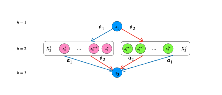
Figure 5: Lower bound construction in Theorem G.1. The blue arrows represent the transitions under the action $\mathfrak{a}_{1}$, and the red arrows represent the transitions under the action $\mathfrak{a}_{2}$. In the middle layer, the arrows to the blocks $\mathcal{X}_{2}^{1}$ and $\mathcal{X}_{2}^{2}$ denote uniform transitions to the states within those blocks.

To avoid redundancy, we only provide an informal construction of the lower bound here. A formal lower bound construction can be obtained by following arguments similar to that in Appendix C.

Proof of Theorem G.1. Let $N$ be a positive integer, and consider a state space $\mathcal{X}=\mathcal{X}_{1}\cup\mathcal{X}_{2}\cup\mathcal{X}_{3}$ where $\mathcal{X}_{1}=\{{x}_{1}\}$, $\mathcal{X}_{3}=\{{x}_{3}\}$ and $\mathcal{X}_{2}$ is of size $4N^{2}$. Consider a partition $\phi$ of $\mathcal{X}_{2}$ that divides it into two parts $\mathcal{X}_{2}^{1}$ and $\mathcal{X}_{2}^{2}$, each of size $2N^{2}$. For any such partition $\phi$, we define two MDPs $M^{\scriptscriptstyle(1)}$ and $M^{\scriptscriptstyle(2)}$, where the $M_{\phi}^{\scriptscriptstyle(i)}=MDP(\mathcal{X},\mathcal{A},H,T^{\scriptscriptstyle(i)},r^{\scriptscriptstyle(i)},\rho)$ is defined such that (this construction can be viewed in Figure 5):

1. Horizon $H=3$, action space $\mathcal{A}=\{\mathfrak{a}_{1},\mathfrak{a}_{2}\}$, and initial distribution $\rho=\delta_{{x}_{1}}(\cdot)$.

2. Transition dynamics $T^{\scriptscriptstyle(i)}$ is defined such that $T^{\scriptscriptstyle(i)}(\cdot\mid{x}_{2})=\delta_{{x}_{3}}(\cdot)$ for any ${x}_{2}\in\mathcal{X}_{2}$, and

   $$T^{\scriptscriptstyle(i)}(\cdot\mid{x}_{1},{a})=\begin{cases}\mathrm{Uniform}(\mathcal{X}_{2}^{1})&\text{if}\quad{a}=\mathfrak{a}_{1},\\ \mathrm{Uniform}(\mathcal{X}_{2}^{2})&\text{if}\quad{a}=\mathfrak{a}_{2}.\end{cases}$$

3. Reward function is defined for any ${a}\in\{\mathfrak{a}_{1},\mathfrak{a}_{2}\}$,

   $$r^{\scriptscriptstyle(i)}({x},{a})=\begin{cases}0&\text{if}\quad{x}={x}_{1},\\ 1&\text{if}\quad{x}\in\mathcal{X}^{\scriptscriptstyle(i)}_{2},\\ 0&\text{otherwise}.\end{cases}$$

We thus define the class $\mathcal{M}$ as

$$\mathcal{M}=\bigcup_{\phi\in\Phi}(M^{\scriptscriptstyle(1)}_{\phi},M^{\scriptscriptstyle(2)}_{\phi}),$$

where $\Phi$ denotes the set of all feasible partitions for $\mathcal{X}_{2}$ into $\mathcal{X}_{2}^{1}$ and $\mathcal{X}_{2}^{2}$ of the same size, and satisfies $\lvert\Phi\rvert=2^{O(N\log(N))}$.

We further define the evaluation policy ${\pi_{\mathrm{e}}}$ and ${\pi_{b}}$ such that for all ${x}\in\mathcal{X}$,

$${\pi_{\mathrm{e}}}({x})=\delta_{\mathfrak{a}_{1}}(\cdot),\qquad\text{and}\qquad{\pi_{b}}({x})=\mathrm{Uniform}(\{\mathfrak{a}_{1},\mathfrak{a}_{2}\}).$$

Then for any $M\in\cup_{\phi\in\Phi}\mathcal{M}^{\scriptscriptstyle(1)}$, we have $V^{\pi_{\mathrm{e}}}(\rho;M)=1$ and for any $M\in\cup_{\phi\in\Phi}\mathcal{M}^{\scriptscriptstyle(2)}$, we have $V^{\pi_{\mathrm{e}}}(\rho;M)=0$. Hence if the algorithm cannot tell whether $M\in\cup_{\phi\in\Phi}\mathcal{M}^{\scriptscriptstyle(2)}$ or $M\in\cup_{\phi\in\Phi}\mathcal{M}^{\scriptscriptstyle(2)}$, then the algorithm must fail to output $\nicefrac{{1}}{{2}}$-accurate estimation in at least one case among $\mathcal{M}$.

The key intuition behind the proof is that given some dataset $\mathcal{D}_{h}=\{({x}_{h},{a}_{h},r_{h},{x}_{h+1})\}$, the learner can not identify which states belong to $\mathcal{X}_{2}^{1}$ vs $\mathcal{X}_{2}^{2}$ in the second layer. Since, the reward model depends on whether ${x}\in\mathcal{X}_{2}^{1}$ or ${x}\in\mathcal{X}_{2}^{2}$, inability to identify the partition $\phi$ which split $\mathcal{X}$ into $\mathcal{X}_{2}^{1}$ and $\mathcal{X}_{2}^{2}$, will lead to an error in evaluating $V^{{\pi_{\mathrm{e}}}}(\rho;M)$ with probability $\nicefrac{{1}}{{2}}$ since we consider $\Phi$ to be the set of all possible partitions of equal size.

To see the above, note that for any $M\in\mathcal{M}$, the marginal occupancy measure at layer $2$ is

$$d_{2}^{\pi_{b}}(\cdot;M)=\mathrm{Uniform}(\mathcal{X}_{2}\times\{\mathfrak{a}_{1},\mathfrak{a}_{2}\}).$$

Hence, samples $({x}_{2},{a}_{2},r_{2},{x}_{3})$ where ${x}_{2}\in\mathcal{X}_{2}$ cannot provide useful any information unless we know whether ${x}_{2}\in\mathcal{X}_{2}^{1}$ or $\mathcal{X}_{2}^{2}$. However, while collecting admissible samples of the second layer, the distribution we samples from is $d^{\pi_{b}}_{2}(\cdot;M)$, i.e. $\mathrm{Uniform}(\mathcal{X}_{2})$, which reveals no information on $\mathcal{X}_{2}^{1}$ and $\mathcal{X}_{2}^{2}$ unless some state ${x}_{2}$ appears both in samples $({x}_{1},a_{1},r_{1},{x}_{2})$ and $({x}_{2},a_{2},r_{2})$. According to our choice of $N$, this happens with probability at most

$$1-\prod_{i=1}^{2N}\left(1-\frac{2N}{4N^{2}}\right)^{N}\leq\frac{1}{2}.$$

Hence any algorithm must fail to output $\nicefrac{{1}}{{2}}$-accurate estimation of $V^{\pi_{\mathrm{e}}}(\rho;M)$ in at least one $M\in\mathcal{M}$ with probability at least $\nicefrac{{1}}{{2}}$. $\blacksquare$

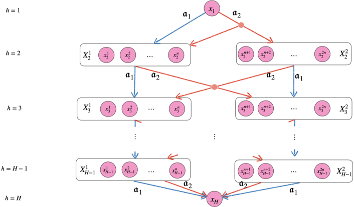
Figure 6: Lower bound construction in Theorem G.2. The blue arrows represent the transitions under the action $\mathfrak{a}_{1}$, and the red arrows represent the transitions under the action $\mathfrak{a}_{2}$. In layers for $h=2$ to $H-1$, the arrows to the blocks $\mathcal{X}_{h}^{1}$ and $\mathcal{X}_{h}^{2}$ denote uniform transitions to the states within those blocks.

Proof of Theorem G.2. Let $N=2^{H}$ and consider a state space $\mathcal{X}=\cup_{h=1}^{H}\mathcal{X}_{h}$ where $\mathcal{X}_{1}=\{{x}_{1}\}$ and $\mathcal{X}_{2},\cdots,\mathcal{X}_{H}$ are of size $4N^{2}$ each. Consider $\phi$ to be a partition of $\mathcal{X}_{2},\mathcal{X}_{3},\cdots,\mathcal{X}_{H}$ that divides each $\mathcal{X}_{h}$ ($2\leq h\leq H$) into two parts $\mathcal{X}_{h}^{1}$ and $\mathcal{X}_{h}^{2}$, each of size $2N^{2}$. For any such $\phi$, we define two MDPs $M^{\scriptscriptstyle(1)}$ and $M^{\scriptscriptstyle(2)}$, where the $M_{\phi}^{\scriptscriptstyle(i)}=MDP(\mathcal{X},\mathcal{A},H,T^{\scriptscriptstyle(i)},r^{\scriptscriptstyle(i)},\rho)$ is defined such that (this construction can be viewed in Figure 6):

1. Horizon $H$, action space $\mathcal{A}=\{\mathfrak{a}_{1},\mathfrak{a}_{2}\}$, and initial distribution $\rho=\delta({x}_{1})$.

2. Transition dynamics $T^{\scriptscriptstyle(i)}:\mathcal{X}_{h}\times\mathcal{A}\mapsto\mathcal{X}_{h+1}$ is defined such that

   $$T^{\scriptscriptstyle(i)}(\cdot\mid{x}_{1},{a})=\begin{cases}\mathrm{Uniform}(\mathcal{X}_{2}^{1})&\text{if}\quad{a}=\mathfrak{a}_{1},\\ \mathrm{Uniform}(\mathcal{X}_{2}^{1}\cup\mathcal{X}_{2}^{2})&\text{if}\quad{a}=\mathfrak{a}_{2},\end{cases}$$

   and for ${x}\in\mathcal{X}_{h}^{1}$ with $h\in[H]$,

   $$T^{\scriptscriptstyle(i)}(\cdot\mid{x},{a})=\begin{cases}\mathrm{Uniform}(\mathcal{X}_{2}^{1})&\text{if}\quad{a}=\mathfrak{a}_{1},\\ \mathrm{Uniform}(\mathcal{X}_{2}^{1}\cup\mathcal{X}_{2}^{2})&\text{if}\quad{a}=\mathfrak{a}_{2},\end{cases}$$

   for ${x}\in\mathcal{X}_{h}^{2}$ with $h\in[H]$,

   $$T^{\scriptscriptstyle(i)}(\cdot\mid{x},{a})=\begin{cases}\mathrm{Uniform}(\mathcal{X}_{2}^{2})&\text{if}\quad{a}=\mathfrak{a}_{1},\\ \mathrm{Uniform}(\mathcal{X}_{2}^{1}\cup\mathcal{X}_{2}^{2})&\text{if}\quad{a}=\mathfrak{a}_{2}.\end{cases}$$

3. Reward function: for any ${a}\in\{\mathfrak{a}_{1},\mathfrak{a}_{2}\}$,

   $$r^{\scriptscriptstyle(i)}({x},a)=\begin{cases}1&\text{if}\quad{x}\in\mathcal{X}^{\scriptscriptstyle(i)}_{H},\\ 0&\text{otherwise}.\end{cases}$$

We thus define the class $\mathcal{M}$ as

$$\mathcal{M}=\bigcup_{\phi\in\Phi}(M^{\scriptscriptstyle(1)}_{\phi},M^{\scriptscriptstyle(2)}_{\phi}),$$

where $\Phi$ denotes the set of all feasible partitions for $\mathcal{X}_{2},\cdots,\mathcal{X}_{H}$ into $\mathcal{X}_{h}^{1}$ and $\mathcal{X}_{h}^{2}$ of the same size. We further define the evaluation policy ${\pi_{\mathrm{e}}}$ and ${\pi_{b}}$ such that for all ${x}\in\mathcal{X}$,

$${\pi_{\mathrm{e}}}({x})=\delta_{\mathfrak{a}_{1}}(\cdot),\qquad\text{and}\qquad{\pi_{b}}({x})=\mathrm{Uniform}(\{\mathfrak{a}_{1},\mathfrak{a}_{2}\}).$$

For any MDP $M\in\mathcal{M}$, we observe that the occupancy measure $d_{h}^{\pi_{b}}(\cdot;M)$ is

$$d_{h}^{\pi_{b}}(\cdot;M)=\mathrm{Uniform}(\mathcal{X}_{h}\times\mathcal{A}).$$

Hence it is easy to verify that the strong coverability coefficient? of any instances in $\mathcal{M}$ is upper bounded by $4$. Additionally, we also have for any MDP $M\in\bigcup_{\phi\in\Phi}M_{\phi}^{\scriptscriptstyle(1)}$, $V^{\pi_{\mathrm{e}}}(\rho;M)=1$ and for any $M\in\bigcup_{\phi\in\Phi}M_{\phi}^{\scriptscriptstyle(1)}$, $V^{\pi_{\mathrm{e}}}(\rho;M)=0$.

The only way to tell whether a case $M\in\bigcup_{\phi\in\Phi}M_{\phi}^{\scriptscriptstyle(1)}$ or $M\in\bigcup_{\phi\in\Phi}M_{\phi}^{\scriptscriptstyle(2)}$ is through the reward function in the last layer. However, if action $\mathfrak{a}_{2}$ is taken in any step within the whole trajectory, the last layer distribution will be $\mathrm{Uniform}(\mathcal{X}_{H})$, which will induce the same reward distribution no matter the MDP is $M_{\phi}^{\scriptscriptstyle(1)}$ or $M_{\phi}^{\scriptscriptstyle(2)}$.

Hence as long as none of the trajectory collected takes only action $1$ among the trajectory, the learner will fail to output $\nicefrac{{1}}{{2}}$-accurate estimation in at least one MDP in $\mathcal{M}$ with probability at least $\nicefrac{{1}}{{2}}$. And using $o(2^{H})$ trajectories, the learner will fail to output $\nicefrac{{1}}{{2}}$-accurate estimation in at least one MDP in $\mathcal{M}$ with probability at least $\nicefrac{{1}}{{2}}-o(2^{H})\cdot\nicefrac{{1}}{{2^{H}}}\geq\nicefrac{{1}}{{4}}$. $\blacksquare$

References

- Agarwal et al. (2019) Alekh Agarwal, Nan Jiang, Sham M Kakade, and Wen Sun. Reinforcement learning: Theory and algorithms. CS Dept., UW Seattle, Seattle, WA, USA, Tech. Rep, 32, 2019.
- Amortila et al. (2020) Philip Amortila, Nan Jiang, and Tengyang Xie. A variant of the wang-foster-kakade lower bound for the discounted setting. arXiv preprint arXiv:2011.01075, 2020.
- Amortila et al. (2024) Philip Amortila, Dylan J Foster, Nan Jiang, Ayush Sekhari, and Tengyang Xie. Harnessing density ratios for online reinforcement learning. arXiv preprint arXiv:2401.09681, 2024.
- Antos et al. (2008) András Antos, Csaba Szepesvári, and Rémi Munos. Learning near-optimal policies with bellman-residual minimization based fitted policy iteration and a single sample path. Machine Learning, 71:89–129, 2008.
- Chen and Jiang (2019) Jinglin Chen and Nan Jiang. Information-theoretic considerations in batch reinforcement learning. In International Conference on Machine Learning, pages 1042–1051. PMLR, 2019.
- Chen and Jiang (2022) Jinglin Chen and Nan Jiang. Offline reinforcement learning under value and density-ratio realizability: the power of gaps. In Uncertainty in Artificial Intelligence, pages 378–388. PMLR, 2022.
- Du et al. (2019) Simon Du, Akshay Krishnamurthy, Nan Jiang, Alekh Agarwal, Miroslav Dudik, and John Langford. Provably efficient rl with rich observations via latent state decoding. In International Conference on Machine Learning, pages 1665–1674. PMLR, 2019.
- Du et al. (2021) Simon Du, Sham Kakade, Jason Lee, Shachar Lovett, Gaurav Mahajan, Wen Sun, and Ruosong Wang. Bilinear classes: A structural framework for provable generalization in rl. In International Conference on Machine Learning, pages 2826–2836. PMLR, 2021.
- Foster et al. (2022) Dylan J Foster, Akshay Krishnamurthy, David Simchi-Levi, and Yunzong Xu. Offline reinforcement learning: Fundamental barriers for value function approximation. In Conference on Learning Theory, pages 3489–3489. PMLR, 2022.
- Hoeffding (1994) Wassily Hoeffding. Probability inequalities for sums of bounded random variables. The collected works of Wassily Hoeffding, pages 409–426, 1994.
- Huang et al. (2023) Audrey Huang, Jinglin Chen, and Nan Jiang. Reinforcement learning in low-rank mdps with density features. arXiv preprint arXiv:2302.02252, 2023.
- Huang and Jiang (2022) Jiawei Huang and Nan Jiang. On the convergence rate of off-policy policy optimization methods with density-ratio correction. In International Conference on Artificial Intelligence and Statistics, pages 2658–2705. PMLR, 2022.
- Jia et al. (2024) Zeyu Jia, Gene Li, Alexander Rakhlin, Ayush Sekhari, and Nati Srebro. When is agnostic reinforcement learning statistically tractable? Advances in Neural Information Processing Systems, 36, 2024.
- Jiang (2021) Nan Jiang. Batch value-function tournament. YouTube, 2021. Available at https://www.youtube.com/watch?v=IhOfTCY-oMg.
- Jiang et al. (2017) Nan Jiang, Akshay Krishnamurthy, Alekh Agarwal, John Langford, and Robert E Schapire. Contextual decision processes with low bellman rank are pac-learnable. In International Conference on Machine Learning, pages 1704–1713. PMLR, 2017.
- Jin et al. (2021) Chi Jin, Qinghua Liu, and Sobhan Miryoosefi. Bellman eluder dimension: New rich classes of rl problems, and sample-efficient algorithms. Advances in neural information processing systems, 34:13406–13418, 2021.
- Kearns et al. (1999) Michael Kearns, Yishay Mansour, and Andrew Ng. Approximate planning in large pomdps via reusable trajectories. Advances in Neural Information Processing Systems, 12, 1999.
- Krishnamurthy et al. (2016) Akshay Krishnamurthy, Alekh Agarwal, and John Langford. Pac reinforcement learning with rich observations. Advances in Neural Information Processing Systems, 29, 2016.
- Liu et al. (2018) Qiang Liu, Lihong Li, Ziyang Tang, and Dengyong Zhou. Breaking the curse of horizon: Infinite-horizon off-policy estimation. Advances in neural information processing systems, 31, 2018.
- Mhammedi et al. (2023) Zakaria Mhammedi, Dylan J Foster, and Alexander Rakhlin. Representation learning with multi-step inverse kinematics: An efficient and optimal approach to rich-observation rl. arXiv preprint arXiv:2304.05889, 2023.
- Misra et al. (2020) Dipendra Misra, Mikael Henaff, Akshay Krishnamurthy, and John Langford. Kinematic state abstraction and provably efficient rich-observation reinforcement learning. In International conference on machine learning, pages 6961–6971. PMLR, 2020.
- Munos (2003) Rémi Munos. Error bounds for approximate policy iteration. In ICML, volume 3, pages 560–567. Citeseer, 2003.
- Munos and Szepesvári (2008) Rémi Munos and Csaba Szepesvári. Finite-time bounds for fitted value iteration. Journal of Machine Learning Research, 9(5), 2008.
- Ozdaglar et al. (2023) Asuman E Ozdaglar, Sarath Pattathil, Jiawei Zhang, and Kaiqing Zhang. Revisiting the linear-programming framework for offline rl with general function approximation. In International Conference on Machine Learning, pages 26769–26791. PMLR, 2023.
- Polyanskiy and Wu (2014) Yury Polyanskiy and Yihong Wu. Lecture notes on information theory. Lecture Notes for ECE563 (UIUC) and, 6(2012-2016):7, 2014.
- Rashidinejad et al. (2022) Paria Rashidinejad, Hanlin Zhu, Kunhe Yang, Stuart Russell, and Jiantao Jiao. Optimal conservative offline rl with general function approximation via augmented lagrangian. arXiv preprint arXiv:2211.00716, 2022.
- Sekhari et al. (2021) Ayush Sekhari, Christoph Dann, Mehryar Mohri, Yishay Mansour, and Karthik Sridharan. Agnostic reinforcement learning with low-rank mdps and rich observations. Advances in Neural Information Processing Systems, 34:19033–19045, 2021.
- Uehara and Sun (2021) Masatoshi Uehara and Wen Sun. Pessimistic model-based offline reinforcement learning under partial coverage. arXiv preprint arXiv:2107.06226, 2021.
- Uehara et al. (2020) Masatoshi Uehara, Jiawei Huang, and Nan Jiang. Minimax weight and q-function learning for off-policy evaluation. In International Conference on Machine Learning, pages 9659–9668. PMLR, 2020.
- Uehara et al. (2021) Masatoshi Uehara, Masaaki Imaizumi, Nan Jiang, Nathan Kallus, Wen Sun, and Tengyang Xie. Finite sample analysis of minimax offline reinforcement learning: Completeness, fast rates and first-order efficiency. arXiv preprint arXiv:2102.02981, 2021.
- Wang et al. (2020) Ruosong Wang, Dean P Foster, and Sham M Kakade. What are the statistical limits of offline rl with linear function approximation? arXiv preprint arXiv:2010.11895, 2020.
- Xie and Jiang (2020) Tengyang Xie and Nan Jiang. Q* approximation schemes for batch reinforcement learning: A theoretical comparison. In Conference on Uncertainty in Artificial Intelligence, pages 550–559. PMLR, 2020.
- Xie and Jiang (2021) Tengyang Xie and Nan Jiang. Batch value-function approximation with only realizability. In International Conference on Machine Learning, pages 11404–11413. PMLR, 2021.
- Xie et al. (2021) Tengyang Xie, Ching-An Cheng, Nan Jiang, Paul Mineiro, and Alekh Agarwal. Bellman-consistent pessimism for offline reinforcement learning. Advances in neural information processing systems, 34:6683–6694, 2021.
- Xie et al. (2022) Tengyang Xie, Dylan J Foster, Yu Bai, Nan Jiang, and Sham M Kakade. The role of coverage in online reinforcement learning. arXiv preprint arXiv:2210.04157, 2022.
- Zanette (2021) Andrea Zanette. Exponential lower bounds for batch reinforcement learning: Batch rl can be exponentially harder than online rl. In International Conference on Machine Learning, pages 12287–12297. PMLR, 2021.
- Zanette (2023) Andrea Zanette. When is realizability sufficient for off-policy reinforcement learning? In International Conference on Machine Learning, pages 40637–40668. PMLR, 2023.
- Zanette et al. (2020) Andrea Zanette, Alessandro Lazaric, Mykel Kochenderfer, and Emma Brunskill. Learning near optimal policies with low inherent bellman error. In International Conference on Machine Learning, pages 10978–10989. PMLR, 2020.
- Zhan et al. (2022) Wenhao Zhan, Baihe Huang, Audrey Huang, Nan Jiang, and Jason Lee. Offline reinforcement learning with realizability and single-policy concentrability. In Conference on Learning Theory, pages 2730–2775. PMLR, 2022.
- Zhang et al. (2022) Xuezhou Zhang, Yuda Song, Masatoshi Uehara, Mengdi Wang, Alekh Agarwal, and Wen Sun. Efficient reinforcement learning in block mdps: A model-free representation learning approach. In International Conference on Machine Learning, pages 26517–26547. PMLR, 2022.