GGDMiner - Discovery of Graph Generating Dependencies for Graph Data Profiling

Abstract.

With the increasing use of graph-structured data, there is also increasing interest in investigating graph data dependencies and their applications, e.g., in graph data profiling. Graph Generating Dependencies (GGDs) are a class of dependencies for property graphs that can express the relation between different graph patterns and constraints based on their attribute similarities. Rich syntax and semantics of GGDs make them a good candidate for graph data profiling. Nonetheless, GGDs are difficult to define manually, especially when there are no data experts available. In this paper, we propose GGDMiner, a framework for discovering approximate GGDs from graph data automatically, with the intention of profiling graph data through GGDs for the user. GGDMiner has three main steps: (1) pre-processing, (2) candidate generation, and, (3) GGD extraction. To optimize memory consumption and execution time, GGDMiner uses a factorized representation of each discovered graph pattern, called Answer Graph. Our results show that the discovered set of GGDs can give an overview about the input graph, both schema level information and also correlations between the graph patterns and attributes.

PVLDB Artifact Availability:
The source code, data, and/or other artifacts have been made available at %%␣The␣following␣content␣must␣be␣adapted␣for␣the␣final␣version%****␣main.tex␣Line␣25␣****%paper-specific%\newcommand\vldbdoi{XX.XX/XXX.XX}%\newcommand\vldbpages{XXX-XXX}%issue-specific%\newcommand\vldbvolume{14}%\newcommand\vldbissue{1}%\newcommand\vldbyear{2023}%should␣be␣fine␣as␣it␣is%\newcommand\vldbauthors{\authors}%\newcommand\vldbtitle{\shorttitle}%leave␣empty␣if␣no␣availability␣url␣should␣be␣sethttps://github.com/laricsh/ggdminer.

1. Introduction

Data dependencies can be understood as constraints imposed on a dataset that can be used to aid in general understanding of the data  (Liu et al., 2012; Kruse and Naumann, 2018; Abedjan et al., 2018). Consider a relation containing information about individuals, such as their ID number, name, street, city, and postal code. If there is a functional dependency (FD) defined as “street, city” $\rightarrow$ “postal code”, we can infer that individuals who live on the same street and city will have the same postal code. This particular FD helps data scientists understand the correlation of the postal code value to the street and city names.

When dealing with graph data, information about topology and attributes of the nodes/edges is important. The property graph data model (see formal definition in (Bonifati et al., 2018)) is an emerging standard in the industry, and consequently, there is an interest in developing and researching data dependencies as tools for data profiling.

Graph Generating Dependencies (GGDs) (Shimomura et al., 2020) is a class of dependencies proposed for property graphs that can express that for every homomorphic match of a source graph pattern, there should exist a homomorphic match of a (possibly) different target graph pattern. Informally, GGDs can express constraints between two (possibly) different graph patterns and the similarity of the properties of its nodes and edges (see formal definition in Section 3). GGDs introduce a new expressive power needed to capture constraints that enforce the existence of a node, edge, or a new graph pattern and give information about correlated graph patterns. The expressive power of GGDs is needed in property graphs since relationships are first-class citizens in this data model and correlation of different graph patterns can naturally arise.

GGDs can fully capture tuple-generating dependencies (tgds) compared to previously proposed dependencies for property graph, e.g. Graph Functional Dependencies (GFDs) and Graph Entity Dependencies (GEDs) (Fan and Lu, 2019), that generalize equality-generating dependencies and, cannot express a GGD. Other novelties of GGDs include (Shimomura et al., 2020, 2022): (i) can express constraints on edge attributes (not considered in GFDs and GEDs) and, (2) can express constraints on node and edge attributes according to their similarity.

The expressive power of GGDs gives deep information about correlations of different graph patterns and their properties. Consider the GGDs in Figure 1 in the context of a publication network.

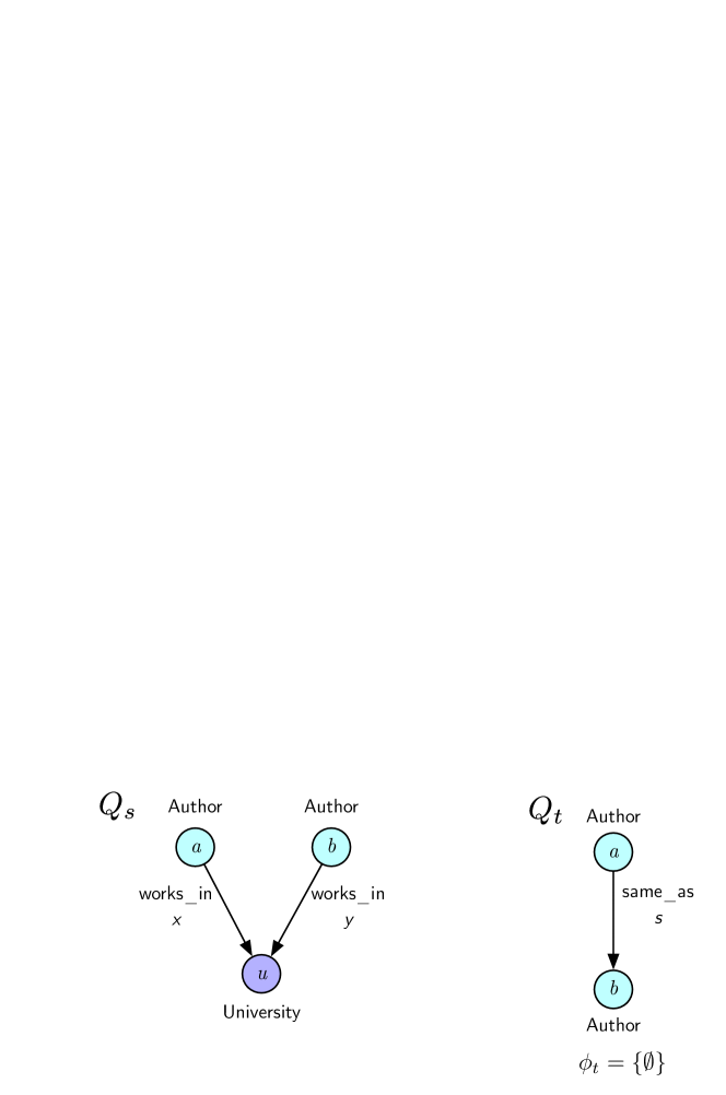
Figure 1. Example GGD

Example 0.

GGD1 expresses a constraint on the existence of a relation to another vertex. For every author who has participated in a project and authored a paper in which the paper funding grant number is similar to the project number then there should exist a Report node related to the Project and which cites the Paper.

GGD1 is an example of a tuple-generating dependency (tgd) in graph data as we are enforcing the existence of the nodes Report and the edges labeled “cites” and “from”.

Example 0.

GGD2 expresses a constraint on the attributes of a graph pattern. For every paper written by an author that has an edge to a Journal indicating publication and where the paper venue name and the journal name are similar, there should exist an edge connecting the node Paper to the Journal labeled “appeared_in” and the journal topics are similar to the paper keywords.

GGD2 gives information about how related a Paper connected to a Journal are in terms of their attributes, as whenever this dependency holds it means that the paper venue name and the journal name are similar, their topics are similar and there is an author that is connected to these two entities. GGDs can also help analysts to understand in what conditions two entities can be considered the same and express entity matching rules. Observe also that GGDs can also give information about the edge attributes of a graph pattern.

Example 0.

GGD3 expresses entity matching rules. Whenever two authors have similar names and surnames and work in the same university with a similar starting date then it means they are the same author. This should be indicated in the data by a “same_as” labeled edge.

All three of these GGDs not only help data scientists to understand the underlying relations between the nodes/edges and their attributes in the property graph but also can be used by data engineers for managing the graph. To the best of our knowledge, GGD is the only formalism that can fully capture tgds and similarity constraints for property graphs. GGDs can also express constraints on the edge attributes of the graph patterns which was not considered in previously proposed classes of dependencies.

Given these examples, it is clear that GGDs can express interesting information about the graph and be used for graph data. However, manually defining GGDs is time consuming and requires the knowledge of a data expert, therefore automatic discovery methods should be investigated.

The task of automatic discovery of GGDs is even more challenging compared to other classes of dependencies for property graphs that are defined over a single graph pattern (Fan and Lu, 2019; Fan et al., 2020, 2022). For discovering GGDs we also need to discover which graph patterns and attribute values are associated with each other.

In this paper, we propose GGDMiner, a framework for automatic discovery of Graph Generating Dependencies (GGDs) for data profiling. In particular, we focus on the task of data profiling by discovering a set of GGDs that can give an overview of the graph data. Even though GGDs have high expressive power and can be used for other applications such as rule prediction, entity resolution or data integration, the goal of GGDMiner in this paper is to discover a set of GGDs that can give initial information about the graph to the user. In ideal settings, a dataset is clean and all GGDs are fully satisfied. However, in real-world datasets this is mostly often not the case, therefore, in our work we focus on discovery of GGDs that holds for most of the data with a certain degree of inconsistency. We call such GGDs as approximate GGDs.

The GGDMiner framework consists of three main steps: (1) Pre-processing - this step serves as the preparation for the following steps in this method. This step includes sampling the graph according to the parts of the graph the user is most interested in and building indexes to assist in the process of discovering the similarity constraints in the next step. (2) Candidate Generation - in this step, we build a lattice to generate graph patterns and differential constraints that might be a source or target of a GGD. (3) GGD Extraction - In this step, we proposed a candidate index that verifies which candidates generated in the previous step can be paired to form a GGD that is interesting for describing the graph data. We give more details about the general framework and each step in Section 5.

To scale to more complex graphs, in GGDMiner we use a factorized representation of each candidate called Answer Graph (Abul-Basher et al., 2021). The answer graph was previously proposed for evaluating graph pattern queries and to the best of our knowledge our work is the first time answer graphs is used in the scenario of discovery of constraints. The factorised representation of answer graph allows us to operate on the matches of each graph pattern without defactorizing it to a table-like representation.

The goal of GGDMiner is to provide a baseline solution for discovery of GGDs with clear a step-by-step approach leveraging state of the art pattern mining algorithms in combination with our novel approach based on Answer Graph, a graph pattern query optimization technique, to represent and operate on the graph pattern matches. The use of answer graph in this framework opens a discussion on how optimization techniques for graph pattern queries can be used in discovery of graph data dependencies combined with pattern mining techniques. In our work, we show how the use of the answer graph has greatly improved memory consumption and execution time in GGDMiner. We also show how the discovered GGDs can describe information about a graph dataset to the user while providing excellent coverage.

The rest of the paper is structured as follows. In Section 2, we present related work on the discovery of graph dependencies. In Section 3, we present an overview of the GGD definition. Section 4 presents proposed measures used for discovering GGDs for data profiling and the formal problem definition. In Section 5, we discuss details of each step of the framework and, in Section 6, we present our experimental analysis and results.

2. Related Work

We place this work in the context of the following topics: (1) dependency discovery algorithms on relational data, (2) graph data dependency discovery algorithms, and, (3) frequent subgraph mining algorithms.

Relational Data Dependency Discovery

- Functional dependencies (FDs) are the arguably most used type of dependencies used in relational data. According to (Liu et al., 2012) there are mainly two approaches for the discovery of FDs: (1) top-down algorithms, also called column-based algorithms and, (2) bottom-up methods, also called row-based algorithms. These two types of approaches were also used for discovery of other types of dependencies such as Conditional Functional Dependencies (CFDs) (Fan et al., 2011), Differential Dependencies (DDs) (Kwashie et al., 2015; Song and Chen, 2011), Matching Dependencies (MDs) (Schirmer et al., 2020) and Denial Constraints (DCs) (Pena et al., 2019). A common way to represent the dependency candidates is through a lattice. How to build and traverse the lattice and the pruning techniques can vary according to the type of dependency the algorithm was proposed for (see (Liu et al., 2012; Kruse and Naumann, 2018; Papenbrock et al., 2015; Dürsch et al., 2019) for more details).

Graph Data Dependency Discovery

- Graph dependencies add the challenge of discovering information about the topology as well. The work by  (Alipourlangouri and Chiang, 2022) builds a graph that represents a summary of the topology of the input data graph, this summary is then used to create a lattice of candidate keys which is traversed and pruned to mine the resulting graph keys. In the paper  (Kwashie et al., 2019) the authors propose a lattice-based algorithm for discovering Graph Differential Dependencies (GDDs) for entity resolution. In  (Fan et al., 2020), the authors proposed a parallel algorithm for discovering Graph Functional Dependencies (GFDs). Starting from a single node pattern, this algorithm is based on two main processes: (1) vertically spawning the search space to extend the graph pattern and, (2) horizontally spawning the search space to discover the dependency literals of the GFDs. The mentioned algorithms all use either a lattice or a similar strategy to explore the search space. In GGDMiner, we propose a similar strategy in the Candidate Generation step. However, for discovering GGDs this step is not enough. Different from the GFD discovery algorithm, in GGDMiner, this is just one of the steps, used only to identify which graph patterns and constraints are frequent. To discover GGDs, we introduce the candidate index to identify which of the candidates co-occur and, use an internal factorized representation of the graph pattern matches called Answer Graph (Abul-Basher et al., 2021). The candidate index and the answer graph are a novelty of GGDMiner and have not been used in a discovery algorithm before, including the GFD discovery algorithm.

Besides graph data dependency discovery algorithms, algorithms for mining graph association rules such as discovery of GPARs (Graph Pattern Association Rules) (Fan et al., 2015) and AMIE+ (Galárraga et al., 2013, 2015) have also been proposed. GPARS is a constraint of the form $Q(x,y)\rightarrow q(x,y)$ which states if there exists an isomorphism from the graph pattern $Q(x,y)$ to a subgraph of the data graph, then an edge labeled $q$ between the vertices $x$ and $y$ should exist. Similarly, AMIE+ mines association rules of the type $B_{1}\wedge B_{2}\wedge\ldots\wedge B_{n}\Rightarrow r(x,y)$ in which $r(x,y)$ is called an atom that represents a fact in the knowledge base, such as livesIn(John, New York), and $B_{n}$, $1\leq n$, are sets of atoms in the knowledge base.

Frequent subgraph mining

- Frequent subgraph mining (FSM) refers to the task of finding all isomorphic subgraphs that occur more than a designated number of times in a graph (Jiang et al., 2013). A well-known FSM algorithm is gSpan (Yan and Han, 2002). The main idea of gSpan is to map each subgraph to a canonical DFS code being able to check if two subgraphs are isomorphic if they have the same canonical DFS code and consequently check the frequency of this subgraph. The use of DFS codes proposed by gSpan was largely used in other algorithms, including state-of-the-art algorithms such as GRAMI. The GRAMI (Elseidy et al., 2014) algorithm models the frequency evaluation of each subgraph as a constraint satisfaction problem, in which at each iteration it tries to find the minimal set of subgraph appearances that are enough to evaluate its frequency. GRAMI has been extended to support variations of the FSM problem (Elseidy et al., 2014; Moussaoui et al., 2016; Nguyen et al., 2021).

For discovering GGDs we are interested in mining graph patterns that are correlated, having constraints on the nodes/edges attributes and how they can help in describing the graph data.

3. GGDs - Definition Overview

A Graph Generating Dependency (Shimomura et al., 2020) is a dependency of the type $Q_{s}[\overline{x}]\phi_{s}\rightarrow Q_{t}[\overline{x},\overline{y}]\phi_{t}$ in which $Q_{s}[\overline{x}]$ is called the source graph pattern in which $\overline{x}$ is the set of variables (nodes and edges) in the graph pattern and $\phi_{s}$ is the set of differential constraints over $\overline{x}$ and $Q_{t}[\overline{x},\overline{y}]$ is the target graph pattern which is a graph pattern that can contain variables from the source graph pattern and additional variables, $\overline{y}$ and $\phi_{t}$ is a set of differential constraints over the variables $\overline{x},\overline{y}$.

The differential constraints can be of the form: (1) $\delta(x.A,c)\leq t_{A}$, (2) $\delta(x.A_{1},x.A_{2})\leq t_{A_{1},A_{2}}$ or (3) $x=x^{\prime}$ on which $\delta$ is a user-defined function, $x.A$ refers to attribute A of the variable x, $c$ is a constant and $t_{A}$ is a user-defined threshold. The first two types of constraints refers to comparing an attribute value to a constant or another attribute and checking if it satisfies a threshold and the third type means that x and x’ are two variables that should refer to the same node or edge in the graph.

Given a property graph $G$ (Bonifati et al., 2018), we say a GGD $\sigma$ is satisfied if for all matches $h_{s}[\overline{x}]$ of the source graph pattern $Q_{s}$ in $G$ which satisfies the source differential constraints $\phi_{s}$, denoted as $h_{s}[\overline{x}]\models\phi_{s}$, there should exist a match $h_{t}[\overline{x},\overline{y}]$ in $G$ of the target graph pattern $Q_{t}$ which satisfies the target differential constraints $\phi_{t}$, denoted as $h_{t}[\overline{x},\overline{y}]\models\phi_{t}$. The name graph generating dependencies comes from the idea that if a GGD is violated (not satisfied) on graph $G$, then new nodes or edges can be generated to repair the graph (make the GGD valid), see (Shimomura et al., 2020, 2022) for details about GGDs.

In this work, we are particularly interested in Extension GGDs. Extension GGD is a GGD in which there exists at least one variable that is explicitly part of both source and and target graph patterns. Which means that the target is an explicit extension of the source. The GGDs in Figure 1 are extension GGDs. Observe that the variable “a” and “b” in GGD3 that refers to the nodes labelled “Author” is part of both source and target graph patterns.

4. GGDs for Graph Data Profiling

As highlighted in the Introduction, in GGDMiner we are interested in discovering GGDs for graph data profiling, in other words, mining a set of GGDs that can give an overview of the graph data to the user. Having such overviews is important to understand what kind of relations (both in terms of graph patterns and in terms of their attributes) frequently appear in the graph. Therefore, we assume that if something happens frequently in a dataset then it should be considered important for describing the dataset. This assumption has also been used in previous discovery algorithms  (Alipourlangouri and Chiang, 2022; Fan et al., 2020). Considering this assumption we want to discover GGDs in which both source and target components not only happen frequently in the graph indepently of each other (defined as support of source/target) but also frequently co-occur in the graph (defined as confidence of a GGD). In the following, we present our definitions of support and confidence for GGDs.

Support

- Given a GGD $Q_{s}[\overline{x}]\phi_{s}\rightarrow Q_{t}[\overline{x},\overline{y}]\phi_{t}$, we define support of the source, denoted as $supp(Q_{s}[\overline{x}]\phi_{s})$, as the number of source matches in the graph $G$ that satisfies the source constraints, denoted as $|h_{s}[\overline{x}]\models\phi_{s}|$. Respectively, we define support of the target defined as $supp(Q_{t}[\overline{x}\overline{y}]\phi_{t})$ as the number of target matches in the graph $G$ that satisfies the target constraints, denoted as $|h_{t}[\overline{x}\overline{y}]\models\phi_{t}|$.

Confidence

- We define the confidence of GGDs according to its semantics, a GGD is said to be validated if for all matches of the source there exists a match of the target. Therefore, considering $\alpha=Q_{\alpha}[\overline{x}]\phi_{\alpha}$ and $\beta=Q_{\beta}[\overline{y}]\phi_{\beta}$ and there exists at least one variable $a\in\overline{x}$ in $\alpha$ which can match to the same nodes/edges to a variable $b\in\overline{y}$ in $\beta$ then the confidence of the GGD

$$conf(\alpha\rightarrow\beta)=\frac{|Validated(\alpha\rightarrow\beta)|}{supp(\alpha)},$$

in which $|Validated(\alpha\rightarrow\beta)|$ is the number of matches of $\alpha$ in which the possible GGD $\alpha\rightarrow\beta$ is validated (satisfied) and $supp(\alpha)$ is the total number of matches of the source side $\alpha$.

Complementary to frequency, we are interested in discovering a set of GGDs that maximizes how much we can describe about the graph data and minimize the similarity between the GGDs of the set. Since the main goal is to give an overview to the user, a set of GGDs that can describe the graph data is a set of GGDs which can give information about the biggest number of nodes and edges in the graph. To quantify how much a discovered set of GGDs describes a graph dataset, we propose the coverage measure.

Coverage

- Coverage is a measure used in previous works in the literature to define how much of the data a particular dependency can give information about. Following the semantics of the GGDs, we are mainly interested in how much the source side can give information about the data. Therefore, we define coverage of a set of GGDs $\Sigma_{G}$ as:

$$coverage(\Sigma_{G})=\frac{|\cup_{\sigma\in\Sigma_{G}}O(\sigma)|}{|G|},$$

in which $O(\sigma)$ is the set of matching nodes and edges of the source side of the GGD and $|G|$ is the total number of nodes and edges in the input graph $G$.

Following the idea that we do not want a set which contains very similar GGDs, we also define decision boundary and candidate similarity which are used during the GGDMiner to avoid very similar GGDs according to the GGD “structure” (graph pattern and differential constraints).

Decision Boundary

- The decision boundary is a tuple $<\upsilon,\kappa>$ that is defined for each attribute data type in the graph data, for example, strings, numbers, sets, dates, etc. The $\upsilon$ refers to the minimal threshold (dissimilarity) value and the $\kappa$ is the minimal difference between two threshold values. We say that a set $\phi$ of differential constraints on the same attribute and same constant values respect a decision boundary if the smallest discovered threshold $t$ of the set is bigger than $\upsilon$ and the smallest difference between all threshold of the set $\phi$ is bigger than $\kappa$. The decision boundary is used to avoid the discovery of differential constraints that are very similar and are not interesting.

Example 0.

Consider $\alpha=Q_{\alpha}[\overline{x}]\phi_{\alpha}$ and two differential constraints discovered over the string attribute name $\phi_{\alpha}=\{\delta_{\text{name}}(x.name,$ $x.surname)\leq 3$ , $\delta_{\text{name}}(x.name,x.surname)\leq 1\}$, and a decision boundary defined for string attributes as $<1.0,2.0>$ then it means that the minimal threshold to consider when discovering differential constraints is $1.0$ and the minimal difference between the thresholds of two differential constraints to be considered in the discovery algorithm is $2.0$, since all thresholds in $\phi_{\alpha}$ are at least $1$ and the smallest difference between its threshold is $2$ ($3-1=2$), then $\phi_{\alpha}$ respects the decision boundary.

Candidate Similarity

- Considering $\alpha=Q_{\alpha}[\overline{x}]\phi_{\alpha}$ and $\beta=Q_{\beta}[\overline{y}]\phi_{\beta}$, we measure the similarity between $\alpha$ and $\beta$ according to 2 aspects: (i) Graph pattern denoted as $\delta_{Q}(Q_{\alpha},Q_{\beta})$, (ii) Differential constraints, denoted as $\delta_{\phi}(\phi_{a}lpha,\phi_{\beta})$. Given these two aspects, the overall similarity $\Delta$ between $\alpha$ and $\beta$ is defined as:

$$\Delta(\alpha,\beta)=\frac{\delta_{Q}(Q_{\alpha},Q_{\beta})+\delta_{\phi}(\phi_{\alpha},\phi_{\beta})}{2},$$

in which $\delta_{Q}(Q_{\alpha},Q_{\beta})$ is the number of common edges (same edge label, source node label and target node label) and $\delta_{\phi}(\phi_{\alpha},\phi_{\beta})$ is the number of differential constraints that refer to the same attribute of the same node/edge label.

The GGD discovery problem

- Considering the coverage measure, given an input property graph $G$ and assuming that we have information about the attributes and the domain that each node/edge label has (see Figure 3), we define the GGD discovery problem for graph data profiling as follows:

Input:

Given an input property graph $G$ and support $\tau$, a set $T$ of decision boundary for each attribute domain of values that can be assigned by $\nu$, a confidence value $\epsilon$, a similarity value $\theta$ and a maximum number of edges $k$.

Output:

A set of Extension GGDs $\Sigma_{G}$ which maximizes coverage in which each GGD in $\Sigma_{G}$ has confidence bigger than $\epsilon$. And, the source and target of each GGD that has support is bigger than $\tau$.

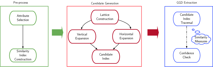
Figure 2. General Framework of the Discovery Algorithms

Besides the support $\tau$ and confidence $\epsilon$ values, we also introduce the parameter $k$ and the parameter $\theta$, in which $k$ refers to the maximum number of edges each graph pattern (source or target) in a GGD can have and, $\theta$ is a similarity threshold which defines how similar a GGD can be from another GGD from the discovered set $\Sigma_{G}$. Such parameters are introduced to reduce a drawback seen in many dependency discovery algorithms and frequent subgraph mining solution. The referred drawback is the big number of discovered dependencies that are very similar and do not aggregate information to the result. Thus, initially, we want to give an overview of the graph dataset to the user, in case the user is interested in more complex graph patterns, after seeing the initial result, the user can build up his knowledge about the entities he is most interested about. Therefore, the parameter $k$ introduces this maximum number of edges to give an initial overview of the frequent graph of the whole graph and the similarity threshold $\theta$ indicates the similarity between GGDs.

An important step in discovery algorithms is candidate generation. As already discussed in previous works in the literature (Liu et al., 2012; Abedjan et al., 2018), the number of candidate dependencies to be considered can be exponential to the number of attributes of the data. Compared to other graph dependencies, discovering GGDs has the additional challenge of discovering relations between the graph patterns and the differential constraints on its attributes, increasing even more the number of candidates.

By definition, each differential constraint on a GGD can be according to a user-defined distance measure. To reduce the scope of the candidate generation, we fix a distance measure for each attribute domain. In this paper, we use the edit distance for string values and for numerical values we use the absolute difference. We define also a set $T$ of decision boundaries. Given this problem definition, next, we present the GGDMiner framework for automatic discovery of GGDs.

5. GGDMiner Framework

The GGDMiner framework has three main steps: (1) Pre-processing; (2) Candidate Generation and (3) GGD Extraction. Figure 2 provides an overview of the framework.

Pre-processing

- This step is responsible for preparing for the mining steps (candidate generation and GGD extraction). The tasks of this step are: (1) Identifying which are possible extensions and important attributes to consider during the candidate generation and, (2) Constructing similarity indexes for the important attributes.

Candidate generation

- The candidate generation step is responsible for mining interesting graph patterns from the data and the possible differential constraints each graph pattern holds. We generate such candidates by constructing a lattice in a similar fashion to previous algorithms on data dependency discovery. The lattice construction uses two main processes: (1) Vertical expansion, which expands the lattice vertically (adds a new level) and is responsible for expanding the graph patterns and, (2) Horizontal expansion, which expands the lattice at the same level by mining the possible differential constraint a graph pattern might hold on this data. Each new graph pattern and set of differential constraints with support bigger than $\tau$ is added to the candidate index.

GGD Extraction

- The final step of the framework, this step is responsible for traversing the candidate index in order to pair the candidate graph patterns and differential constraint mined in the previous step and extract the set of GGDs in which the confidence value is above the threshold $\epsilon$. It is also during the index traversal that the similarity between the GGDs is measured.

Next, we give details of each one of these steps. We use a graph with the schema in Figure 3 as a running example throughout the section.

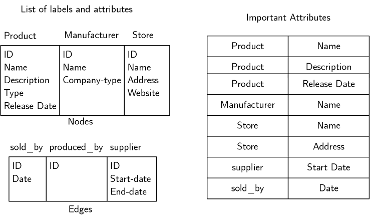
Figure 3. Example Graph Schema and Important attributes selected

5.1. Pre-processing

The pre-processing step is responsible for preparing for the mining steps. The main goal of the pre-processing step is to select node/edge labels and its attributes that have a high probability of appearing frequently on the graph (support ¿ $\tau$) and should be verified as part of a GGD candidate in the next steps of the framework.

First, given the set of labels of the graph, in this first step, we filter out labels that the number of nodes/edges is smaller than $\tau$. From this point, we consider only the labels which have a frequency bigger than $\tau$. Next, we select attribute pairs. That means, we identify which attributes of the considered labels have a high probability to appear in a differential constraint. Finally, we build auxiliary data structures that will be used on the discovery of differential constraints in the Candidate Generation step.

Selecting Attribute Pairs

In this task we select which are the attributes for each label that can be compared to each other to form differential constraints of the type $\delta_{\text{attr}}(x.attr_{1},y.attr_{2})\leq t_{x,y}$, considering that $x$ and $y$ are variable of the same graph pattern with (possibly) different labels and $attr_{1}$ and $attr_{2}$ are attributes of the same domain. Considering that we are assuming that the user have information about the attribute and domain of each label available, in case the user already knows which attributes are considered more important, this can be set manually. In case it is not set manually by the user, based on the assumption that attributes with similar values should also have semantically similar names, we select attributes which its name semantic similarity is above a user-defined threshold. We use the semantic similarity because (i) we are looking for semantic correlations between the attributes and (ii) to compare just the attribute names according to semantic similarity is faster than comparing all the actual values of the attributes (unless for all labels of nodes and edges there are more attribute names than values). See an example of selected attribute pairs in Figure 3.

Similarity Indexes

To discover differential constraints of the type $\delta_{\text{attr}}(x.attr_{1},\varrho)\leq t_{x}$, we build similarity indexes according to the domain of $x.attr_{1}$ and $\varrho$ to assist on the discovery process of such constraints in the Candidate Generation step. The attributes of each node/edge label that we use to build such indexes are either set manually or we consider only the attributes that were selected as part of a pair in the previous task. Given the set of attributes, for each one of the attributes we build a structure which groups the attribute values according to their similarity value and the threshold of its corresponding decision boundary domain, we call this structure similarity cluster.

To build a similarity cluster, we first select all values of the attribute and the minimal threshold $\upsilon$ defined for this domain of the decision boundary set $T$. Next, we execute the pass join (Li et al., 2011) algorithm, a string similarity join algorithm, with threshold $\upsilon$ to get all pairs of values that are similar according to $\upsilon$. Next, we cluster the joined pairs so that all pairs of values that were joined between each other are in the same cluster. Each one of these similarity clusters is stored temporarily to be used in the next step. We used the pass join because it is an algorithm that is easy to implement and has good memory consumption in previous comparisons to other similarity join algorithms (Jiang et al., 2014). By using a similarity join algorithm to build the clusters, we allow one attribute value to be part of multiple clusters. While this increases the number of clusters, it decreases the number of similarity comparisons during the candidate generation step, as we already have separated sets of attributes with the maximum dissimilarity of $\upsilon$ within all attribute values of this set. We explain how we use the similarity cluster with more details in Section 5.2.2 Observe Figure 5 an example of this process given a set of attributes “name”.

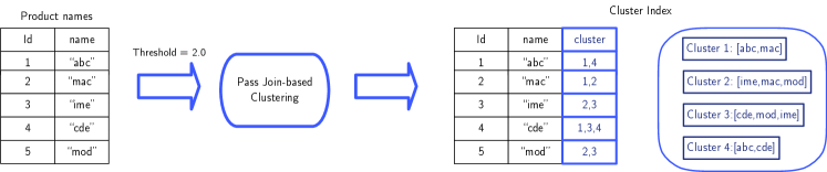
Figure 4. Similarity Clustering Index

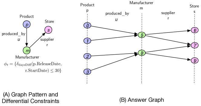
Figure 5. Answer Graph Example

5.2. Candidate Generation

In this step, we propose a lattice-based algorithm that uses a graph pattern mining algorithm and the previously built similarity indexes to generate/mine all graph patterns and respective sets of differential constraints in which the support is above $\tau$.

In GGDMiner, we use a lattice to generate the possible candidates for the source or target of a GGD. Each lattice node corresponds to a graph pattern $Q[\overline{x}]$, a set of differential constraints $\phi$ and an answer graph $E$ (Abul-Basher et al., 2021), a factorized representation of the matches of this graph pattern that satisfies the differential constraints $\phi$. Each lattice node is a candidate for the source or target of a GGD.

Answer graph

The answer graph is defined as a subset of the graph that suffices to compute the matches of a graph pattern (Abul-Basher et al., 2021). In GGDMiner, the answer graph is the intermediate representation of the matching nodes and edges of each lattice node. The use of answer graph is one of the key components of GGDMiner and it is a compact subgraph representation in which we can execute operations over the matching nodes and edges of each lattice node without needing to extract (defactorize) the full matches of the graph pattern in a table-like representation. The operations include adding new edges, filtering, calculating confidence by traversing the Answer Graph. Given a graph pattern, see the corresponding answer graph in Figure 5.

5.2.1. Lattice Construction - Discovery of Candidates

As mentioned before, each lattice node refers to a graph pattern $Q[\overline{x}]$, a set of constraints $\phi$ and its matching nodes and edges represented by an answer graph $E$. At each level of the lattice we expand the graph pattern $Q[\overline{x}]$ by one edge, we call this process vertical extension. And, on the same level of the lattice, there are graph patterns with the same number of edges but with different sets of differential constraints, we call this process horizontal expansion. We summarize the steps of the lattice construction in Algorithm 1.

Algorithm 1 Lattice Construction

1:procedure LatticeConstruction(Graph $G$, Support $\tau$, Frequent Node Labels $L_{v}$, Frequent Edge Labels $L_{e}$)

2:    Create empty lattice structure $L$

3:    Create empty Candidate Index $C$

4:    level $\leftarrow 0$

5:    for each $l_{v}\in L_{v}$ do

6:         Initialize graph pattern $Q_{l_{v}}$ with single node of label $l_{v}$ and $\phi_{l_{v}}=\{\emptyset\}$

7:         $E\leftarrow$ CreateAnswerGraph($G$, $Q_{l_{v}}$, $\phi_{l_{v}}$)

8:         L.addNode(level, $Q_{l_{v}}$, $\phi_{l_{v}}$, $E$)

9:         C.addCandidate($Q_{l_{v}}$, $\phi_{l_{v}}$, $E$)

10:         HorizontalExpansion(level, {$Q_{l_{v}}$, $\phi_{l_{v}}$, $E$}, $\tau$, L, C)

11:         for each $l_{e}\in L_{e}$ do

12:             if $l_{e}$ can expand $Q_{l_{v}}$ then

13:                 $Q_{l_{v},l_{e}}\leftarrow$ Expand $Q_{l_{v}}$ by adding edge of label $l_{e}$

14:                 level $\leftarrow$ level + 1

15:                 $E_{l_{e}}\leftarrow$ ExtendAnswerGraph($G$, $E$, $Q_{l_{v},l_{e}}$, $\emptyset$)

16:                 L.addNode(level, $Q_{l_{v},l_{e}}$, $\emptyset$, $E_{l_{e}}$)

17:                 C.addCandidate($Q_{l_{v},l_{e}}$, $\emptyset$, $E_{l_{e}}$)

18:                 HorizontalExpansion(level, {$Q_{l_{v},l_{e}}$, $\emptyset$, $E_{l_{e}}$}, $\tau$, L, C)

19:                 VerticalExpansion(level, $G$, $\tau$, $L$, $C$, { $Q_{l_{v},l_{e}}$, $\emptyset$, $E_{l_{e}}$}, $k$, $L_{e}$)

20:                 Remove $l_{e}$ from $G$ and $L_{e}$                           

Algorithm 2 Vertical Expansion

1:procedure VerticalExpansion(Level Number level, Graph $G$, Support $\tau$, Lattice $L$, Candidate Index $C$, Lattice Node to extend { $Q$, $\phi$, $E$}, Maximum number of edges $k$ , Frequent Edge Labels $L_{e}$)

2:    level $\leftarrow$ level + 1

3:    if Number of edges in $Q\geq k$ then

4:         return     

5:    fExtensions $\leftarrow$ FSMSubgraphExtension($Q$, $G$, $\tau$, $L_{e}$)

6:    for  each $Q_{ext}\in fExtensions$ do

7:         $E_{ext}$ $\leftarrow$ ExtendAnswerGraph($G$,$E$, $Q_{ext}$, $\emptyset$)

8:         L.addNode(level, $Q_{ext}$, $\emptyset$, $E_{ext}$)

9:         C.addCandidate($Q_{ext}$, $\emptyset$, $E_{ext}$)

10:         HorizontalExpansion(level, $\{Q_{ext},\emptyset,E_{ext}\}$, $\tau$, L, C)

11:         VerticalExpansion(level, $G$, $\tau$, L, C, $\{Q_{ext},\emptyset,E_{ext}\}$, $k$, $L_{e}$)     

We initialize the lattice by adding nodes with a single vertex graph pattern and an empty set of differential constraints for each vertex label of the graph $G$ which has support bigger than $\tau$. The answer graph of these nodes is initialized with the identifier (ids) of all the vertices that correspond to this label. Next, we discover the differential constraints for each one of these lattice nodes. The discovery process for the differential constraints is described in detail in Section 5.2.2.

For each one of the discovered set of differential constraints, we add another lattice node with the same graph pattern and the set of the differential constraints in the same level (in this case, first level) of the lattice.Observe level $0$ in Figure 6 which contains single-node patterns with and without differential constraints.

For each newly added lattice node in the horizontal expansion, we create a new answer graph. We filter the answer graph of the lattice node that has the same graph pattern and empty set of constraints by removing nodes and edges that do not satisfy the set of differential constraints. Finally, we apply a node burn-back on this new answer graph. The node burn-back is a procedure used in answer graph to remove any disconnected nodes and edges (for more details on the node burn-back see  (Abul-Basher et al., 2021)). For every lattice node $Q_{0}[\overline{x}]\phi_{0}$ whose support is larger than $\tau$, we add this node to a structure we call candidate index used in the final step of GGDMiner.

To expand the lattice vertically, we use a frequent subgraph mining (FSM) algorithm. At each vertical expansion, we add one edge to the graph pattern of the previous level lattice nodes. In this implementation we use the GRAMI (Elseidy et al., 2014) algorithm but it can be replaced by any other technique that can check if a graph pattern is frequent according to the support value $\tau$. The GRAMI algorithm uses gSpan to generate candidates and a CSP (Constraint Satisfaction Problem) strategy to verify the subgraph frequency. At each edge extension (right most extension in gSpan) in which the frequency is higher than $\tau$, we add a new node to the lattice containing this new extended graph pattern $Q_{1}$ and an empty set $\phi$ of differential constraints. The use of gSpan DFS (depth-first search) codes allows us to naturally organize the levels of the lattice and also quickly verify which nodes with different sets of differential constraints are the same. We also create an answer graph for this new lattice node by extending the answer graph of the parent lattice node to $Q_{1}$ (in this case, $Q_{0}$) with the matches of the edge extended. At each edge extended in the answer graph, we run a node burn-back which deletes from the answer graph all the disconnected nodes and edges that are not part anymore of this subgraph.

Next, we run a horizontal extension to discover differential constraints considering only the new variables included in the graph pattern using the new edge and new vertex that was added to the graph pattern. Similarly, for each set of differential constraints added, we add a lattice node in the same level and add all these nodes in the Candidate Index. Algorithm 2 summarizes this process and figure 6 show a figure of the lattice for our running example. This process of expanding the lattice is repeated until the number of edges in the graph pattern of the lattice node is bigger than $k$.

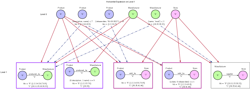
Figure 6. Level 1 of the lattice after vertical and horizontal expansion

5.2.2. Discovery of Differential Constraints

The discovery of differential constraints relies on the attribute pairs selected in the pre-processing step of this framework. Given a graph pattern $Q[[\overline{x}]]$ in which $\overline{x}$ is the set of variables, we first verify which variables have attributes considered important according to our pre-processing step. We discover differential constraints concerning only the variables (node/edge) that have attributes considered important. Thus, to avoid recalculations, at every vertical expansion of the lattice we consider only the variables that were added to the graph pattern. We take inspiration from methods for mining association rules with intervals for discovering differential constraints in GGDs. The main difference is that, in the case of differential constraints for GGDs, the intervals are the thresholds indicating how similar two attributes or an attribute and a constant are.

Given a graph pattern $Q[\overline{x}]$, its set of matches $E$, support $\tau$, and decision boundaries $T$ we first discover differential constraints of the type $\delta(x.A,cons)\leq t$ where an attribute $A$ of a variable $x$ is compared to a constant $cons$.

For each variable $x$ added to the graph pattern at the last extension, we first identify if there any attributes of $x$ in the list of important attributes of the pre-process step. If yes, we retrieve the set of values $V$ of attribute $A$ of $x$ in the set of matches $E$ and identify which clusters $C$ each value $v\in V$ is part of. Then for each identified cluster $c\in C$, if the size of $C$ is bigger than $\tau$ then it means that there is a differential constraint regarding the attribute $x.A$.

Then, given the set of values of each cluster $c$, we choose what is the best value in the cluster $c$ to be used as the constant $cons$. The idea is to choose a constant value that maximizes the support of the differential constraint as much as possible, therefore, we select the value that has the lowest average (dis)similarity to all other values in the cluster.

Given the constant value $cons$ and its (dis)similarity to all other cluster values, we execute a function called FindIntervals that will discretize these (dis)similarity values in a way that maximizes the support/frequency of each value interval, the intervals correspond to the threshold values of the discovered constraint. The discretization process also takes into consideration the decision boundary of the attribute domain, which means that the discovered constraints should be at least $\upsilon$ similar to be considered a differential constraint and the intervals discovered should have at least $\kappa$ difference between them. Any interval in which the support is higher than $\tau$ is added as a new constraint in the result set of the procedure.

Next, we execute a similar algorithm to discover a differential constraint of the type $\delta(x.A,x^{\prime}.B)\leq t$, in which a variable attribute is compared to (possibly other) variable attribute is very similar to the described algorithm. However, in this case, instead of verifying which attributes are on the list of most important attributes, we verify which attributes can be paired/compared to other attributes. Thus, since we do not have a cluster pre-built in the preprocess step, instead we use the pass join algorithm to cluster the values of each pair of attributes (same procedure as when building the similarity indexes in the pre-processing step).Then for each cluster, we discretize the (dis)similarity values in the same way as in FindIntervals, with the goal of maximizing the support of each interval. Any discovered interval in which the support is higher than $\tau$ is added to the result set.

Observe that not all attributes of each variable are in the list of important attributes and, since at each edge extension we consider only the variables that are new to this graph pattern the number of possible differential constraints is bounded and limited. We use a naive implementation for the discovery of differential constraints as our main goal in GGDMiner is to systemize the discovery of GGDs in a framework solution. Algorithms used in vertical and horizontal expansion can be substituted by other algorithms with the same output, as long as answer graph can be used to represent a lattice node.

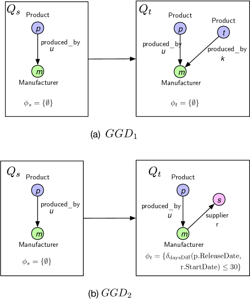
Figure 7. Examples of GGDs

5.2.3. Candidate Index

The candidate index has mainly two data structures: (1) a set $C$ of candidates that will serve as the source of the extracted GGDs and, (2) a graph-based index in which each node refers to a lattice node and each edge is how similar theses nodes are according to the similarity measure $\Delta$.

The goal of this index is twofold:(1) find the candidates that will be the source side of the extracted GGDs such that this set maximizes coverage and, (2) to find interesting target candidates that can be paired to such sources and minimize the verification of pairs of candidates that will probably not aggregate information to our final GGD set.

We use a greedy-based approach to select the set of source candidates that maximizes the coverage. Whenever a new candidate $\{Q_{l},\phi_{l},E\}$ is added to the index (line 9 and line 17 of Algorithm 1) we verify if this newly added candidate can increase the coverage of the current set. If it can increase, we verify if there is a subset $S$ of $C$ in which $\{S\}\cup\{Q_{l},\phi_{l},E)\}$ has the same coverage as $\{C\}\cup\{(Q_{l},\phi_{l},E)\}$, if there is then $\{S\}\cup\{Q_{l},\phi_{l},E)\}$ is the new set $C$. If there is not, then $\{(Q_{l},\phi_{l},E)\}$ is added to $C$. We calculate coverage by retrieving the matching nodes and edges of each candidate answer graph, and there is no need to revisit the input graph $G$.

The similarity between the candidates is what defines how interesting a possible target candidate is or not. Suppose Figure 7(a) and (b) have the same confidence value, in GGD1 source and target are very similar with just one edge difference. Compared to GGD1, GGD2 aggregates more information about the graph $G$ as it is about two different contexts of information in the graph $G$, thus GGD2 also aggregates information between the attributes of its graph patterns.

5.3. GGD Extraction

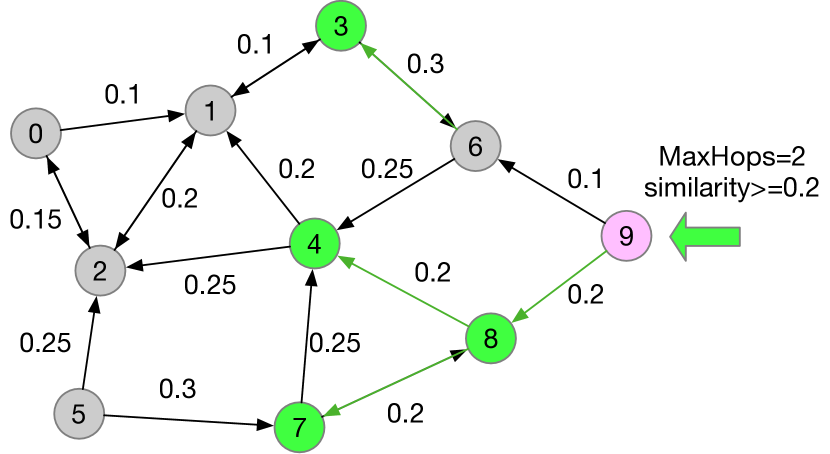
Figure 8. Extraction of possible lattice nodes which can possibly form a GGD with source lattice node 9

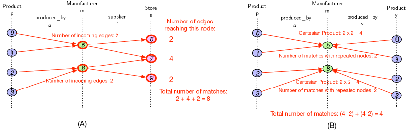
Figure 9. Calculating number of matches from answer graph for (A) a chain pattern and (B) a snowflake pattern

The last step of the GGDMiner framework is the GGD Extraction. The main goal of this step is to extract the final results from the candidate index. Given the mined graph patterns and differential constraints in the candidate index, in this step, we combine the mined candidates as possible GGDs and verify which candidates have a confidence value above the threshold $\epsilon$.

The similarity measure $\Delta$ is a symmetric measure that defines how many common edges and common differential constraints two candidates have. We use an approximate $k$-NN graph (Dong et al., 2011) as the graph-based index in the candidate index of GGDMiner. In this graph-based index, each node corresponds to a candidate and the edges correspond to their similarity according to the measure $\Delta$. We run a search algorithm on the $k$-NN graph to pair candidates which are not too similar to the point that is not interesting but still similar enough so that it is a valid GGD (confidence higher than $\epsilon$). Given a starting vertex $u$, a similarity threshold $\delta$, and a maximum number of hops $m$, we run a breadth-first search starting from vertex $u$ until it reached $m$ hops from $u$. For each node visited $n$ during this search process, if $\Delta(u,n)\geq\delta$, we add $n$ to the result set $N$ of the search. We run this search starting from each one of the vertices in the set $C$ in the candidate index. The set of pairs of the resulting $N$ set of the algorithm are the possible GGDs. Observe that by using this search method, since we have a maximum number of hops from $u$ and $u$ is a vertex in $C$, regardless of the user-defined confidence value $\epsilon$, there is a maximum number of $k{{}_{g}}^{m}$ possible candidates to evaluate if they should be paired with each $u\in C$ or not, in which $k_{g}$ is the number of neighbors $k$ in the $k$-NN graph. In Figure 9 we show the graph-based index of the Candidate Index with 10 candidates from the candidate generation step and highlight in green, the possible target candidates of the source candidate with index $9$ (in pink).

Next, for each one of these pairs, we verify if the confidence is above the threshold $\epsilon$. Since we are looking for Extension GGDs, there should exist at least one common variable in source and target. We first verify which are the possible mappings we can have from the graph pattern from $c_{1}$ to $c_{2}$ in which there is at least one variable that refers to that match the same nodes or edges in both graph patterns. If there does not exist such mapping then this pair is discarded as a possible GGD. Such verification is a hard problem as it can be translated to a problem of finding a common subgraph between both graph patterns. To simplify the computation, we use the idea of the DFS Codes used by gSpan to verify a possible mapping between both graph patterns. Then, for each one of the possible mappings, we calculate the confidence of $c_{1}\rightarrow c_{2}$. If $confidence(c_{1}\rightarrow c_{2})\geq\epsilon$, we rename the variables in $c_{2}$ according to our mapping and add $c_{1}\rightarrow c_{2}$ as a GGD to our result set $\Sigma_{G}$.

To calculate the confidence of a GGD, we first calculate the number of source matches represented by the source answer graph. This is the total number of source matches used in the confidence calculation. Next, considering the common variables between the source and target, we remove from the source answer graph matching nodes/edges that do not exist in the target answer graph. Essentially, we filter the source answer graph to have only the matching nodes and edges that are validated by the target. Then, we calculate the number of matches that is represented by this filtered answer graph, which corresponds to the number of validated matches. The method for calculating the number of nodes and edges from answer graph depends on the shape of the graph pattern. In this paper, we limited the graph patterns to the shapes shown in Figure 9. Observe in Figure 9 how we calculate the number of matches without defactorizing answer graph for these two types of shapes. Such a procedure allows us to calculate the confidence of a GGD without defactorizing (extracting the matches) the source or the target answer graph in a table-like representation and without needing to retrieve any extra information from the input graph $G$. By the end of this step, we have our final set of GGDs $\Sigma_{G}$ that describes $G$.

6. Experimental Evaluation

Dataset	Node Labels	Edge Labels	Nodes	Edges
Cordis	11	12	32K	151K
GDelt	5	2	73K	445K
DBLP	4	4	2M	810K
LDBC	8	23	430k	2M

Table 1. Datasets used in experiments

In this section, we use the real-world datasets Cordis, GDelt, DBLP and the synthetic dataset LDBC which was generated using the LDBC Social Network Benchmark Data generator (Angles et al., 2020) with scale factor $0.1$ (see Table 1) to evaluate GGDMiner. We evaluate the impact of the main user-defined parameters on execution time, coverage of discovered GGDs and, show example of GGDs discovered by GGDMiner. Due to limited space, details about the content of the datasets and its schema information are available in our repository. For all experiments, we used $\epsilon=0.7$ and $\theta=0.5$, unless when mentioned otherwise. GGDMiner was implemented using Java and deployed on an Intel Xeon machine with 3.07GHz using 128GB of RAM.

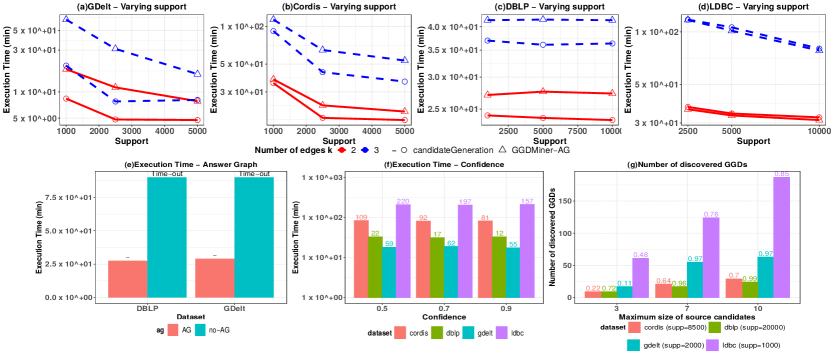
Figure 10. GGDMiner Experimental Results - Scalability and Coverage

6.1. Scalability and Coverage

Impact of discovery of graph patterns

One of the main innovations of GGDs compared to previous data dependencies is how we can express a correlation between two (possibly different) graph patterns. In this first experiment, we evaluate how the discovery of the graph patterns (Candidate Generation) and checking correlated graph patterns (GGD Extraction) affects the overall execution of GGDMiner. To make this comparison, for this experiment only, we run the GGDMiner without the differential constraint discovery, to make a fair comparison between the search time of the graph pattern mining algorithm used compared to GGDExtraction.

We evaluate the execution time of GGDMiner according to the support $\tau$ parameter and also maximum number of edges $k$ in the graph patterns, results are shown in Figure 10(a)-(d). These two parameters control the number of possible candidates of source and target the GGDMiner can have, as the smaller the value $\tau$ and bigger the $k$ the bigger the number of possible candidates of graph patterns and differential constraints to be evaluated.

When comparing, the execution time of GGDMiner to the execution of only Candidate Generation we can observe that the execution time increases in approximately $1$ order magnitude for GDelt. This is because, even though the number of candidates considered source of a GGD is limited and the number of candidates that can be considered target is also limited based on the candidate index, a pair of candidates can have multiple mappings (set common nodes or edges) and for each mapping a confidence value must be calculated, increasing the execution time. The number of different mappings can be even higher when there is an entity/node label in the graph dataset that is the main subject of that dataset and appears in most of graph patterns considered as candidates. Since we considered datasets in the context of citation networks, this occurs in all of the datasets. Considering $\tau=1000$ and $k=2$, in the GDelt dataset the FSM algorithm mined a total of $18$ graph patterns in which all of them include at least one node labelled “Article”, in the DBLP dataset all the mined graph patterns include a node labelled “Paper” of a total of $20$ mined graph pattern and, in Cordis, from the total of $31$ mined graph patterns $20$ of the mined graph patterns include a node labelled “Project” and $15$ include a node labelled “Paper”, which means that for almost every pair of candidates considered as a possible GGD in the GGD Extraction step, there will be at least one mapping to check the confidence. However, the increase for Cordis and LDBC is less accentuated. This is due to both of these datasets having a higher number of node and edge labels, and consequently checking the possible frequent subgraphs takes more time, accentuating the overall execution time compared to GDelt and DBLP.

We can also observe the difference in execution time according to parameter $k$ (maximum number of edges). In Cordis and in the LDBC dataset, given the bigger number of nodes and edge labels to be considered and evaluated as candidates in the candidate generation step, there is a bigger difference in execution time from $k=2$ to $k=3$ compared to other datasets.

Impact of Answer Graph

The Answer Graph is one of the key elements of GGDMiner. It is used to (1) represent the matches nodes and edges during the Candidate Generation step and, (2) calculate the confidence value of GGDs without having to defactorize it (extracting the list of matches). We evaluate how much Answer Graph improves the execution time and memory in GGDMiner compared to a version of GGDMiner that uses a table-like representation of each graph pattern match for confidence checking. The results are in Figure 10(e). Due to the long execution time of GGDMiner without the full use of Answer Graph we fixed a maximum execution time of 1.5 hours. Results for Cordis and LDBC were not reported as the version not using Answer Graph have run out of memory.

From the plots, we can easily identify how the use of Answer Graph improves significantly the execution time of GGDMiner even for small graph pattern such as $k=2$ in several orders of magnitude. For both datasets Cordis and GDelt, the execution time has exceeded our fixed limit while the execution time when using the Answer Graph was below the fixed limit. When using a table-like representation for the graph pattern matches it can run out of memory, this is because a single node can appear in different matches, each different row is added to the table as a match. Not using Answer Graph for checking confidence also has the extra time overhead of defactorizing each source and target Answer Graph and verifying if each match of the source is validated on the target. The validation of GGDs is a complex problem and has been studied and evaluated separately by the authors in (Shimomura et al., 2022). Thus, this process can be repeated multiple times as a pair of candidate might have multiple mapping that can form a GGD. By checking the log of GGDMiner execution we verified that when the process had achieved the maximum of 1.5 hours of execution time, the confidence of only one pair of candidate had been checked.

While there is a lot of room of improvement for GGDMiner in terms of scalability, Answer Graph has shown to be a very good alternative to represent the matched data of the lattice nodes. Such promising results also show how query optimization techniques proposed in the literature for graph pattern queries and, factorised representations should be considered in graph data dependency discovery algorithms in combination with pattern mining techniques.

Number of output GGDs

In this subsection, we present our results regarding the coverage and the size of the resulting set of GGDs from GGDMiner. First, we verify the execution time of GGDMiner according to the confidence value $\epsilon$ and the number of output GGDs, for these experiments we fixed support value $\tau=1000$, $\epsilon=0.7$ and $k=2$ and $|C|=7$. The results are shown in Figure 10(f). For the same support parameters, the execution time is similar for each dataset, independent of the confidence value. This is because Candidate Generation (which is sensitive to the support) is the most time-consuming step of GGDMiner. Thus, for the same number of source candidates, independent of the confidence value there is a maximum number of target candidates that each source will check. Nevertheless, confidence naturally affects the number of output GGDs as the higher the confidence value the more exact a GGD should be.

The size of the source candidates $|C|$ affects the number of output GGDs and also the resulting coverage of the output set. As we can observe in Figure 10(g), by increasing the number of possible source candidates $|C|$, there is also an increase in coverage and the number of GGDs in the output set. However, we can observe that for all datasets increasing the number of source candidates from $7$ to $10$ did not result in a big increase in coverage compared to $3$ to $7$. Indicating that for each dataset, there is a candidate size value that will maximize coverage without many overlapping GGDs in the result set. Even with a small number of edges per pattern and a fixed size of source candidates, the resulting set from GGDMiner can still cover a big percentage of the input graph. Achieving over $90\%$ for both DBLP and GDelt, $70\%$ on Cordis, and $85\%$ on LDBC.

Differential Constraints

- The most frequent type of constraint mined is the constraint of the type $x=x^{\prime}$ in the case in which there are two node variables $x$ and $x^{\prime}$ of the same label that connects to the node (example, the target of Figure 11(b)). This type of constraint appeared in all three datasets. A second frequent type of differential constraint is the type $(x.A,x^{\prime}.B)$ when comparing the similarity of two attributes, this happened frequently regarding neighboring vertices in the graph pattern. Some examples are in GDelt, the name of a Theme and the source of a node Article, and in Cordis the name of the Project and the Topic that is related to it. Constraints of the type $(x.A,c)$, comparing an attribute and a constant value were the least frequent, while such constraints do happen in the data the support of being able to discover such constraints should be lower as usually a small number of nodes of the same type have similar attributes. Due to space limitation, examples and details of differential constraints mined in each one of the datasets are available in our repository.

GGDMiner vs. AMIE

We compared GGDMiner to AMIE+ (Galárraga et al., 2015). AMIE+ mines association rules in knowledge bases of the type $B_{1}\wedge B_{2}\wedge\ldots\wedge B_{n}\Rightarrow r(x,y)$ in which $r(x,y)$ is called an atom that represents a fact in the knowledge base, such as livesIn(John, New York), and $B_{n}$, $1\leq n$, are sets of atoms in the knowledge base. GGDs and rules mined by AMIE+ have different expressiveness, while AMIE+ mines rules in which the right-hand side is a single fact, GGDs can express a full graph pattern. While GGDs can express the rules mined by AMIE+, AMIE+ cannot fully express GGDs.In Table 2 we compare the execution time for running AMIE+ and the number of output rules compared to GGDMiner and the number of output GGDs for the LDBC and Cordis datasets for a number of $k$ edges (for GGDMiner) and facts (for AMIE+). Given the format of the rules of AMIE+ and the small schema of the graph, AMIE+ outputs an empty set of rules for GDelt and DBLP and therefore was not included in this comparison. Even though AMIE+ was faster than GGDMiner for the Cordis dataset, AMIE+ mined only one rule for the Cordis dataset in comparison to the $67$ GGDs output by GGDMiner. In the LDBC dataset, AMIE+ was able to mine $31$, using a maximum of $2$ facts on the left-hand side of the rules and $79$ rules for a maximum of $3$ facts. Nevertheless, the execution time for $k=3$ was double that of GGDMiner. We also verified that $6$ of the rules mined by AMIE+ were included in the output set of GGDs. GGDMiner discovers GGDs by maximizing coverage, which means that most of the output GGDs will include the most frequent nodes and edges of the graph. However, AMIE+ mines according only to threshold on confidence and support threshold, however, with a single fact on the RHS. In the future, we plan to extend GGDMiner to mine rules using similar heuristics to AMIE+.

		AMIE		GGDMiner
Dataset	k	Time	—Rules—	Time	—GGDs—	—common—
LDBC	2	2	31	48	75	6
LDBC	3	345	79	170	86	6
Cordis	2	0.68	1	86	67	0
Cordis	3	20	1	179	103	0

Table 2. GGDMiner vs. AMIE - Time (min), number of rules and GGDs mined and number of rules mined by both AMIE and GGDMiner

6.2. Data Profiling with GGDs

To demonstrate how the mined set of GGDs by GGDMiner can cover most of the underlying relations in a property graph (data profiling), in this section we evaluate the output set of GGDs for schema discovery and present examples of GGDs discovered by the algorithm.

Schema Discovery

In this experiment, we use the discovered set of GGDs to rebuild the schema of the property graph. Since we have some preliminary information about the schema as input (labels, properties, and its domain), in this experiment we focus on identifying the relationships between the different node/edge labels. To rebuild the schema by using GGDs, we first execute GGDMiner without differential constraint discovery and discover a set $\Sigma$ of GGDs. Then, we build a schema graph that contains all the graph patterns found as source or target of the output set of GGDs and finally compare it to the original graph schema. To assess the quality of the schema discovered according to the GGDs, we used the recall of the found relationship/edge labels. We consider a relationship that is present in the ground truth but not in the GGD schema as a False Negative (FN), a relationship that is present in both as a True Positive (TP). The results of this comparison are available in Table 3. From the results we can clearly observe that even for datasets such as Cordis and LDBC that have a higher number of node and edge labels, we were able to reconstruct large part of schema which agrees with the coverage obtained for each dataset.

		Original Schema		GGD Schema
Dataset	$|\Sigma|$	—N—	—E—	—N—	—E—
Cordis	91	11	12	8	8
DBLP	13	4	4	4	3
GDelt	61	5	2	5	2
LDBC	198	8	23	7	20

Table 3. Schema discovery - —N— = number of node labels and —E— = number of edge labels. Parameters: $\tau=1000,\epsilon=0.7,k=2$, $|C|=7$ for DBLP and GDelt and $|C|=15$ for Cordis and LDBC

GDelt Use Case

The GDelt dataset comprises information from news articles sourced from the GDelt Project. Our study utilizes a subset of news articles obtained from the SmartDataLake project, For this study, we executed GGDMiner with $k=2,\epsilon=0.7,\tau=1000,\theta=0.5$ We identified a total of $61$ GGDs, achieving a coverage of $0.97$. In Figure 11, we display four representative examples of these GGDs.

Although the graph has a limited number of node and edge labels, an analysis of the set of discovered GGDs indicates that Article is the primary entity, appearing in all discovered GGDs. Based on GGDs (a) and (b) shown in Figure 11, we observe the following: (1) Whenever an Article mentions an Organization, that Article is also linked to a Theme through the edge labeled “IS_ABOUT”; (2) GGD (b) further reveals that an Article can be associated with two distinct Theme nodes; (3) There appears to be a similarity between the “source” attribute of the Article and the “name” attribute, suggesting a relationship between the attributes of the nodes.

GGDs (c) and (d) illustrate the relationships between Article entities and both Location and Person. GGD (c) indicates that about 80% (as suggested by the confidence value) of the articles in this dataset mention a Person. Meanwhile, GGD (d) demonstrates that an Article mentioning both a Location and an Organization also often references a Person and is linked to a Theme. Together, these GGDs highlight the connection of the various entities that an Article mentions, providing users with insights into the dataset structure even when the full schema of the graph is not available.

These analyses show that the discovered set of GGDs can give information about the schema of the graph, making it easier for the user to understand the overall structure of the input graph data but can also be used to understand more specific correlations between the graph patterns and its attributes.

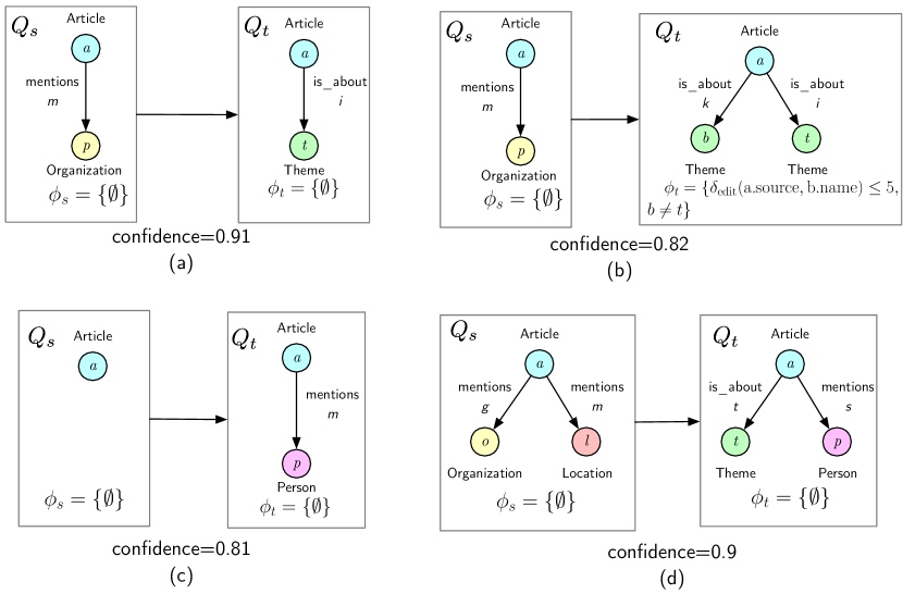
Figure 11. Example of GGDs discovered from GDelt with confidence $\geq 0.8$

7. Conclusion and Future Work

We have introduce GGDMiner, a framework designed to discover Graph Generating Dependencies (GGDs) for the purpose of graph data profiling. GGDMiner is able to identify interesting graph patterns and attribute similarities that succinctly describe a dataset. We employ the Answer Graph, which is a compact representation of the graph pattern matches, throughout the GGDMiner processes. This allows us to confirm which candidate pairs qualify as a GGD without the need for decompression (defactorization).

Our results also show that even with a small number of edges, GGDMiner can discover GGDs that can cover from 70% to 97% of the graph. We demonstrated that the discovered GGDs can also be used to understand and ensure the quality of the graph data. Each one of the methods used in each of the steps in GGDMiner can be treated as a separate problem. Our goal in this paper is to provide a framework-like solution for the discovery of GGDs with a common representation (Answer Graph) which can be used as a baseline for future contributions in the area and also can be easily extended to use different methods in each specific part of the framework. In future work, we plan to further investigate the choice of parameters of GGDMiner according to the dataset, extend GGDMiner to support other methods in the framework, support the discovery of other types of graph data dependencies that can use the same steps, and parallelize its execution to further improve scalability.

- (1)
- Abedjan et al. (2018) Ziawasch Abedjan, Lukasz Golab, Felix Naumann, and Thorsten Papenbrock. 2018. Data Profiling. Morgan & Claypool Publishers. https://doi.org/10.2200/S00878ED1V01Y201810DTM052
- Abul-Basher et al. (2021) Zahid Abul-Basher, Nikolay Yakovets, Parke Godfrey, Stanley Clark, and Mark H. Chignell. 2021. Answer Graph: Factorization Matters in Large Graphs. In Proceedings of the 24th International Conference on Extending Database Technology, EDBT 2021, Nicosia, Cyprus, March 23 - 26, 2021, Yannis Velegrakis, Demetris Zeinalipour-Yazti, Panos K. Chrysanthis, and Francesco Guerra (Eds.). OpenProceedings.org, 493–498. https://doi.org/10.5441/002/edbt.2021.57
- Alipourlangouri and Chiang (2022) Morteza Alipourlangouri and Fei Chiang. 2022. Discovery of Keys for Graphs [Extended Version]. https://doi.org/10.48550/ARXIV.2205.15547
- Angles et al. (2020) Renzo Angles, János Benjamin Antal, Alex Averbuch, Peter A. Boncz, Orri Erling, Andrey Gubichev, Vlad Haprian, Moritz Kaufmann, Josep-Lluís Larriba-Pey, Norbert Martínez-Bazan, József Marton, Marcus Paradies, Minh-Duc Pham, Arnau Prat-Pérez, Mirko Spasic, Benjamin A. Steer, Gábor Szárnyas, and Jack Waudby. 2020. The LDBC Social Network Benchmark. CoRR abs/2001.02299 (2020). arXiv:2001.02299 http://arxiv.org/abs/2001.02299
- Bonifati et al. (2018) Angela Bonifati, George H. L. Fletcher, Hannes Voigt, and Nikolay Yakovets. 2018. Querying Graphs. Morgan & Claypool Publishers. https://doi.org/10.2200/S00873ED1V01Y201808DTM051
- Dong et al. (2011) Wei Dong, Charikar Moses, and Kai Li. 2011. Efficient K-Nearest Neighbor Graph Construction for Generic Similarity Measures. In Proceedings of the 20th International Conference on World Wide Web (Hyderabad, India) (WWW ’11). Association for Computing Machinery, New York, NY, USA, 577–586. https://doi.org/10.1145/1963405.1963487
- Dürsch et al. (2019) Falco Dürsch, Axel Stebner, Fabian Windheuser, Maxi Fischer, Tim Friedrich, Nils Strelow, Tobias Bleifuß, Hazar Harmouch, Lan Jiang, Thorsten Papenbrock, and Felix Naumann. 2019. Inclusion Dependency Discovery: An Experimental Evaluation of Thirteen Algorithms. In Proceedings of the 28th ACM International Conference on Information and Knowledge Management (Beijing, China) (CIKM ’19). Association for Computing Machinery, New York, NY, USA, 219–228. https://doi.org/10.1145/3357384.3357916
- Elseidy et al. (2014) Mohammed Elseidy, Ehab Abdelhamid, Spiros Skiadopoulos, and Panos Kalnis. 2014. GraMi: Frequent Subgraph and Pattern Mining in a Single Large Graph. Proc. VLDB Endow. 7, 7 (mar 2014), 517–528. https://doi.org/10.14778/2732286.2732289
- Fan et al. (2022) Wenfei Fan, Wenzhi Fu, Ruochun Jin, Ping Lu, and Chao Tian. 2022. Discovering Association Rules from Big Graphs. Proc. VLDB Endow. 15, 7 (jun 2022), 1479–1492. https://doi.org/10.14778/3523210.3523224
- Fan et al. (2011) Wenfei Fan, Floris Geerts, Jianzhong Li, and Ming Xiong. 2011. Discovering Conditional Functional Dependencies. IEEE Transactions on Knowledge and Data Engineering 23, 5 (2011), 683–698. https://doi.org/10.1109/TKDE.2010.154
- Fan et al. (2020) Wenfei Fan, Chunming Hu, Xueli Liu, and Ping Lu. 2020. Discovering Graph Functional Dependencies. ACM Trans. Database Syst. 45, 3, Article 15 (sep 2020), 42 pages. https://doi.org/10.1145/3397198
- Fan and Lu (2019) Wenfei Fan and Ping Lu. 2019. Dependencies for Graphs. ACM Trans. Database Syst. 44, 2, Article 5 (feb 2019), 40 pages. https://doi.org/10.1145/3287285
- Fan et al. (2015) Wenfei Fan, Xin Wang, Yinghui Wu, and Jingbo Xu. 2015. Association Rules with Graph Patterns. Proc. VLDB Endow. 8, 12 (aug 2015), 1502–1513. https://doi.org/10.14778/2824032.2824048
- Galárraga et al. (2015) Luis Galárraga, Christina Teflioudi, Katja Hose, and Fabian M. Suchanek. 2015. Fast rule mining in ontological knowledge bases with AMIE+. VLDB J. 24, 6 (2015), 707–730. https://doi.org/10.1007/S00778-015-0394-1
- Galárraga et al. (2013) Luis Antonio Galárraga, Christina Teflioudi, Katja Hose, and Fabian Suchanek. 2013. AMIE: Association Rule Mining under Incomplete Evidence in Ontological Knowledge Bases. In Proceedings of the 22nd International Conference on World Wide Web (Rio de Janeiro, Brazil) (WWW ’13). Association for Computing Machinery, New York, NY, USA, 413–422. https://doi.org/10.1145/2488388.2488425
- Jiang et al. (2013) Chuntao Jiang, Frans Coenen, and Michele Zito. 2013. A survey of frequent subgraph mining algorithms. The Knowledge Engineering Review 28, 1 (2013), 75–105. https://doi.org/10.1017/S0269888912000331
- Jiang et al. (2014) Yu Jiang, Guoliang Li, Jianhua Feng, and Wen-Syan Li. 2014. String Similarity Joins: An Experimental Evaluation. Proc. VLDB Endow. 7, 8 (apr 2014), 625–636. https://doi.org/10.14778/2732296.2732299
- Kruse and Naumann (2018) Sebastian Kruse and Felix Naumann. 2018. Efficient Discovery of Approximate Dependencies. Proc. VLDB Endow. 11, 7 (mar 2018), 759–772. https://doi.org/10.14778/3192965.3192968
- Kwashie et al. (2015) Selasi Kwashie, Jixue Liu, Jiuyong Li, and Feiyue Ye. 2015. Efficient Discovery of Differential Dependencies Through Association Rules Mining. In Databases Theory and Applications, Mohamed A. Sharaf, Muhammad Aamir Cheema, and Jianzhong Qi (Eds.). Springer International Publishing, Cham, 3–15.
- Kwashie et al. (2019) Selasi Kwashie, Lin Liu, Jixue Liu, Markus Stumptner, Jiuyong Li, and Lujing Yang. 2019. Certus: An Effective Entity Resolution Approach with Graph Differential Dependencies (GDDs). Proc. VLDB Endow. 12, 6 (feb 2019), 653–666. https://doi.org/10.14778/3311880.3311883
- Li et al. (2011) Guoliang Li, Dong Deng, Jiannan Wang, and Jianhua Feng. 2011. Pass-Join: A Partition-Based Method for Similarity Joins. Proc. VLDB Endow. 5, 3 (nov 2011), 253–264. https://doi.org/10.14778/2078331.2078340
- Liu et al. (2012) Jixue Liu, Jiuyong Li, Chengfei Liu, and Yongfeng Chen. 2012. Discover Dependencies from Data—A Review. IEEE Transactions on Knowledge and Data Engineering 24, 2 (2012), 251–264. https://doi.org/10.1109/TKDE.2010.197
- Moussaoui et al. (2016) Mohamed Moussaoui, Montaceur Zaghdoud, and Jalel Akaichi. 2016. POSGRAMI: Possibilistic Frequent Subgraph Mining in a Single Large Graph. In Information Processing and Management of Uncertainty in Knowledge-Based Systems, Joao Paulo Carvalho, Marie-Jeanne Lesot, Uzay Kaymak, Susana Vieira, Bernadette Bouchon-Meunier, and Ronald R. Yager (Eds.). Springer International Publishing, Cham, 549–561.
- Nguyen et al. (2021) Lam B. Q. Nguyen, Loan T. T. Nguyen, Ivan Zelinka, Vaclav Snasel, Hung Son Nguyen, and Bay Vo. 2021. A Method for Closed Frequent Subgraph Mining in a Single Large Graph. IEEE Access 9 (2021), 165719–165733. https://doi.org/10.1109/ACCESS.2021.3133666
- Papenbrock et al. (2015) Thorsten Papenbrock, Jens Ehrlich, Jannik Marten, Tommy Neubert, Jan-Peer Rudolph, Martin Schönberg, Jakob Zwiener, and Felix Naumann. 2015. Functional dependency discovery: An experimental evaluation of seven algorithms. Proceedings of the VLDB Endowment 8, 10 (2015), 1082–1093.
- Pena et al. (2019) Eduardo H. M. Pena, Eduardo C. de Almeida, and Felix Naumann. 2019. Discovery of Approximate (and Exact) Denial Constraints. Proc. VLDB Endow. 13, 3 (nov 2019), 266–278. https://doi.org/10.14778/3368289.3368293
- Schirmer et al. (2020) Philipp Schirmer, Thorsten Papenbrock, Ioannis Koumarelas, and Felix Naumann. 2020. Efficient Discovery of Matching Dependencies. ACM Trans. Database Syst. 45, 3, Article 13 (aug 2020), 33 pages. https://doi.org/10.1145/3392778
- Shimomura et al. (2020) Larissa C. Shimomura, George Fletcher, and Nikolay Yakovets. 2020. GGDs: Graph Generating Dependencies. In Proceedings of the 29th ACM International Conference on Information & Knowledge Management (Virtual Event, Ireland) (CIKM ’20). Association for Computing Machinery, New York, NY, USA, 2217–2220. https://doi.org/10.1145/3340531.3412149
- Shimomura et al. (2022) Larissa C. Shimomura, Nikolay Yakovets, and George Fletcher. 2022. Reasoning on Property Graphs with Graph Generating Dependencies. arXiv:2211.00387 [cs.DB]
- Song and Chen (2011) Shaoxu Song and Lei Chen. 2011. Differential Dependencies: Reasoning and Discovery. ACM Trans. Database Syst. 36, 3, Article 16 (aug 2011), 41 pages. https://doi.org/10.1145/2000824.2000826
- Yan and Han (2002) Xifeng Yan and Jiawei Han. 2002. gSpan: graph-based substructure pattern mining. In 2002 IEEE International Conference on Data Mining, 2002. Proceedings. 721–724. https://doi.org/10.1109/ICDM.2002.1184038