The imprints of galaxy cluster internal dynamics on the Sunyaev-Zeldovich effect
Abstract
Context. Forthcoming measurements of the Sunyaev-Zeldovich (SZ) effect in galaxy clusters will dramatically improve our understanding of the main intra-cluster medium (ICM) properties and how they depend on the particular thermal and dynamical state of the associated clusters.
Aims. Using a sample of simulated galaxy clusters, whose dynamical history can be well known and described, we assess the impact of the ICM internal dynamics on both the thermal and kinetic SZ effects (tSZ and kSZ, respectively).
Methods. We produce synthetic maps of the SZ effect, both thermal and kinetic, for the simulated clusters obtained in a cosmological simulation produced by a cosmological Adaptive Mesh Refinement (AMR) code. For each galaxy cluster in the sample, its dynamical state is estimated by using a combination of well-established indicators. We use the correlations between SZ maps and cluster dynamical state, to look for the imprints of the evolutionary events, mainly mergers, on the SZ signals.
Results. While the tSZ effect only shows dependency on dynamical state in its radial distribution, the kinetic effect shows a remarkable correlation with this property: unrelaxed clusters present a higher radial profile and an overall stronger signal at all masses and radii. The reason for this correlation is the fuzziness of the ICM produced by recent merging episodes. Furthermore, the kSZ signal is correlated with rotation for relaxed clusters, while for the disturbed systems the effect is dominated by other motions such as bulk flows, turbulence, etc. The kSZ effect shows a dipolar pattern when averaging over cluster dynamical classes, especially for the relaxed population. This feature can be exploited to stack multiple kSZ maps in order to recover a stronger dipole signal that would be correlated with the global rotation properties of the sample.
Conclusions. The SZ effect can be used as a tool to estimate the dynamical state of galaxy clusters, especially to segregate those clusters with a quiescent evolution from those with a rich record of recent merger events. Our results suggest that the forthcoming observational data measuring the SZ signal in clusters could be used as a complementary strategy to classify the evolutionary history of galaxy clusters.
Key Words.:
cosmic background radiation – large-scale structure of Universe – Galaxies: clusters: intra-cluster medium – methods: numerical1 Introduction
Galaxy clusters (GCs) are collections of 50 to a few thousand galaxies held together by gravitational forces. These clusters have typical masses around and radius of . The majority of the mass in GCs, up to 84-90%, is in the form of dark matter (DM), while only 10-16% is in the form of baryonic matter, primarily hot gas known as the intra-cluster medium (ICM). Only 1-5% of the mass is composed of stars (Cimatti et al. 2019).
The ICM is an almost fully ionised plasma at temperatures around . This plasma extends throughout the entire cluster volume and emits X-rays predominantly through thermal bremsstrahlung (Sarazin 1988; Birkinshaw 1999). Electrons in the ICM are not only scattered by ions (bremsstrahlung), but can themselves scatter photons. Hence, apart from being extremely luminous X-ray sources, GCs also leave an imprint on the cosmic microwave background (CMB; Penzias & Wilson 1979) through the Sunyaev-Zeldovich effect (SZ; Zeldovich & Sunyaev 1969), arising from the scattering of CMB photons off ICM electrons through the inverse Compton effect (see Rephaeli 1995; Birkinshaw 1999; Carlstrom et al. 2002; Mroczkowski et al. 2019, for reviews).
The SZ effect can be separated in two main components, the thermal (tSZ) and the kinetic (kSZ) effects. The thermal signal is produced as CMB photons travel through the ICM of a GC and get scattered, in any direction, by the random thermal motions of the ICM electrons and, since the ICM is very hot, it shifts the CMB spectrum towards higher frequencies. The change in the black-body CMB temperature () due to the tSZ effect (first calculated by Zeldovich & Sunyaev 1969 using the Kompaneets 1957 equation) is given by Mroczkowski et al. (2019):
| (1) |
where is the electron number density, the electron gas temperature, the electron mass, the Thomson scattering cross-section, the Boltzmann constant, and the speed of light. On the other hand, is a function of frequency and CMB temperature111The expression for can be the original, non-relativistic, diffusive solution provided by Zeldovich & Sunyaev (1969) or the one including the more complicated relativistic corrections by Rephaeli (1995)., is the so called Compton -parameter, that encapsulates the GC temperature and density distributions and is the physical distance travelled by the photon along the line-of-sight. We remark that considering the electron gas as an ideal gas (which due to the temperature and density regime is accurate enough), the equation of state is and, therefore, measures the electron pressure () integrated along the line-of-sight.
On the other hand, the kinetic effect arises from the fact that, due to the bulk motion of the GC and the internal movements of the ICM (rotation, turbulence, etc.), the scattering medium is moving with respect to the CMB reference frame (Hubble flow). The change in the CMB temperature due to the kSZ effect alone is given by (Sunyaev & Zeldovich 1980; Mroczkowski et al. 2019):
| (2) |
where is the velocity along the line-of-sight and is the Compton -parameter for the kSZ effect. The sign criteria is such that if the gas is moving away from the observer (), it decreases the CMB temperature. In this case, encapsulates the kinematic structure of the cluster and its peculiar motion. Contrarily to the tSZ signal, the kinetic effect does not depend on frequency and, therefore, it cannot modify the CMB black-body spectrum. In this sense, the kSZ effect can be understood as a Doppler boost of CMB photons (e.g. Baxter et al. 2019). In fact, as Rephaeli (1995) pointed out, Eq. (2) can be obtained from a simple relativistic transformation.
The kSZ signal can be further split in different contributions. The one that contributes the most is the bulk or monopole component (e.g. Hand et al. 2012; Chen et al. 2022), which is due to the movement of the cluster as a whole with respect to the CMB. Nevertheless, if we subtract this component, we get more contributions due to the ICM internal motions such as rotation, which produces a dipole-like signal (e.g. Cooray & Chen 2002; Chluba & Mannheim 2002), or random motions due to turbulence which fill most of the ICM volume (e.g. see Vazza et al. 2017; Vallés-Pérez et al. 2021a, b). While the monopole can be used to measure GC peculiar velocities, the other contributions are useful to understand the internal dynamics of the gas in GCs. The kinetic SZ signal remaining from the subtraction of the monopole has been studied especially for an ideal rotation alignment, that is, when the angular momentum is perpendicular to the line-of-sight. In this particular case, the dipole signal due to rotation maximises and the effect is known as the rotational kSZ signal (rkSZ; Cooray & Chen 2002; Chluba & Mannheim 2002). However, in general, the rotation axes will be randomly aligned, and hence, the dipole signal due to rotation will not necessarily be the dominant contribution after the monopole. Other ICM internal movements, such as turbulence or outflows, could contribute significantly.
Whereas the frequency-dependent tSZ effect is the dominant component and is relatively easy to observe, the kSZ effect, which generates a fainter frequency-independent signal, can be easily confused with primary CMB anisotropies (e.g. Colafrancesco 2007). Nevertheless, on small angular scales, where these anisotropies have minimal influence, the kSZ effect enables the measurement of gas peculiar velocities, particularly velocity gradients within the ICM (see Dupke & Bregman 2002 for a discussion on these measurements). Hence, in combination with X-ray emission and the tSZ signal, the kSZ effect can help disentangling the complex ICM velocity structure produced by AGN feedback, cosmological structure formation or turbulent motions (see, e.g. Battaglia et al. 2017; Simionescu et al. 2019). Moreover, since the kSZ signal is temperature independent and linearly proportional to electron density, it is especially convenient to explore low density and temperature regions such as the outskirts of galaxy clusters and groups of galaxies, thus having the potential of shedding light on the missing baryon problem (e.g. see Hernández-Monteagudo et al. 2015 for observational evidence or Planelles et al. 2018 for a computational approach). From a different point of view, the SZ effect measurements can be used to disentangle the nature of other components of the Universe such as dark matter or dark energy, as well as a tool to test the feasibility of different cosmological models (e.g. non-flat Universe) or other gravity theories (see, e.g. Alfano et al. 2023).
Currently, thanks to measurements carried out by observational facilities such as Planck (Ade et al. 2014), South Pole Telescope (SPT; Reichardt et al. 2013), Atacama Cosmology Telescope (ACT; Hasselfield et al. 2013) or Combined Array for Research in Millimeter-wave Astronomy (CARMA ; Plagge et al. 2013), the number of clusters studied using the SZ signal has increased significantly. Moreover, in the upcoming decades future X-ray missions, such as Xrism222https://xrism.isas.jaxa.jp/en/ and Athena333https://www.the-athena-x-ray-observatory.eu/en, are expected to provide high precision measurements of ICM motions. In a similar way, future mm/sub-mm facilities (see, for instance, AtLAST444https://www.atlast.uio.no/ or SKA555https://www.skao.int/) are expected to have enough resolution to be able to measure the ICM velocity field by means of the kSZ effect. This synergy between future X-ray and mm/sub-mm observations will provide us unprecedented insight on the ICM thermodynamic properties.
Many successful attempts to measure bulk motions with the kSZ effect have been carried out so far (e.g. Hand et al. 2012; Soergel et al. 2016; Hill et al. 2016; Chen et al. 2022). Concerning the internal movements contribution to the kSZ effect, an early attempt to produce a spatially resolved map of the kSZ signal in a galaxy cluster was presented by Sayers et al. (2013). An improved measurement was provided by Adam et al. (2017), who detected a dipolar structure in the kSZ signal of the merging cluster MACS J0717.5+3745. The signal was consistent with two sub-clusters, moving with velocities of several thousand , one moving away and the other approaching the observer. In Matilla & Haiman (2020), the authors study the viability of statistically detecting a rotational kSZ signal through the combination of CMB data across numerous galaxies, where the spin orientation can be spectroscopically estimated.
Other recent observational efforts to further study gas thermodynamics with both thermal and kinetic SZ are Schaan et al. (2016, 2021), where the authors use both effects to study the baryon density and pressure profiles of galactic haloes, finding that they are shallower than their DM counterparts. In a similar direction, Amodeo et al. (2021) constrain the amount of non-thermal pressure inside the virial radius of GCs and Mallaby-Kay et al. (2023) present a novel hybrid estimator to measure kSZ, putting constraints on the thermodynamic properties of galaxy haloes. Furthermore, regarding the cluster dynamical state and SZ connection, Adam et al. (2023) confirm that the observed disturbed clusters have less concentrated and shallower electron pressure profiles compared to what would be expected for a relaxed cluster.
Early works using numerical simulations, such as Springel et al. (2001), already put constraints on the mean Comptonization due to tSZ. More recent works (e.g. Planelles et al. 2017, 2018; Lokken et al. 2023) have further expanded our knowledge studying the tSZ effect on clusters and their surroundings producing mock maps and scaling relations. Moreover, other studies such as Baldi et al. (2018) or Altamura et al. (2023) have focused on the kSZ effect, trying to disentangle the different components (namely the cluster peculiar velocity and rotation) producing the signal.
In view of the upcoming observational efforts, and as a continuation of the computational studies aforementioned, in this paper we aim to study the tSZ and kSZ effects on a sample of simulated galaxy clusters () at different redshifts and dynamical states to provide results to interpret and lead future observations. For each simulated cluster in our sample we produce maps of the tSZ and kSZ signals. With these results, we study the mean features of both SZ effects, and look for possible correlations with the dynamical state of the clusters in our sample. We present the individual results for several prototypical clusters, together with a statistical approach considering the whole sample. The redshift evolution is also considered.
The structure of the manuscript is a follows. In Sect. 2, we give the details of the simulation, the halo finder and the cluster sample, and we describe how the dynamical state of the clusters is defined. In Sect. 3, we describe the results obtained for the analysis of single clusters and the whole sample. Finally, we conclude and discuss our results in Sect. 4.
2 Methods
2.1 The simulation
In this work we examine a numerical simulation performed with the cosmological code MASCLET (Quilis 2004; Quilis et al. 2020). This code, designed primarily for cosmological purposes, employs (magneto-)hydrodynamics and -Body techniques. The gaseous (collisional) component is evolved using high-resolution shock-capturing methods, while the DM component is evolved using an -body multilevel Particle-Mesh (PM) scheme (Hockney & Eastwood 1988). The gravity solver ensures the coupled evolution of both components. Also, to enhance spatial and temporal resolution, MASCLET incorporates an adaptive mesh refinement (AMR) scheme.
The simulation encompasses a periodic, cubic domain with a size of , discretised into cubical cells. It assumes a flat CDM cosmology characterised by a matter density parameter (), a baryon density parameter , and a Hubble parameter . The initial conditions originate from a realisation of the primordial Gaussian random field, assuming a spectral index of and an amplitude resulting in . These conditions are set up at redshift using a CDM transfer function (Eisenstein & Hu 1998). The chosen cosmological parameter values are in line with the latest findings reported by Planck Collaboration et al. (2020).
Starting from the initial conditions and evolving them until the present time using a low-resolution run with equal-mass particles, we select regions that meet specific refinement criteria to establish three levels of refinement (, and ) within the AMR scheme. In these initially refined levels, the DM component is sampled with particles that are 8, 64, and 512 times lighter than those employed for regions in . As the evolution progresses, local baryonic and DM densities are utilised to create finer grids, ultimately reaching a maximum refinement level of . The ratio between cell sizes for a given level () and its parent level () is , striking a balance between the prevention of numerical instabilities and the increase in resolution. This enables us to achieve a peak physical resolution of approximately at . With four different DM particle species, the mass resolution amounts to approximately , equivalent to using particles in the entire computational domain.
In addition to gravity, the simulation takes into account cooling mechanisms (free-free, inverse Compton, atomic and molecular cooling for primordial gas) and heating mechanisms (UV background radiation; Haardt & Madau 1995).
2.2 Cluster sample and dynamical state
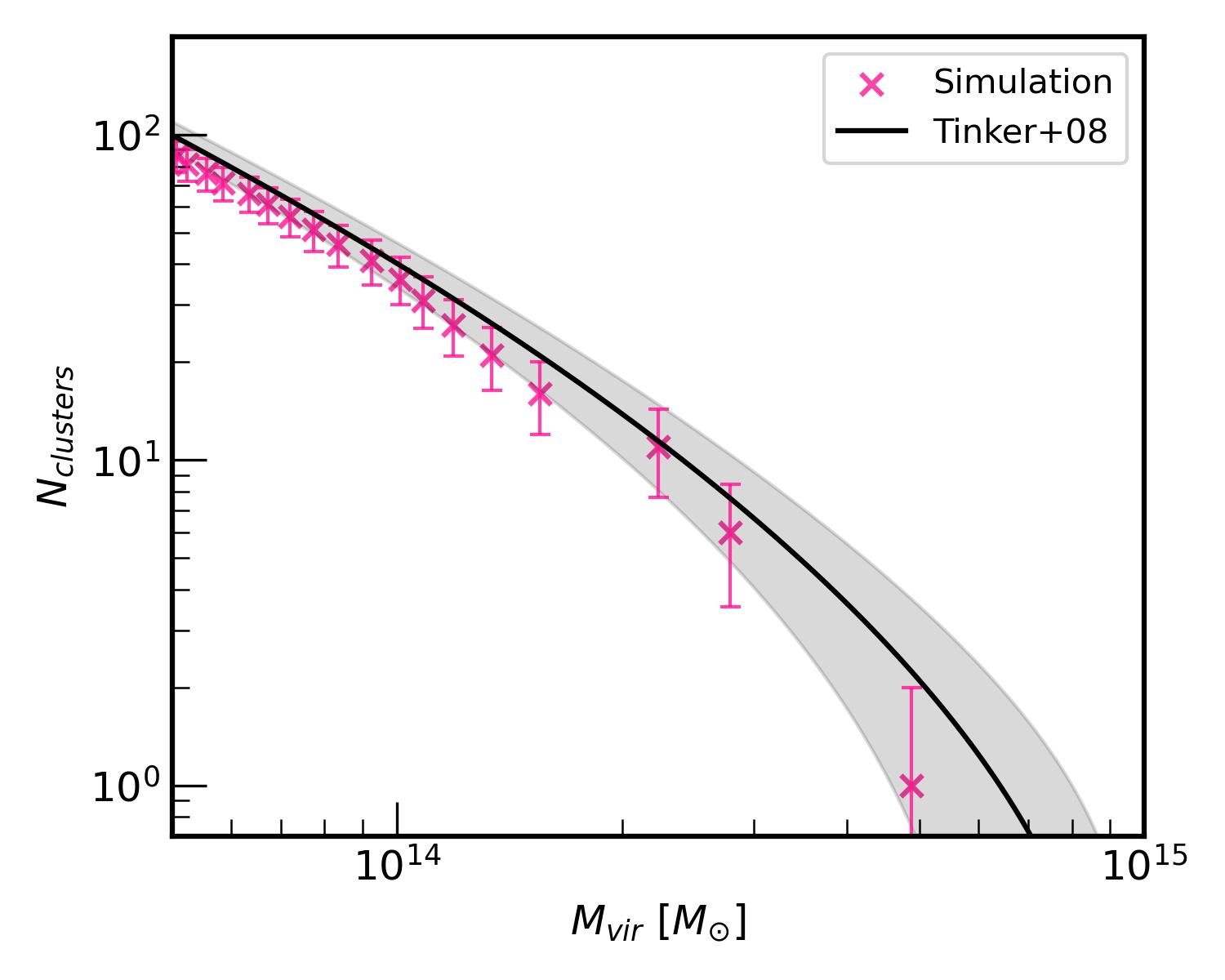
In order to identify the GCs produced in the simulation, we use the publicly available spherical overdensity halo finder ASOHF666https://github.com/dvallesp/ASOHF (see Planelles & Quilis 2010; Knebe et al. 2011; Vallés-Pérez et al. 2022, for more details). ASOHF finds DM bound structures (haloes) and substructures (subhaloes) in each snapshot of the simulation. In the simulation analysed in this work, ASOHF identifies haloes with virial mass777The virial mass, , is defined as the mass enclosed within a spherical region with radius equal to the virial radius, , which is defined as the radius of a sphere containing an average overdensity of . This critical overdensity for virialization, , depends on redshift (Bryan & Norman 1998). , , larger than at . In Figure 1, we plot the halo mass function of this simulation in the last iteration against the fit provided by Tinker et al. (2008). In the range fit and simulation are in a fair degree of agreement.
Since we want to study if and how the SZ effect changes depending on the dynamical state of the clusters, we need a robust estimation of this property. For this study, we employ the procedure described in Vallés-Pérez et al. (2023), in which a redshift-dependent combination of five different dynamical and morphological indicators is proposed to estimate the cluster dynamical state. While we refer the interested reader to the previous work, where a detailed description of the methodology employed to classify clusters according to their dynamical state is provided, here we briefly summarize the main procedure. We employ the following dynamical indicators of the DM halo:
-
•
Sparsity:
-
•
Ellipticity:
-
•
Centre offset:
-
•
Mean radial velocity:
-
•
Virial ratio:
where and are the masses enclosed within the radius with average overdensity and respectively, and are the smallest and largest semi-axes of the best fitting ellipsoid describing the DM mass distribution, and are the position of the density peak and centre of mass with respect to the simulation box centre, and are the mean radial velocity of DM particles and the circular velocity at , and , are the total kinetic and potential energy within the same aperture.
Each indicator, , has a redshift dependent threshold, , below which the cluster is classified as relaxed. Therefore, for a particular cluster, if every indicator satisfies the cluster is regarded as totally relaxed. Otherwise, the five dynamical indicators are combined to define a new parameter, , representing the degree of relaxedness of the considered halo (see Vallés-Pérez et al. 2023, for details on the definition of this parameter). Following this procedure, a given cluster which does not fall into the totally relaxed category will be classified as marginally relaxed if or unrelaxed whenever .
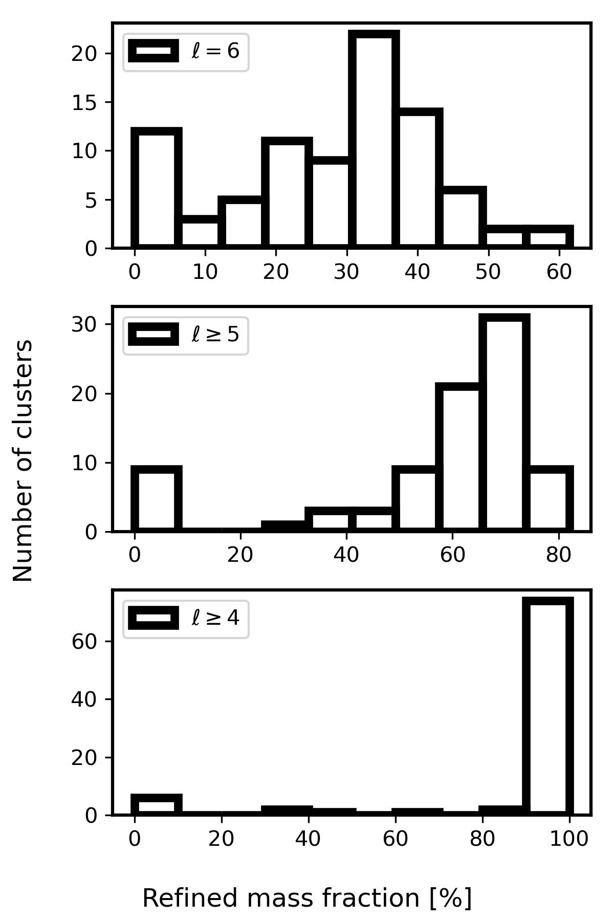
Applying this procedure to our cluster sample, we end up with , and clusters at . However, in order to avoid contamination of our results due to poorly resolved haloes, for every cluster in our sample we have quantified the fraction of the cluster mass inside that is refined at , and (see Fig. 2). According to these results, we have excluded from our sample all those haloes that fulfil that the mass fraction at each level, , is: , or . After pruning these poorly resolved haloes, we end up with a sample of , , and, hence, a total of clusters at , reducing our initial sample in a .
On the other hand, we are also interested in studying how the SZ effect in a particular cluster evolves with . For that purpose, we produce the merger tree from the ASOHF outputs and we trace the cluster population at backwards in cosmic time, so that we can analyse the evolution of each of those clusters individually.
2.3 SZ mock maps
There already exist packages to produce mock maps for the kinetic and thermal SZ effects, such as pyMSZ (Cui et al. 2018; Baldi et al. 2018). Nevertheless, they are made for particle data in SPH simulations and, hence, we would need to properly transform our AMR data in order to use them. For this reason, we have designed our own package in order to produce mock SZ observations from block-based AMR simulations888https://github.com/oscarmonllor99/MASC (in particular, for the MASCLET code).
The algorithm works as follows. For each cluster in our sample, we define a map of physical size centred on the DM density peak, with the maximum resolution of the simulation. In the current version of our algorithm, the map line-of-sight has to be parallel to one of the three coordinate axes of the computational domain. Once the map size is defined, we establish the integration width or depth, , within which we integrate Eqs. (1) and (2). In this case, we choose and we centre the integration in the density peak so that the integration interval is . Then, in order to calculate the -value in each pixel, we integrate, using the rectangle rule, the former equations along the photon path with an integration step equal to the maximum resolution of our AMR grid. The integration is done at fixed , that is, using just one snapshot for each case. This is because the photon crossing time, , is much smaller than the timescale for typical ICM motions, , which we define as the timescale on which the ICM could change noticeably its structure at the considered scales due to its internal dynamics (see Fig. 3 of Vallés-Pérez et al. 2021a). In this regard, since the gas moves at (e.g. Simionescu et al. 2019) and , we have . Thus, we should not expect the density, temperature and velocity fields to change significantly during the photon crossing time.
Since our simulation does not take into account stellar feedback nor AGN, overcooling affects to small volumes of the clusters, leading to unphysical values of density and temperature, and therefore, of parameters. To clear up this unwanted effect, we set up an upper comoving baryon density threshold for all cells involved in the integrated quantities along the line-of-sight. After some experimentation, we chose the value . Finally, since the Compton scattering is significantly produced only in the hot-ICM phase, we eliminate from our calculation those cells with . With both thresholds we assure that all the cells contributing to the calculation have typical ICM values. In practice, for all clusters, only of the volume is dismissed.
To overcome the contained size of our sample, and only to increase the statistics when needed, we have considered the projections along the , and axes, that is, projections on the , and planes, for each individual cluster as three different clusters in our extended sample. In this manner, the number of objects in the sample can be increased and get closer to the observational conditions in which no privileged direction is considered.
2.4 Mass normalization
In order to analyze the SZ signal dependence on the clusters’ dynamical state, we should get rid of implicit dependencies on other quantities like, for instance, mass. To do this, we need to find a mass dependence for each effect. For the thermal signal we have:
| (3) |
where we have used that is the mean surface density, the self-similar temperature-mass relation for the mean ICM temperature (e.g. Voit 2005, note that is a function of redshift that is not relevant, since the normalization is done at fixed ) and the fact that, by definition, . On the other hand, for the kinetic part we have:
| (4) |
where we consider that the average ICM velocity scales as the circular velocity at the virial radius and, hence, , being a function of redshift, which will not contribute to our normalization, since it is done at fixed .
Although based on simple arguments, the obtained scaling relations, Eqs. (3) and (4), allow us to purge the mass dependence. As it is shown in the results presented in the next section, the clusters in our sample fit well to these scaling relations within the errors, except for the kSZ signal of relaxed clusters, that, as discussed in Sect. 3.1.1, should not follow this mass dependence.
3 Results
In this section, we present the results obtained from the analysis of the mock SZ maps produced for every cluster in the sample. First, in Sect. 3.1, we focus on the results at , and later, in Sect. 3.2, we extent the analysis to the effect of cosmic evolution on SZ effects. Throughout this work, unless otherwise specified, we use the term kinetic SZ effect (kSZ) to refer to the effect produced when the monopole is subtracted, that is, the kinetic effect produced by the gas movements within the ICM in the cluster’s reference rest frame.
3.1 Analysis of the SZ effect at
Taking into account the dynamical state of the haloes in our sample, we analyse their associated SZ signals at by means of scaling relations (Sect. 3.1.1), radial profiles (Sect. 3.1.3) and projected maps (Sect. 3.1.4) of the most relevant quantities in order to find trends between different dynamical classes. We also try to disentangle the relevance of rotation on the kinetic effect (Sect. 3.1.1 and 3.1.4). Additionally, in Sect. 3.1.2 we discuss how varying the line-of-sight direction can affect the signal (the projection effect), depending on cluster dynamical state.
3.1.1 Scaling relations
| Thermal SZ | Kinetic SZ | |||
|---|---|---|---|---|
| Dynamical state | ||||
| Relaxed | ||||
| Unrelaxed | ||||
| All | ||||
A well-known scaling relation is the one between the tSZ -parameter (e.g. Planck Collaboration et al. 2013), integrated within some specific radius (for example, ), and the mass enclosed within that aperture. This relation has also been confirmed from a numerical point of view (e.g. Planelles et al. 2017). In our case, we use this relation as a test to validate our results.
One of the goals of the present paper is to look for similar correlations and scaling relations for the kSZ effect. However, the analysis of this effect requires some cautions to be taken. Given that the kSZ signal can have positive and negative values, mean values are not a well suited election for this analysis. So as to compare with tSZ, we define the root mean square (RMS) of the pixel values of the mock kSZ maps999Since the mean value of the kSZ signal tends to zero, the RMS is practically equal to the standard deviation and, hence, it has the physical meaning of quantifying how much the signal deviates from zero.. In this manner, the kSZ is described with a positive quantity and is directly comparable to the mean of the pixel values of the tSZ map. Hence, we will use the mean -parameter instead of the integrated quantity for the tSZ effect in order to be consistent101010Note that the integral and the mean of the -parameter inside some radius will differ just by the factor corresponding to the integration area..
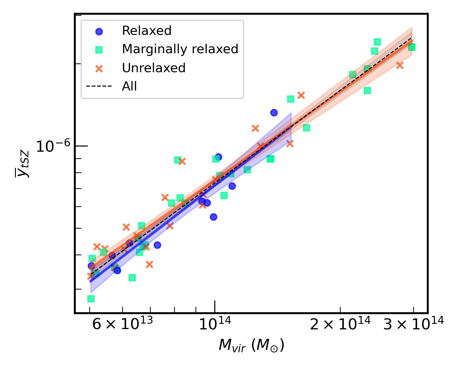
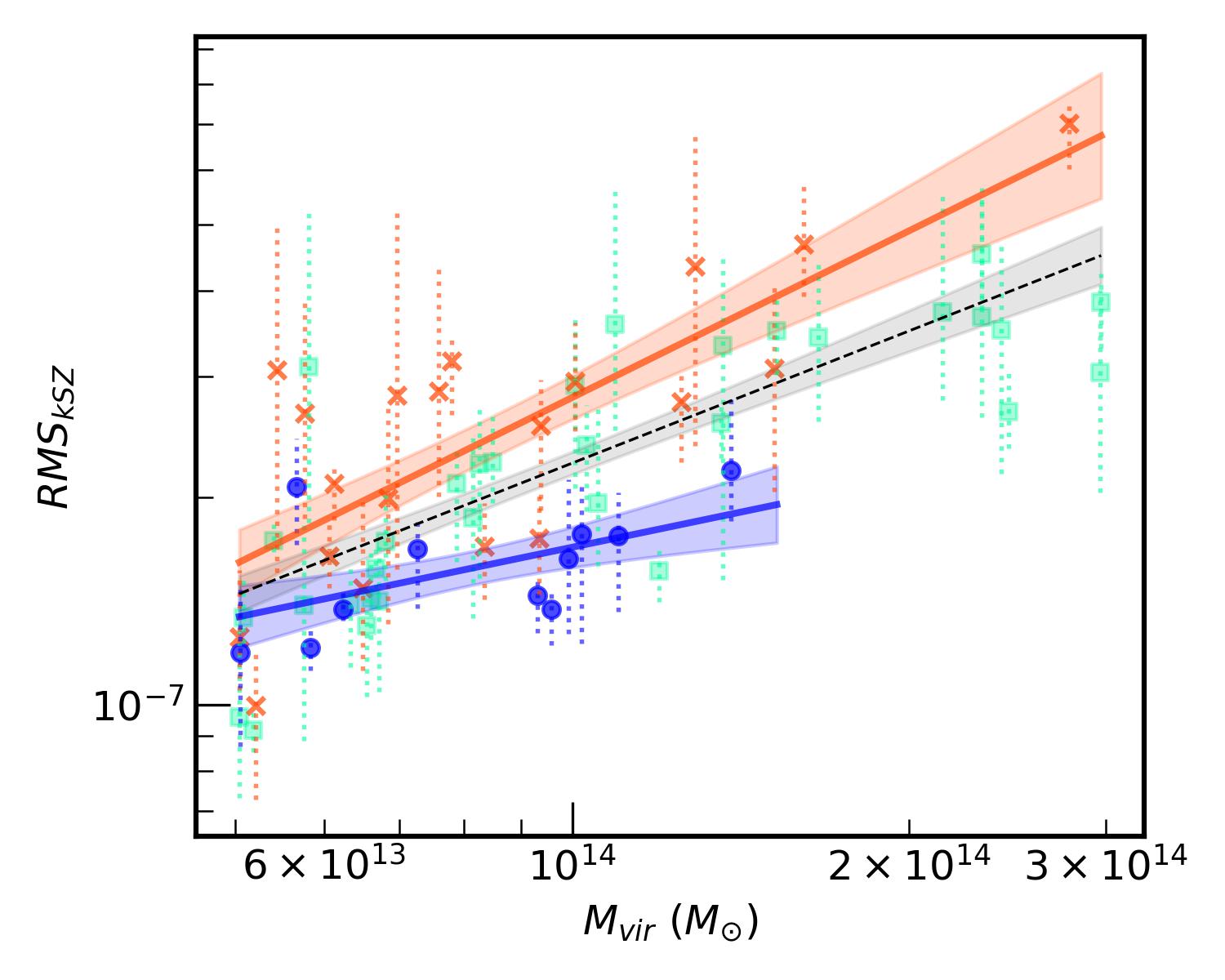
The results are presented in Fig. 3, where we show the scaling relation between and the mean (upper panel, denoted by ) and the RMS of the values (lower panel, denoted by ), both integrated in a aperture. The shown errobars correspond to the difference between the maximum and minimum values of and found in the three projections (, , ) of each cluster. Furthermore, in order to capture the difference between the trends of different cluster dynamical states, we perform a fit of the type where is the pivot mass. The best fitting parameters are presented in Table 1. No mass normalization is carried out here.
As expected, we obtain a tight correlation between and , without any significant difference due to dynamical state. The slopes are similar and consistent within the percentile errors shown, being also compatible with the theoretical in Eq. (3). Regarding the kSZ part, we observe more scatter, especially at lower mass, and we also obtain different trends depending on the cluster dynamical state, as shown by data fittings. The unrelaxed population shows a steeper () trend compared to the relaxed clusters (), but, more importantly, it shows a higher value at all masses compared to the relaxed population. As expected, the marginally relaxed population is halfway of the other two. Note how the fits for unrelaxed and all clusters are compatible, within their errors, with the theoretical value given in Eq. (4), while the relaxed fit is incompatible (within 1). Also note how the marginally relaxed population, which is the largest, follows almost perfectly the fit obtained for the whole sample (dashed line), which is the most consistent with the theoretical .
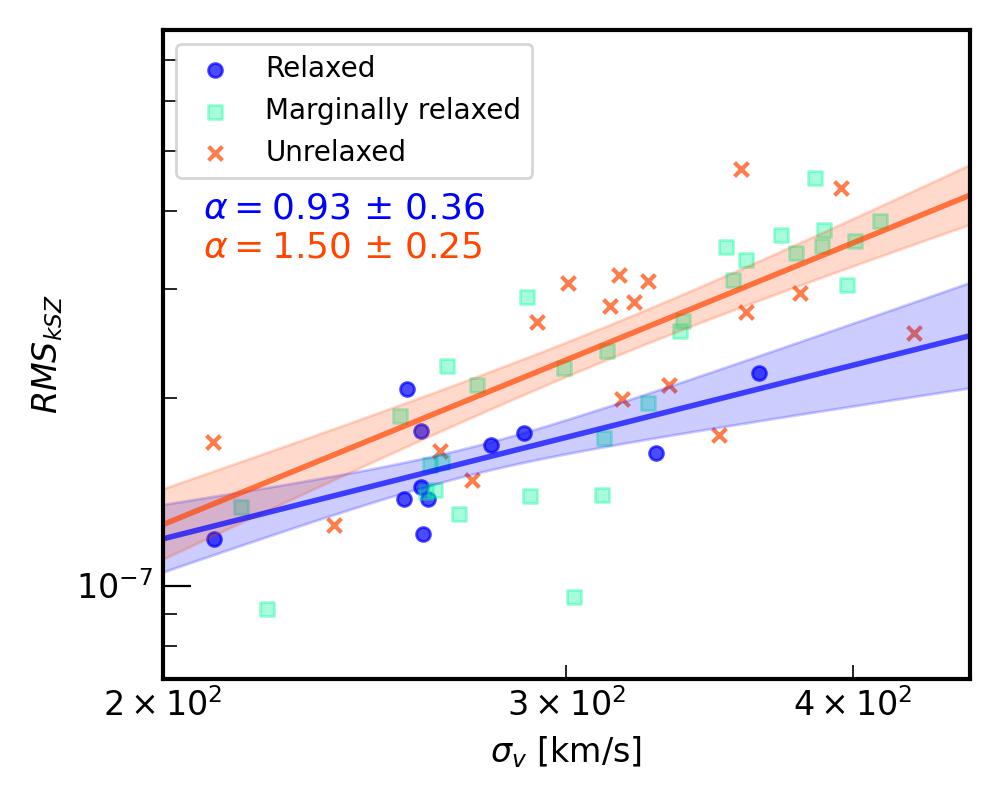
A plausible explanation for this separation in the kinetic effect, due to dynamical state, is the fact that the recent mergers and high accretion suffered by the unrelaxed clusters can trigger high velocity motions in the ICM (turbulence, outflows, etc.), and hence increase the overall kSZ signal of the cluster. In order to justify this fact, we show Fig. 4, where we plot the kSZ signal against the gas velocity dispersion with an analogous fit. The higher the velocity dispersion is, the more intense the kinetic effect gets. On the other hand, the unrelaxed population is shifted towards higher velocity dispersion, while the relaxed sample is shifted towards lower velocity dispersion, hence having the unrelaxed population, on average, an overall higher kSZ signal. Moreover, at fixed , the value of for disturbed clusters is higher than for the relaxed ones. More precisely, we obtain, approximately, and from the disturbed and relaxed fittings, respectively.
As mentioned above, the slope of the fit of the relaxed population for the is incompatible within 1 error with the theoretical value (). In order for a cluster of our sample to be relaxed, five different thresholds have to be fulfilled (see Sect. 2.2). This means that our criteria for considering a cluster as relaxed is quite restrictive and, hence, their dynamics need to be really calm. In fact, relaxed clusters are mostly supported by thermal pressure (they are close to be in hydrostatic equilibrium) and the kinetic pressure produced by ICM bulk motions does not play an important role in its support against gravitational collapse. Thus, it is possible to expect that the scaling derived for the kSZ mass dependence in Eq. (4) is overestimating the value of , which for our relaxed population is likely to be mostly contributed by residual motions, causing the disagreement. In principle, this difference in the slopes between relaxed and disturbed clusters for the kSZ signal could be used to infer the cluster dynamical state depending on which of both trends is followed.
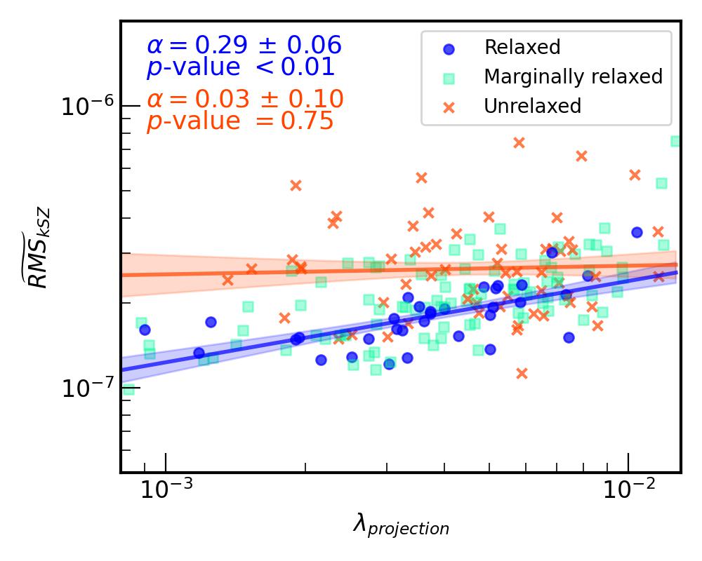
It is also interesting to study the connection between the kinetic effect and the cluster angular momentum. In order to mitigate the mass dependence for studying this correlation, we have to normalize the kinetic effect according to Eq. (4)111111We define as the RMS of the pixel values of the kinetic map normalized to . Equivalently, according to Eq. (3), we define . Besides, it would be desirable to study an angular momentum related quantity which is independent of mass. Thus, we have used the spin parameter presented in Bullock et al. (2001):
| (5) |
where is the magnitude of the total angular momentum inside a given radius , is the mass enclosed within that radius, and is the circular velocity at radius . Since we are working with projections, we will try to correlate to the kinetic signal only the component of the total angular momentum that lies in the projection plane. For instance, in the projection we will only consider , since the component of the rotation will not contribute to the kinetic signal, as it does not have velocity component along the line-of-sight.
The results are presented in Fig. 5, where we apply a similar fit to the data to disentangle the differences between populations. Note that, since we have three projections for each cluster, and the effect and angular momentum are different in each projection, we can treat each projection as an independent cluster signal, hence enhancing our statistics by a factor of three. Unrelaxed clusters hardly show any degree of correlation since the scatter is considerable and the fit is compatible with an horizontal line (, with -value ). On the other hand, for the relaxed case, we observe less scatter and a clear tendency to have a higher kSZ signal with increasing angular momentum (), which is translated into a small -value (that is, there exist correlation). Therefore, from this figure, we can infer that in the disturbed case, post-merger motions dominate over rotation and hence blur any possible correlation with angular momentum, while relaxed clusters are dominated by rotation, showing a clear correlation with .
3.1.2 Projection effects
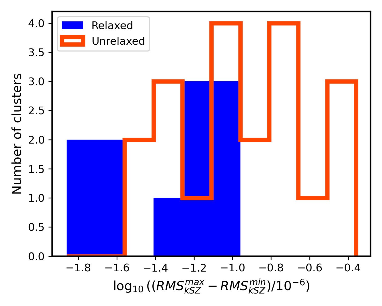
In Fig. 3, we show for each cluster the average value of the when considering three different lines-of-sight aligned with the Cartesian axes of the computational domain, whereas the error bars show the range between the maximum and minimum values over the three different projections. It is noticeable that the variation is in general significantly higher in disturbed clusters. In order to quantify this trend, in Fig. 6 we present an histogram of the variation of the RMS of the kSZ signal across the three different projections (lines-of-sight) for the relaxed and disturbed dynamical state classes. It is clear that low variations are dominated by relaxed clusters and large variations are mainly given in the unrelaxed cases. Hence, the impact of having the information projected in a certain plane is more important for disturbed clusters, since they tend to be aspherical and present significant substructure that can be erased due to projection effects. The opposite happens for relaxed clusters, as they generally have a rounder shape, minimizing the impact of projection.
For the tSZ signal, the projection effect is minimum compared to the kinetic part, to the point that the variation range is smaller than the data points in Fig. 3. A plausible explanation comes from the fact that the kSZ signal depends on , which has a different value depending on the projection, while the tSZ effect involves scalar quantities which do not vary with the direction of observation.
3.1.3 Radial profiles
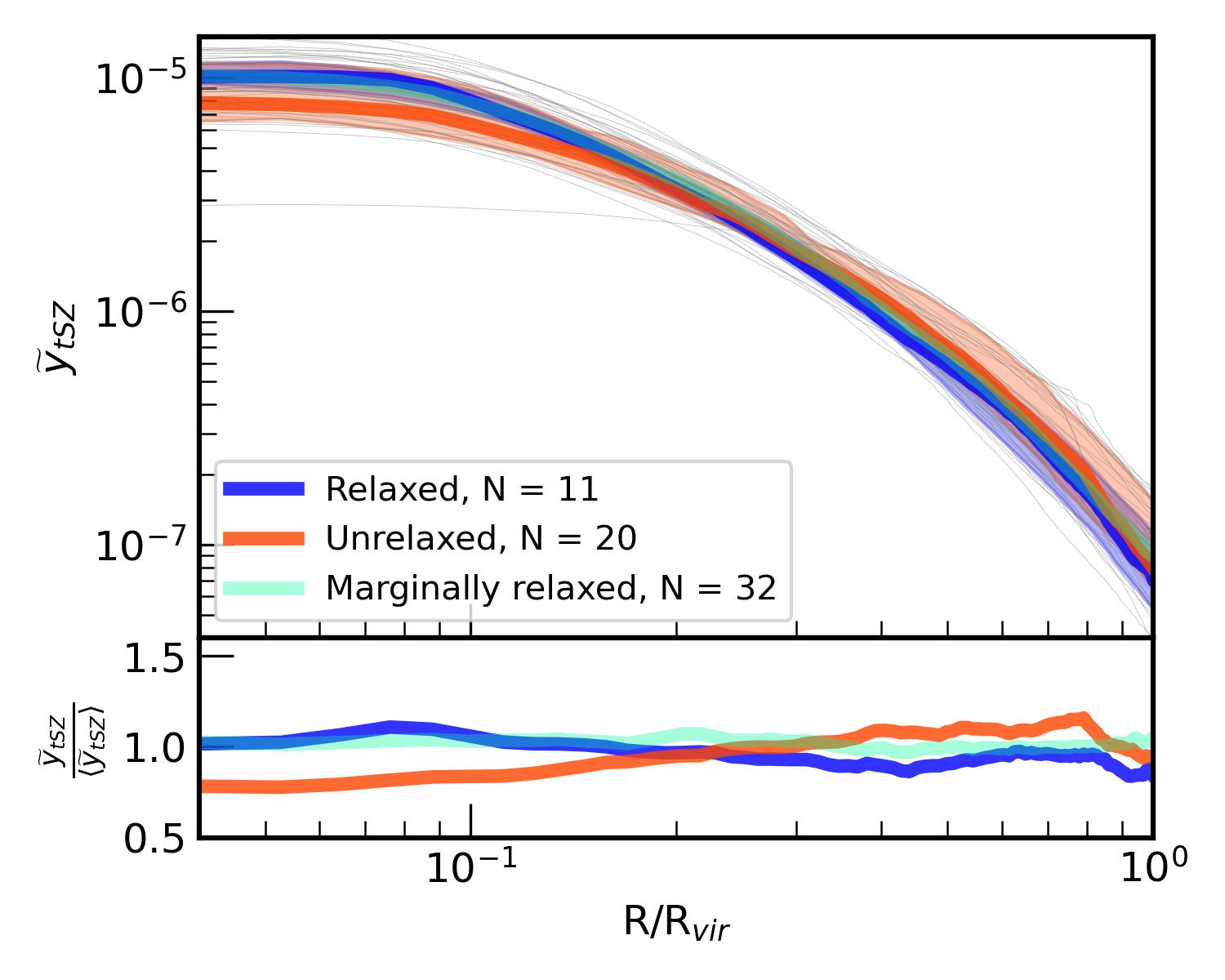
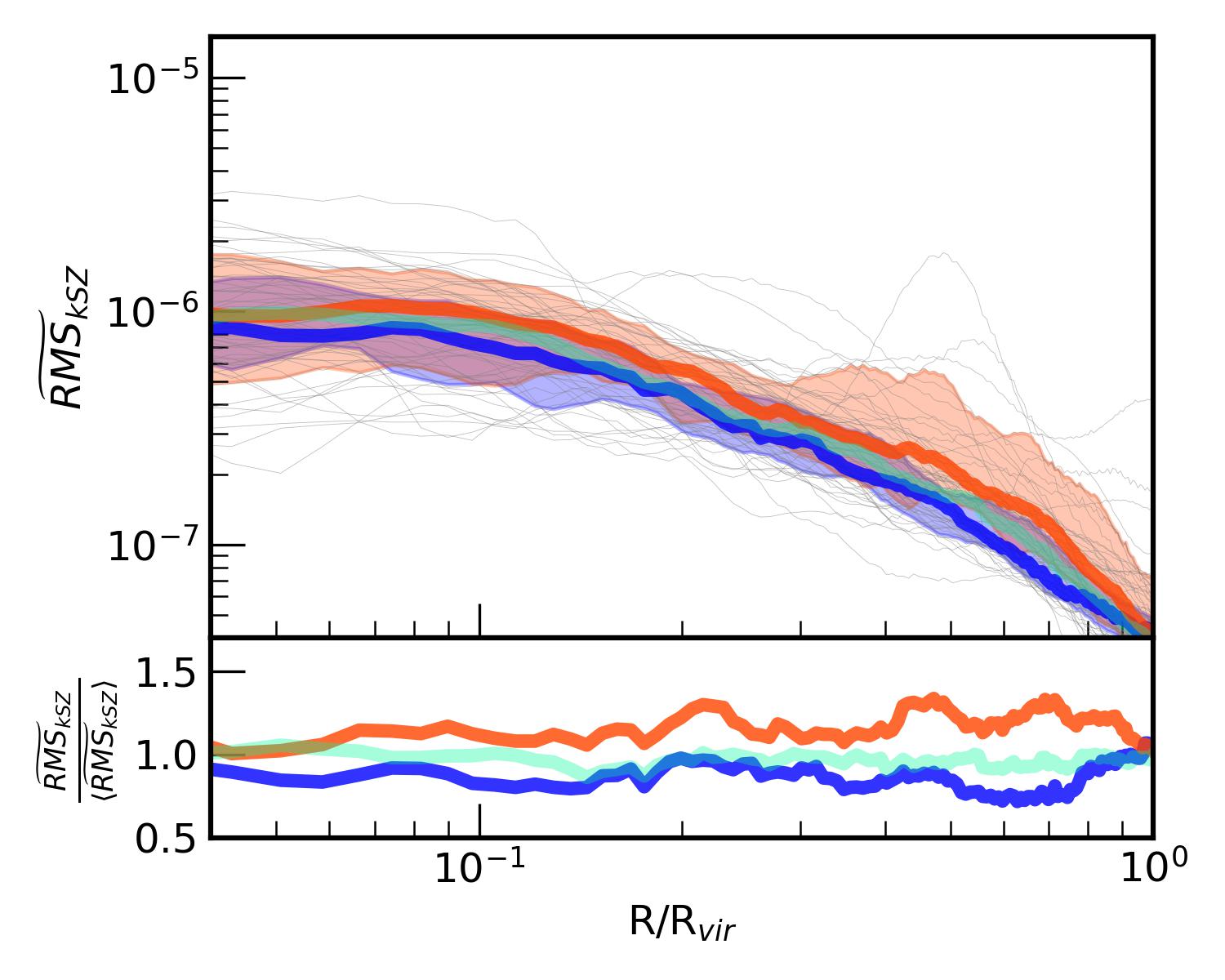
Another study to assess whether the cluster dynamical state affects the SZ signal would be to represent the radial profiles of this effect for each cluster population. In Fig. 7 we show the median profile at of the -parameter for the tSZ effect (top panel) and for the kSZ effect (bottom panel) for different cluster populations in terms of dynamical state. The thermal profile is obtained averaging over radial shells, whilst the kinetic profile is obtained computing its root mean square (RMS) in each shell. Since all clusters have been normalized to the same mass, , we employ the symbols and , respectively. This normalization ensures that the differences between populations are solely due to differences in the dynamical state. The shadowed regions represent the error corresponding to a 68% percentile. The small panels below show the same quantity divided by the mean across the three dynamical state populations, thus highlighting the differences between them.
For the tSZ effect we appreciate how the unrelaxed clusters have a flatter profile than the relaxed ones, which are more concentrated towards the cluster centre. Indeed, it can be seen that for the unrelaxed clusters show a greater signal, whereas for the relaxed clusters have a higher profile. This result is in agreement with recent observations carried out by Adam et al. (2023), where they confirm that disturbed clusters have a relatively flatter core and a shallow outer slope of the pressure profile (note that is an indirect measure of the electron gas pressure). On the other hand, for the kSZ effect we observe that the unrelaxed population has a higher value for all radii, being the shape of the profile equivalent in all dynamical states. Marginally relaxed clusters show a behaviour that is halfway of the other two. The explanation for the described facts is similar to the one given in Sect. 3.1.1: the thermal profile for unrelaxed clusters is less concentrated towards the centre due to, most importantly, recent merger(s), that move matter to the outer regions, hence rising there the SZ signal (both thermal and kinetic). Furthermore, turbulence and other motions caused by recent mergers suffered by the unrelaxed population produce high velocities that increase the overall kSZ signal, hence the overall higher profile for the unrelaxed population. Also, since marginally relaxed clusters are transitioning from unrelaxed to relaxed or vice versa, they show a middle term behaviour.
An important result given by theoretical studies (e.g. Rephaeli 1995) and observations (e.g. Adam et al. 2017) is the fact that the tSZ signal is approximately an order of magnitude larger than the kSZ signal, making the first one much easier to measure. This result is in agreement with the trend shown in Fig. 7, where the maximum values of the profiles satisfy that at the innermost region. Nevertheless, we see that in cluster outskirts, at , both effects become equally important, due to the higher importance of non-thermal motions in these regions.
3.1.4 Kinetic SZ maps and multipole expansion
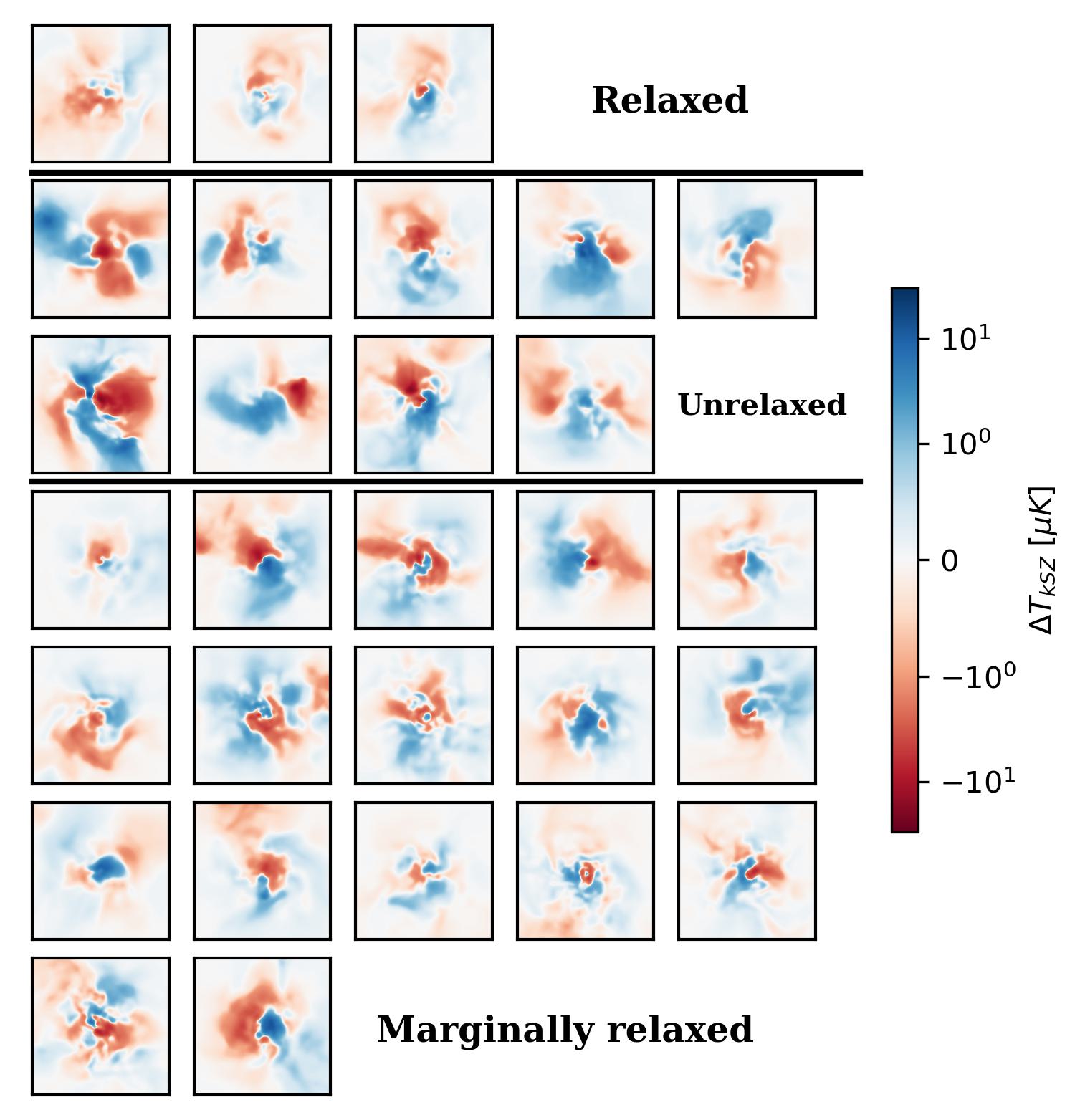
In Fig. 8 we present the kSZ map for all clusters in our sample with at , separated by dynamical state. The size of the maps is with the highest spatial resolution being and they are centred on the density peak. It can be easily seen that the major difference between relaxed and unrelaxed maps is the fact that the first have the signal significantly concentrated towards the inner regions whilst the second have more features and present a more extended signal across the cluster volume. This explains, for example, the radial profiles shown in Fig. 7, where the unrelaxed clusters clearly have a higher kSZ effect (and particularly towards the outer regions) or the scaling relation in Fig. 3 where the unrelaxed population show an overall higher kSZ signal for all masses.
On the other hand, because of cluster rotation, one should expect a dipole-like map once we have subtracted its bulk velocity and hence only internal motions remain (e.g. Baldi et al. 2018; Altamura et al. 2023). Nevertheless, this is only appreciated in some maps, since the orientation of the angular momentum does not necessarily rest in the plane of the map and, in some cases, it could be even perpendicular, hence leaving the kSZ signal only to ICM turbulence, other bulk flows, etc.
So as to quantify the importance of the rotation imprint in the kinetic SZ maps, we have performed a multipole expansion similar to that of Gouin et al. (2020), which is based on the methodology presented in Schneider & Bartelmann (1997). In these studies the multipole expansion is applied to matter surface density, while in our particular case it is applied to the kSZ map. The goal is to obtain general angular symmetries for each dynamical state class. In particular, we are interested in discerning the importance of the rotation on the maps, whose imprint is a dipole-like signal (e.g. Altamura et al. 2023). The multipole moments of a certain quantity () defined on a polar map () are given by:
| (6) |
where are the multipole moments and is the radial aperture over which we integrate. In our case, we have performed the integrals with , where the dominant part of the effect is produced (see Fig. 8).
The choice of the multipole expansion centre is crucial, as the centre of angular symmetries may not necessarily align with the image centre. Our choice for the new centre involves selecting the cell that corresponds to the arithmetic mean weighted by the absolute value of the signal. Through this straightforward recentring algorithm, we aim to minimise the introduction of a dipole signal in the expansion caused by the offset in the symmetry centre.
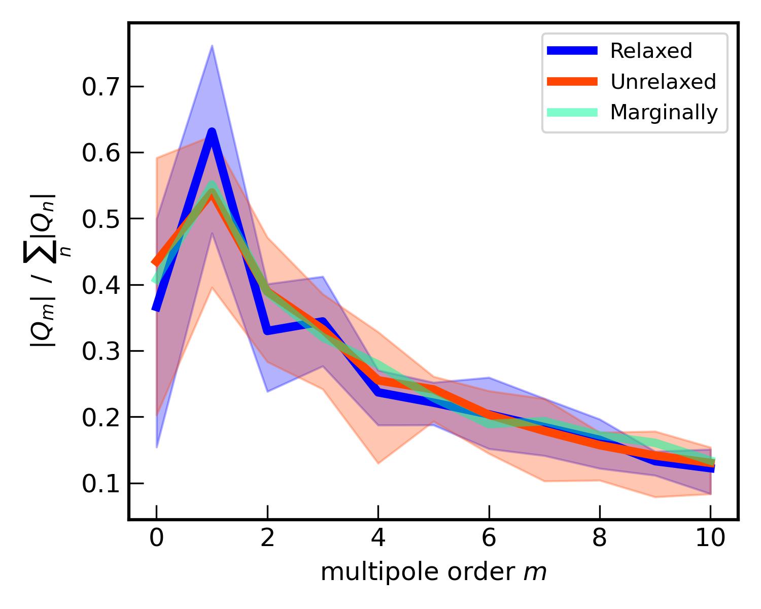
The results for the multipole expansion performed to all the sample kSZ maps are presented in Fig. 9, where we show the mean for each of the dynamical state classes of the module of the multipole expansion coefficients () normalised by the sum of the complete multipolar expansion. On average, the trends of the three populations are similar, being the dipole coefficient () clearly the most relevant, accounting for roughly of the sum over all coefficients. This implies that, in general, the dipole (and, in principle, rotation) is the most important contribution to the effect. Nevertheless, the shown 68% confidence intervals indicate that the weight of highly varies across all clusters, due to projection effects. Moreover, as it can be seen, the coefficients also contribute significantly to the signal and cannot be neglected. In fact, this is the main difference in the multipole expansion between disturbed and relaxed clusters: the first present a more prominent quadrupole behaviour and less dipole component. Considering the kSZ effect to be produced solely by rotation would result in a biased interpretation of the observations.
Fig. 9 shows an important feature of the kSZ signal that could be exploited by observations. Every kSZ map can show particular attributes but, when averaged over a significant number of clusters, the mean multipole expansion is dominated by the dipole and all the other coefficients become almost negligible, especially if only relaxed clusters are used. Hence, if properly recentred and oriented, many kSZ maps could be stacked and a dipole signal would emerge, which would be correlated to the global rotation properties of the sample. A similar procedure to the one described is applied in Xia et al. (2021) for intergalactic filaments.
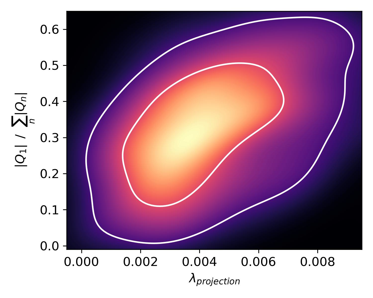
For a more in-depth exploration of the rotational influence on the kinetic signal, it is crucial to know the extent to which the dipole is attributable to rotation versus other contributing factors. In Fig. 10 we present a scaling relation for the whole sample between the module of the dipole coefficient () of the kinetic SZ map (normalised by the sum of all the multipole expansion coefficients) against the Bullock spin parameter () of the angular momentum for the three considered projections along the Cartesian axes. It can be seen that the dipole weight generally increases with increasing angular momentum in the corresponding projection. However, the scatter is considerable and, hence, apart from rotation, there are other ICM movements contributing to the dipole.
3.2 SZ signal evolution with redshift
In the present Section, we study how the kinetic and thermal SZ effects evolve with cosmic time, looking for a correlation between the SZ signal variations and the clusters’ dynamical state. First, we discuss the redshift evolution of the effect. Then, we analyse two particular cluster histories, in order to have a deeper description of this connection.
3.2.1 Redshift evolution
The SZ effect is essentially redshift independent (e.g. Carlstrom et al. 2002; Mroczkowski et al. 2019). Nevertheless, our clusters evolve with redshift due to the expansion of the Universe and, hence, this introduces an artificial redshift dependence that we have to take into account (e.g. see Schaan et al. 2021 for similar arguments). We define the haloes of our simulations according to the over-density , where is the matter density and is the background density, with being the critical density of the Universe. Thus, since is co-moving (independent of ), and , necessarily .
On the other hand, the physical size of the cluster is bigger at lower redshift due to the Universe expansion. If and are the physical and co-moving distance elements, respectively, then , where is the scale factor at a given . All in all, we have that the redshift evolution of the thermal effect is given by:
| (7) |
where is the co-moving line-of-sight distance and, thus, in the last step all the quantities inside the integral are comoving and, hence, redshift independent.
Similarly, the same procedure can be applied to the kinetic effect:
| (8) |
We want to emphasise that this redshift dependence is introduced in our calculations only because of the manner in which we define these objects. That is, the factor is only taking into account how our clusters are evolving with cosmic time (density and size) due to the expansion of the Universe. Nevertheless, the same object with the same physical size and physical density at and at arbitrary would produce the same effect at both redshifts, since there is no explicit dependence in Eq. (1).
Therefore, in order to analyse the redshift evolution of the effect due to dynamical state changes, we will remove the factor due to the intrinsic evolution of the cluster with the Universe expansion.
3.2.2 Individual cluster evolution
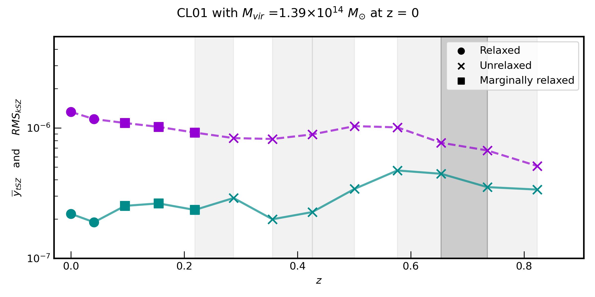
Although difficult to elucidate due to the complexity of the mass assembly histories of GCs (e.g. Vallés-Pérez et al. 2020), it is clear from the previous results that there is a connection between the cluster dynamical state and the SZ signal (especially the kinetic part). To make this even clearer, we have chosen two prototypical clusters from our population to analyse how their dynamical state and both tSZ and kSZ signals change with cosmic time, taking into account whether the clusters suffer minor or major mergers. The results are presented in Fig. 11, where we depict the cluster dynamical state, the kSZ (green) and tSZ (purple) signals and whether it has suffered a minor (major) merger in light (dark) grey bars.
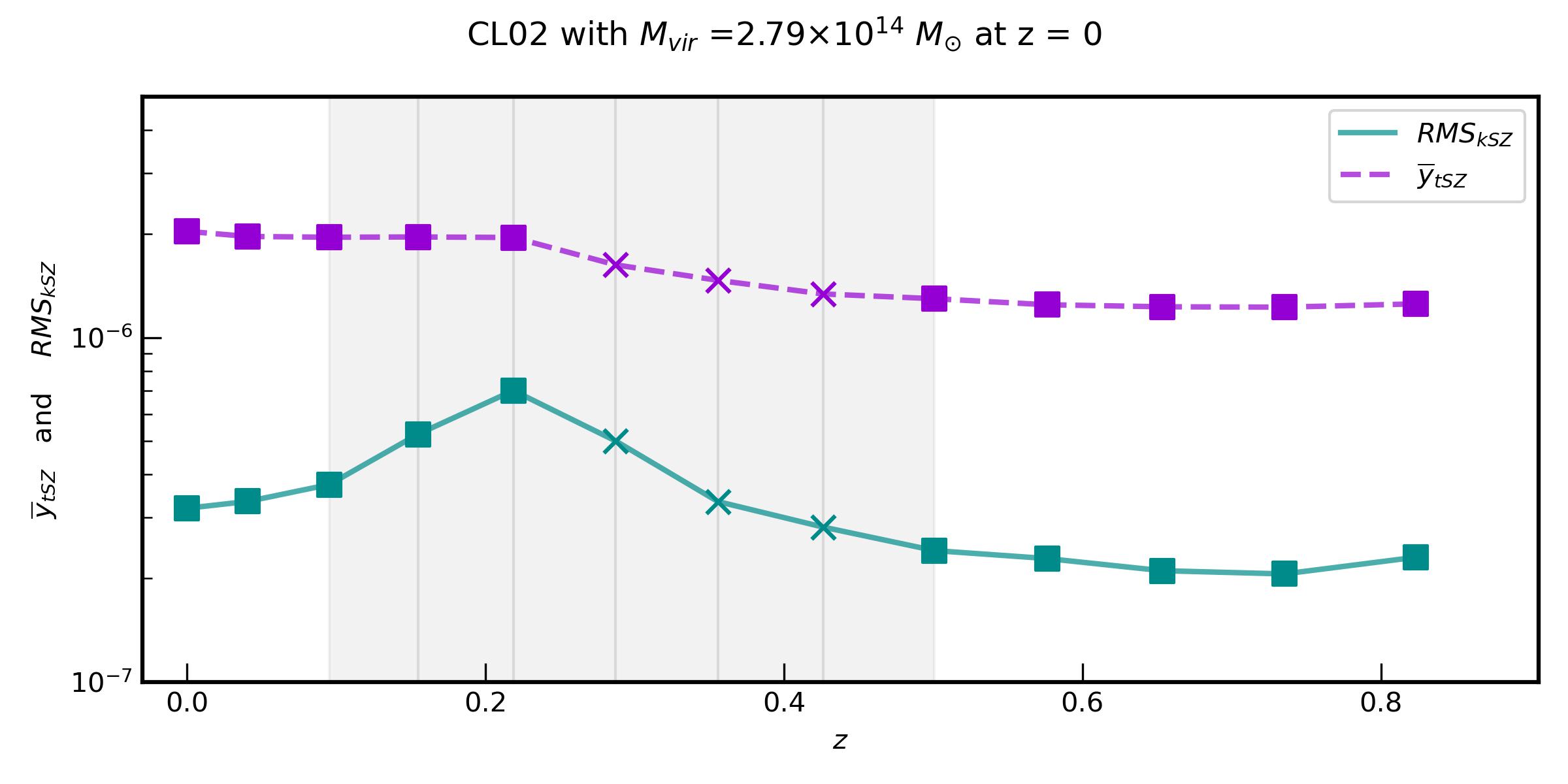
In the first case, CL01 suffers a major merger at , which rises the kSZ and tSZ signals. Once the merger phase ends at it becomes marginally relaxed and, in the end, relaxed, decreasing its kSZ signal but maintaining the tSZ nearly constant or even increasing it, due to the mass growth. In the second case, CL02 starts with a major merger at , being thus an unrelaxed cluster. Once this period ends, it becomes marginally relaxed, reducing the kSZ signal until , where it enters a minor merger period, becomes unrelaxed and increases both, the thermal and kinetic signals. In the end, when it becomes again marginally relaxed, the kSZ effect decreases but the tSZ remains constant.
Both study cases reassert the correlation between the cluster dynamical state (including mergers) and the kinetic part of the SZ signal. During merging periods (unrelaxed), the kSZ signal increases, while in quiescent periods (relaxed), it decreases. Simultaneously, the tSZ signal rises during merging periods due to mass gain and heating by compression and merger shocks, but does not decrease in relaxed periods. Therefore, in line with Fig. 3, we can anticipate that, for the same mass, unrelaxed clusters should generally exhibit a more pronounced kSZ signal than the relaxed population, while the tSZ effect is minimally affected by this classification.
We can also highlight the thin line that can exist between our marginally relaxed an unrelaxed population with these particular clusters. Although CL01 only presents a marginally relaxed dynamical state once it ends the merging periods, CL02 exhibits this state even at the peak of the kSZ signal at , from which it starts to decrease. Hence, despite the fact that the marginally relaxed state appears in quiescent periods and at the end of merger or high accretion epochs, clusters can be significantly disturbed in this state. That is one of the main reasons why we predominantly highlight the differences between relaxed and unrelaxed populations in all the previous results, putting the marginally relaxed systems in a second plane, since they are halfway of the other dynamical states and can blur the main differences between them.
4 Summary and conclusions
The main goal of this work is to assess the correlation between GCs dynamical state and their associated SZ signals, both thermal and kinetic. To do so, a sample of cluster-like haloes extracted from a cosmological AMR simulation is used. The SZ effect strongly depends on density, temperature and velocity distributions of the baryonic component of such haloes. Therefore, those events able to substantially alter these quantities and, thus, changing the cluster dynamical state (e.g. mergers, accretion, etc.), would be crucial to establish the previously mentioned correlation.
We have defined three main dynamical state classes, according to Vallés-Pérez et al. (2023), and have primarily focused on the clearly differentiate cases of relaxed and unrelaxed (or disturbed) clusters, in order to maximise the main differences. Hence, at fixed redshift, we obtain the following results:
-
•
The kinetic part of the effect shows a strong correlation with cluster dynamical state. Disturbed clusters present an overall higher kSZ signal for all masses than the relaxed population and a steeper trend with mass ( for disturbed vs for relaxed systems). This would be mostly explained by the fact that the unrelaxed sample has an overall higher velocity dispersion () and, hence, the kinetic pressure plays an important role in the cluster dynamics. On the other hand, the relaxed population would be mostly supported by thermal pressure and, therefore, uncorrelated to the kinetic signal.
-
•
Correlation between gas angular momentum and the kSZ effect is only evident among relaxed clusters, as the signal in disturbed objects would be dominated by turbulence and non-rotational motions. By means of a multipole expansion on the kSZ maps, it becomes apparent that, overall, the dipole constitutes the most significant component of the effect, particularly within the relaxed sample. This characteristic can be leveraged by stacking multiple, appropriately oriented, and centred kSZ maps, allowing the retrieval of a dipole-like signal that correlates with the global rotation properties of the cluster sample.
-
•
The thermal component lacks a robust correlation with cluster dynamical state, primarily because it is unaffected by the baryonic velocity distribution. However, the radial profiles presented seem to indicate that unrelaxed clusters exhibit a more flattened trend, while the relaxed sample displays greater concentration towards the cluster centre. This has been confirmed by observations in Adam et al. (2023).
Our haloes at can be traced backwards in cosmic time using the ASOHF merger tree. Hence, for each simulation snapshot we have recovered the cluster dynamical state history, together with the minor and major mergers suffered. Joining this information with the thermal and kinetic SZ signals of every cluster at all cosmic epochs we can infer that, during merging periods, when the cluster is disturbed, the kinetic part of the SZ effect rises, while in quiescent periods it decreases. The tSZ signal, however, does not decrease once the disturbed phase is over and thus, it seems to be almost independent of the cluster dynamical state.
Based on our findings, the kSZ effect opens a new window of opportunity to assess the dynamical state of clusters, particularly in distinguishing clusters undergoing a quiescent evolution from those marked by a history of significant merging events. Consequently, our results suggest that upcoming observational data, focused on measuring the SZ effect in clusters, could serve as a valuable complementary approach to describe the evolution of galaxy clusters. Additionally, and especially in cases where clusters exhibit a relaxed state, our analysis suggests that the kSZ effect holds potential for estimating dynamical quantities such as the gas rotation.
Acknowledgements.
This work has been supported by the Agencia Estatal de Investigación Española (AEI; grant PID2022-138855NB-C33), by the Ministerio de Ciencia e Innovación (MCIN) within the Plan de Recuperación, Transformación y Resiliencia del Gobierno de España through the project ASFAE/2022/001, with funding from European Union NextGenerationEU (PRTR-C17.I1), and by the Generalitat Valenciana (grant PROMETEO CIPROM/2022/49). OM and DV acknowledge support from Universitat de València through Atracció de Talent fellowships. Simulations have been carried out using the supercomputer Lluís Vives at the Servei d’Informàtica of the Universitat de València.References
- Adam et al. (2017) Adam, R., Bartalucci, I., Pratt, G., et al. 2017, Astronomy & Astrophysics, 598, A115
- Adam et al. (2023) Adam, R., Ricci, M., Eckert, D., et al. 2023, The XXL Survey LV. Pressure profile and - scaling relation in three low-mass galaxy clusters at observed with NIKA2
- Ade et al. (2014) Ade, P. A., Aghanim, N., Armitage-Caplan, C., et al. 2014, Astronomy & Astrophysics, 571, A29
- Alfano et al. (2023) Alfano, A. C., Luongo, O., & Muccino, M. 2023, arXiv preprint arXiv:2311.05324
- Altamura et al. (2023) Altamura, E., Kay, S. T., Chluba, J., & Towler, I. 2023, Monthly Notices of the Royal Astronomical Society, stad1841
- Amodeo et al. (2021) Amodeo, S., Battaglia, N., Schaan, E., et al. 2021, Phys. Rev. D, 103, 063514
- Baldi et al. (2018) Baldi, A. S., De Petris, M., Sembolini, F., et al. 2018, Monthly Notices of the Royal Astronomical Society, 479, 4028
- Battaglia et al. (2017) Battaglia, N., Ferraro, S., Schaan, E., & Spergel, D. N. 2017, Journal of Cosmology and Astroparticle Physics, 2017, 040
- Baxter et al. (2019) Baxter, E. J., Sherwin, B. D., & Raghunathan, S. 2019, Journal of Cosmology and Astroparticle Physics, 2019, 001
- Birkinshaw (1999) Birkinshaw, M. 1999, Physics Reports, 310, 97
- Bryan & Norman (1998) Bryan, G. L. & Norman, M. L. 1998, The Astrophysical Journal, 495, 80
- Bullock et al. (2001) Bullock, J. S., Dekel, A., Kolatt, T. S., et al. 2001, The Astrophysical Journal, 555, 240
- Carlstrom et al. (2002) Carlstrom, J. E., Holder, G. P., & Reese, E. D. 2002, Annual Review of Astronomy and Astrophysics, 40, 643
- Chen et al. (2022) Chen, Z., Zhang, P., Yang, X., & Zheng, Y. 2022, Monthly Notices of the Royal Astronomical Society, 510, 5916
- Chluba & Mannheim (2002) Chluba, J. & Mannheim, K. 2002, Astronomy & Astrophysics, 396, 419
- Cimatti et al. (2019) Cimatti, A., Fraternali, F., & Nipoti, C. 2019, Introduction to galaxy formation and evolution: from primordial gas to present-day galaxies (Cambridge University Press)
- Colafrancesco (2007) Colafrancesco, S. 2007, New Astronomy Reviews, 51, 394
- Cooray & Chen (2002) Cooray, A. & Chen, X. 2002, The Astrophysical Journal, 573, 43
- Cui et al. (2018) Cui, W., Knebe, A., Yepes, G., et al. 2018, Monthly Notices of the Royal Astronomical Society, 480, 2898
- Diemer (2018) Diemer, B. 2018, The Astrophysical Journal Supplement Series, 239, 35
- Dupke & Bregman (2002) Dupke, R. A. & Bregman, J. N. 2002, The Astrophysical Journal, 575, 634
- Eisenstein & Hu (1998) Eisenstein, D. J. & Hu, W. 1998, ApJ, 496, 605
- Gouin et al. (2020) Gouin, C., Aghanim, N., Bonjean, V., & Douspis, M. 2020, Astronomy & Astrophysics, 635, A195
- Haardt & Madau (1995) Haardt, F. & Madau, P. 1995, arXiv preprint astro-ph/9509093
- Hand et al. (2012) Hand, N., Addison, G. E., Aubourg, E., et al. 2012, Physical Review Letters, 109, 041101
- Hasselfield et al. (2013) Hasselfield, M., Hilton, M., Marriage, T. A., et al. 2013, Journal of Cosmology and Astroparticle Physics, 2013, 008
- Hernández-Monteagudo et al. (2015) Hernández-Monteagudo, C., Ma, Y.-Z., Kitaura, F. S., et al. 2015, Physical Review Letters, 115, 191301
- Hill et al. (2016) Hill, J. C., Ferraro, S., Battaglia, N., Liu, J., & Spergel, D. N. 2016, Physical Review Letters, 117, 051301
- Hockney & Eastwood (1988) Hockney, R. W. & Eastwood, J. W. 1988, Computer simulation using particles
- Knebe et al. (2011) Knebe, A., Knollmann, S. R., Muldrew, S. I., et al. 2011, MNRAS, 415, 2293
- Kompaneets (1957) Kompaneets, A. 1957, Soviet Journal of Experimental and Theoretical Physics, 4, 730
- Lokken et al. (2023) Lokken, M., Cui, W., Bond, J. R., et al. 2023, Monthly Notices of the Royal Astronomical Society, 523, 1346
- Mallaby-Kay et al. (2023) Mallaby-Kay, M., Amodeo, S., Hill, J. C., et al. 2023, Phys. Rev. D, 108, 023516
- Matilla & Haiman (2020) Matilla, J. M. Z. & Haiman, Z. 2020, Physical Review D, 101, 083016
- Mroczkowski et al. (2019) Mroczkowski, T., Nagai, D., Basu, K., et al. 2019, Space Science Reviews, 215, 1
- Penzias & Wilson (1979) Penzias, A. A. & Wilson, R. W. 1979, in A Source Book in Astronomy and Astrophysics, 1900–1975 (Harvard University Press), 873–876
- Plagge et al. (2013) Plagge, T. J., Marrone, D. P., Abdulla, Z., et al. 2013, The Astrophysical Journal, 770, 112
- Planck Collaboration et al. (2013) Planck Collaboration, P., Ade, P., Aghanim, N., et al. 2013, ArXiv e-prints, 1303, 5080
- Planck Collaboration et al. (2020) Planck Collaboration, P., Aghanim, N., Akrami, Y., et al. 2020
- Planelles et al. (2017) Planelles, S., Fabjan, D., Borgani, S., et al. 2017, Monthly Notices of the Royal Astronomical Society, 467, 3827
- Planelles et al. (2018) Planelles, S., Mimica, P., Quilis, V., & Cuesta-Martínez, C. 2018, Monthly Notices of the Royal Astronomical Society, 476, 4629
- Planelles & Quilis (2010) Planelles, S. & Quilis, V. 2010, Astronomy & Astrophysics, 519, A94
- Quilis (2004) Quilis, V. 2004, MNRAS, 352, 1426
- Quilis et al. (2020) Quilis, V., Martí, J.-M., & Planelles, S. 2020, MNRAS, 494, 2706
- Reichardt et al. (2013) Reichardt, C., Stalder, B., Bleem, L., et al. 2013, The Astrophysical Journal, 763, 127
- Rephaeli (1995) Rephaeli, Y. 1995, Annual review of astronomy and astrophysics, 33, 541
- Sarazin (1988) Sarazin, C. 1988, Sky and Telescope, 76, 639
- Sayers et al. (2013) Sayers, J., Mroczkowski, T., Zemcov, M., et al. 2013, The Astrophysical Journal, 778, 52
- Schaan et al. (2021) Schaan, E., Ferraro, S., Amodeo, S., et al. 2021, Physical Review D, 103, 063513
- Schaan et al. (2016) Schaan, E., Ferraro, S., Vargas-Magana, M., et al. 2016, Physical Review D, 93, 082002
- Schneider & Bartelmann (1997) Schneider, P. & Bartelmann, M. 1997, Monthly Notices of the Royal Astronomical Society, 286, 696
- Simionescu et al. (2019) Simionescu, A., ZuHone, J., Zhuravleva, I., et al. 2019, Space Science Reviews, 215, 1
- Soergel et al. (2016) Soergel, B., Flender, S., Story, K., et al. 2016, Monthly Notices of the Royal Astronomical Society, 461, 3172
- Springel et al. (2001) Springel, V., White, M., & Hernquist, L. 2001, ApJ, 549, 681
- Sunyaev & Zeldovich (1980) Sunyaev, R. & Zeldovich, Y. B. 1980, Monthly Notices of the Royal Astronomical Society, vol. 190, Feb. 1980, p. 413-420., 190, 413
- Tinker et al. (2008) Tinker, J., Kravtsov, A. V., Klypin, A., et al. 2008, The Astrophysical Journal, 688, 709
- Vallés-Pérez et al. (2023) Vallés-Pérez, D., Planelles, S., Monllor-Berbegal, Ó., & Quilis, V. 2023, Monthly Notices of the Royal Astronomical Society, 519, 6111
- Vallés-Pérez et al. (2020) Vallés-Pérez, D., Planelles, S., & Quilis, V. 2020, Monthly Notices of the Royal Astronomical Society, 499, 2303
- Vallés-Pérez et al. (2021a) Vallés-Pérez, D., Planelles, S., & Quilis, V. 2021a, Monthly Notices of the Royal Astronomical Society, 504, 510
- Vallés-Pérez et al. (2021b) Vallés-Pérez, D., Planelles, S., & Quilis, V. 2021b, Computer Physics Communications, 263, 107892
- Vallés-Pérez et al. (2022) Vallés-Pérez, D., Planelles, S., & Quilis, V. 2022, Astronomy & Astrophysics, 664, A42
- Vazza et al. (2017) Vazza, F., Jones, T. W., Brüggen, M., et al. 2017, Monthly Notices of the Royal Astronomical Society, 464, 210
- Voit (2005) Voit, G. M. 2005, Reviews of Modern Physics, 77, 207
- Xia et al. (2021) Xia, Q., Neyrinck, M. C., Cai, Y.-C., & Aragón-Calvo, M. A. 2021, Monthly Notices of the Royal Astronomical Society, 506, 1059
- Zeldovich & Sunyaev (1969) Zeldovich, Y. B. & Sunyaev, R. 1969, Astrophysics and Space Science, 4, 301