Altermagnetism and superconductivity in a multiorbital $t$-$J$ model

Abstract

Motivated by exploring doped multi-orbital antiferromagnets (AFMs) and altermagnets ($A\ell M$s) we explore minimal $t$-$J$ models on the square-octagon lattice which favor such collinear magnetic orders in the regime where spin exchange dominates. While the AFM order breaks translational and time-reversal symmetries, the $A\ell M$ state (equivalently, a ‘$d$-wave ferromagnet’) features multipolar order which separately breaks time-reversal and crystal rotation symmetries but preserves their product leading to spin-split bands with zero net magnetization. We study the mean field phase diagram of these models as we vary doping and interactions, discovering regimes of weak and strong $A\ell M$ order, superconductivity including uniform $s$-wave and $d$-wave pairing states, incipient $d$-wave pair density wave order, and phases with coexisting singlet-triplet pairing and AFM/$A\ell M$ orders which appear unstable to phase separation and could host stripe order with longer-range interactions. Our results may be relevant to doping or pressure studies of multiorbital $A\ell M$ materials.

I Introduction

The one-band Hubbard and $tJ$ models have been extensively investigated following the discovery of high temperature cuprate superconductivity [1, 2, 3, 4]. These models are thought to capture the physics of a wide variety of correlated superconductors which descend from nearby states with Mott insulating antiferromagnetic order or other collinear spin density wave orders [3, 5, 6, 7, 8]. Indeed, fluctuating magnetism is thought to be the ‘pairing glue’ responsible for unconventional superconductivity [9, 10, 11, 12]. In this context it is interesting to explore the effect of doping on materials with more complex collinear magnetic orders such as the recently discovered altermagnet ($A\ell M$) order [13, 14]. Altermagnets are naturally multi-orbital systems, which host magnetic order that is akin to a type of multipolar order [15]. $A\ell M$s preserve translational symmetry unlike AFMs. While they break time-reversal and lattice rotation symmetries, they preserve the product of these two symmetries which leads to zero net magnetization while still hosting spin-split bands [16, 17]. This makes $A\ell M$s of potential interest for spintronic applications [18, 19]. and several candidate materials such as CrSb [20], Mn₅Si₃ [21], MnTe [22], $\kappa$-Cl [23], and many others have been experimentally explored. Recent work has explore the Landau theory of altermagnets [24], their symmetry classification and their nodal excitations [25, 26, 27], and coupling of magnetism to phonons [24, 28]. Electrons which are proximity coupled to magnetic fluctuations in such altermagnets can potentially form $p$-wave triplet superconductors [29, 30, 31, 32], while proximity coupling of $A\ell M$ to conventional superconducting states could support topological superconductivity with edge or corner Majorana modes [33]. In this context, it is interesting to explore possible superconductivity in doped or pressurized $A\ell M$ ordered materials.

A second important ingredient of superconductivity in many of the correlated quantum materials is that they exhibit multiple bands, at or near the Fermi level, which emerge from multiple atomic orbitals or multiple atoms in the unit cell. Such multiorbital models are important for a careful microscopic modelling of the CuO₂ layers in the cuprate superconductors [34, 35, 36, 37, 38, 39, 40], and play a more direct role in superconductors like Sr₂RuO₄ [41, 42, 43, 44] and the more recently discovered iron-based [45] and nickel-based high temperature superconductors [46, 47, 48, 49, 50, 51, 52, 53, 54]. Multi-orbital models also leads to a more natural description of the rich variety of orders found generically in these systems including stripe and nematic orders [55, 56, 57, 58]. It is thus interesting to ask if multiorbital systems can also more naturally host unusual superconductivity associated with nonzero-momentum pairing called ‘pair density wave order’ which have been found in numerical studies of simple phenomenological models [59, 60, 61, 62, 63, 64].

Motivated by both the above sets of observations, our work in this paper explores $tJ$ models in a multiorbital system. We consider a square-octagon lattice model [65, 66, 67] which can support either AFM or $A\ell M$ order depending on the sign of certain exchange interactions. The simplest $A\ell M$ order which we will consider in this paper may also be termed a $d$-wave ferromagnet. Starting with this model, we study the effect of doping and interactions in such $tJ$ models using mean field theory, exploring both uniform symmetry broken states as well as possible spatially modulated orders. Our main result is that the resulting phase diagram contains a rich plethora of phases which include strong AFM/$A\ell M$ insulators, states with weak $A\ell M$ order or $d$-wave spin density wave states induced by quasi-one-dimensional van Hove singularities, and $s$-wave and $d$-wave paired superconductors. We also find regimes of incipient $d$-wave pair density wave states over a range of densities at weak coupling, which could potentially be stabilized with additional nonlocal interactions. In addition, we find states where AFM/$A\ell M$ order coexists with $d$-wave superconductivity leading to mixed singlet-triplet pairing, which however appear unstable to phase separation into droplets with Mott insulating AFM/$A\ell M$ order and droplets with $d$-wave superconductivity - these may form more organized structures (e.g., stripes) in the presence of longer range interactions.

II Multi-orbital Model

We consider a decorated square lattice model with four sites per unit cell as depicted in Fig. 1. The Hamiltonian we study is

$$\!\!H=-\!\!\!\sum_{\langle i,j\rangle,\sigma}\!\!t_{ij}(c^{\dagger}_{i\sigma}c^{\phantom{\dagger}}_{j\sigma}\!+\!{\rm h.c.})\!+\!\!\sum_{\langle i,j\rangle}J_{ij}\mathbf{S}_{i}\!\cdot\!\mathbf{S}_{j}\!-\!\mu\!\sum_{i}n^{\phantom{\dagger}}_{i\sigma}$$ (1)

Here, the intra-cell and inter-cell nearest-neighbor hoppings are $t_{ij}=t_{1}$ and $t_{ij}=t_{2}$ respectively, and the corresponding spin exchange couplings on those bonds are denoted by $J_{ij}=J_{1}$ and $J_{ij}=J_{2}$ respectively. We set $t_{1}=1$ to define the unit of energy, fix parameters $t_{2}/t_{1}=1/2$, consider different $J_{2}/J_{1}$, and tune the electron filling $0<\bar{n}<1$ and interaction strength $J_{1}/t_{1}$. $\bar{n}=1$ corresponds to $8$ electrons per unit cell. While the $J_{2}>0$ arises naturally from a Hubbard model, the case $J_{2}<0$ can only arise from additional Hund’s coupling physics with multiple on-site orbitals, so we view it here only as a convenient model Hamiltonian to capture $A\ell M$ order in this example. Furthermore, we are not implementing strict Gutzwiller projection of the electrons - we may view these $tJ$ models as having renormalized hopping and interactions in the spirit of ‘renormalized mean field theory’ [4], or simply as toy models to explore magnetic and pairing instabilities driven by exchange interactions within unrestricted Hartree-Fock-Bogoliubov theory in the spirit of earlier work on the one-band model for cuprates [68].

This Hamiltonian has lattice symmetries including translation, a $\mathcal{C}_{4}$ rotation around the center of the squares, inversion $\mathcal{I}$ around the center of the squares and octagons, four mirror symmetries $\mathcal{M}$, and time-reversal $\mathcal{T}$. The symmetries of the Hamiltonian also include internal symmetries like $SU(2)$ spin rotation, and a particle-hole symmetry.

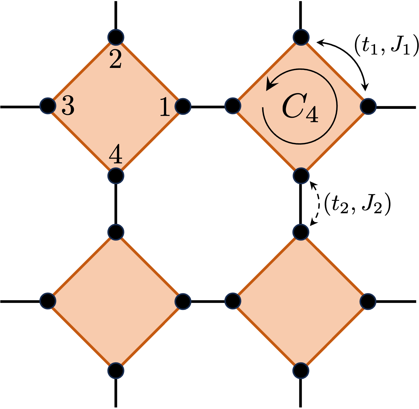
Figure 1: Decorated square lattice model, also known as the square-octagon lattice, with four-site unit cell. The intra-cell hopping and spin exchange are denoted by $(t_{1},J_{1})$, and inter-cell hopping and spin exchange are denoted by $(t_{2},J_{2})$. We set $t_{1}\!=\!1$, $t_{2}\!=\!t_{1}/2$, and $J_{2}/J_{1}\!=\!-J/4$. We vary the electron filling $\bar{n}$ and interaction $J_{1}/t$, keeping $J_{1}\!>\!0$.

II.1 Orbital basis

In the absence of interactions, it is useful to solve the single unit cell in terms of “orbitals”. We label each site $i$ in terms of unit cell position $\mathbf{r}$ and basis $\ell=1$-$4$. Using this, the orbitals correspond to

$$s_{\mathbf{r}\sigma} = \frac{1}{2}(c_{\mathbf{r}1\sigma}+c_{\mathbf{r}2\sigma}+c_{\mathbf{r}3\sigma}+c_{\mathbf{r}4\sigma})$$ (2)

$$d_{\mathbf{r}\sigma} = \frac{1}{2}(c_{\mathbf{r}1\sigma}-c_{\mathbf{r}2\sigma}+c_{\mathbf{r}3\sigma}-c_{\mathbf{r}4\sigma})$$ (3)

$$X_{\mathbf{r}\sigma} = \frac{1}{\sqrt{2}}(c_{\mathbf{r}1\sigma}-c_{\mathbf{r}3\sigma})$$ (4)

$$Y_{\mathbf{r}\sigma} = \frac{1}{\sqrt{2}}(c_{\mathbf{r}2\sigma}-c_{\mathbf{r}4\sigma})$$ (5)

which are respectively $s$-orbital, $d$-orbital, and a pair of degenerate $p$-orbitals $X,Y$. The corresponding energies for a single unit cell are $\varepsilon_{s}=-2t_{1}$, $\varepsilon_{X}=\varepsilon_{Y}=0$, $\varepsilon_{d}=+2t_{1}$. These orbitals will form corresponding bands, which for $t_{2}\ll t_{1}$ are non-overlapping. In this case, with increasing filling, we go from filling the $s$-orbital band, to the $X,Y$-orbital bands, and eventually the $d$-orbital band, with gapped band insulators appearing in between when some of these bands are filled.

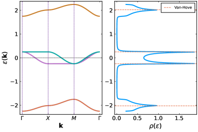
Figure 2: (left) Band structure of the multi-orbital model studied, showing the $s$ (low energy), $p_{x}$/$p_{y}$ (intermediate energy), and $d$ (high energy) bands along high symmetry path $\Gamma$-$X$-$M$. The gap between the bands $\sim 2t_{1}$, which is evident from the single unit-cell solution. (right) Density of states (DOS) of the non-interacting multi-orbital model. In addition to the $s$-$p$ and $p$-$d$ band gaps, the DOS shows 2D van Hove singularity (vHS) in the $s$-band ($d$-band) bands at filling $n\sim 0.125$ ($n\sim 0.875$) as well as quasi-1D $p$-band vHS at $n\sim 0.26,0.74$.

II.2 Fermi surfaces

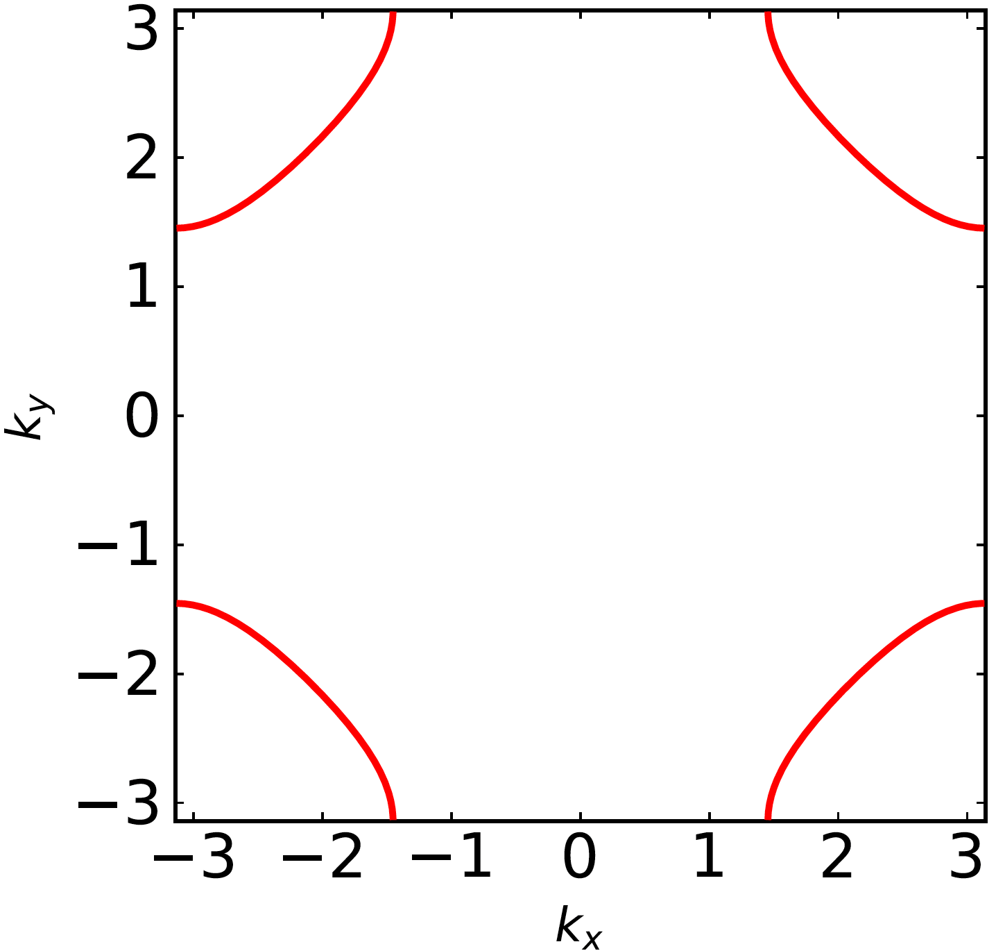
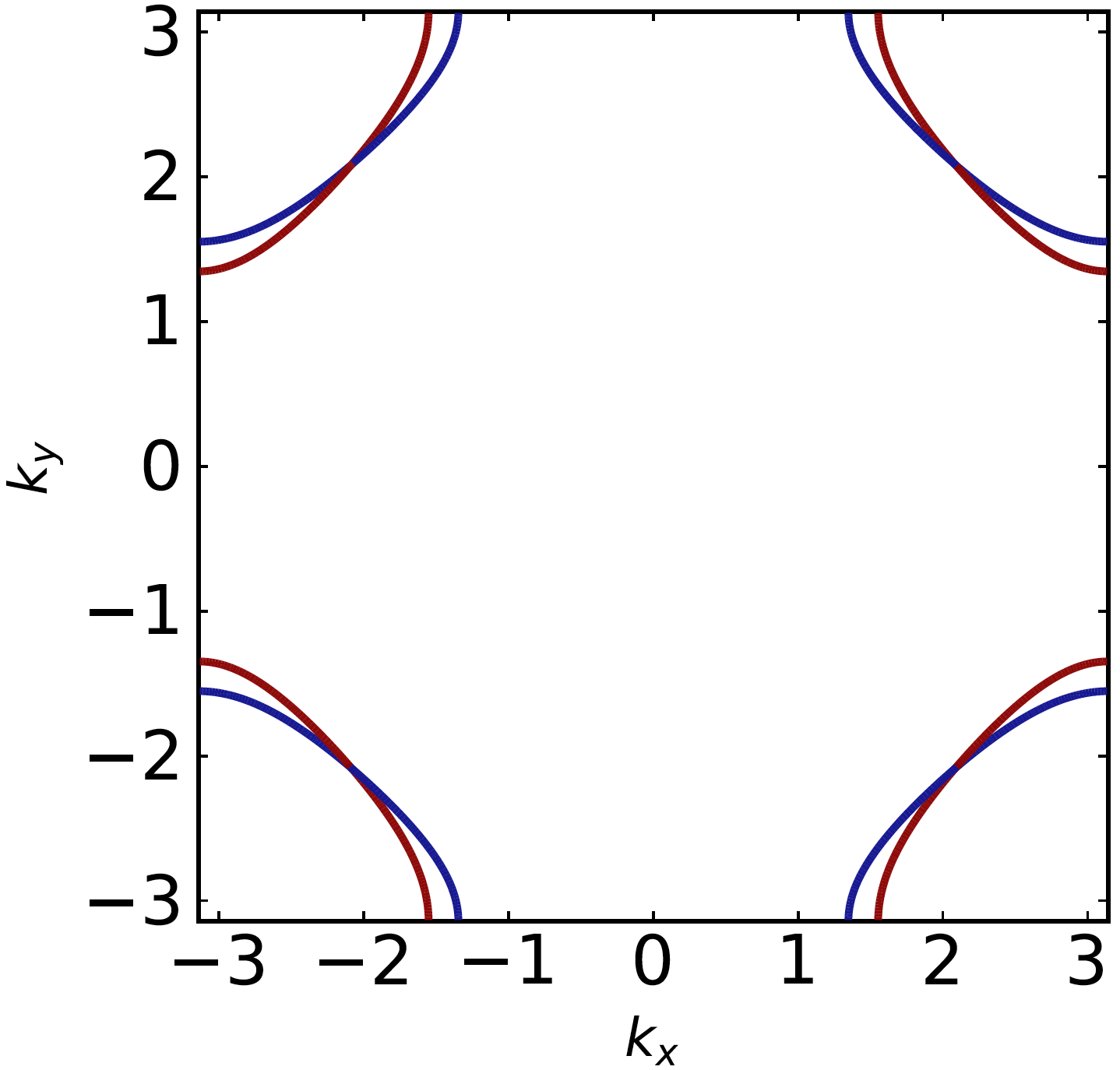
Figure 3: Hole-like Fermi surfaces at $\bar{n}=0.2$ filling where the $s$-orbital band, with dispersion minimum at the $\Gamma$ point, is more than half-filled. Left: In the absence of altermagnet order, with spin degenerate FSs. Right: In the presence of altermagnet order with the coloring of the bands indicating the spin polarization.

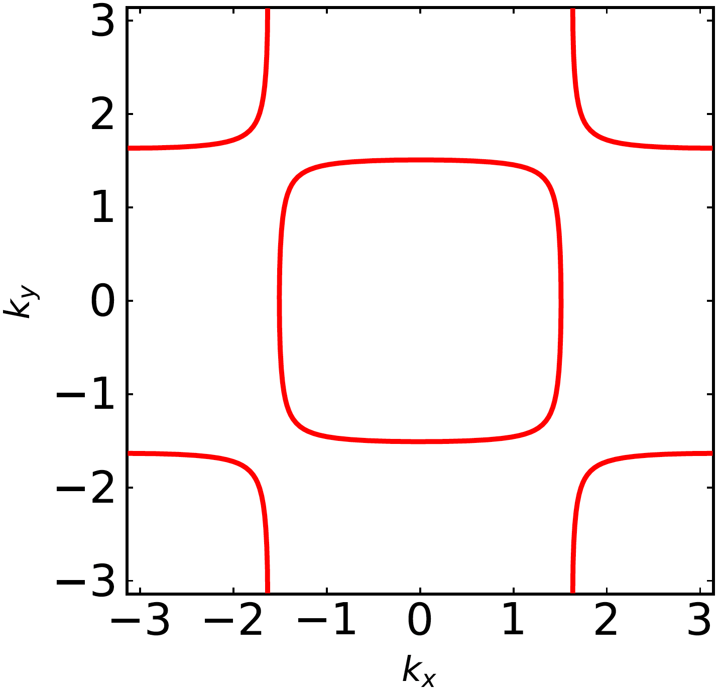
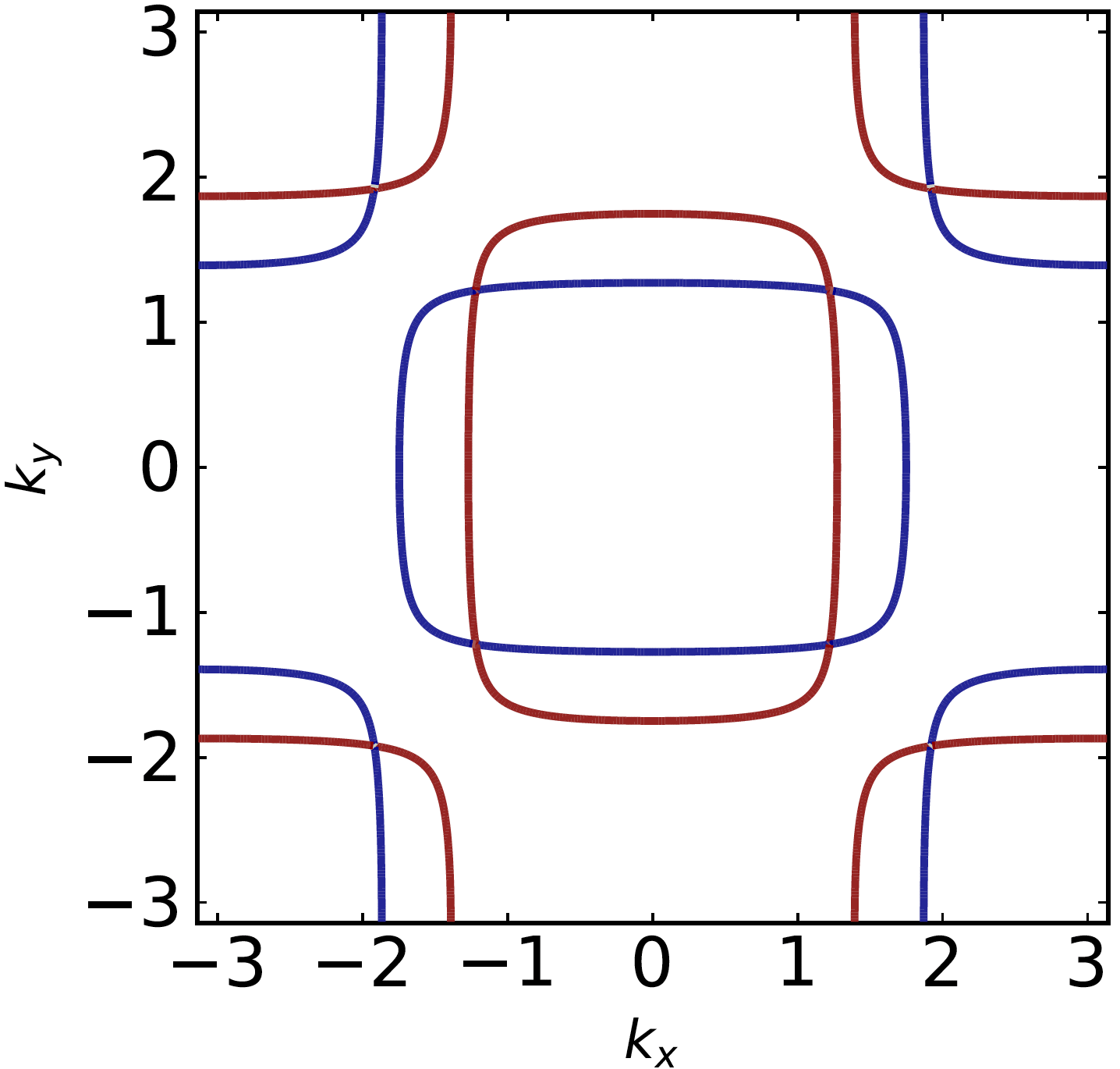
Figure 4: Fermi surfaces at $\bar{n}$=0.5 filling where the $p_{x},p_{y}$ orbital bands are partially occupied. Left: In the absence of altermagnet order, with spin degenerate FSs. Right: In the presence of altermagnet order with the coloring of the bands indicating the spin polarization.

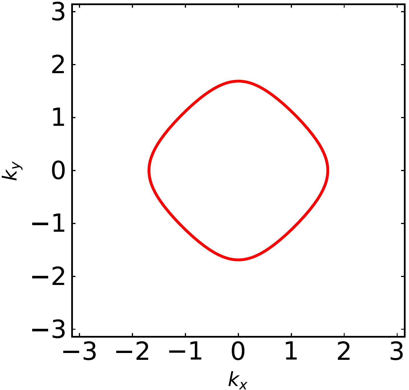
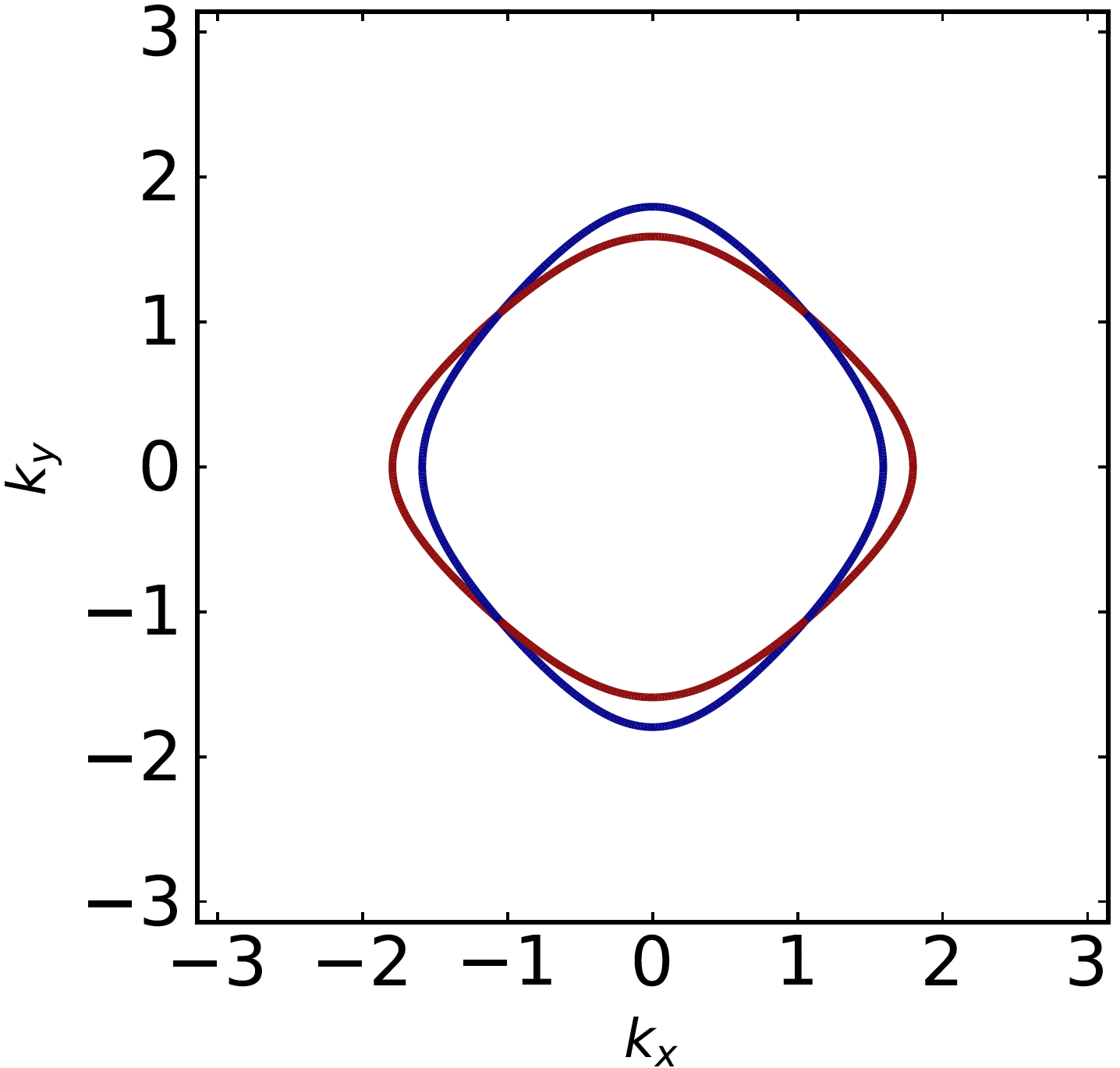
Figure 5: Electron-like Fermi surfaces at $\bar{n}$=0.8 filling where the $d$-orbital band is partially occupied. Left: In the absence of altermagnet order, with spin degenerate FSs. Right: In the presence of weak altermagnet order with the coloring of the bands indicating the spin polarization.

II.2.1 Low filling

The spin-degenerate Fermi surfaces of the full $8$-band model (including spin) shown in Fig. 3 (left) at a filling $\bar{n}=0.2$. To understand this, we note that for fillings $\bar{n}<0.25$, the partially occupied bands arise from the $s$-orbitals as given in (2). This leads to an effective $s$-orbitals hopping Hamiltonian which resembles a simple square lattice with nearest-neighbour hopping $t_{2}$, with an effective Hamiltonian

$$H^{\rm eff}_{s} = \!\!\sum_{{{\bf{k}}}}\!\varepsilon^{s}_{{\bf{k}}}s^{\dagger}_{{{\bf{k}}}\sigma}s^{\phantom{\dagger}}_{{{\bf{k}}}\sigma}$$ (6)

$$\varepsilon^{s}_{{\bf{k}}} = -2t_{1}-\frac{t_{2}}{2}(\cos k_{x}+\cos k_{y})$$ (7)

which has a minimum at the Brillouin zone (BZ) center $\Gamma=(0,0)$ point. The filling of the $s$-band corresponds to $n^{\rm eff}_{s}=4\bar{n}$, so that the FS in Fig. 3 with $\bar{n}=0.2$ corresponds to $n^{\rm eff}_{s}=0.8$. When we add some altermagnetic order, captured by a translationally invariant but basis-site dependent magnetic field in the unit cell which takes on value $+h$ (or $-h$) for basis sites $1,3$ (respectively $2,4)$, we find spin-splitting of the FSs as shown in Fig. 3 (right). In addition, there are four ‘$d$-wave’ nodes where the spin-up and spin-down Fermi-surfaces touch at four points on the $k_{x}=\pm k_{y}$ lines. This degeneracy is consistent with the fact that the altermagnet has $x,y$ spatial mirror symmetries and preserves $\mathcal{T}\otimes\mathcal{C}_{4}$.

II.2.2 Intermediate filling

Fig. 4 shows the FSs at intermediate filling, $1/4<\bar{n}<1/2$. For fillings $0.25<\bar{n}<0.75$, the bands can be effectively described in terms of an effective hopping Hamiltonian arising from $X$ and $Y$ orbitals hopping along their easy axis ($x$ and $y$) respectively. This leads to a

$$H^{\rm eff}_{p} = \!\!\sum_{{{\bf{k}}}}\!\left[\varepsilon^{X}_{{\bf{k}}}X^{\dagger}_{{{\bf{k}}}\sigma}X^{\phantom{\dagger}}_{{{\bf{k}}}\sigma}\!+\!\varepsilon^{Y}_{{\bf{k}}}Y^{\dagger}_{{{\bf{k}}}\sigma}Y^{\phantom{\dagger}}_{{{\bf{k}}}\sigma}\right.$$ (8)

$$+ \!\left.\varepsilon^{XY}_{{\bf{k}}}(X^{\dagger}_{{{\bf{k}}}\sigma}Y^{\phantom{\dagger}}_{{{\bf{k}}}\sigma}\!+\!{\rm h.c.})\right]$$

where $\varepsilon^{X}_{{\bf{k}}}=t_{2}\cos k_{x}$, $\varepsilon^{Y}_{{\bf{k}}}=t_{2}\cos k_{y}$, and an orbital mixing term with $\varepsilon^{XY}_{{\bf{k}}}=t^{\prime}\sin k_{x}\sin k_{y}$. Direct projection does not lead to this orbital mixing term, but it is generated by perturbative processes which virtually excite to the $s,d$ orbitals so that $t^{\prime}\approx t_{2}^{2}/2t_{1}$.

The resulting FSs are shown in Fig. 4 without and with $A\ell M$ order. In the absence of $A\ell M$ order, we find two FS pockets, one centered at the $\Gamma=(0,0)$ point and the other at $(\pi,\pi)$. The electron number (for each spin) in these bands goes from $n^{\rm eff}_{p}({{\bf{k}}})=0$ in the BZ center, to $n^{\rm eff}_{p}({{\bf{k}}})=1$ as we cross one FS, and to $n^{\rm eff}_{p}=2$ as we cross the second FS. With $A\ell M$ order, both FS pockets get spin split with $8$ band touching points along the $k_{x}=\pm k_{y}$ lines.

II.2.3 High filling

The simple model we have considered is particle-hole symmetric, invariant under $c^{\phantom{\dagger}}_{\mathbf{r},i,\sigma}\to(-1)^{\mathbf{r}_{x}+\mathbf{r}_{y}}c^{\dagger}_{\mathbf{r},i,\sigma}$. This leads to a momentum dispersion for the high energy $d$-orbital derived bands at large filling $\bar{n}$, to be the same as the $s$-orbital band dispersion at low filling $1-\bar{n}$ except for a shift in momentum by $(\pi,\pi)$. Fig. 5 shows these FSs for $\bar{n}=0.8$ without and with $A\ell M$ order.

II.3 Projected Hamiltonians

We can simplify the full interacting Hamiltonians by projecting to specific orbitals at various fillings. For low filling, $0<\bar{n}<1/4$, we can project to the $s$-orbital. At intermediate filling, $1/4<\bar{n}<3/4$, the physics is governed by the $X,Y$-orbitals. Finally, at high fillings, $3/4<\bar{n}<1$, we project to $d$-orbital states. Since the Hamiltonian has particle-hole symmetry, the physics in the $s$-orbital dominated regime at low filling $\bar{n}<1/4$ is the same as the $d$-orbital regime at high filling $1-\bar{n}<1/4$. These simplified models will be useful for interpreting our full numerical mean field results discussed in the following section.

II.3.1 Low/High filling

For $\bar{n}<1/4$, we invert the above equations Eq. 2 and then project to the $s$-orbital, which we can account for by setting $c_{\mathbf{r}\ell\sigma}\to s_{\mathbf{r}}/2$ for all sublattices $\ell=1$-$4$. Using this, we find

$$H = -\frac{t_{2}}{4}\!\!\sum_{\langle\mathbf{r},\mathbf{r}^{\prime}\rangle,\sigma}(s^{\dagger}_{\mathbf{r}\sigma}s^{\phantom{\dagger}}_{\mathbf{r}^{\prime}\sigma}+{\rm h.c.})\!-\!\mu\!\sum_{\mathbf{r}\sigma}s^{\dagger}_{\mathbf{r}\sigma}s^{\phantom{\dagger}}_{\mathbf{r}\sigma}$$ (9)

$$- \frac{3J_{1}}{8}\sum_{\mathbf{r}}n^{(s)}_{\mathbf{r}\uparrow}n^{(s)}_{\mathbf{r}\downarrow}+\frac{J_{2}}{16}\sum_{\langle\mathbf{r},\mathbf{r}^{\prime}\rangle}\mathbf{S}_{\mathbf{r}}\!\cdot\!\mathbf{S}_{\mathbf{r}^{\prime}}$$

where $n^{(s)}_{\mathbf{r}\sigma}=s^{\dagger}_{\mathbf{r}\sigma}s^{\phantom{\dagger}}_{\mathbf{r}\sigma}$ and $\mathbf{S}_{\mathbf{r}}$ is the $s$-fermion spin operator. The intra-cell exchange interactions and inter-cell hopping thus lead to an effective square lattice attractive Hubbard model with $U_{\rm eff}/t_{\rm eff}=3J_{1}/2t_{2}$ which will favor $s$-wave superconductivity as observed in our mean field calculations. Weak ferromagnetic inter-site exchange interaction $J_{2}$ is not expected to qualitatively modify the physics of this superconductor.

For high filling, $\bar{n}>3/4$, the projected model looks identical due to a particle-hole symmetry. The only difference is that we should replace $s_{\mathbf{r}\sigma}\to d_{\mathbf{r}\sigma}$ in Eq. 9 for the fermion operators.

II.3.2 Intermediate filling

For $1/4<\bar{n}<3/4$, we can similarly project the full Hamiltonian to the $X,Y$-orbitals, setting $(c_{1},c_{2},c_{3},c_{4})\to(X,Y,−X,−Y)/\sqrt{2}$, where we have sup- pressed site and spin labels for convenience. This leads to the effective Hamiltonian

$$H = \!\!\sum_{{{\bf{k}}}}\!\left[\varepsilon^{X}_{{\bf{k}}}X^{\dagger}_{{{\bf{k}}}\sigma}X^{\phantom{\dagger}}_{{{\bf{k}}}\sigma}\!+\!\varepsilon^{Y}_{{\bf{k}}}Y^{\dagger}_{{{\bf{k}}}\sigma}Y^{\phantom{\dagger}}_{{{\bf{k}}}\sigma}\!+\!\varepsilon^{XY}_{{\bf{k}}}(X^{\dagger}_{{{\bf{k}}}\sigma}Y^{\phantom{\dagger}}_{{{\bf{k}}}\sigma}\!+\!{\rm h.c.})\right]$$ (10)

$$+ J_{1}\sum_{\mathbf{r}}\mathbf{S}^{X}_{\mathbf{r}}\!\cdot\!\mathbf{S}^{Y}_{\mathbf{r}}\!-\!\mu\!\sum_{\mathbf{r}}(n^{X}_{\mathbf{r}\sigma}+n^{Y}_{\mathbf{r}\sigma})$$

$$+ \frac{J_{2}}{4}\sum_{\mathbf{r}}(\mathbf{S}^{X}_{\mathbf{r}}\!\cdot\!\mathbf{S}^{X}_{\mathbf{r}+\hat{x}}+\mathbf{S}^{Y}_{\mathbf{r}}\!\cdot\!\mathbf{S}^{Y}_{\mathbf{r}+\hat{y}})$$

where $\varepsilon^{X}_{{\bf{k}}}=t_{2}\cos k_{x}$ and $\varepsilon^{Y}_{{\bf{k}}}=t_{2}\cos k_{y}$. The operators $\mathbf{S}^{X}_{\mathbf{r}},\mathbf{S}^{Y}_{\mathbf{r}}$ denote the spin operators for $X,Y$ orbitals respectively; similarly $n^{X}_{\mathbf{r}},n^{Y}_{\mathbf{r}}$ denote number of electrons in $X,Y$ orbitals respectively. The effective model thus is a two-orbital model with effective AFM Hund’s coupling set by the exchange $J_{1}$, and a much weaker intersite same-orbital exchange coupling $J_{2}/4$.

III Mean field phase diagram

We solve the $t$-$J$ model Hamiltonian system in mean field theory. We do this in real space by allowing for all possible mean field channels: inhomogeneous hopping (including spin dependent hopping), pairing (both singlet and triplet), and on-site densities and magnetizations. We solve for all channels self-consistently, allowing for a convergence tolerance of $\sim 10^{-3}$ for each parameter at temperature $T=10^{-3}t_{1}$. We start with several different random initial conditions to maximize sampling of the full phase space and ensure that the target convergence is reached. The converged states are then compared to the uniform solution to confirm their stability. We have also checked the mean field equations in momentum space allowing for unit cells with $1\times 1$ ($4$ sites) and $2\times 2$ ($16$ sites). Fig. 6(a) and Fig. 6(b) show the phase diagrams obtained from the mean field solution for $J_{2}<0$ and $J_{2}>0$ respectively. Below we discuss some important aspects of these phase diagrams.

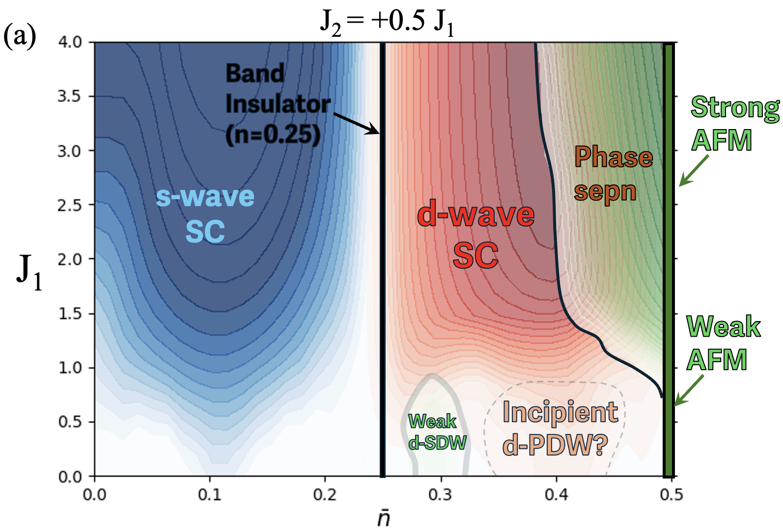
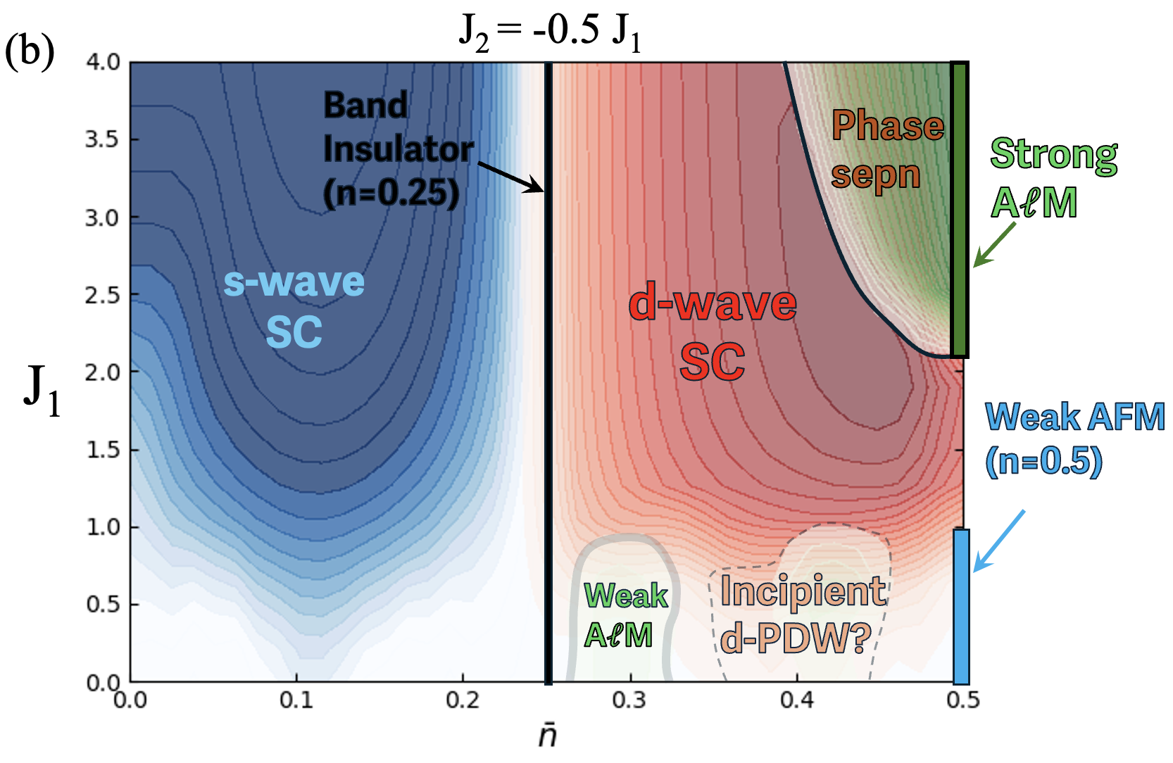
Figure 6: Mean field phase diagram of Hamiltonian in Eq. 1 with fixed $t_{1}=1$, $t_{2}=0.5t_{1}$, and inter-cell exchange coupling (a) $J_{2}=+0.5J_{1}$ and (b) $J_{2}=-0.5J_{1}$. In both models, we find regimes of $s$-wave and $d$-wave superconductors with color contours indicating qualitative variation of the pair order parameter. Over a small range of densities, quasi-1D van Hove singularity leads to weak uniform $A\ell M$ order for $J_{2}<0$, and a modulated $d$-spin density wave ($d$-SDW) order with $A\ell M$-type order within the unit cell for $J_{2}>0$. In addition, we find a small window at weak coupling labelled “incipient d-PDW” where small system size calculations seem to favor $(\pi,\pi)$ PDW with $d$-wave order over uniform $d$-wave SC, but the PDW order decreases with increasing system size. At half-filling and strong coupling, we find insulators with strong magnetic orders of AFM ($J_{2}>0$) or $A\ell M$ ($J_{2}<0$) type. The region marked ‘Phase sepn’ shows phase separation between $d$-wave SC and the insulating AFM or $A\ell M$ order. The magnetization and pairing patterns for these phases are shown in Fig.7, while the nature of phase separation is shown in Fig.9.

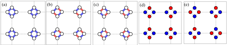
Figure 7: Order parameter patterns found in a quadrupled unit cell mean-field theory calculations. (a) uniform s-wave pairing with the same phase and strength of pairing on each intra-diamond bond. (b) uniform d-wave pairing with uniform strength but alternating phase of the pairing within the diamonds. (c) d-wave PDW with a d-wave pattern of pairing within the diamond, but now with a wave-vector of $M=(\pi,\pi)$. (d) Altermagnet with red marking spin-up and blue marking spin-down on site. The altermagnet ordering wave-vector is however simply $\Gamma$. (e) AFM with similar ordering within the diamond as the altermagnet, but with a wave-vector of $M$. The weak $d$-SDW is similar to AFM but has modulations at incommensurate wavevector driven by near nesting of Fermi surface segments.

(i) $s$-wave SC: In both cases, the low density $\bar{n}<0.25$ regime shows $s$-wave superconductivity. This is driven by the effective attractive Hubbard attraction induced by $J_{1}$ for the $s$-orbital as seen from Eq. 9. Dominant singlet pairing mainly occurs on bonds between sites within the unit-cell, with a weaker pairing on bonds connecting the diamond plaquettes. The largest pairing amplitude at any $J_{1}$ appears for densities $\bar{n}\approx 0.125$ which coincides with the 2D van Hove singularity in the density of states seen in Fig. 2. The structure of the pair amplitude on the unit cell, and the momentum dependent spectral gap at the chemical potential are shown in Fig. 7 (a).

(ii) AFM order: In both cases, we find a weak coupling instability at half-filling ($\bar{n}=0.5$) towards Néel AFM driven by nesting of the Fermi surfaces. We have confirmed this also within a random phase approximation (RPA) calculation discussed in the Appendix A.1. For the case $J_{2}>0$, this Stoner-type AFM order persists to strong coupling, much like in the one-band Hubbard model, leading to an AFM Mott insulator. For $J_{2}<0$, this Stoner AFM is absent as we increase $J_{2}$. Fig. 7 (e) depicts the magnetization in this AFM state.

(iii) Strong $A\ell M$ order: At half-filling, for $J_{2}<0$, going to strong coupling leads to $A\ell M$ order with a large ordered moment. This is an insulating $A\ell M$, driven by local moments coupled through $J_{1}>0$ and $J_{2}<0$, as can be qualitatively understood at the level of a classical spin model in a Mott insulator. Fig. 7 (d) shows the structure of the magnetization in this A$\ell$M state.

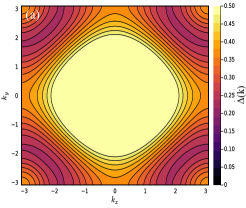
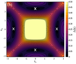
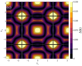
Figure 8: Illustrative plot of the gap in the Bogoliubov quasi-particle spectrum at (a) $\bar{n}=0.2$ with s-wave pairing amplitude $~{}0.1t_{1}$ (realized around $J_{1}\approx 1.5t_{1}$ in the mean-field theory) which is fully gapped, and (b) $\bar{n}=0.4$ also with d-wave pairing amplitude $~{}0.1t_{1}$ which shows Dirac nodes (marked with crosses ‘x’) along the $\Gamma\rightarrow X$, and $\Gamma\rightarrow Y$ paths in the Brillouin zone. (c) The corresponding case when a $(\pi,\pi)$ d-wave pairing with amplitude $~{}0.1t_{1}$ (this is exaggerated as compared to the mean-field results for illustrative purposes) is considered instead shows a gapless surface of quasiparticle excitations; for comparison with (b) we have plotted the spectrum in the original Brillouin zone.

(iv) Weak $A\ell M$ order: Remarkably, for $J_{2}<0$, we find a second window of weak $A\ell M$ order at weak coupling, for densities $0.26\lesssim\bar{n}\lesssim 0.3$, featuring a small ordered moment. This phase can be understood as being driven by the quasi-1D vHS seen in Fig. 2 corresponding to a low filling of the $X,Y$ bands. In this regime, it is well known that the divergent DOS leads to a strongly enhanced ferromagnetic Stoner susceptibility. The weak $A\ell M$ phase then results from the effective AFM Hund’s coupling seen in Eq. 10 between weakly ferromagnetic X and Y chains in the projected two-orbital model. The weak $A\ell M$ state has the same symmetry as the strong coupling $A\ell M$, except for a highly reduced moment. For $J_{2}>0$, we find a weak SDW ordering in the same density regime; however, the ordering wave-vector is $\mathbf{Q}\approx M/2$, with a $d$-type ordering within the unit cell (similar to the $A\ell M$). This ordering wavevector corresponds to the approximate nesting of the Fermi surface at these densities; this instability is further bolstered by interactions (see Appendix A.1 for results from RPA calculation).

(v) Uniform $d$-wave SC: Both models, with weak $J_{2}<0$ and $J_{2}>0$, show large regimes of uniform singlet $d$-wave superconductivity for $0.25<\bar{n}<0.5$. This is primarily driven by the formation of singlet Cooper pairs on bonds with the unit cell plaquettes, driven by AFM $J_{1}>0$, which can then delocalize across the lattice. In the projected model, this phase can be simply viewed as the local AFM Hund’s coupling leading to a nonzero on-site order parameter $\langle X^{\dagger}Y^{\dagger}\rangle$. Since $C_{4}$ rotation leads to $X\to Y$ and $Y\to-X$, this local order parameter changes sign in accordance with $d$-wave symmetry. In several instances, we have found that real space solutions of the mean field equations starting from random initial conditions result in $d$-wave droplets which are not fully phase-locked across the lattice, suggestive of a not-very-strong superfluid stiffness; in future work, we will address the superfluid stiffness in these regimes. However, in all these cases, we have checked that the uniform $d$-wave solution has a slightly lower energy than these phase-random $d$-wave droplet solutions. Fig. 7(b) and  8(b) show the pair amplitude in real space, and the momentum dependent spectral gap at the chemical potential.

(vi) $d$-wave PDW order: Interestingly, for $J_{1}\lesssim 1.0$ and for $0.38\lesssim n\lesssim 0.48$, we find regimes of $(\pi,\pi)$ $d$-wave PDW order in our inhomogeneous mean field theory on system sizes upto $6\times 6$ unit cells. In this $d$-PDW, electrons form singlet $d$-wave pairs within the unit cell but the pairing amplitude changes sign in the adjacent unit cell. Fig. 7(c) shows the structure of the pair amplitude on the unit cell, and Fig. 8(c) shows the resulting momentum dependent spectral gap in the full Brillouin zone. The RPA pairing susceptibility in the normal state shows significant peaks at $(0,0)$ and $(\pi,\pi)$ (see Appendix A.2); however, the most divergent low temperature susceptibility is at $(0,0)$, suggesting that this finite size $d$-wave PDW order should disappear with increasing system size as we have confirmed using momentum space mean field theory. However, the fact that the PDW state is favored on small system sizes suggests that slightly tuning the interactions, perhaps by including further neighbor interactions could favor this as the true ground state, as suggested in recent work on other models [64].

(vii) Coexistence / Phase separation: Finally, in the strong coupling regime and for small doping away from half-filling, we find a regime where $d$-wave superconductivity and AFM or $A\ell M$ coexist in uniform mean field theory. In this pairing state, the $A\ell M$ order mixes the real space singlet $d$-wave and triplet $s$-wave pairing with $S_{z}=0$ on the diamond unit cell, which is allowed by the presence of multiple orbitals, leading to a state which is odd under ${\mathcal{C}}_{4}{\mathcal{T}}$. Allowing for a spatially inhomogeneous state, these coexisting orders phase separate, with the magnetically ordered regimes having density $\bar{n}\approx 0.5$ and forming Mott insulator droplets while the lower density regimes have $d$-wave pairing. In this regime, a uniform ansatz favors coexistence of AFM / $A\ell M$ order with superconductivity. This coexistence leads to mixed singlet-triplet pairing within the unit cell; such $A\ell M$-induced triplet pairing has been explored in recent work discussing $A\ell M$ fluctuation induced pairing [29, 30, 31, 32]. Incorporating longer-range repulsion between doped charges could lead to organization of these phase separated regions into stripe or checkerboard states as has also been found in models for the cuprate superconductors. Fig. 9 shows the typical structure of the density, magnetization, and pairing amplitude in such a phase separated state.

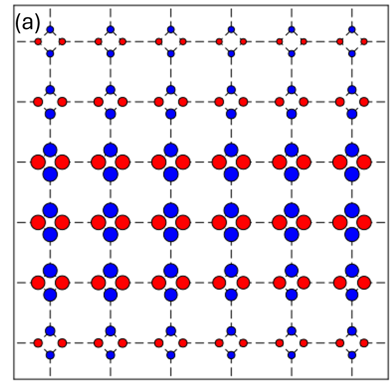
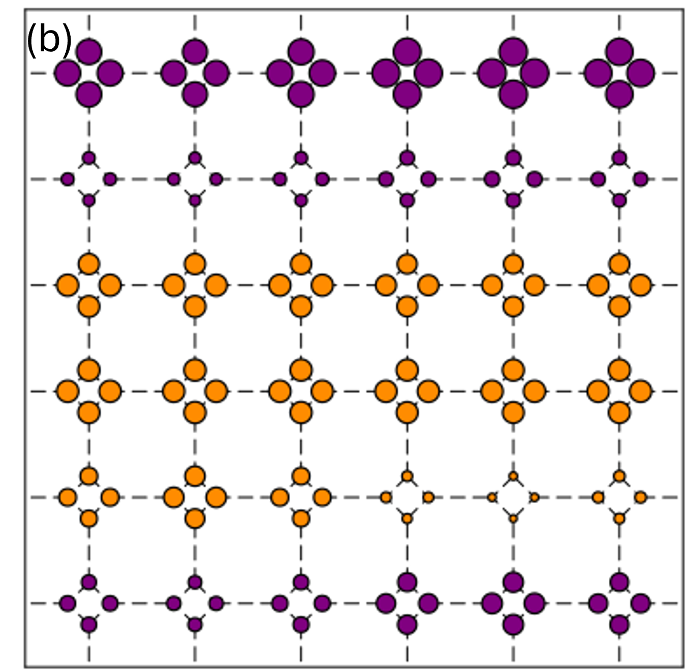
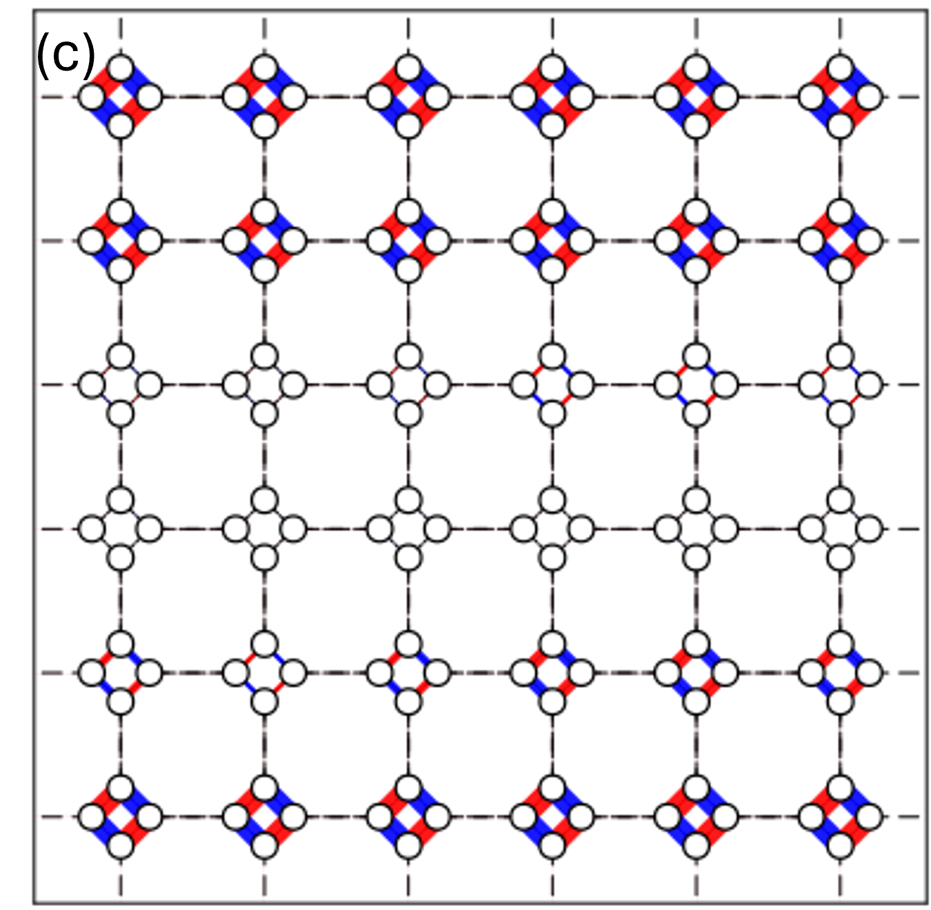
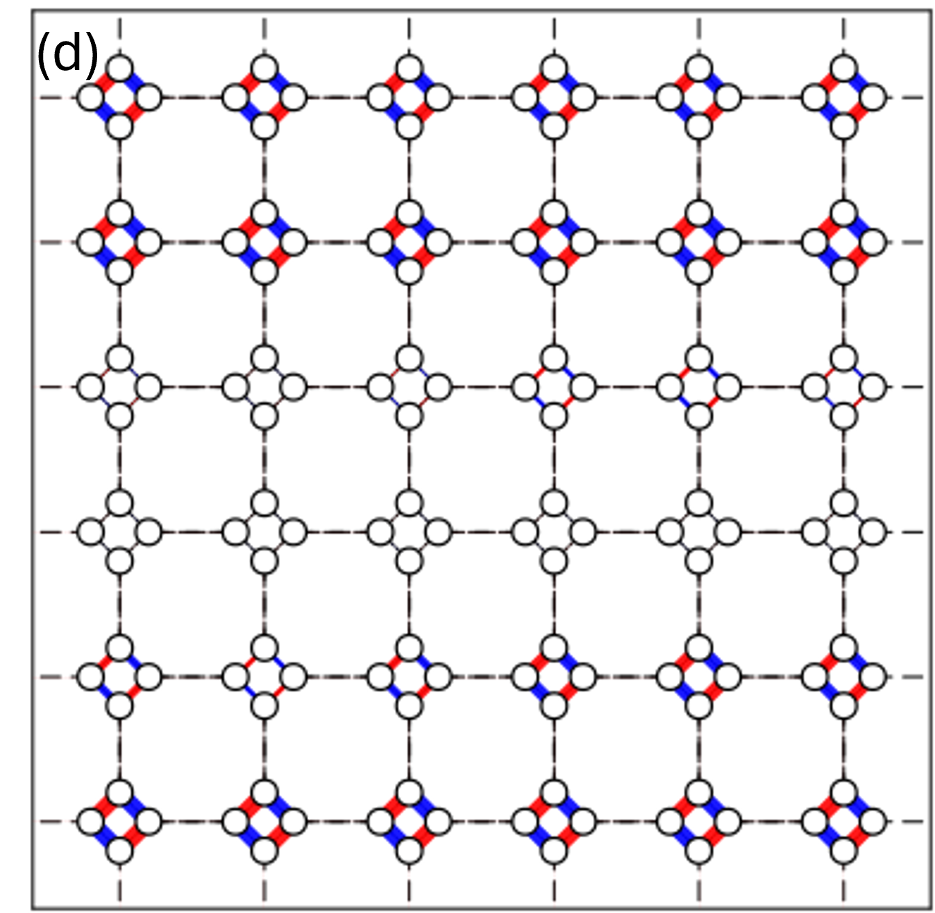
Figure 9: Example of converged real space mean field solution at $\bar{n}=0.46$, $J_{2}=-0.5J_{1}$, and $J_{1}=3.6$, showing phase separated state. (a) Inhomogeneous magnetic order of $A\ell M$ type with strong and weak $A\ell M$ regions. The weak $A\ell M$ order is induced by proximity to the strong $A\ell M$ region. (b) Density modulations which track the $A\ell M$ modulations with strong $A\ell M$ order corresponding to density $\bar{n}\approx 0.5$ and weak $A\ell M$ regions having density $\bar{n}<0.46$. (c) spatially inhomogeneous singlet pairing, and (d) spatially inhomogeneous triplet pairing. The mixture of $d$-wave singlet and triplet pairing in regions of low $A\ell M$ order is also driven by proximity to the $A\ell M$ domain, similar in spirit to the work by Brekke, et al [29].

IV Summary and discussion

Motivated by exploring $t$-$J$ models which capture $A\ell M$ order and to study the possible effects of doping and pressure-tuning of bandwidth, we have discussed a mean field theory of a minimal model on the square-octagon lattice. This is shown to have a phase diagram which includes multiple types of $A\ell M$ order - a strongly ordered phase with large moment at strong coupling and a weakly ordered phase driven by quasi-1D van Hove singularities. The latter suggests a possible alternative design route to realizing weak $A\ell M$ order in materials. In addition, our phase diagram features multiple types of superconducting orders including $s$-wave, $d$-wave, and possible $d$-wave PDW order. For $J_{2}>0$ coupling between unit cells, this leads to locally $A\ell M$-type configuration which is modulated at an incommensurate wavevector $Q$ which we have dubbed $d$-SDW. We discussed the spatial structure of the various broken symmetry states and presented aspects of the spectral gap features in these phases. We are currently exploring if incorporating additional interactions in this model could stabilize stable PDW order. It would be interesting to also explore if such a rich set of orders are generic in other $A\ell M$ models with orbital and spin order which have been explored in recent work [69, 70] which would provide further motivation for experimentalists to search for superconductivity in doped or pressurized $A\ell M$ materials. Finally, incorporating weak spin-orbit coupling effects in these $tJ$ models might be a route to interesting topological superconducting phases and would be a useful direction for future research.

Appendix A Susceptibilities

To get an idea of possible instabilities, one can calculate the susceptibility of these multi-orbital or multi-sublattice model towards them. The formulation is a bit more involved but essentially the same as the simple single-band case. Furthermore, to leading order, one can also look at the effects of the interaction under RPA type approximation. To begin by looking at bare susceptibilities, let us define the generalized Hubbard Stratonovich (HS) fields corresponding to our orderings as

• Magnetic order : Define the local HS fields as $\phi_{\mathbf{r},i}^{a}(\tau)=(1/2)f^{\dagger}_{\mathbf{r},i,\alpha}(\tau)\sigma^{a}_{\alpha\beta}f_{\mathbf{r},i,\beta}(\tau)$, where $\mathbf{r}$ refers to the unit-cell position, $i$ refers to every degree of freedom other than spin (such as sublattice or orbital), $a=x,y,z$ refers to the spin-ordering direction, and $\alpha,\beta$ refers to the fermion spin. In momentum space the corresponding vertex looks like

  $$\phi_{\mathbf{Q},i}^{a}(i\Omega)=\sigma^{a}_{\alpha\beta}\int\frac{d^{2}k}{(2\pi)^{2}}\int\frac{d\omega}{(2\pi)}f^{\dagger}_{\mathbf{Q}+\mathbf{k},i,\alpha}(i\Omega+i\omega)f_{\mathbf{k},i,\beta}(i\omega)\,,$$ (11)

  where $\mathbf{Q}$ is the exchange momentum and $\Omega$ is the exchange energy.

• Pairing order : Now pairing is more complicated since one can have non-local pairing as well. To that end, a generalized pairing HS field will look like $\Delta_{\mathbf{r+\delta/2}}^{a,ij}(\tau)=(1/2)f^{\dagger}_{\mathbf{r},i,\alpha}(\tau)\sigma^{a}_{\alpha\beta}f^{\dagger}_{\mathbf{r+\delta},j,\beta}(\tau)$ corresponding to a non-local pairing when $\delta\neq 0$. Such HS fields generically live on the bonds of the lattice as opposed to the magnetic ordering field living on-site. Again, in Fourier space, the vertex (which is now momentum dependent) looks like

  $$\Delta_{\mathbf{Q},ij}^{a}(\bm{\delta};i\Omega)=\sigma^{a}_{\alpha\beta}\int\frac{d^{2}k}{(2\pi)^{2}}\int\frac{d\omega}{(2\pi)}f^{\dagger}_{-\mathbf{k}+\mathbf{Q}/2,i,\alpha}(-i\omega+i\Omega/2)f^{\dagger}_{\mathbf{k}+\mathbf{Q}/2,j,\beta}(i\omega+i\Omega/2)e^{i\bm{\delta}\dotproduct\mathbf{k}}\,,$$ (12)

  where $\mathbf{Q}$ is the center of mass momentum and $\Omega$ is the center of mass energy.

Using these HS fields, we can calculate the bare susceptibility of the model as shown in the subsequent sections. To get ordering tendencies of the model, we have to diagonalize the zero-energy response matrix at all momenta. The eigenvector with the largest eigenvalue corresponds to possible orderings with the ordering vector being the momentum at which this maximum eigenvalue occurs. One can repeat this exercise after performing RPA, which can affect possible orderings in the model as interaction strength is slowly increased. Encountering a diverging eigenvalue of the response corresponds to a phase transition into a symmetry broken state, which should match qualitatively with mean-field results. Alternatively, one can also tune the temperature at strong coupling regime to extract information about phases beyond the first instability encountered at zero temperature when tuning the interaction.

A.1 Magnetic channel

The bare susceptibility, $\chi_{0,ij}^{ab}(\mathbf{Q},i\Omega)=\expectationvalue{\phi_{\mathbf{Q},i}^{a}(i\Omega)\phi_{\mathbf{Q},j}^{b,\dagger}(i\Omega)}$ is equivalent to the usual spin-response function. Diagrammatically, it corresponds to a generalized bubble diagram. For spin-rotation symmetric systems, the connected piece of the diagram looks like

$$\chi_{0,ij}^{ab}(\mathbf{Q},i\Omega)=-\frac{\delta^{ab}}{4}\int\frac{d^{2}k}{(2\pi)^{2}}\int\frac{d\omega}{(2\pi)}G_{ij}(\mathbf{Q}+\mathbf{k},i\Omega+i\omega)G_{ji}(\mathbf{k},i\omega)\,,$$ (13)

where $G_{ij}^{\alpha\beta}(\mathbf{k},i\omega)=\delta^{\alpha\beta}G_{ij}(\mathbf{k},i\omega)=\expectationvalue{f^{\dagger}_{i,\alpha}(\mathbf{k},i\omega)f_{j,\beta}(\mathbf{k},i\omega)}$ are the bare Green’s functions calculated in mean-field theory. In terms of the quasi-particle dispersion, $\epsilon_{n}(\mathbf{k})$, and their corresponding wavefunctions $U_{ij}(\mathbf{k})$, these Green’s functions can be expressed as

$$G_{ij}(\mathbf{k},i\omega)=\sum_{n}U_{jn}(\mathbf{k})\frac{1}{i\omega-\epsilon_{n}(\mathbf{k})+\mu}U^{\dagger}_{ni}(\mathbf{k})\,.$$ (14)

Substituting this expression back into (15), performing the Matsubara sum by hand, and analytically continuing the resulting expression $i\Omega\rightarrow\Omega+i\eta$, we get

$$\chi_{0,ij}^{ab}(\mathbf{Q},i\Omega)=\frac{\delta^{ab}}{4}\sum_{n,m}\int\frac{d^{2}k}{(2\pi)^{2}}U_{jn}(\mathbf{Q}+\mathbf{k})U_{ni}^{\dagger}(\mathbf{Q}+\mathbf{k})U_{im}(\mathbf{k})U_{mj}^{\dagger}(\mathbf{k})\frac{n_{F}(\epsilon_{n}(\mathbf{Q}+\mathbf{k})-\mu)-n_{F}(\epsilon_{m}(\mathbf{k})-\mu)}{\Omega+i\eta-(\epsilon_{n}(\mathbf{k}+\mathbf{Q})-\epsilon_{m}(\mathbf{k}))}\,,$$ (15)

where $n_{F}$ is the Fermi distribution function.

To perform RPA, let us focus on analyzing Heisenberg type interactions and decompose it in terms of the magnetic HS fields. We have a generalized Heisenberg type interaction on a lattice as

$${\mathcal{H}}_{int}=\frac{1}{4}\sum_{\bm{\delta}}\sum_{\mathbf{r},\tau}J_{ij}(\bm{\delta})f^{\dagger}_{\mathbf{r},i,\alpha}(\tau)\sigma^{a}_{\alpha\beta}f_{\mathbf{r},i,\beta}(\tau)f^{\dagger}_{\mathbf{r}+\bm{\delta},j,\mu}(\tau)\sigma^{a}_{\mu\nu}f_{\mathbf{r}+\bm{\delta},j,\nu}(\tau)\,.$$ (16)

Using the definition of the magnetic HS fields, we immediately see that

$$\begin{split}{\mathcal{H}}_{int}&=\sum_{\bm{\delta}}\sum_{\mathbf{r},\tau}J_{ij}(\bm{\delta})\phi_{\mathbf{r},i}^{a}(\tau)\phi^{a,\dagger}_{\mathbf{r}+\bm{\delta},j}(\tau)\\ &=\sum_{\mathbf{Q},\Omega}\phi_{\mathbf{Q},i}^{a}(\Omega)\left[\delta^{ab}\sum_{\bm{\delta}}J_{ij}(\bm{\delta})e^{-i\mathbf{Q}\dotproduct\bm{\delta}}\right]\phi^{b,\dagger}_{\mathbf{Q},j}(\Omega)\,.\end{split}$$ (17)

Hence, under RPA, the susceptibility will have the form

$$\chi_{ij}^{ab}(\mathbf{Q},\Omega)=\left[\left(\mathds{1}-\chi_{0}(\mathbf{Q},\Omega)\dotproduct\tilde{J}(\mathbf{Q})\right)^{-1}\dotproduct\chi_{0}(\mathbf{Q},\Omega)\right]_{ij}^{ab}\,,$$ (18)

where the effective interaction matrix is $\tilde{J}_{ij}^{ab}(\mathbf{Q})=\delta^{ab}\sum_{\bm{\delta}}J_{ij}(\bm{\delta})e^{-i\mathbf{Q}\dotproduct\bm{\delta}}$, and $\dotproduct$ denotes matrix multiplication in the spin-direction index $a$ and sublattice/orbital index $i$ .

For our model, with $J_{2}/J_{1}<0$ shown in Fig.11, we find that at exactly half-filling $\bar{n}=0.5$, there is an instability towards AFM order which can be seen by the response peaking near the $M=(\pi,\pi)$ point in the Brillouin zone. However, at every other generic filling, the system prefers $A\ell M$ ordering, peaked at the $\Gamma$ point. Whereas, for $J_{2}/J_{1}>0$ as shown in Fig.12, the instability towards AFM at half-filling is still there, but the instability at lower filling near the van-Hove singularities is now with $Q=M/2$. This comes up due to Fermi-surface nesting around that filling, as can be seen even in the bare susceptibilities in Fig.10.

Figure 10: The bare magnetic susceptibilities at zero-energy at a fixed low temperature of $T=0.1t_{1}$ plotted along a high-symmetry path in the Brillouin zone, at two different fillings. The labels describe the eigenvectors of the susceptibility matrix such that $s-like$ corresponds to all spins pointing parallel to each other in the unit cell, $d-like$ corresponds to the spins alternating within the unit cell and so on. (a) At half-filling,$\bar{n}=0.5$, where we find the ordering at $Q=M$ with a $d-like$ eigenvector. This just corresponds to a usual AFM ordering. (b) At some generic filling, $\bar{n}=0.3$, we find more complicated momentum-dependent behaviour which is peaked near $Q=\Gamma$, again with the $d$ type eigenvector.

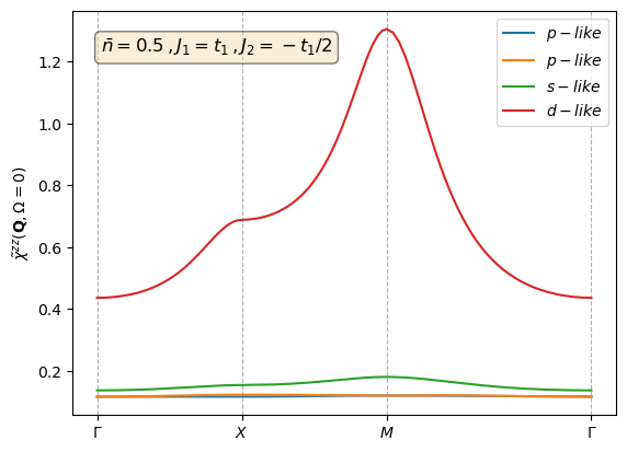
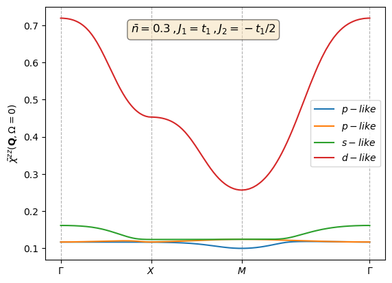
Figure 11: The magnetic susceptibilities at zero-energy at a fixed low temperature of $T=0.1t_{1}$ after performing RPA at $J_{1}=t_{1},J_{2}=-0.5t_{1}$,plotted along a high-symmetry path in the Brillouin zone, at two different fillings. The labels are the same as in Fig.10 (a) At half-filling,$\bar{n}=0.5$, the ordering at $Q=M$ with a $d-like$ eigenvector corresponding to the usual AFM ordering. (b) At some generic filling, $\bar{n}=0.3$, the RPA susceptibility is peaked at $Q=\Gamma$, again with the $d$ type eigenvector. This corresponds to a $A\ell M$ type ordering.

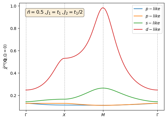
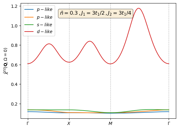
Figure 12: The magnetic susceptibilities with $J_{2}/J_{1}>0$ at zero-energy at a fixed low temperature of $T=0.1t_{1}$ after performing RPA, plotted along a high-symmetry path in the Brillouin zone, at two different fillings. The labels are the same as in Fig.10 (a) At half-filling,$\bar{n}=0.5$, the ordering at $Q=M$ with a $d-like$ eigenvector corresponding to the usual AFM ordering. (b) At $\bar{n}=0.3$ close to the Van-hove singularities, the ordering is at $Q~{}M/2$ with a d-type eigenvector.

A.2 Pairing channel

Let us look at the bare pairing susceptibility by repeating the steps as in the magnetic case (with a lot more indices to keep track of!). We want to calculate $\Gamma_{0,ijkl}^{ab}(\bm{\delta}_{1},\bm{\delta}_{2};\mathbf{Q},i\Omega)=\expectationvalue{\Delta_{\mathbf{Q},ij}^{a}(\bm{\delta}_{1};i\Omega)\Delta_{\mathbf{Q},kl}^{b,\dagger}(\bm{\delta}_{2},i\Omega)}$. Working this bubble out in all its gory details gives us

$$\begin{split}\Gamma_{0,ijkl}^{ab}(\bm{\delta}_{1},\bm{\delta}_{2};\mathbf{Q},i\Omega)=\frac{1}{4}\sigma^{a}_{\alpha\beta}\sigma^{b}_{\mu\nu}\int\frac{d^{2}k}{(2\pi)^{2}}\int\frac{d\omega}{(2\pi)}\bigg{\{}&e^{i\mathbf{k}\dotproduct(\bm{\delta}_{1}-\bm{\delta}_{2})}G_{ik}^{\alpha\delta}(-\mathbf{k}+\mathbf{Q}/2,-i\omega+i\Omega/2)G_{jl}^{\beta\gamma}(\mathbf{k}+\mathbf{Q}/2,i\omega+i\Omega/2)\\ -&e^{i\mathbf{k}\dotproduct(\bm{\delta}_{1}+\bm{\delta}_{2})}G_{il}^{\alpha\mu}(-\mathbf{k}+\mathbf{Q}/2,-i\omega+i\Omega/2)G_{jk}^{\beta\nu}(\mathbf{k}+\mathbf{Q}/2,i\omega+i\Omega/2)\bigg{\}}\,.\end{split}$$ (19)

We can simplify the above expression when we use spin-rotation symmetry which tells us that the pairing response can be categorized into singlet and triplet pairings. Defining a shorthand for one of the two contributions to the integral as

$${\mathcal{I}}_{ijkl}(\bm{\delta};\mathbf{Q},i\Omega)\equiv\int\frac{d^{2}k}{(2\pi)^{2}}\int\frac{d\omega}{(2\pi)}e^{i\mathbf{k}\dotproduct\bm{\delta}}G_{ik}(-\mathbf{k}+\mathbf{Q}/2,-i\omega+i\Omega/2)G_{jl}(\mathbf{k}+\mathbf{Q}/2,i\omega+i\Omega/2)\,,$$ (20)

we get that

$$\Gamma_{0,ijkl}^{ab}(\bm{\delta}_{1},\bm{\delta}_{2};\mathbf{Q},i\Omega)=\begin{cases}\frac{1}{2}{\mathcal{I}}_{ijkl}(\bm{\delta}_{1}-\bm{\delta}_{2};\mathbf{Q},i\Omega)-\frac{1}{2}{\mathcal{I}}_{ijlk}(\bm{\delta}_{1}+\bm{\delta}_{2};\mathbf{Q},i\Omega)\,,\>\>\>a=b\in\{0,x,z\}:\text{ triplet}\,,\\ \frac{1}{2}{\mathcal{I}}_{ijkl}(\bm{\delta}_{1}-\bm{\delta}_{2};\mathbf{Q},i\Omega)+\frac{1}{2}{\mathcal{I}}_{ijlk}(\bm{\delta}_{1}+\bm{\delta}_{2};\mathbf{Q},i\Omega)\,,\>\>\>a=b\in\{y\}:\text{ singlet}\,,\\ 0\,,\>\>\>a\neq b\,,\end{cases}$$ (21)

where $\sigma^{0}=\mathds{1}_{2\times 2}$, the identity matrix. Focusing on ${\mathcal{I}}_{ijkl}$, we can repeat the steps as before i.e. write everything using the band dispersion and wavefunctions, performing the Matsubara sum by hand, and analytically continuing the resultant expression. We end up with

$$\begin{split}{\mathcal{I}}_{ijkl}(\bm{\delta};\mathbf{Q},\Omega)=\sum_{n,m}\int\frac{d^{2}k}{(2\pi)^{2}}&U_{kn}(-\mathbf{k}+\mathbf{Q}/2)U^{\dagger}_{ni}(-\mathbf{k}+\mathbf{Q}/2)U_{lm}(\mathbf{k}+\mathbf{Q}/2)U^{\dagger}_{mj}(\mathbf{k}+\mathbf{Q}/2)\\ \times&\left(\frac{n_{F}(\epsilon_{n}(-\mathbf{k}+\mathbf{Q}/2)-\mu)+n_{F}(\epsilon_{m}(\mathbf{k}+\mathbf{Q}/2)-\mu)-1}{\Omega+i\eta-\epsilon_{n}(-\mathbf{k}+\mathbf{Q}/2)-\epsilon_{m}(\mathbf{k}+\mathbf{Q}/2)+2\mu}\right)\,.\end{split}$$ (22)

Now, for RPA in this channel, we will have to redo the decomposition of the interaction in terms of the pairing HS fields. We again start with (16) and rearrange the terms as

$${\mathcal{H}}_{int}=\frac{1}{4}\sigma^{a}_{\alpha\beta}\sigma^{a}_{\mu\nu}\sum_{\bm{\delta}}\sum_{\mathbf{r},\tau}J_{ij}(\bm{\delta})f^{\dagger}_{\mathbf{r},i,\alpha}(\tau)f^{\dagger}_{\mathbf{r}+\bm{\delta},j,\mu}(\tau)f_{\mathbf{r}+\bm{\delta},j,\nu}(\tau)f_{\mathbf{r},i,\beta}(\tau)\,.$$ (23)

Figure 13: The normal state RPA singlet pairing susceptibility with $t_{1}=1$, $t_{2}=0.5t_{1}$, $J_{1}=0.5t_{1}$ and $J_{2}=-0.5J_{1}$ at $\Omega=0$ and a fixed low temperature of $T=0.13t_{1}$, plotted on the Brillouin zone for the reduced two-orbital model. The largest eigenvalue comes from the $X-Y$ singlet pairing on-site which corresponds to a $d$-wave pairing in the original model.

We see that we cannot simply substitute the form of our pairing HS fields since the spin-indices are not as we want them in (23). However, since the Heisenberg interaction is spin-rotation symmetric, we can again decompose it in terms of singlet and triplets. It turns out that the interaction then looks like

$$\begin{split}{\mathcal{H}}_{int}&=\frac{1}{4}\sum_{\bm{\delta}}\sum_{\mathbf{r},\tau}J_{ij}^{ab}(\bm{\delta})\left(f^{\dagger}_{\mathbf{r},i,\alpha}(\tau)\sigma^{a}_{\alpha\mu}f^{\dagger}_{\mathbf{r}+\bm{\delta},j,\mu}(\tau)\right)\left(f_{\mathbf{r}+\bm{\delta},j,\nu}(\tau)\sigma^{b}_{\nu\beta}f_{\mathbf{r},i,\beta}(\tau)\right)\\ &=\sum_{\bm{\delta}}\sum_{\mathbf{r},\tau}J_{ij}^{ab}(\bm{\delta})\Delta_{\mathbf{r}+\bm{\delta}/2}^{a,ij}(\tau)\Delta_{\mathbf{r}+\bm{\delta}/2}^{b,ij,\dagger}(\tau)\,,\\ &=\sum_{\mathbf{Q},\Omega}\Delta_{\mathbf{Q},ij}^{a}(\bm{\delta}_{1};\Omega)\left[\delta^{(ij),(kl)}\delta_{\bm{\delta}_{1},\bm{\delta}_{2}}\sum_{\bm{\delta}}J_{ij}^{ab}(\bm{\delta}_{1})\right]\Delta_{\mathbf{Q},kl}^{b,\dagger}(\bm{\delta}_{2};\Omega)\,,\end{split}$$ (24)

where the interaction in the singlet-triplet pairing basis looks like

$$J_{ij}^{ab}(\bm{\delta})=\begin{cases}\frac{1}{2}J_{ij}(\bm{\delta})\,,\>\>\>a=b\in\{0,x,z\}:\text{ triplet}\,,\\ -\frac{3}{2}J_{ij}(\bm{\delta})\,,\>\>\>a=b\in\{y\}:\text{ singlet}\,,\\ 0\,,\>\>\>a\neq b\,.\end{cases}$$ (25)

Note that the interaction is completely momentum independent in the center of mass basis, and diagonal in the pairing HS fields! The total RPA susceptibility takes on a similar form as (18) as

$$\Gamma_{ijkl}^{ab}(\bm{\delta}_{1},\bm{\delta}_{2};\mathbf{Q},i\Omega)=\left[\left(\mathds{1}-\Gamma_{0}(\mathbf{Q},i\Omega)\dotproduct{\mathcal{J}}(\mathbf{Q})\right)^{-1}\dotproduct\Gamma_{0}(\mathbf{Q},i\Omega)\right]_{ijkl}^{ab}(\bm{\delta}_{1},\bm{\delta}_{2})\,,$$ (26)

where ${\mathcal{J}}_{ij,kl}^{ab;\bm{\delta}_{1}\bm{\delta}_{2}}(\mathbf{Q})=\delta^{(ij),(kl)}\delta_{\bm{\delta}_{1},\bm{\delta}_{2}}\sum_{\bm{\delta}}J_{ij}^{ab}(\bm{\delta}_{1})$, and $\dotproduct$ now denotes matrix multiplication in all possible index degree of freedom including spin $a$, bond displacement $\bm{\delta}$, and pairing orbital/sublattices $ij$.

For simplicity, we chose to use the reduced two-orbital model instead of the full square-octagon model, and focus on singlet pairing susceptibility. The pairing HS fields we choose to work with are the ones which can be generated through our interaction, namely $X-Y$ pairing on site $\Delta_{\mathbf{Q},XY}^{y}(\mathbf{0};0)$, $X-X$ pairing along the $x$-bonds $\Delta_{\mathbf{Q},XX}^{y}(\hat{x};0)$, and $Y-Y$ pairing along the $y$-bonds $\Delta_{\mathbf{Q},YY}^{y}(\hat{y};0)$. Note that since $\Delta_{\mathbf{Q},ij}^{a}(\bm{\delta};i\Omega)=\Delta_{\mathbf{Q},ji}^{a}(-\bm{\delta};i\Omega)$, we do not need to track $\bm{\delta}=-\hat{x}$ and $\bm{\delta}=-\hat{y}$ separately.

We find that the largest eigenvalue comes from the $X-Y$ pairing on-site as shown in Fig.13. Upon RPA, above the critical temperature $T_{C}$, we find that the peak in the center of mass momentum is at the Gamma point $\mathbf{Q}=\Gamma$. However, we also note that there are secondary peaks at the $M$ points as well, which explains the strong competition between a $(\pi,\pi)$ PDW versus a simple $d$-wave pairing. In future works, one can imagine adding additional interactions which will further enhance the peak at the $M$ points. Lastly, since its the $J_{1}$ interaction which enhances these responses, changing the sign of $J_{2}$ from being ferromagnetic to anti-ferromagnetic shows minor changes in the susceptibility in the cases when $|J_{2}|<<|J_{1}|$.