Exclusive Bremsstrahlung of One and Two Photons in Proton-Proton Collisions ††thanks: Presented by A. Szczurek at XXX Cracow EPIPHANY Conference on Precision Physics at High Energy Colliders, Kraków, Poland, January 8-12, 2024.
Abstract
We discuss the diffractive bremsstrahlung of a single photon in the reaction at LHC energies and at forward photon rapidities. We compare the results for our standard approach, based on QFT and the tensor-Pomeron model, with two versions of soft-photon approximations, SPA1 and SPA2, where the radiative amplitudes contain only the leading terms proportional to (the inverse of the photon energy). SPA1, which does not have the correct energy-momentum relations, performs surprisingly well in the kinematic range considered, namely at very forward photon rapidities and , the relative energy loss of the protons, corresponding to small values of the photon transverse momentum. Azimuthal correlations between outgoing particles are presented. We discuss also the role of the background for single photon production. We discuss also the possibility of a measurement of the reaction. Our predictions can be verified by ATLAS-LHCf combined experiments.
1 Introduction
In this contribution we will be concerned with exclusive diffractive photon(s) bremsstrahlung in proton-proton collisions at high energies. The presentation is based on [2, 1] where all details and many more results can be found.
The forward photon production (inclusive) cross-section in proton-proton collisions was measured with the RHICf detector [6] at centre-of-mass energy GeV and with the LHCf detector at and 13 TeV [7]. The LHCf experiment is designed to measure the production cross section of neutral particles in the pseudorapidity region , up to zero-degree. Several joint analyses with the ATLAS-LHCf detectors are planned; see [8] and references therein. In contrast, the exclusive reaction has not yet been identified experimentally. Some feasibility studies for the measurement of the exclusive bremsstrahlung cross-sections were performed for RHIC energies [3] and for LHC energies using the ATLAS forward detectors [4, 5].
The theoretical methods which we use in our analysis were developed by us in [9, 2]. In [9] we discussed the soft-photon radiation in pion-pion scattering. There we compared our standard (called also “exact”) model results for diffractive photon-bremsstrahlung to various soft-photon approximations (SPAs) based on the soft-photon theorems. In [2] we extended these considerations to the reaction at TeV. In contrast to the analysis of this reaction previously discussed by two of us [10] in our recent works we use the tensor-Pomeron model developed in [11, 12]. The tensor-Pomeron model was successfully applied to many hadronic reactions, in particular to central exclusive diffractive production processes; see e.g. [14]. From [11, 12] we know the form of the effective Pomeron propagator and the Pomeron-proton-proton vertex function. We have shown in [15] that the photon-Pomeron fusion mechanism does not play an important role at very forward photon rapidities, which is what we are most interested in. In our analysis of photon-bremsstrahlung processes [9, 2] we respect the general QFT structure of the radiative amplitudes.
It is worth noting that for , in the region where soft-photon theorems discussed in[16] should be applicable, our bremsstrahlung distributions presented below and in [2, 1] are an exact result of QCD plus lowest order electromagnetism.
The theoretical methods which we developed for the exclusive diffractive bremsstrahlung of soft photons can be also used for the production of “dark photons”. For some interesting scenarios in this context, we refer the reader to Refs. [17, 18, 19]. Searching for a signal of light, weakly-interacting dark photons and many other long-lived particles of new physics, in the very forward region, is the main task of the FASER detector at the LHC [20].
2 Sketch of the formalism
2.1
We consider the reaction
| (1) |
at high energies and small momentum transfers. The momenta are indicated in brackets, the helicities of the protons are denoted by , and is the polarization vector of the photon. The kinematic variables are
| (2) |
The rapidity of the photon is then
| (3) |
where is the polar angle of , . The proton relative energy-loss parameters can be expressed by the kinematical variables of the photon,
| (4) |
() ()
() ()
()
The cross section for the photon yield can be calculated as follows
| (5) |
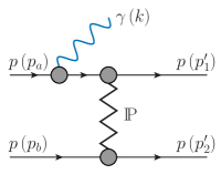
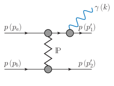
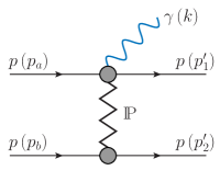
see Eqs. (2.33)–(2.35) of [2]. Above , is the radiative amplitude. In the following, we consider only the leading Pomeron-exchange contribution within the tensor-Pomeron approach [11, 12]. Our diffractive photon-bremsstrahlung amplitude includes 6 diagrams (see Fig. 1) ; see (2.62) and (B3) of [2]. The amplitudes corresponding to photon emission from the external protons are determined by the off-shell elastic scattering amplitude. The contact terms are needed in order to satisfy gauge-invariance constraints. With the off-shell elastic scattering amplitude , the standard proton propagator , and the vertex function, we get the following radiative amplitudes:
| (6) | |||||
In our tensor-product notation, the first factors will always refer to the - line, and the second refer to the - line. Using the Ward-Takahashi identity
| (7) |
and imposing the gauge-invariance condition we obtain
| (8) |
In a similar way we proceed with the amplitudes , , and . For details how to calculate above results we refer the reader to Sec. II C and Appendix B of [2].
We compare our standard results to two soft-photon approximations, SPA1 and SPA2, where we keep only the pole terms . In SPA1, the radiative amplitude has the form
| (9) |
where is the amplitude for on-shell -scattering. In the SPA1, the photon momentum was, on purpose, omitted in the energy-momentum conserving function in the evaluation of the cross section.
2.2
Here we consider two-photon bremsstrahlung in the reaction (see Fig. 2)
| (11) |
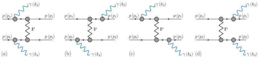
For the calculation of amplitude (11) we use SPA1:
| (12) | |||||
In this case, we shall require that one photon is emitted at forward and one at backward rapidities, and , respectively, and that , where we define
| (13) |
3 Results
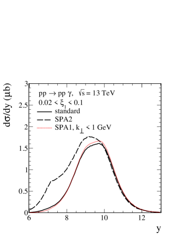
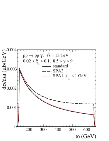
In Fig. 1 we show the distributions for our standard approach for the reaction together with the results obtained via SPA1 (9) and SPA2 (10). Recall that in both SPAs we keep only the pole terms in the radiative amplitudes. Bremsstrahlung photons are emitted predominantly in very forward-rapidity region and with small values of photon transverse momentum . Photons can be measured by the LHCf detectors, in the region , and the protons by the ATLAS forward proton spectrometers (AFP). Due to the limitation the energy of the photons is limited to . The SPA1 result performs surprisingly well in the kinematic range considered. For the SPA2, the deviations from our exact (standard) result increase rapidly with growing and . There is an important the interference between the leading term and the non-leading terms occurring in the radiative amplitudes. For more details on the size of various contributions we refer to the discussions in [2] and Fig. 17 therein.
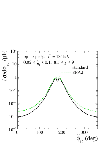
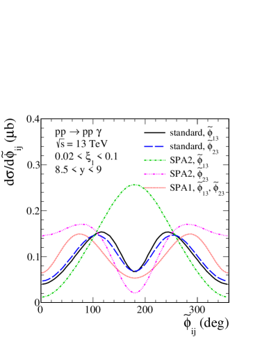
The azimuthal correlations between outgoing particles are particularly interesting. Figure 4 shows the distributions in defined as
| (14) |
In the left panel we show the results in , the angle between the transverse momenta of the outgoing protons, for our standard and SPA2 calculations. For SPA1 (not shown here) the outgoing protons are back-to-back, , i.e., the outgoing protons and the beam are in one plane . For our standard approach the main contribution is also placed at . The right panel of Fig. 4 shows the distributions in (), the azimuthal angles between the proton () and the photon . The SPA1 and our standard results show maxima for and around and . This corresponds to emission of the photon in a plane which is orthogonal to the plane . The SPA2 results for the and distributions deviate very significantly from our standard results.
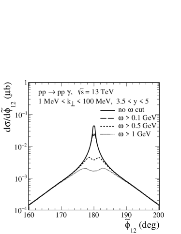
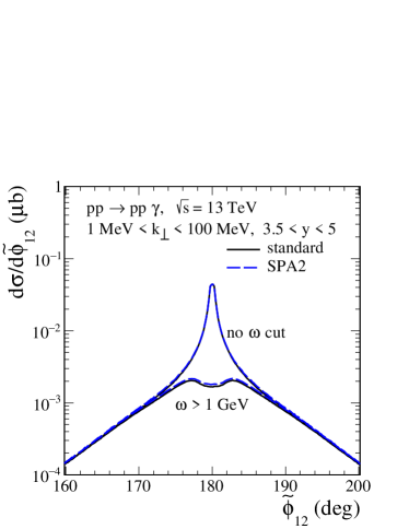
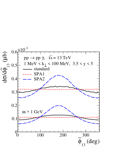
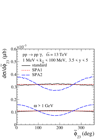
Here we will show also first predictions relevant for future experiment ALICE 3 [21]. Figure 5 shows the azimuthal distributions calculated for the photon rapidity , for the absolute value of the transverse momentum of the photon , and with various cuts on specified in the figure legends. The standard results are compared with those from the approximations, SPA1 and SPA2. The SPA1 and SPA2 results for and distributions deviate from the exact bremsstrahlung results, and it does not depend significantly on the cut on (see the bottom panels). For detailed comparisons of the predictions with experiment and in order to distinguish standard and the approximate results measurement of the outgoing protons would be welcome.
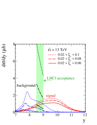
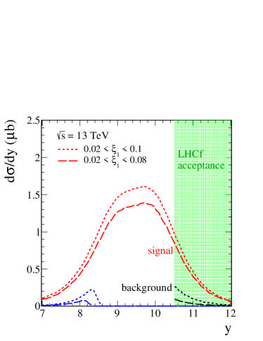
In Fig. 6 we show the result of a study of the background to our reaction . We take the upper estimate of the cross section for the reaction (Drell-Hiida-Deck type model) studied by two of us some time ago [13]. In the present calculations, we take the background corresponding to the form-factor parameters GeV and without absorption effects. The red lines represent the distributions of our (signal) standard bremsstrahlung of a single photon associated with a proton for which the fractional energy loss is in the intervals specified in the figure legend. In the left panel of Fig. 6, for the background contribution we assume that one photon is measured by the LHCf in the rapidity interval , GeV, and up to . The distributions of the measured photon correspond to the black lines (within the LHCf acceptance), while the distributions of the unmeasured photon correspond to the blue lines. The percentage of measured/unmeasured photons depends on the upper limit of . For (the solid lines) the second photon practically cannot be measured. The signal-to-background ratio for is somewhat larger than 1. In the right panel of Fig. 6, we present the contribution of the background for the LHCf acceptance range. Here, the signal-to-background ratio is of order of 4 for , and about 10 for .
We have estimated the coincidence cross section for the reaction only within the SPA1 approach. We have required that the final state protons and photons can be measured by the ATLAS forward proton (AFP) spectrometers and LHCf detectors, respectively. We have imposed the kinematical cuts , , , and obtained the cross section nb for TeV. Hopefully, our predictions will be verified by the ATLAS-LHCf measurement.
4 Conclusions
-
•
The calculations for the and reactions have been performed in the tensor-Pomeron model. We have studied single- and double-photon bremsstrahlung at very-forward/backward photon rapidities in proton-proton collisions at the LHC. We have compared our standard (complete) bremsstrahlung results and the results using the approximations SPA1 and SPA2.
-
•
We have studied the azimuthal angle correlations between outgoing particles. We observe very interesting correlations between protons and photons. Detailed comparisons of our predictions with experiments (ATLAS-LHCf, ALICE 3) in order to distinguish our complete and the approximate results measurement of the outgoing protons would be most welcome.
-
•
Experimental studies of one photon in collisions available at the ATLAS-LHCf measurement should provide new information about the exclusive diffractive contribution. We have briefly estimated the background contribution due to the diffractive process for single photon bremsstrahlung. We have compared the signal and background contributions in two LHCf acceptance regions. We conclude that there is a chance to measure single-photon bremsstrahlung.
-
•
The single photon bremsstrahlung mechanism should be identifiable by the measurement of proton and photon on one side by the ATLAS forward proton spectrometers (AFP) and LHCf detectors, respectively, and by checking the exclusivity condition (no particles in the main detector) without explicit measurement of the opposite side proton by AFP. Whether this is sufficient requires further studies, since such a measurement will probably include one-side diffractive dissociation, which can be of the order of 25%. The bremsstrahlung cross-section for two photons on different sides is rather small but should be measurable.
References
- [1] P. Lebiedowicz, O. Nachtmann, A. Szczurek, Phys. Lett. B 843, 138053 (2023).
- [2] P. Lebiedowicz, O. Nachtmann, A. Szczurek, Phys. Rev. D 106, 034023 (2022).
- [3] J. Chwastowski, A. Cyz, Ł. Fulek, R. Kycia, B. Pawlik, R. Sikora, J. Turnau, Acta Phys. Pol. B 46, 1979 (2015).
- [4] J. J. Chwastowski, S. Czekierda, R. Kycia, R. Staszewski, J. Turnau, M. Trzebiński, Eur. Phys. J. C 76, 354 (2016).
- [5] J. J. Chwastowski, S. Czekierda, R. Staszewski, M. Trzebiński, Eur. Phys. J. C 77, 216 (2017).
- [6] O. Adriani et al., arXiv:2203.15416 [hep-ex].
- [7] LHCf Collaboration, O. Adriani et al., Phys. Lett. B 780, 233 (2018).
- [8] LHCf Collaboration, A. Tiberio et al., PoS ICRC2023 (2023) 444.
- [9] P. Lebiedowicz, O. Nachtmann, A. Szczurek, Phys. Rev. D 105, 014022 (2022).
- [10] P. Lebiedowicz and A. Szczurek, Phys. Rev. D 87, 114013 (2013).
- [11] C. Ewerz, M. Maniatis, and O. Nachtmann, Annals Phys. 342, 31 (2014).
- [12] C. Ewerz, P. Lebiedowicz, O. Nachtmann, and A. Szczurek, Phys. Lett. B 763, 382 (2016).
- [13] P. Lebiedowicz and A. Szczurek, Phys. Rev. D 87, 074037 (2013).
- [14] P. Lebiedowicz, O. Nachtmann, A. Szczurek, Phys. Rev. D 93, 054015 (2016).
- [15] P. Lebiedowicz, O. Nachtmann, A. Szczurek, Phys. Rev. D 107, 074014 (2023).
- [16] P. Lebiedowicz, O. Nachtmann, A. Szczurek, arXiv:2307.13291 [hep-ph], accepted for publication in Phys. Rev. D.
- [17] S. Foroughi-Abari and A. Ritz, Phys. Rev. D 105, 095045 (2022).
- [18] C. S. Shin and S. Yun, JHEP 02, 133 (2022).
- [19] D. Gorbunov and E. Kriukova, JHEP 01, 058 (2024).
- [20] FASER Collaboration, H. Abreu et al., Phys. Lett. B 848, 138378 (2024).
- [21] ALICE Collaboration, arXiv: 2211.02491 [physics.ins-det].