Optimizing LiDAR Placements for Robust Driving Perception in Adverse Conditions

Abstract

The robustness of driving perception systems under unprecedented conditions is crucial for safety-critical usages. Latest advancements have prompted increasing interests towards multi-LiDAR perception. However, prevailing driving datasets predominantly utilize single-LiDAR systems and collect data devoid of adverse conditions, failing to capture the complexities of real-world environments accurately. Addressing these gaps, we proposed Place3D, a full-cycle pipeline that encompasses LiDAR placement optimization, data generation, and downstream evaluations. Our framework makes three appealing contributions. 1) To identify the most effective configurations for multi-LiDAR systems, we introduce a Surrogate Metric of the Semantic Occupancy Grids (M-SOG) to evaluate LiDAR placement quality. 2) Leveraging the M-SOG metric, we propose a novel optimization strategy to refine multi-LiDAR placements. 3) Centered around the theme of multi-condition multi-LiDAR perception, we collect a 364,000-frame dataset from both clean and adverse conditions. Extensive experiments demonstrate that LiDAR placements optimized using our approach outperform various baselines. We showcase exceptional robustness in both 3D object detection and LiDAR semantic segmentation tasks, under diverse adverse weather and sensor failure conditions. Code and benchmark toolkit are publicly available.

1 Introduction

(a) Waymo

(b) Motional

(c) Cruise

(d) Pony.ai

(e) Zoox

(f) Toyota

(g) Momenta

(h) Ford

Figure 1: A diverse spectrum of existing multi-LiDAR placement configurations employed by major autonomous vehicle companies [5, 4, 3, 2, 7, 8, 6, 1]. Images adopted from original websites.

Accurate 3D perception plays a crucial role in autonomous driving, involving detecting the objects around the vehicle and segmenting the scene into meaningful semantic categories. LiDARs are becoming crucial for driving perception due to their capability to capture detailed geometric information about the surroundings [11, 97]. While the latest models achieved promising accuracy on standard datasets, e.g., nuScenes [13], improving the robustness of perception under corruptions and sensor failures is still a critical yet under-explored task [46, 84].

Recent studies have primarily focused on refining the sensing systems by designing new algorithms with novel model architectures [19] or 3D representations [28, 88]. The selection of LiDAR configurations, however, often relies on industry experience and design aesthetics. Therefore, existing literature has potentially overlooked optimal LiDAR placements for maximum sensing efficacy.

An intuitive approach for optimizing LiDAR configurations involves a comprehensive cycle of data collection, model training, and validation across various LiDAR setups to enhance autonomous driving systems’ perception accuracy. However, this approach faces significant challenges due to the substantial computational resources and extensive time required for data collection and processing [53]. Although recent works [34, 60] made preliminary attempts to explore the impact of LiDAR placements on perception accuracy, they have neither proposed an optimization method nor evaluated the performance in adverse conditions.

In this work, we delve into the optimization of sensor configurations for autonomous vehicles by tackling two critical sub-problems: 1) the performance evaluation of sensor-specific configurations, and 2) the optimization of these configurations for enhanced 3D perception tasks, encompassing 3D object detection and LiDAR semantic segmentation. To achieve this goal, we propose a systematic LiDAR placements evaluation and optimization framework, dubbed Place3D. The overall pipeline is endowed with the capability to synthesize point cloud data with customizable configurations and diverse conditions, including common corruptions, external disturbances, and sensor failures.

We first introduce an easy-to-compute Surrogate Metric of Semantic Occupancy Grids (M-SOG) to evaluate the equality of LiDAR placements. Next, we propose a novel optimization approach utilizing our surrogate metric based on Covariance Matrix Adaptation Evolution Strategy (CMA-ES) to find the near-optimal LiDAR placements. To verify the correlation between our surrogate metric and assess the effectiveness of our optimization approach on both clean and adverse conditions, we design an automated multi-condition multi-LiDAR data simulation platform and establish a comprehensive benchmark consisting of a total of seven LiDAR placement baselines inspired by existing self-driving configuration from the autonomous vehicle companies (cf. Fig. 1).

Our benchmark, along with a large-scale multi-condition multi-LiDAR perception dataset, encompasses state-of-the-art learning-based perception models for 3D object detection [50, 95, 58, 97] and LiDAR semantic segmentation [21, 99, 78, 105], as well as six distinct adverse conditions coped with weather and sensor failures. Utilizing the proposed Place3D framework, we explored how various perturbations and downstream 3D perception tasks affect optimization outcomes. To summarize, this work makes the following key contributions:

• To the best of our knowledge, Place3D serves as the first attempt at investigating the impact of multi-LiDAR placements in diverse conditions.

• We introduce M-SOG, an innovative surrogate metric to effectively evaluate the quality of LiDAR placements for both detection and segmentation tasks.

• We propose a novel optimization approach utilizing our surrogate metric to refine LiDAR placements, which exhibit excellent 3D perception accuracy and robustness, outperforming baselines for up to 9% scores.

• We contribute a 364,000-frame multi-condition multi-LiDAR point cloud dataset and establish a comprehensive benchmark for the 3D robustness evaluation. We hope this work can lay a solid foundation for future research.

2 Related Work

LiDAR Sensing. LiDAR sensing plays a vital role in advanced autonomous vehicles, acquiring structural information from the surroundings and serving as the most critical components for their operation [55, 11, 66]. Leveraging its 3D data, LiDAR enables a variety of tasks designed to meet practical needs. Prominent among these tasks include perception [13, 27, 29, 12, 77, 48], generation [68, 106, 67, 86], decision making [26, 14, 22, 79], and simulation [25, 63, 62, 83]. This work specifically targets LiDAR-based perception and simulation, which are at the forefront of current research in autonomous vehicle technology.

LiDAR Semantic Segmentation. As one of the most crucial tasks in LiDAR-based perception, LiDAR segmentation has attracted wide research attention. Based on representations of LiDAR points, the LiDAR segmentation models can be categorized into point-based [80, 35, 36, 98, 69], range view [65, 81, 24, 87, 101, 20, 47, 9, 45, 88], bird’s eye view [99, 103, 16], voxel-based [21, 78, 105, 33], and multi-view fusion [54, 38, 70, 56, 57, 18, 17] methods. Albeit achieving promising results on standard LiDAR semantic segmentation benchmarks, their performance across various LiDAR sensor configurations has not been thoroughly explored. In this work, we conduct the first study to examine how different LiDAR placements affect the effectiveness of state-of-the-art LiDAR segmentation algorithms.

3D Object Detection. Another critical task for driving perception aims to locate and classify road participants in 3D scenes [10]. Most prevailing 3D object detection models adopt point-based [74, 94, 93, 104] or voxel-based [102, 50, 64, 82, 75, 51, 61, 92] representations. Recently, there has been a shift towards fusing both approaches for improved detection performance [59, 72, 73, 58, 52]. Our study is perpendicular to existing 3D object detection approaches. We find that strategically optimized LiDAR placements can significantly enhance 3D object detection performance under a variety of real-world sensing conditions.

Perception Robustness. The reliability of perception models is crucial for driving applications in real-world scenarios [76, 39]. Recently, several studies explored the robustness of 3D perception models against adversarial attacks [100, 85], common corruptions [46, 49, 84, 91, 43], adverse weather conditions [31, 30, 71, 37], sensor failures [96, 19, 28], and combined motion and sensor perturbations [90]. To the best of our knowledge, no prior work has specifically targeted optimizing the placement of LiDAR sensors to improve 3D robustness. Our Place3D fills this gap by introducing a comprehensive study of different placement strategies against both in-domain and out-of-domain scenarios, which could inspire future exploration in optimizing sensor configurations to fortify perception robustness.

Sensor Placement Optimization. Optimizing sensor placements can alleviate the challenges of heuristic design and significantly enhance performance [42, 89]. In the realm of autonomous driving, optimizing LiDAR sensor placements represents a relatively new field study[60]. Hu et al. [34] presented the first study on optimizing multi-LiDAR placements for 3D object detection. Li et al. [53] focused on the influence of LiDAR-camera configurations on multi-modal 3D object detection. Several other works [41, 44, 15, 40] explored the placements of roadside LiDAR sensors for vehicle-to-everything applications, diverging from the focus on in-vehicle perception. Distinguishing from previous efforts, our work makes the first attempt at investigating LiDAR placements for robust 3D perception in challenging conditions. We establish comprehensive benchmarks for both LiDAR semantic segmentation and 3D object detection and perform in-depth analysis on the optimization of LiDAR placements for robust perception.

3 Place3D

In this section, we introduce the Surrogate Metric of Semantic Occupancy Grids (M-SOG) to assess the 3D perception performance of sensor configurations (cf. Sec. 3.1). Leveraging M-SOG, we propose a novel optimization strategy for multi-LiDAR placement (cf. Sec. 3.2). Our approach is theoretically grounded; we provide an optimality certification to ensure that optimized placements are close to the global optimum (cf. Sec. 3.3). Fig. 2 depicts an overview of our framework.

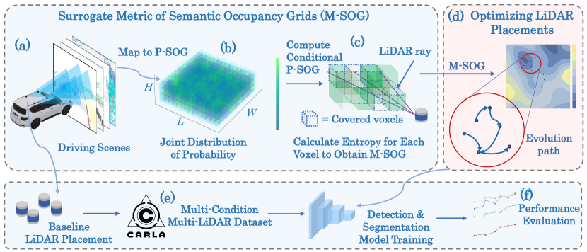
Figure 2: Place3D pipeline for multi-LiDAR placement optimization. We first generate Probabilistic SOG (b) by merging multiple frames of data synthesized in CARLA into dense point cloud (a) and obtain voxels covered by LiDAR rays to compute the Surrogate Metric of Semantic Occupancy Grids (M-SOG) based on the joint probability distribution of covered voxels (c). We propose a CMA-ES-based optimization strategy to maximize M-SOG, finding optimal LiDAR placement (d). To verify the effectiveness of our optimization strategy, we contribute a multi-condition multi-LiDAR dataset (e). We train several state-of-the-art models and evaluate the performance of baseline and optimized placements on both clean and corruption data (f). Our optimized placement generally outperforms all baseline placements in experiments.

3.1 M-SOG: Surrogate Metric of Semantic Occupancy Grids

Region of Interest. We first define the Region of Interest (ROI) for perception as a finite 3D cuboid space $[L,W,H]$ with ego-vehicle in the center and divide the ROI space $S$ into voxels with resolution [$\delta_{L},\delta_{W},\delta_{H}$] as $S=\{v_{1},v_{2},...,v_{N}\}$, where $N=\frac{L}{\delta_{L}}\times\frac{W}{\delta_{W}}\times\frac{H}{\delta_{H}}$ denotes the total number of voxelized grids.

Semantic Occupancy Grids (SOG). Given a 3D scene with a set of semantic labels $Y=\{y_{1},y_{2},...,y_{K}\}$, where $K$ represents the total number of object classes in the scene and assuming that each voxel can only be occupied by one semantic tag for each frame, we denote $y^{(t)}(v_{i})$ as the semantic label of voxel $v_{i}\in\{v_{1},v_{2},...,v_{N}\}$ at time frame $t\in\{1,2,...,T\}$. Accordingly, the set of voxels occupied by semantic label $y_{k}$ at frame $t$ is defined as $s_{y_{k}}^{(t)}=\{v_{i}|y^{(t)}(v_{i})=y_{k}\},\;k=1,2,...,K,\;t=1,2,...,T$. Then, we introduce the Semantic Occupancy Grids to describe the total semantic voxel distribution,

$$S_{SOG}^{(t)}=\{s_{y_{1}}^{(t)},s_{y_{2}}^{(t)},...,s_{y_{K}}^{(t)}\},\;t=1,2,...,T~{}.$$ (1)

Probabilistic SOG. We propose P-SOG $p_{SOG|y_{k}}=p\{v_{1},v_{2},...,v_{N}|y_{k}\}$ to describe the joint probability distribution of voxels belonging to certain semantic labels. Before estimating $p_{SOG|y_{k}}$, we first traverse all frames from given scenes to obtain the probability $\hat{p}$ for each voxel $v_{i}$ occupied by each semantic label:

$$\hat{p}(v_{i}|y_{k})=\frac{\sum_{t=1}^{T}\mathds{1}(v_{i}\in s_{y_{k}}^{(t)})}{T}~{},$$ (2)

where $\mathds{1}(\cdot)$ serves as an occupancy indicator function. Notably, $\hat{p}$ indicates estimated distributions from observed samples, whereas $p$ refers to the statistical parameters to be estimated, which are unknown and non-random. We compute the joint probability of all non-zero voxels for semantic label $y_{k}$ in the ROI to estimate the $p_{SOG|y_{k}}$. Recognizing that an object’s presence in one voxel does not imply its presence in others, we treat voxels as independent, identically distributed variables, calculating the joint distribution over the ROI set $S$ as:

$$\hat{p}_{SOG|y_{k}}=\hat{p}(v_{1},v_{2},...,v_{N}|y_{k})=\prod_{i=1,\;\hat{p}(v_{i}|y_{k})\neq 0}^{N}{\hat{p}(v_{i}|y_{k})}~{}.$$ (3)

Conditional P-SOG. To evaluate LiDAR placements, we further analyze the joint probability distribution of voxels covered by LiDAR rays. Leveraging the Bresenham’s Line Algorithm, we obtain the voxels covered by LiDAR rays given LiDAR configuration $L=L_{j}$, $j=1,2,...,J$ as $S|L_{j}=Bresenham(S,L_{j})=\{v_{1}^{L_{j}},v_{2}^{L_{j}},...,v^{L_{j}}_{N_{j}}\}$, where $J$ is the number of total potential configurations and $N_{j}$ is the number of voxels covered by rays of LiDAR Configuration $L=L_{j}$. Then we have the conditional P-SOG $\hat{p}_{SOG|y_{k},L_{j}}=\hat{p}(v_{1}^{L_{j}},v_{2}^{L_{j}},...,v_{N}^{L_{j}}|y_{k})$. From the perspective of density estimation to find the P-SOG of the semantic object $y_{k}$, the P-SOG and conditional P-SOG can be estimated as $p_{SOG|y_{k}}=\hat{p}_{SOG|y_{k}},p_{SOG|y_{k},L_{j}}=\hat{p}_{SOG|y_{k},L_{j}}$, respectively.

Figure 3: Pipeline of probabilistic SOG generation. We generate dense point clouds (b) by merging multiple frames of raw point clouds (a). Then, we voxelize the dense point clouds into Semantic Occupancy Grids (SOG) (c), and traverse all frames of dense point cloud to compute Probabilistic Semantic Occupancy Grids (P-SOG) (d).

Surrogate Metric of SOG (M-SOG). Entropy can be used to describe the uncertainty, indicating the perception capability of sensors. To this end, we calculate the entropy for each voxel, i.e., $\hat{H}(v_{i})=-\sum_{k=1}^{K}\hat{p}(v_{i}|y_{k})\log\hat{p}(v_{i}|y_{k})$. Then, we obtain the total entropy of P-SOG and conditional P-SOG as follows:

$$H_{SOG}=H(S) =\mathds{E}_{v_{i}\sim p_{S}}\sum_{i=1}^{N}\hat{H}(v_{i})~{},$$ (4)

$$H_{SOG|L_{j}}=H(S|L_{j}) =\mathds{E}_{v_{i}^{L_{j}}\sim p_{S|L_{j}}}\sum_{i=1}^{N_{j}}\hat{H}(v_{i}^{L_{j}})~{}.$$ (5)

We further define the Information Gain $IG_{S|L_{j}}=\frac{H(S)}{N}-\frac{H(S|L_{j})}{N_{j}}$ given LiDAR configuration $L_{j}$ to describe the difference between the mean values of entropy of P-SOG and conditional P-SOG. Since $\frac{H(S)}{N}$ is a constant given certain scenes with fixed P-SOG distribution, we propose the Surrogate Metric of Semantic Occupancy Grids (M-SOG) as follows to evaluate the perception capability:

$$\mathbf{M}_{SOG}(L_{j})=-\frac{H(S|L_{j})}{N_{j}}~{}.$$ (6)

3.2 Sensor Configuration Optimization

Algorithm 1 Multi-LiDAR Placement Optimization

1:Initialize: $k\leftarrow 0$, $\mathbf{m}^{(0)}$, $\sigma^{(0)}$, $\mathbf{C}^{(0)}$, $N_{k}$, $M_{k}$, $\forall k\in\{0,1,2,\dots,K\}$

2:for $k=0,1,2,\ldots,K$ do

3:     for $i=1$ to $N_{k}$ do

4:         Sample $\mathbf{u}_{i}^{(k)}\sim\mathcal{N}(\mathbf{m}^{(k)},(\sigma^{(k)})^{2}\mathbf{C}^{(k)})$ from $\delta$-density gird-level candidates

5:         Calculate $G(\mathbf{u}_{i}^{(k)})$

6:     end for

7:     Update $\mathbf{m}^{(k+1)}$ based on the top $M_{k}$ best solutions $\hat{\mathbf{u}}_{i}^{(k)}$ via Eqn. (7)

8:     Update $\sigma^{(k+1)}$ and $\mathbf{C}^{(k+1)}$ via Eqn. (8), (9), (10), and (11)

9:end for

We adopt the heuristic optimization based on the Covariance Matrix Adaptation Evolution Strategy (CMA-ES) [32] to find an optimized LiDAR configuration.

Objective Function. We define the objective function as $F(\mathbf{u}_{j})=\mathbf{M}_{SOG}(L_{j})$, where $\mathbf{u}_{j}\in\mathcal{U}\subset\mathbb{R}^{n}$ represents the LiDAR configuration $L_{j}$ and is subject to the physical constraint $P(\mathbf{u}_{j})=0$, and $P(\mathbf{u})>0$ if it is violated, e.g., mutual distance between LiDARs and distance from a 2D plane. Without ambiguity, we omit subscript $j$ in the following text. We then transform the constrained optimization into the unconstrained Lagrangian form as $G(\mathbf{u})=-F(\mathbf{u})+\lambda P(\mathbf{u})$, where $\lambda$ is the Lagrange multiplier. We optimize $G(\mathbf{u})$ through an iterative process that adapts the distribution of candidate solutions as Algorithm 1.

Optimization Approach. We first define a multivariate normal distribution $\mathcal{N}(\mathbf{m}^{(k)},(\sigma^{(k)})^{2}\mathbf{C}^{(k)})$, where $\mathbf{m}^{(k)}$, $\sigma^{(k)}$, and $\mathbf{C}^{(k)}$ are the mean vector, step size, and covariance matrix of the distribution of iteration $k$, respectively. We discretize the configuration space $\mathcal{U}$ with density $\delta$ and sample $N_{k}$ candidates $u_{i}^{(k)}\sim\mathcal{N}(\mathbf{m}^{(k)},(\sigma^{(k)})^{2}\mathbf{C}^{(k)})$ in each iteration $k$. We update mean vector $\mathbf{m}^{k+1}$ for the next iteration $k+1$ as the updated center of the search distribution for LiDAR configuration. The overall process can be depicted as follows:

$$\mathbf{m}^{(k+1)}=\sum_{i=1}^{M_{k}}w_{i}\hat{\mathbf{u}}_{i}^{(k)},\;G(\hat{\mathbf{u}}_{1}^{(k)})\leq G(\hat{\mathbf{u}}_{2}^{(k)})\leq\dots\leq G(\hat{\mathbf{u}}_{M_{k}}^{(k)})~{},$$ (7)

where $M_{k}$ is the number of best solutions we adopt to generate $\mathbf{m}^{(k+1)}$, and $w_{i}$ are the weights based on solution fitness. We obtain the evolution path $\mathbf{p}_{\mathbf{C}}^{(k+1)}$ that accumulates information about the direction of successful steps as follows:

$$\mathbf{p}_{\mathbf{C}}^{(k+1)}=(1-c_{\mathbf{C}})\cdot\mathbf{p}_{\mathbf{C}}^{(k)}+\sqrt{1-(1-c_{\mathbf{C}})^{2}}\cdot\sqrt{\frac{1}{\sum_{i=1}^{M_{k}}w_{i}^{2}}}\cdot\frac{\mathbf{m}^{(k+1)}-\mathbf{m}^{(k)}}{\sigma^{(k)}}~{},$$ (8)

where $c_{\mathbf{C}}$ is the learning rate for the covariance matrix update. The covariance matrix $\mathbf{C}$ controls the shape and orientation of the search distribution for LiDAR configurations. It can be updated at each iteration $k$ in the following format:

$$\mathbf{C}^{(k+1)}=(1-c_{\mathbf{C}})\mathbf{C}^{(k)}+c_{\mathbf{C}}\mathbf{p}_{\mathbf{C}}^{(k+1)}{\mathbf{p}_{\mathbf{C}}^{(k+1)}}^{T}~{},$$ (9)

Similarly, we update $\mathbf{p}_{\sigma}$ as the evolution path for step size adaptation. Then, the global step size $\sigma$ can be found below for the scale of search to balance exploration and exploitation:

$$\mathbf{p}_{\sigma}^{(k+1)}=(1-c_{\sigma})\mathbf{p}_{\sigma}^{(k)}+\sqrt{1-(1-c_{\sigma})^{2}}\cdot\sqrt{\frac{1}{\sum_{i=1}^{M_{k}}w_{i}^{2}}}\cdot\frac{\mathbf{m}^{(k+1)}-\mathbf{m}^{(k)}}{\sigma^{(k)}}~{},$$ (10)

$$\sigma^{(k+1)}=\sigma^{(k)}\exp\left(\frac{c_{\sigma}}{d_{\sigma}}\left(\frac{\|\mathbf{p}_{\sigma}^{(k+1)}\|}{E\|\mathcal{N}(0,\mathbf{I})\|}-1\right)\right)~{},$$ (11)

where $c_{\sigma}$ is the learning rate for updating the evolution path $\mathbf{p}_{\sigma}$. $d_{\sigma}$ is a normalization factor to calibrate the pace at which the global step size is adjusted.

3.3 Theoretical Analysis

Once the evolution optimization empirically converges, it holds that the optimized solution is the local optima of the $\delta$-density Grids space of LiDAR configuration space. In this section, we provide a stronger optimality certification to theoretically ensure that the optimized placement is close to the global optimum.

Theorem 3.1 (Optimality Certification)

Given the continuous objective function $G:\mathbb{R}^{n}\to\mathbb{R}$ with Lipschitz constant $k_{G}$ w.r.t. input $\textbf{u}\in\mathcal{U}\subset\mathbb{R}^{n}$ under $\ell_{2}$ norm, suppose over a $\delta$-density Grids subset $S\subset\mathcal{U}$, the distance between the maximal and minimal of function $G$ over $S$ is upper-bounded by $C_{M}$, and the local optima is $\textbf{u}^{*}_{S}=\arg\min_{\textbf{u}\in S}G(x)$, the following optimality certification regarding $x\in\mathcal{U}$ holds that:

$$\|G(\textbf{u}^{*})-G(\textbf{u}^{*}_{S})\|_{2}\leq C_{M}+k_{G}\delta~{},$$ (12)

where $\textbf{u}^{*}$ is the global optima over $\mathcal{U}$.

Proof

For the $\delta$-density subset $S\subset\mathcal{U}$, it holds that $\forall\textbf{u}\in\mathcal{U}$, $\min_{\textbf{u}_{S}\in S}\|\textbf{u}-\textbf{u}_{S}\|_{2}\leq\delta$. By the Lipschitz condition, we have $\|G(\textbf{u}_{1})-G(\textbf{u}_{2})\|_{2}\leq k_{G}\|\textbf{u}_{1}-\textbf{u}_{2}\|_{2},\forall\textbf{u}_{1},\textbf{u}_{2}\in B$. By the bounded fluctuation of $G$ over $S$, it holds that $\|G(\textbf{u}_{1})-G(\textbf{u}_{2})\|_{2}\leq\|\max_{\textbf{u}\in S}G(\textbf{u})-\min_{\textbf{u}\in S}G(\textbf{u})\|_{2}\leq C_{M},\forall\textbf{u}_{1},\textbf{u}_{2}\in S$. Therefore, by absolute value inequality, we have:

$$\|G(\textbf{u}^{*})-G(\textbf{u}^{*}_{S})\|_{2}~{}\leq~{} \|G(\textbf{u}^{*})-G(\textbf{u}_{S})\|_{2}+\|G(\textbf{u}^{*})-G(\textbf{u}_{S})\|_{2}$$ (13)

$$~{}\leq~{} k_{G}(\textbf{u}^{*}-\textbf{u}_{S})+C_{M}~{},$$ (14)

where there exists a candidate $\textbf{u}_{S}$ that is subject to the condition $(\textbf{u}^{*}-\textbf{u}_{S})\leq\delta$, which concludes the proof by combining the above inequality. $\blacksquare$

The global optimality certification Theorem 3.1 is applicable in practice because the Lipschitz constant $k_{G}$ and the distance between the maximal and minimal of objective function $G$ over $S$ can be approximated easily through calculating $G(\textbf{u}_{i}^{(k)})$ of Algorithm 1 for each sampled $\textbf{u}_{i}^{(k)}$ over the $\delta$-density Grids subset. Besides, we have a more general remark below to further relax the assumption. The full proof can be found in the supplementary materials.

Remark 1

When $\mathcal{U}$ is a hyper-rectangle with the bounded $\ell_{2}$ norm of domain $U_{i}\in\mathbb{R}$ at each dimension $i$, with $i=1,2,\dots,n$, we remark Theorem 3.1 can hold in a more general way by only assuming that the Lipschitz constant $k_{G}$ of the objective function is given, where Eq. 12 becomes:

$$\|G(\textbf{u}^{*})-G(\textbf{u}^{*}_{S})\|_{2}\leq k_{G}\sum_{i=1}^{n}{U_{i}}+k_{G}\delta~{}.$$ (15)

4 Experiments

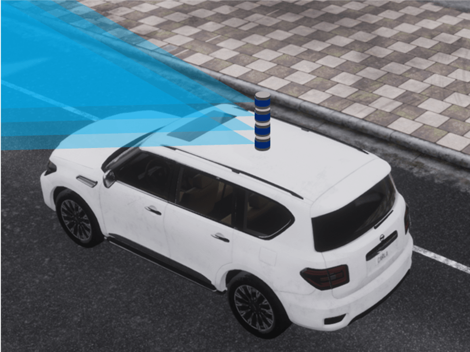
(a) Center

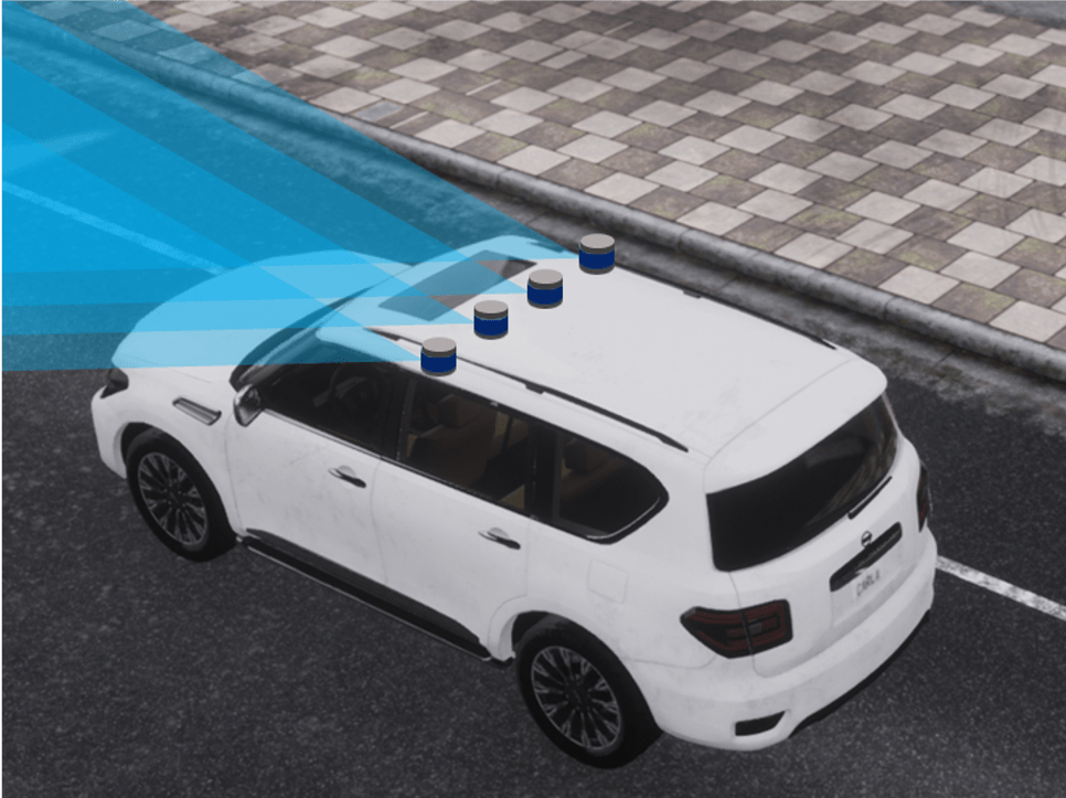
(b) Line

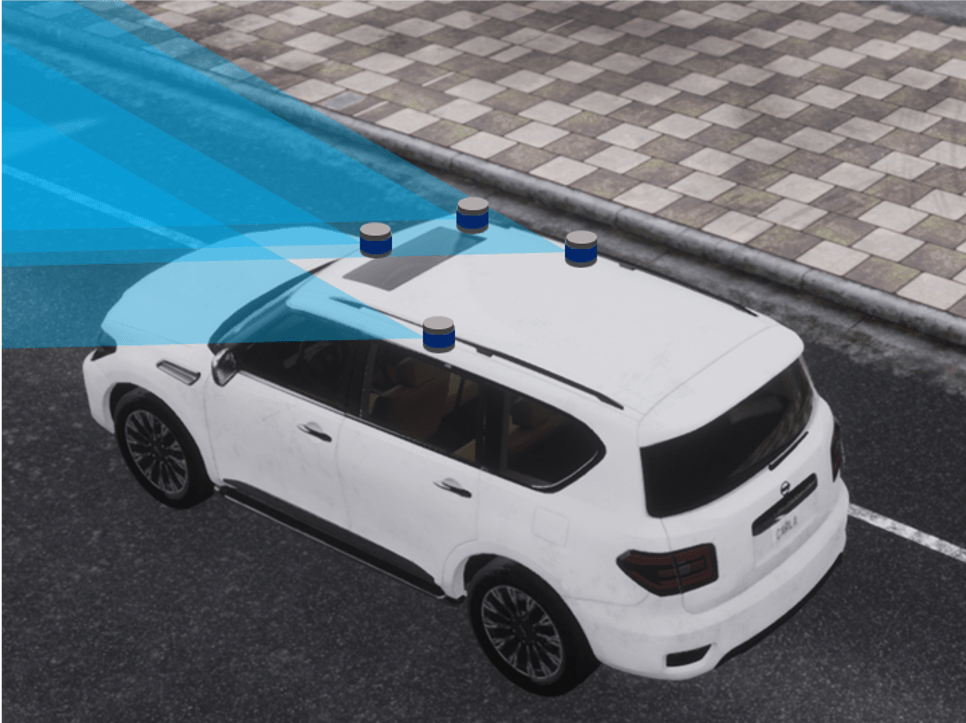
(c) Pyramid

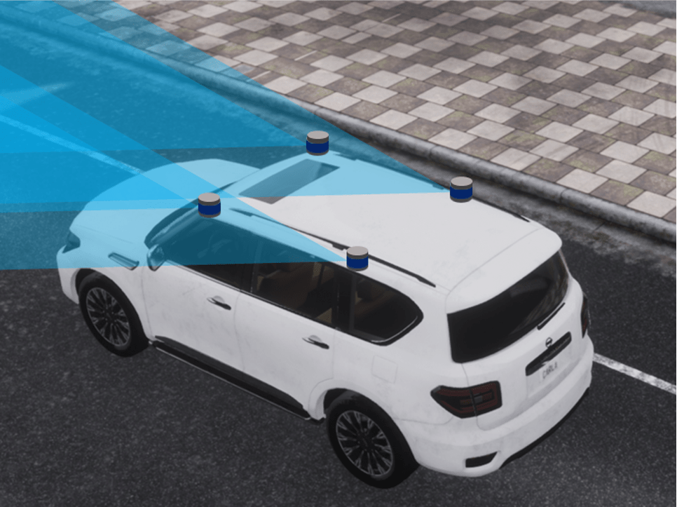
(d) Square

(e) Trapezoid

(f) Line-roll

(g) Ours (Det)

(h) Ours (Seg)

Figure 4: Visualized LiDAR Placements. We compare the placements optimized from our proposed M-SOG metric (for both detection and segmentation tasks) and heuristic LiDAR placements utilized by major autonomous vehicle companies (cf. Fig. 1).

Table 1: Optimized M-SOG Metrics. We report $\mathbf{M}_{SOG}$ scores for both tasks. The scores are calculated based on the car class for detection and all semantic classes for segmentation. Line-roll and Pyramid-roll are abbreviated as L-roll and P-roll.

Metrics [$\mathbf{M}_{SOG}$]	Center	Line	Pyramid	Square	Trapezoid	L-roll	P-roll	Ours
3D Detection ($\times 10^{-6}$)	$-1.26$	$-1.65$	$-1.34$	$-1.54$	$-1.52$	$-1.41$	$-1.35$	$-1.18$
3D Segmentation ($\times$ $10^{-6}$)	$-1.58$	$-2.62$	$-2.56$	$-2.35$	$-2.89$	$-3.13$	$-1.63$	$-1.29$

4.1 Benchmark Setups

Data Generation. We generate LiDAR point clouds and the corresponding ground truth using the CARLA simulator [25]. Following previous literature [34], we use the maps of Towns 1, 3, 4, and 6 and set 6 ego-vehicle routes for each map. We incorporate 23 semantic classes for LiDAR semantic segmentation and 3 classes of objects for 3D object detection (Car, Bicycle, and Pedestrian). For each LiDAR configuration, the sub-dataset consists of 13,600 frames of samples, comprising 11,200 samples for training and 2,400 samples for validation, following the split ratio used in nuScenes [13]. More details are in the Appendix.

Corruption Types. To replicate adverse conditions, we synthesized six types of corrupted point clouds on the validation set of each sub-set, following the settings of the Robo3D benchmark [46]. These corruptions can be categorized into three groups: 1) Severe Weather Conditions, including fog, snow, and wet ground; 2) External Disturbances, such as motion blur; and 3) Internal Sensor Failure, including crosstalk and incomplete echo. See Appendix for more details.

Multi-LiDAR Configurations. We adopt five commonly employed heuristic LiDAR placements, which have been adopted by several leading autonomous driving companies, as our baseline. These placements are represented in Fig. 4a-e. Following the KITTI dataset [29], we configured the LiDAR sensor with a vertical field of view (FOV) of [-24.8, 2.0] degrees. To achieve the Line-roll and Pyramid-roll configurations, we adjusted the roll angles of the LiDARs for both the Line and Pyramid setups. The Line-roll configuration is depicted in Fig. 4.

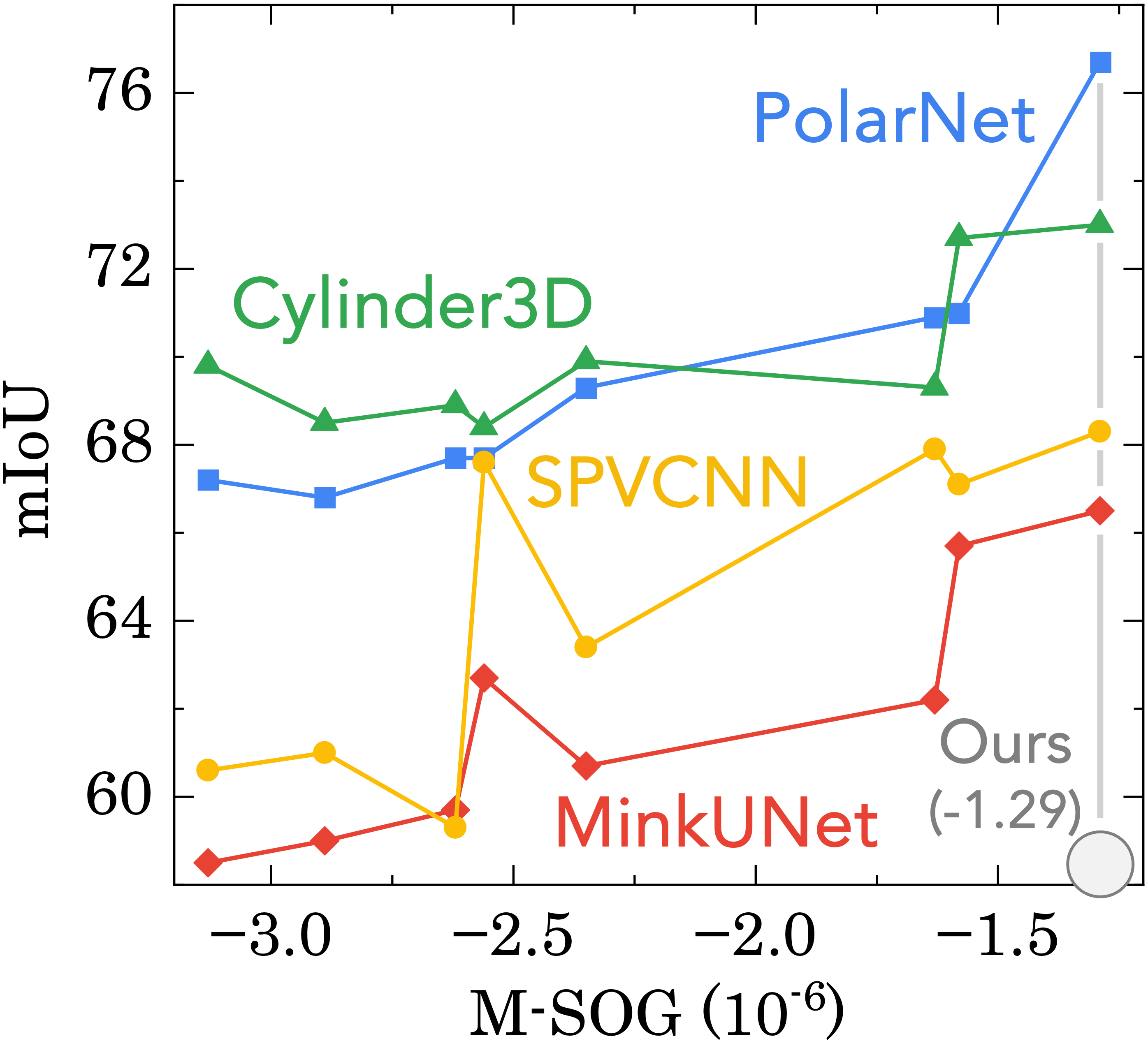
(a) Clean (Seg)

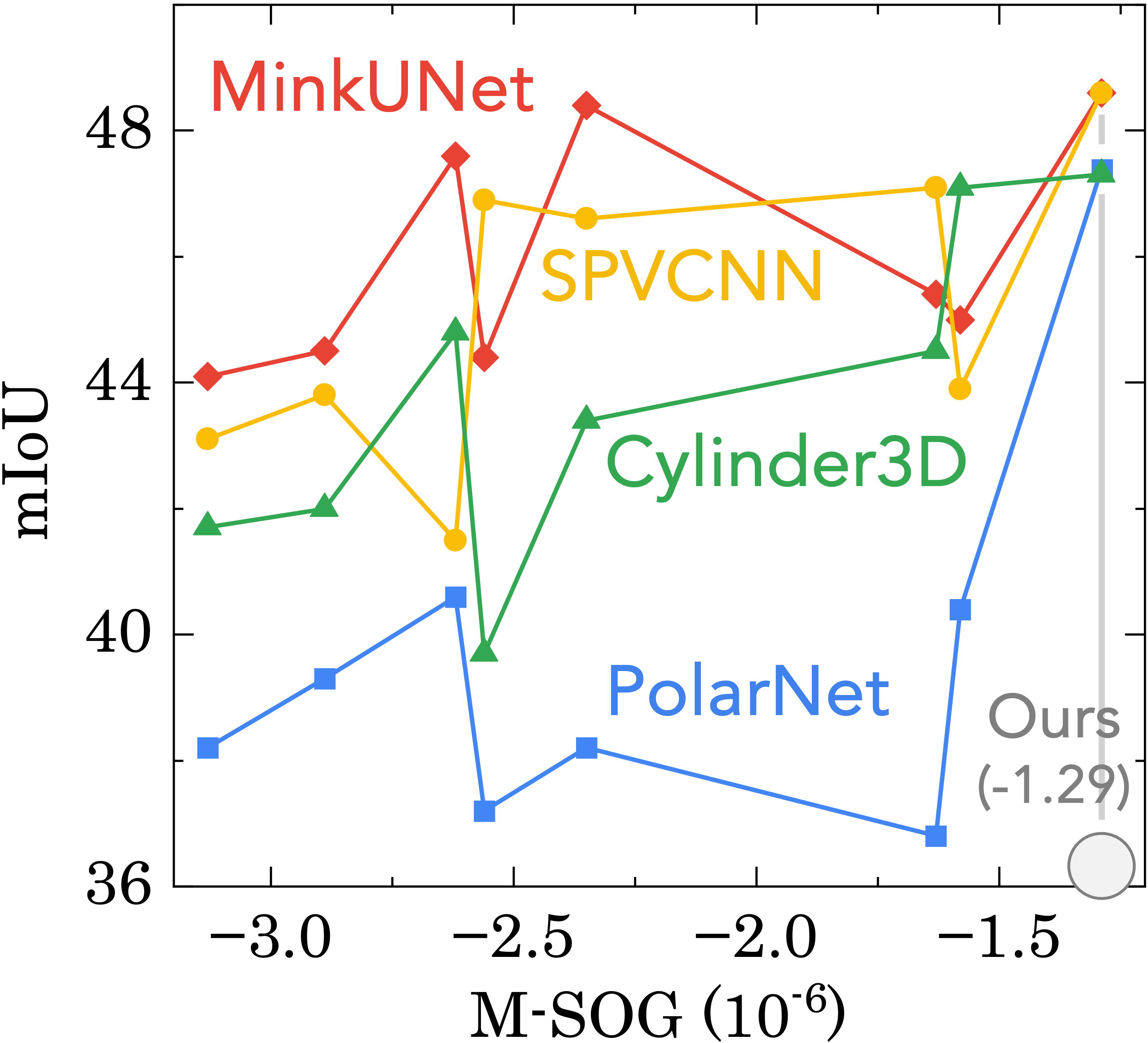
(b) Corruptions (Seg)

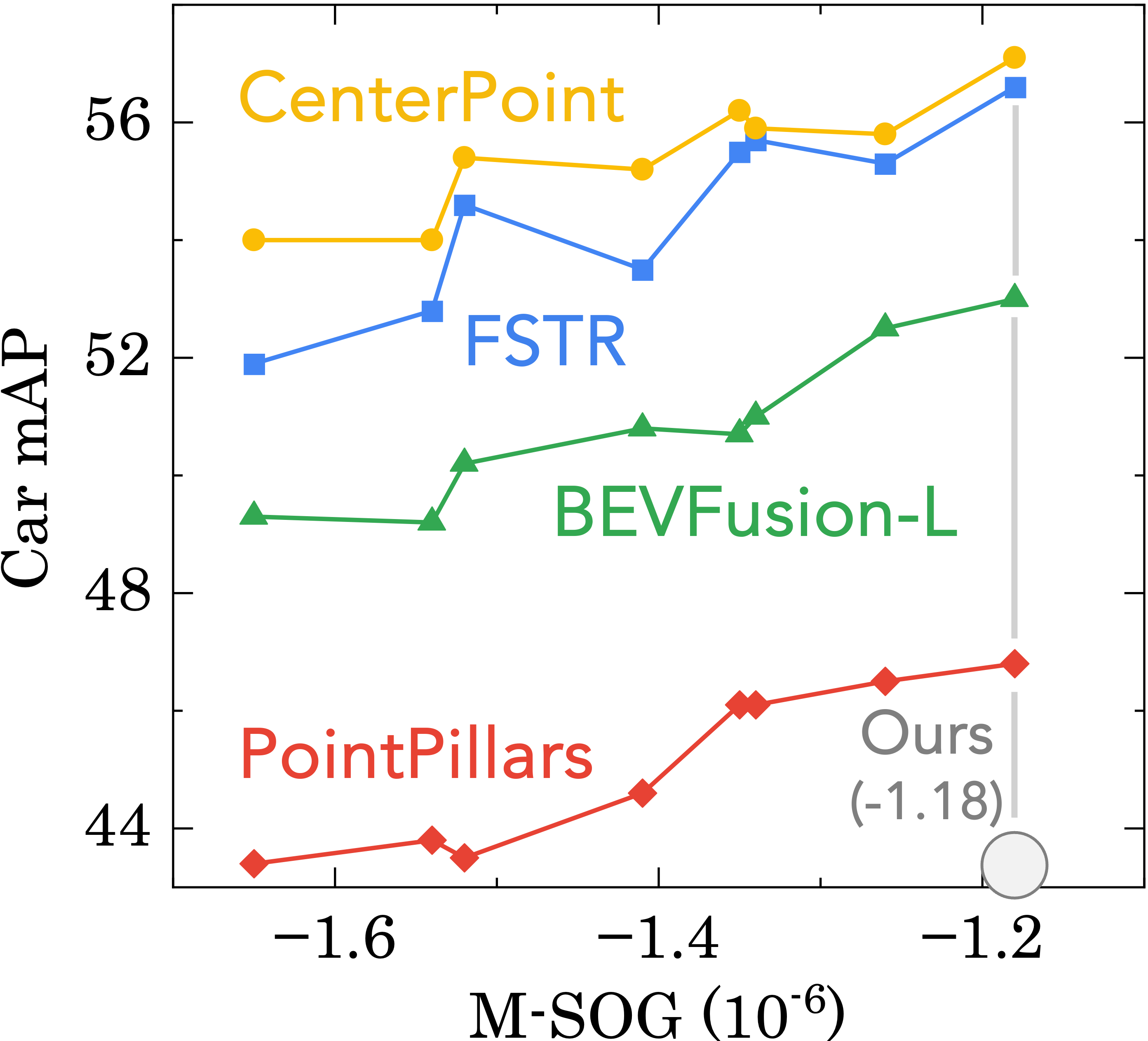
(c) Clean (Det)

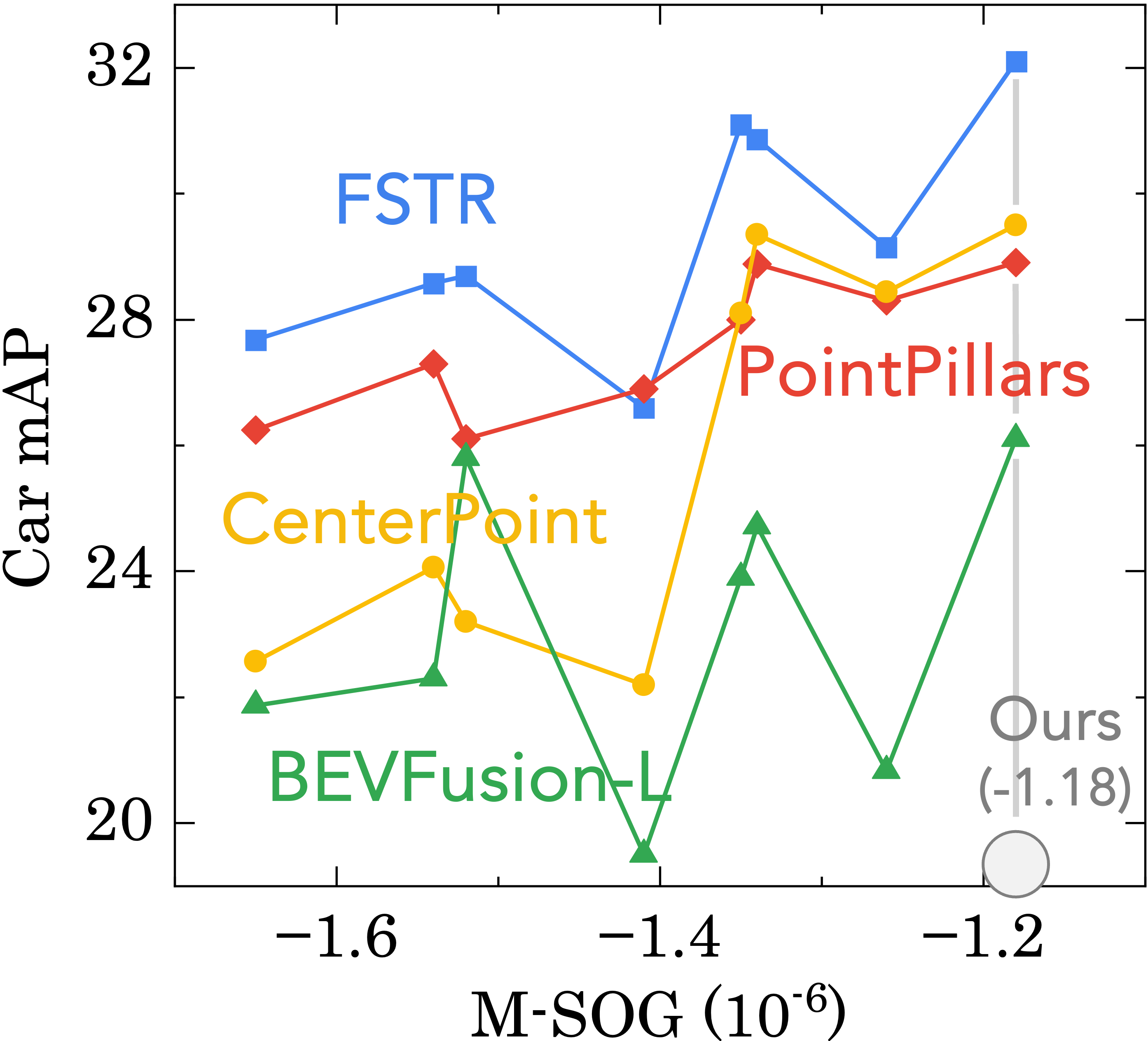
(d) Corruptions (Det)

Figure 5: The relationship between perception performance and M-SOG, separated for the LiDAR semantic segmentation (a & b) and 3D object detection (c & d) tasks. Notably, we report true scores in clean condition and average scores under corruptions.

SOG Synthesis. We follow the steps as depicted in Fig. 3 to synthesize the semantic occupancy grids for each scene. We first collect point clouds and semantic labels using one high-resolution LiDAR in CARLA and sequentially divide all samples into multiple subsets. Through the transformation of world coordinates of the ego-vehicle, frames of point clouds of each subset are aggregated into one frame of dense point cloud. Then, we utilize the voting strategy to determine the semantic label for each voxel in ROI and generate the SOG. This process is executed across all subsets to produce P-SOG. Notably, the P-SOG is only generated on the scenes of the training set.

Surrogate Metric of SOG. We compute the scores of M-SOG separately for detection and segmentation, as shown in Tab. 1. To evaluate M-SOG for segmentation, we utilize all semantic classes to generate the semantic occupancy grid. For detection, we specifically focus on the car semantic type, while merging the remaining semantic types into a single category for M-SOG analysis.

Table 2: Benchmark results of LiDAR semantic segmentation under clean condition. For each LiDAR placement, we report the mIoU ($\uparrow$), mAcc ($\uparrow$), and ECE ($\downarrow$) scores. The mIoU and mAcc scores are given in percentage ($\%$).

Method	Center			Line			Pyramid			Square
	mIoU	mAcc	ECE	mIoU	mAcc	ECE	mIoU	mAcc	ECE	mIoU	mAcc	ECE
MinkUNet [21]	$65.7$	$72.4$	$0.041$	$59.7$	$67.7$	$0.037$	$62.7$	$70.6$	$0.072$	$60.7$	$68.4$	$0.043$
PolarNet [99]	$71.0$	$76.0$	$0.033$	$67.7$	$74.1$	$0.034$	$67.7$	$73.0$	$0.032$	$69.3$	$74.7$	$0.033$
SPVCNN [78]	$67.1$	$74.4$	$0.034$	$59.3$	$66.7$	$0.068$	$67.6$	$74.0$	$0.037$	$63.4$	$70.2$	$0.031$
Cylinder3D [105]	$72.7$	$79.2$	$0.041$	$68.9$	$76.3$	$0.045$	$68.4$	$76.0$	$0.093$	$69.9$	$76.7$	$0.044$
Average	$69.1$	$75.5$	$0.037$	$63.9$	$71.2$	$0.046$	$66.6$	$73.4$	$0.059$	$65.8$	$72.5$	$0.038$
Method	Trapezoid			Line-Roll			Pyramid-Roll			Ours
	mIoU	mAcc	ECE	mIoU	mAcc	ECE	mIoU	mAcc	ECE	mIoU	mAcc	ECE
MinkUNet [21]	$59.0$	$66.2$	$0.040$	$58.5$	$66.4$	$0.047$	$62.2$	$69.6$	$0.051$	$66.5$	$73.2$	$0.031$
PolarNet [99]	$66.8$	$72.3$	$0.034$	$67.2$	$72.8$	$0.037$	$70.9$	$75.9$	$0.035$	$76.7$	$81.5$	$0.033$
SPVCNN [78]	$61.0$	$68.8$	$0.044$	$60.6$	$68.0$	$0.034$	$67.9$	$74.2$	$0.033$	$68.3$	$74.6$	$0.034$
Cylinder3D [105]	$68.5$	$75.4$	$0.057$	$69.8$	$77.0$	$0.048$	$69.3$	$77.0$	$0.048$	$73.0$	$78.9$	$0.037$
Average	$63.8$	$70.7$	$0.044$	$64.0$	$71.1$	$0.042$	$67.6$	$74.2$	$0.042$	$71.1$	$77.1$	$0.034$

Table 3: Benchmark results of 3D object detection under clean condition. For each LiDAR placement, we report the mAP ($\uparrow$) scores (for car, pedestrian, and bicyclist classes). The mAP scores are given in percentage ($\%$).

Method	Center			Line			Pyramid			Square
	Car	Ped	Bicy	Car	Ped	Bicy	Car	Ped	Bicy	Car	Ped	Bicy
PointPillars [50]	$46.5$	$19.4$	$27.1$	$43.4$	$22.0$	$27.7$	$46.1$	$24.4$	$29.0$	$43.8$	$20.8$	$27.1$
CenterPoint [95]	$55.8$	$28.7$	$28.8$	$54.0$	$34.2$	$37.7$	$55.9$	$37.4$	$35.6$	$54.0$	$35.5$	$34.1$
BEVFusion-L [58]	$52.5$	$31.9$	$32.2$	$49.3$	$29.0$	$29.5$	$51.0$	$21.7$	$27.9$	$49.2$	$27.0$	$26.7$
FSTR [97]	$55.3$	$27.7$	$29.3$	$51.9$	$30.2$	$33.0$	$55.7$	$29.4$	$33.8$	$52.8$	$30.3$	$31.3$
Average	$52.5$	$26.9$	$29.4$	$49.7$	$28.9$	$32.0$	$52.2$	$28.2$	$31.6$	$50.0$	$28.4$	$29.8$
Method	Trapezoid			Line-Roll			Pyramid-Roll			Ours
	Car	Ped	Bicy	Car	Ped	Bicy	Car	Ped	Bicy	Car	Ped	Bicy
PointPillars [50]	$43.5$	$21.5$	$27.3$	$44.6$	$21.3$	$27.0$	$46.1$	$23.6$	$27.9$	$46.8$	$24.9$	$27.2$
CenterPoint [95]	$55.4$	$35.6$	$37.5$	$55.2$	$32.7$	$37.2$	$56.2$	$36.5$	$35.9$	$57.1$	$34.4$	$37.3$
BEVFusion-L [58]	$50.2$	$30.0$	$31.7$	$50.8$	$29.4$	$29.5$	$50.7$	$22.7$	$28.2$	$53.0$	$28.7$	$29.5$
FSTR [97]	$54.6$	$30.0$	$33.3$	$53.5$	$29.8$	$32.4$	$55.5$	$29.9$	$32.0$	$56.6$	$31.9$	$34.1$
Average	$50.9$	$29.3$	$32.5$	$51.0$	$28.3$	$31.5$	$52.1$	$28.2$	$31.0$	$53.4$	$30.0$	$32.0$

4.2 Comparative Study

Table 4: Robustness evaluation of LiDAR semantic segmentation under adverse conditions. For each LiDAR placement, we report the mIoU ($\uparrow$) scores, represented in percentage ($\%$). The average scores are obtained from adverse scenarios.

Method	Center			Line			Pyramid			Square
	Mink	SPV	Cy3D	Mink	SPV	Cy3D	Mink	SPV	Cy3D	Mink	SPV	Cy3D
Clean $\bullet$	$65.7$	$67.1$	$72.7$	$59.7$	$59.3$	$68.9$	$62.7$	$67.6$	$68.4$	$60.7$	$63.4$	$69.9$
Fog $\circ$	$55.9$	$39.3$	$55.6$	$51.7$	$42.8$	$55.5$	$52.9$	$48.6$	$51.0$	$55.6$	$40.7$	$52.0$
Wet Ground $\circ$	$63.8$	$66.6$	$64.4$	$60.2$	$57.9$	$66.4$	$60.3$	$66.6$	$52.2$	$61.9$	$64.3$	$55.6$
Snow $\circ$	$25.1$	$35.6$	$16.7$	$35.5$	$31.3$	$4.7$	$25.2$	$30.2$	$5.0$	$33.5$	$38.3$	$2.7$
Motion Blur $\circ$	$35.8$	$35.6$	$37.6$	$52.0$	$46.1$	$39.4$	$50.7$	$55.1$	$42.5$	$51.5$	$53.9$	$44.2$
Crosstalk $\circ$	$24.7$	$19.5$	$36.9$	$27.1$	$13.6$	$34.3$	$17.3$	$14.8$	$26.6$	$26.5$	$18.6$	$37.1$
Incomplete Echo $\circ$	$64.5$	$66.8$	$71.5$	$59.2$	$57.1$	$68.3$	$60.2$	$65.9$	$60.9$	$61.2$	$63.7$	$68.7$
Average $\bullet$	$45.0$	$43.9$	$47.1$	$47.6$	$41.5$	$44.8$	$44.4$	$46.9$	$39.7$	$48.4$	$46.6$	$43.4$
Method	Trapezoid			Line-Roll			Pyramid-Roll			Ours
	Mink	SPV	Cy3D	Mink	SPV	Cy3D	Mink	SPV	Cy3D	Mink	SPV	Cy3D
Clean $\bullet$	$59.0$	$61.0$	$68.5$	$58.5$	$60.6$	$69.8$	$62.2$	$67.9$	$69.3$	$66.5$	$68.3$	$73.0$
Fog $\circ$	$49.7$	$40.9$	$52.1$	$48.6$	$42.2$	$49.7$	$52.2$	$47.2$	$50.7$	$59.5$	$59.1$	$57.6$
Wet Ground $\circ$	$60.4$	$61.3$	$64.6$	$59.2$	$62.0$	$65.4$	$60.9$	$67.1$	$67.9$	$66.6$	$66.7$	$67.2$
Snow $\circ$	$27.6$	$33.6$	$3.1$	$26.9$	$27.0$	$2.6$	$26.6$	$31.6$	$2.1$	$17.6$	$24.0$	$5.9$
Motion Blur $\circ$	$51.7$	$49.1$	$36.7$	$50.4$	$49.9$	$37.4$	$52.5$	$56.5$	$44.1$	$56.7$	$56.0$	$48.7$
Crosstalk $\circ$	$18.4$	$16.9$	$30.0$	$21.2$	$16.5$	$27.3$	$19.3$	$13.7$	$31.9$	$24.5$	$18.7$	$41.0$
Incomplete Echo $\circ$	$59.3$	$60.7$	$65.6$	$58.0$	$61.0$	$67.8$	$60.8$	$66.7$	$70.0$	$66.9$	$66.9$	$63.3$
Average $\bullet$	$44.5$	$43.8$	$42.0$	$44.1$	$43.1$	$41.7$	$45.4$	$47.1$	$44.5$	$48.6$	$48.6$	$47.3$

Table 5: Robustness evaluation of 3D object detection under adverse conditions. For each LiDAR placement, we report the mAP scores for the car class, represented in percentage (%). The average scores are obtained from adverse scenarios.

Method	Center			Line			Pyramid			Square
	Pillar	Center	BEV	Pillar	Center	BEV	Pillar	Center	BEV	Pillar	Center	BEV
Clean $\bullet$	$46.5$	$55.8$	$52.5$	$43.4$	$54.0$	$49.3$	$46.1$	$55.9$	$51.0$	$43.8$	$54.0$	$49.2$
Fog $\circ$	$17.1$	$23.2$	$19.2$	$15.1$	$20.2$	$18.6$	$17.2$	$26.0$	$20.8$	$17.2$	$23.4$	$20.7$
Wet Ground $\circ$	$36.3$	$47.3$	$36.8$	$39.6$	$49.2$	$38.0$	$38.7$	$49.6$	$38.1$	$40.0$	$50.2$	$39.4$
Snow $\circ$	$37.4$	$18.9$	$27.0$	$33.6$	$22.8$	$12.2$	$36.1$	$21.1$	$15.0$	$32.5$	$19.2$	$7.3$
Motion Blur $\circ$	$27.1$	$27.3$	$12.8$	$27.1$	$9.7$	$23.6$	$29.2$	$28.6$	$29.1$	$26.1$	$13.0$	$23.6$
Crosstalk $\circ$	$25.7$	$31.6$	$8.3$	$16.9$	$12.0$	$17.2$	$26.3$	$24.9$	$23.7$	$22.3$	$14.0$	$20.1$
Incomplete Echo $\circ$	$26.2$	$22.3$	$20.9$	$25.2$	$21.5$	$21.6$	$25.8$	$25.9$	$21.6$	$25.7$	$24.6$	$22.7$
Average $\bullet$	$28.3$	$28.4$	$20.8$	$26.3$	$22.6$	$21.9$	$28.9$	$29.4$	$24.7$	$27.3$	$24.1$	$22.3$
Method	Trapezoid			Line-Roll			Pyramid-Roll			Ours
	Pillar	Center	BEV	Pillar	Center	BEV	Pillar	Center	BEV	Pillar	Center	BEV
Clean $\bullet$	$43.5$	$56.4$	$50.2$	$44.6$	$55.2$	$50.8$	$46.1$	$56.2$	$50.7$	$46.8$	$57.1$	$53.0$
Fog $\circ$	$16.0$	$22.1$	$19.2$	$15.2$	$19.6$	$15.2$	$17.5$	$24.8$	$22.8$	$18.3$	$22.3$	$21.8$
Wet Ground $\circ$	$40.0$	$51.7$	$39.2$	$40.3$	$49.6$	$38.3$	$39.1$	$49.2$	$40.3$	$40.1$	$51.1$	$41.3$
Snow $\circ$	$31.3$	$14.6$	$19.8$	$33.7$	$16.0$	$11.2$	$33.7$	$15.9$	$5.2$	$36.4$	$23.1$	$15.9$
Motion Blur $\circ$	$25.9$	$15.3$	$26.9$	$26.9$	$15.5$	$19.5$	$27.3$	$29.0$	$30.3$	$26.5$	$27.7$	$32.0$
Crosstalk $\circ$	$18.6$	$11.6$	$27.2$	$20.0$	$9.5$	$10.7$	$25.1$	$24.0$	$22.9$	$26.4$	$29.0$	$22.9$
Incomplete Echo $\circ$	$24.9$	$23.9$	$22.6$	$25.3$	$23.2$	$21.9$	$25.2$	$25.5$	$21.8$	$25.8$	$23.6$	$22.7$
Average $\bullet$	$26.1$	$23.2$	$25.8$	$26.9$	$22.2$	$19.5$	$28.0$	$28.1$	$23.9$	$28.9$	$29.5$	$26.1$

We conduct benchmark studies to evaluate the performance of different LiDAR placements in both clean and adverse conditions. We extensively examine the correlation between the proposed surrogate metric, known as M-SOG, and the final performance results. Through our analysis, we are able to demonstrate the effectiveness and robustness of the entire Place3D framework. Moreover, we analyze the effect of the roll angle in LiDAR placement.

Effectiveness of M-SOG Surrogate Metric in Place3D. In Figs. 5(c), 5(d), 5(a) and 5(b), we examine the correlation between the proposed M-SOG surrogate metric and the perception performance in both detection and segmentation tasks. The experimental results demonstrate a clear correlation, where the performance generally improves for both tasks as the M-SOG increases. While there may be fluctuations in some placements with specific algorithms, the overall relationship follows a linear correlation, highlighting the effectiveness of M-SOG for computationally efficient sensor optimization purposes.

Superiority of Optimization via Place3D. We present the object detection and semantic segmentation performance of varied LiDAR placements with several state-of-the-art algorithms in Tabs. 2, 3, 5 and 4. Notably, our optimized configurations achieved the best performance in both segmentation and detection tasks under both clean and adverse conditions among all models. The improvement from optimization remains significant even when comparing our optimized configurations against the best-performing baseline in each task. For segmentation, optimized placements outperform the best-performing baseline by up to 0.8% on clean datasets and by as much as 1.5% on corruption, highlighting the enhanced effectiveness under adverse conditions. For detection, optimized configurations exceed the best-performing baseline by up to 0.7% on clean datasets and by up to 0.3% on corruption datasets. Furthermore, we compare the performance between clean and adverse conditions. In segmentation tasks, there is a performance discrepancy of 9% on clean datasets, which goes down to 7.6% under corruptions. For detection tasks, the maximum performance gap among LiDAR placements is 3.8% on clean datasets, but this increases to 7.3% under corruptions, demonstrating an increased sensitivity to disturbances. Despite a decrease in performance under adverse conditions, the optimized LiDAR placement consistently demonstrates the best performance.

Robustness of Optimization via Place3D. Under the corrupted setting, although the correlation between M-SOG and perception performance is not as obvious as that in the clean setting and shows some fluctuation, our optimized LiDAR configuration consistently maintained its performance in adverse conditions, mirroring its effectiveness in the clean condition. While the top-performing baseline LiDAR configurations in clean datasets might be notably worse compared to others when faced with corruption, the optimized configuration via Place3D consistently shows the best performance under adverse conditions.

Analysis of Roll Angle Influence. Fine-tuning the orientation angles of the LiDARs on autonomous vehicles is an effective strategy to minimize blind spots and broaden the perception range. For segmentation, Pyramid-roll slightly outperforms Pyramid, whereas Line-roll falls short of Line, which is highly aligned with scores of M-SOG in Tab. 1. For detection tasks, the situation is reversed, but still consistent with the M-SOG results. This suggests that adjusting the LiDAR’s angle can have varying impacts on the performance of object detection and semantic segmentation, necessitating a detailed analysis and optimization.

4.3 Ablation Study

In this section, we further analyze the interplay between our proposed optimization strategy and perception performance to address two questions: 1) How does our optimization strategy inform LiDAR placement to improve robustness against various forms of corruption? 2) How can our optimization strategy enhance perception performance in scenarios with limited placement options?

Optimizing Performance under Corruption. In the previous subsection, we compared the performance of the optimized placement with existing baseline placements under both clean and adverse conditions (cf. Figs. 5(c), 5(d), 5(a) and 5(b)). Despite outperforming the baseline design under corruption, the optimized placement still fell short of the clean setting’s performance. To address this, we conduct placement optimization directly on the adverse data distribution for LiDAR semantic segmentation. Specifically, we perform our M-SOG-based optimization approach utilizing the P-SOG derived from corrupted conditions.

Quantitatively, the configurations derived from optimization on adverse data outperform the configurations generated solely on clean data for different baseline methods. Specifically, for SPVCNN, the configuration optimized on adverse data achieves a significantly higher performance under corruption, with a mIoU of 51.1, compared to the configurations optimized solely on clean data (48.6 mIoU). Similarly, for MinkUNet and Cylinder3D, we observe slight performance gains when evaluating corrupted settings by optimizing placement on corrupted data (from 48.6 mIoU to 49.8 mIoU for MinkUNet; from 47.3 mIoU to 47.9 mIoU for Cylinder3D). These results indicate that customizable optimization tailored for adverse settings is an effective approach to enable robust perception.

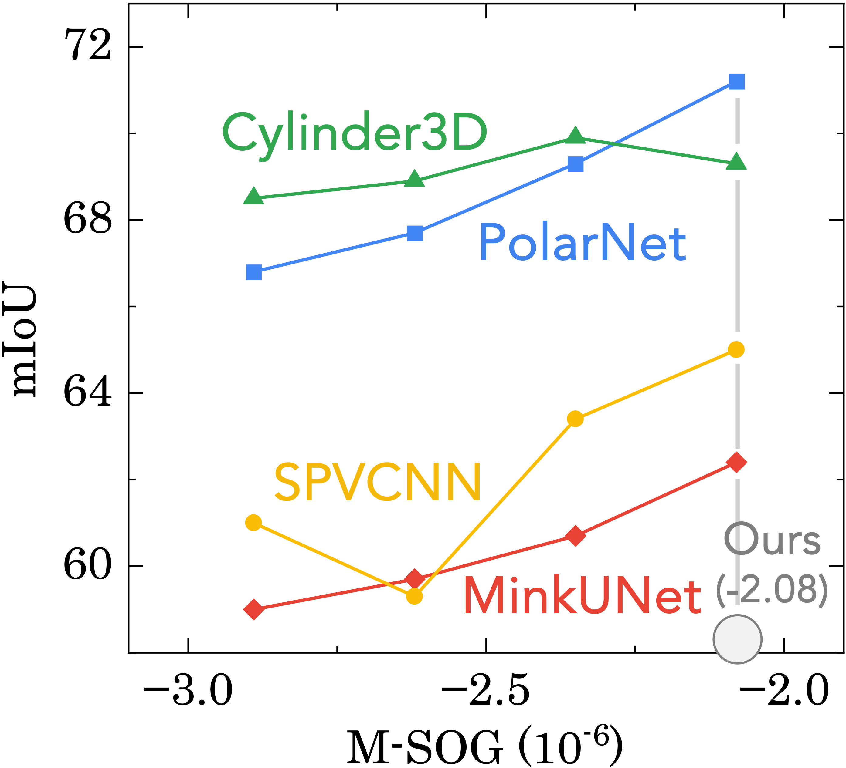
(a) Clean (Plane)

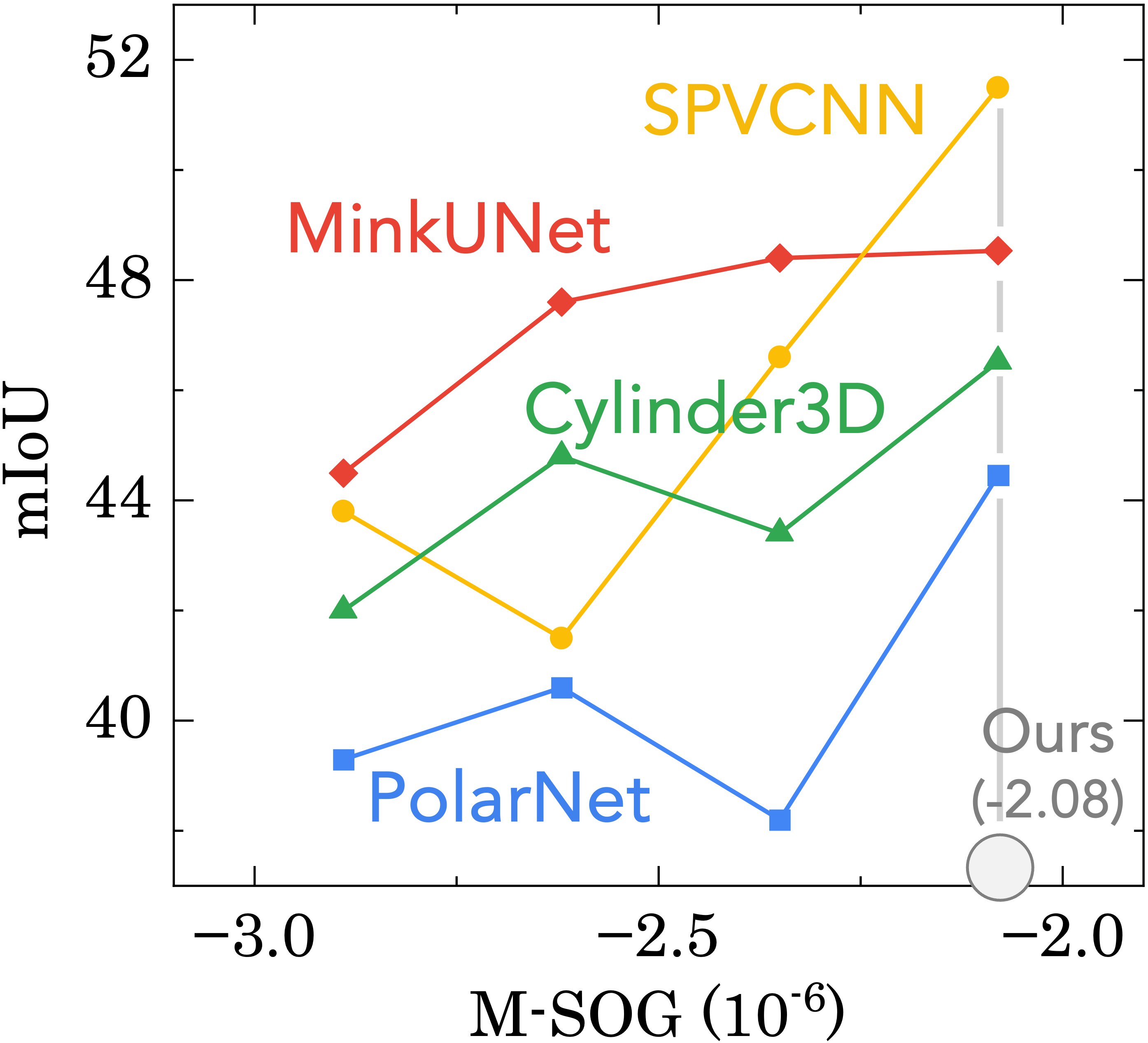
(b) Corruptions (Plane)

Figure 6: Optimization results with constrained placement options. From left to right are Trapezoid, Line, Square, and our optimized placement on 2D plane.

Optimizing under Constrained Placement Options. In automotive design practice, placing LiDARs at different heights on the roof might affect aesthetics and aerodynamics. Therefore, we investigate the effect of our optimization algorithm in the presence of constraints, by limiting the LiDARs to the same height and considering only 2D placements. We fix the height of all LiDARs to find the optimal placement on the horizontal plane of the vehicle roof. We use the line, square, and trapezoid placements in Fig. 4 for comparison. Experimental results in Figs. 6(a) and 6(b) show that our optimized placement generally outperforms baseline placement at the same LiDAR height on both clean and corruption settings.

5 Conclusion

In this work, we presented Place3D, a comprehensive and systematic LiDAR placement evaluation and optimization framework. We introduced the Surrogate Metric of Semantic Occupancy Grids (M-SOG) as a novel metric to assess the impact of various LiDAR placements. Building on this metric, we culminated an optimization approach for LiDAR configuration that significantly enhances detection and segmentation performance. We validate the effectiveness of our optimization approach through a multi-condition multi-LiDAR point cloud dataset and establish a comprehensive benchmark for evaluating both baseline and our optimized LiDAR placements on detection and segmentation in diverse conditions. Our optimized placements demonstrate superior robustness and perception capabilities, outperforming all baseline configurations. By shedding light on refining the robustness of LiDAR placements for both detection and segmentation tasks under adverse conditions, we anticipate that our work will pave the way for further advancements in this field.

Appendix

• 6. Place3D Dataset 6

  • 6.1 Statistics 6.1

  • 6.2 Data Collection 6.2

  • 6.3 Label Mappings 6.3

  • 6.4 Adverse Conditions 6.4

  • 6.5 License 6.5

• 7. Additional Implementation Detail 7

  • 7.1 LiDAR Placement 7.1

  • 7.2 Corruption Generation 7.2

  • 7.3 Hyperparameters 7.3

• 8. Additional Quantitative Result 8

  • 8.1 LiDAR Semantic Segmentation 8.1

  • 8.2 3D Object Detection 8.2

• 9. Additional Qualitative Result 9

  • 9.1 Clean Condition 9.1

  • 9.2 Adverse Conditions 9.2

• 10. Proofs 10

  • 10.1 Full Proof of Theorem 1 10.1

  • 10.2 Proof of Remark 1 10.2

• 11. Discussion 11

  • 11.1 Limitations 11.1

  • 11.2 Potential Societal Impact 11.2

• 12. Public Resources Used 12

6 Place3D Dataset

In this section, we present additional information on the statistics, features, and implementation details of the proposed Place3D dataset.

6.1 Statistics

Our dataset consists of a total of eleven LiDAR placements, in which seven baselines are inspired by existing self-driving configurations from autonomous vehicle companies and four LiDAR placements are obtained by optimization. Each LiDAR placement contains four LiDAR sensors. For each LiDAR configuration, the sub-dataset consists of 13,600 frames of samples, comprising 11,200 samples for training and 2,400 samples for validation, following the split ratio used in nuScenes [13]. We combined every 40 frames of samples into one scene, with a time interval of 0.5 seconds between each frame sample.

Table 6: Comparisons between Place3D and popular driving perception datasets with supports for the LiDAR semantic segmentation and 3D object detection tasks. Notably, the classes reported below represent those used for training and testing, with the actual number potentially exceeding what is shown.

	nuScenes	Waymo	SemKITTI	Place3D
Detection Classes	$10$	$2$	$3$	$3$
Segmentation Classes	$16$	$23$	$19$	$21$
# of 3D Boxes	$12$M	$1.4$M	$80$K	$71$K
Points Per Frame	$34$K	$177$K	$120$K	$16$K
# of LiDAR Channels	$1\times 32$	$1\times 64$	$1\times 64$	$4\times 16$
Vertical FOV	$[-30.0,10.0]$	$[-17.6,2.4]$	$[-24.8,2.0]$	$[-24.8,2.0]$
Placement Strategy	Single	Single	Single	Multiple
Adverse Conditions	No	No	No	Yes

Table 7: The attributes of the semantic LiDAR sensors used for acquiring the data.

Attribute	Value	Attribute	Value
Channels	$16$	Upper FOV	$2.0$ degrees
Range	$100.0$ meters	Lower FOV	$-24.8$ degrees
Points Per Second	5,000 $\times$ channels	Horizontal FOV	$360.0$ degrees
Rotation Frequency	$20.0$ Hz	Sensor Tick	$0.5$ second

6.2 Data Collection

6.2.1 Simulator Setup.

We choose four maps (Towns 1, 3, 4, and 6, c.f. Fig. 7) in CARLA v0.9.10 to collect point cloud data and generate ground truth information. For each map, we manually set 6 ego-vehicle routes to cover all roads with no roads overlapped. The frequency of the simulation is set to 20 Hz.

6.2.2 LiDAR Setup.

LiDAR point cloud data is collected every 0.5 simulator seconds utilizing the Semantic LIDAR sensor in CARLA. The attributes of Semantic LIDAR sensor are listed in Tab. 7. Notably, we utilize LiDARs with relatively low resolution to increase the challenge in object detection and semantic segmentation, leading to lower scores than those on the nuScenes [13] leaderboard. This is based on the observation that LiDAR point clouds become sparse when detecting distant objects and the use of multiple LiDARs is specifically to enhance the perception of sparse point clouds at long distances in practical applications. Our experiments with low-resolution LiDARs allow for a more evident assessment of the impact of LiDAR placements on the perception of sparse point clouds.

(a) Town 1

(b) Town 3

(c) Town 4

(d) Town 6

Figure 7: The maps used to collect Place3D data in CARLA v0.9.10.

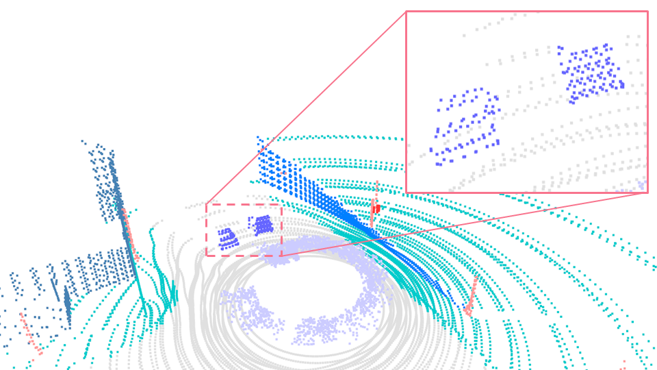
(a) fog

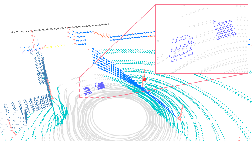
(b) wet ground

(c) snow

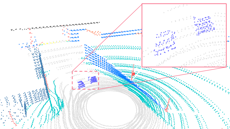
(d) motion blur

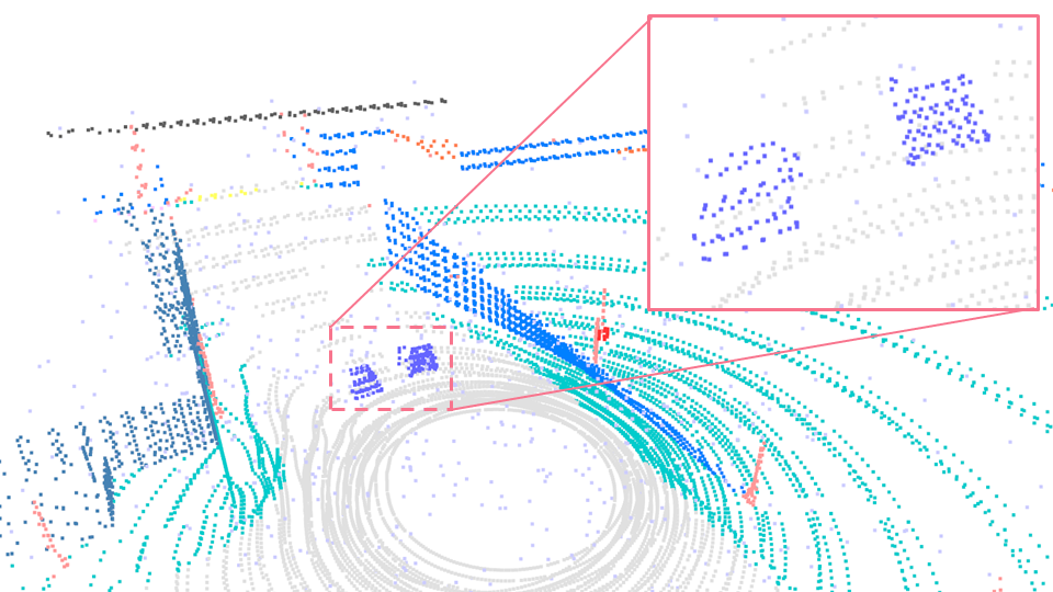
(e) crosstalk

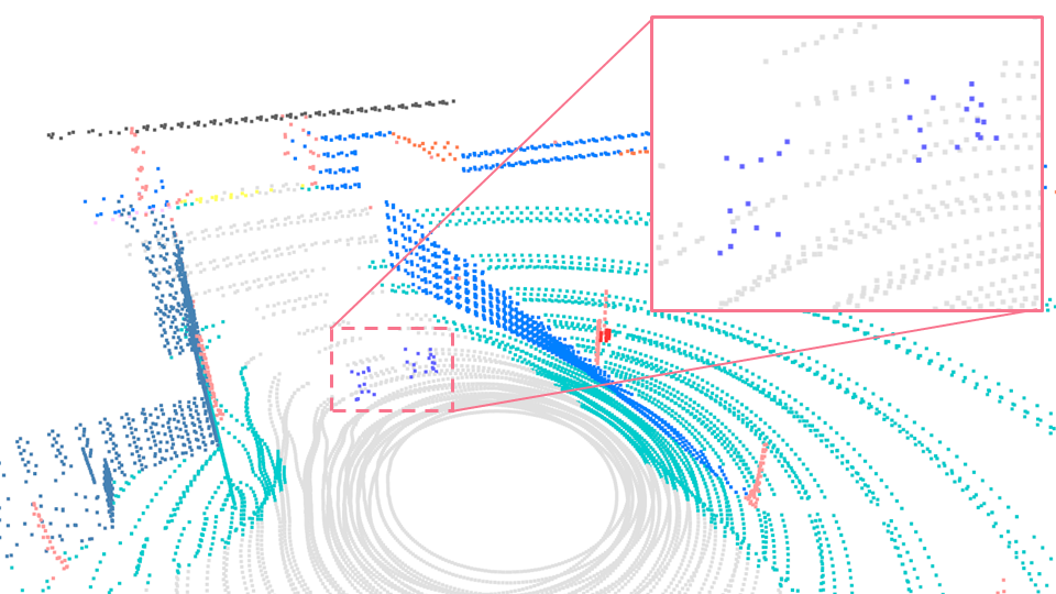
(f) incomplete echo

Figure 8: Visual examples of LiDAR point clouds under adverse conditions in Place3D.

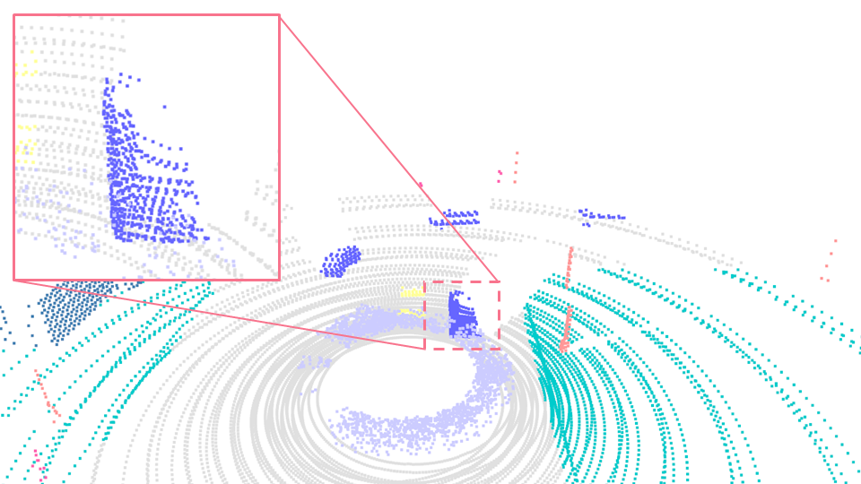
(a) fog

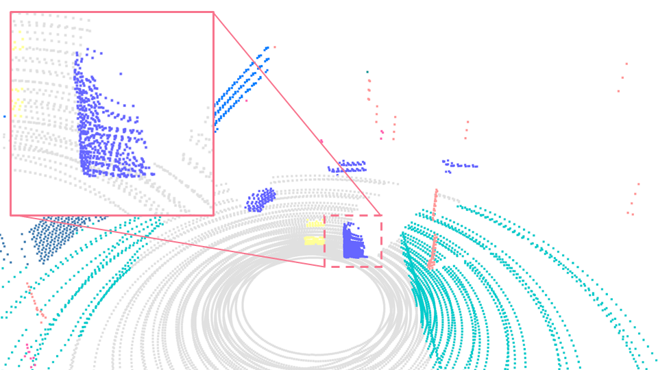
(b) wet ground

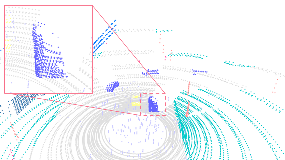
(c) snow

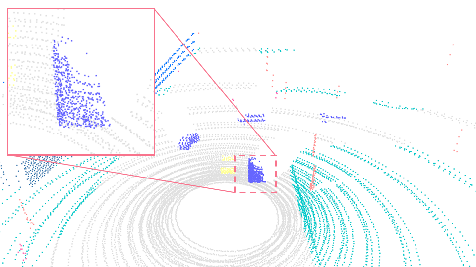
(d) motion blur

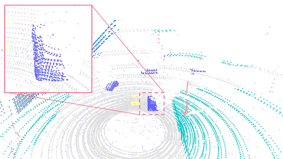
(e) crosstalk

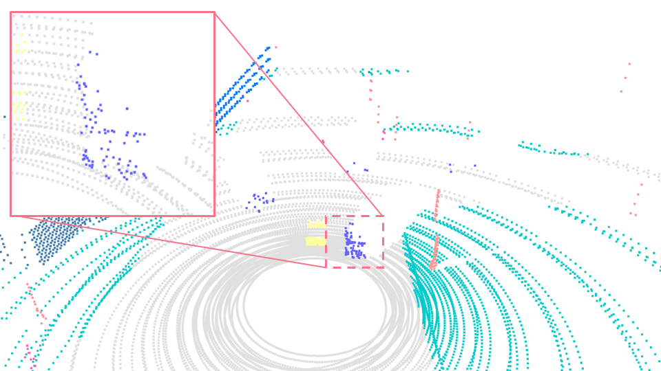
(f) incomplete echo

Figure 9: Visual examples of LiDAR point clouds under adverse conditions in Place3D.

Table 8: Summary of the semantic categories defined in the Place3D dataset.

Class	ID	Description
Building $\blacksquare$	1	Houses, skyscrapers, etc., and the manmade elements attached to them, such as scaffolding, awning, and ladders.
Fence $\blacksquare$	2	Barriers, railing, and other upright structures that are made by wood or wire assemblies and enclose an area of ground.
Other $\blacksquare$	3	Everything that does not belong to any other category.
Pedestrian $\blacksquare$	4	Humans that walk, ride, or drive any kind of vehicle or mobility system, such as bicycles, scooters, skateboards, wheelchairs, etc.
Pole $\blacksquare$	5	Small mainly vertically oriented poles, such as sign poles and traffic light poles.
Road Line $\blacksquare$	6	Markings on the road.
Road $\blacksquare$	7	Part of ground on which vehicles usually drive.
Sidewalk $\blacksquare$	8	Part of ground designated for pedestrians or cyclists, which is delimited from the road by some obstacle, such as curbs or poles.
Vegetation $\blacksquare$	9	Trees, hedges, and all other types of vertical vegetation.
Vehicle $\blacksquare$	10	Cars, vans, trucks, motorcycles, bikes, buses, and trains.
Wall $\blacksquare$	11	Individual standing walls that are not part of a building.
Traffic Sign $\blacksquare$	12	Signs installed by the city authority and are usually for traffic regulation.
Ground $\blacksquare$	13	Horizontal ground-level structures that do not match any other category.
Bridge $\blacksquare$	14	The structure of the bridge.
Rail Track $\blacksquare$	15	All types of rail tracks that are not driveable by cars.
Guard Rail $\blacksquare$	16	All types of guard rails and crash barriers.
Traffic Light $\blacksquare$	17	Traffic light boxes without their poles.
Static $\blacksquare$	18	Elements in the scene and props that are immovable, such fire hydrants, fixed benches, fountains, bus stops, etc.
Dynamic $\blacksquare$	19	Elements whose position is susceptible to change over time, such as movable trash bins, buggies, bags, wheelchairs, animals, etc.
Water $\blacksquare$	20	Horizontal water surfaces, such as lakes, sea, and rivers.
Terrain $\blacksquare$	21	Grass, ground-level vegetation, soil, and sand.

6.3 Label Mappings

6.3.1 LiDAR Semantic Segmentation.

There are a total of 21 semantic labels in our LiDAR semantic segmentation dataset, which are ¹Building, ²Fence, ³Other, ⁴Pedestrian, ⁵Pole, ⁶Road Line, ⁷Road, ⁸Sidewalk, ⁹Vegetation, ¹⁰Vehicle, ¹¹Wall, ¹²Traffic Sign, ¹³Ground, ¹⁴Bridge, ¹⁵Rail Track, ¹⁶Guard Rail, ¹⁷Traffic Light, ¹⁸Static, ¹⁹Dynamic, ²⁰Water, and ²¹Terrain. Tab. 8 presents the detailed definition of each semantic class in the Place3D dataset. Additionally, we include a Unlabeled tag to denote elements that have not been categorized.

6.3.2 3D Object Detection.

We set 3 types of common objects in the traffic scene for the 3D object detection tasks, i.e., ¹Car, ²Bicyclist, and ³Pedestrian, following the same configuration as KITTI [29].

6.4 Adverse Conditions

As shown in Fig. 8 and Fig. 9, the adverse conditions in the Place3D dataset can be categorized into three distinct groups: 1) Severe weather conditions, including “fog”, which causes back-scattering and attenuation of LiDAR points due to water particles in the air; “snow”, where snow particles intersect with laser beams, affecting the beam’s reflection and causing potential occlusions; and “wet ground”, where laser pulses lose energy upon hitting wet surfaces, leading to attenuated echoes. 2) External disturbances like “motion blur”, which resulted from vehicle movement that causes blurring in the data, especially on bumpy surfaces or during rapid turns. 3) Internal sensor failure, such as “crosstalk”, where the light impulses from multiple sensors interfere with each other, creating noisy points; as well as “incomplete echo”, where dark-colored objects result in incomplete LiDAR readings.

6.5 License

The Place3D dataset is released under the CC BY-NC-SA 4.0 license.

7 Additional Implementation Detail

In this section, we present additional implementation details to facilitate the reproduction of this work.

7.1 LiDAR Placement

We adopt five commonly employed heuristic LiDAR placements, which have been adopted by several leading autonomous driving companies, as our baseline. We create another two baseline placements by adjusting the rolling angles of LiDAR sensors. We obtain two placements in optimization and two placements in the ablation study. All configurations are presented in Tab. 9.

Table 9: The configuration coordinates of different LiDAR placement strategies in this work with respect to their ego-vehicle coordinate frames from four LiDAR sensors.

Placement	LiDAR #1				LiDAR #2				LiDAR #3				LiDAR #4
	$x$	$y$	$z$	roll	$x$	$y$	$z$	roll	$x$	$y$	$z$	roll	$x$	$y$	$z$	roll
Center	0.0	0.0	2.2	0.0	0.0	0.0	2.4	0.0	0.0	0.0	2.6	0.0	0.0	0.0	2.8	0.0
Line	0.0	-0.6	2.2	0.0	0.0	-0.4	2.2	0.0	0.0	0.4	2.2	0.0	0.0	0.6	2.2	0.0
Pyramid	-0.2	-0.6	2.2	0.0	0.4	0.0	2.4	0.0	-0.2	0.0	2.6	0.0	-0.2	0.6	2.2	0.0
Square	-0.5	0.5	2.2	0.0	-0.5	-0.5	2.2	0.0	0.5	0.5	2.2	0.0	0.5	-0.5	2.2	0.0
Trapezoid	-0.4	0.2	2.2	0.0	-0.4	-0.2	2.2	0.0	0.2	0.5	2.2	0.0	0.2	-0.5	2.2	0.0
Line-roll	0.0	-0.6	2.2	-0.3	0.0	-0.4	2.2	0.0	0.0	0.4	2.2	0.0	0.0	0.6	2.2	-0.3
Pyramid-roll	-0.2	-0.6	2.2	-0.3	0.4	0.0	2.4	0.0	-0.2	0.0	2.6	0.0	-0.2	0.6	2.2	-0.3
Ours-det	0.5	0.5	2.5	-0.3	-0.4	0.1	2.6	-0.2	0.0	0.0	2.8	0.0	-0.1	-0.5	2.7	0.0
Ours-seg	0.0	0.5	2.6	-0.3	0.6	0.3	2.8	0.0	0.4	0.0	2.5	0.0	0.1	-0.6	2.8	0.2
Corruption	0.4	0.5	2.6	-0.3	0.5	-0.4	2.7	0.0	-0.4	-0.3	2.7	0.1	-0.3	0.5	2.7	0.0
2D-plane	0.6	0.6	2.2	0.0	0.5	-0.4	2.2	0.0	-0.5	-0.6	2.2	0.0	-0.6	0.3	2.2	0.0

7.2 Corruption Generation

In this work, we adopt the public implementations from Robo3D [46] to generate corrupted point clouds. We follow the default configuration of generating nuScenes-C to construct the adverse condition sets in Place3D. Specifically, for “fog” generation, the attenuation coefficient is randomly sampled from $[0,0.005,0.01,0.02,0.03,0.06]$ and the back-scattering coefficient is set as $0.05$. For “wet ground” generation, the water height is set as $1.0$ millimeter. For “snow” generation, the value of snowfall rate parameter is set to $1.0$. For “motion blur” generation, the jittering noise level is set as $0.30$. For “crosstalk” generation, the disturb noise parameter is set to $0.07$. For “incomplete echo” generation, the attenuation parameter is set to $0.85$.

7.3 Hyperparameters

In this work, we build the LiDAR placement benchmark using the MMDetection3D codebase [23]. Unless otherwise specified, we follow the conventional setups in MMDetection3D when training and evaluating the LiDAR semantic segmentation and 3D object detection models.

The detailed training configurations of the four LiDAR semantic segmentation models, i.e., MinkUNet [21], SPVCNN [78], PolarNet [99], and Cylinder3D [105], are presented in Tab. 10. The detailed training configurations of the four 3D object detection models, i.e., PointPillars [50], CenterPoint [95], BEVFusion-L [58], and FSTR [97], are presented in Tab. 11.

All LiDAR semantic segmentation models are trained and tested on eight NVIDIA A100 SXM4 80GB GPUs. All 3D object detection models are trained and tested on four NVIDIA RTX 6000 Ada 48GB GPUs. The models are evaluated on the validation sets. We do not include any type of test time augmentation or model ensembling when evaluating the models.

Table 10: The training and optimization configurations of the four LiDAR semantic segmentation models [21, 78, 99, 105] used in our Place3D benchmark.

Hyperparameter	MinkUNet	SPVCNN	PolarNet	Cylinder3D
Batch Size	8 $\times$ b2	8 $\times$ b2	8 $\times$ b2	8 $\times$ b2
Epochs	50	50	50	50
Optimizer	AdamW	AdamW	AdamW	AdamW
Learning Rate	8.0$e-$3	8.0$e-$3	8.0$e-$3	8.0$e-$3
Weight Decay	0.01	0.01	0.01	0.01
Epsilon	1.0$e-$6	1.0$e-$6	1.0$e-$6	1.0$e-$6

Table 11: The training and optimization configurations of the four 3D object detection models [50, 95, 58, 97] used in our Place3D benchmark.

Hyperparameter	PointPillars	CenterPoint	BEVFusion-L	FSTR
Batch Size	4 $\times$ b4	4 $\times$ b4	4 $\times$ b4	4 $\times$ b4
Epochs	24	20	20	20
Optimizer	AdamW	AdamW	AdamW	AdamW
Learning Rate	1.0$e-$3	1.0$e-$4	1.0$e-$4	1.0$e-$4
Weight Decay	0.01	0.01	0.01	0.01
Epsilon	1.0$e-$6	1.0$e-$6	1.0$e-$6	1.0$e-$6

8 Additional Quantitative Result

In this section, we provide additional quantitative results, such as the class-wise LiDAR semantic segmentation results, to better support the findings and conclusions drawn in the main body of this paper.

Table 12: The per-class LiDAR semantic segmentation results of MinkUNet [21], SPVCNN [78], PolarNet [99], and Cylinder3D [105], under different LiDAR placement strategies. All mIoU ($\uparrow$) and class-wise IoU ($\uparrow$) scores are given in percentage (%).

Method	mIoU	$\blacksquare$ building	$\blacksquare$ fence	$\blacksquare$ other	$\blacksquare$ pedestrian	$\blacksquare$ pole	$\blacksquare$ road line	$\blacksquare$ road	$\blacksquare$ sidewalk	$\blacksquare$ vegetation	$\blacksquare$ vehicle	$\blacksquare$ wall	$\blacksquare$ traffic sign	$\blacksquare$ ground	$\blacksquare$ bridge	$\blacksquare$ rail track	$\blacksquare$ guard rail	$\blacksquare$ traffic light	$\blacksquare$ static	$\blacksquare$ dynamic	$\blacksquare$ water	$\blacksquare$ terrain
$\bullet$ Placement: Center
Mink	$65.7$	87.2	60.7	61.3	75.8	67.5	1.8	95.1	70.9	86.7	95.1	86.4	55.5	65.8	58.0	0.0	82.5	72.4	64.0	70.9	60.5	61.9
SPV	$67.1$	87.8	63.3	63.9	74.1	67.5	4.9	95.5	69.0	86.6	94.6	87.6	54.3	50.1	83.6	0.2	84.4	74.0	65.8	73.1	65.6	63.8
Polar	$71.0$	89.2	68.9	66.9	77.0	83.1	10.5	95.3	83.0	84.3	94.8	88.3	60.9	75.6	40.2	35.7	84.6	78.9	62.3	75.8	60.8	75.6
Cy3D	$72.7$	90.7	67.6	71.5	79.4	80.8	11.4	96.1	74.6	86.8	94.8	90.4	56.0	63.1	85.4	30.2	92.9	84.4	66.0	74.3	66.3	64.0
Avg	$69.1$	88.7	65.1	65.9	76.6	74.7	7.2	95.5	74.4	86.1	94.8	88.2	56.7	63.7	66.8	16.5	86.1	77.4	64.5	73.5	63.3	66.3
$\bullet$ Placement: Line
Mink	$59.7$	84.1	48.2	61.9	73.1	69.4	2.0	95.0	72.6	80.5	93.7	81.7	42.5	60.0	40.1	0.0	79.4	37.7	53.5	59.2	57.7	61.8
SPV	$59.3$	84.7	50.6	64.9	74.7	69.1	4.5	94.9	62.1	81.0	94.0	83.7	48.6	40.5	76.4	0.0	80.1	40.0	56.8	58.6	33.0	47.2
Polar	$67.7$	89.6	65.1	59.6	79.6	83.9	2.2	95.1	81.1	82.8	94.4	87.7	49.1	72.6	69.4	16.5	81.1	54.7	59.6	72.8	53.7	71.0
Cy3D	$68.9$	87.3	63.3	74.1	70.5	80.4	14.6	96.1	70.9	84.1	96.1	86.7	52.1	57.4	80.9	19.1	87.6	71.9	64.0	68.9	51.7	60.2
Avg	$63.9$	86.4	56.8	65.1	74.5	75.7	5.8	95.3	71.7	82.1	94.6	85.0	48.1	57.6	66.7	8.9	82.1	51.1	58.5	64.9	49.0	60.1
$\bullet$ Placement: Pyramid
Mink	$62.7$	87.4	57.6	64.9	76.5	73.5	2.4	94.5	65.1	82.3	93.7	85.2	49.6	47.7	57.1	0.0	83.5	65.3	59.1	60.9	54.2	55.6
SPV	$67.6$	88.2	60.7	70.2	78.3	72.6	9.7	95.5	74.6	81.7	92.1	87.4	55.5	54.5	86.4	0.0	81.8	68.1	64.5	69.2	62.6	65.9
Polar	$67.7$	90.3	64.7	55.1	78.6	84.9	6.2	95.2	83.3	84.7	94.8	87.4	57.8	74.8	32.2	28.5	85.8	45.6	58.9	78.2	60.9	74.4
Cy3D	$68.4$	87.4	67.8	70.5	81.2	82.0	12.7	95.2	67.4	84.3	96.4	86.0	56.4	54.2	53.5	20.9	87.1	81.0	67.3	71.3	57.3	55.6
Avg	$66.6$	88.3	62.7	65.2	78.7	78.3	7.8	95.1	72.6	83.3	94.3	86.5	54.8	57.8	57.3	12.4	84.6	65.0	62.5	69.9	58.8	62.9
$\bullet$ Placement: Square
Mink	$60.7$	85.3	51.1	63.7	75.1	70.6	3.2	95.5	64.7	81.6	95.2	83.7	46.2	44.8	63.9	0.0	79.2	46.3	54.7	57.6	59.4	52.0
SPV	$63.4$	85.9	54.3	69.5	75.8	70.5	6.0	95.4	68.9	82.1	95.5	84.6	50.1	53.7	82.8	0.0	80.2	40.7	59.2	63.0	58.4	54.5
Polar	$69.3$	89.9	64.7	57.2	79.1	84.0	3.5	95.3	82.4	83.9	95.1	88.9	50.0	75.6	75.4	20.2	86.0	58.2	58.8	75.8	58.2	73.8
Cy3D	$69.9$	88.7	63.6	75.1	80.5	81.5	13.8	96.2	76.9	84.9	97.2	88.0	55.1	65.9	51.8	22.3	90.9	72.5	67.5	74.9	55.4	65.2
Avg	$65.8$	87.5	58.4	66.4	77.6	76.7	6.6	95.6	73.2	83.1	95.8	86.3	50.4	60.0	68.5	10.6	84.1	54.4	60.1	67.8	57.9	61.4
$\bullet$ Placement: Trapezoid
Mink	$59.0$	84.5	43.8	64.0	74.4	70.0	2.4	95.4	68.7	81.7	94.6	82.6	47.1	54.1	43.7	0.0	82.6	52.8	53.9	54.8	32.1	56.1
SPV	$61.0$	85.8	54.5	70.0	73.7	70.4	7.9	95.1	64.5	82.2	94.9	84.4	49.5	40.2	74.3	0.0	76.4	53.6	60.0	60.4	30.7	52.1
Polar	$66.8$	90.1	62.6	59.0	79.3	83.7	4.5	95.1	78.0	83.9	95.2	87.7	53.4	74.6	42.0	18.8	84.7	54.6	55.7	74.4	57.2	67.7
Cy3D	$68.5$	88.4	63.1	75.2	80.3	80.2	15.1	96.1	72.6	83.4	95.8	87.9	54.5	61.8	55.7	13.8	83.9	77.8	64.6	66.4	64.8	58.1
Avg	$63.8$	87.2	56.0	67.1	76.9	76.1	7.5	95.4	71.0	82.8	95.1	85.7	51.1	57.7	53.9	8.2	81.9	59.7	58.6	64.0	46.2	58.5
$\bullet$ Placement: Line-Roll
Mink	$58.5$	85.3	47.3	57.9	73.8	69.6	2.3	95.1	71.8	79.2	91.4	81.6	47.7	56.7	22.2	0.0	78.3	45.5	54.2	56.1	53.6	58.2
SPV	$60.6$	85.5	53.6	62.5	74.3	70.5	3.4	95.3	67.1	81.0	91.6	84.5	53.5	49.9	82.6	0.2	78.3	44.8	54.2	61.7	27.4	51.8
Polar	$67.2$	90.6	65.5	54.1	79.4	84.5	2.8	94.8	81.5	83.0	94.4	88.2	50.1	68.9	39.3	21.2	87.4	63.8	56.4	71.6	61.3	72.9
Cy3D	$69.8$	87.1	58.9	74.5	80.7	81.8	13.4	96.5	76.0	84.1	96.6	86.0	55.5	63.7	62.4	22.8	90.5	75.9	66.6	74.9	55.0	62.0
Avg	$64.0$	87.1	56.3	62.3	77.1	76.6	5.5	95.4	74.1	81.8	93.5	85.1	51.7	59.8	51.6	11.1	83.6	57.5	57.9	66.1	49.3	61.2
$\bullet$ Placement: Pyramid-Roll
Mink	$62.2$	87.5	52.2	63.5	76.1	73.7	2.1	94.3	63.3	81.7	94.9	84.1	55.0	43.5	50.4	0.0	81.0	64.6	61.5	59.3	62.0	55.5
SPV	$67.9$	88.5	61.2	69.5	78.4	73.6	7.4	95.1	72.2	83.9	94.4	87.6	58.2	55.7	87.9	0.0	83.3	65.0	66.2	68.7	64.7	64.6
Polar	$70.9$	90.8	67.0	61.0	79.1	84.7	5.1	95.1	82.1	85.0	95.5	88.4	64.0	73.3	50.1	24.7	89.3	73.6	61.7	75.4	68.4	73.8
Cy3D	$69.3$	87.8	60.2	69.0	81.0	80.9	12.0	95.1	65.1	85.3	96.3	88.3	53.5	57.6	82.8	32.7	88.5	77.0	65.9	70.2	57.0	48.1
Avg	$67.9$	88.5	61.2	69.5	78.4	73.6	7.4	95.1	72.2	83.9	94.4	87.6	58.2	55.7	87.9	0.0	83.3	65.0	66.2	68.7	64.7	64.6
$\bullet$ Placement: Ours
Mink	$66.5$	89.6	56.7	65.1	73.3	76.4	4.2	94.6	70.7	86.0	94.0	83.8	62.8	55.9	49.2	2.6	85.4	74.6	63.3	66.5	78.6	62.4
SPV	$68.3$	89.8	59.5	66.8	75.2	75.8	6.0	94.6	74.2	85.9	93.4	85.3	60.1	58.7	75.5	0.0	85.5	76.7	64.9	65.2	77.3	64.7
Polar	$76.7$	93.5	70.6	60.7	79.6	86.1	8.6	96.0	86.1	87.2	94.9	88.8	68.0	78.8	56.6	76.1	89.0	86.1	63.6	79.1	82.2	78.2
Cy3D	$73.0$	91.7	66.5	68.3	80.2	85.1	12.7	96.1	82.2	86.9	95.3	86.7	54.0	58.4	28.9	68.2	90.8	83.9	73.8	79.3	74.7	69.3
Avg	$71.1$	91.2	63.3	65.2	77.1	80.9	7.9	95.3	78.3	86.5	94.4	86.2	61.2	63.0	52.6	36.7	87.7	80.3	66.4	72.5	78.2	68.7

Table 13: Benchmark results of LiDAR semantic segmentation under clean and adverse conditions. For each placement, we report the mIoU ($\uparrow$), mAcc ($\uparrow$), and ECE ($\downarrow$) scores for models under the clean condition, and mIoU ($\uparrow$) scores for models under adverse conditions. The mIoU and mAcc scores are given in percentage ($\%$).

Method	Clean			Adverse
	mIoU	mAcc	ECE	Fog	Wet	Snow	Blur	Cross	Echo	Avg
$\bullet$ Placement: Center
MinkUNet [21]	$65.7$	$72.4$	$0.041$	55.9	63.8	25.1	35.8	24.7	64.5	45.0
SPVCNN [78]	$67.1$	$74.4$	$0.034$	39.3	66.6	35.6	35.6	19.5	66.8	43.9
PolarNet [99]	$71.0$	$76.0$	$0.033$	43.1	59.2	11.4	36.1	23.1	69.4	40.4
Cylinder3D [105]	$72.7$	$79.2$	$0.041$	55.6	64.4	16.7	37.6	36.9	71.5	47.1
$\bullet$ Placement: Line
MinkUNet [21]	$59.7$	$67.7$	$0.037$	51.7	60.2	35.5	52.0	27.1	59.2	47.6
SPVCNN [78]	$59.3$	$66.7$	$0.068$	42.8	57.9	31.3	46.1	13.6	57.1	41.5
PolarNet [99]	$67.7$	$74.1$	$0.034$	43.1	61.6	4.4	48.4	18.9	67.3	40.6
Cylinder3D [105]	$68.9$	$76.3$	$0.045$	55.5	66.4	4.7	39.4	34.3	68.3	44.8
$\bullet$ Placement: Pyramid
MinkUNet [21]	$62.7$	$70.6$	$0.072$	52.9	60.3	25.2	50.7	17.3	60.2	44.4
SPVCNN [78]	$67.6$	$74.0$	$0.037$	48.6	66.6	30.2	55.1	14.8	65.9	46.9
PolarNet [99]	$67.7$	$73.0$	$0.032$	34.3	61.0	2.3	49.1	9.6	66.9	37.2
Cylinder3D [105]	$68.4$	$76.0$	$0.093$	51.0	52.2	5.0	42.5	26.6	60.9	39.7
$\bullet$ Placement: Square
MinkUNet [21]	$60.7$	$68.4$	$0.043$	55.6	61.9	33.5	51.5	26.5	61.2	48.4
SPVCNN [78]	$63.4$	$70.2$	$0.031$	40.7	64.3	38.3	53.9	18.6	63.7	46.6
PolarNet [99]	$69.3$	$74.7$	$0.033$	39.9	50.0	6.1	49.1	15.1	68.8	38.2
Cylinder3D [105]	$69.9$	$76.7$	$0.044$	52.0	55.6	2.7	44.2	37.1	68.7	43.4
$\bullet$ Placement: Trapezoid
MinkUNet [21]	$59.0$	$66.2$	$0.040$	49.7	60.4	27.6	51.7	18.4	59.3	44.5
SPVCNN [78]	$61.0$	$68.8$	$0.044$	40.9	61.3	33.6	49.1	16.9	60.7	43.8
PolarNet [99]	$66.8$	$72.3$	$0.034$	37.5	65.3	2.8	46.7	15.4	67.8	39.3
Cylinder3D [105]	$68.5$	$75.4$	$0.057$	52.1	64.6	3.1	36.7	30.0	65.6	42.0
$\bullet$ Placement: Line-Roll
MinkUNet [21]	$58.5$	$66.4$	$0.047$	48.6	59.2	26.9	50.4	21.2	58.0	44.1
SPVCNN [78]	$60.6$	$68.0$	$0.034$	42.2	62.0	27.0	49.9	16.5	61.0	43.1
PolarNet [99]	$67.2$	$72.8$	$0.037$	38.2	62.9	2.2	46.3	14.2	65.4	38.2
Cylinder3D [105]	$69.8$	$77.0$	$0.048$	49.7	65.4	2.6	37.4	27.3	67.8	41.7
$\bullet$ Placement: Pyramid-Roll
MinkUNet [21]	$62.2$	$69.6$	$0.051$	52.2	60.9	26.6	52.5	19.3	60.8	45.4
SPVCNN [78]	$67.9$	$74.2$	$0.033$	47.2	67.1	31.6	56.5	13.7	66.7	47.1
PolarNet [99]	$70.9$	$75.9$	$0.035$	36.3	49.1	2.3	51.4	13.3	68.6	36.8
Cylinder3D [105]	$69.3$	$77.0$	$0.048$	50.7	67.9	2.1	44.1	31.9	70.0	44.5
$\bullet$ Placement: Ours
MinkUNet [21]	$66.5$	$73.2$	$0.031$	59.5	66.6	17.6	56.7	24.5	66.9	48.6
SPVCNN [78]	$68.3$	$74.6$	$0.034$	59.1	66.7	24.0	56.0	18.7	66.9	48.6
PolarNet [99]	$76.7$	$81.5$	$0.033$	57.3	65.8	2.8	55.0	27.3	76.1	47.4
Cylinder3D [105]	$73.0$	$78.9$	$0.037$	57.6	67.2	5.9	48.7	41.0	63.3	47.3

Table 14: Benchmark results of 3D object detection under clean and adverse conditions. For each placement, we report the mAP ($\uparrow$) scores of three classes (car, pedestrian, and bicyclist) for models under the clean condition, and mAP ($\uparrow$) scores of car for models under adverse conditions. The mAP scores are given in percentage ($\%$).

Method	Clean			Adverse
	Car	Ped	Bicy	Fog	Wet	Snow	Blur	Cross	Echo	Avg
$\bullet$ Placement: Center
PointPillars [50]	$46.5$	$19.4$	$27.1$	17.1	36.3	37.4	27.1	25.7	26.2	28.3
CenterPoint [95]	$55.8$	$28.7$	$28.8$	23.2	47.3	18.9	27.3	31.6	22.3	28.4
BEVFusion-L [58]	$52.5$	$31.9$	$32.2$	19.2	36.8	27.0	12.8	8.3	20.9	20.8
FSTR [97]	$55.3$	$27.7$	$29.3$	23.8	44.1	30.7	25.4	25.0	25.9	29.2
$\bullet$ Placement: Line
PointPillars [50]	$43.4$	$22.0$	$27.7$	15.1	39.6	33.6	27.1	16.9	25.2	26.3
CenterPoint [95]	$54.0$	$34.2$	$37.7$	20.2	49.2	22.8	9.7	12.0	21.5	22.6
BEVFusion-L [58]	$49.3$	$29.0$	$29.5$	18.6	38.0	12.2	23.6	17.2	21.6	21.9
FSTR [97]	$51.9$	$30.2$	$33.0$	22.7	45.4	27.0	23.9	20.1	27.0	27.7
$\bullet$ Placement: Pyramid
PointPillars [50]	$46.1$	$24.4$	$29.0$	17.2	38.7	36.1	29.2	26.3	25.8	28.9
CenterPoint [95]	$55.9$	$37.4$	$35.6$	26.0	49.6	21.1	28.6	24.9	25.9	29.4
BEVFusion-L [58]	$51.0$	$21.7$	$27.9$	20.8	38.1	15.0	29.1	23.7	21.6	24.7
FSTR [97]	$55.7$	$29.4$	$33.8$	25.8	44.8	24.0	33.4	28.5	28.7	30.9
$\bullet$ Placement: Square
PointPillars [50]	$43.8$	$20.8$	$27.1$	17.2	40.0	32.5	26.1	22.3	25.7	27.3
CenterPoint [95]	$54.0$	$35.5$	$34.1$	23.4	50.2	19.2	13.0	14.0	24.6	24.1
BEVFusion-L [58]	$49.2$	$27.0$	$26.7$	20.7	39.4	7.3	23.6	20.1	22.7	22.3
FSTR [97]	$52.8$	$30.3$	$31.3$	23.7	47.2	23.4	25.1	23.1	29.0	28.6
$\bullet$ Placement: Trapezoid
PointPillars [50]	$43.5$	$21.5$	$27.3$	16.0	40.0	31.3	25.9	18.6	24.9	26.1
CenterPoint [95]	$55.4$	$35.6$	$37.5$	22.1	51.7	14.6	15.3	11.6	23.9	23.2
BEVFusion-L [58]	$50.2$	$30.0$	$31.7$	19.2	39.2	19.8	26.9	27.2	22.6	25.8
FSTR [97]	$54.6$	$30.0$	$33.3$	22.9	46.9	26.0	26.5	23.4	26.5	28.7
$\bullet$ Placement: Line-Roll
PointPillars [50]	$44.6$	$21.3$	$27.0$	15.2	40.3	33.7	26.9	20.0	25.3	26.9
CenterPoint [95]	$55.2$	$32.7$	$37.2$	19.6	49.6	16.0	15.5	9.5	23.2	22.2
BEVFusion-L [58]	$50.8$	$29.4$	$29.5$	15.2	38.3	11.2	19.5	10.7	21.9	19.5
FSTR [97]	$53.5$	$29.8$	$32.4$	21.0	46.2	24.2	24.1	16.2	27.8	26.6
$\bullet$ Placement: Pyramid-Roll
PointPillars [50]	$46.1$	$23.6$	$27.9$	17.5	39.1	33.7	27.3	25.1	25.2	28.0
CenterPoint [95]	$56.2$	$36.5$	$35.9$	24.8	49.2	15.9	29.0	24.0	25.5	28.1
BEVFusion-L [58]	$50.7$	$22.7$	$28.2$	22.8	40.3	5.2	30.3	22.9	21.8	23.9
FSTR [97]	$55.5$	$29.9$	$32.0$	26.3	47.2	22.9	33.5	28.1	28.8	31.1
$\bullet$ Placement: Ours
PointPillars [50]	$46.8$	$24.9$	$27.2$	18.3	40.1	36.4	26.5	26.4	25.8	28.9
CenterPoint [95]	$57.1$	$34.4$	$37.3$	22.3	51.1	23.1	27.7	29.0	23.6	29.5
BEVFusion-L [58]	$53.0$	$28.7$	$29.5$	21.8	41.3	15.9	32.0	22.9	22.7	26.1
FSTR [97]	$56.6$	$31.9$	$34.1$	25.1	47.5	28.8	32.1	30.6	28.2	32.1

Table 15: Ablation study of LiDAR semantic segmentation under clean and adverse conditions. For each placement, we report the mIoU ($\uparrow$), mAcc ($\uparrow$), and ECE ($\downarrow$) scores for models under the clean condition, and mIoU ($\uparrow$) scores for models under adverse conditions. The mIoU and mAcc scores are given in percentage ($\%$).

Method	Clean			Adverse
	mIoU	mAcc	ECE	Fog	Wet	Snow	Blur	Cross	Echo	Avg
$\bullet$ Placement: Line
MinkUNet [21]	$59.7$	$67.7$	$0.037$	51.7	60.2	35.5	52.0	27.1	59.2	47.6
SPVCNN [78]	$59.3$	$66.7$	$0.068$	42.8	57.9	31.3	46.1	13.6	57.1	41.5
PolarNet [99]	$67.7$	$74.1$	$0.034$	43.1	61.6	4.4	48.4	18.9	67.3	40.6
Cylinder3D [105]	$68.9$	$76.3$	$0.045$	55.5	66.4	4.7	39.4	34.3	68.3	44.8
$\bullet$ Placement: Square
MinkUNet [21]	$60.7$	$68.4$	$0.043$	55.6	61.9	33.5	51.5	26.5	61.2	48.4
SPVCNN [78]	$63.4$	$70.2$	$0.031$	40.7	64.3	38.3	53.9	18.6	63.7	46.6
PolarNet [99]	$69.3$	$74.7$	$0.033$	39.9	50.0	6.1	49.1	15.1	68.8	38.2
Cylinder3D [105]	$69.9$	$76.7$	$0.044$	52.0	55.6	2.7	44.2	37.1	68.7	43.4
$\bullet$ Placement: Trapezoid
MinkUNet [21]	$59.0$	$66.2$	$0.040$	49.7	60.4	27.6	51.7	18.4	59.3	44.5
SPVCNN [78]	$61.0$	$68.8$	$0.044$	40.9	61.3	33.6	49.1	16.9	60.7	43.8
PolarNet [99]	$66.8$	$72.3$	$0.034$	37.5	65.3	2.8	46.7	15.4	67.8	39.3
Cylinder3D [105]	$68.5$	$75.4$	$0.057$	52.1	64.6	3.1	36.7	30.0	65.6	42.0
$\bullet$ Placement: Line-Roll
MinkUNet [21]	$58.5$	$66.4$	$0.047$	48.6	59.2	26.9	50.4	21.2	58.0	44.1
SPVCNN [78]	$60.6$	$68.0$	$0.034$	42.2	62.0	27.0	49.9	16.5	61.0	43.1
PolarNet [99]	$67.2$	$72.8$	$0.037$	38.2	62.9	2.2	46.3	14.2	65.4	38.2
Cylinder3D [105]	$69.8$	$77.0$	$0.048$	49.7	65.4	2.6	37.4	27.3	67.8	41.7
$\bullet$ Placement: 2D Plane
MinkUNet [21]	62.4	71.0	0.059	56.1	58.7	32.8	51.9	25.6	66.1	48.5
SPVCNN [78]	65.0	71.8	0.050	56.9	66.1	37.9	56.4	26.0	65.7	51.5
PolarNet [99]	71.2	76.4	0.046	52.8	64.4	5.0	51.7	23.0	69.8	44.5
Cylinder3D [105]	69.3	75.7	0.047	52.6	67.7	5.0	45.9	36.8	71.1	46.5
$\bullet$ Placement: Corruption Optimized
MinkUNet [21]	62.9	70.6	0.062	57.0	59.9	31.9	52.4	25.0	67.6	49.0
SPVCNN [78]	64.8	72.0	0.051	56.4	65.6	36.8	57.0	25.8	64.8	51.1
PolarNet [99]	73.9	79.3	0.037	60.7	66.4	5.6	54.4	34.8	76.8	49.8
Cylinder3D [105]	72.5	79.1	0.040	54.0	69.9	5.9	47.3	37.8	72.7	47.9
$\bullet$ Placement: Ours
MinkUNet [21]	$66.5$	$73.2$	$0.031$	59.5	66.6	17.6	56.7	24.5	66.9	48.6
SPVCNN [78]	$68.3$	$74.6$	$0.034$	59.1	66.7	24.0	56.0	18.7	66.9	48.6
PolarNet [99]	$76.7$	$81.5$	$0.033$	57.3	65.8	2.8	55.0	27.3	76.1	47.4
Cylinder3D [105]	$73.0$	$78.9$	$0.037$	57.6	67.2	5.9	48.7	41.0	63.3	47.3

8.1 LiDAR Semantic Segmentation

In this section, we provide the complete (i.e., the class-wise IoU scores) results for LiDAR semantic segmentation under different LiDAR placement strategies.

We showcase the per-class LiDAR semantic segmentation results of MinkUNet [21], SPVCNN [78], PolarNet [99], and Cylinder3D [105] in Tab. 12. The performance of these methods is evaluated under different LiDAR placement strategies. Different LiDAR placement strategies demonstrated varying propensities towards particular classes. For instance, Pyramid performs well for building, guard rail, and vegetation compared with other placements, possibly due to an increased vertical field of view that captures these taller or layered structures more effectively. Ours provides the generally best balance of performance across categories, with high scores in building, road, and vehicle suggesting an effective all-around coverage for various object types. The complete benchmark results of LiDAR semantic segmentation under clean and adverse conditions are presented in Tab. 13.

We showcase the complete results of the ablation study for semantic segmentation in Tab. 15. we first explore the performance of our optimization algorithm under placement constraints, specifically, standardize the elevation of LiDARs to analyze their optimal positioning on the vehicle’s roof’s horizontal plane. Our optimized placement 2D plane achieved better performance compared with line, square, and trapezoid configurations. Further, we optimize the placement for adverse conditions. While the observation suggests a trade-off in clean data compared with the Ours, the configuration optimized on corruption data (Corruption optimized) achieves a significantly higher performance in adverse conditions than both baselines in Tab. 13 and Ours, indicating that custom optimization strategies, tailored for challenging conditions, represent an effective methodology to enhance robust perception capabilities in adverse environments.

8.2 3D Object Detection

In this section, we present more experimental results for the 3D robustness evaluation of 3D object detection under adverse conditions. The performance of PointPillars[50], CenterPoint[95], BEVFusion-L[58], and FSTR[97] is evaluated under different LiDAR placement strategies in Tab. 14. Across all placements and conditions, there is a trend where all methods suffer a drop in performance in adverse conditions compared to clean conditions, highlighting the challenge that adverse conditions pose to 3D object detection. While some placements, like Pyramid and Square, appear to maintain relatively high performance under both clean and adverse conditions, the Ours placement has the highest average mAP under adverse conditions. In addition, certain placements exhibit relative strengths against specific types of corruption, which can inform the development of more resilient object detection systems for autonomous vehicles. For instance, Pyramid and Pyramid-Roll, appear to handle fog better than others, possibly due to a configuration that captures a more diverse set of angles which could mitigate the scattering effect of fog on LiDAR beams.

9 Additional Qualitative Result

In this section, we provide additional qualitative examples to help visually compare different conditions presented in this work.

9.1 Clean Condition

We showcase the qualitative results of the MinkUNet [21] model using our optimized LiDAR placement. As shown in Fig. 10, the depiction across the first four rows demonstrates a commendable performance of our LiDAR placement strategy during clean conditions. This is evidenced by the predominance of gray in the error maps, which indicate a high rate of correct predictions. Also, the fifth row presents a notable exception, illustrating a failure case. This particular scene exhibits a heightened complexity with a diverse array of objects and potential occlusions that challenge predictive accuracy. The qualitative results underscore the importance of continuous refinement of LiDAR placement to achieve better perception across a comprehensive spectrum of scenarios.

9.2 Adverse Conditions

In Fig. 11, we showcase the qualitative results of MinkUNet [21] under different adverse conditions utilizing our optimized LiDAR placement. The corruptions from top to bottom rows are “fog”, “wet ground”, “motion blur”, “crosstalk”, and “incomplete echo”. As can be seen, the LiDAR semantic segmentation model encounters extra difficulties when predicting under such scenarios. Erroneous predictions tend to appear in regions contaminated by different types of noises, such as airborne particles, disturbed laser reflections, and jittering scatters. It becomes apparent that enhancing the model’s robustness under these adverse conditions is crucial for the practical usage of driving perception systems. To achieve better robustness, we design suitable LiDAR placements that can mitigate the degradation caused by corruptions. As discussed in Tab. 13, Tab. 14, and Tab. 15, our placements can largely enhance the robustness of various models.

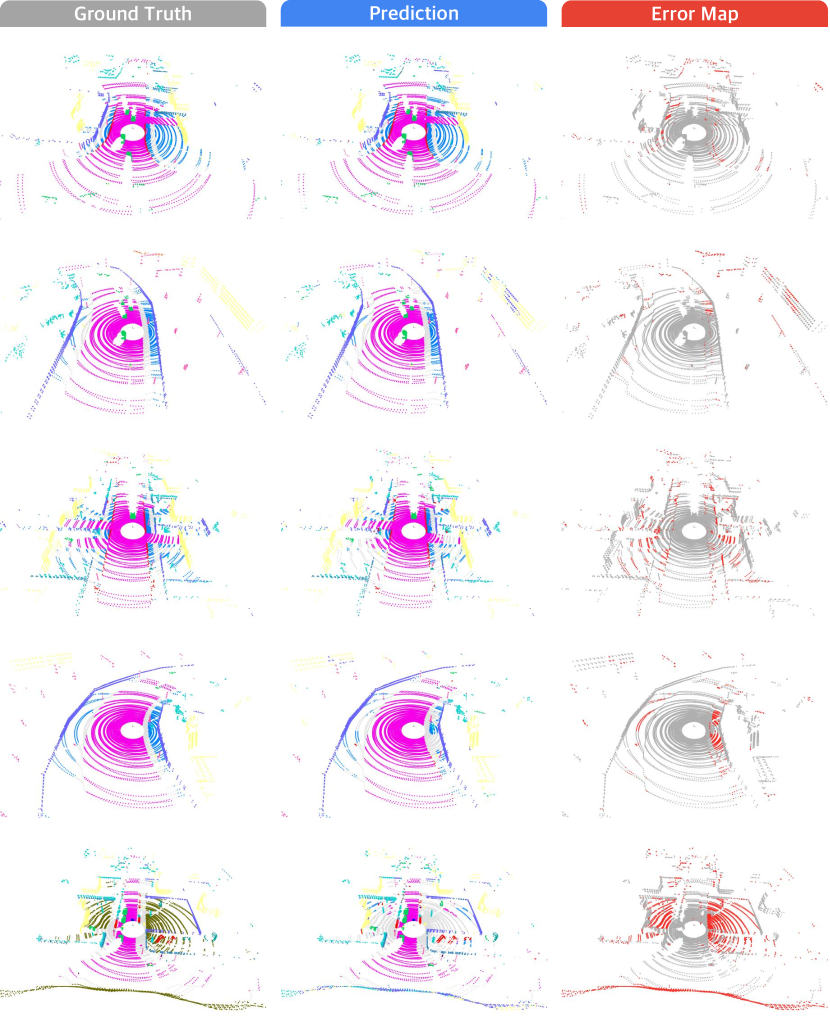
Figure 10: Qualitative assessments of the MinkUNet [21] model using our LiDAR placement strategy. The model is tested under the clean condition. The error maps show the correct and incorrect predictions in gray and red, respectively. Kindly refer to Tab. 8 for color maps. Best viewed in colors and zoomed-in for details.

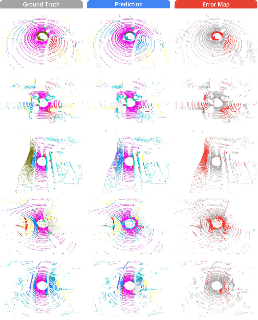
Figure 11: Qualitative assessments of the MinkUNet [21] model using our LiDAR placement strategy. The model is tested under adverse conditions. The error maps show the correct and incorrect predictions in gray and red, respectively. Kindly refer to Tab. 8 for color maps. Best viewed in colors and zoomed-in for details.

10 Proofs

In this section, we present the full proof of Theorem 1 to certify the global optimally regarding the solved local optima. Additionally, we present the proof of Remark 1 as a special case with bounded hyper-rectangle search space only given the Lipschitz constant of the objective function.

10.1 Full Proof of Theorem 1

Theorem 10.1 (Optimality Certification)

Given the continuous objective function $G:\mathbb{R}^{n}\to\mathbb{R}$ with Lipschitz constant $k_{G}$ w.r.t. input $\textbf{u}\in\mathcal{U}\subset\mathbb{R}^{n}$ under $\ell_{2}$ norm, suppose over a $\delta$-density Grids subset $S\subset\mathcal{U}$, the distance between the maximal and minimal of function $G$ over $S$ is upper-bounded by $C_{M}$, and the local optima is $\textbf{u}^{*}_{S}=\arg\min_{\textbf{u}\in S}G(x)$, the following optimality certification regarding $x\in\mathcal{U}$ holds that:

$$\|G(\textbf{u}^{*})-G(\textbf{u}^{*}_{S})\|_{2}~{}\leq~{}C_{M}+k_{G}\delta~{},$$ (16)

where $\textbf{u}^{*}$ is the global optima over $\mathcal{U}$.

Proof

Based on the sampling over subset $S\subset\mathcal{U}$ with $\ell_{2}$-norm density $\delta$, we have:

$$\forall\textbf{u}\in\mathcal{U},\min_{\textbf{u}_{S}\in S}\|\textbf{u}-\textbf{u}_{S}\|_{2}~{}\leq~{}\delta~{}.$$ (17)

From the continuous objective function $G:\mathbb{R}^{n}\to\mathbb{R}$ with Lipschitz constant $k_{G}$ w.r.t. input $\textbf{u}\in\mathcal{U}\subset\mathbb{R}^{n}$ under $\ell_{2}$ norm, it holds that:

$$\|G(\textbf{u}_{1})-G(\textbf{u}_{2})\|_{2}~{}\leq~{}k_{G}\|\textbf{u}_{1}-\textbf{u}_{2}\|_{2},~{}\forall\textbf{u}_{1},\textbf{u}_{2}\in\mathcal{U}~{}.$$ (18)

Since the distance between the maximal and minimal of function $G$ over $S$ is upper-bounded by $C_{M}$, we then have:

$$\|G(\textbf{u}_{1})-G(\textbf{u}_{2})\|_{2}~{}\leq~{}\|\max_{\textbf{u}\in S}G(\textbf{u})-\min_{\textbf{u}\in S}G(\textbf{u})\|_{2}~{}\leq~{}C_{M},\forall\textbf{u}_{1},\textbf{u}_{2}\in S~{}.$$ (19)

Then by absolute value inequality with $\textbf{u}_{S}\in S\subset\mathcal{U}~{}s.t.~{}\|\textbf{u}^{*}-\textbf{u}_{S}\|_{2}\leq\delta$ and combining all inequalities above, we have:

$$\|G(\textbf{u}^{*})-G(\textbf{u}^{*}_{S})\|_{2}~{}\leq~{} \|G(\textbf{u}^{*})-G(\textbf{u}_{S})\|_{2}+\|G(\textbf{u}^{*})-G(\textbf{u}_{S})\|_{2}$$ (20)

$$~{}\leq~{} k_{G}\|\textbf{u}^{*}-\textbf{u}_{S}\|_{2}+C_{M}$$ (21)

$$~{}\leq~{} k_{G}\delta+C_{M}~{},$$ (22)

which concludes the proof. $\blacksquare$

10.2 Proof of Remark 1

Remark 2

When $\mathcal{U}$ is a hyper-rectangle with the bounded $\ell_{2}$ norm of domain $U_{i}\in\mathbb{R}$ at each dimension $i$, with $i=1,2,\dots,n$, we remark Theorem 10.1 can hold in a more general way by only assuming that the Lipschitz constant $k_{G}$ of the objective function is given, where the following optimality certification regarding $x\in\mathcal{U}$ holds that:

$$\|G(\textbf{u}^{*})-G(\textbf{u}^{*}_{S})\|_{2}~{}\leq~{}k_{G}\sum_{i=1}^{n}{U_{i}}+k_{G}\delta~{}.$$ (23)

Proof

Similar to the proof of Thm 10.1, by the sampling over subset $S\subset\mathcal{U}$ with $\ell_{2}$-norm density $\delta$, we have:

$$\forall\textbf{u}\in\mathcal{U},~{}\min_{\textbf{u}_{S}\in S}\|\textbf{u}-\textbf{u}_{S}\|_{2}~{}\leq~{}\delta.$$ (24)

From the continuous objective function $G:\mathbb{R}^{n}\to\mathbb{R}$ with Lipschitz constant $k_{G}$ w.r.t. input $\textbf{u}\in\mathcal{U}\subset\mathbb{R}^{n}$ under $\ell_{2}$ norm, it holds that:

$$\|G(\textbf{u}_{1})-G(\textbf{u}_{2})\|_{2}~{}\leq~{}k_{G}\|\textbf{u}_{1}-\textbf{u}_{2}\|_{2},~{}\forall\textbf{u}_{1},\textbf{u}_{2}\in\mathcal{U}~{}.$$ (25)

Now since the input space $\mathcal{U}$ is a hyper-rectangle with the bounded $\ell_{2}$ norm of domain $U_{i}\in\mathbb{R}$ at each dimension $i$, with $i=1,2,\dots,n$, for any $i$-th dimension $\textbf{u}^{(i)}_{1},\textbf{u}^{(i)}_{2}\in\mathcal{U}^{(i)}\subset\mathbb{R}$, it holds that:

$$\|\textbf{u}^{(i)}_{1}-\textbf{u}^{(i)}_{2}\|_{2}~{}\leq~{}U_{i},~{}\forall\textbf{u}^{(i)}_{1},\textbf{u}^{(i)}_{2}\in\mathcal{U}^{(i)},~{}i=1,2,\dots,n~{},$$ (26)

By summing up all dimensions with absolute value inequality at $\textbf{u}_{max},\textbf{u}_{min}$, we have:

$$\|\max_{\textbf{u}\in S}G(\textbf{u})-\min_{\textbf{u}\in S}G(\textbf{u})\|_{2}~{}:=~{} \|G(\textbf{u}_{max})-G(\textbf{u})_{min}\|_{2}$$ (27)

$$~{}\leq~{} \|G(\sum_{i=1}^{n}\textbf{u}^{(i)}_{max})-G(\sum_{i=1}^{n}\textbf{u}^{(i)}_{min})\|_{2}$$ (28)

$$~{}\leq~{} k_{G}\|\sum_{i=1}^{n}\textbf{u}^{(i)}_{max}-\sum_{i=1}^{n}\textbf{u}^{(i)}_{min}\|_{2}$$ (29)

$$~{}\leq~{} k_{G}\sum_{i=1}^{n}\|\textbf{u}^{(i)}_{max}-\textbf{u}^{(i)}_{min}\|_{2}$$ (30)

$$~{}\leq~{} k_{G}\sum_{i=1}^{n}U_{i}~{}.$$ (31)

Since the distance between the maximal and minimal of function $G$ over $S$ is upper-bounded by $C_{M}$, we then have:

$$\|G(\textbf{u}_{1})-G(\textbf{u}_{2})\|_{2}~{}\leq~{}\|\max_{\textbf{u}\in S}G(\textbf{u})-\min_{\textbf{u}\in S}G(\textbf{u})\|_{2}~{}\leq~{}k_{G}\sum_{i=1}^{n}U_{i},~{}\forall\textbf{u}_{1},\textbf{u}_{2}\in S~{}.$$ (32)

Then by absolute value inequality with $\textbf{u}_{S}\in S\subset\mathcal{U}~{}s.t.~{}\|\textbf{u}^{*}-\textbf{u}_{S}\|_{2}\leq\delta$ and combining all inequalities above, we have:

$$\|G(\textbf{u}^{*})-G(\textbf{u}^{*}_{S})\|_{2}~{}\leq~{} \|G(\textbf{u}^{*})-G(\textbf{u}_{S})\|_{2}+\|G(\textbf{u}^{*})-G(\textbf{u}_{S})\|_{2}$$ (33)

$$~{}\leq~{} k_{G}\|\textbf{u}^{*}-\textbf{u}_{S}\|_{2}+k_{G}\sum_{i=1}^{n}U_{i}$$ (34)

$$~{}\leq~{} k_{G}\delta+k_{G}\sum_{i=1}^{n}U_{i}~{},$$ (35)

which concludes the proof. $\blacksquare$

11 Discussion

In this section, we discuss the limitations and potential negative societal impact of this work.

11.1 Limitations

11.1.1 Data Collection.

In this work, we utilize CARLA to generate LiDAR point clouds instead of collecting data in the real world. Although the delicacy and realism of simulation technologies are now remarkably close to the real world, there still exists a gap. For example, LiDAR cannot detect transparent objects, and LiDAR generates noise when encountering walls; these characteristics are not well-represented by the simulator. In addition, for each placement, we collected 13,600 frames of data; however, real-world applications would require a significantly larger dataset.

11.1.2 LiDAR Configurations.

Although we selected seven simplified placements as baselines for extensive experimentation, our baseline placements cannot reflect and cover all possible LiDAR arrangements for various car manufacturers. Furthermore, the optimized placements we obtained are only near-optimal for our dataset. Identifying the globally optimal placements requires further analysis. In addition, our dataset employs spinning LiDAR technology. Yet, the latest advancements in autonomous driving have indicated a trend toward adopting semi-solid-state and solid-state LiDAR systems, necessitating further research. To demonstrate the impact of LiDAR placement, we selected LiDAR sensors with relatively low resolution. The outcomes might differ when the total number of LiDAR sensors is not four or when using LiDAR sensors with different channels and scanning frequencies.

11.1.3 Surrogate Metric.

When generating the SOG (semantic occupancy grids) for computing the M-SOG metric, we use a voting algorithm to determine the semantic label for each voxel. This approach can introduce potential errors in cases where multiple semantic labels within a voxel have a similar number of points. Additionally, to accurately describe the semantic distribution of a scene, smaller voxel sizes are often required.

11.2 Potential Societal Impact

LiDAR systems, by their very nature, are designed to capture detailed information about the environment. This can include not just the shape and location of objects, but potentially also capturing point cloud data of individuals, vehicles, and private property in high resolution. The data captured might be misused if not properly regulated and secured. Further, With autonomous vehicles navigating spaces using LiDAR and other sensors, there could be a shift in how spaces are designed, potentially prioritizing efficiency for autonomous vehicles over human-centered design principles. In addition, over-reliance on LiDAR and perception systems can lead to questions about the trustworthiness and reliability of these systems,

12 Public Resources Used

In this section, we acknowledge the use of the following public resources, during the course of this work:

• CARLA MIT License

• Scenario Runner MIT License

• MMCV Apache License 2.0

• MMDetection Apache License 2.0

• MMDetection3D Apache License 2.0

• MMEngine Apache License 2.0

• nuScenes-devkit Apache License 2.0

• SemanticKITTI-API MIT License

• MinkowskiEngine MIT License

• TorchSparse MIT License

• SPVNAS MIT License

• PolarSeg BSD 3-Clause License

• Cylinder3D Apache License 2.0

• PointPillars MIT License

• CenterPoint MIT License

• BEVFusion Apache License 2.0

• FSTR Apache License 2.0

• Robo3D CC BY-NC-SA 4.0

References

- [1] How ford’s next-gen test vehicle lays the foundation for our self-driving business (2020), https://medium.com/self-driven/how-fords-next-gen-test-vehicle-lays-the-foundation-for-our-self-driving-business-aadbf247b6ce, accessed: 2024-03-06
- [2] Pony.ai begins fully driverless testing in california (2022), https://www.autonomousvehicleinternational.com/news/testing/pony-ai-begins-fully-driverless-testing-in-california.html, accessed: 2024-03-06
- [3] San francisco seeks stop sign on driverless cars (2022), https://calmatters.org/newsletters/whatmatters/2023/08/driverless-cars-california/, accessed: 2024-03-06
- [4] Uber launches hailing of motional robotaxis in las vegas (2022), https://www.iottechnews.com/news/2022/dec/07/uber-launches-hailing-motional-robotaxis-las-vegas/, accessed: 2024-03-06
- [5] Waymo to provide fully driverless rides in san francisco, california (2022), https://www.theverge.com/2022/11/19/23467784/waymo-provide-fully-driverless-rides-san-francisco-california, accessed: 2024-03-06
- [6] Several key members from oppo’s zeku team joins momenta (2023), https://pandaily.com/several-key-members-from-oppos-zeku-team-joins-momenta/, accessed: 2024-03-06
- [7] Zoox autonomous e-shuttle begins operating on public roads in california (2023), https://newatlas.com/automotive/zoox-electric-robotaxi-public-roads-california/, accessed: 2024-03-06
- [8] Ad/adas technology (2024), https://woven.toyota/en/ad-adas-technology/, accessed: 2024-03-06
- [9] Ando, A., Gidaris, S., Bursuc, A., Puy, G., Boulch, A., Marlet, R.: Rangevit: Towards vision transformers for 3d semantic segmentation in autonomous driving. In: IEEE/CVF Conference on Computer Vision and Pattern Recognition. pp. 5240–5250 (2023)
- [10] Arnold, E., Al-Jarrah, O.Y., Dianati, M., Fallah, S., Oxtoby, D., Mouzakitis, A.: A survey on 3d object detection methods for autonomous driving applications. IEEE Transactions on Intelligent Transportation Systems 20(10), 3782–3795 (2019)
- [11] Badue, C., Guidolini, R., Carneiro, R.V., Azevedo, P., Cardoso, V.B., Forechi, A., Jesus, L., Berriel, R., Paixão, T.M., Mutz, F., de Paula Veronese, L., Oliveira-Santos, T., Souza, A.F.D.: Self-driving cars: A survey. Expert Systems with Applications 165, 113816 (2021)
- [12] Behley, J., Garbade, M., Milioto, A., Quenzel, J., Behnke, S., Stachniss, C., Gall, J.: Semantickitti: A dataset for semantic scene understanding of lidar sequences. In: IEEE/CVF International Conference on Computer Vision. pp. 9297–9307 (2019)
- [13] Caesar, H., Bankiti, V., Lang, A.H., Vora, S., Liong, V.E., Xu, Q., Krishnan, A., Pan, Y., Baldan, G., Beijbom, O.: nuscenes: A multimodal dataset for autonomous driving. In: IEEE/CVF Conference on Computer Vision and Pattern Recognition. pp. 11621–11631 (2020)
- [14] Caesar, H., Kabzan, J., Tan, K.S., Fong, W.K., Wolff, E., Lang, A., Fletcher, L., Beijbom, O., Omari, S.: nuplan: A closed-loop ml-based planning benchmark for autonomous vehicles. arXiv preprint arXiv:2106.11810 (2021)
- [15] Cai, X., Jiang, W., Xu, R., Zhao, W., Ma, J., Liu, S., Li, Y.: Analyzing infrastructure lidar placement with realistic lidar simulation library. In: International Conference on Robotics and Automation. pp. 5581–5587 (2023)
- [16] Chen, Q., Vora, S., Beijbom, O.: Polarstream: Streaming lidar object detection and segmentation with polar pillars. In: Advances in Neural Information Processing Systems. vol. 34 (2021)
- [17] Chen, R., Liu, Y., Kong, L., Chen, N., Zhu, X., Ma, Y., Liu, T., Wang, W.: Towards label-free scene understanding by vision foundation models. In: Advances in Neural Information Processing Systems. vol. 37 (2023)
- [18] Chen, R., Liu, Y., Kong, L., Zhu, X., Ma, Y., Li, Y., Hou, Y., Qiao, Y., Wang, W.: Clip2scene: Towards label-efficient 3d scene understanding by clip. In: IEEE/CVF Conference on Computer Vision and Pattern Recognition. pp. 7020–7030 (2023)
- [19] Chen, S., Ma, Y., Qiao, Y., Wang, Y.: M-bev: Masked bev perception for robust autonomous driving. arXiv preprint arXiv:2312.12144 (2023)
- [20] Cheng, H., Han, X., Xiao, G.: Cenet: Toward concise and efficient lidar semantic segmentation for autonomous driving. In: IEEE International Conference on Multimedia and Expo. pp. 1–6 (2022)
- [21] Choy, C., Gwak, J., Savarese, S.: 4d spatio-temporal convnets: Minkowski convolutional neural networks. In: IEEE/CVF Conference on Computer Vision and Pattern Recognition. pp. 3075–3084 (2019)
- [22] Claussmann, L., Revilloud, M., Gruyer, D., Glaser, S.: A review of motion planning for highway autonomous driving. IEEE Transactions on Intelligent Transportation Systems 21(5), 1826–1848 (2019)
- [23] Contributors, M.: MMDetection3D: OpenMMLab next-generation platform for general 3D object detection. https://github.com/open-mmlab/mmdetection3d (2020)
- [24] Cortinhal, T., Tzelepis, G., Aksoy, E.E.: Salsanext: Fast, uncertainty-aware semantic segmentation of lidar point clouds. In: International Symposium on Visual Computing. pp. 207–222 (2020)
- [25] Dosovitskiy, A., Ros, G., Codevilla, F., Lopez, A., Koltun, V.: Carla: An open urban driving simulator. In: Conference on Robot Learning. pp. 1–16 (2017)
- [26] Ettinger, S., Cheng, S., Caine, B., Liu, C., Zhao, H., Pradhan, S., Chai, Y., Sapp, B., Qi, C.R., Zhou, Y., Yang, Z., Chouard, A., Sun, P., Ngiam, J., Vasudevan, V., McCauley, A., Shlens, J., Anguelov, D.: Large scale interactive motion forecasting for autonomous driving: The waymo open motion dataset. In: IEEE/CVF International Conference on Computer Vision. pp. 9710–9719 (2021)
- [27] Fong, W.K., Mohan, R., Hurtado, J.V., Zhou, L., Caesar, H., Beijbom, O., Valada, A.: Panoptic nuscenes: A large-scale benchmark for lidar panoptic segmentation and tracking. IEEE Robotics and Automation Letters 7, 3795–3802 (2022)
- [28] Ge, C., Chen, J., Xie, E., Wang, Z., Hong, L., Lu, H., Li, Z., Luo, P.: Metabev: Solving sensor failures for 3d detection and map segmentation. In: IEEE/CVF International Conference on Computer Vision. pp. 8721–8731 (2023)
- [29] Geiger, A., Lenz, P., Urtasun, R.: Are we ready for autonomous driving? the kitti vision benchmark suite. In: IEEE/CVF Conference on Computer Vision and Pattern Recognition. pp. 3354–3361 (2012)
- [30] Hahner, M., Sakaridis, C., Bijelic, M., Heide, F., Yu, F., Dai, D., Gool, L.V.: Lidar snowfall simulation for robust 3d object detection. In: IEEE/CVF Conference on Computer Vision and Pattern Recognition. pp. 16364–16374 (2022)
- [31] Hahner, M., Sakaridis, C., Dai, D., Gool, L.V.: Fog simulation on real lidar point clouds for 3d object detection in adverse weather. In: IEEE/CVF International Conference on Computer Vision. pp. 15283–15292 (2021)
- [32] Hansen, N.: The cma evolution strategy: A tutorial. arXiv preprint arXiv:1604.00772 (2016)
- [33] Hong, F., Kong, L., Zhou, H., Zhu, X., Li, H., Liu, Z.: Unified 3d and 4d panoptic segmentation via dynamic shifting networks. IEEE Transactions on Pattern Analysis and Machine Intelligence pp. 1–16 (2024)
- [34] Hu, H., Liu, Z., Chitlangia, S., Agnihotri, A., Zhao, D.: Investigating the impact of multi-lidar placement on object detection for autonomous driving. In: IEEE/CVF Conference on Computer Vision and Pattern Recognition. pp. 2550–2559 (2022)
- [35] Hu, Q., Yang, B., Xie, L., Rosa, S., Guo, Y., Wang, Z., Trigoni, N., Markham, A.: Randla-net: Efficient semantic segmentation of large-scale point clouds. In: IEEE/CVF Conference on Computer Vision and Pattern Recognition. pp. 11108–11117 (2020)
- [36] Hu, Q., Yang, B., Xie, L., Rosa, S., Guo, Y., Wang, Z., Trigoni, N., Markham, A.: Learning semantic segmentation of large-scale point clouds with random sampling. IEEE Transactions on Pattern Analysis and Machine Intelligence 44(11), 8338–8354 (2022)
- [37] Huang, Y., Yu, K., Guo, Q., Juefei-Xu, F., Jia, X., Li, T., Pu, G., Liu, Y.: Improving robustness of lidar-camera fusion model against weather corruption from fusion strategy perspective. arXiv preprint arXiv:2402.02738 (2024)
- [38] Jaritz, M., Vu, T.H., de Charette, R., Wirbel, E., Pérez, P.: xmuda: Cross-modal unsupervised domain adaptation for 3d semantic segmentation. In: IEEE/CVF Conference on Computer Vision and Pattern Recognition. pp. 12605–12614 (2020)
- [39] Jiang, P., Osteen, P., Wigness, M., Saripallig, S.: Rellis-3d dataset: Data, benchmarks and analysis. In: IEEE International Conference on Robotics and Automation. pp. 1110–1116 (2021)
- [40] Jiang, W., Xiang, H., Cai, X., Xu, R., Ma, J., Li, Y., Lee, G.H., Liu, S.: Optimizing the placement of roadside lidars for autonomous driving. In: IEEE/CVF International Conference on Computer Vision. pp. 18381–18390 (2023)
- [41] Jin, S., Gao, Y., Hui, F., Zhao, X., Wei, C., Ma, T., Gan, W.: A novel information theory-based metric for evaluating roadside lidar placement. IEEE Sensors Journal 22(21), 21009–21023 (2022)
- [42] Joshi, S., Boyd, S.: Sensor selection via convex optimization. IEEE Transactions on Signal Processing 57(2), 451–462 (2008)
- [43] Kar, O.F., Yeo, T., Atanov, A., Zamir., A.: 3d common corruptions and data augmentation. In: IEEE/CVF Conference on Computer Vision and Pattern Recognition. pp. 8963–18974 (2022)
- [44] Kim, T.H., Jo, G.H., Yun, H.S., Yun, K.S., Park, T.H.: Placement method of multiple lidars for roadside infrastructure in urban environments. Sensors 23(21), 8808 (2023)
- [45] Kong, L., Liu, Y., Chen, R., Ma, Y., Zhu, X., Li, Y., Hou, Y., Qiao, Y., Liu, Z.: Rethinking range view representation for lidar segmentation. In: IEEE/CVF International Conference on Computer Vision. pp. 228–240 (2023)
- [46] Kong, L., Liu, Y., Li, X., Chen, R., Zhang, W., Ren, J., Pan, L., Chen, K., Liu, Z.: Robo3d: Towards robust and reliable 3d perception against corruptions. In: IEEE/CVF International Conference on Computer Vision. pp. 19994–20006 (2023)
- [47] Kong, L., Quader, N., Liong, V.E.: Conda: Unsupervised domain adaptation for lidar segmentation via regularized domain concatenation. In: IEEE International Conference on Robotics and Automation. pp. 9338–9345 (2023)
- [48] Kong, L., Ren, J., Pan, L., Liu, Z.: Lasermix for semi-supervised lidar semantic segmentation. In: IEEE/CVF Conference on Computer Vision and Pattern Recognition. pp. 21705–21715 (2023)
- [49] Kong, L., Xie, S., Hu, H., Ng, L.X., Cottereau, B.R., Ooi, W.T.: Robodepth: Robust out-of-distribution depth estimation under corruptions. In: Advances in Neural Information Processing Systems. vol. 37 (2023)
- [50] Lang, A.H., Vora, S., Caesar, H., Zhou, L., Yang, J., Beijbom, O.: Pointpillars: Fast encoders for object detection from point clouds. In: IEEE/CVF Conference on Computer Vision and Pattern Recognition. pp. 12697–12705 (2019)
- [51] Li, X., Ma, T., Hou, Y., Shi, B., Yang, Y., Liu, Y., Wu, X., Chen, Q., Li, Y., Qiao, Y., He, L.: Logonet: Towards accurate 3d object detection with local-to-global cross-modal fusion. In: IEEE/CVF Conference on Computer Vision and Pattern Recognition. pp. 17524–17534 (2023)
- [52] Li, X., Shi, B., Hou, Y., Wu, X., Ma, T., Li, Y., He, L.: Homogeneous multi-modal feature fusion and interaction for 3d object detection. In: European Conference on Computer Vision. pp. 691–707 (2022)
- [53] Li, Y., Hu, H., Liu, Z., Xu, X., Huang, X., Zhao, D.: Influence of camera-lidar configuration on 3d object detection for autonomous driving. arXiv preprint arXiv:2310.05245 (2023)
- [54] Liong, V.E., Nguyen, T.N.T., Widjaja, S., Sharma, D., Chong, Z.J.: Amvnet: Assertion-based multi-view fusion network for lidar semantic segmentation. arXiv preprint arXiv:2012.04934 (2020)
- [55] Liu, M., Yurtsever, E., Zhou, X., Fossaert, J., Cui, Y., Zagar, B.L., Knoll, A.C.: A survey on autonomous driving datasets: Data statistic, annotation, and outlook. arXiv preprint arXiv:2401.01454 (2024)
- [56] Liu, Y., Kong, L., Cen, J., Chen, R., Zhang, W., Pan, L., Chen, K., Liu, Z.: Segment any point cloud sequences by distilling vision foundation models. In: Advances in Neural Information Processing Systems. vol. 37 (2023)
- [57] Liu, Y., Runnan Chen, X.L., Kong, L., Yang, Y., Xia, Z., Bai, Y., Zhu, X., Ma, Y., Li, Y., Qiao, Y., Hou, Y.: Uniseg: A unified multi-modal lidar segmentation network and the openpcseg codebase. In: IEEE/CVF International Conference on Computer Vision. pp. 21662–21673 (2023)
- [58] Liu, Z., Tang, H., Amini, A., Yang, X., Mao, H., Rus, D.L., Han, S.: Bevfusion: Multi-task multi-sensor fusion with unified bird’s-eye view representation. In: IEEE International Conference on Robotics and Automation. pp. 2774–2781 (2023)
- [59] Liu, Z., Tang, H., Lin, Y., Han, S.: Point-voxel cnn for efficient 3d deep learning. In: Advances in Neural Information Processing Systems (2019)
- [60] Liu, Z., Arief, M., Zhao, D.: Where should we place lidars on the autonomous vehicle?-an optimal design approach. In: International Conference on Robotics and Automation. pp. 2793–2799 (2019)
- [61] Ma, T., Yang, X., Zhou, H., Li, X., Shi, B., Liu, J., Yang, Y., Liu, Z., He, L., Qiao, Y., et al.: Detzero: Rethinking offboard 3d object detection with long-term sequential point clouds. arXiv preprint arXiv:2306.06023 (2023)
- [62] Manivasagam, S., Bârsan, I.A., Wang, J., Yang, Z., Urtasun, R.: Towards zero domain gap: A comprehensive study of realistic lidar simulation for autonomy testing. In: IEEE/CVF International Conference on Computer Vision. pp. 8272–8282 (2023)
- [63] Manivasagam, S., Wang, S., Wong, K., Zeng, W., Sazanovich, M., Tan, S., Yang, B., Ma, W.C., Urtasun, R.: Lidarsim: Realistic lidar simulation by leveraging the real world. In: IEEE/CVF Conference on Computer Vision and Pattern Recognition. pp. 11167–11176 (2020)
- [64] Mao, J., Xue, Y., Niu, M., Bai, H., Feng, J., Liang, X., Xu, H., Xu, C.: Voxel transformer for 3d object detection. In: IEEE/CVF International Conference on Computer Vision. pp. 3164–3173 (2021)
- [65] Milioto, A., Vizzo, I., Behley, J., Stachniss, C.: Rangenet++: Fast and accurate lidar semantic segmentation. In: IEEE/RSJ International Conference on Intelligent Robots and Systems. pp. 4213–4220 (2019)
- [66] Muhammad, K., Ullah, A., Lloret, J., Ser, J.D., de Albuquerque, V.H.C.: Deep learning for safe autonomous driving: Current challenges and future directions. IEEE Transactions on Intelligent Transportation Systems 22(7), 4316–4336 (2020)
- [67] Nakashima, K., Iwashita, Y., Kurazume, R.: Generative range imaging for learning scene priors of 3d lidar data. In: IEEE/CVF Winter Conference on Applications of Computer Vision. pp. 1256–1266 (2023)
- [68] Nakashima, K., Kurazume, R.: Learning to drop points for lidar scan synthesis. In: IEEE/RSJ International Conference on Intelligent Robots and Systems. pp. 222–229 (2021)
- [69] Puy, G., Boulch, A., Marlet, R.: Using a waffle iron for automotive point cloud semantic segmentation. In: IEEE/CVF International Conference on Computer Vision. pp. 3379–3389 (2023)
- [70] Sautier, C., Puy, G., Gidaris, S., Boulch, A., Bursuc, A., Marlet, R.: Image-to-lidar self-supervised distillation for autonomous driving data. In: IEEE/CVF Conference on Computer Vision and Pattern Recognition. pp. 9891–9901 (2022)
- [71] Seppänen, A., Ojala, R., Tammi, K.: 4denoisenet: Adverse weather denoising from adjacent point clouds. IEEE Robotics and Automation Letters 8(1), 456–463 (2022)
- [72] Shi, S., Guo, C., Jiang, L., Wang, Z., Shi, J., Wang, X., Li, H.: Pv-rcnn: Point-voxel feature set abstraction for 3d object detection. In: IEEE/CVF Conference on Computer Vision and Pattern Recognition. pp. 10529–10538 (2020)
- [73] Shi, S., Jiang, L., Deng, J., Wang, Z., Guo, C., Shi, J., Wang, X., Li., H.: Rcnn++: Point-voxel feature set abstraction with local vector representation for 3d object detection. International Journal of Computer Vision (2022)
- [74] Shi, S., Wang, X., Li, H.: Pointrcnn: 3d object proposal generation and detection from point cloud. In: IEEE/CVF Conference on Computer Vision and Pattern Recognition. pp. 770–779 (2019)
- [75] Shi, S., Wang, Z., Shi, J., Wang, X., Li, H.: From points to parts: 3d object detection from point cloud with part-aware and part-aggregation network. IEEE Transactions on Pattern Analysis and Machine Intelligence 43(8), 2647–2664 (2020)
- [76] Song, Z., Liu, L., Jia, F., Luo, Y., Zhang, G., Yang, L., Wang, L., Jia, C.: Robustness-aware 3d object detection in autonomous driving: A review and outlook. arXiv preprint arXiv:2401.06542 (2024)
- [77] Sun, P., Kretzschmar, H., Dotiwalla, X., Chouard, A., Patnaik, V., Tsui, P., Guo, J., Zhou, Y., Chai, Y., Caine, B., Vasudevan, V., Han, W., Ngiam, J., Zhao, H., Timofeev, A., Ettinger, S., Krivokon, M., Gao, A., Joshi, A., Zhang, Y., Shlens, J., Chen, Z., Anguelov, D.: Scalability in perception for autonomous driving: Waymo open dataset. In: IEEE/CVF Conference on Computer Vision and Pattern Recognition. pp. 2446–2454 (2020)
- [78] Tang, H., Liu, Z., Zhao, S., Lin, Y., Lin, J., Wang, H., Han, S.: Searching efficient 3d architectures with sparse point-voxel convolution. In: European Conference on Computer Vision. pp. 685–702 (2020)
- [79] Teng, S., Hu, X., Deng, P., Li, B., Li, Y., Ai, Y., Yang, D., Li, L., Xuanyuan, Z., Zhu, F., Chen, L.: Motion planning for autonomous driving: The state of the art and future perspectives. IEEE Transactions on Intelligent Vehicles 8(6), 3692–3711 (2023)
- [80] Thomas, H., Qi, C.R., Deschaud, J.E., Marcotegui, B., Goulette, F., Guibas, L.J.: Kpconv: Flexible and deformable convolution for point clouds. In: IEEE/CVF International Conference on Computer Vision. pp. 6411–6420 (2019)
- [81] Triess, L.T., Peter, D., Rist, C.B., Zöllner, J.M.: Scan-based semantic segmentation of lidar point clouds: An experimental study. In: IEEE Intelligent Vehicles Symposium. pp. 1116–1121 (2020)
- [82] Wei, Y., Wei, Z., Rao, Y., Li, J., Zhou, J., Lu, J.: Lidar distillation: bridging the beam-induced domain gap for 3d object detection. In: European Conference on Computer Vision. pp. 179–195 (2022)
- [83] Xiao, A., Huang, J., Guan, D., Zhan, F., Lu, S.: Transfer learning from synthetic to real lidar point cloud for semantic segmentation. In: AAAI Conference on Artificial Intelligence. pp. 2795–2803 (2022)
- [84] Xie, S., Kong, L., Zhang, W., Ren, J., Pan, L., Chen, K., Liu, Z.: Robobev: Towards robust bird’s eye view perception under corruptions. arXiv preprint arXiv:2304.06719 (2023)
- [85] Xie, S., Li, Z., Wang, Z., Xie, C.: On the adversarial robustness of camera-based 3d object detection. Transactions on Machine Learning Research (2024)
- [86] Xiong, Y., Ma, W.C., Wang, J., Urtasun, R.: Learning compact representations for lidar completion and generation. In: IEEE/CVF Conference on Computer Vision and Pattern Recognition. pp. 1074–1083 (2023)
- [87] Xu, C., Wu, B., Wang, Z., Zhan, W., Vajda, P., Keutzer, K., Tomizuka, M.: Squeezesegv3: Spatially-adaptive convolution for efficient point-cloud segmentation. In: European Conference on Computer Vision. pp. 1–19 (2020)
- [88] Xu, X., Kong, L., Shuai, H., Liu, Q.: Frnet: Frustum-range networks for scalable lidar segmentation. arXiv preprint arXiv:2312.04484 (2023)
- [89] Xu, X., Du, Z., Zhang, H., Zhang, R., Hong, Z., Huang, Q., Han, B.: Optimization of forcemyography sensor placement for arm movement recognition. In: IEEE/RSJ International Conference on Intelligent Robots and Systems. pp. 9845–9850 (2022)
- [90] Xu, X., Zhang, T., Wang, S., Li, X., Chen, Y., Li, Y., Raj, B., Johnson-Roberson, M., Huang, X.: Customizable perturbation synthesis for robust slam benchmarking. arXiv preprint arXiv:2402.08125 (2024)
- [91] Yan, X., Zheng, C., Xue, Y., Li, Z., Cui, S., Dai, D.: Benchmarking the robustness of lidar semantic segmentation models. International Journal of Computer Vision pp. 1–24 (2024)
- [92] Yan, Y., Mao, Y., Li, B.: Second: Sparsely embedded convolutional detection. Sensors 18(10), 3337 (2018)
- [93] Yang, Z., Sun, Y., Liu, S., Jia, J.: 3dssd: Point-based 3d single stage object detector. In: IEEE/CVF Conference on Computer Vision and Pattern Recognition. pp. 11040–11048 (2020)
- [94] Yang, Z., Sun, Y., Liu, S., Shen, X., Jia, J.: Std: Sparse-to-dense 3d object detector for point cloud. In: IEEE/CVF International Conference on Computer Vision. pp. 1951–1960 (2019)
- [95] Yin, T., Zhou, X., Krahenbuhl, P.: Center-based 3d object detection and tracking. In: IEEE/CVF Conference on Computer Vision and Pattern Recognition. pp. 11784–11793 (2021)
- [96] Yu, K., Tao, T., Xie, H., Lin, Z., Wu, Z., Xia, Z., Liang, T., Sun, H., Deng, J., Hao, D., Wang, Y., Liang, X., Wang, B.: Benchmarking the robustness of lidar-camera fusion for 3d object detection. arXiv preprint arXiv:2205.14951 (2022)
- [97] Zhang, D., Zheng, Z., Niu, H., Wang, X., Liu, X.: Fully sparse transformer 3d detector for lidar point cloud. IEEE Transactions on Geoscience and Remote Sensing (2023)
- [98] Zhang, T., Ma, M., Yan, F., Li, H., Chen, Y.: Pids: Joint point interaction-dimension search for 3d point cloud. In: IEEE/CVF Winter Conference on Applications of Computer Vision. pp. 1298–1307 (2023)
- [99] Zhang, Y., Zhou, Z., David, P., Yue, X., Xi, Z., Gong, B., Foroosh, H.: Polarnet: An improved grid representation for online lidar point clouds semantic segmentation. In: IEEE/CVF Conference on Computer Vision and Pattern Recognition. pp. 9601–9610 (2020)
- [100] Zhang, Y., Hou, J., Yuan, Y.: A comprehensive study of the robustness for lidar-based 3d object detectors against adversarial attacks. International Journal of Computer Vision pp. 1–33 (2023)
- [101] Zhao, Y., Bai, L., Huang, X.: Fidnet: Lidar point cloud semantic segmentation with fully interpolation decoding. In: IEEE/RSJ International Conference on Intelligent Robots and Systems. pp. 4453–4458 (2021)
- [102] Zhou, Y., Tuzel, O.: Voxelnet: End-to-end learning for point cloud based 3d object detection. In: IEEE/CVF Conference on Computer Vision and Pattern Recognition. pp. 4490–4499 (2018)
- [103] Zhou, Z., Zhang, Y., Foroosh, H.: Panoptic-polarnet: Proposal-free lidar point cloud panoptic segmentation. In: IEEE/CVF Conference on Computer Vision and Pattern Recognition. pp. 13194–13203 (2021)
- [104] Zhou, Z., Zhao, X., Wang, Y., Wang, P., Foroosh, H.: Centerformer: Center-based transformer for 3d object detection. In: European Conference on Computer Vision. pp. 496–513 (2022)
- [105] Zhu, X., Zhou, H., Wang, T., Hong, F., Ma, Y., Li, W., Li, H., Lin, D.: Cylindrical and asymmetrical 3d convolution networks for lidar segmentation. In: IEEE/CVF Conference on Computer Vision and Pattern Recognition. pp. 9939–9948 (2021)
- [106] Zyrianov, V., Zhu, X., Wang, S.: Learning to generate realistic lidar point clouds. In: European Conference on Computer Vision. pp. 17–35 (2022)