Invertible Diffusion Models for Compressed Sensing

Abstract

While deep neural networks (NN) significantly advance image compressed sensing (CS) by improving reconstruction quality, the necessity of training current CS NNs from scratch constrains their effectiveness and hampers rapid deployment. Although recent methods utilize pre-trained diffusion models for image reconstruction, they struggle with slow inference and restricted adaptability to CS. To tackle these challenges, this paper proposes Invertible Diffusion Models (IDM), a novel efficient, end-to-end diffusion-based CS method. IDM repurposes a large-scale diffusion sampling process as a reconstruction model, and finetunes it end-to-end to recover original images directly from CS measurements, moving beyond the traditional paradigm of one-step noise estimation learning. To enable such memory-intensive end-to-end finetuning, we propose a novel two-level invertible design to transform both (1) the multi-step sampling process and (2) the noise estimation U-Net in each step into invertible networks. As a result, most intermediate features are cleared during training to reduce up to 93.8% GPU memory. In addition, we develop a set of lightweight modules to inject measurements into noise estimator to further facilitate reconstruction. Experiments demonstrate that IDM outperforms existing state-of-the-art CS networks by up to 2.64dB in PSNR. Compared to the recent diffusion model-based approach DDNM, our IDM achieves up to 10.09dB PSNR gain and 14.54 times faster inference.

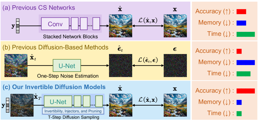
Figure 1: Proposed IDM compared to previous CS reconstruction paradigms. (a) Conventional NN-based CS methods (Chen et al., 2023a) develop and train new NN architectures from scratch. This constrains their capability to achieve high performance within a limited timeframe for rapid deployment. (b) Traditional diffusion model-based image reconstruction methods (Saharia et al., 2023) train a one-step noise estimation U-Net and employs it as an off-the-shelf NN module for iterative sampling. This estimator lacks an awareness of the entire recovery process from measurement to image, limiting its adaptability to CS. (c) Our invertible diffusion models (IDM) finetune a large-scale, pre-trained diffusion sampling process to directly predict original images from CS measurements end-to-end, significantly improving performance while reducing required sampling steps (Contribution 1). We also propose to make both the sampling process and noise estimation U-Net invertible, and add measurement injectors into our pruned noise estimation U-Net, leading to large performance boost, while greatly suppressing training GPU memory and running time (Contributions 2 and 3). Here, (a), (b), and (c) correspond to (12), (1), and (9) in Tab. 3, respectively. Please refer to Sec. 4.3 for details.

1 Introduction

Compressed sensing (CS) (Donoho, 2006) is a novel signal acquisition paradigm breaking through the limit of Nyquist-Shannon theorem (Shannon, 1949). It inspires a variety of applications including single-pixel imaging (SPI) (Duarte et al., 2008), magnetic resonance imaging (MRI) (Lustig et al., 2007), computational tomography (CT) (Chen et al., 2008; Szczykutowicz & Chen, 2010), and snapshot compressive imaging (SCI) (Yuan et al., 2021; Fu et al., 2021; Suo et al., 2023). In this paper, we focus on natural image CS reconstruction, which aims to predict the original image ${\mathbf{x}}\in{\mathbb{R}}^{N}$ from its linear measurements ${\mathbf{y}}\in{\mathbb{R}}^{M}$. The measurements are projected through a random sampling matrix ${\mathbf{A}}\in{\mathbb{R}}^{M\times N}$ with CS ratio $\gamma=M/N$ using ${\mathbf{y}}={\mathbf{A}}{\mathbf{x}}$. Typically, a low $\gamma$ value is preferred, with $M\ll N$, offering advantages such as reduced energy consumption and shorter acquisition times. However, this also introduces a challenge of reconstructing ${\mathbf{x}}$ from limited information of $\{{\mathbf{y}},{\mathbf{A}},\gamma\}$ due to the ill-posed nature of such an inverse problem.

In the field of natural image CS reconstruction, deep neural networks (NN) demonstrate greater effectiveness than traditional optimization-based methods (Zhang et al., 2014; Dong et al., 2014) in both accuracy and efficiency. Some early NN-based studies (Mousavi et al., 2015; Kulkarni et al., 2016) treat CS recovery as a de-aliasing problem, achieving fast and non-iterative reconstruction using a single forward pass of NN layers. Techniques such as algorithm unrolling (Monga et al., 2021), plug-and-play (PnP) (Zhang et al., 2022; Kamilov et al., 2023), and regularization by denoising (RED) (Romano et al., 2017) effectively decouple the encouragement of measurement consistency and deep image prior learning, striking a balance between performance and interpretability. Nonetheless, as Fig. 1 (a) illustrates, these methods typically require developing and training new NN architectures from scratch, a process that is not only time-consuming but also often leads to suboptimal performance.

Recently, diffusion models (Nichol & Dhariwal, 2021) are leveraged for image reconstruction in various works (Zhu et al., 2023; Saharia et al., 2023) to utilize pre-trained generative denoising priors. These approaches progressively sample an image estimate ${\hat{\mathbf{x}}}$ using iterative steps from the posterior distribution $p({\mathbf{x}}|{\mathbf{y}})$, yielding impressive measurement-conditioned synthesis (Zhu et al., 2023). Similar to PnP methods, current diffusion-based approaches focus on learning denoisers/noise estimators (Saharia et al., 2023), or employing pre-trained ones to solve image prior subproblems.

However, these methods often require extensive tuning of hyperparameters such as step size, regularization coefficient, and noise level. Furthermore, as Fig. 1 (b) illustrates, their NN backbones are primarily trained for one-step noise estimation, not optimized for the entire reconstruction process from CS measurements ${\mathbf{y}}$ to original image ${\mathbf{x}}$. In addition, previous diffusion-based inverse problem solvers (Zhang et al., 2019; Kawar et al., 2022; Song et al., 2023a; Chung et al., 2023a) can necessitate a considerable number of iterations or steps, varying from a minimum of 10 to as many as 1000, for generating satisfactory results. Methods utilizing latent diffusion models, such as stable diffusion (SD) (Rombach et al., 2022), typically require multi-stage training (Xia et al., 2023; Chen et al., 2023b; Wu et al., 2023; Wang et al., 2023a) or frequent data transitions between image and latent spaces via deep encoders and decoders during sampling (He et al., 2023; Fabian et al., 2023; Rout et al., 2023a), which compromises the efficiency of CS imaging systems.

To address these challenges, this paper proposes Invertible Diffusion Models (IDM) for image CS reconstruction, as shown in Fig. 1 (c). Moving beyond the constraints of one-step noise estimation learning in existing diffusion models, IDM establishes a novel end-to-end framework, which trains directly to align a large-scale, pre-trained diffusion sampling process with reconstruction mapping ${\mathbf{y}}\mapsto{\mathbf{x}}$. This alignment ensures that all the diffusion parameters and the weights of noise estimation U-Net are specifically optimized for image CS reconstruction, leading to significant performance improvements and eliminating the need for a large number of sampling steps. However, training such large diffusion models end-to-end demands high GPU memory, making it almost infeasible with commodity GPUs. To mitigate this, we leverage the memory efficiency of invertible NNs (Mangalam et al., 2022; Zhao et al., 2023) and propose a novel two-level invertible design. It introduces auxiliary connections into (1) the entire diffusion sampling framework comprising multiple steps and (2) the noise estimator within each step to transform both into invertible networks. This allows IDM to clear most intermediate features in the forward pass and recalculate them during back-propagation, hence significantly reducing GPU memory consumption.

Compared with previous end-to-end CS NNs that require training from scratch, IDM benefits from reusing pre-trained diffusion models, and adapts them to CS with minimal finetuning effort. In addition, we propose a series of lightweight NN modules dubbed as injectors that directly integrate measurement information into the deep features of noise estimation U-Net at different spatial scales to enhance reconstruction. Our method unlocks the power of pre-trained diffusion models to improve CS performance, paving a distinct way for the customized application of large diffusion models in image reconstruction. In summary, our contributions are:

❑ (1) We propose IDM, an efficient, end-to-end diffusion-based CS method. Unlike previous one-step diffusion noise estimation, IDM finetunes a large-scale sampling process for direct recovery from CS measurements end-to-end, improving performance by up to 4.34dB in PSNR with 98% step number reduction and $>$25 times inference acceleration.

❑ (2) We propose a novel two-level invertible design for both the sampling framework and noise estimation U-Net. This largely reduces the finetuning memory by up to 93.8%.

❑ (3) We propose a set of injectors that integrate CS measurements and sampling matrix into the noise estimation U-Net to facilitate CS reconstruction. These injectors effectively achieve $>$2dB PSNR improvements with only 0.02M additional parameters, compared to $>$100M in the U-Net.

❑ (4) We evaluate our IDM, as shown in Fig. 1 (c), across four typical tasks: natural image CS, inpainting, accelerated MRI, and sparse-view CT. It achieves a new state-of-the-art (SOTA) performance, surpassing existing CS NNs by up to 2.64dB in PSNR, while achieving up to 10.09dB PSNR gain and 14.54 times faster inference compared to the recent diffusion-based approach DDNM (Wang et al., 2023c, b).

2 Related Work

2.1 Deep End-to-End Learned Image CS Networks

Foundational deep NN-based CS researches (Mousavi et al., 2015; Iliadis et al., 2018) pioneer the use of fully connected layers to decode measurements into images. Convolutions (Kulkarni et al., 2016) and self-attention layers (Vaswani et al., 2017) give rise to more effective structures like residual blocks (He et al., 2016) and Transformers (Dosovitskiy et al., 2020; Ye et al., 2023). They capture both locality and long-range dependencies in images, popularizing expressive NN designs such as hierarchical and non-local architectures (Shi et al., 2019b; Cui et al., 2021). Recent works (Schlemper et al., 2017; Gilton et al., 2019; Chen & Davies, 2020) utilize the measurement information $\{{\mathbf{y}},{\mathbf{A}},\gamma\}$ to construct physics-informed CS NNs. Among these promising methodologies, deep unrolling (Aggarwal et al., 2018; Zhang et al., 2023), which reinterprets truncated optimization inferences as iterative NNs, establishing a new paradigm in this field. Compared to these studies, our work introduces powerful diffusion priors and avoids resource-intensive training from scratch. It enhances the efficiency of CS recovery learning.

2.2 Diffusion Model-Based Image Reconstruction

Denoising diffusion models (Sohl-Dickstein et al., 2015; Song & Ermon, 2019), particularly the denoising diffusion probabilistic models (DDPM) (Ho et al., 2020), emerges as effective generative priors for inverse imaging problems (Feng et al., 2023; Liu et al., 2023a, b; Delbracio & Milanfar, 2023; Chung et al., 2023b). The DDPM employs a $T$-step noising process ${\mathbf{x}}_{t}=\sqrt{\alpha_{t}}{\mathbf{x}}_{t-1}+\sqrt{1-\alpha_{t}}{\boldsymbol{\epsilon}}$, which can often be equivalently expressed as ${\mathbf{x}}_{t}=\sqrt{\bar{\alpha}_{t}}{\mathbf{x}}_{0}+\sqrt{1-\bar{\alpha}_{t}}{\boldsymbol{\epsilon}}$ utilizing the formulation of variance preserving stochastic differential equation (VP-SDE) (Song et al., 2021c). Here, ${\mathbf{x}}_{t}$ represents the sampled scaled and noisy image at step $t$, ${\boldsymbol{\epsilon}}\sim\mathcal{N}(\mathbf{0}_{N},\mathbf{I}_{N})$ is a random Gaussian noise, $\bar{\alpha}_{t}=\prod_{i=0}^{t}{\alpha_{i}}$ determines the scaling factors with $\alpha_{t}=1-\beta_{t}$ and noise schedule $\beta_{t}\in[0,1]$ $(\beta_{0}=0)$, while ${\mathbf{x}}_{0}$ is sampled from the clean image distribution $p({\mathbf{x}})$. Utilizing a pre-trained NN ${\boldsymbol{\epsilon}}_{\mathbf{\Theta}}$ that regresses $\min_{{\mathbf{\Theta}}}\lVert{\boldsymbol{\epsilon}}-{\boldsymbol{\epsilon}}_{\mathbf{\Theta}}(\sqrt{\bar{\alpha}_{t}}{\mathbf{x}}_{0}+\sqrt{1-\bar{\alpha}_{t}}{\boldsymbol{\epsilon}},t)\rVert_{2}^{2}$ with learnable parameter set ${\mathbf{\Theta}}$, given a starting point ${\hat{\mathbf{x}}}_{T}$, the denoising diffusion implicit model (DDIM) (Song et al., 2021b) can facilitate accelerated generation via a deterministic sampling strategy ${\hat{\mathbf{x}}}_{t-1}=\sqrt{\bar{\alpha}_{t-1}}{\hat{\mathbf{x}}}_{0|t}+\sqrt{1-\bar{\alpha}_{t-1}}{\hat{\boldsymbol{\epsilon}}}_{t}$, where ${\hat{\mathbf{x}}}_{0|t}={\left({\hat{\mathbf{x}}}_{t}-\sqrt{1-\bar{\alpha}_{t}}{\hat{\boldsymbol{\epsilon}}}_{t}\right)}/{\sqrt{\bar{\alpha}_{t}}}$ denotes the current denoised image, and ${\hat{\boldsymbol{\epsilon}}}_{t}={\boldsymbol{\epsilon}}_{\mathbf{\Theta}}({\hat{\mathbf{x}}}_{t},t)$ is the noise estimation.

Recent research (Saharia et al., 2022, 2023; Gao et al., 2023; Luo et al., 2023) regards image restoration as measurement-conditioned generation tasks. Zero-shot diffusion inverse problem solvers (Graikos et al., 2022) leverage the guidance of singular value decomposition (SVD) (Kawar et al., 2021, 2022), manifold constraints (Chung et al., 2022), posterior sampling (Jalal et al., 2021; Chung et al., 2023a), range-null space decomposition (RND) (Wang et al., 2023b, c), and pseudoinverse (Song et al., 2023b) for degradation operator-adaptive recovery. To the best of our knowledge, no existing diffusion models are specifically designed for natural image CS. Although many current methods can be applied for CS reconstruction, their noise estimation U-Nets are pre-trained for single-step noise estimation (see Fig. 1 (b)). Our work overcomes this limitation by aligning diffusion sampling with CS targets via end-to-end learning, improving performance while reducing the number of required steps.

2.3 Invertible Neural Networks for Vision Tasks

Invertible NNs, mathematically invertible functions, are a type of NNs that can reconstruct the input from output. They are initially used to generate images (Kingma & Dhariwal, 2018; Ho et al., 2019). Later literature finds that invertible NNs, unlike non-invertible ones caching all intermediate activations for gradient computation, allow freeing up most features that can be recomputed to reduce memory (Gomez et al., 2017). Following that, various invertible architectures are proposed, such as convolutional (Song et al., 2019), recurrent (MacKay et al., 2018), and graph (Li et al., 2021) NNs, as well as the Transformers (Mangalam et al., 2022; Zhao et al., 2023). Their application extends to image reconstruction (Liu et al., 2021; Huang & Dragotti, 2022), and image editing (Wallace et al., 2023b) with on-the-fly optimization in the latent space of autoencoders (Wallace et al., 2023a). The memory-efficiency property of invertible NNs is particularly appealing for training large diffusion models end-to-end. In this work, we propose a novel two-level invertible design for our end-to-end finetuning of large-scale pre-trained diffusion sampling process at minimal memory cost, making it practical with limited GPU resources.

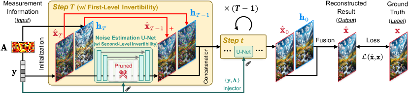
Figure 2: Illustration of our IDM framework. It receives an initialized estimation ${\hat{\mathbf{x}}}_{T}$ and learns $T$ diffusion sampling steps for recovery end-to-end. We perform “wiring” by introducing auxiliary connections (marked in red) for invertibility and reuse of pre-trained models.

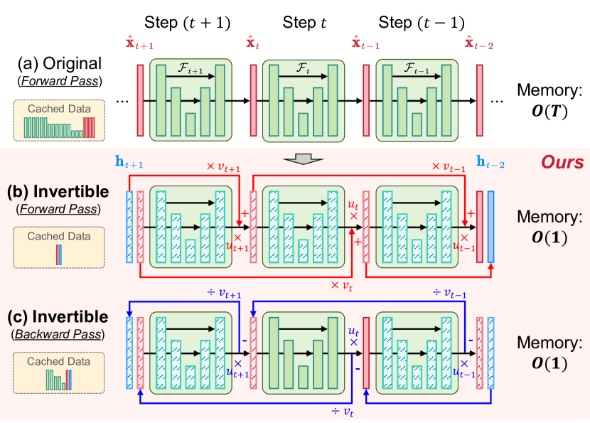
Figure 3: Illustration of our wiring technique, exampled with three diffusion sampling steps and a three-scale noise estimation U-Net. Here, the light-colored rectangles with diagonal dashed lines represent images/features that are cleared, while the dark-colored, empty rectangles indicate images/features that must be preserved. (a) Original non-invertible forward pass caches all inputs, features, and outputs, leading to their memory use linearly increasing with step number. (b) We add connections to construct invertible layers, reducing the memory use of images/features to be constant. (c) During back-propagation, the necessary intermediate inputs/features are recomputed and cleared sequentially to obtain gradients from the last to the first step. Our wired sampling framework is equivalent to the original (a) when $u_{t}=1$ and $v_{t}=0$.

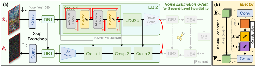
Figure 4: Illustration of our modified noise estimation U-Net ${\boldsymbol{\epsilon}}_{\mathbf{\Theta}}$ for CS tasks, based on SD v1.5 (Rombach et al., 2022). (a) We add injectors behind each residual and attention blocks, and wire them into groups in down-/up-sampling and middle blocks (marked as DB/UB/MB) for invertibility. Our method is orthogonal to and can be jointly utilized with pruning (Kim et al., 2023a) for enhanced efficiency. (b) Each injector learns to fuse measurement physics $\{{\mathbf{y}},{\mathbf{A}}\}$ into deep features using convolutions and residual connection.

3 Proposed Method

3.1 Preliminary

Denoising Diffusion Null Space Model (DDNM) and Its Limitations. DDNM (Wang et al., 2023c, b) is a training-free image reconstruction method that employs a pre-trained noise estimator ${\boldsymbol{\epsilon}}_{{\mathbf{\Theta}}}$ as generative prior and solves CS problem by iterating through the following three DDIM substeps:

$${\hat{\mathbf{x}}}_{0|t}=\left[{\hat{\mathbf{x}}}_{t}-\sqrt{1-\bar{\alpha}_{t}}{\boldsymbol{\epsilon}}_{\mathbf{\Theta}}({\hat{\mathbf{x}}}_{t},t)\right]/{\sqrt{\bar{\alpha}_{t}}},$$ (1)

$${\bar{\mathbf{x}}}_{0|t}={\mathbf{A}}^{\dagger}{\mathbf{y}}+(\mathbf{I}_{N}-{\mathbf{A}}^{\dagger}{\mathbf{A}}){\hat{\mathbf{x}}}_{0|t},$$ (2)

$${\hat{\mathbf{x}}}_{t-1}=\sqrt{\bar{\alpha}_{t-1}}{\bar{\mathbf{x}}}_{0|t}+\sqrt{1-\bar{\alpha}_{t-1}}{\boldsymbol{\epsilon}}_{\mathbf{\Theta}}({\hat{\mathbf{x}}}_{t},t).$$ (3)

Here, Eq. (1) predicts the denoised image, Eq. (2) applies the RND theory (Schwab et al., 2019; Chen & Davies, 2020) for measurement consistency ${\mathbf{A}}{\bar{\mathbf{x}}}_{0|t}={\mathbf{A}}{\mathbf{A}}^{\dagger}{\mathbf{y}}+{\mathbf{A}}(\mathbf{I}_{N}-{\mathbf{A}}^{\dagger}{\mathbf{A}}){\hat{\mathbf{x}}}_{0|t}\equiv{\mathbf{y}}$, and Eq. (3) executes a deterministic DDIM sampling, where ${\mathbf{A}}^{\dagger}\in{\mathbb{R}}^{N\times M}$ is the pseudoinverse of ${\mathbf{A}}$. However, the performance of DDNM is compromised due to a task shift from pre-training ${\boldsymbol{\epsilon}}_{{\mathbf{\Theta}}}$ on the noise estimation task in DDPM to its application in CS. The deep features within ${\boldsymbol{\epsilon}}_{{\mathbf{\Theta}}}$ are not necessarily optimized for mapping ${\mathbf{y}}$ to ${\mathbf{x}}$. Similar challenges exist in other diffusion-based methods, including zero-shot solvers (Chung et al., 2023a; Zhu et al., 2023) and conditional models (Saharia et al., 2022, 2023).

3.2 Learn Diffusion Sampling End-to-End for CS

Diffusion-based End-to-End CS Learning Framework. We hypothesize that directly fitting DDNM steps to recovery mapping ${\mathbf{y}}\mapsto{\mathbf{x}}$ end-to-end mitigates the task shift issues and enhances final performance. To this end, we construct a DDNM-based CS framework, which repurposes the DDNM sampling process as a $T$-layer NN ${\mathcal{F}}={\mathcal{F}}_{1}\circ{\mathcal{F}}_{2}\circ\cdots{\mathcal{F}}_{T}$, where each layer ${\hat{\mathbf{x}}}_{t-1}={\mathcal{F}}_{t}({\hat{\mathbf{x}}}_{t};{\mathbf{y}},{\mathbf{A}})$ represents a single sampling step encompassing Eqs. (1)-(3), with $\circ$ denoting the composition of sequential layers. Our framework finetunes both the diffusion parameters $\{\alpha_{t}\}$ and pre-trained weights in ${\boldsymbol{\epsilon}}_{{\mathbf{\Theta}}}$. It optimizes deep features to minimize the difference between estimation ${\hat{\mathbf{x}}}={\hat{\mathbf{x}}}_{0}={\mathcal{F}}({\hat{\mathbf{x}}}_{T};{\mathbf{y}},{\mathbf{A}})$ and ground truth ${\mathbf{x}}$ using an $\ell_{1}$ loss ${\mathcal{L}}({\hat{\mathbf{x}}},{\mathbf{x}})=\frac{1}{N}\lVert{\hat{\mathbf{x}}}-{\mathbf{x}}\rVert_{1}$ and standard back-propagation (Rumelhart et al., 1986). By doing so, our framework obtains a comprehensive adaptability to full recovery process and is not limited to learning noise estimation. This enhances its overall performance and introduces new gains orthogonal to the developments of solvers and text prompts (Chung et al., 2023c; Kim et al., 2023b).

Initialization Strategy of ${\hat{\mathbf{x}}}_{T}$ for CS Reconstruction. Contrary to typical diffusion models sampling from a random noise or those using NNs to estimate an initial result (Whang et al., 2022; Lin et al., 2023), we propose to use a simple yet effective initialization for ${\hat{\mathbf{x}}}_{T}$ by calculating an expectation ${\hat{\mathbf{x}}}_{T}={\mathbb{E}}_{{\boldsymbol{\epsilon}}}\left[\sqrt{\bar{\alpha}_{T}}{\hat{\mathbf{x}}}_{0}^{\prime}+\sqrt{1-\bar{\alpha}_{T}}{\boldsymbol{\epsilon}}\right]=\sqrt{\bar{\alpha}_{T}}{\mathbf{A}}^{\dagger}{\mathbf{y}}$ using back-projection ${\hat{\mathbf{x}}}_{0}^{\prime}=\left({\mathbf{A}}^{\dagger}{\mathbf{y}}\right)\in\arg\min_{{\mathbf{x}}}\lVert{\mathbf{A}}{\mathbf{x}}-{\mathbf{y}}\rVert_{2}^{2}$. This strategy enhances reconstruction quality at a low computational cost, surpassing the noise-initialized counterparts.

3.3 Two-Level Invertible Design for Memory Efficiency

Our end-to-end training improves performance but can challenge memory capacity of GPUs, especially with increased step number $T$ and a large noise estimator ${\boldsymbol{\epsilon}}_{\mathbf{\Theta}}$. This is due to the substantial footprint of intermediate features cached for back-propagation. For example, it is even impossible to directly train a diffusion sampling process with $T=3$ and SD v1.5 U-Net backbone end-to-end on 4 A100 GPUs with 80GB memory. To suppress memory consumption, we leverage the memory efficiency of invertible NNs and propose a novel two-level invertible design which makes both (1) the multi-step sampling framework and (2) the noise estimation NN invertible using a new “wiring” technique.

First-Level Invertibility for Multi-Step Sampling Framework. Inspired by Zhao et al. (2023), we propose to wire to enable invertibility by introducing new connections into the sampling steps, as Fig. 3 shows. Each connection transmits the input ${\hat{\mathbf{x}}}_{t}$ from one step ${\mathcal{F}}_{t}$ to the output ${\hat{\mathbf{x}}}_{t-2}$ of next step ${\mathcal{F}}_{t-1}$. We use two learnable weighting scalars $u_{t}$ and $v_{t}$ satisfying $u_{t}+v_{t}\equiv 1$ to scale the output of each step and the transmitted data respectively, and fuse them to obtain ${\hat{\mathbf{x}}}_{t-1}$. We introduce an auxiliary variable ${\mathbf{h}}_{t}$ and transform each layer into an invertible one, which can recover its input $\{{\hat{\mathbf{x}}}_{t},{\mathbf{h}}_{t}\}$ from a given output $\{{\hat{\mathbf{x}}}_{t-1},{\mathbf{h}}_{t-1}\}$ in a second pathway. Mathematically, the forward and inverse computations of each wired layer can now be formulated as:

Forward: $$\left\{\begin{aligned} &{\hat{\mathbf{x}}}_{t-1}=u_{t}{\mathcal{F}}_{t}({\hat{\mathbf{x}}}_{t};{\mathbf{y}},{\mathbf{A}})+v_{t}{\mathbf{h}}_{t},\\ &{\mathbf{h}}_{t-1}={\hat{\mathbf{x}}}_{t},\end{aligned}\right.$$ (4)

Inverse: $$\left\{\begin{aligned} &{\hat{\mathbf{x}}}_{t}={\mathbf{h}}_{t-1},\\ &{\mathbf{h}}_{t}={\left[{\hat{\mathbf{x}}}_{t-1}-u_{t}{\mathcal{F}}_{t}({\hat{\mathbf{x}}}_{t};{\mathbf{y}},{\mathbf{A}})\right]}/{v_{t}}.\end{aligned}\right.$$ (5)

To ensure the dimensions of our framework’s input and output remain consistent after wiring, we apply two learnable scalars $w_{T}$ and $w_{0}$ at the beginning and end, and compute the input and output as ${\mathbf{h}}_{T}=w_{T}{\hat{\mathbf{x}}}_{T}$ and ${\hat{\mathbf{x}}}={\hat{\mathbf{x}}}_{0}+w_{0}{\mathbf{h}}_{0}$, respectively. As illustrated in Figs. 3 (b) and (c), in the forward pass, we cache only the final output of wired layers, freeing up all intermediate features. After computing the loss function ${\mathcal{L}}$, we execute standard back-propagation layer-by-layer, from $\{{\hat{\mathbf{x}}}_{0},{\mathbf{h}}_{0}\}$ back to $\{{\hat{\mathbf{x}}}_{T},{\mathbf{h}}_{T}\}$. For layer $t$, we jointly recalculate its inputs, necessary features, and parameter gradients based on the outputs ${\hat{\mathbf{x}}}_{t-1}$ and ${\mathbf{h}}_{t-1}$, as well as their respective partial derivatives $\left(\partial{\mathcal{L}}/\partial{\hat{\mathbf{x}}}_{t-1}\right)$ and $\left(\partial{\mathcal{L}}/\partial{\mathbf{h}}_{t-1}\right)$ regarding the loss function ${\mathcal{L}}$. We implement an efficient memory management by clearing up all the cached intermediate features and outputs as we move through each layer from $t$ back to $(t+1)$.

Consequently, the memory of cached images and features in the framework is reduced from linear complexity ${\mathcal{O}}(T)$ to constant complexity ${\mathcal{O}}(1)$ when the sampling substeps and the architecture of noise estimation NN ${\boldsymbol{\epsilon}}_{\mathbf{\Theta}}$ are pre-determined. The developed wiring technique offers two advantages. Firstly, it can be applied to arbitrary diffusion models and solvers without the need to design new NNs. Secondly, we reuse the pre-trained weights of ${\boldsymbol{\epsilon}}_{\mathbf{\Theta}}$ for finetuning, with appropriate settings of $u_{t}$ and $v_{t}$. Our approach thereby leads to considerable savings in memory, time, and computation for improving reconstruction performance.

Second-Level Invertibility for Noise Estimator in Each Step. A U-Net architecture (Ronneberger et al., 2015) is generally utilized as noise estimator ${\boldsymbol{\epsilon}}_{\mathbf{\Theta}}$ in diffusion solvers. It includes multiple spatial scales with main and skip branches in both its down- and up-sampling blocks (Ma et al., 2023; Wimbauer et al., 2023). The blocks include complex, equidimensional transformations like residual and attention blocks (Rombach et al., 2022) that are memory-intensive. To further improve memory efficiency, we extend our wiring technique to U-Net blocks in each step. As depicted in Fig. 4 (a), we group and wire consecutive transformation blocks within each down-/up-sampling block to make them also invertible. During training, we clear all the input and intermediate activations from memory for these grouped blocks, while preserving only the features for the first/last convolutions and skip branches for back-propagation. This second-level invertible design further reduces memory and makes our IDM training feasible on standard consumer-grade GPUs.

Table 1: Comparison of average PSNR (dB, $\uparrow$) across various end-to-end learned methods on the luminance component of benchmark images. Throughout this paper, the best and second-best results of each case are highlighted in bold red and underlined blue, respectively.

Method	Test Set	Set11			CBSD68			Urban100			DIV2K
(Results of pre-2022 CS NNs are in Tab. 4)	CS Ratio $\gamma$	10%	30%	50%	10%	30%	50%	10%	30%	50%	10%	30%	50%
DGUNet+ (CVPR 2022) (Mou et al., 2022)		30.92	-	41.24	27.89	-	36.86	27.42	-	37.13	30.25	-	40.33
MR-CCSNet+ (CVPR 2022) (Fan et al., 2022)		-	-	39.27	-	-	35.45	-	-	34.40	-	-	38.16
FSOINet (ICASSP 2022) (Chen et al., 2022b)		30.44	37.00	41.08	28.12	33.15	37.18	26.87	33.29	37.25	30.01	36.03	40.38
CASNet (TIP 2022) (Chen & Zhang, 2022)		30.31	36.91	40.93	28.16	33.05	36.99	26.85	32.85	36.94	30.01	35.90	40.14
TransCS (TIP 2022) (Shen et al., 2022)		29.54	35.62	40.50	27.76	32.43	36.65	25.82	31.18	36.64	29.09	34.76	39.75
OCTUF+ (CVPR 2023) (Song et al., 2023a)		30.70	37.35	41.36	28.18	33.23	37.28	27.28	33.87	37.82	30.17	36.25	40.61
CSformer (TIP 2023) (Ye et al., 2023)		30.66	-	41.04	28.11	-	36.75	27.13	-	37.04	29.96	-	40.04
PRL-PGD+ (IJCV 2023) (Chen et al., 2023a)		31.70	37.89	41.78	28.50	33.41	37.37	28.77	34.73	38.57	30.75	36.64	40.97
IDM (Ours, $T=3$)		32.92	38.85	42.48	28.69	34.67	39.57	31.41	36.76	40.33	31.07	36.98	41.15

3.4 Inject Measurement Physics into Noise Estimator

The sufficient utilization of the physics information $\{{\mathbf{y}},{\mathbf{A}}\}$ is critical for CS reconstruction. If we only use it to initialize ${\hat{\mathbf{x}}}_{T}$ and RND-based step in Eq. (2), the reconstruction quality is limited in complex scenarios (as shown in Fig. 7 (5) vs. (9)), as it is difficult for the NN layers in ${\boldsymbol{\epsilon}}_{\mathbf{\Theta}}$ to learn the physics. Therefore, we need to inject the measurement physics directly into the layers. Simply appending measurement at the input layer of ${\boldsymbol{\epsilon}}_{\mathbf{\Theta}}$ in each step (Saharia et al., 2023) leads to unsatisfactory results, as the information in the random ${\mathbf{A}}$ and ${\mathbf{y}}$ can hardly be kept in deep NN features.

To address this, we propose a series of injectors, inspired by the success of physics-informed NNs (see Sec. 2.1). As illustrated in Fig. 4, each injector is positioned behind every grouped block within ${\boldsymbol{\epsilon}}_{\mathbf{\Theta}}$. For an intermediate deep feature ${\mathbf{F}}_{in}\in{\mathbb{R}}^{(H/r)\times(W/r)\times C}$ in U-Net, our injector fuses measurement physics information $\{{\mathbf{y}},{\mathbf{A}}\}$ and ${\mathbf{F}}_{in}$ as follows:

$${\mathbf{f}}=\text{Conv}_{1}\left(({\mathbf{F}}_{in})_{\uparrow r}\right)~{}\in{\mathbb{R}}^{H\times W\times 1}~{}(N=H\times W),$$ (6)

$${\mathbf{F}}_{out}={\mathbf{F}}_{in}+\left(\text{Conv}_{2}([{\mathbf{f}},{\mathbf{A}}^{\dagger}{\mathbf{A}}{\mathbf{f}},{\mathbf{A}}^{\dagger}{\mathbf{y}}])\right)_{\downarrow r}.$$ (7)

Here, $\text{Conv}_{1}$ and $\text{Conv}_{2}$ denote two $3\times 3$ convolutions that transition data between feature and image domains, $(\cdot)_{\uparrow/\downarrow r}$ is a Pixel-Shuffle/-Unshuffle layer of scaling ratio $r$, while $[{\mathbf{f}},{\mathbf{A}}^{\dagger}{\mathbf{A}}{\mathbf{f}},{\mathbf{A}}^{\dagger}{\mathbf{y}}]\in{\mathbb{R}}^{H\times W\times 3}$ is a channel-wise concatenation of intermediate image space data ${\mathbf{f}}$, its interaction with the CS sampling matrix ${\mathbf{A}}^{\dagger}{\mathbf{A}}{\mathbf{f}}$, and the back-projected measurement ${\mathbf{A}}^{\dagger}{\mathbf{y}}$. These lightweight injectors are jointly wired and learned within each block group in ${\boldsymbol{\epsilon}}_{\mathbf{\Theta}}$, establishing direct pathways that fuse measurement information and features, while effectively enhancing final recovery quality.

4 Experiment

4.1 Implementation Details of IDM

Architectural Customization. Moving beyond the original DDNM (Wang et al., 2023c, b) based on an unconditional image diffusion model (Dhariwal & Nichol, 2021) pre-trained on ImageNet dataset (Deng et al., 2009), our method reuses the noise estimation NN of SD v1.5 pre-trained on LAION dataset (Schuhmann et al., 2022) for its better performance after finetuning (see Tab. 3 (6) vs. (11)). We adapt this noise estimator to IDM by introducing Pixel-Unshuffle/-Shuffle layers of scaling ratio $s=2$ at the first/last convolutions to meet the four-channel data format of SD. As Fig. 4 (a) shows, we further simplify the U-Net by removing its time embeddings, cross-attention layers, and final three scales to balance efficiency and performance. Notably, this customized framework differs from other zero-shot, plug-and-play, or conditional models, as it allows rapid end-to-end finetuning of all reused weights for CS. This is advantageous for applications where there is a mismatch between the prior of modified, pre-trained diffusion model and the target task.

Table 2: Comparison of PSNR (dB, $\uparrow$)/SSIM ($\uparrow$), and time/storage complexity across diffusion-based methods on RGB test images.

Method	Test Set	Urban100 (100 RGB images of size $256\times 256$)			DIV2K (100 RGB images of size $256\times 256$)			Inference	Model Size
(FID/LPIPS results are in Tab. 7)	CS Ratio $\gamma$	10%	30%	50%	10%	30%	50%	Time (s, $\downarrow$)	(GB, $\downarrow$)
DDRM (NeurIPS 2022) (Kawar et al., 2022)		19.16/0.4348	28.91/0.8518	33.61/0.9365	20.91/0.4323	28.91/0.7852	33.68/0.9057	9.28	2.1
$\Pi$GDM (ICLR 2023) (Song et al., 2023c)		20.09/0.5089	26.70/0.7925	29.75/0.8724	22.46/0.5551	28.01/0.7714	30.79/0.8497	18.25	2.1
DPS (ICLR 2023) (Chung et al., 2023a)		17.12/0.3270	18.47/0.3891	19.21/0.4308	19.47/0.4222	20.78/0.4652	21.37/0.4884	19.02	2.1
DDNM (ICLR 2023) (Wang et al., 2023c)		20.76/0.4682	28.76/0.8284	32.86/0.9164	22.18/0.4383	28.50/0.7422	32.74/0.8726	9.16	2.1
GDP (CVPR 2023) (Fei et al., 2023)		20.74/0.5075	24.81/0.7086	26.12/0.7711	25.17/0.6334	27.75/0.7664	28.47/0.8029	21.35	2.1
PSLD (NeurIPS 2023) (Rout et al., 2023b)		19.43/0.4054	22.42/0.6399	22.78/0.6882	21.30/0.4427	23.87/0.6473	24.41/0.7124	233.10	4.3
SR3 (TPAMI 2023) (Saharia et al., 2023)		18.90/0.5023	21.37/0.6428	23.12/0.7233	20.10/0.4794	22.07/0.5689	23.63/0.6518	35.62	0.4
IDM (Ours, $T=3$)		30.85/0.8970	35.78/0.9570	39.16/0.9771	31.22/0.8581	36.83/0.9482	40.81/0.9755	0.63	0.4

All Learnable Parameters in IDM are jointly finetuned end-to-end, including the shared, wired U-Net ${\boldsymbol{\epsilon}}_{\mathbf{\Theta}}$ and its internal weighting factors (i.e., $v_{i}$s with $u_{i}\equiv 1-v_{i}$) across the $T$ sampling steps, the non-shared and step-specific diffusion parameters $\{\alpha_{t}\}$, weighting scalars $\{v_{t}\}$ with $u_{t}\equiv 1-v_{t}$ for our invertible diffusion sampling pipeline, the scaling factors $w_{T}$ and $w_{0}$, as well as the parameters of our designed $(20T)$ injectors. The values of scalars $\alpha_{t}$, $v_{t}$, $v_{i}$, $w_{T}$, and $w_{0}$ are initialized to 0.5, 0.5, 0.5, 1.0, and 0.0, respectively.

Ground Truth	CSNet+	OPINE-Net+	TransCS	PRL-PGD+	IDM (Ours)
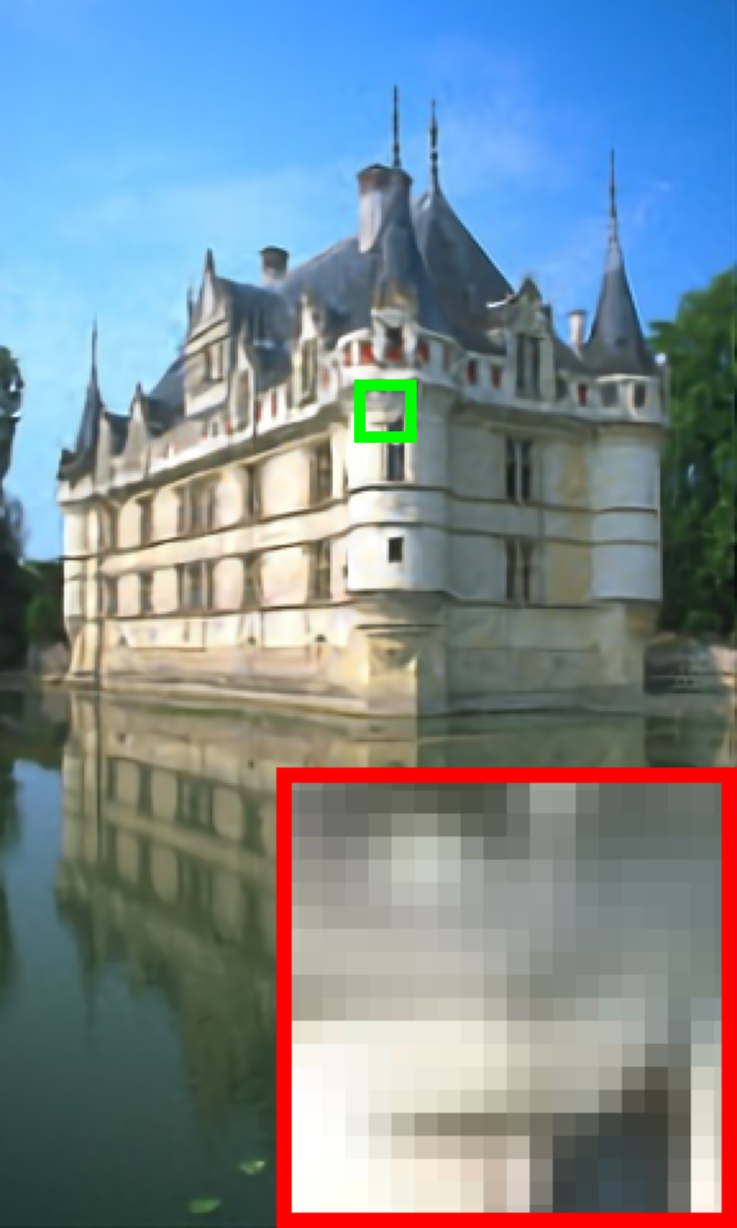
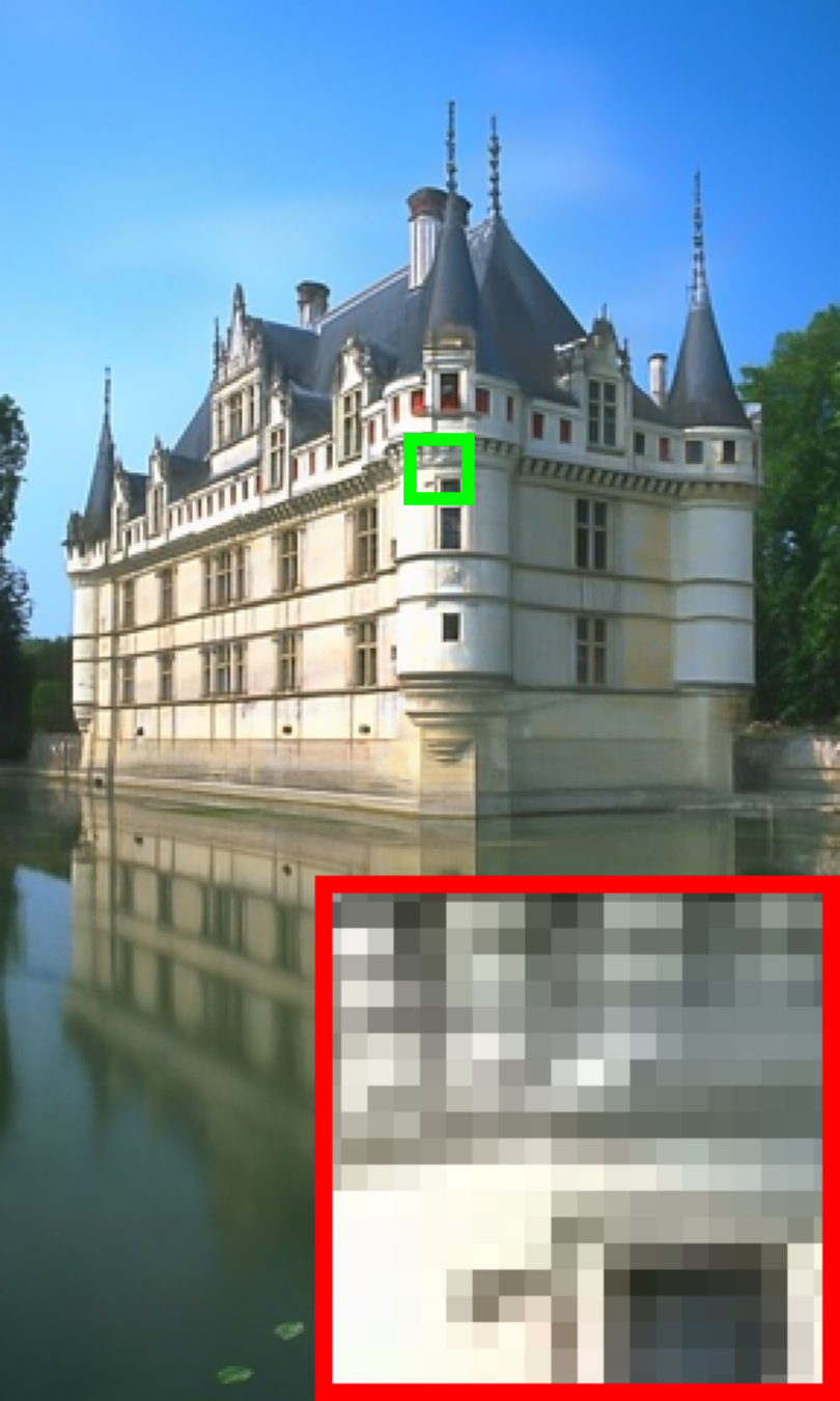
PSNR/SSIM	26.09/0.8369	26.56/0.8544	26.82/0.8594	28.11/0.8855	31.02/0.8859

Figure 5: Comparison of CS recovery results from end-to-end learned methods on “test_03” image from CBSD68 at $\gamma=10\%$.

Ground Truth	${\mathbf{A}}^{\dagger}{\mathbf{y}}$	DDRM	$\Pi$GDM	DPS
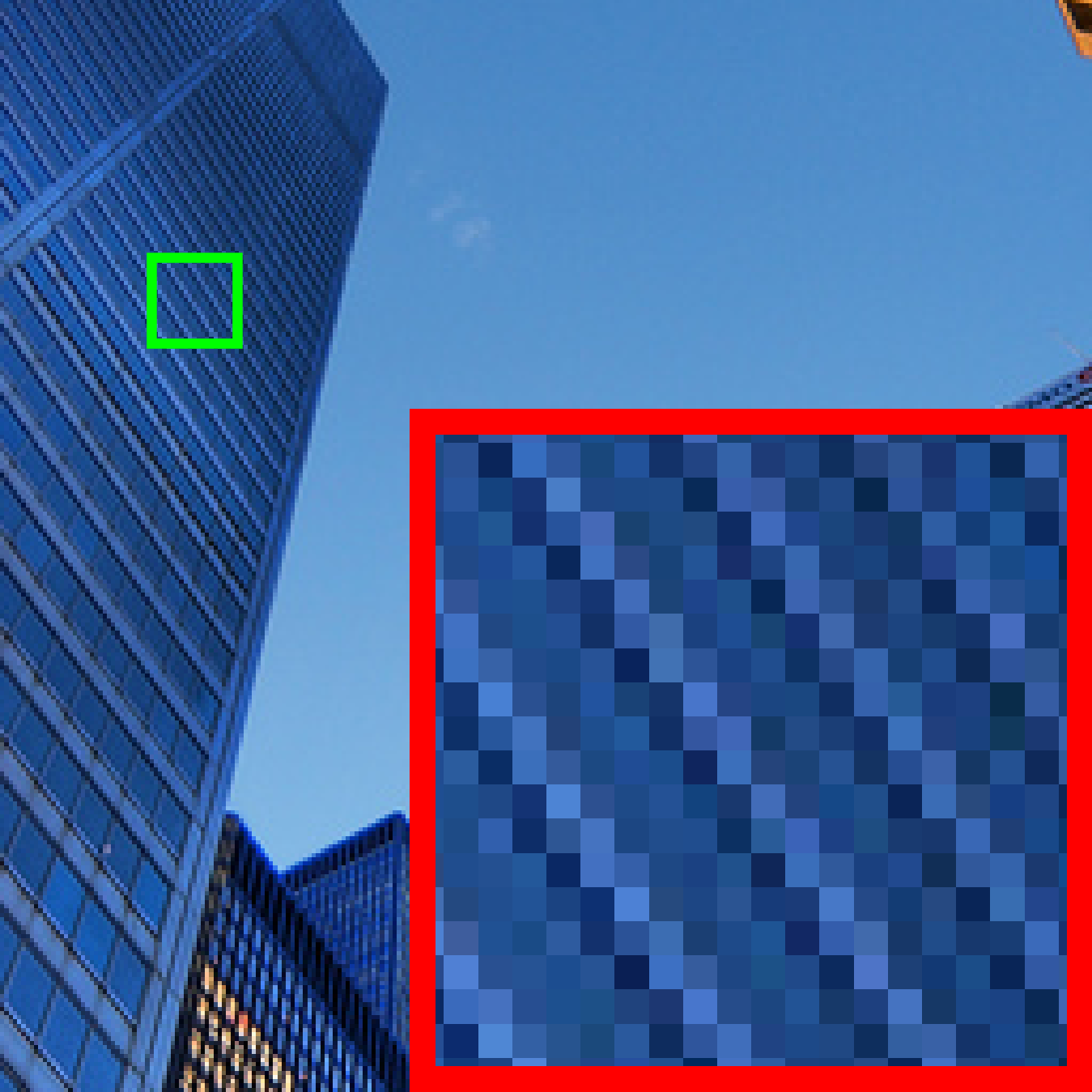
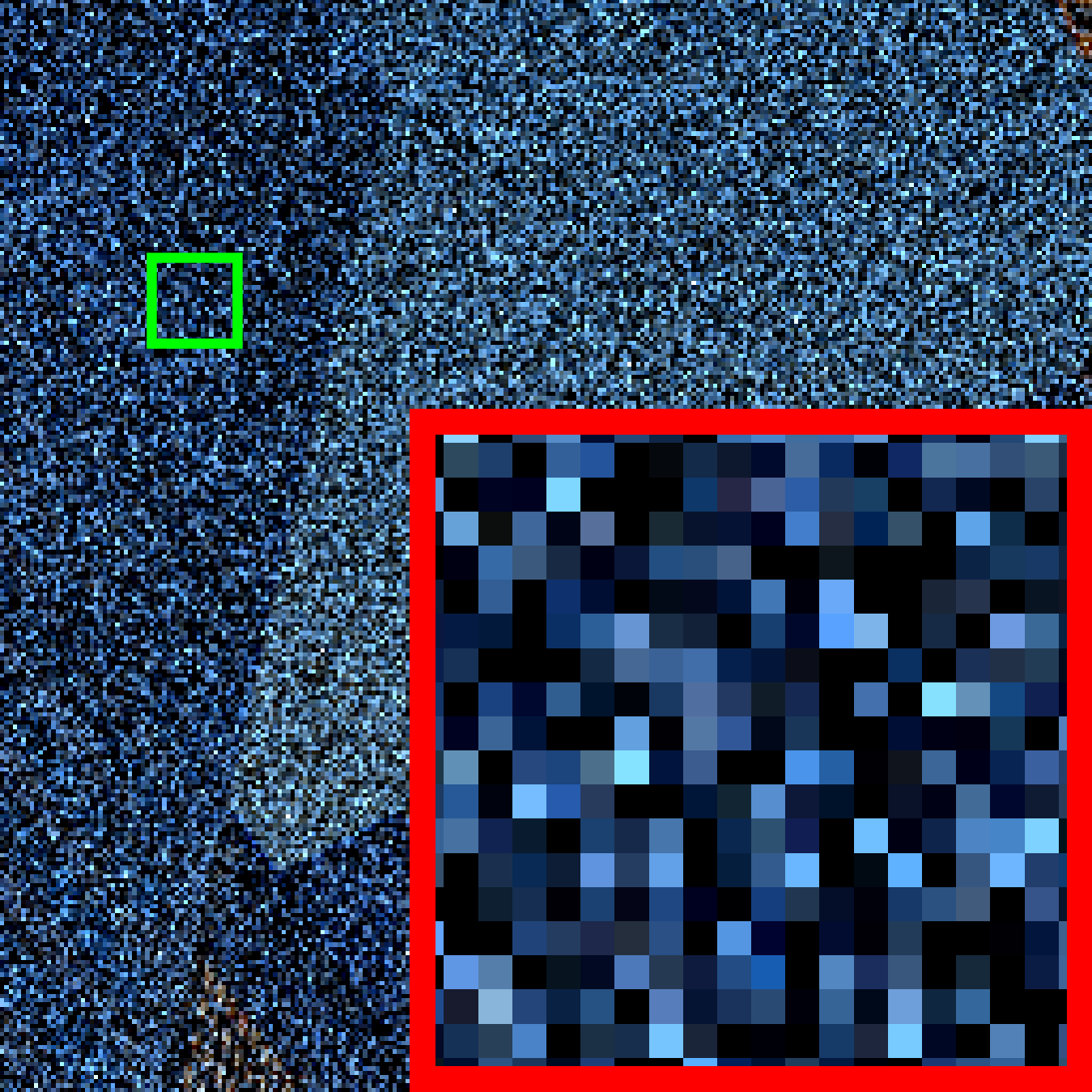
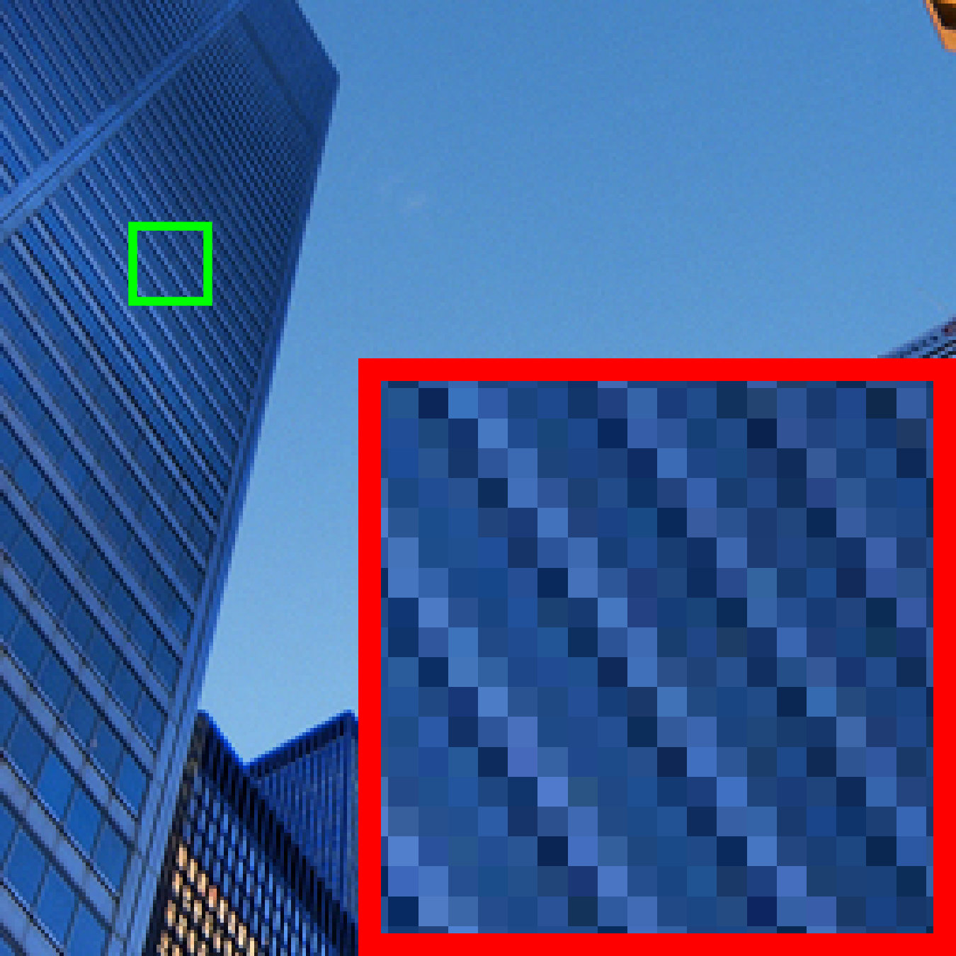
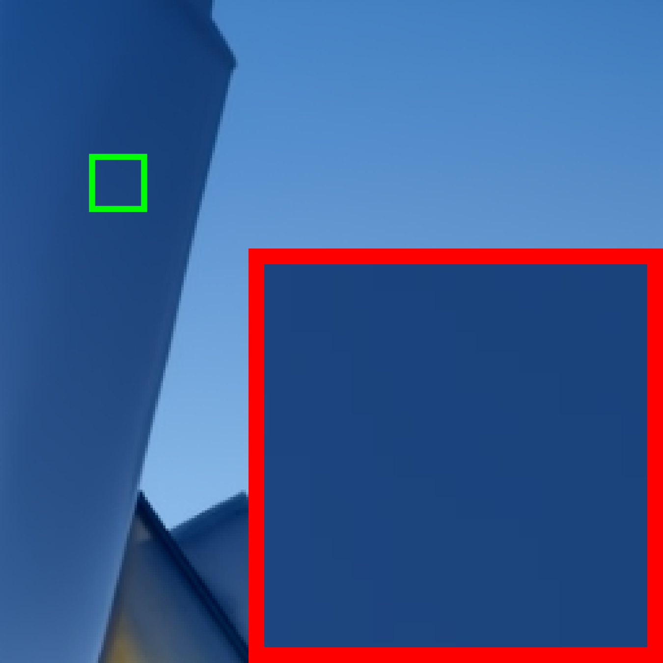
PSNR/SSIM	8.79/0.0600	36.20/0.9330	27.76/0.8317	22.27/0.7109

DDNM	GDP	PSLD	SR3	IDM (Ours)
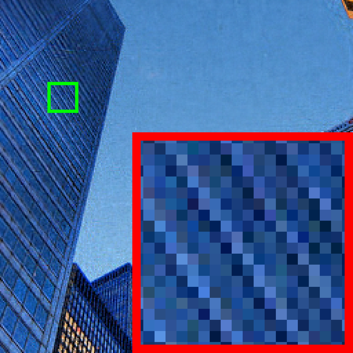
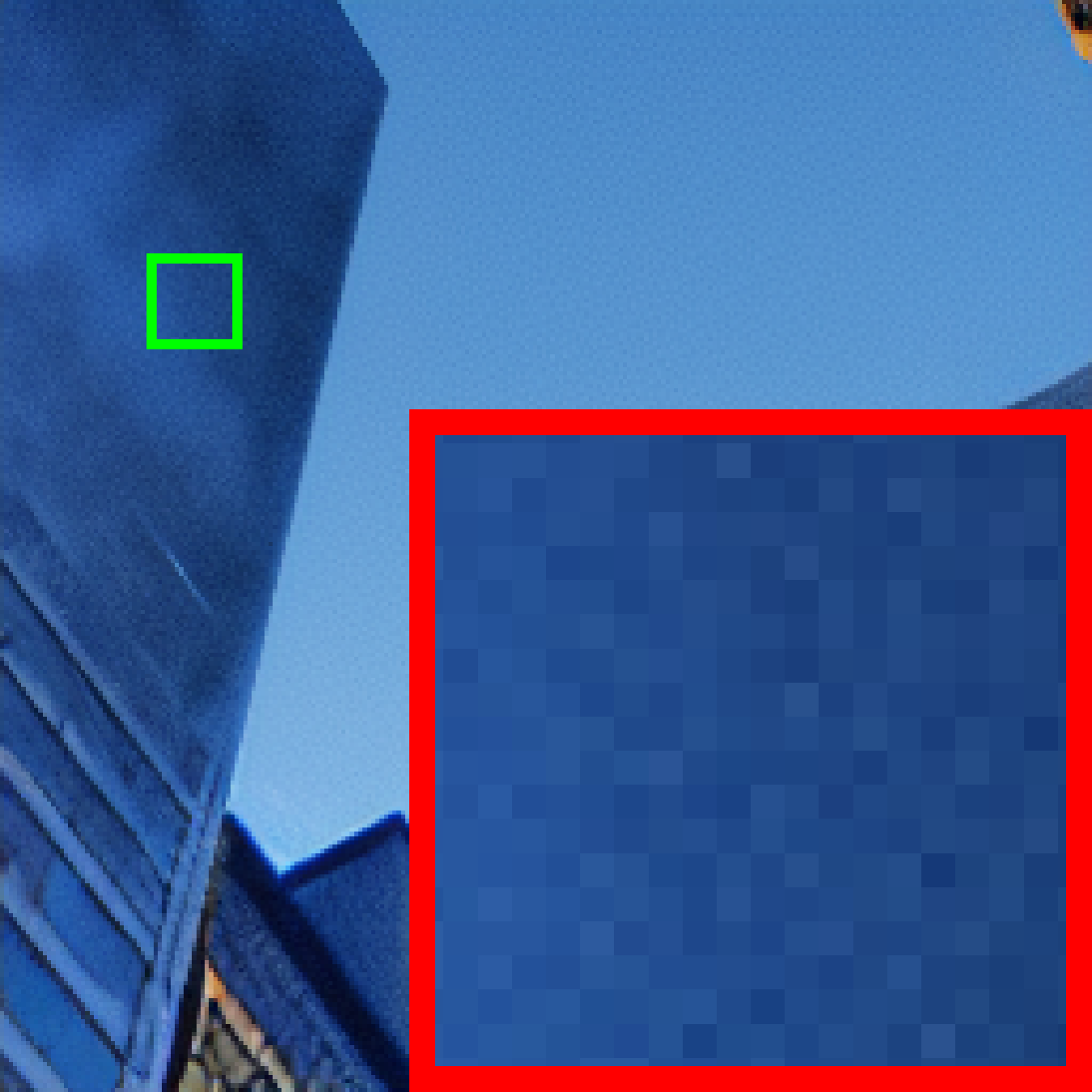
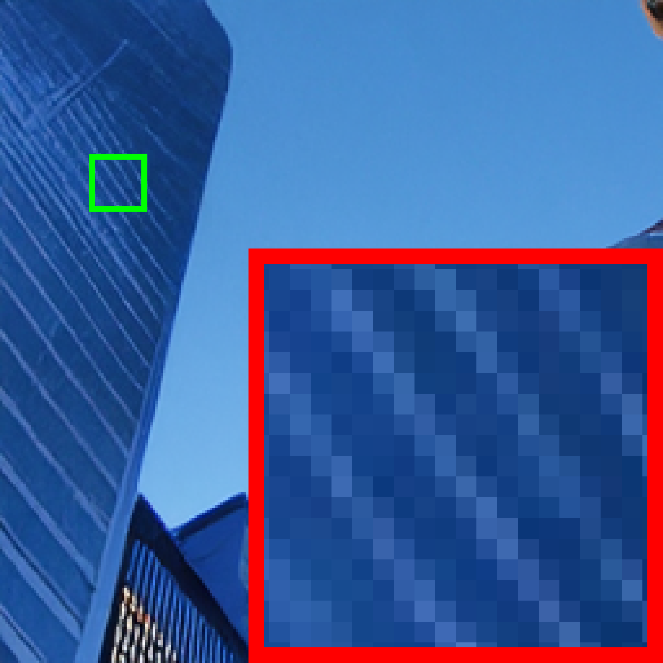
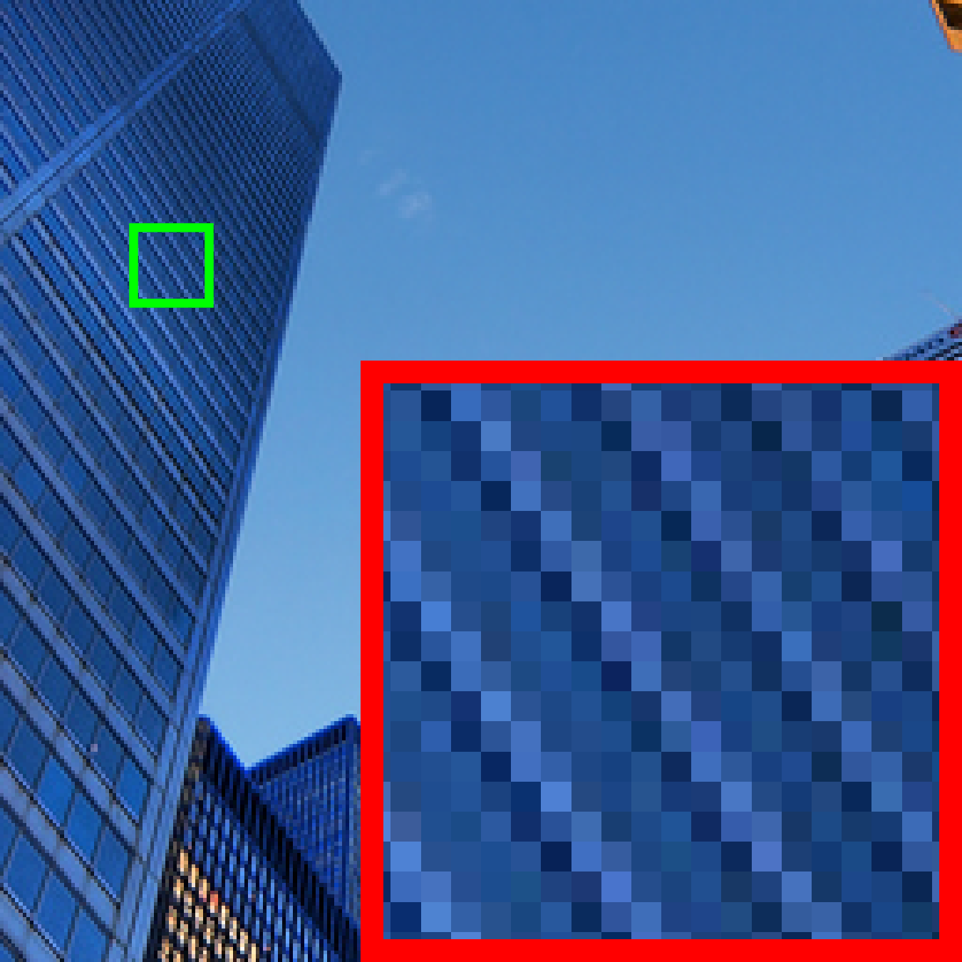
37.41/0.9319	30.30/0.8325	24.94/0.7217	25.27/0.8171	45.26/0.9882

Figure 6: Comparison of CS recovery results from diffusion-based methods on “img_012” image from Urban100 at $\gamma=50\%$.

4.2 Comparison with Existing Methods

Setup. IDM is compared against twenty end-to-end learned and eight diffusion-based approaches for natural image CS tasks. Training data pairs $\{({\mathbf{y}},{\mathbf{x}})\}$ are generated from the randomly cropped $256\times 256$ patches of Waterloo exploration database (WED) (Ma et al., 2016; Zhang et al., 2022; Li et al., 2022; Chen et al., 2023a) using structurally random, orthonormalized i.i.d. Gaussian matrices ${\mathbf{A}}$ of a fixed block size $32\times 32$ (Do et al., 2012; Adler et al., 2017; Chen et al., 2021). Finetuning IDM with $T=3$ and a batch size of 32 for 50000 iterations on 4 A100 (80GB) GPUs and PyTorch (Paszke et al., 2019) takes three days, with a starting learning rate of 0.0001, halved every 10000 iterations. Four benchmarks: Set11 (Kulkarni et al., 2016), CBSD68 (Martin et al., 2001), $256\times 256$ center-cropped Urban100 (Huang et al., 2015), and DIV2K (Agustsson & Timofte, 2017) are employed. For RGB images, we sample each R/G/B channel separately, and multiply input/output channel numbers of first/last convolutions in U-Net and injectors by 3. Peak signal-to-noise ratio (PSNR) and structural similarity index measure (SSIM) (Wang et al., 2004) are employed as metrics. Results of existing methods are sourced from original publications, or obtained via careful hyperparameter tuning and re-training. In cases where replicable algorithms are not available, we indicate this in our tables using a “-” symbol. Especially, for SR3, we adopt ${\mathbf{A}}^{\dagger}{\mathbf{y}}$ as its conditional input.

Ground Truth	${\mathbf{A}}^{\dagger}{\mathbf{y}}$	(1) DDNM	(5) w/o Inj.	(9) Ours
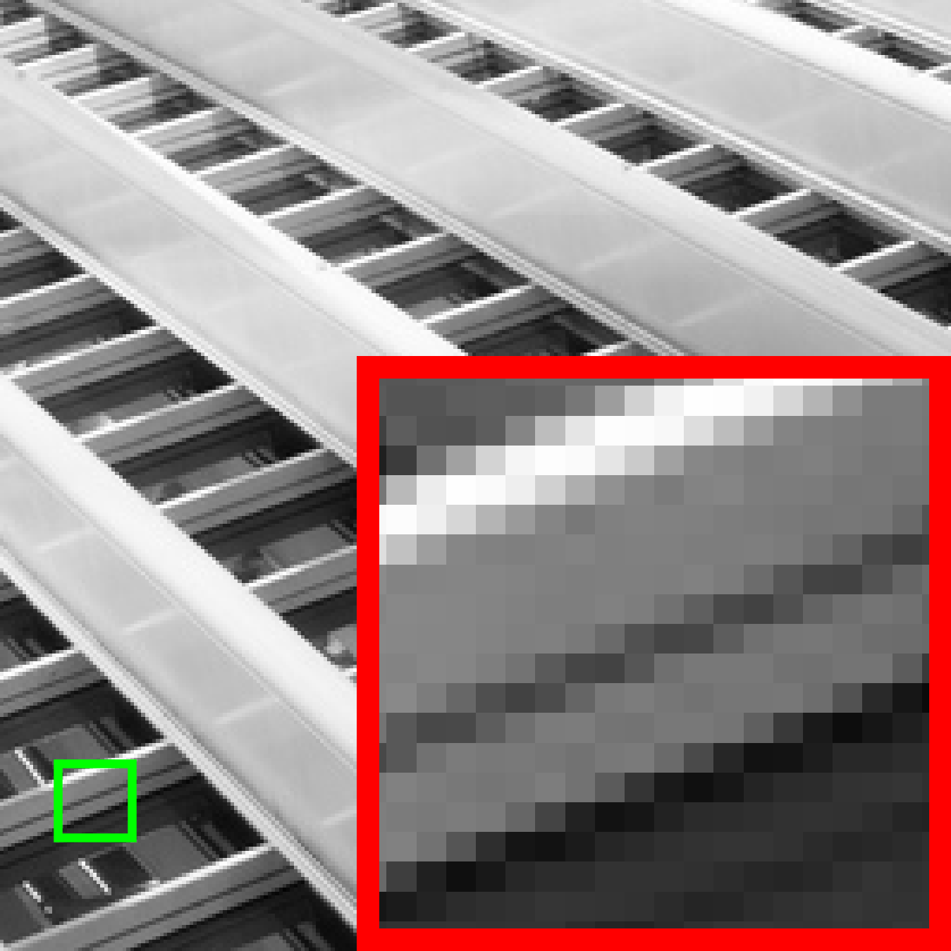
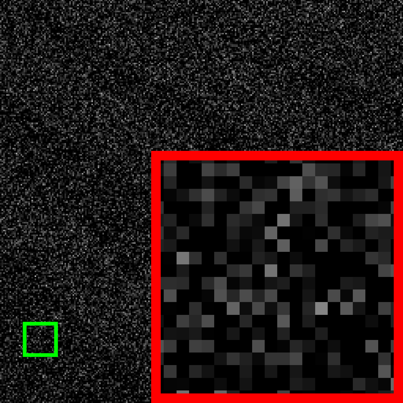
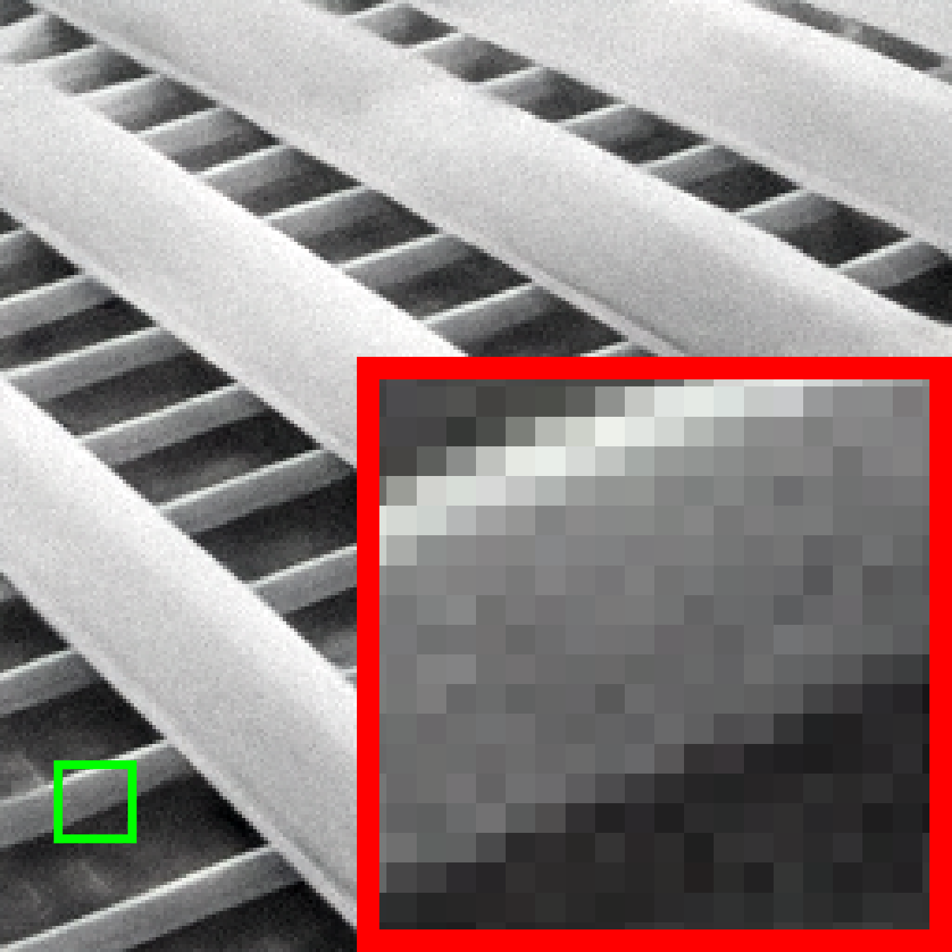
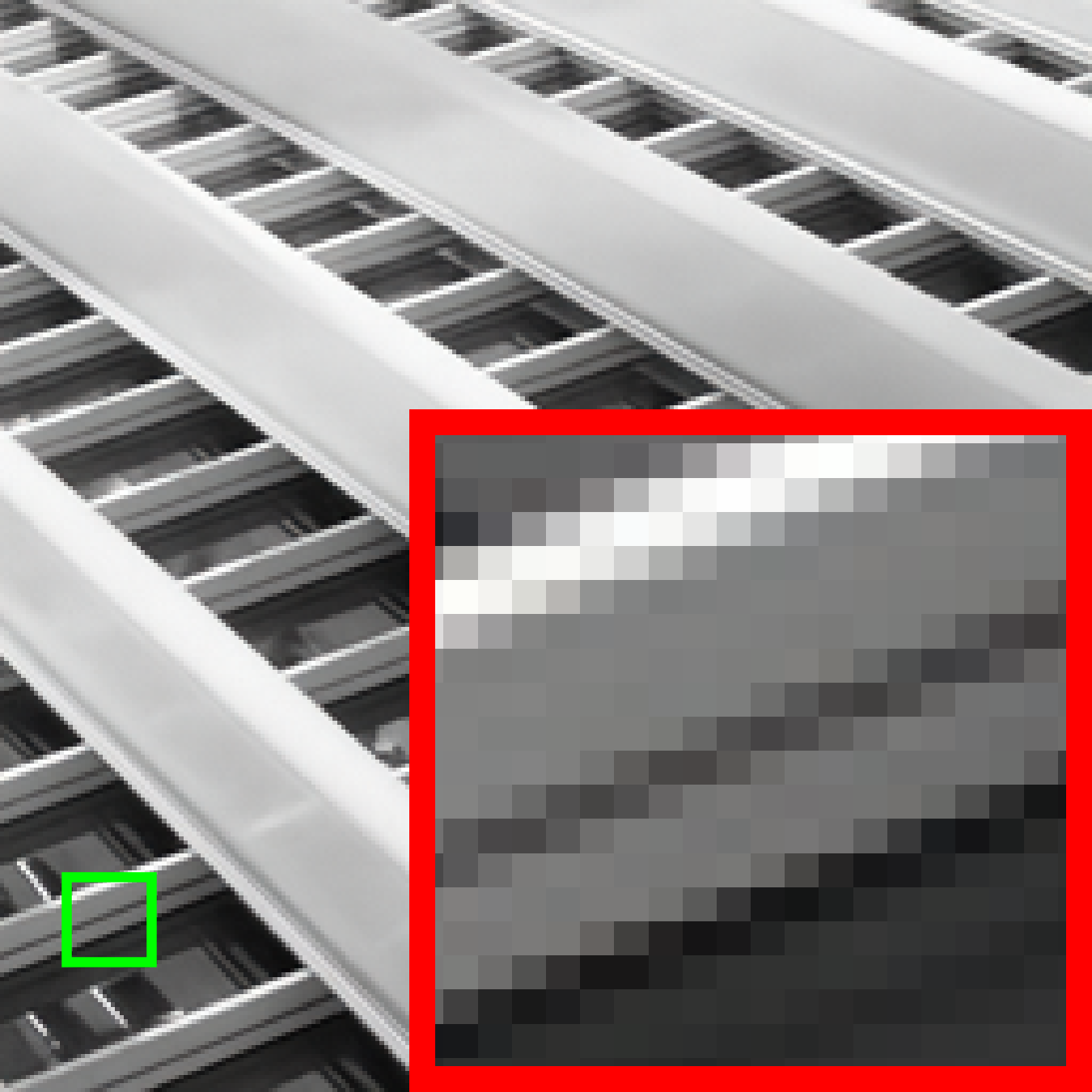
PSNR/SSIM	4.87/0.0293	26.21/0.7802	24.20/0.7446	34.18/0.9550
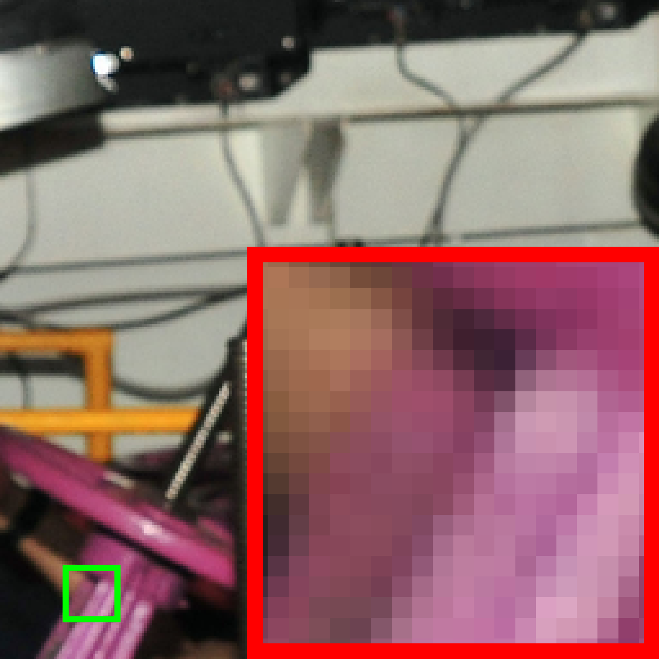
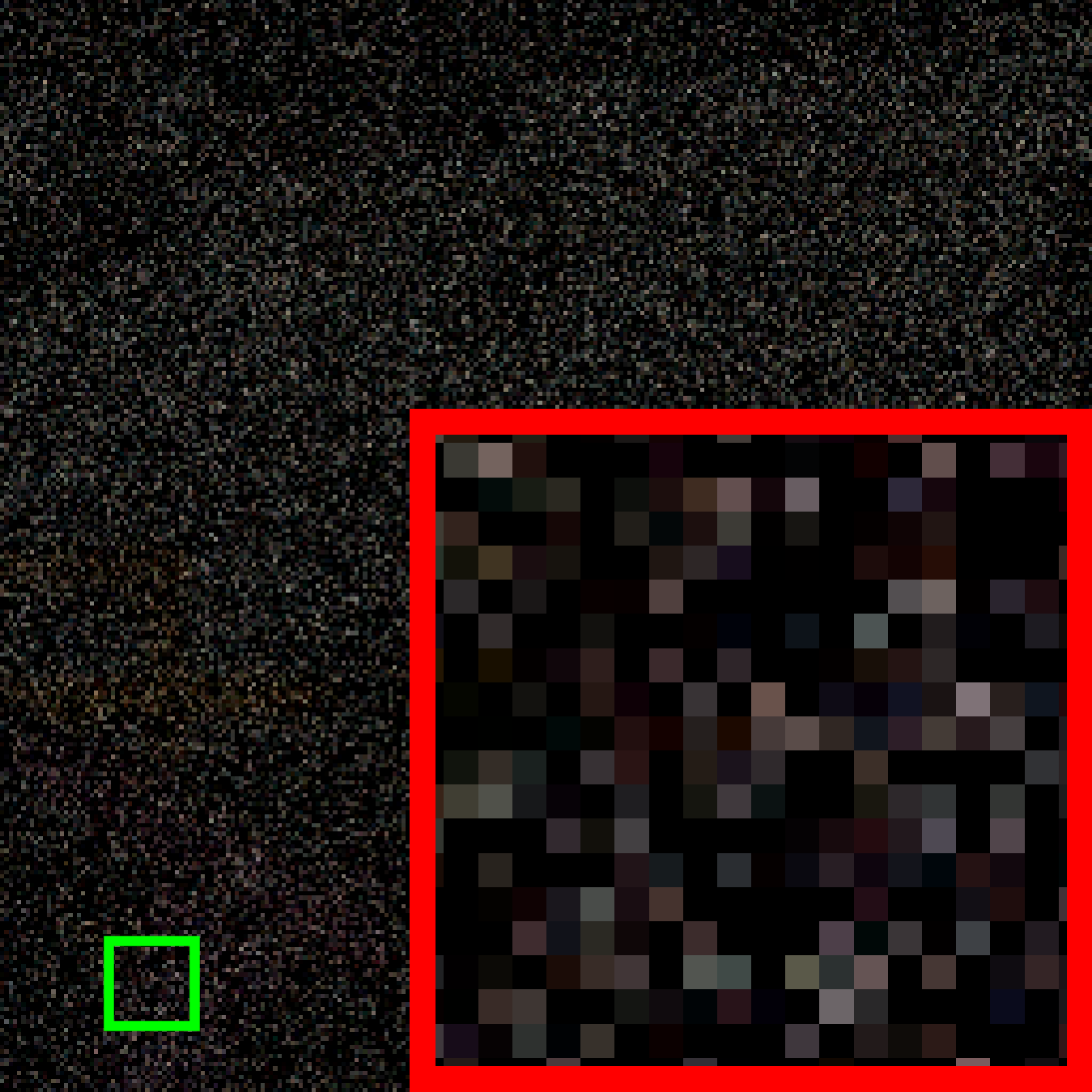
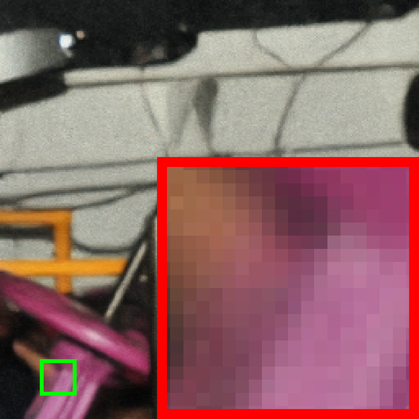
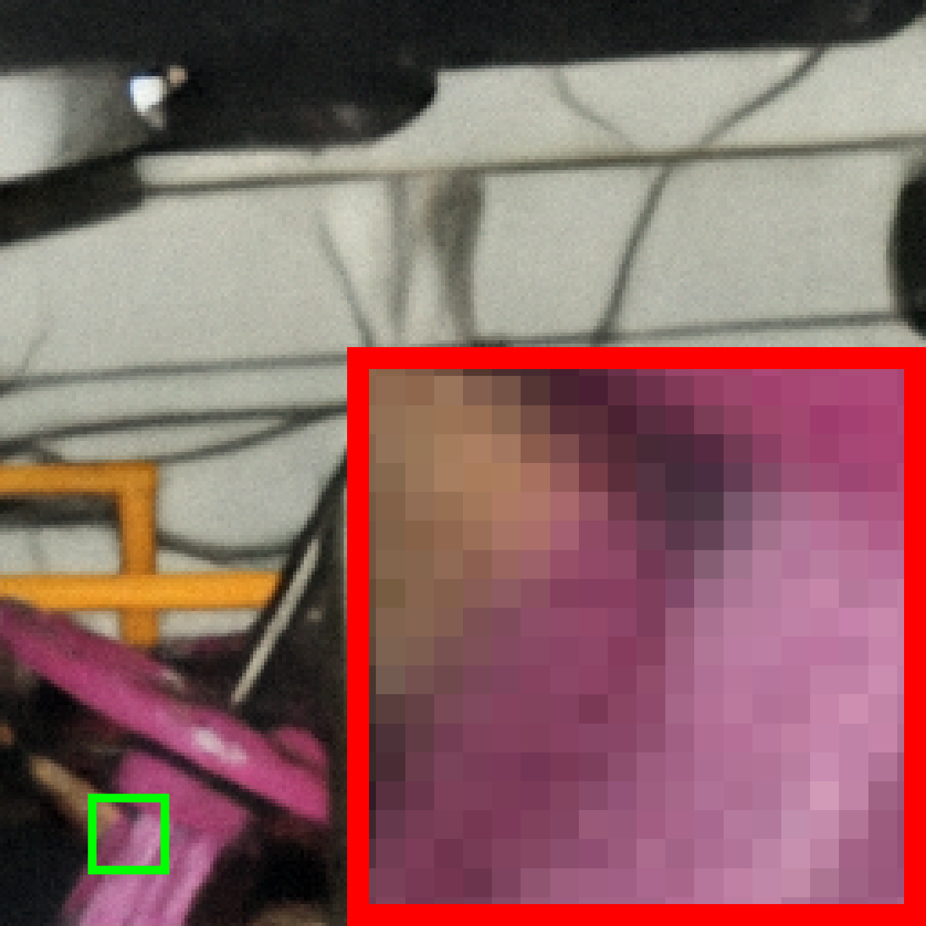
PSNR/SSIM	7.02/0.0446	28.42/0.8201	27.72/0.8315	37.20/0.9693

Figure 7: Comparison of CS recovery results from the method variants of (1), (5), and (9) in Tab. 3 on the “img_042” and “0888” images from Urban100 (top) and DIV2K (bottom) at $\gamma=10\%$.

Results. Tab. 1 exhibits that our IDM outperforms other end-to-end learned CS NNs, notably exceeding PRL-PGD⁺ by an average PSNR margin of 0.96/1.22/2.14/0.48dB on the four benchmark datasets. As illustrated in Fig. 5, IDM yields accurate, high-faithfulness details, especially on the building edges and windows. In contrast, eight other competing CS NNs can result in oversmoothed and blurry building textures. IDM minimizes artifacts and leads in PSNR, outperforming the second-best image CS approach PRL-PGD⁺ by 2.91dB.

Tab. 2 demonstrates the substantial advantage of our method in PSNR/SSIM, outperforming the second-best contenders by an average margin of 7.27dB/0.1652. Such an enhanced performance can be attributed to the ability of our method to address the shortcomings of generative priors in maintaining data fidelity and the insufficient adaptation to CS tasks of their noise estimators. As depicted in Fig. 6, while DDRM, DDNM, and GDP can synthesize high-quality patterns in the areas of building windows, they also generate noise-like artifacts in the regions of sky and windows. Although $\Pi$GDM, DPS, PSLR, and SR3 reconstruct the basic shapes and structures of the original image, they struggle to recover detailed features of the building facade, which can be observed in the zoomed-in area. Notably, SR3 requires 240 hours and 75GB memory per GPU for training. Our IDM stands out by necessitating only 76 hours and 15GB memory per GPU, delivering high-quality, artifact-free images using merely 3 NFEs for the noise estimator—a stark contrast to the $\geq$100 NFEs required by competing methods. This results in an inference speed-up of approximately 15-370 times. These above observations validate the effectiveness of our end-to-end finetuning framework for diffusion sampling learning, and wiring technique for two-level invertibility and reuse.

Table 3: Ablation study on our contributions and developed techniques for performance/efficiency enhancement. Arch.: Architecture choice of noise estimator. E2E: End-to-end training. Inv.: Invertibility. Reu.: Reuse of pre-trained NN weights. Inj.: Injectors. Pru.: Pruning. PSNR: Average PSNR (dB) of RGB image CS on Urban100/DIV2K at $\gamma=10\%$. Mem.: GPU memory usage (GB). Tra. $t$: Training time (hours) for convergence. NFEs: Neural function evaluations. Inf. $t$: Inference time per image (s). Size: Storage size (GB). X^∗: Modified version of method “X”. UIDM: Unconditional image diffusion model (Dhariwal & Nichol, 2021). N/A: Not applicable.

Method Variant

Arch. of ${\boldsymbol{\epsilon}}_{\mathbf{\Theta}}$

E2E

Inv.

Reu.

Inj.

Pru.

Initialization

PSNR ($\uparrow$)

Mem. ($\downarrow$)

Tra. $t$ ($\downarrow$)

NFEs ($\downarrow$)

Inf. $t$ ($\downarrow$)

Size ($\downarrow$)

(1)

DDNM∗

✘

✘

✘

✘

✘

${\hat{\mathbf{x}}}_{T}\sim\mathcal{N}(\mathbf{0}_{N},\mathbf{I}_{N})$

22.86/25.13

22.3

417.3

100

42.30

3.4

(2)

DDNM∗

✘

✘

✔

✘

✘

${\hat{\mathbf{x}}}_{T}\sim\mathcal{N}(\mathbf{0}_{N},\mathbf{I}_{N})$

24.28/26.25

22.3

40.6

100

42.37

3.4

(3)

IDM∗

✔

✘

✘

✘

✘

${\hat{\mathbf{x}}}_{T}=\sqrt{\bar{\alpha}_{T}}{\mathbf{A}}^{\dagger}{\mathbf{y}}$

26.17/28.09

34.6

411.1

2

1.72

3.4

(4)

IDM∗

✔

✔

✘

✘

✘

${\hat{\mathbf{x}}}_{T}=\sqrt{\bar{\alpha}_{T}}{\mathbf{A}}^{\dagger}{\mathbf{y}}$

26.21/28.14

13.4

820.7

2

1.69

3.4

(5)

IDM∗

✔

✘

✔

✘

✘

${\hat{\mathbf{x}}}_{T}=\sqrt{\bar{\alpha}_{T}}{\mathbf{A}}^{\dagger}{\mathbf{y}}$

26.57/28.33

34.6

12.4

2

1.69

3.4

(6)

IDM∗

✔

✔

✔

✘

✘

${\hat{\mathbf{x}}}_{T}=\sqrt{\bar{\alpha}_{T}}{\mathbf{A}}^{\dagger}{\mathbf{y}}$

26.52/28.31

13.4

24.5

2

1.68

3.4

(7)

IDM∗

✔

✔

✔

✔

✘

${\hat{\mathbf{x}}}_{T}=\sqrt{\bar{\alpha}_{T}}{\mathbf{A}}^{\dagger}{\mathbf{y}}$

29.53/30.41

13.4

26.4

2

1.77

3.4

(8)

IDM∗

✔

✔

✔

✔

✔

${\hat{\mathbf{x}}}_{T}\sim\mathcal{N}(\mathbf{0}_{N},\mathbf{I}_{N})$

27.21/29.12

5.0

8.3

2

0.38

0.4

(9)

IDM (Ours)

SD v1.5

✔

✔

✔

✔

✔

${\hat{\mathbf{x}}}_{T}=\sqrt{\bar{\alpha}_{T}}{\mathbf{A}}^{\dagger}{\mathbf{y}}$

29.44/30.37

4.9

8.0

2

0.38

0.4

(10)

DDNM

✘

✘

✔

✘

✘

${\hat{\mathbf{x}}}_{T}\sim\mathcal{N}(\mathbf{0}_{N},\mathbf{I}_{N})$

20.76/22.18

N/A

N/A

100

9.16

2.1

(11)

IDM∗

UIDM

✔

✔

✔

✘

✘

${\hat{\mathbf{x}}}_{T}=\sqrt{\bar{\alpha}_{T}}{\mathbf{A}}^{\dagger}{\mathbf{y}}$

24.45/26.52

18.4

4.2

2

0.33

2.1

(12)

PRL-PGD+

N/A

✔

✘

✘

✘

✘

${\hat{\mathbf{X}}}^{(0)}=\text{Conv}({\mathbf{A}}^{\dagger}{\mathbf{y}})$

26.74/28.32

8.6

652.4

N/A

0.95

0.8

4.3 Ablation Study and Analysis

Setup. We evaluate scaled-down IDM variants trained on an A100 GPU with $T=2$, a batch size of 4, and a patch size of 128 in this section. Results are in Tab. 3 and Figs. 7-9. Two SOTAs: DDNM (Wang et al., 2023c) and end-to-end PRL-PGD⁺ (Chen et al., 2023a) re-trained for RGB image CS, are included as references in (10) and (12). We also train two measurement-conditioned SD-based DDNM variants in (1) and (2) (Saharia et al., 2023; Rombach et al., 2022).

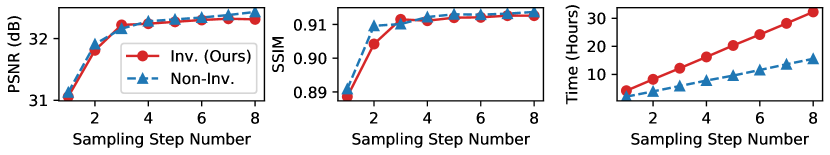
Figure 8: Comparison of IDM variants with $1\leq T\leq 8$. We evaluate PSNR ($\uparrow$)/SSIM ($\uparrow$) for the luminance component image CS on Set11 at $\gamma=10\%$ (left/middle) and training time cost ($\downarrow$) (right). Parameter number is calculated as $(115.254+0.006T)$M.

Figure 9: Comparison of IDM variants with $1\leq T\leq 12$. We evaluate memory use ($\downarrow$) on A100 (80GB) GPU (left), and maximum batch size ($\uparrow$) for training on 1080Ti (11GB) GPU (right). Notably, our IDM reduces memory by 93.8% ($\approx$15/16) at $T=12$.

Effect of End-to-End DDNM Sampling Learning. Comparisons (1) vs. (3), (2) vs. (5), and (10) vs. (11) in Tab. 3 exhibit that our end-to-end DDNM sampling learning provides substantial PSNR improvements of 2.06-4.34dB. It also decreases the required step number by 98% and boosts inference speed by 27.55-29.50 times. Notably, the method variant (11) needs only 4.2 hours of finetuning, validating the efficiency and rapid deployment capability of our IDM.

Effect of Two-Level Invertible Design, and Reuse. Comparisons of (3) vs. (4) and (5) vs. (6) in Tab. 3 exhibit that our wired models achieve a 61.3% reduction in memory usage while effectively maintaining recovery performance. Fig. 9 demonstrates that our two-level wiring scheme consistently keeps memory usage within only 3-4GB and scales maximum batch size by a factor of 3, improving the overall training efficiency on modern GPUs (Mangalam et al., 2022). As Fig. 8 (right) shows, invertibility (Inv.) can double training time, due to recomputation during back-propagation. Fortunately, we reuse the pre-trained models. Comparisons of (1) vs. (2), (3) vs. (5), and (4) vs. (6) exhibit that weight reuse brings 0.17-1.42dB PSNR improvements and 90.3-97.0% time reduction, enabling us to train an unpruned IDM within one day. These results indicate that our “wiring + reuse” is very important for recovery. As manifested in (6) vs. (11), reusing advanced models like SD v1.5 benefits CS further.

In particular, we emphasize that scaling up our model back to the default settings of $T=3$, a batch size of 32, and a patch size of 256 makes fine-tuning a non-invertible IDM variant of (9) even impossible on 4 A100 (80GB) GPUs due to its excessive memory requirement. We also find that the maximum batch size on such a configuration is actually reduced from 184 (Inv.) to 20 (Non-Inv.), consuming a peak memory of 70.08GB per GPU and resulting in a decrease of 0.3-0.5dB in final PSNR. Notably, with our two-level invertible models, the peak memory use per GPU is suppressed to 14.64GB, making it manageable not only for A100 but also for other GPUs like 3090 and 4090 (24GB). This again verifies the effectiveness of our two-level invertible design.

Effect of Physics Integration via Injectors. Comparison (6) vs. (7) in Tab. 3 reveals that injectors improve PSNR by 2.10-3.01dB, requiring only an extra 1.9 hours of training and marginal $(0.005T)\%$ or $(0.006T)$M increase in parameters. Notably, our two-level wiring integrates these injectors seamlessly into the U-Net blocks, making them invertible with minimal extra memory usage. Fig. 7 demonstrates that our method (9) minimizes artifacts and decently recovers intricate textures of lines and corners, outperforming (5).

Effect of ${\hat{\mathbf{x}}}_{T}$ Initialization and Pruning Schemes. Comparison of (8) vs. (9) in Tab. 3 confirms the superiority of our initialization ${\hat{\mathbf{x}}}_{T}=\sqrt{\bar{\alpha}_{T}}{\mathbf{A}}^{\dagger}{\mathbf{y}}$ with a PSNR improvement of 1.74dB. Furthermore, we observe that the scheme does not significantly enhance the performance of DDNM in (1), (2), and (10), as there is no notable PSNR gain. Conversely, changing the initialization of (3) back to ${\hat{\mathbf{x}}}_{T}\sim\mathcal{N}(\mathbf{0}_{N},\mathbf{I}_{N})$ results in reduced PSNR 25.01/27.16 with a drop of 1.05dB. This suggests that the initialization particularly benefits end-to-end IDM learning when using a very limited number of steps. Additionally, the comparison of (7) vs. (9) indicates that pruning (Kim et al., 2023a) effectively complements our method by reducing 0.7 billion (B) NN parameters and 3.0GB storage size, with a minor 0.07dB decrease in PSNR.

Summary. As progression (1)$\rightarrow$(3)$\rightarrow$(4)$\rightarrow$(6)$\rightarrow$(7)$\rightarrow$(9) shows, our method significantly enhances and extends previous diffusion model-based image reconstruction paradigm for CS. Comparison (1) vs. (9) in Tab. 3 exhibits that IDM delivers a 5.91dB PSNR gain, reduces training time by 98%, accelerates inference by 110 times, and cuts storage size by 88%. These benefits are achieved with an acceptable investment of 8.0 hours finetuning and 4.9GB memory. Compared to the SOTA CS NN (12), our method (9) offers advantages in accuracy, memory and time efficiencies, and model size.

5 Conclusion

This work proposes Invertible Diffusion Models (IDM), a novel efficient end-to-end diffusion-based image CS method, which converts a large-scale, pre-trained diffusion sampling process into a two-level invertible framework for end-to-end reconstruction learning. Our method provides three benefits. Firstly, it directly learns all the network parameters using the CS reconstruction objective, unlocking the full potential of diffusion models in the reconstruction problem. Secondly, it improves the memory efficiency by making both (1) sampling steps and (2) noise estimation U-Net invertible. Thirdly, it reuses pre-trained diffusion models to minimize finetuning effort. Additionally, our introduced lightweight injectors further facilitate reconstruction performance. Experiments validate that IDM outperforms existing CS NNs and diffusion-based inverse problem solvers, achieving new state-of-the-art performance with only three sampling steps.

This work offers new possibilities for enhancing CS reconstruction and general image restoration using large diffusion models, particularly in GPU resource-limited scenarios. Future work includes extending IDM to real CS systems, for example, fluorescence microscopy (Lichtman & Conchello, 2005) and interferometric imaging (Sun & Bouman, 2021).

Broader Impact

The IDM proposed in this work for image CS holds promise for various applications, including computational photography, medical imaging, and biological sciences. In medical imaging, its ability to improve image quality at low sampling ratios could facilitate earlier and more accurate diagnoses, potentially leading to better patient outcomes. In addition, in biological sciences, the enhanced capability of IDM to reconstruct intricate cellular structures from the compressed data can be a powerful tool in advancing research and understanding of complex biological systems. For instance, it may provide an opportunity to observe transient life phenomena and activities with unprecedented clarity and precision.

However, it is crucial to approach the application of IDM with a sense of responsibility, particularly in high-stakes areas like medical diagnostics and legal forensics. The differences between the textures predicted by IDM and ground truth could potentially result in inaccurate conclusions. Furthermore, an over-reliance on IDM or misinterpretations of its reconstructions might lead to significant errors in judgment. Therefore, it is recommended that IDM be employed as an adjunct tool, corroborated by expert human analysis, to ensure the accuracy and reliability of interpretative results.

Moreover, ethical considerations regarding handling sensitive data, especially in medical and legal scenarios, must be prioritized. Robust measures to safeguard privacy and prevent data misuse are imperative. This includes adhering to stringent data protection regulations and ethical guidelines to maintain the integrity of IDM in these applications.

By balancing its capabilities with responsible use and ethical considerations, IDM can serve as an auxiliary and supportive tool in practical applications and scientific exploration, augmenting human expertise without supplanting it.

Appendix

Our main paper outlines the core techniques of our invertible diffusion models (IDM) for image CS. It also demonstrates the efficacy of our three methodological contributions and developed techniques through experiments. This appendix offers further details on our IDM in Sec. A, along with additional experimental results and analyses in Sec. B, which are not included in the main paper due to space constraints.

Table 4: Comparison of average PSNR (dB, $\uparrow$) across various end-to-end learned methods on the luminance component of benchmark images. This table is an expanded version of Tab. 1 in the main paper, including the results of more CS NNs developed in 2016-2021.

	Test Set	Set11			CBSD68			Urban100			DIV2K
Method	CS Ratio $\gamma$	10%	30%	50%	10%	30%	50%	10%	30%	50%	10%	30%	50%
ReconNet (CVPR 2016) (Kulkarni et al., 2016)		24.08	29.46	32.76	23.92	27.97	30.79	20.71	25.15	28.15	24.41	29.09	32.15
ISTA-Net+ (CVPR 2018) (Zhang & Ghanem, 2018)		26.49	33.70	38.07	25.14	30.24	33.94	22.81	29.83	34.33	26.30	32.65	36.88
CSNet+ (TIP 2019) (Shi et al., 2019a)		28.34	34.30	38.52	27.04	31.60	35.27	23.96	29.12	32.76	28.23	33.63	37.59
SCSNet (CVPR 2019) (Shi et al., 2019b)		28.52	34.64	39.01	27.14	31.72	35.62	24.22	29.41	33.31	28.41	33.85	37.97
OPINE-Net+ (JSTSP 2020) (Zhang et al., 2020)		29.81	35.99	40.19	27.66	32.38	36.21	25.90	31.97	36.28	29.26	35.03	39.27
DPA-Net (TIP 2020) (Sun et al., 2020)		27.66	33.60	-	25.33	29.58	-	24.00	29.04	-	27.09	32.37	-
MAC-Net (ECCV 2020) (Chen et al., 2020)		27.92	33.87	37.76	25.70	30.10	33.37	23.71	29.03	33.10	26.72	32.23	35.40
RK-CCSNet (ECCV 2020) (Zheng et al., 2020)		-	-	38.01	-	-	34.69	-	-	33.39	-	-	37.32
ISTA-Net++ (ICME 2021) (You et al., 2021a)		28.34	34.86	38.73	26.25	31.10	34.85	24.95	31.50	35.58	27.82	33.74	37.78
COAST (TIP 2021) (You et al., 2021b)		30.02	36.33	40.33	27.76	32.56	36.34	26.17	32.48	36.56	29.46	35.32	39.43
AMP-Net (TIP 2021) (Zhang et al., 2021)		29.40	36.03	40.34	27.71	32.72	36.72	25.32	31.63	35.91	29.08	35.41	39.46
MADUN (ACM MM 2021) (Song et al., 2021a)		29.89	36.90	40.75	28.04	33.07	36.99	26.23	33.00	36.69	29.62	36.04	40.06
DGUNet+ (CVPR 2022) (Mou et al., 2022)		30.92	-	41.24	27.89	-	36.86	27.42	-	37.13	30.25	-	40.33
MR-CCSNet+ (CVPR 2022) (Fan et al., 2022)		-	-	39.27	-	-	35.45	-	-	34.40	-	-	38.16
FSOINet (ICASSP 2022) (Chen et al., 2022b)		30.44	37.00	41.08	28.12	33.15	37.18	26.87	33.29	37.25	30.01	36.03	40.38
CASNet (TIP 2022) (Chen & Zhang, 2022)		30.31	36.91	40.93	28.16	33.05	36.99	26.85	32.85	36.94	30.01	35.90	40.14
TransCS (TIP 2022) (Shen et al., 2022)		29.54	35.62	40.50	27.76	32.43	36.65	25.82	31.18	36.64	29.09	34.76	39.75
OCTUF+ (CVPR 2023) (Song et al., 2023a)		30.70	37.35	41.36	28.18	33.23	37.28	27.28	33.87	37.82	30.17	36.25	40.61
CSformer (TIP 2023) (Ye et al., 2023)		30.66	-	41.04	28.11	-	36.75	27.13	-	37.04	29.96	-	40.04
PRL-PGD+ (IJCV 2023) (Chen et al., 2023a)		31.70	37.89	41.78	28.50	33.41	37.37	28.77	34.73	38.57	30.75	36.64	40.97
IDM (Ours, $T=3$)		32.92	38.85	42.48	28.69	34.67	39.57	31.41	36.76	40.33	31.07	36.98	41.15

Table 5: Comparison of eleven IDM variants ($T=2$) finetuned with different initializations of weighting factor $v_{t}$ ($u_{t}\equiv 1-v_{t}$).

Initial Value of Weighting Factor $v_{t}$	0.0 (Non-Invertible)	0.1	0.2	0.3	0.4	0.5 (Ours)	0.6	0.7	0.8	0.9	1.0
PSNR (dB, $\uparrow$) on Set11 at $\gamma=10\%$	-	9.34	29.61	31.10	32.05	31.93	31.73	31.45	30.70	30.61	28.57

Appendix A More Details of Proposed Method

A.1 Algorithm Details of IDM Recovery

The complete inference process of our IDM method for CS reconstruction is detailed in Algo. 1 as the following shows:

Algorithm 1 Inference procedure of IDM for CS.

  Input: Compressed image measurement ${\mathbf{y}}\in{\mathbb{R}}^{M}$, sampling matrix ${\mathbf{A}}\in{\mathbb{R}}^{M\times N}$, step number $T$, diffusion parameters $\{\alpha_{t}\}$, $\{v_{t}\}$, $\{w_{T},w_{0}\}$, and noise estimator ${\boldsymbol{\epsilon}}_{\mathbf{\Theta}}$.

  for $t=T$ to $1$ do

     $\bar{\alpha}_{t}\leftarrow\prod_{i=0}^{t}\alpha_{i}$ // Parameter preparation

     $u_{t}\leftarrow 1-v_{t}$

  end for

  ${\hat{\mathbf{x}}}_{T}\leftarrow\sqrt{\bar{\alpha}_{T}}{\mathbf{A}}^{\dagger}{\mathbf{y}}$ // Initialization

  ${\mathbf{h}}_{T}\leftarrow w_{T}{\hat{\mathbf{x}}}_{T}$

  for $t=T$ to $1$ do

     ${\hat{\boldsymbol{\epsilon}}}_{t}\leftarrow{\boldsymbol{\epsilon}}_{\mathbf{\Theta}}({\hat{\mathbf{x}}}_{t},t;{\mathbf{y}},{\mathbf{A}})$ // Noise estimation

     ${\hat{\mathbf{x}}}_{0|t}\leftarrow\left({\hat{\mathbf{x}}}_{t}-\sqrt{1-\bar{\alpha}_{t}}{\hat{\boldsymbol{\epsilon}}}_{t}\right)/\sqrt{\bar{\alpha}_{t}}$ // Eq. (1)

     ${\bar{\mathbf{x}}}_{0|t}\leftarrow{\mathbf{A}}^{\dagger}{\mathbf{y}}+(\mathbf{I}_{N}-{\mathbf{A}}^{\dagger}{\mathbf{A}}){\hat{\mathbf{x}}}_{0|t}$ // Eq. (2)

     ${\hat{\mathbf{x}}}_{t-1}\leftarrow\sqrt{\bar{\alpha}_{t-1}}{\bar{\mathbf{x}}}_{0|t}+\sqrt{1-\bar{\alpha}_{t-1}}{\hat{\boldsymbol{\epsilon}}}_{t}$ // Eq. (3)

     ${\hat{\mathbf{x}}}_{t-1}\leftarrow u_{t}{\hat{\mathbf{x}}}_{t-1}+v_{t}{\mathbf{h}}_{t}$ // Eq. (4)

     ${\mathbf{h}}_{t-1}\leftarrow{\hat{\mathbf{x}}}_{t}$

  end for

  ${\hat{\mathbf{x}}}\leftarrow{\hat{\mathbf{x}}}_{0}+w_{0}{\mathbf{h}}_{0}$ // Fusion

  return ${\hat{\mathbf{x}}}\in{\mathbb{R}}^{N}$ // Reconstructed result

A.2 Proof of Invertibility of Wired Layers

For the wired layer in Eq. (4) regarding the original diffusion sampling step ${\mathcal{F}}_{t}$, here we define its input as ${\mathbf{x}}_{in}=[{\hat{\mathbf{x}}}_{t},{\mathbf{h}}_{t}]$ and output as ${\mathbf{x}}_{out}=[{\mathbf{h}}_{t-1},{\hat{\mathbf{x}}}_{t-1}]$. Mathematically, the Jacobian matrix for this layer can be computed as follows:

$$\mathbf{J}_{t}=\frac{\partial{\mathbf{x}}_{out}}{\partial{\mathbf{x}}_{in}}=\left[\begin{matrix}\frac{\partial{\mathbf{h}}_{t-1}}{\partial{\hat{\mathbf{x}}}_{t}}&\frac{\partial{\mathbf{h}}_{t-1}}{\partial{\mathbf{h}}_{t}}\\ \frac{\partial{\hat{\mathbf{x}}}_{t-1}}{\partial{\hat{\mathbf{x}}}_{t}}&\frac{\partial{\hat{\mathbf{x}}}_{t-1}}{\partial{\mathbf{h}}_{t}}\\ \end{matrix}\right]=\left[\begin{matrix}{\mathbf{I}}_{N}&\mathbf{O}_{N}\\ u_{t}\frac{\partial\mathbf{f}_{t}}{\partial{\hat{\mathbf{x}}}_{t}}&v_{t}{\mathbf{I}}_{N}\\ \end{matrix}\right].$$

Here, $\mathbf{f}_{t}={\mathcal{F}}_{t}({\hat{\mathbf{x}}}_{t};{\mathbf{y}},{\mathbf{A}})$. $\mathbf{I}_{N}$ and $\mathbf{O}_{N}$ represent the identity and zero matrices of shape $N\times N$, respectively. Then, the Jacobian determinant for this wired layer is computed as:

$$\det(\mathbf{J}_{t})=\left|\begin{matrix}{\mathbf{I}}_{N}&\mathbf{O}_{N}\\ u_{t}\frac{\partial\mathbf{f}_{t}}{\partial{\hat{\mathbf{x}}}_{t}}&v_{t}{\mathbf{I}}_{N}\\ \end{matrix}\right|=\det({\mathbf{I}}_{N})\times\det(v_{t}{\mathbf{I}}_{N})=v_{t}^{N}.$$

As long as $v_{t}$ is not zero, the Jacobian determinant remains non-zero, ensuring that the Jacobian matrix is non-singular. Consequently, the function in Eq. (4) is guaranteed to be invertible. Furthermore, when wiring consecutive diffusion sampling steps or stacked U-Net blocks into invertible layers, the resulting function is a composition of several invertible functions. As a result, the entire sampling pipeline and each U-Net block group in IDM are also invertible.

A.3 Implementation Details of Wiring Technique

This section presents a PyTorch code snippet demonstrating how to transform an originally non-invertible NN component ${\mathcal{F}}$ (such as a diffusion sampling step or a U-Net block) into an invertible one. The code details the initialization of our wired layer, as well as its forward and backward passes.

⬇

1import torch

3class WiredLayer(torch.nn.Module):

def __init__(self, F):

5 super().__init__()

self.F = F # NN component to be made invertible

7 self.v = torch.nn.Parameter(torch.tensor([0.5]))

9 def forward_pass(self, x_in, h_in):

# x_in, h_in: Inputs to the layer

11 x_out = (1 - self.v) * self.F(x_in) + self.v * h_in

h_out = x_in

13 return x_out, h_out

15 def backward_pass(self, x_out, h_out, dx_out, dh_out):

# x_out, h_out: Layer outputs

17 # dx_out, dh_out: Gradients of outputs

# w.r.t. the loss function

19

# 1. Directly obtain x_in from h_out

21 with torch.no_grad():

x_in = h_out.detach()

23

# 2. Calculate u * F(x_in), intermediate features,

25 # and gradients for x_in and F

with torch.enable_grad():

27 x_in.requires_grad = True

uF = (1 - self.v) * self.F(x_in)

29 uF.backward(dx_out)

31 # 3. Compute inputs and their gradients

# w.r.t. the loss function

33 with torch.no_grad():

dx_in = x_in.grad + dh_out

35 dh_in = self.v * dx_out

h_in = (x_out - uF) / self.v

37 self.v.grad += (h_in * dx_out).sum()

return x_in, h_in, dx_in, dh_in

Multiple wired layers can be stacked. During training, only the final output is cached. Notably, inspired by the reversible vision Transformer (Mangalam et al., 2022), this implementation of our backward pass is more efficient compared to those of traditional invertible image reconstruction NNs (Sun & Zhang, 2021; Cheng et al., 2021). Previous NNs in this field often require an inverse computation to recover the original input and a subsequent forward pass for gradient calculation, involving two calls to ${\mathcal{F}}$. Our implementation recomputes the original inputs and gradients with a single call to ${\mathcal{F}}$, thereby improving the overall training efficiency.

Appendix B More Experiments and Analyses

B.1 More Comparisons with State-of-the-Art Methods

Tab. 4 extends our comparison to encompass more CS NNs developed before 2022, where IDM consistently maintains a significant performance lead over the existing methods. The superiority of our IDM is further illustrated in Fig. 10. Competing methods can either oversmooth details or reconstruct incorrect patterns with noticeable artifacts. In contrast, IDM achieves accurate and vivid details on the garment, along with sharp, artifact-free strips around the parrot’s eye.

Tab. 7 compares the perceptual quality of reconstructions from various diffusion-based approaches, using Fréchet inception distance (FID) (Heusel et al., 2017) and the learned perceptual image patch similarity (LPIPS) (Zhang et al., 2018). Our method achieves significant improvements, with a 15-127 decrease in FID score and a 0.04-0.22 reduction in LPIPS. As Fig. 11 shows, $\Pi$GDM, DPS, PSLD, and SR3 often result in oversmoothed and blurry outputs. DDRM, DDNM, and GDP can introduce noise-like artifacts despite capturing basic structures. Our IDM reliably produces high-quality and precise reconstructions of intricate line patterns.

Ground Truth	ReconNet	ISTA-Net+	CSNet+	SCSNet	OPINE-Net+	COAST
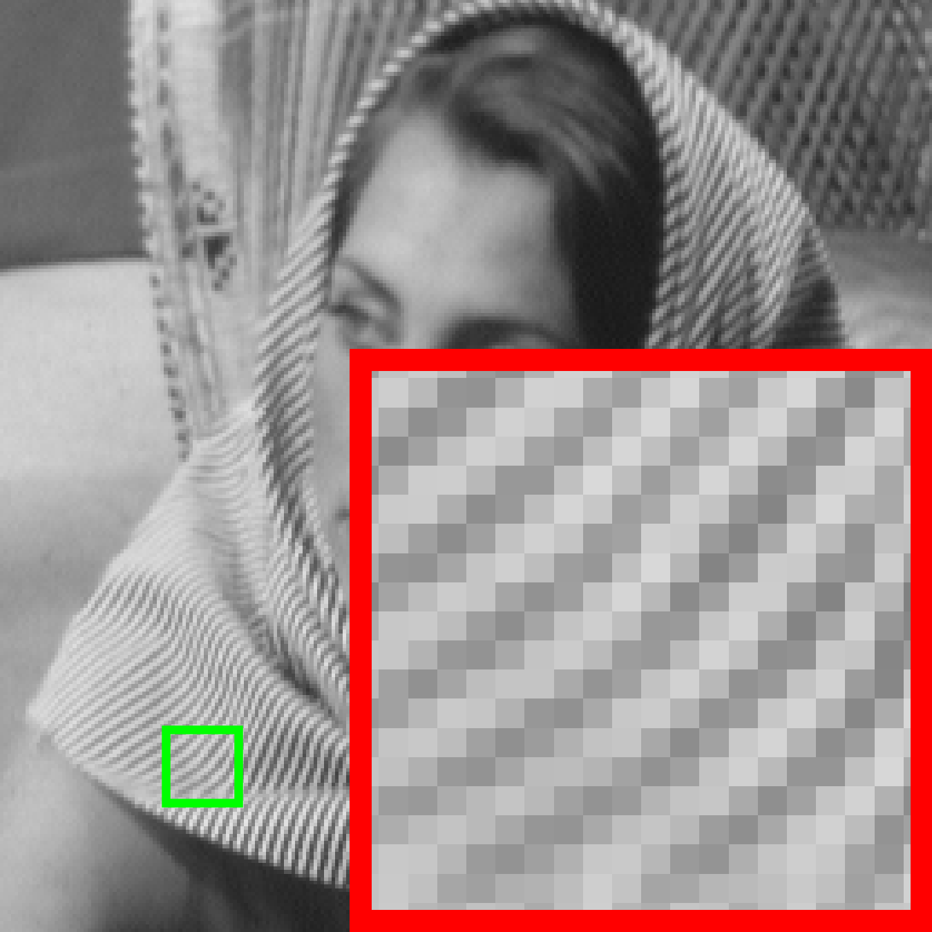
PSNR/SSIM	22.56/0.6260	23.52/0.6940	24.41/0.7249	24.43/0.7264	24.73/0.7674	24.61/0.7691

MADUN	DGUNet+	FSOINet	CASNet	TransCS	PRL-PGD+	IDM (Ours)
25.14/0.7816	26.13/0.8145	25.25/0.7835	25.04/0.7809	24.92/0.7672	28.44/0.8747	32.78/0.9379

Ground Truth	ReconNet	ISTA-Net+	CSNet+	SCSNet	OPINE-Net+	COAST
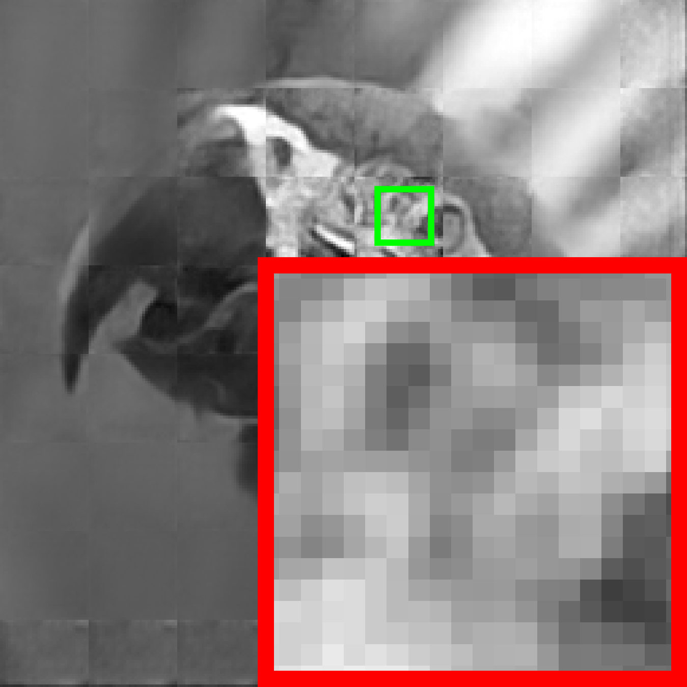
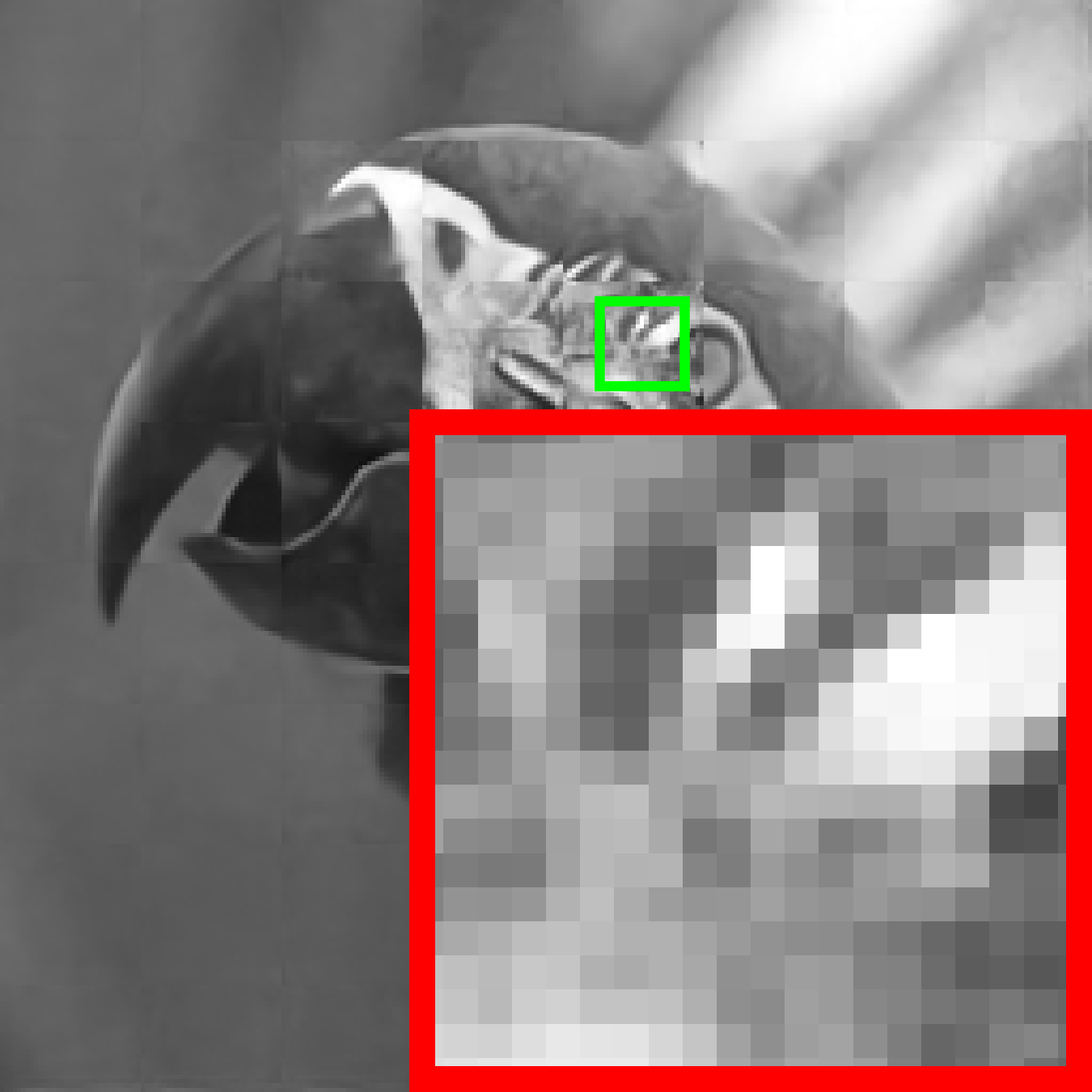
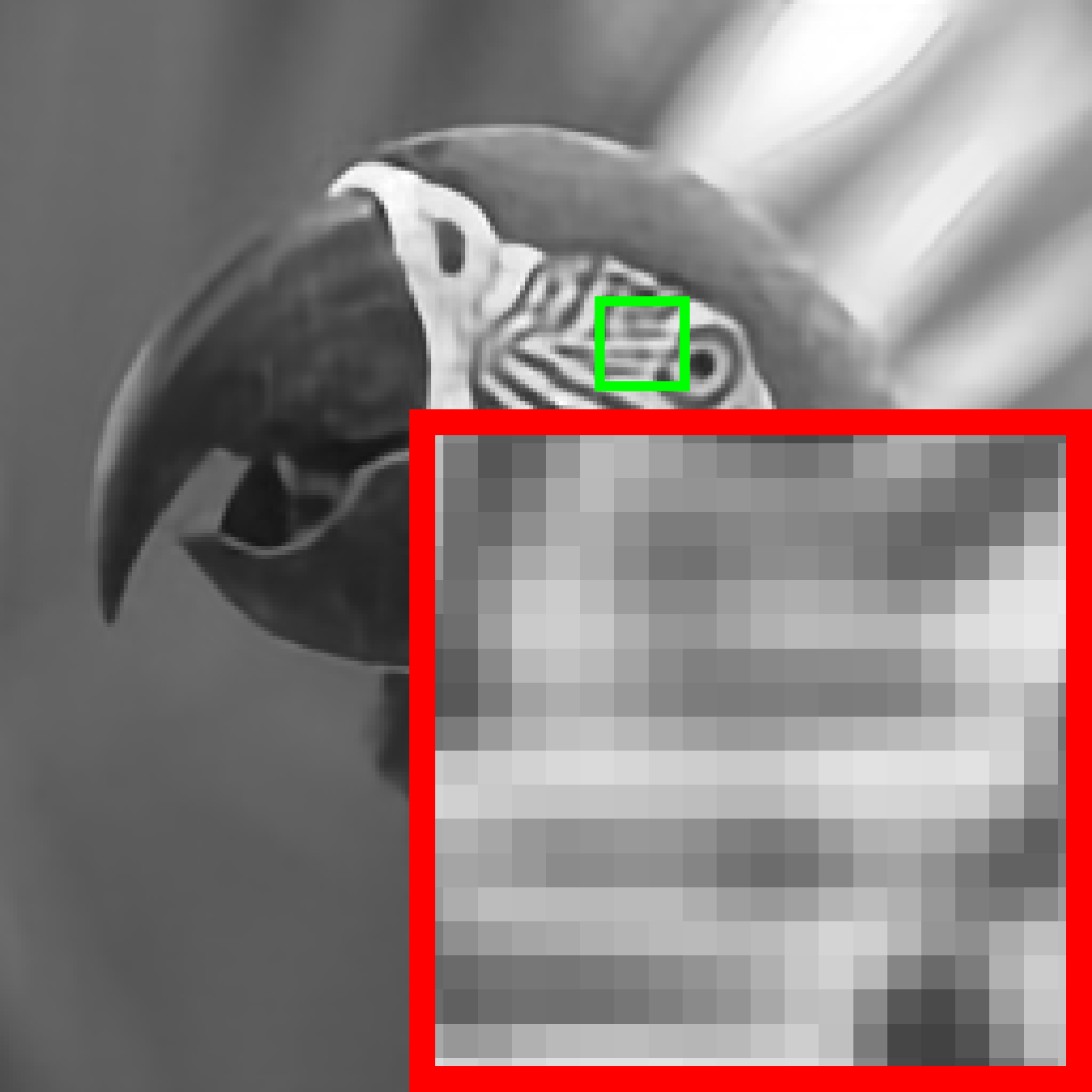
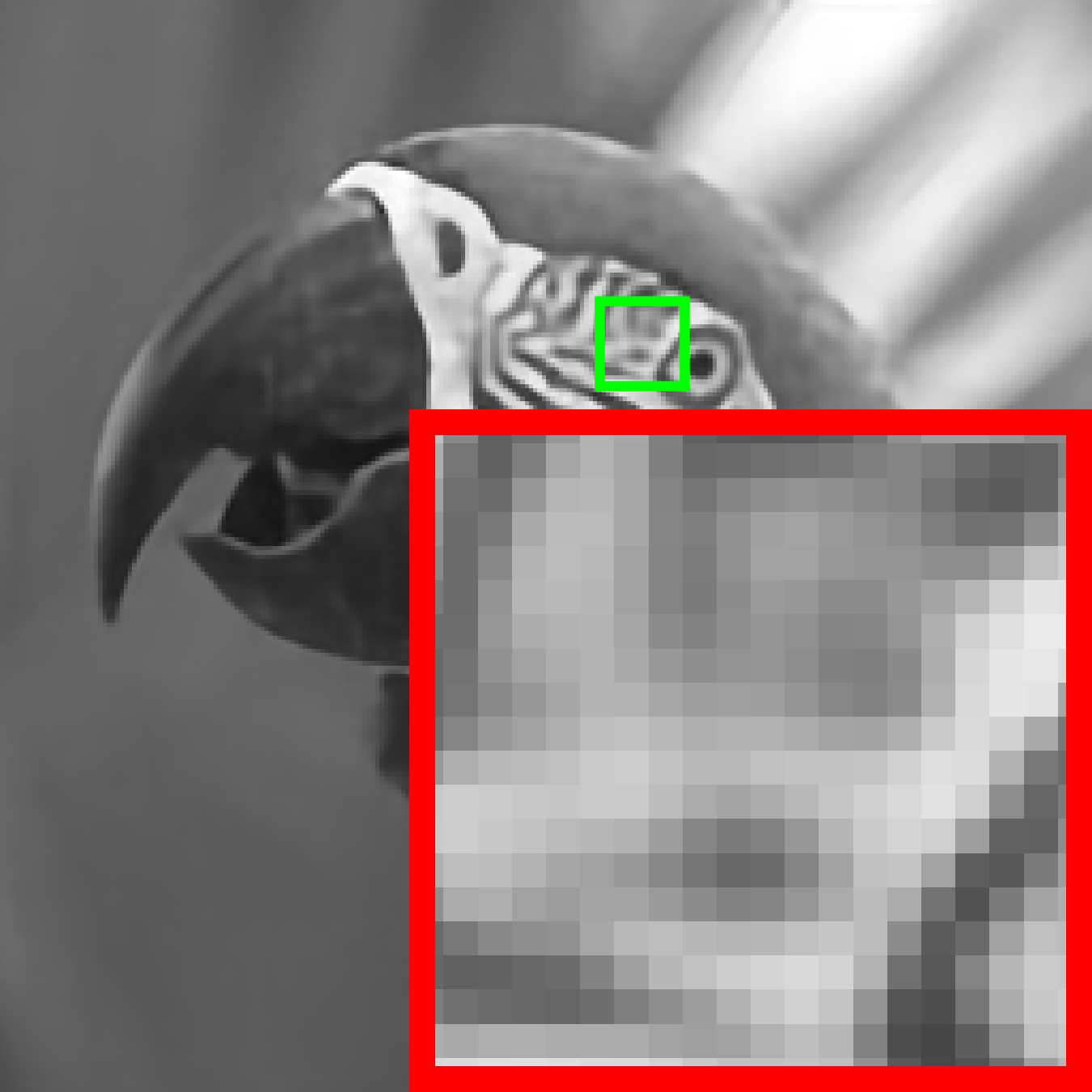
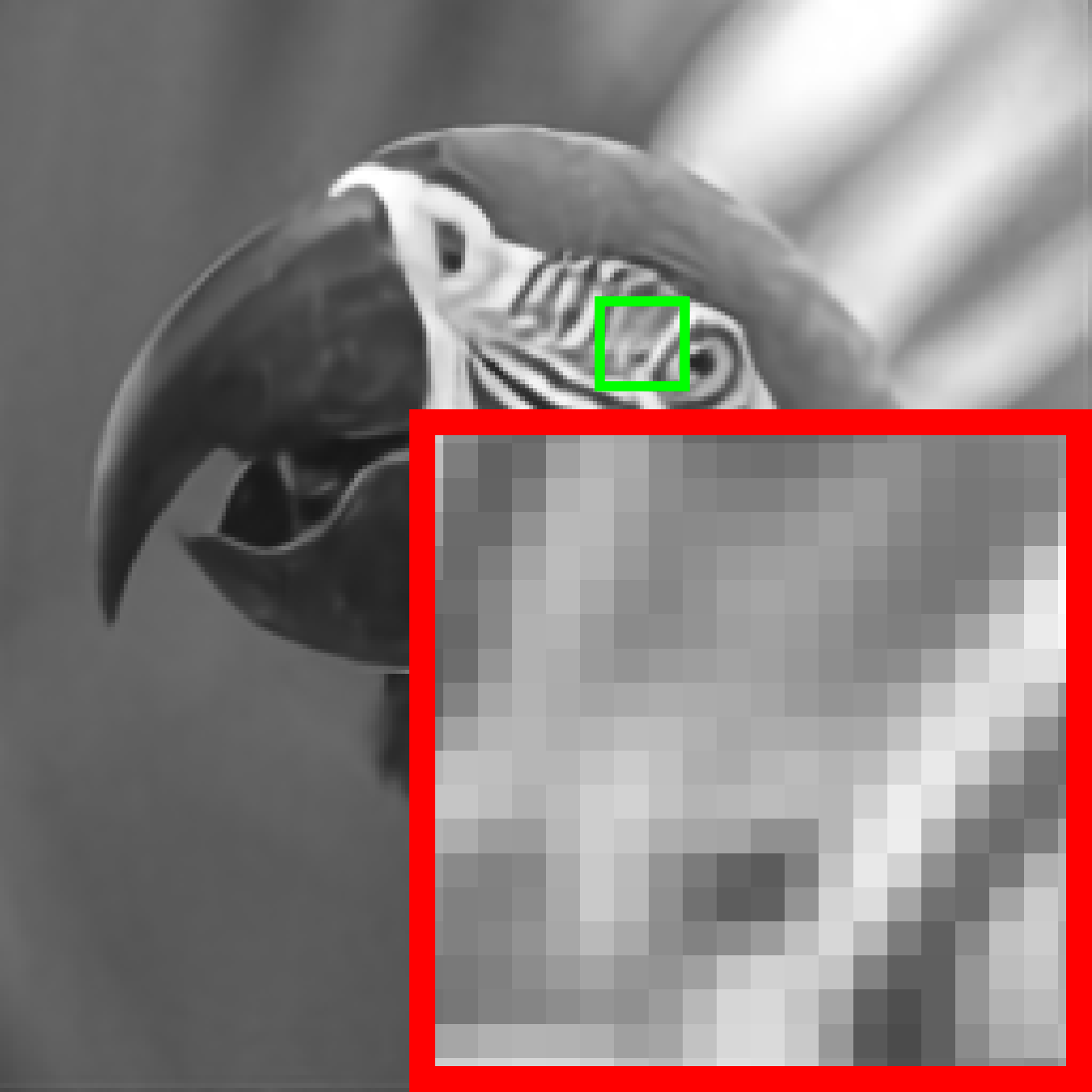
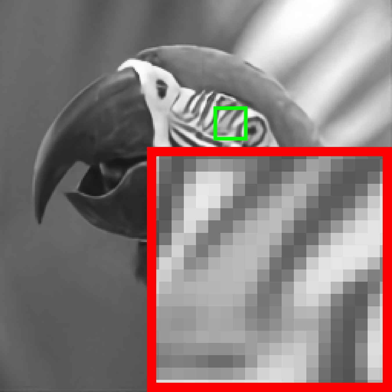
PSNR/SSIM	24.21/0.7660	26.37/0.8523	28.11/0.8899	28.10/0.8921	29.34/0.9155	29.30/0.9206

MADUN	DGUNet+	FSOINet	CASNet	TransCS	PRL-PGD+	IDM (Ours)
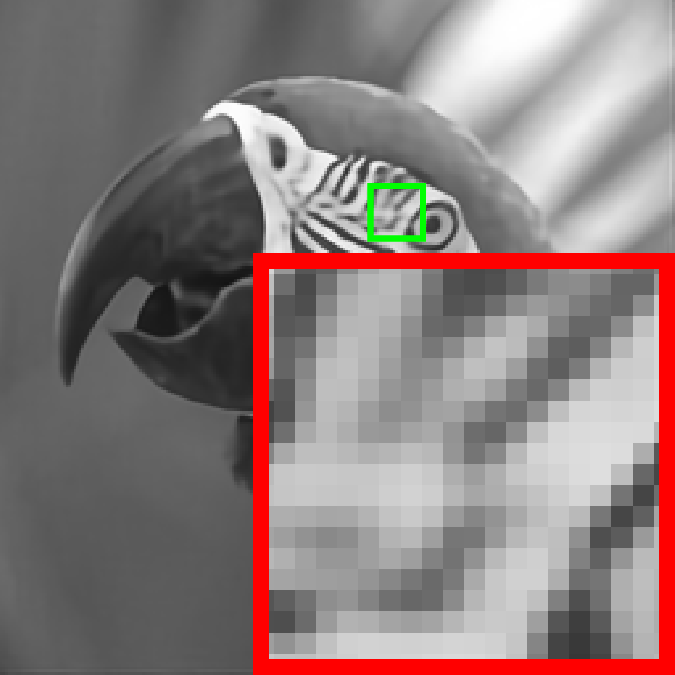
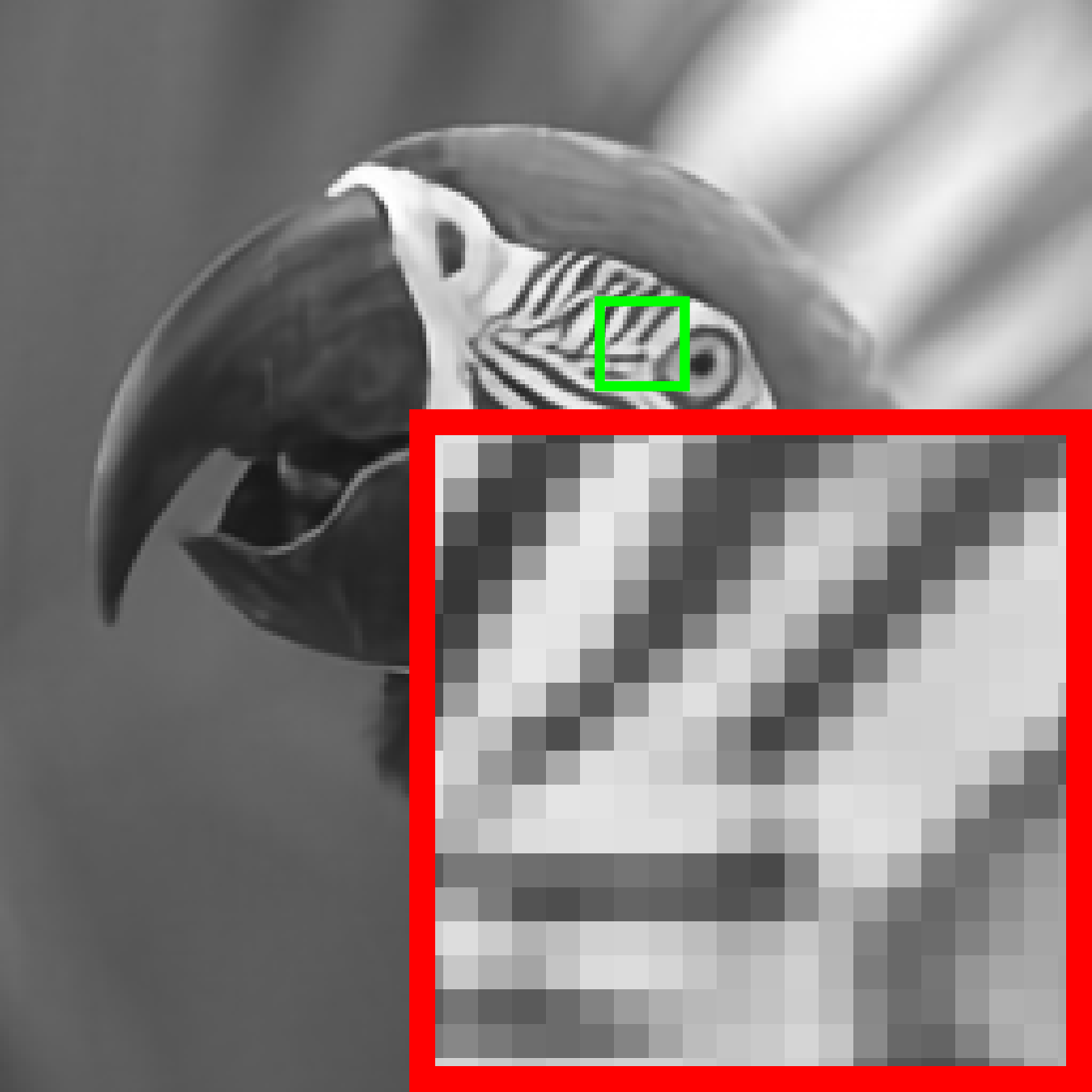
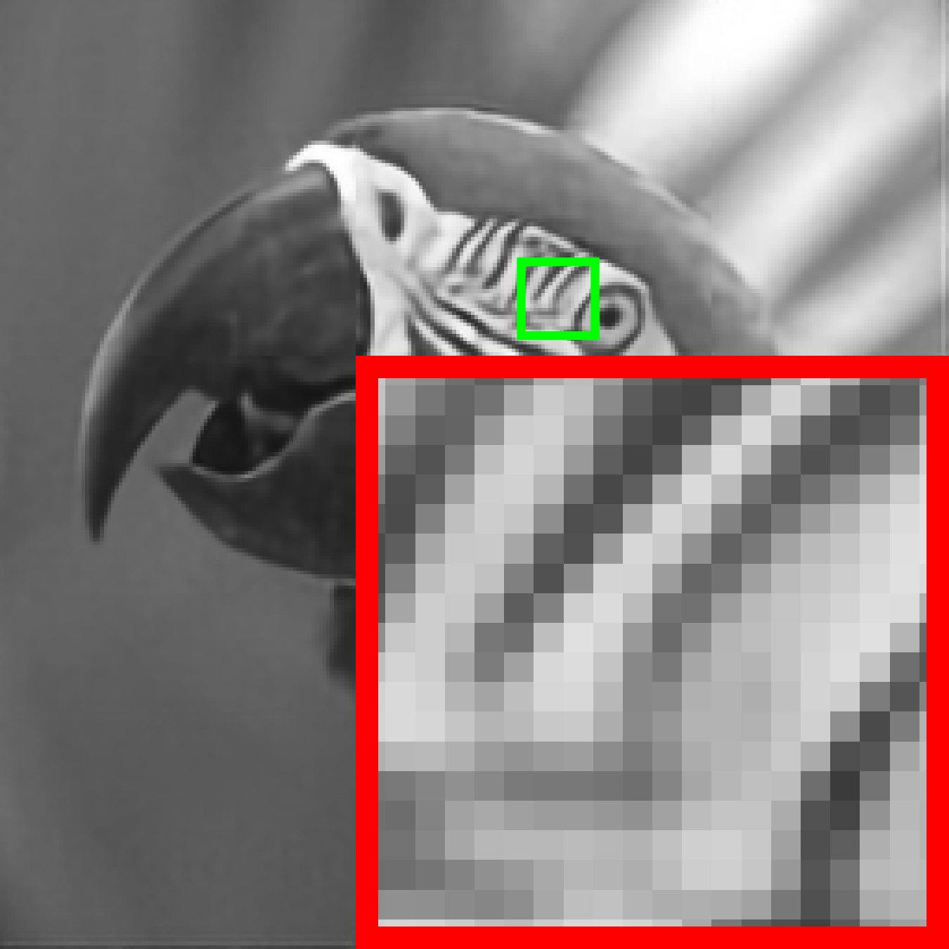
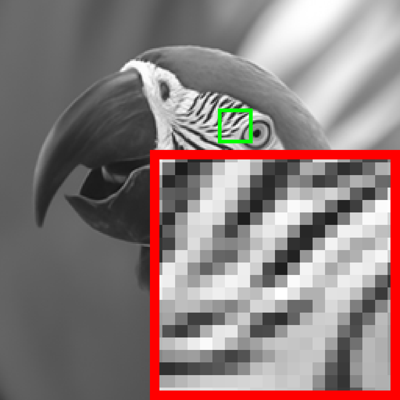
29.46/0.9207	29.75/0.9226	29.81/0.9253	29.71/0.9253	29.44/0.9137	30.81/0.9303	34.85/0.9338

Figure 10: Comparison of CS reconstruction results on the “barbara” (top) and “Parrots” (bottom) images from Set11 at $\gamma=10\%$.

B.2 Application of Our Method to More Tasks

As Tab. 6 reports, we apply IDM to three inverse imaging tasks: inpainting, accelerated MRI, and sparse-view CT, following the setups of previous works (Sun et al., 2016; Chen et al., 2022a). This application involves 4 hours of finetuning and achieves 0.95-5.87dB PSNR enhancements on the previous paradigm of DDNM. As Fig. 12 depicts, IDM improves visual quality in the regions of building appearance, signboard patterns, and human body. These results confirm the generality and consistent efficacy of our method.

Table 6: Average PSNR (dB) for variants (1) and (9) from Tab. 3, extended to three tasks: (i) inpainting on Urban100/DIV2K with 90% pixels randomly dropped, (ii) accelerated MRI on 50 brain images (Sun et al., 2016) at $\gamma=10\%$, and (iii) sparse-view CT on the CT100 dataset (Clark et al., 2013) with 10 views (or angles).

Method Variant		Inpainting	CS-MRI	Sparse-View CT	NFEs ($\downarrow$)
(1)	DDNM (w/o E2E)	20.29/23.03	33.92	30.84	100
(9)	IDM (Ours)	26.16/27.38	36.47	31.79	2

Table 7: Comparison of FID ($\downarrow$)/LPIPS ($\downarrow$) across various diffusion model-based methods on three-channel RGB benchmark images.

	Test Set	Urban100 (100 RGB images of size $256\times 256$)			DIV2K (100 RGB images of size $256\times 256$)
Method	CS Ratio $\gamma$	10%	30%	50%	10%	30%	50%
DDRM (NeurIPS 2022) (Graikos et al., 2022)		184.95/0.4844	50.71/0.1495	21.76/0.0690	264.46/0.5428	93.66/0.2484	39.78/0.1211
$\Pi$GDM (ICLR 2023) (Song et al., 2023c)		209.43/0.4873	108.90/0.2650	76.93/0.1928	254.26/0.5322	165.39/0.3511	134.47/0.2809
DPS (ICLR 2023) (Chung et al., 2023a)		313.62/0.6876	281.52/0.6238	271.42/0.5838	317.67/0.6797	300.14/0.6355	299.35/0.6090
DDNM (ICLR 2023) (Wang et al., 2023c)		212.84/0.5208	56.60/0.2001	23.74/0.1067	269.37/0.5638	111.64/0.3143	52.42/0.1819
GDP (CVPR 2023) (Fei et al., 2023)		211.52/0.4636	118.38/0.3005	88.00/0.2383	202.66/0.4142	116.52/0.2894	95.81/0.2448
PSLD (NeurIPS 2023) (Rout et al., 2023b)		263.62/0.5749	157.69/0.3805	128.81/0.3277	258.68/0.5768	191.54/0.4259	164.17/0.3676
SR3 (TPAMI 2023) (Saharia et al., 2023)		210.77/0.4493	144.52/0.3406	103.67/0.2724	255.78/0.5024	193.18/0.4116	160.33/0.3548
IDM (Ours, $T=3$)		42.72/0.1253	15.46/0.0566	6.47/0.0296	75.44/0.1997	27.29/0.0886	10.69/0.0432

Ground Truth	${\mathbf{A}}^{\dagger}{\mathbf{y}}$	DDRM	$\Pi$GDM	DPS	DDNM	GDP	PSLD	SR3	IDM (Ours)
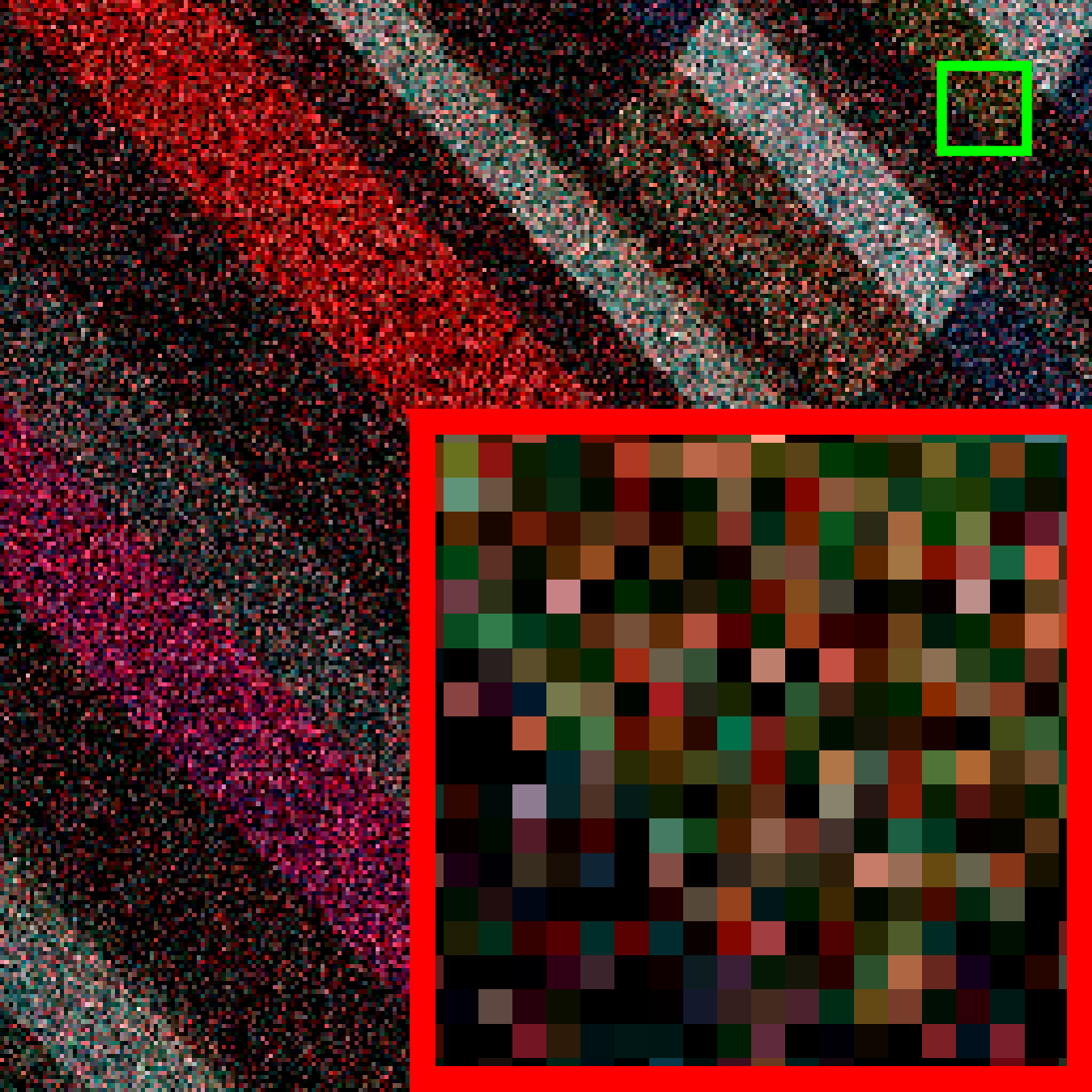
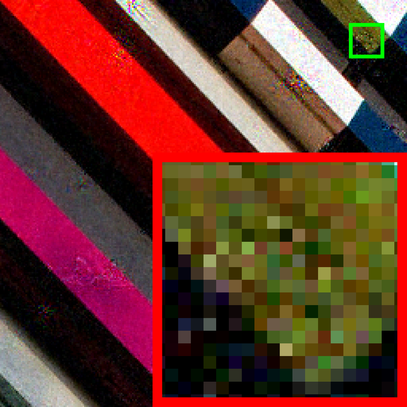
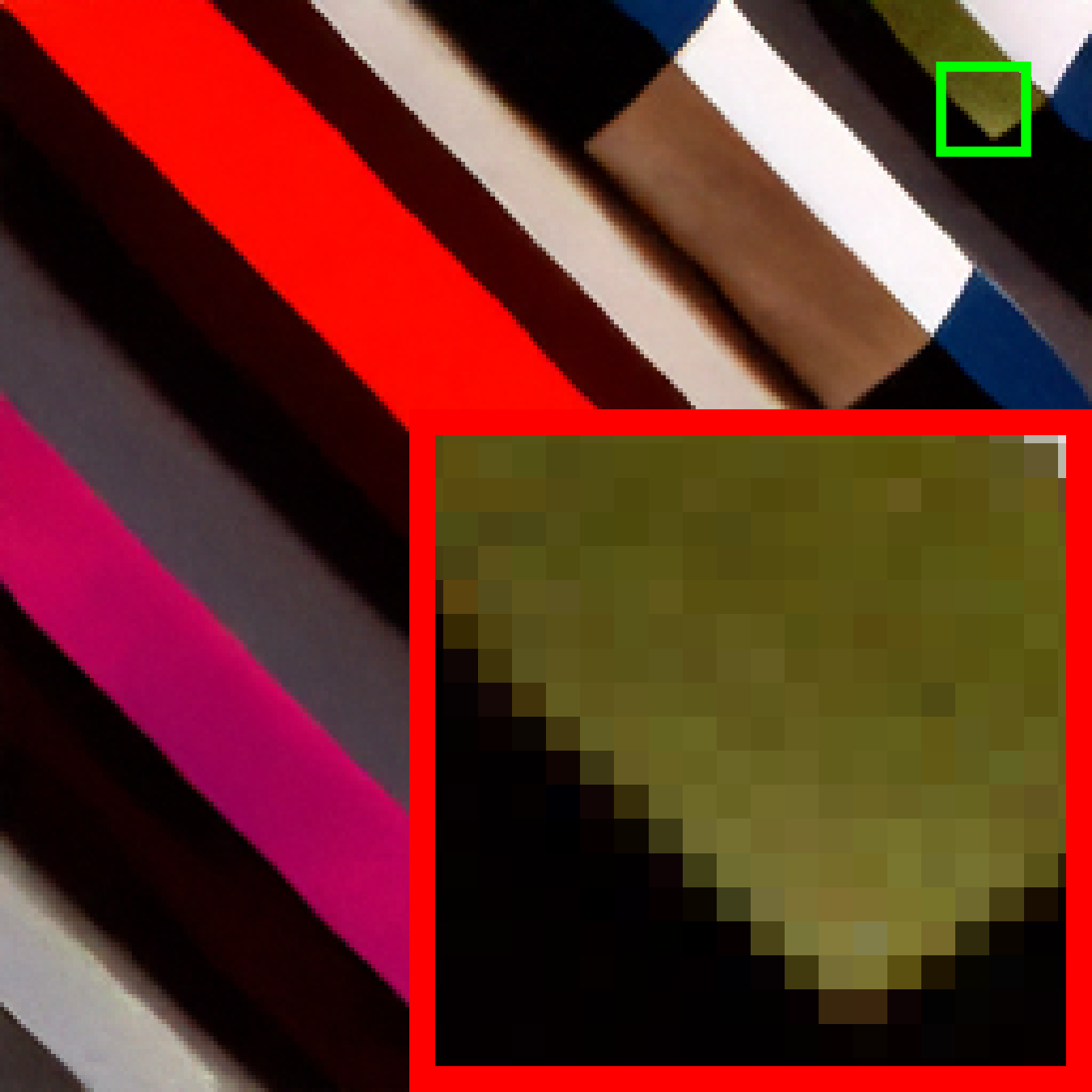
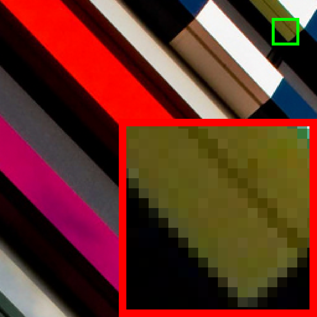
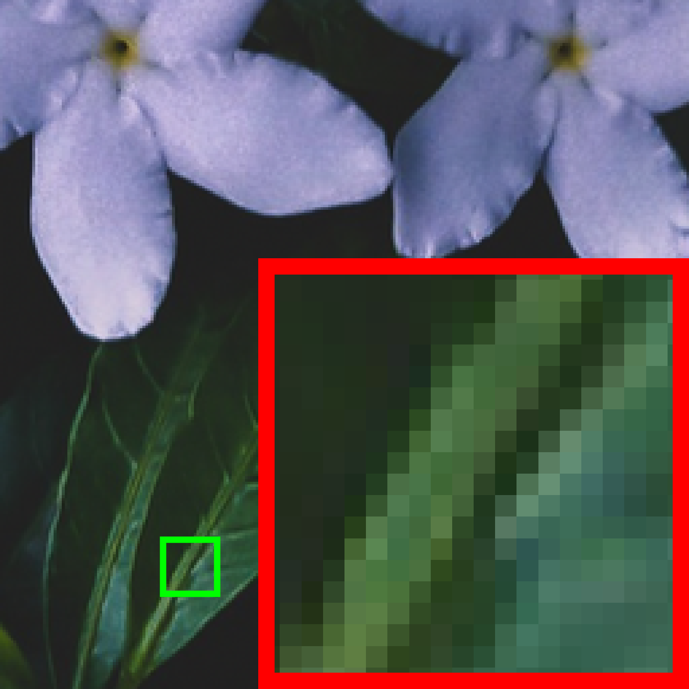
PSNR/SSIM	11.73/0.1015	40.29/0.9617	37.74/0.9459	29.55/0.8405	42.26/0.9684	27.94/0.6550	30.60/0.8905	27.76/0.8273	46.83/0.9895

Ground Truth	${\mathbf{A}}^{\dagger}{\mathbf{y}}$	DDRM	$\Pi$GDM	DPS	DDNM	GDP	PSLD	SR3	IDM (Ours)
PSNR/SSIM	12.79/0.0768	39.66/0.9581	35.85/0.9292	27.71/0.8150	40.72/0.9562	29.74/0.7529	28.18/0.9025	27.65/0.8151	52.17/0.9969

Figure 11: Comparison of CS reconstruction results on “img_081” from Urban100 (top) and “0877” from DIV2K (bottom) at $\gamma=50\%$.

Ground Truth	Measurement	(1) DDNM	(9) Ours	Ground Truth	Measurement	(1) DDNM	(9) Ours
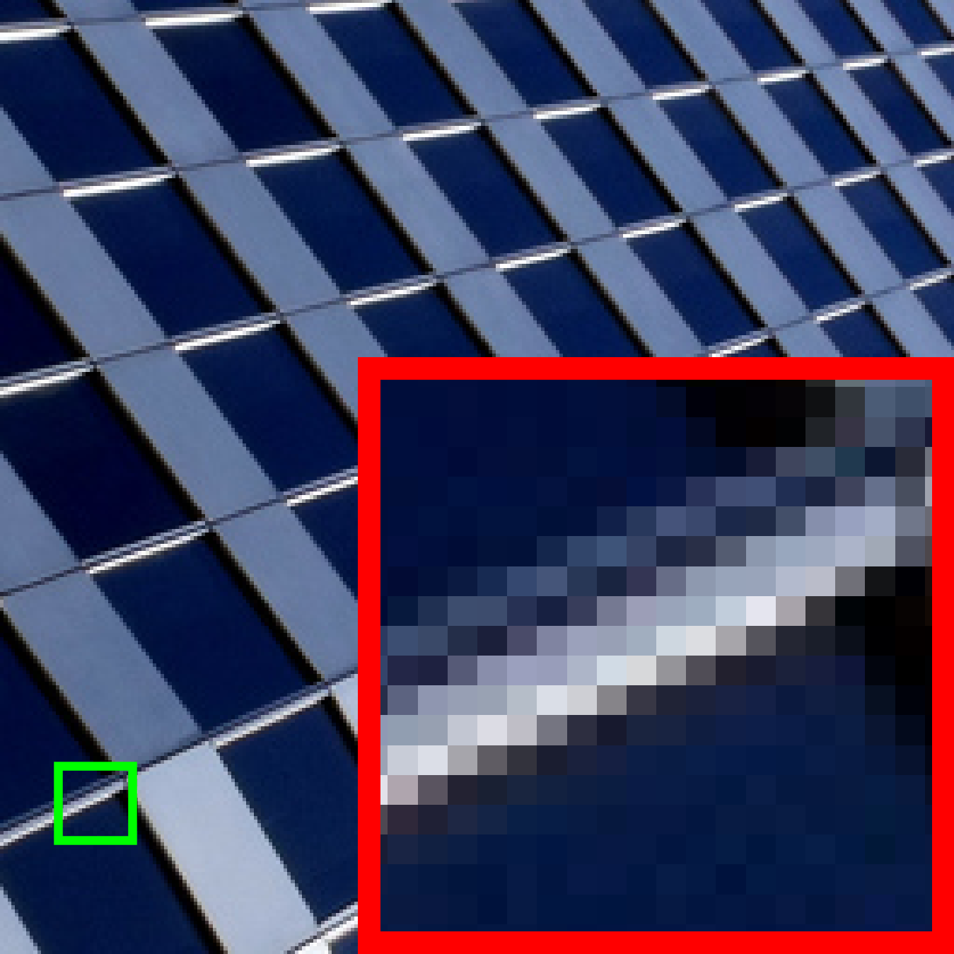
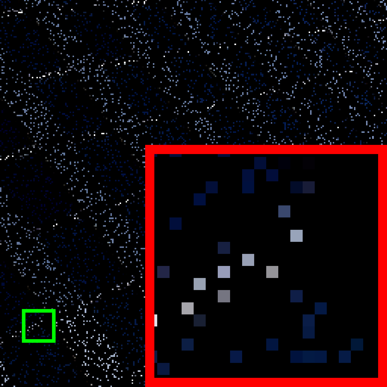
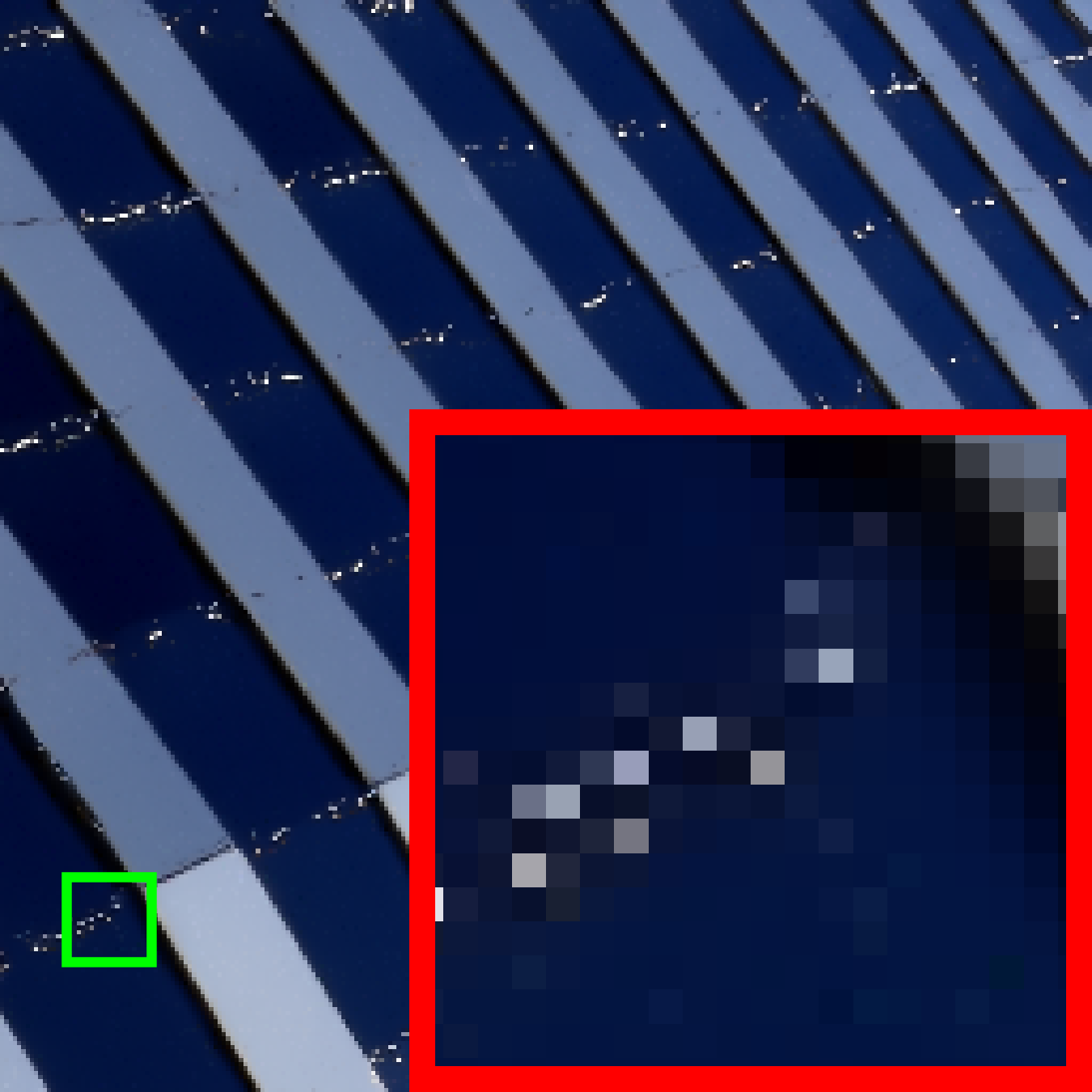
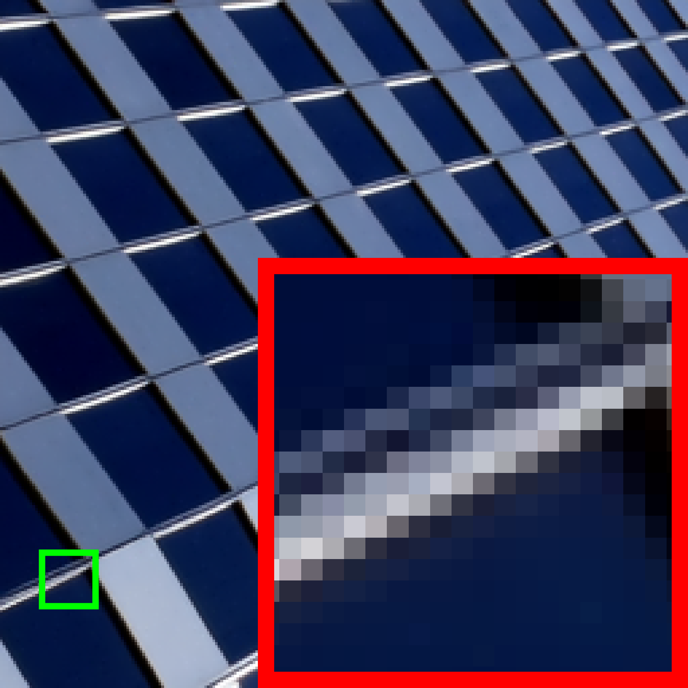
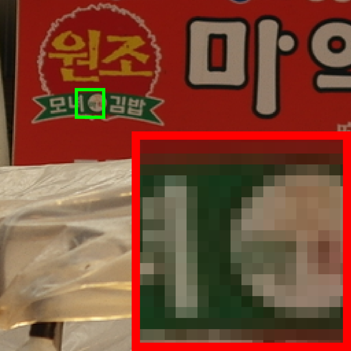
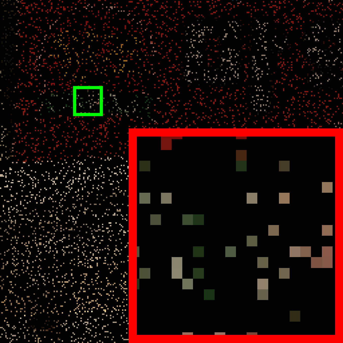
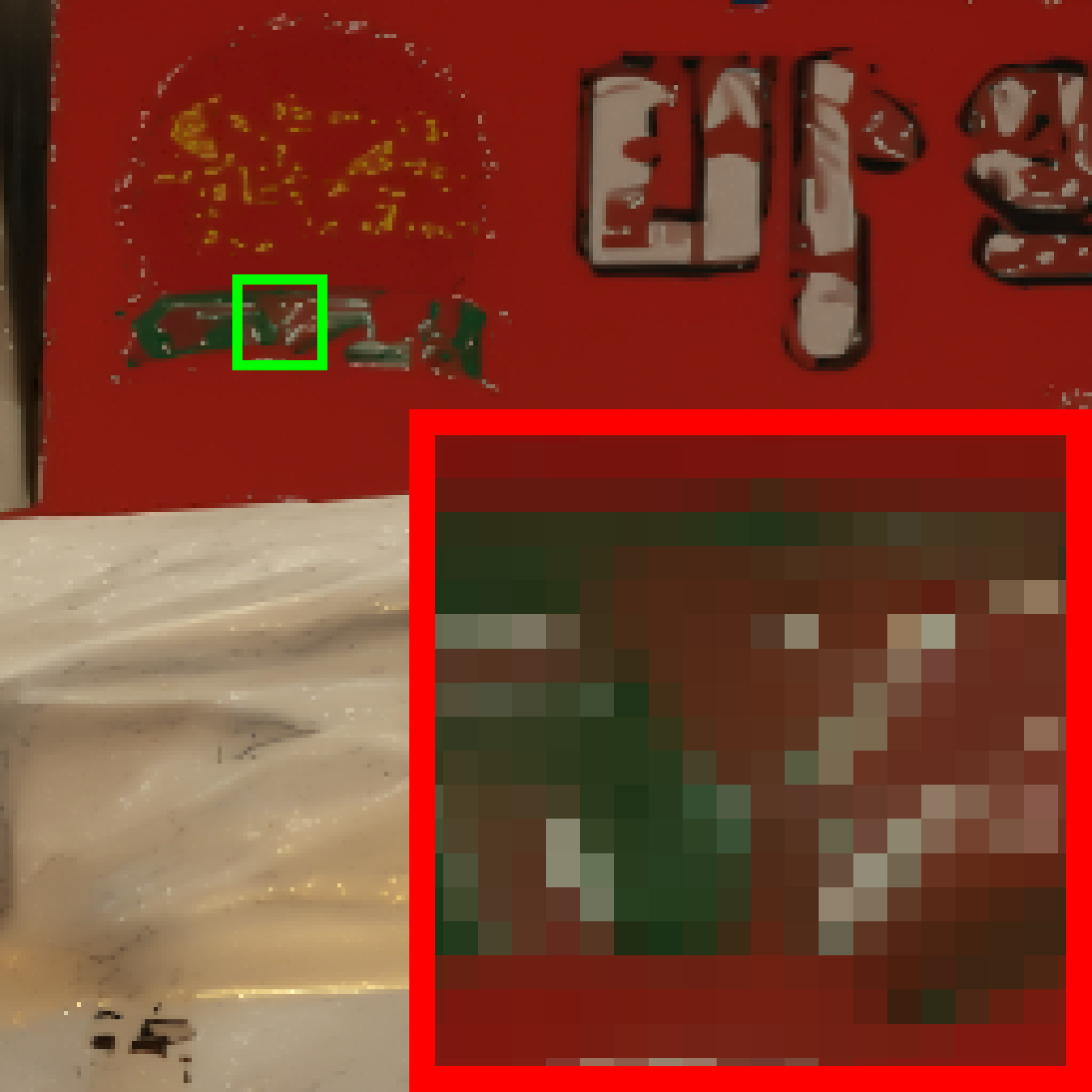
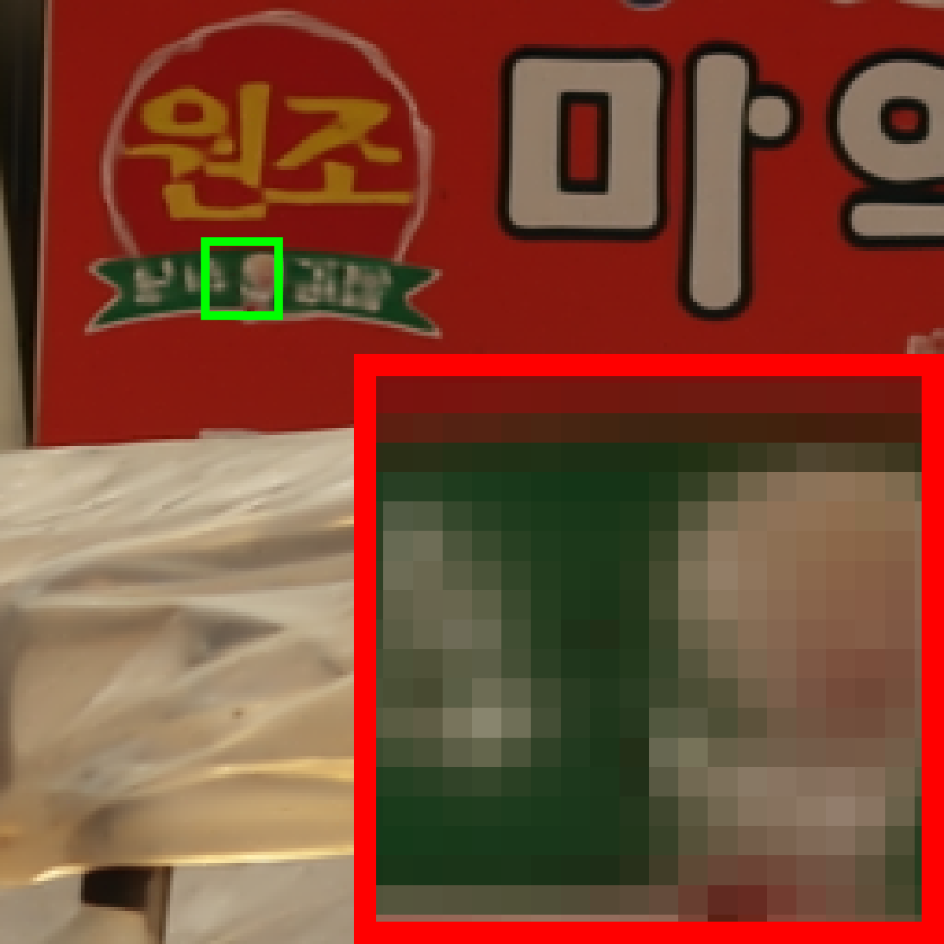
PSNR/SSIM	7.23/0.0789	18.12/0.8027	31.49/0.9707	PSNR/SSIM	6.91/0.0346	22.79/0.7611	31.40/0.9268

Ground Truth	Zero-Filling	(1) DDNM	(9) Ours	Ground Truth	FBP	(1) DDNM	(9) Ours
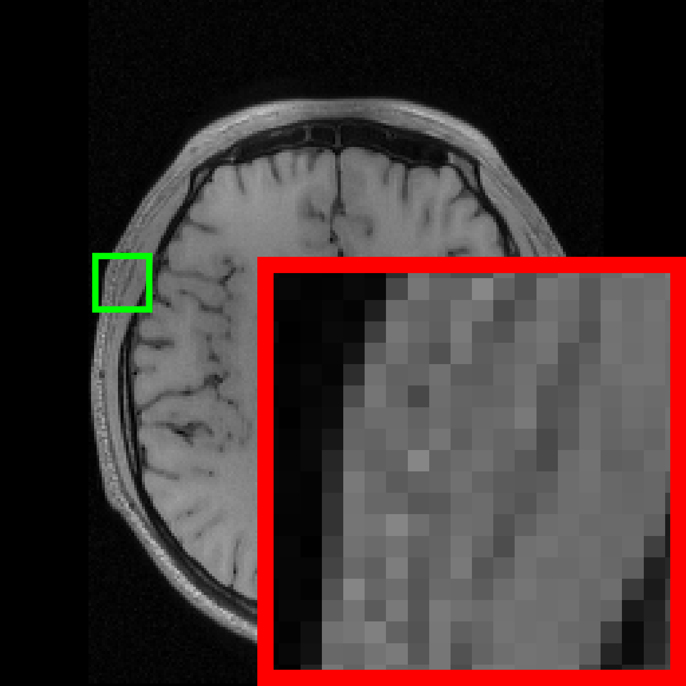
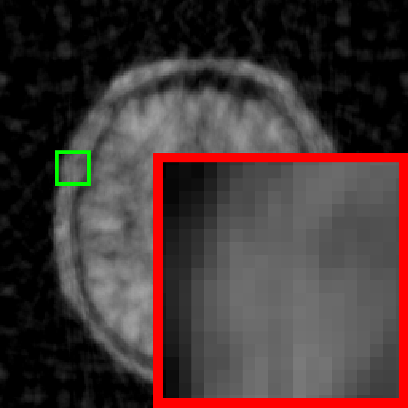
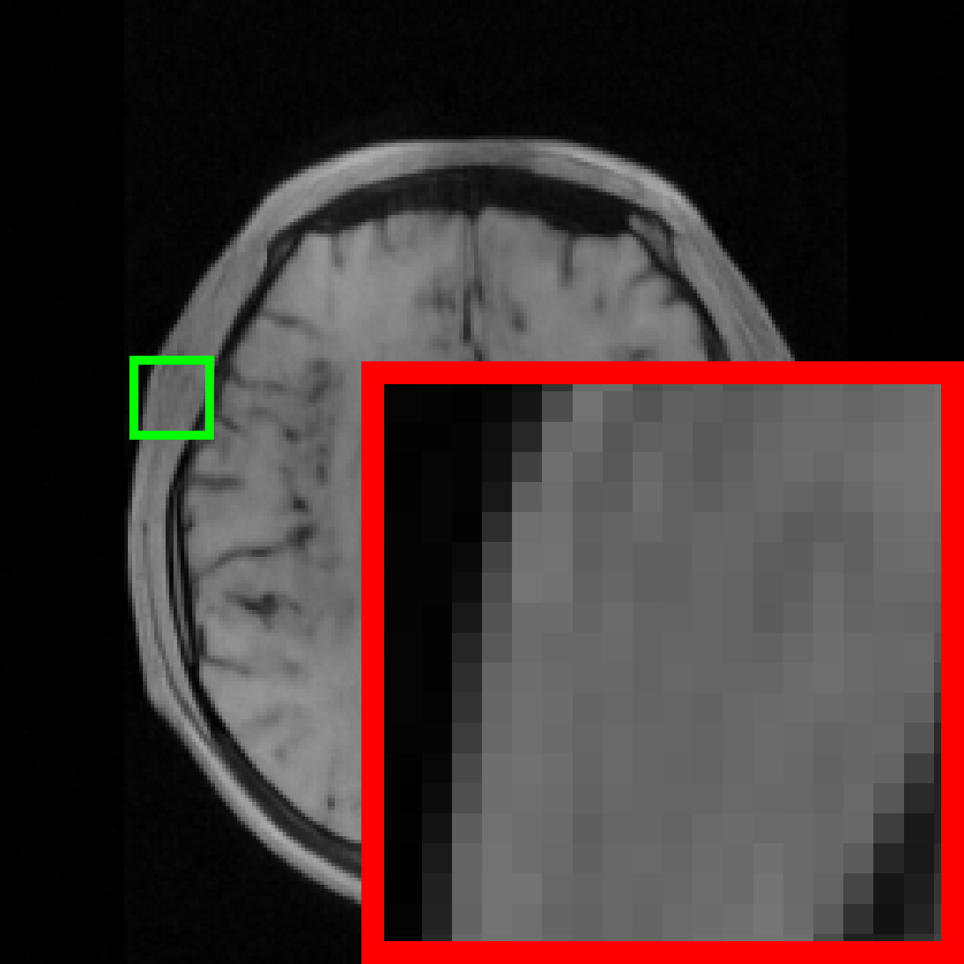
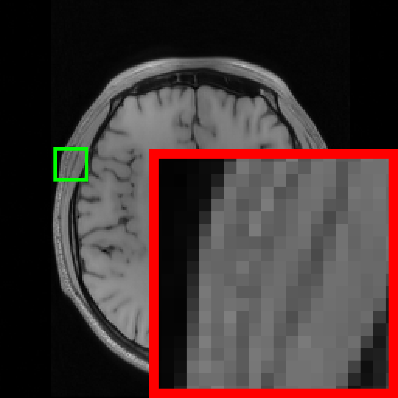
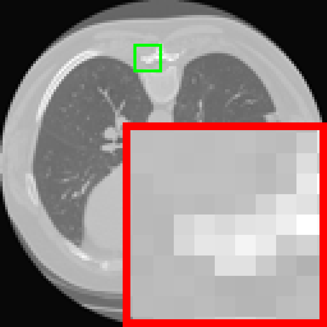
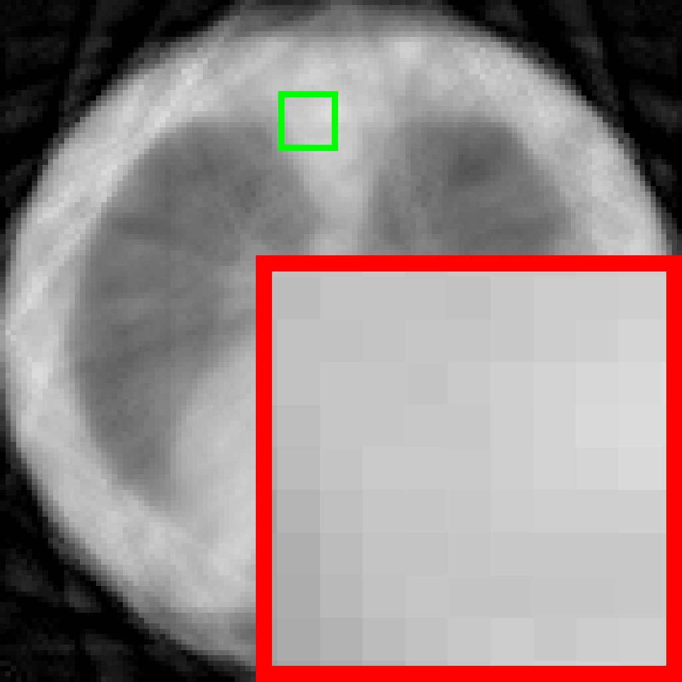
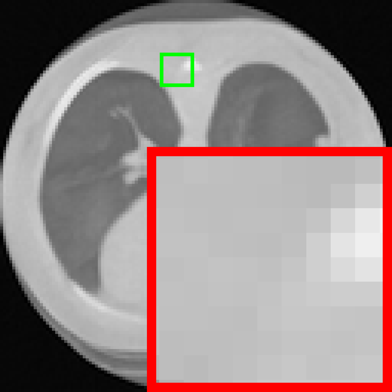
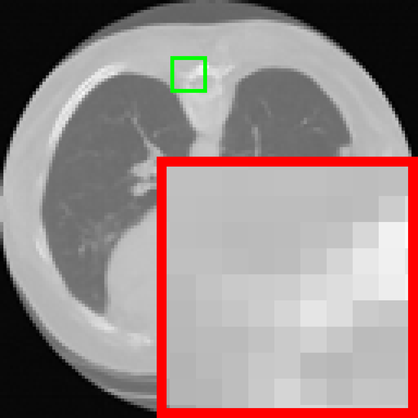
PSNR/SSIM	23.65/0.5137	31.60/0.8901	35.71/0.9438	PSNR/SSIM	23.55/0.5977	30.47/0.8688	32.40/0.9032

Figure 12: Comparison of recovery results from variants (1) and (9) in Tab. 3, evaluated on three tasks of inpainting on Urban100 (top left) and DIV2K (top right), CS-MRI (bottom left), and sparse-view CT (bottom right). Average PSNR results are presented in Tab. 6.

B.3 Visualization of Intermediate Recovery Results

Figs. 13 and 14 display the intermediate results of DDNM (Wang et al., 2023c, b) ($T=1000$ with 100 NFEs) and our IDM ($T=3$ with 3 NFEs) in RGB image CS and inpainting tasks. The figures illustrate the intermediate predictions ${\bar{\mathbf{x}}}_{0|t}$ at various diffusion sampling steps. Although in this experiment, both two methods utilize the same U-Net of SD v1.5, finetuned on the identical dataset, our IDM not only yields higher quality and more accurate reconstruction results, with about a 5-7dB lead in PSNR, but also requires much fewer steps/NFEs. Notably, our IDM achieves a 98.9% reduction in inference time (from 86.91s to 0.98s) on DDNM. These results verify the efficacy of our end-to-end CS learning.

In addition, we highlight that the intermediate results ${\bar{\mathbf{x}}}_{0|t}$ in Figs. 13 and 14 from our end-to-end finetuned IDM enjoy a certain degree of interpretability: they retain the characteristics of images without any additional processing and do not devolve into overly abstract or indecipherable feature maps. These intermediate results display a consistent trend of improved PSNR and SSIM scores, marked by their progressively reduced distortion, enhanced detail and texture accuracy, and steadily increasing visual quality.

Ground Truth	${\mathbf{A}}^{\dagger}{\mathbf{y}}$	IDM (Ours, 1 Step)	IDM (Ours, 2 Steps)	IDM (Ours, 3 Steps)
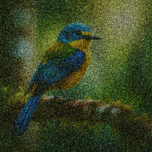
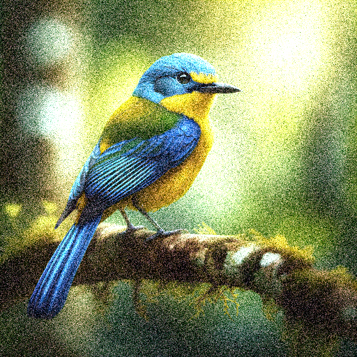
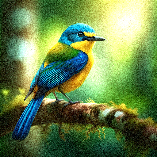
PSNR/SSIM	10.99/0.0626	13.40/0.1486	19.46/0.3047	35.26/0.8991

DDNM (20 Steps)	DDNM (40 Steps)	DDNM (60 Steps)	DDNM (80 Steps)	DDNM (100 Steps)
14.23/0.1257	22.96/0.4302	28.56/0.6720	29.42/0.6846	30.27/0.7295

Figure 13: Visual comparison of intermediate results in CS reconstruction by DDNM (Wang et al., 2023c, b) and our IDM based on the U-Net of SD v1.5 (Rombach et al., 2022) on a $512\times 512$ RGB image at a CS ratio of $\gamma=30\%$. Please zoom in for optimal viewing.

Measurement	DDNM (20 Steps)	DDNM (40 Steps)	DDNM (60 Steps)	DDNM (80 Steps)	DDNM (100 Steps)	IDM (Ours, 1 Step)	IDM (Ours, 2 Steps)	IDM (Ours, 3 Steps)
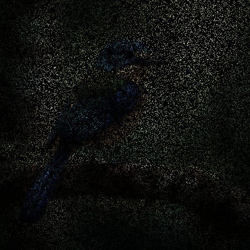
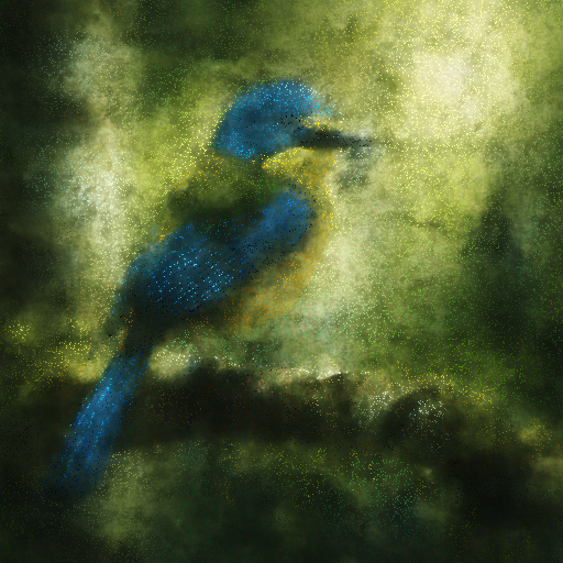
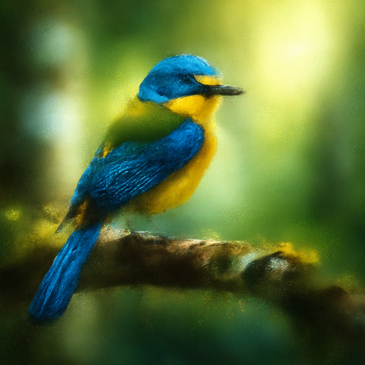
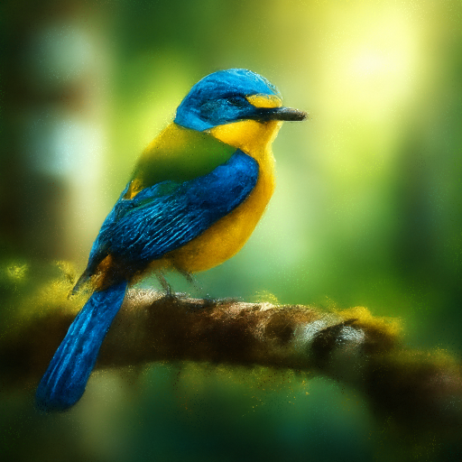
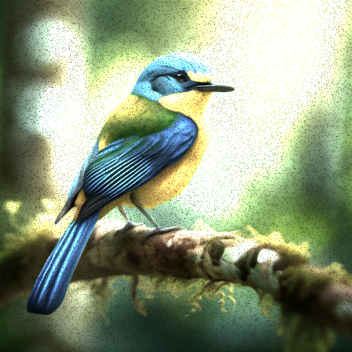
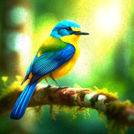
7.32/0.0714	17.67/0.4568	21.24/0.6202	23.74/0.7482	24.89/0.8050	25.24/0.8273	11.64/0.3330	16.49/0.5614	32.64/0.9480

Figure 14: Visual comparison of intermediate results in inpainting by DDNM and our IDM with 90% image pixels randomly masked.

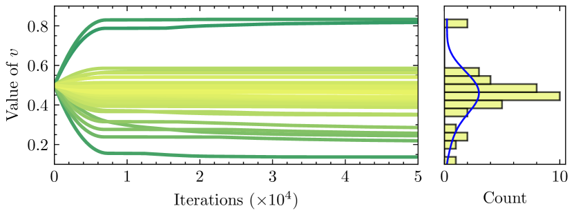
Figure 15: Analysis of our introduced 43 different $v$ values in IDM ($T=3$) for RGB image CS task at $\gamma=10\%$. The left subgraph presents the evolution curves of these $v$ values, and the right subgraph displays the distribution of final learned values.

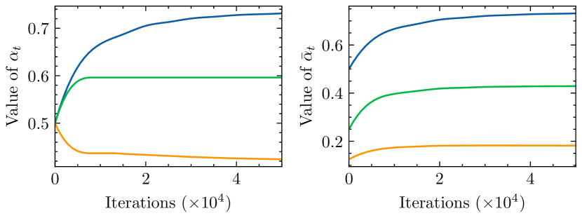
Figure 16: Analysis of our learned $\alpha$ values in the same IDM from Fig. 15. The left subgraph dipicts evolution of $\{\alpha_{1},\alpha_{2},\alpha_{3}\}$. The right graph further shows progression of $\{\bar{\alpha}_{1},\bar{\alpha}_{2},\bar{\alpha}_{3}\}~{}(\bar{\alpha}_{t}=\prod_{i=0}^{t}\alpha_{i})$. The blue (top), green (middle), and orange (bottom) curves represent the step indices $t$ of 1, 2, and 3, respectively.

B.4 Analysis of Learned Parameters $\{v\}$, $\{\alpha\}$, and $\{w\}$

Tab. 5 evaluates IDM variants with different $v$ initialization values from 0.1 to 1.0. We observe that a reduction in $v_{t}$ from the default 0.5 to 0.4 enhances performance by 0.12dB in PSNR. This indicates that higher $v$ values could overly change the pre-defined diffusion sampling process and NN architecture, reducing the advantage of using pre-trained U-Net weights for finetuning. Such an effect is further evident as the performance of IDM drops with $v$ value going greater than 0.5. Conversely, a slightly smaller $v$ value can bring minor modifications to pre-trained features, thus leading to better initializations. However, as $v$ approaches zero, the numerical errors in the multiple stacked wired layers related to the second pathway of auxiliary variable ${\mathbf{h}}$ will increase. This leads to less precise recomputations for inputs, intermediate features, and gradients, with performance drops. We also experiment with $u$ and $v$ as free parameters initialized to 0.5 without constraining $u+v\equiv 1$, and another IDM variant fixing $u=v\equiv 0.5$. These two modifications lead to PSNR decreases of 0.15dB and 0.20dB, respectively.

We provide additional results about the learnable parameters $v$, $\alpha$, and $w$ during training. Fig. 15 displays the progression of 43 $v$ values in our various wired invertible layers, as formulated in Eqs. (4) and (5). Starting from 0.5, these $v$ values converge to their respective final numbers, forming a distribution akin to a normal curve with a mean of 0.45 and a standard deviation of 0.13. Fig. 16 exhibits that all $\alpha$ values initialized to 0.5 follow different trajectories: $\alpha_{1}$, $\alpha_{2}$, and $\alpha_{3}$ increase to 0.73 and 0.59, and decrease to 0.42, respectively, while $\bar{\alpha}_{1}$, $\bar{\alpha}_{2}$, and $\bar{\alpha}_{3}$ converges to 0.73, 0.43, and 0.18. Meanwhile, we observe that $w_{T}$ and $w_{0}$ begin at 1.0 and 0.0, respectively, and gradually increase to 1.46 and 0.21. In contrast to the widely adopted fixed diffusion parameters like the linearly increasing $\beta_{t}~{}(\alpha_{t}=1-\beta_{t})$ values scheduled from 0.0001 to 0.02 (Ho et al., 2020), our learned parameters can enjoy increased adaptability and optimization freedom for CS. Further analysis and interpretation of these learned values will be pursued in our future work.

Table 8: PSNR Comparison on Set11 at $\gamma=10\%$ for end-to-end IDM training on a single 1080Ti GPU with 11GB memory.

Method Variant (w/ Our End-to-End Training)	PSNR (dB, $\uparrow$)
Invertible (Ours, $T=2$, Batch Size: $16\times 128^{2}$)	32.18
Non-Invertible (w/ Reduced Batch Size: 2)	31.58 (-0.60)
Non-Invertible (w/ Gradient Accumulation)	32.01 (-0.17)
Non-Invertible (w/ Reduced Patch Size: 32)	29.79 (-2.39)

Table 9: Memory usage comparison on a single 1080Ti GPU.

Method Variant (w/ Our End-to-End Training)	Memory (GB, $\downarrow$)
Invertible (Ours, $T=2$, Batch Size: $8\times 128^{2}$)	6.71
Non-Invertible (w/ Activation Checkpointing)	8.54 (+1.83)

B.5 Effect of Invertible Design for Memory Efficiency

While our invertible design is effective in minimizing memory use, there are other techniques for training non-invertible NNs, including reducing batch sizes, using gradient accumulation, decreasing image patch sizes, and employing activation checkpointing (Mangalam et al., 2022). This subsection evaluates the performance/efficiency of these techniques and confirms the feasibility of IDMs for consumer-grade GPUs.

We conduct experiments using scaled-down IDM variants for luminance component CS on a GTX 1080Ti GPU with 11GB memory. Tab. 8 compares our IDM with three non-invertible model variants. We observe that reducing batch size from 16 to 2 leads to a 0.60dB decrease in PSNR, applying gradient accumulation results in a 0.17dB reduction and triples training time, while decreasing the patch size from 128 to 32 causes a significant performance drop of 2.39dB.

Moreover, Tab. 9 compares the memory of IDM and a non-invertible variant using activation checkpointing. We observe that our IDM with a two-level invertible design is more memory-efficient, reducing usage by 21.43% compared to the activation checkpointing-based method. These results validate the effectiveness and practicality of our invertible design for finetuning on standard consumer-grade GPUs.

References

- Adler et al. (2017) Adler, A., Boublil, D., and Zibulevsky, M. Block-based compressed sensing of images via deep learning. In 2017 IEEE 19th International Workshop on Multimedia Signal Processing (MMSP), pp. 1–6, 2017. doi: 10.1109/MMSP.2017.8122281.
- Aggarwal et al. (2018) Aggarwal, H. K., Mani, M. P., and Jacob, M. MoDL: Model-based deep learning architecture for inverse problems. IEEE Transactions on Medical Imaging, 38(2):394–405, 2018.
- Agustsson & Timofte (2017) Agustsson, E. and Timofte, R. NTIRE 2017 Challenge on Single Image Super-Resolution: Dataset and Study. In Proceedings of IEEE Conference on Computer Vision and Pattern Recognition Workshops (CVPRW), pp. 126–135, 2017.
- Chen & Zhang (2022) Chen, B. and Zhang, J. Content-aware Scalable Deep Compressed Sensing. IEEE Transactions on Image Processing, 31:5412–5426, 2022.
- Chen et al. (2023a) Chen, B., Song, J., Xie, J., and Zhang, J. Deep Physics-Guided Unrolling Generalization for Compressed Sensing. International Journal of Computer Vision, 131(11):2864–2887, 2023a.
- Chen & Davies (2020) Chen, D. and Davies, M. E. Deep Decomposition Learning for Inverse Imaging Problems. In Proceedings of European Conference on Computer Vision (ECCV), pp. 510–526, 2020.
- Chen et al. (2022a) Chen, D., Tachella, J., and Davies, M. E. Robust Equivariant Imaging: a Fully Unsupervised Framework for Learning to Image from Noisy and Partial Measurements. In Proceedings of IEEE Conference on Computer Vision and Pattern Recognition (CVPR), pp. 5647–5656, 2022a.
- Chen et al. (2008) Chen, G.-H., Tang, J., and Leng, S. Prior Image Constrained Compressed Sensing (PICCS): A Method to Accurately Reconstruct Dynamic CT Images from Highly Undersampled Projection Data Sets. Medical Physics, 35(2):660–663, 2008.
- Chen et al. (2020) Chen, J., Sun, Y., Liu, Q., and Huang, R. Learning Memory Augmented Cascading Network for Compressed Sensing of Images. In Proceedings of European Conference on Computer Vision (ECCV), pp. 513–529, 2020.
- Chen et al. (2022b) Chen, W., Yang, C., and Yang, X. FSOINet: Feature-Space Optimization-Inspired Network for Image Compressive Sensing. In Proceedings of IEEE International Conference on Acoustics, Speech and Signal Processing (ICASSP), pp. 2460–2464, 2022b.
- Chen et al. (2021) Chen, Z., Guo, W., Feng, Y., Li, Y., Zhao, C., Ren, Y., and Shao, L. Deep-Learned Regularization and Proximal Operator for Image Compressive Sensing. IEEE Transactions on Image Processing, 30:7112–7126, 2021.
- Chen et al. (2023b) Chen, Z., Zhang, Y., Ding, L., Bin, X., Gu, J., Kong, L., and Yuan, X. Hierarchical integration diffusion model for realistic image deblurring. In Proceedings of Neural Information Processing Systems (NeurIPS), 2023b.
- Cheng et al. (2021) Cheng, Z., Chen, B., Liu, G., Zhang, H., Lu, R., Wang, Z., and Yuan, X. Memory-Efficient Network for Large-Scale Video Compressive Sensing. In Proceedings of IEEE Conference on Computer Vision and Pattern Recognition (CVPR), pp. 16246–16255, 2021.
- Chung et al. (2022) Chung, H., Sim, B., Ryu, D., and Ye, J. C. Improving Diffusion Models for Inverse Problems using Manifold Constraints. In Proceedings of Neural Information Processing Systems (NeurIPS), volume 35, pp. 25683–25696, 2022.
- Chung et al. (2023a) Chung, H., Kim, J., Mccann, M. T., Klasky, M. L., and Ye, J. C. Diffusion Posterior Sampling for General Noisy Inverse Problems. In Proceedings of International Conference on Learning Representations (ICLR), 2023a.
- Chung et al. (2023b) Chung, H., Kim, J., and Ye, J. C. Direct Diffusion Bridge Using Data Consistency for Inverse Problems. In Proceedings of Neural Information Processing Systems (NeurIPS), 2023b.
- Chung et al. (2023c) Chung, H., Ye, J. C., Milanfar, P., and Delbracio, M. Prompt-Tuning Latent Diffusion Models for Inverse Problems. arXiv preprint arXiv:2310.01110, 2023c.
- Clark et al. (2013) Clark, K., Vendt, B., Smith, K., Freymann, J., Kirby, J., Koppel, P., Moore, S., Phillips, S., Maffitt, D., Pringle, M., et al. The cancer imaging archive (tcia): maintaining and operating a public information repository. Journal of Digital Imaging, 26:1045–1057, 2013.
- Cui et al. (2021) Cui, W., Liu, S., Jiang, F., and Zhao, D. Image Compressed Sensing Using Non-local Neural Network. IEEE Transactions on Multimedia, 2021.
- Delbracio & Milanfar (2023) Delbracio, M. and Milanfar, P. Inversion by Direct Iteration: An Alternative to Denoising Diffusion for Image Restoration. Transactions on Machine Learning Research, 2023. ISSN 2835-8856.
- Deng et al. (2009) Deng, J., Dong, W., Socher, R., Li, L.-J., Li, K., and Fei-Fei, L. Imagenet: A large-scale hierarchical image database. In Proceedings of IEEE Conference on Computer Vision and Pattern Recognition (CVPR), pp. 248–255, 2009.
- Dhariwal & Nichol (2021) Dhariwal, P. and Nichol, A. Diffusion Models Beat GANs on Image Synthesis. Proceedings of Neural Information Processing Systems (NeurIPS), 34:8780–8794, 2021.
- Do et al. (2012) Do, T. T., Gan, L., Nguyen, N. H., and Tran, T. D. Fast and Efficient Compressive Sensing using Structurally Random Matrices. IEEE Transactions on Signal Processing, 60(1):139–154, 2012.
- Dong et al. (2014) Dong, W., Shi, G., Li, X., Ma, Y., and Huang, F. Compressive Sensing via Nonlocal Low-Rank Regularization. IEEE Transactions on Image Processing, 23(8):3618–3632, 2014.
- Donoho (2006) Donoho, D. L. Compressed Sensing. IEEE Transactions on Information Theory, 52(4):1289–1306, 2006.
- Dosovitskiy et al. (2020) Dosovitskiy, A., Beyer, L., Kolesnikov, A., Weissenborn, D., Zhai, X., Unterthiner, T., Dehghani, M., Minderer, M., Heigold, G., Gelly, S., et al. An Image is Worth 16x16 Words: Transformers for Image Recognition at Scale. In Proceedings of International Conference on Learning Representations (ICLR), 2020.
- Duarte et al. (2008) Duarte, M. F., Davenport, M. A., Takhar, D., Laska, J. N., Sun, T., Kelly, K. F., and Baraniuk, R. G. Single-Pixel Imaging via Compressive Sampling. IEEE Signal Processing Magazine, 25(2):83–91, 2008.
- Fabian et al. (2023) Fabian, Z., Tinaz, B., and Soltanolkotabi, M. Adapt and Diffuse: Sample-Adaptive Reconstruction via Latent Diffusion Models. arXiv preprint arXiv:2309.06642, 2023.
- Fan et al. (2022) Fan, Z.-E., Lian, F., and Quan, J.-N. Global Sensing and Measurements Reuse for Image Compressed Sensing. In Proceedings of IEEE Conference on Computer Vision and Pattern Recognition (CVPR), pp. 8954–8963, 2022.
- Fei et al. (2023) Fei, B., Lyu, Z., Pan, L., Zhang, J., Yang, W., Luo, T., Zhang, B., and Dai, B. Generative Diffusion Prior for Unified Image Restoration and Enhancement. In Proceedings of IEEE Conference on Computer Vision and Pattern Recognition (CVPR), pp. 9935–9946, 2023.
- Feng et al. (2023) Feng, B. T., Smith, J., Rubinstein, M., Chang, H., Bouman, K. L., and Freeman, W. T. Score-Based Diffusion Models as Principled Priors for Inverse Imaging. In Proceedings of IEEE International Conference on Computer Vision (ICCV), 2023.
- Fu et al. (2021) Fu, Y., Zhang, T., Wang, L., and Huang, H. Coded Hyperspectral Image Reconstruction Using Deep External and Internal Learning. IEEE Transactions on Pattern Analysis and Machine Intelligence, 44(7):3404–3420, 2021.
- Gao et al. (2023) Gao, S., Liu, X., Zeng, B., Xu, S., Li, Y., Luo, X., Liu, J., Zhen, X., and Zhang, B. Implicit Diffusion Models for Continuous Super-Resolution. In Proceedings of IEEE Conference on Computer Vision and Pattern Recognition (CVPR), pp. 10021–10030, 2023.
- Gilton et al. (2019) Gilton, D., Ongie, G., and Willett, R. Neumann Networks for Linear Inverse Problems in Imaging. IEEE Transactions on Computational Imaging, 6:328–343, 2019.
- Gomez et al. (2017) Gomez, A. N., Ren, M., Urtasun, R., and Grosse, R. B. The Reversible Residual Network: Backpropagation Without Storing Activations. In Proceedings of Neural Information Processing Systems (NeurIPS), volume 30, 2017.
- Graikos et al. (2022) Graikos, A., Malkin, N., Jojic, N., and Samaras, D. Diffusion Models as Plug-and-Play Priors. In Proceedings of Neural Information Processing Systems (NeurIPS), volume 35, pp. 14715–14728, 2022.
- He et al. (2016) He, K., Zhang, X., Ren, S., and Sun, J. Deep Residual Learning for Image Recognition. In Proceedings of IEEE Conference on Computer Vision and Pattern Recognition (CVPR), pp. 770–778, 2016.
- He et al. (2023) He, L., Yan, H., Luo, M., Luo, K., Wang, W., Du, W., Chen, H., Yang, H., and Zhang, Y. Iterative reconstruction based on latent diffusion model for sparse data reconstruction. arXiv preprint arXiv:2307.12070, 2023.
- Heusel et al. (2017) Heusel, M., Ramsauer, H., Unterthiner, T., Nessler, B., and Hochreiter, S. GANs Trained by a Two Time-Scale Update Rule Converge to a Local Nash Equilibrium. In Proceedings of Neural Information Processing Systems (NeurIPS), volume 30, 2017.
- Ho et al. (2019) Ho, J., Chen, X., Srinivas, A., Duan, Y., and Abbeel, P. Flow++: Improving flow-based generative models with variational dequantization and architecture de?sign. In Proceedings of International Conference on Machine Learning (ICML), pp. 2722–2730, 2019.
- Ho et al. (2020) Ho, J., Jain, A., and Abbeel, P. Denoising Diffusion Probabilistic Models. In Proceedings of Neural Information Processing Systems (NeurIPS), volume 33, pp. 6840–6851, 2020.
- Huang et al. (2015) Huang, J.-B., Singh, A., and Ahuja, N. Single Image Super-Resolution from Transformed Self-Exemplars. In Proceedings of IEEE Conference on Computer Vision and Pattern Recognition (CVPR), pp. 5197–5206, 2015.
- Huang & Dragotti (2022) Huang, J.-J. and Dragotti, P. L. WINNet: Wavelet-Inspired Invertible Network for Image Denoising. IEEE Transactions on Image Processing, 31:4377–4392, 2022.
- Iliadis et al. (2018) Iliadis, M., Spinoulas, L., and Katsaggelos, A. K. Deep Fully-Connected Networks for Video Compressive Sensing. Digital Signal Processing, 72:9–18, 2018.
- Jalal et al. (2021) Jalal, A., Arvinte, M., Daras, G., Price, E., Dimakis, A. G., and Tamir, J. Robust Compressed Sensing MRI with Deep Generative Priors. In Proceedings of Neural Information Processing Systems (NeurIPS), volume 34, pp. 14938–14954, 2021.
- Kamilov et al. (2023) Kamilov, U. S., Bouman, C. A., Buzzard, G. T., and Wohlberg, B. Plug-and-Play Methods for Integrating Physical and Learned Models in Computational Imaging: Theory, algorithms, and applications. IEEE Signal Processing Magazine, 40(1):85–97, 2023.
- Kawar et al. (2021) Kawar, B., Vaksman, G., and Elad, M. SNIPS: Solving Noisy Inverse Problems Stochastically. In Proceedings of Neural Information Processing Systems (NeurIPS), volume 34, pp. 21757–21769, 2021.
- Kawar et al. (2022) Kawar, B., Elad, M., Ermon, S., and Song, J. Denoising Diffusion Restoration Models. In Proceedings of Neural Information Processing Systems (NeurIPS), 2022.
- Kim et al. (2023a) Kim, B.-K., Song, H.-K., Castells, T., and Choi, S. BK-SDM: Architecturally Compressed Stable Diffusion for Efficient Text-to-Image Generation. In Proceedings of International Conference on Machine Learning Workshops (ICMLW), 2023a.
- Kim et al. (2023b) Kim, J., Park, G. Y., Chung, H., and Ye, J. C. Regularization by Texts for Latent Diffusion Inverse Solvers. arXiv preprint arXiv:2311.15658, 2023b.
- Kingma & Dhariwal (2018) Kingma, D. P. and Dhariwal, P. Glow: Generative Flow with Invertible 1x1 Convolutions. In Proceedings of Neural Information Processing Systems (NeurIPS), volume 31, 2018.
- Kulkarni et al. (2016) Kulkarni, K., Lohit, S., Turaga, P., Kerviche, R., and Ashok, A. ReconNet: Non-iterative Reconstruction of Images from Compressively Sensed Measurements. In Proceedings of IEEE Conference on Computer Vision and Pattern Recognition (CVPR), pp. 449–458, 2016.
- Li et al. (2021) Li, G., Müller, M., Ghanem, B., and Koltun, V. Training Graph Neural Networks with 1000 Layers. In Proceedings of International Conference on Machine Learning (ICML), pp. 6437–6449, 2021.
- Li et al. (2022) Li, W., Chen, B., and Zhang, J. D3c2-net: Dual-domain deep convolutional coding network for compressive sensing. arXiv preprint arXiv:2207.13560, 2022.
- Lichtman & Conchello (2005) Lichtman, J. W. and Conchello, J.-A. Fluorescence microscopy. Nature Methods, 2(12):910–919, 2005.
- Lin et al. (2023) Lin, X., He, J., Chen, Z., Lyu, Z., Fei, B., Dai, B., Ouyang, W., Qiao, Y., and Dong, C. DiffBIR: Towards Blind Image Restoration with Generative Diffusion Prior. arXiv preprint arXiv:2308.15070, 2023.
- Liu et al. (2023a) Liu, G.-H., Vahdat, A., Huang, D.-A., Theodorou, E. A., Nie, W., and Anandkumar, A. I2sb: Image-to-image schrödinger bridge. In Proceedings of International Conference on Machine Learning (ICML), 2023a.
- Liu et al. (2023b) Liu, J., Anirudh, R., Thiagarajan, J. J., He, S., Mohan, K. A., Kamilov, U. S., and Kim, H. DOLCE: A Model-Based Probabilistic Diffusion Framework for Limited-Angle CT Reconstruction. In Proceedings of IEEE International Conference on Computer Vision (ICCV), pp. 10498–10508, 2023b.
- Liu et al. (2021) Liu, Y., Qin, Z., Anwar, S., Ji, P., Kim, D., Caldwell, S., and Gedeon, T. Invertible Denoising Network: A Light Solution for Real Noise Removal. In Proceedings of IEEE Conference on Computer Vision and Pattern Recognition (CVPR), pp. 13365–13374, 2021.
- Luo et al. (2023) Luo, Z., Gustafsson, F. K., Zhao, Z., Sjölund, J., and Schön, T. B. Image Restoration with Mean-Reverting Stochastic Differential Equations. In Proceedings of International Conference on Machine Learning (ICML), pp. 23045–23066, 2023.
- Lustig et al. (2007) Lustig, M., Donoho, D. L., and Pauly, J. M. Sparse MRI: The Application of Compressed Sensing for Rapid MR Imaging. Magnetic Resonance in Medicine, 58(6):1182–1195, 2007.
- Ma et al. (2016) Ma, K., Duanmu, Z., Wu, Q., Wang, Z., Yong, H., Li, H., and Zhang, L. Waterloo Exploration Database: New Challenges for Image Quality Assessment Models. IEEE Transactions on Image Processing, 26(2):1004–1016, 2016.
- Ma et al. (2023) Ma, X., Fang, G., and Wang, X. DeepCache: Accelerating Diffusion Models for Free. arXiv preprint arXiv:2312.00858, 2023.
- MacKay et al. (2018) MacKay, M., Vicol, P., Ba, J., and Grosse, R. B. Reversible Recurrent Neural Networks. In Proceedings of Neural Information Processing Systems (NeurIPS), volume 31, 2018.
- Mangalam et al. (2022) Mangalam, K., Fan, H., Li, Y., Wu, C.-Y., Xiong, B., Feichtenhofer, C., and Malik, J. Reversible Vision Transformers. In Proceedings of IEEE Conference on Computer Vision and Pattern Recognition (CVPR), pp. 10830–10840, 2022.
- Martin et al. (2001) Martin, D., Fowlkes, C., Tal, D., and Malik, J. A Database of Human Segmented Natural Images and Its Application to Evaluating Segmentation Algorithms and Measuring Ecological Statistics. In Proceedings of IEEE International Conference on Computer Vision (ICCV), volume 2, pp. 416–423, 2001.
- Monga et al. (2021) Monga, V., Li, Y., and Eldar, Y. C. Algorithm Unrolling: Interpretable, Efficient Deep Learning for Signal and Image Processing. IEEE Signal Processing Magazine, 38(2):18–44, 2021.
- Mou et al. (2022) Mou, C., Wang, Q., and Zhang, J. Deep generalized unfolding networks for image restoration. In Proceedings of IEEE Conference on Computer Vision and Pattern Recognition (CVPR), pp. 17399–17410, 2022.
- Mousavi et al. (2015) Mousavi, A., Patel, A. B., and Baraniuk, R. G. A Deep Learning Approach to Structured Signal Recovery. In Proceedings of IEEE Allerton Conference on Communication, Control, and Computing, pp. 1336–1343, 2015.
- Nichol & Dhariwal (2021) Nichol, A. Q. and Dhariwal, P. Improved Denoising Diffusion Probabilistic Models. In Proceedings of International Conference on Machine Learning (ICML), pp. 8162–8171, 2021.
- Paszke et al. (2019) Paszke, A., Gross, S., Massa, F., Lerer, A., Bradbury, J., Chanan, G., Killeen, T., Lin, Z., Gimelshein, N., Antiga, L., et al. PyTorch: An Imperative Style, High-Performance Deep Learning Library. In Proceedings of Neural Information Processing Systems (NeurIPS), volume 32, 2019.
- Romano et al. (2017) Romano, Y., Elad, M., and Milanfar, P. The little engine that could: Regularization by denoising (RED). SIAM Journal on Imaging Sciences, 10(4):1804–1844, 2017.
- Rombach et al. (2022) Rombach, R., Blattmann, A., Lorenz, D., Esser, P., and Ommer, B. High-resolution image synthesis with latent diffusion models. In Proceedings of IEEE Conference on Computer Vision and Pattern Recognition (CVPR), pp. 10674–10685, 2022.
- Ronneberger et al. (2015) Ronneberger, O., Fischer, P., and Brox, T. U-Net: Convolutional Networks for Biomedical Image Segmentation. In Proceedings of International Conference on Medical Image Computing and Computer-Assisted Intervention (MICCAI), pp. 234–241, 2015.
- Rout et al. (2023a) Rout, L., Chen, Y., Kumar, A., Caramanis, C., Shakkottai, S., and Chu, W.-S. Beyond First-Order Tweedie: Solving Inverse Problems using Latent Diffusion. arXiv preprint arXiv:2312.00852, 2023a.
- Rout et al. (2023b) Rout, L., Raoof, N., Daras, G., Caramanis, C., Dimakis, A. G., and Shakkottai, S. Solving Linear Inverse Problems Provably via Posterior Sampling with Latent Diffusion Models. In Proceedings of Neural Information Processing Systems (NeurIPS), 2023b.
- Rumelhart et al. (1986) Rumelhart, D. E., Hinton, G. E., and Williams, R. J. Learning Representations by Back-Propagating Errors. Nature, 323(6088):533–536, 1986.
- Saharia et al. (2022) Saharia, C., Chan, W., Chang, H., Lee, C., Ho, J., Salimans, T., Fleet, D., and Norouzi, M. Palette: Image-to-Image Diffusion Models. In Proceedings of ACM Special Interest Group on Computer Graphics and Interactive Techniques Conference (SIGGRAPH), 2022.
- Saharia et al. (2023) Saharia, C., Ho, J., Chan, W., Salimans, T., Fleet, D. J., and Norouzi, M. Image super-resolution via iterative refinement. IEEE Transactions on Pattern Analysis and Machine Intelligence, 45(4):4713–4726, 2023.
- Schlemper et al. (2017) Schlemper, J., Caballero, J., Hajnal, J. V., Price, A. N., and Rueckert, D. A Deep Cascade of Convolutional Neural Networks for Dynamic MR Image Reconstruction. IEEE Transactions on Medical Imaging, 37(2):491–503, 2017.
- Schuhmann et al. (2022) Schuhmann, C., Beaumont, R., Vencu, R., Gordon, C., Wightman, R., Cherti, M., Coombes, T., Katta, A., Mullis, C., Wortsman, M., et al. LAION-5B: An open large-scale dataset for training next generation image-text models. In Proceedings of Neural Information Processing Systems (NeurIPS), pp. 25278–25294, 2022.
- Schwab et al. (2019) Schwab, J., Antholzer, S., and Haltmeier, M. Deep Null Space Learning for Inverse Problems: Convergence Analysis and Rates. Inverse Problems, 35(2), 2019.
- Shannon (1949) Shannon, C. E. Communication in the Presence of Noise. Proceedings of Institute of Radio Engineers (IRE), 37(1):10–21, 1949.
- Shen et al. (2022) Shen, M., Gan, H., Ning, C., Hua, Y., and Zhang, T. Transcs: A transformer-based hybrid architecture for image compressed sensing. IEEE Transactions on Image Processing, 31:6991–7005, 2022.
- Shi et al. (2019a) Shi, W., Jiang, F., Liu, S., and Zhao, D. Image Compressed Sensing Using Convolutional Neural Network. IEEE Transactions on Image Processing, 29:375–388, 2019a.
- Shi et al. (2019b) Shi, W., Jiang, F., Liu, S., and Zhao, D. Scalable Convolutional Neural Network for Image Compressed Sensing. In Proceedings of IEEE Conference on Computer Vision and Pattern Recognition (CVPR), pp. 12290–12299, 2019b.
- Sohl-Dickstein et al. (2015) Sohl-Dickstein, J., Weiss, E., Maheswaranathan, N., and Ganguli, S. Deep Unsupervised Learning Using Nonequilibrium Thermodynamics. In Proceedings of International Conference on Machine Learning (ICML), pp. 2256–2265, 2015.
- Song et al. (2021a) Song, J., Chen, B., and Zhang, J. Memory-Augmented Deep Unfolding Network for Compressive Sensing. In Proceedings of ACM International Conference on Multimedia (ACM MM), pp. 4249–4258, 2021a.
- Song et al. (2021b) Song, J., Meng, C., and Ermon, S. Denoising Diffusion Implicit Models. In Proceedings of International Conference on Learning Representations (ICLR), 2021b.
- Song et al. (2023a) Song, J., Mou, C., Wang, S., Ma, S., and Zhang, J. Optimization-inspired cross-attention transformer for compressive sensing. In Proceedings of IEEE Conference on Computer Vision and Pattern Recognition (CVPR), pp. 6174–6184, 2023a.
- Song et al. (2023b) Song, J., Vahdat, A., Mardani, M., and Kautz, J. Pseudoinverse-Guided Diffusion Models for Inverse Problems. In Proceedings of International Conference on Learning Representations (ICLR), 2023b.
- Song et al. (2023c) Song, J., Vahdat, A., Mardani, M., and Kautz, J. Pseudoinverse-Guided Diffusion Models for Inverse Problems. In Proceedings of International Conference on Learning Representations (ICLR), 2023c.
- Song & Ermon (2019) Song, Y. and Ermon, S. Generative Modeling by Estimating Gradients of the Data Distribution. In Proceedings of Neural Information Processing Systems (NeurIPS), volume 32, 2019.
- Song et al. (2019) Song, Y., Meng, C., and Ermon, S. MintNet: Building Invertible Neural Networks with Masked Convolutions. In Proceedings of Neural Information Processing Systems (NeurIPS), volume 32, 2019.
- Song et al. (2021c) Song, Y., Sohl-Dickstein, J., Kingma, D. P., Kumar, A., Ermon, S., and Poole, B. Score-Based Generative Modeling through Stochastic Differential Equations. In Proceedings of International Conference on Learning Representations (ICLR), 2021c.
- Sun & Zhang (2021) Sun, B. and Zhang, J. Invertible Image Compressive Sensing. In Proceedings of Chinese Conference on Pattern Recognition and Computer Vision (PRCV), pp. 548–560, 2021.
- Sun & Bouman (2021) Sun, H. and Bouman, K. L. Deep probabilistic imaging: Uncertainty quantification and multi-modal solution characterization for computational imaging. In Proceedings of the AAAI Conference on Artificial Intelligence, pp. 2628–2637, 2021.
- Sun et al. (2016) Sun, J., Li, H., Xu, Z., et al. Deep ADMM-Net for Compressive Sensing MRI. In Proceedings of Neural Information Processing Systems (NeurIPS), volume 29, pp. 10–18, 2016.
- Sun et al. (2020) Sun, Y., Chen, J., Liu, Q., Liu, B., and Guo, G. Dual-Path Attention Network for Compressed Sensing Image Reconstruction. IEEE Transactions on Image Processing, 29:9482–9495, 2020.
- Suo et al. (2023) Suo, J., Zhang, W., Gong, J., Yuan, X., Brady, D. J., and Dai, Q. Computational Imaging and Artificial Intelligence: The Next Revolution of Mobile Vision. Proceedings of the IEEE, 111(12):1607–1639, 2023.
- Szczykutowicz & Chen (2010) Szczykutowicz, T. P. and Chen, G.-H. Dual Energy CT Using Slow kVp Switching Acquisition and Prior Image Constrained Compressed Sensing. Physics in Medicine & Biology, 55(21):6411, 2010.
- Vaswani et al. (2017) Vaswani, A., Shazeer, N., Parmar, N., Uszkoreit, J., Jones, L., Gomez, A. N., Kaiser, Ł., and Polosukhin, I. Attention Is All You Need. In Proceedings of Neural Information Processing Systems (NeurIPS), volume 30, 2017.
- Wallace et al. (2023a) Wallace, B., Gokul, A., Ermon, S., and Naik, N. End-to-End Diffusion Latent Optimization Improves Classifier Guidance. In Proceedings of IEEE International Conference on Computer Vision (ICCV), 2023a.
- Wallace et al. (2023b) Wallace, B., Gokul, A., and Naik, N. EDICT: Exact Diffusion Inversion via Coupled Transformations. In Proceedings of IEEE Conference on Computer Vision and Pattern Recognition (CVPR), pp. 22532–22541, 2023b.
- Wang et al. (2023a) Wang, J., Yue, Z., Zhou, S., Chan, K. C., and Loy, C. C. Exploiting diffusion prior for real-world image super-resolution. In Proceedings of IEEE International Conference on Computer Vision (ICCV), 2023a.
- Wang et al. (2023b) Wang, Y., Yu, J., Yu, R., and Zhang, J. Unlimited-Size Diffusion Restoration. In Proceedings of IEEE Conference on Computer Vision and Pattern Recognition Workshops (CVPRW), pp. 1160–1167, 2023b.
- Wang et al. (2023c) Wang, Y., Yu, J., and Zhang, J. Zero-Shot Image Restoration Using Denoising Diffusion Null-Space Model. In Proceedings of International Conference on Learning Representations (ICLR), 2023c.
- Wang et al. (2004) Wang, Z., Bovik, A. C., Sheikh, H. R., and Simoncelli, E. P. Image Quality Assessment: From Error Visibility to Structural Similarity. IEEE Transactions on Image Processing, 13(4):600–612, 2004.
- Whang et al. (2022) Whang, J., Delbracio, M., Talebi, H., Saharia, C., Dimakis, A. G., and Milanfar, P. Deblurring via Stochastic Refinement. In Proceedings of IEEE Conference on Computer Vision and Pattern Recognition (CVPR), pp. 16293–16303, 2022.
- Wimbauer et al. (2023) Wimbauer, F., Wu, B., Schoenfeld, E., Dai, X., Hou, J., He, Z., Sanakoyeu, A., Zhang, P., Tsai, S., Kohler, J., et al. Cache Me if You Can: Accelerating Diffusion Models through Block Caching. arXiv preprint arXiv:2312.03209, 2023.
- Wu et al. (2023) Wu, Z., Lu, R., Fu, Y., and Yuan, X. Latent diffusion prior enhanced deep unfolding for spectral image reconstruction. arXiv preprint arXiv:2311.14280, 2023.
- Xia et al. (2023) Xia, B., Zhang, Y., Wang, S., Wang, Y., Wu, X., Tian, Y., Yang, W., and Van Gool, L. DiffIR: Efficient Diffusion Model for Image Restoration. In Proceedings of IEEE International Conference on Computer Vision (ICCV), 2023.
- Ye et al. (2023) Ye, D., Ni, Z., Wang, H., Zhang, J., Wang, S., and Kwong, S. CSformer: Bridging Convolution and Transformer for Compressive Sensing. IEEE Transactions on Image Processing, 32:2827–2842, 2023.
- You et al. (2021a) You, D., Xie, J., and Zhang, J. ISTA-Net++: Flexible Deep Unfolding Network for Compressive Sensing. In Proceedings of IEEE International Conference on Multimedia and Expo (ICME), pp. 1–6, 2021a.
- You et al. (2021b) You, D., Zhang, J., Xie, J., Chen, B., and Ma, S. COAST: COntrollable Arbitrary-Sampling NeTwork for Compressive Sensing. IEEE Transactions on Image Processing, 30:6066–6080, 2021b.
- Yuan et al. (2021) Yuan, X., Brady, D. J., and Katsaggelos, A. K. Snapshot Compressive Imaging: Theory, Algorithms, and Applications. IEEE Signal Processing Magazine, 38(2):65–88, 2021.
- Zhang & Ghanem (2018) Zhang, J. and Ghanem, B. ISTA-Net: Interpretable Optimization-Inspired Deep Network for Image Compressive Sensing. In Proceedings of IEEE Conference on Computer Vision and Pattern Recognition (CVPR), pp. 1828–1837, 2018.
- Zhang et al. (2014) Zhang, J., Zhao, D., and Gao, W. Group-Based Sparse Representation for Image Restoration. IEEE Transactions on Image Processing, 23(8):3336–3351, 2014.
- Zhang et al. (2020) Zhang, J., Zhao, C., and Gao, W. Optimization-Inspired Compact Deep Compressive Sensing. IEEE Journal of Selected Topics in Signal Processing, 14(4):765–774, 2020.
- Zhang et al. (2023) Zhang, J., Chen, B., Xiong, R., and Zhang, Y. Physics-Inspired Compressive Sensing: Beyond deep unrolling. IEEE Signal Processing Magazine, 40(1):58–72, 2023.
- Zhang et al. (2019) Zhang, K., Zuo, W., and Zhang, L. Deep Plug-and-Play Super-Resolution for Arbitrary Blur Kernels. In Proceedings of IEEE Conference on Computer Vision and Pattern Recognition (CVPR), pp. 1671–1681, 2019.
- Zhang et al. (2022) Zhang, K., Li, Y., Zuo, W., Zhang, L., Van Gool, L., and Timofte, R. Plug-and-Play Image Restoration with Deep Denoiser Prior. IEEE Transactions on Pattern Analysis and Machine Intelligence, 44(10):6360–6376, 2022.
- Zhang et al. (2018) Zhang, R., Isola, P., Efros, A. A., Shechtman, E., and Wang, O. The unreasonable effectiveness of deep features as a perceptual metric. In Proceedings of IEEE Conference on Computer Vision and Pattern Recognition (CVPR), pp. 586–595, 2018.
- Zhang et al. (2021) Zhang, Z., Liu, Y., Liu, J., Wen, F., and Zhu, C. AMP-Net: Denoising-based Deep Unfolding for Compressive Image Sensing. IEEE Transactions on Image Processing, 30:1487–1500, 2021.
- Zhao et al. (2023) Zhao, C., Liu, S., Mangalam, K., and Ghanem, B. Re2tal: Rewiring pretrained video backbones for reversible temporal action localization. In Proceedings of IEEE Conference on Computer Vision and Pattern Recognition (CVPR), pp. 10637–10647, 2023.
- Zheng et al. (2020) Zheng, R., Zhang, Y., Huang, D., and Chen, Q. Sequential Convolution and Runge-Kutta Residual Architecture for Image Compressed Sensing. In Proceedings of European Conference on Computer Vision (ECCV), pp. 232–248, 2020.
- Zhu et al. (2023) Zhu, Y., Zhang, K., Liang, J., Cao, J., Wen, B., Timofte, R., and Van Gool, L. Denoising Diffusion Models for Plug-and-Play Image Restoration. In Proceedings of IEEE Conference on Computer Vision and Pattern Recognition Workshops (CVPRW), pp. 1219–1229, 2023.