Geometric Thermodynamics of Collapse of Gels

Abstract

Stimulus-induced volumetric phase transition in gels may be potentially exploited for various bio-engineering and mechanical engineering applications. Since the discovery of the phenomenon in the 1970s, extensive experimental research has helped in understanding the phase transition and related critical phenomena. Yet, little insight is available on the evolving microstructure. In this article, we aim at unravelling certain geometric aspects of the micromechanics underlying discontinuous phase transition in polyacrylamide gels. Towards this, we use geometric thermodynamics and a Landau-Ginzburg type free energy functional involving a squared gradient, in conjunction with Flory-Huggins theory. We specifically exploit Ruppeiner’s approach of Riemannian geometry-enriched thermodynamic fluctuation theory that has been previously employed to investigate phase transitions in van der Waals fluids and black holes. The framework equips us with a scalar curvature that relates to the microstructural interactions of a gel during phase transition and at critical points. This curvature also provides an insight into the universality class of phase transition and the nature of polymer-polymer interactions.

I Introduction

Stimulus-sensitive gels – a class of polymers, find extensive applications in biomedical and mechanical engineering [1, 2]. Exposed to external stimuli such as temperature, pH etc., they may undergo volumetric changes, which allows one to control their volume through stimuli manipulations. Biomedical applications where such volume control is crucial include drug delivery systems, tissue engineering, implants etc. [3].

Gels may undergo both continuous and discontinuous phase transitions [4, 5]. The discontinuous phase transition, which is of primary interest, is similar in many ways to the phase transition in van der Waals fluids or magnetic systems [3, 6]. Both are volumetric phase transitions in systems with disordered microstructures. The swollen and shrunken phases in gels correspond respectively to the gaseous and liquid phases in van der Waals fluids. Transition in gels may however be triggered not only by temperature, but several other means such as composition of the solvent, pH and ionic changes, irradiation by light and electric fields [7, 8, 9, 10, 11, 12, 13, 14, 15, 16, 17, 14, 18, 19, 20, 21]. These features make such materials attractive for biomedical applications.

Understanding the phase behavior of gels, particularly the processes of phase separation and spinodal decomposition, is crucial for optimizing their performance in diverse applications. Phase equilibrium based on Flory-Huggins theory offers the foundational context necessary for an insightful understanding of phase transition [22]; but it fails to anticipate the kinetics and the evolution of morphology with time in the separation process. To address this, the notion of gradient energy is introduced through the Landau-Ginzburg functional [23, 24]. The Landau-Ginzburg theory is often applied to understand the behavior of order parameters near critical points and to track the transition among different phases in materials [25, 26, 27, 28, 29, 30].

Phase transition and the associated critical phenomena are in need of a more nuanced treatment affording an insight into the underlying molecular interactions [31]. Experiments such as dynamic light scattering, friction measurement, calorimetry [32, 4, 33, 10, 31, 34] have established the existence of a critical point and led to an understanding of the various response functions at the critical point. Several observations have come to light, viz. increase and subsequent divergence of the intensity and correlation of scattered light, lowering and subsequent divergence of the swelling and collapsing relaxation times, and decrease of the bulk modulus to zero [31, 32]. Singularities in the specific heat, osmotic compressibility have been characterized using critical exponents [35] and the behaviour of the gel at the critical point is observed to conform to a 3D Ising system.

Similar to other systems belonging to the same universality class, there are attractive and repelling driving forces that cause the gel to vacillate between collapsed and swollen phases. Based on the chemical composition of gels, Tanaka surmised without sufficient evidence that the interactions could be hydrophobic, electrostatic, ionic or through van der Waals forces [31].

An alternative approach to an accounting of microstructural interactions is the thermodynamic fluctuation theory. The classical fluctuation theory however fails where fluctuations are of the order of the system size [36]; thus it cannot be directly exploited for phase transitions. Ruppeiner proposed a geometric approach by introducing a Riemannian structure to the thermodynamic manifold [36], which eliminates the lack of covariance associated with large fluctuations. Once equipped with a Riemannian structure that naturally enforces a certain class of frame indifference, the Ricci curvature of the thermodynamic manifold may be used to gather information on microstructural interactions.

Ruppeiner’s approach has been implemented to understand the microstucture of van der Waals fluids, black holes, magnetic substances and elastomers undergoing strain-induced crystallization [37, 38, 39, 40, 41, 42, 43, 44, 45]. The sign of the scalar curvature indicates the type of interaction among the mesoscopic entities [44, 38]. This quantity has also been used in [44] to establish a similarity between phase transitions in van der Waals fluids and AdS black holes.

In this article, we analyze the volumetric phase transition in polyacrylamide gels using Ruppeiner’s approach, the aim being to understand the underlying interactions. We start with a brief description of the Riemannian geometry, defining the relevant quantities in Sec. II, followed by an analysis in Sec. III of phase transition using an approach that combines the classical mean field theory with Landau-Ginzburg. We then determine the curvature for the thermodynamic manifold of present interest in Sec. IV. Variations of curvature with temperature and polymer volume fraction are discussed and some predictions drawn on the microstructure and the nature of interactions during phase transition. We also analyze the divergence of curvature in the vicinity of the critical point to ascertain the universality class of phase transition. Finally, we conclude the article in Sec. V with a summary of observations.

II Riemannian Thermodynamic Manifold

The thermodynamic fluctuation theory states that the probability ($P$) of fluctuations of independent variables $(x_{1},x_{2},...x_{n})$ in a thermodynamic system is proportional to the number of microstates that is in turn related to the distance ($\Delta l$) among neighbouring fluctuation states in the thermodynamic configuration space [36] as shown in Eq. (1). Thus, the closer the two states, the higher the probability of fluctuation between them.

$$P(x_{1},x_{2},....x_{n})\propto\exp-\big{(}{\frac{1}{2}\Delta l^{2}}\big{)}$$ (1)

$\Delta l$ has a positive definite quadratic form given by,

$$\begin{split}(\Delta l)^{2}=&-\dfrac{1}{k_{B}T}\left(\dfrac{\partial^{2}{\Psi}}{\partial{T}^{2}}\right)(\Delta T)^{2}\\ &+\dfrac{1}{k_{B}T}\sum_{i,j=2}^{n}\left(\dfrac{\partial^{2}{\Psi}}{\partial{x_{i}}\partial{x_{j}}}\right)\Delta x_{i}\Delta x_{j}\end{split}$$ (2)

where $\Psi$ is the free energy density of the thermodynamic system, $k_{B}$ the Boltzmann constant and $x_{1}=T$ the temperature of the system.

Let us consider a Riemannian manifold with metric $\mathbf{g}$ (written as a matrix $[g]=g_{ij}$) and consisting of points representing the thermodynamic states. The distance $\Delta l$ may then be written in terms of $\mathbf{g}$ as follows,

$$\begin{split}\Delta l^{2}=\sum^{n}_{i,j=1}g_{ij}\Delta x_{i}\Delta x_{j}\end{split}$$ (3)

Combining Eqs. (2) and (3), $\mathbf{g}$ may be extracted in terms of $\Psi$ as follows.

$$\mathbf{g}=\dfrac{1}{k_{B}T}\left[\begin{array}[]{ccccc}-\dfrac{\partial^{2}{\Psi}}{\partial{T}^{2}}&0&0&\cdots&0\\ 0&\dfrac{\partial^{2}{\Psi}}{\partial{x_{2}}^{2}}&\dfrac{\partial^{2}{\Psi}}{\partial{x_{2}}\partial{x_{3}}}&\cdots&\dfrac{\partial^{2}{\Psi}}{\partial{x_{2}}\partial{x_{n}}}\\ 0&\dfrac{\partial^{2}{\Psi}}{\partial{x_{3}}\partial{x_{2}}}&\dfrac{\partial^{2}{\Psi}}{\partial{x_{3}}^{2}}&\cdots&\dfrac{\partial^{2}{\Psi}}{\partial{x_{3}}\partial{x_{n}}}\\ \vdots&\vdots&\vdots&\ddots&\vdots\\ 0&\dfrac{\partial^{2}{\Psi}}{\partial{x_{n}}\partial{x_{2}}}&\dfrac{\partial^{2}{\Psi}}{\partial{x_{n}}\partial{x_{3}}}&\cdots&\dfrac{\partial^{2}{\Psi}}{\partial{x_{n}}^{2}}\end{array}\right]$$ (4)

We further define an affine connection with the Christoffel symbols $\mathbf{\Gamma}_{ij}^{k}$ given by,

$$\mathbf{\Gamma}_{ij}^{k}=g^{km}\frac{1}{2}\left(\frac{\partial{g_{im}}}{\partial{x^{j}}}+\frac{\partial{g_{jm}}}{\partial{x^{i}}}-\frac{\partial{g_{ij}}}{\partial{x^{m}}}\right)$$ (5)

where $g^{ij}$ are components of the inverse of $[g]$. $\mathbf{\Gamma}_{ij}^{k}$ may then be used to determine the components of the fourth order Riemannian curvature tensor $\tilde{\mathbf{R}}$,

$$\tilde{R}_{ijk}^{l}=\frac{\partial}{\partial X^{i}}\mathbf{\Gamma}_{jk}^{l}-\frac{\partial}{\partial X^{j}}\mathbf{\Gamma}_{ik}^{l}+\mathbf{\Gamma}_{im}^{l}\mathbf{\Gamma}_{jk}^{m}-\mathbf{\Gamma}_{jm}^{l}\mathbf{\Gamma}_{ik}^{m}$$ (6)

$\tilde{\mathbf{R}}$ may be contracted to obtain the following expressions for the second order symmetric Ricci tensor $\hat{\mathbf{R}}$ and the Ricci scalar curvature $R$ respectively:

$$\hat{R}_{ij}=\tilde{R}_{ikj}^{k}$$ (7)

$$R=g^{ij}\tilde{R}^{k}_{ikj}$$ (8)

Recall that $g^{ij}$, being components of $[g]^{-1}$, constitute the contravariant form of the metric tensor $\mathbf{g}$.

Specifically, for a thermodynamic system with two fluctuating variables, $x_{1}$ and $x_{2}$, the Ricci scalar curvature $R$ may be determined as:

$$R=\dfrac{1}{\sqrt{g}}\left[\dfrac{\partial}{\partial x_{1}}\left(\dfrac{1}{\sqrt{g}}\dfrac{\partial g_{22}}{\partial x_{1}}\right)+\dfrac{\partial}{\partial x_{2}}\left(\dfrac{1}{\sqrt{g}}\dfrac{\partial g_{11}}{\partial x_{2}}\right)\right]$$ (9)

where $g\equiv g_{11}g_{22}$ is the determinant of $[g]$.

III Thermodynamics and phase diagrams of gels

III.1 Free energy

The total free energy density $\Psi$ of a gel has a form as in [4] and is hypothesized to comprise of three parts as shown below.

$$\Psi=\Psi_{m}+\Psi_{el}+\Psi_{surr}$$ (10)

The first term $\Psi_{m}$ corresponds to the free energy of mixing while the second term $\Psi_{el}$ denotes the elastic free energy due to the expansion of the network structure. The last term $\Psi_{surr}$ is the thermal energy exchanged with the reservoir.

A modified form of Flory’s formula [22] is used to express $\Psi_{m}$,

$$\Psi_{m}=k_{B}T\left(\dfrac{\Theta}{2T}n_{1}v_{2}+n_{1}\ln{(1-v_{2})}\right)$$ (11)

where $n_{1}$ is the number of solvent molecules per unit reference volume, $v_{1}$ is the volume fraction of the solvent, $v_{2}$ is the volume fraction of the polymer (solute) and the latter is related to $v_{1}$ through $v_{2}=1-v_{1}$. Also, $\frac{\Theta}{2T}$ is a dimensionless quantity characterizing the interaction between polymer and solvent molecules. Here, $\Theta$ is the Flory temperature at which no interactions between polymer chains and solvent molecules exist.

Further, if $\bar{v}$ denotes the volume of an individual solvent molecule, then $v_{1}=\frac{n_{1}\bar{v}}{1+n_{1}\bar{v}}$ and $v_{2}=\frac{1}{1+n_{1}\bar{v}}$. Thus $\Psi_{m}$ can be expressed in terms of $n_{1}$ and $\bar{v}$ as follows,

$$\Psi_{m}=k_{B}T\left[\dfrac{\Theta}{2T}\left(\dfrac{n_{1}}{1+n_{1}\bar{v}}\right)+n_{1}\ln{\left(\dfrac{n_{1}\bar{v}}{1+n_{1}\bar{v}}\right)}\right]$$ (12)

We also assume that the gel is not completely devoid of the solvent in its reference configuration. If the volume fraction of polymer in the reference configuration is $v_{2_{0}}$ with the number of solvent molecules being $n_{1_{0}}$, we can express the elastic free energy density $\Psi_{el}$ in terms of the volumetric deformation $v_{2}/v_{2_{0}}$ as follows,

$$\Psi_{el}=\dfrac{k_{B}T\nu_{e}}{2}\left[3\left(\dfrac{v_{2}}{v_{2_{0}}}\right)^{-2/3}-3+\ln{\left(\dfrac{v_{2}}{v_{2_{0}}}\right)}\right]$$ (13)

where $\nu_{e}$ is the number of freely-moving chains between successive entanglements or cross-links. Substituting the expressions for $v_{2}$ and $v_{2_{0}}$ in Eq. (13), we obtain,

$$\begin{split}\Psi_{el}=\dfrac{3}{2}k_{B}T\dfrac{S}{\bar{v}(1+n_{1_{0}}\bar{v})^{2}}\Bigg{[}\left(\dfrac{1+n_{1_{0}}\bar{v}}{1+n_{1}\bar{v}}\right)^{-2/3}-1\\ +\ln{\left(\dfrac{1+n_{1_{0}}\bar{v}}{1+n_{1}\bar{v}}\right)^{1/3}}\Bigg{]}\end{split}$$ (14)

where $S=\nu_{e}\bar{v}(1+n_{1_{0}}\bar{v})^{2}$.

To determine $\Psi_{surr}$, we first adopt the experimentally obtained expression for the specific heat capacity $C_{v}$, reproduced below from [35].

$$C_{v}(T)=A|t|^{-\alpha_{\pi}}\left[1+D|t|^{\Delta}\right]+B+C(T-T_{c})$$ (15)

where $|t|=\frac{|T-T_{c}|}{T_{c}}$ and $T_{c}$ is the critical temperature. Also, $\alpha_{\pi}$ is the specific heat critical exponent with a value of $-0.05$ and $\Delta$ is the correction-to-scaling exponent with a value of $0.5$. $A,B,C$ and $D$ are constants determined through curve fitting [35]. Their values are $-241.581,182,-1.193$ and $-1.115$ respectively. The surrounding free energy $\Psi_{surr}$ is obtained as follows,

$$\Psi_{surr}=\Psi_{c}+BT(1-\ln{T})-\dfrac{1}{2}CT(T+2T_{c}-2T_{c}\ln{T})$$ (16)

so as not to violate $C_{v}=-T\dfrac{\partial^{2}\Psi}{\partial T^{2}}$. Specifically, we have $C_{v}=-T\dfrac{\partial^{2}\Psi_{surr}}{\partial T^{2}}$ as $\Psi=\Psi_{surr}+\Psi_{m}+\Psi_{el}$ and $\dfrac{\partial^{2}\Psi_{m}}{\partial T^{2}}$ and $\dfrac{\partial^{2}\Psi_{el}}{\partial T^{2}}$ are both identically $0$.

Characteristic to any discontinuous phase transition, $C_{v}(T)$ must diverge at the critical point. From Eq. (15), it is noted that $C_{v}(T)$ has a point of discontinuity at $T=T_{c}$. Consequently, the expression of $\Psi_{surr}$ obtained through an integration of $C_{v}$ is decomposed into two cases. The first case is when $T<T_{c}$ and the second case arises when $T>T_{c}$.

Specifically, for $T<T_{c}$, $\Psi_{c}$ in Eq. (16) is given by,

$$\begin{split}\Psi_{c}=&AT\times 10^{-4}\{(29.98+8.42D)\tilde{T}^{5}+(5.69+18.31D)\tilde{T}^{4}\\ &+(12.86+49.84D)\tilde{T}^{3}+(39.58+206.25D)\tilde{T}^{2}\\ &+10^{4}[(0.025+0.275D)\tilde{T}+(1+D)-(1+D)\ln{T}]\}\end{split}$$ (17)

where $\tilde{T}=T/T_{c}$ is the reduced temperature. For $T>T_{c}$, $\Psi_{c}$ assumes the form,

$$\begin{split}\Psi_{c}=&AT\Bigg{\{}\dfrac{26.83\times 10^{-4}}{\tilde{T}^{2.95}}+\dfrac{1.68\times 10^{-2}D}{\tilde{T}^{2.45}}+\dfrac{1.28\times 10^{-2}}{\tilde{T}^{1.95}}\\ &+\dfrac{0.19D}{\tilde{T}^{1.45}}-\dfrac{1.05}{\tilde{T}^{0.95}}-\dfrac{2.22D}{\tilde{T}^{0.45}}-19.05\tilde{T}^{0.05}-1.17D\tilde{T}^{0.55}\Bigg{\}}\end{split}$$ (18)

Combining Eqs. (12), (13) and (16), we obtain the complete expression for $\Psi$ as,

$$\begin{split}\Psi(T,n_{1})=k_{B}T\left[\dfrac{\Theta}{2T}\left(\dfrac{n_{1}}{1+n_{1}\bar{v}}\right)+n_{1}\ln{\left(\dfrac{n_{1}\bar{v}}{1+n_{1}\bar{v}}\right)}\right]+\dfrac{3}{2}k_{B}T\dfrac{S}{\bar{v}(1+n_{1_{0}}\bar{v})^{2}}\left[\left(\dfrac{1+n_{1_{0}}\bar{v}}{1+n_{1}\bar{v}}\right)^{-2/3}-1-\ln{\left(\dfrac{1+n_{1_{0}}\bar{v}}{1+n_{1}\bar{v}}\right)^{-1/3}}\right]\\ +\Psi_{c}+BT(1-\ln{T})-\dfrac{1}{2}CT(T+2T_{c}-2T_{c}\ln{T})\end{split}$$ (19)

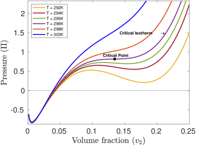
Figure 1: Plot of pressure ($\Pi$) vs. volume fraction ($v_{2}$) at various temperatures. The black dot represents the critical point.

III.2 Pressure and phase diagrams

To characterize the phase transition and the critical phenomenon, we must obtain the relevant phase diagram. The phase diagram is a graphical representation of the variations of pressure, temperature, and volume fraction. The relation among the three quantities is mathematically represented by the equation of state for the osmotic pressure. The osmotic pressure is the thermodynamic force conjugate to the volume fraction $v_{1}$ of the solvent related [4]. The equation of state relating osmotic pressure $\Pi$ with the volume fraction $v_{2}$ and temperature $T$ is given by the following constitutive relation,

$$\Pi=-N_{A}\left(\dfrac{\partial\Psi}{\partial n_{1}}\right)$$ (20)

where $\Psi$ is the total free energy. Using (19) in (20), we obtain the equation of state as,

$$\Pi=-RT\left\{\dfrac{\Theta}{2T}\dfrac{1}{(1+n_{1}\bar{v})^{2}}+\dfrac{1}{1+n_{1}\bar{v}}+\ln{\left(\dfrac{n_{1}\bar{v}}{1+n_{1}\bar{v}}\right)}+\dfrac{S}{(1+n_{1_{0}}\bar{v})^{3}}\left[\left(\dfrac{1+n_{1_{0}}\bar{v}}{1+n_{1}\bar{v}}\right)^{1/3}-\dfrac{1}{2}\left(\dfrac{1+n_{1_{0}}\bar{v}}{1+n_{1}\bar{v}}\right)\right]\right\}$$ (21)

where $N_{A}$ is Avogadro’s number and $R$ is the gas constant. Eq. (21) may also be written in terms of the volume fraction $v_{2}$,

$$\Pi=-RT\left\{\dfrac{\Theta}{2T}(v_{2})^{2}+v_{2}+\ln{\left(1-v_{2}\right)}+S(v_{2_{0}})^{3}\left[\left(\dfrac{v_{2}}{v_{2_{0}}}\right)^{1/3}-\dfrac{1}{2}\left(\dfrac{v_{2}}{v_{2_{0}}}\right)\right]\right\}$$ (22)

Fig. 1 shows the $\Pi-v_{2}$ projection of the phase diagram for a polyacrylamide gel which is obtained using Eq. (22) (the material constants for which are available in [5]): $k_{B}=1.38\times 10^{-23}$ J K^-1, $\Theta=400$ K, $S=600$, $v_{2_{0}}=0.01$, $R=8.3145$ J K^-1 mol^-1. The volume of the individual solvent molecule, $\bar{v}=3.7\times 10^{-28}$ m³, and this value is adopted from [46].

Fig. 1 shows the isotherms at temperatures $T=292\text{ K},294\text{ K},295\text{ K},296\text{ K},298\text{ K and }303\text{ K}$. In Fig. 1, we observe all the salient features typical of a P-V diagram in a discontinuous phase transition. Of all the isotherms, one is the critical isotherm on which lies the critical point, a point of inflection which can be characterized by the critical osmotic pressure $\Pi_{c}$, the critical volume fraction $v_{2_{c}}$ and the critical temperature $T_{c}$. To determine $\Pi_{c}$, $v_{2_{c}}$ and $T_{c}$, we simultaneously solve $\frac{\partial\Pi}{\partial v_{2}}=0$ and $\frac{\partial^{2}\Pi}{\partial v_{2}^{2}}=0$. Due to the equations being strongly nonlinear, they need to be solved numerically. For polyacrylamide gels, we use the values of constants as mentioned earlier and obtain $\Pi_{c},v_{2_{c}}$ and $T_{c}$ as 0.82 Pa, 0.1344 and 296 K respectively, which is shown by the black dot in Fig. 1.

Above the temperature corresponding to the critical isotherm, i.e. for $T>T_{c}$, distinct swollen or shrunken phases do not exist. Hence, no phase transition takes place and a single stable homogeneous ”supercritical gel” phase exists. Below the critical temperature $T<T_{c}$, there is always a certain zone of instability, marked by negative compressibility during which phase transition from a swollen to a shrunken phase takes place. Thus, the critical point serves as the boundary line. Below it, there is a chance of phase transition taking place; but above it, no phase transition occurs.

Resuming our analysis on the stability of different phases, all isotherms below $T_{c}$ contain a zone of negative compressibility. The zone begins with a local maximum and ends with a local minimum. The locus of these extrema is the spinodal curve. It is important to note that negative compressibility is thermodynamically infeasible and is a theoretical artifact that arises from the form of the equation of state. In fact, this is also present in the P-V diagram for van der Waals fluids [5, 47]. Physically no such state of negative compressibility exists. The gel abruptly transitions from a swollen to a shrunken phase at constant pressure. This unphysical outcome might be attributed to the absence of gradient dependent terms in the expression for free energy, thereby accounting for the heterogeneity occurring during phase transition. Experimental evidence [48, 49, 50, 51] indicates that pressure is constant in this region even though it is in non-equilibrium. Nonetheless, the point is that, due to a thermodynamically non-equilibrium nature in this region, the conventional definition of pressure is called into question and requires further research.

III.3 Modified free energy and pressure

The gel in the zone of so-called negative compressibility undergoes spontaneous phase separation by the process of spinodal decomposition [27, 52, 30]. This is inadequately represented in the free energy expression in Eq. (19). To address this limitation, one way would be to use a gradient-enhanced term in the Landau-Ginzburg functional [25, 29, 28, 23, 24]. This functional leads to a generalized chemical potential that drives the diffusion in the system. Specifically, we consider a free energy function that includes a squared gradient term, which should be meaningful under the nonequilibrium conditions underlying phase transition.

Let $\Psi_{grad}$, the free energy term that incorporates gradient dependence, be given by,

$$\Psi_{grad}=\frac{\eta k_{B}T}{2}\left(\dfrac{1+n_{1}\bar{v}}{1+n_{1_{0}}\bar{v}}\right)(\nabla n_{1})^{2}$$ (23)

where, $\eta=\eta_{1}\tilde{T}^{2}+\eta_{2}\tilde{T}+\eta_{3}$ is the scaling parameter of the gradient term. We also have $\eta_{1}=5.8484\times 10^{4}$, $\eta_{2}=-12.3426\times 10^{4}$ and $\eta_{3}=6.4762\times 10^{4}$.

Now, the final form of the free energy ($\Psi_{mod}$) of the system after incorporating the gradient-dependent term is given by,

$$\Psi_{mod}=(1-\kappa)\Psi+\kappa\Psi_{grad}$$ (24)

where $\kappa$ is the gradient energy parameter which plays a crucial role in the region of phase-separation and weighs the contribution of $\Psi$ against $\Psi_{grad}$ [30, 25, 29, 28, 23, 24]. It is evaluated as,

$$\kappa=\{\varphi(1-\varphi_{1})+\varphi_{1}\}\varphi_{2}$$ (25)

where $\varphi=(\gamma_{1}+\gamma_{2})$, $\varphi_{1}=H\left(-\dfrac{\partial^{2}\Psi}{\partial n_{1}^{2}}\right)$, $\varphi_{2}=H\left(-\dfrac{\partial\Psi}{\partial n_{1}}\right)$ with $\gamma_{1}=\tanh{(\omega_{1})}$ and $\gamma_{2}=0.5+0.5\tanh{100(\tanh{\omega_{2}}-0.1)}$. $\gamma_{1}$ and $\gamma_{2}$ are the parameters corresponding to the local maximum and local minimum of the spinodal region respectively. The constituent parameters are given as,

$$\omega_{1}=-2\times 10^{5}[0.5+0.5\tanh{(-\zeta)}]\vartheta\zeta_{1}$$ (26)

$$\omega_{2}=14[0.5+0.5\tanh{(\zeta)}]\vartheta\zeta_{2}$$ (27)

where, $\zeta=\tanh{\left(-\dfrac{1}{(90h)^{2}}\dfrac{\partial^{3}\Psi}{\partial n_{1}^{3}}\right)}$, $\vartheta=\tanh{\left(-\dfrac{1}{(90h)^{0.75}}\dfrac{\partial^{3}\Psi}{\partial n_{1}^{3}}\right)}$, $\zeta_{1}=\exp{\left\{-\dfrac{1}{h^{\phi_{1}}}\left(\dfrac{\partial^{2}\Psi}{\partial n_{1}^{2}}\right)^{2}\right\}}$ and $\zeta_{2}=\exp{\left\{-\dfrac{1}{h^{\phi_{2}}}\left(\dfrac{\partial^{2}\Psi}{\partial n_{1}^{2}}\right)^{2}\right\}}$ with $h^{\phi_{1}}$ and $h^{\phi_{2}}$ being the length scales associated with the local maximum and the local minimum of the spinodal region respectively. Currently adopted expressions for $\phi_{1}$ and $\phi_{2}$ are given by $\phi_{1}=\exp{\left\{-841.6669+838.1726\tilde{T}\right\}}+0.9955(\tilde{T})^{-0.0008}$, $\phi_{2}=\exp{\left\{-427.4063+424.0418\tilde{T}\right\}}+0.9758(\tilde{T})^{-0.0043}$, We also use $h=0.1\times 10^{-14}k_{B}^{4}$ and $\nabla n_{1}=10^{12}$.

Consequently, via Eq. (24), the modified pressure $(\Pi_{mod})$ may be expressed as,

$$\Pi_{mod}=-N_{A}\left(\dfrac{\partial\Psi_{mod}}{\partial n_{1}}\right)$$ (28)

The above modification is consistent with experimental observations [48, 49, 50, 51] and the Maxwell tie-line construction [53] which gives the pressure and the region where the transition from swollen to shrunken phase takes place. In other words, both phases co-exist in this region. In line with [53], a Maxwell tie-line is drawn subtending equal areas between the local maximum and minimum and the tie-line. At any point on the tie-line, both swollen and shrunken phases co-exist in a phase-separated microstructure and the relative volume fraction of each phase may be determined through the lever-arm rule. The locus of intersection of the tie-lines with the isotherms is known as the coexistence curve. Between the coexistence curve and the spinodal curve, the phases are metastable. At lower volume fractions, the metastable phase is predominantly swollen (MSW) and at higher volume fractions, it is predominantly shrunken (MSH). At volume fractions lower than any point on the swollen limb of the coexistence curve, a homogeneously swollen (SW) phase exists, while at volume fractions above the shrunken limb of the coexistence curve, a homogeneously shrunken phase (SH) exists. The coexistence and spinodal curves meet at the critical point.

It is important to characterize the critical point and determine $\Pi_{c}$, $v_{2_{c}}$ and $T_{c}$ so that all three projections of the phase diagram may be represented in terms of reduced dimensionless quantities. One direct advantage of such a representation is that the critical exponents [4] associated with the phase transition may be readily calculated. Another significant advantage is the clear identification of the stable, unstable, and metastable phase boundaries, i.e. the spinodal and coexistence curves.

The phase diagram projection $\Pi$ - $v_{2}$ is redrawn using the reduced pressure $\tilde{\Pi}=\Pi_{mod}/\Pi_{c}$, reduced volume fraction $\tilde{v}_{2}=v_{2}/v_{2_{c}}$ and reduced temperature $\tilde{T}=T/T_{c}$ and shown in Fig. 2. The critical point is more distinctly illustrated in Fig. 2 and so are the stable and unstable zones. For isotherms $\tilde{T}<1$, the part of the isotherm where it is parallel to the horizontal axis, is the region where transition from swollen to shrunken phase takes place. In Fig. 2, the coexistence curve is represented by the black dashed curve while the spinodal curve is represented by the black dash-dotted curve.

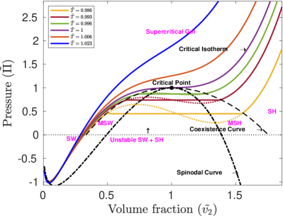
Figure 2: $\tilde{\Pi}$-$\tilde{v_{2}}$ phase diagram denoting the various phases and containing the various isotherms. The black dot denotes the critical point and the black dashed curve represents the coexistence curve. The spinodal curve is represented by the black dash-dotted curve.

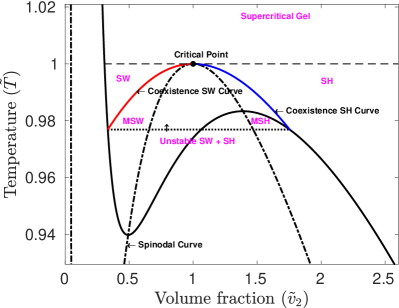
Figure 3: $\tilde{T}-\tilde{v}_{2}$ phase diagram denoting the various phases. The red and blue solid curves represent the swollen and shrunken limbs of the coexistence curve respectively. The black dot denotes the critical point and the black solid curve represents the isobar at $\tilde{\Pi}=0$. The dotted horizontal line at $\tilde{T}=0.976$ corresponds to the phase transition temperature and the black dash-dotted curve represents the spinodal curve.

Fig. 3 shows the $\tilde{T}-\tilde{v_{2}}$ projection of the phase diagram. The solid black curve denotes the isobar $\Pi/\Pi_{c}=0$. Coexistence and spinodal curves may be seen in $\tilde{\Pi}-\tilde{v}_{2}$ projection as well. The swollen limb of the coexistence curve where predominately swollen phase exists is represented by the solid red curve while the shrunken limb of the coexistence curve is represented by the solid blue curve in Fig. 3.

Finally, the $\tilde{\Pi}-\tilde{T}$ projection is shown in Fig. 4. In this figure, the entire coexistence or the phase transition region described in the earlier diagrams (Fig. 2 and Fig. 3) appears as the solid red line. The shrunken and swollen phases outside the phase transition region are also shown in the figure. Also shown is the critical point and the supercritical gel region. The spinodal curve has also been depicted by the black dash-dotted curve in Fig. 3 and Fig. 4.

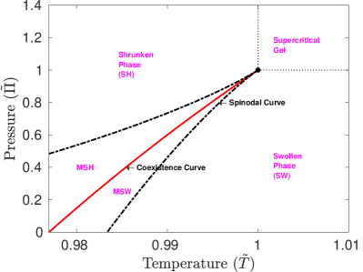
Figure 4: $\tilde{\Pi}-\tilde{T}$ phase diagram denoting the various phases. The red solid curve represents the coexistence curve. The black dash-dotted curve is the spinodal curve. The black dot represents the critical point.

For further analysis of phase transition mechanism, we formulate a method for approaching equilibrium in a system where surface effects, as characterized by a gradient energy given by Eq. (23), play a significant role. In line with the work of [30], the continuity equation corresponding to the free energy of the system as in Eq. (24) may be written as,

$$\dfrac{\partial v_{2}}{\partial t}=\nabla\cdot\{Dv_{2}(1-v_{2})\nabla\mu_{mod}\}$$ (29)

where $D$ is the diffusion coefficient, $v_{2}$ is the volume fraction of polymer which is the order parameter of the system and $\mu_{mod}$ is the chemical potential associated with it. In nonequilibrium systems, the chemical potential $\mu_{mod}$ varies across distinct points, serving as the driving force for the process of diffusion. The chemical potential $\mu_{mod}$ in Eq.(29) is calculated as,

$$\begin{split}\mu_{mod}=&\Psi_{mod}+(1-v_{2})\dfrac{\delta\Psi_{mod}}{\delta v_{2}}\\ =&\Psi_{mod}+(1-v_{2})\left[\dfrac{\partial\Psi_{mod}}{\partial v_{2}}-\nabla\dfrac{\partial\Psi_{mod}}{\partial(\nabla v_{2})}\right]\end{split}$$ (30)

where,

$$\dfrac{\partial\Psi_{mod}}{\partial v_{2}}=\left[(1-\kappa)\dfrac{\partial\Psi}{\partial n_{1}}+\kappa\dfrac{\partial\Psi_{grad}}{\partial n_{1}}+(\Psi_{grad}-\Psi)\dfrac{\partial\kappa}{\partial n_{1}}\right]\dfrac{\partial n_{1}}{\partial v_{2}}$$ (31)

$$\dfrac{\partial\Psi_{mod}}{\partial(\nabla v_{2})}=\kappa\dfrac{\partial\Psi_{grad}}{\partial(\nabla n_{1})}\dfrac{\partial(\nabla n_{1})}{\partial(\nabla v_{2})}$$ (32)

Eq. (29) is analogous to Cahn-Hilliard equation [23] with the difference that the term $Dv_{2}(1-v_{2})$ substitutes for the mobility $M$. Eq. (29) can be used to gain substantial insight into the dynamical aspects of phase change using, say, numerical schemes such as finite difference or Euler’s method, among others.

IV Thermodynamic geometry of gels

The phase diagrams afforded a certain measure of understanding of phase transition in our system. Now, using Ruppeiner’s approach, we attempt to track the evolution of the microstructure throughout this process. Indeed, the nonlinear nature of the manifold on which the microstructural evolution happens should rule out the emergence of unstable regions. Writing Eq. (2) in terms of the fluctuating variables $T$ and $n_{1}$, we obtain the following expression for the squared length of an incremental line element,

$$(\Delta l)^{2}=-\dfrac{1}{k_{B}T}\left(\dfrac{\partial^{2}{\Psi_{mod}}}{\partial{T}^{2}}\right)(\Delta T)^{2}+\dfrac{1}{k_{B}T}\left(\dfrac{\partial^{2}{\Psi_{mod}}}{\partial{n_{1}}^{2}}\right)(\Delta n_{1})^{2}$$ (33)

The (matrix form of the) metric tensor in Eq. (4) is given by

$$\mathbf{g}=\dfrac{1}{k_{B}T}\left[\begin{array}[]{cc}-\dfrac{\partial^{2}{\Psi_{mod}}}{\partial{T}^{2}}&0\\ 0&\dfrac{\partial^{2}{\Psi_{mod}}}{\partial{n_{1}}^{2}}\\ \end{array}\right]$$ (34)

In terms of $T$ and $n_{1}$, the Ricci scalar curvature $R$ may be determined using Eq. (9),

$$R=\dfrac{1}{\sqrt{g}}\left[\dfrac{\partial}{\partial T}\left(\dfrac{1}{\sqrt{g}}\dfrac{\partial g_{22}}{\partial T}\right)+\dfrac{\partial}{\partial n_{1}}\left(\dfrac{1}{\sqrt{g}}\dfrac{\partial g_{11}}{\partial n_{1}}\right)\right]$$ (35)

where $g=-\dfrac{1}{(k_{B}T)^{2}}\dfrac{\partial^{2}{\Psi_{mod}}}{\partial{T}^{2}}\dfrac{\partial^{2}{\Psi_{mod}}}{\partial{n_{1}}^{2}}$ is the determinant of the metric tensor.

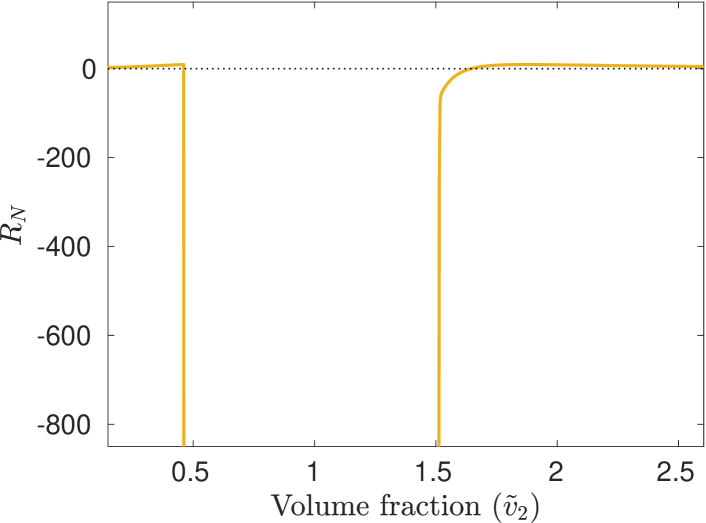
(a)

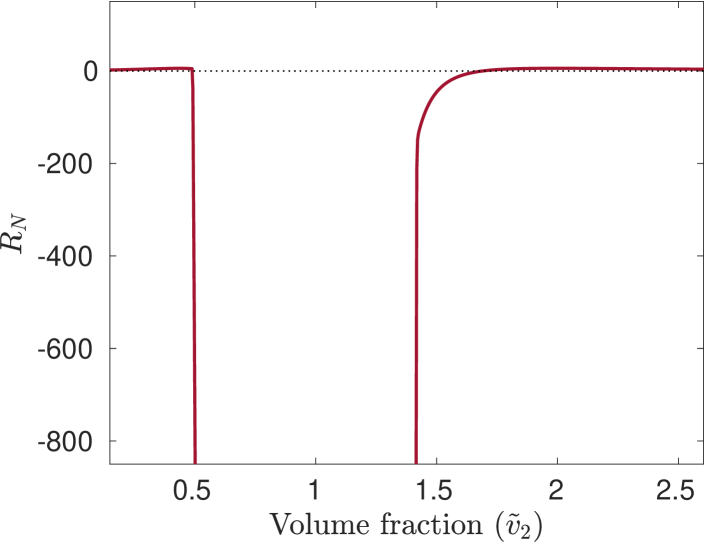
(b)

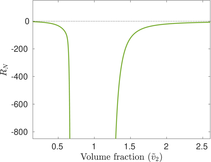
(c)

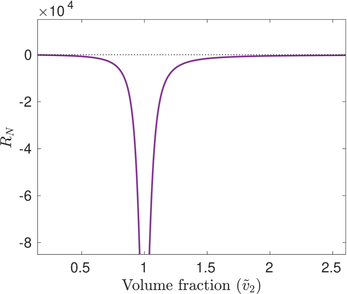
(d)

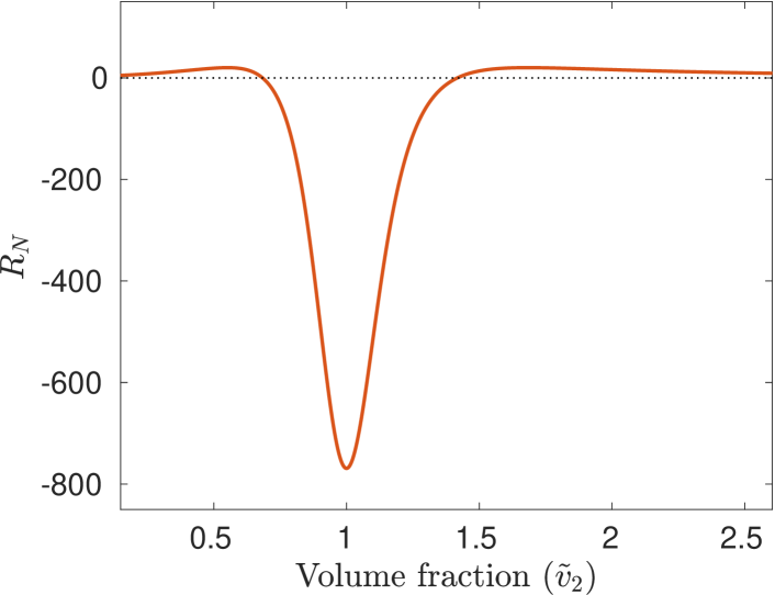
(e)

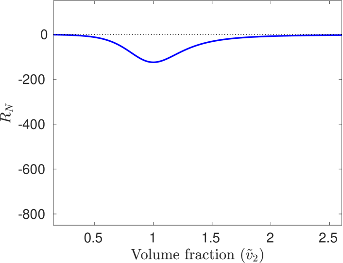
(f)

Figure 5: Plots of normalized scalar curvature $R_{N}$ with volume fraction ($\tilde{v_{2}}$) at temperatures (a) $\tilde{T}=0.986$, (b) $\tilde{T}=0.993$, (c) $\tilde{T}=0.996$, (d) $\tilde{T}=1$, (e) $\tilde{T}=1.006$, (f) $\tilde{T}=1.023$

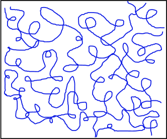
(a) Swollen phase (SW)

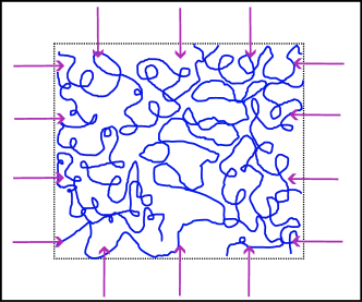
(b) Shrunken phase (SH)

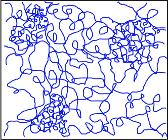
(c) Heterogeneous state with both swollen phase and shrunken phase (Unstable SW + SH)

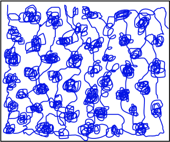
(d) Gel phase at critical point

Figure 6: Schematic representation of the microstructure of different phases of the gel

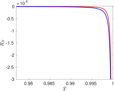
Figure 7: Plot showing the behavior of normalized scalar curvature $R_{N}$ along the swollen limb (top red line) and shrunken limb (bottom blue line) of the coexistence curve.

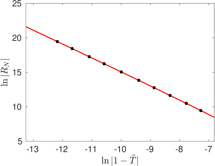
(a)

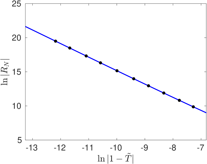
(b)

Figure 8: Plot of $\ln|R_{N}|$ vs $\ln|1-\tilde{T}|$. Black markers denote the numerically obtained data and the solid line denotes the fitted curve. (a) The coexistence swollen phase curve (red line)—the slope is -2.00902. (b) The coexistence shrunken phase curve (blue line)—the slope is -1.99123.

Using the free energy density (Eq. (24)) in Eq. (35), the expression for $R$ is obtained as,

$$R=\dfrac{p}{q}$$ (36)

where,

$$p=-k_{B}\Theta n_{1}\bar{v}s\begin{bmatrix}C_{v}\tilde{T}(1+n_{1_{0}}\bar{v})(r+s)+C_{v}\left\{\tilde{T}s+\tilde{T}\bar{v}n_{1}r+\tilde{T}r+\bar{v}n_{1}s\left(\tilde{T}-\dfrac{\Theta}{T_{c}}\right)\right\}\\ +\tilde{T}\left\{\tilde{T}r+\tilde{T}\bar{v}n_{1}r+\tilde{T}s+\bar{v}n_{1}s\left(\tilde{T}-\dfrac{\Theta}{T_{c}}\right)\right\}\left\{CT_{c}+\dfrac{0.05A(\tilde{T}-1)}{|\tilde{T}-1|^{1.95}}+\dfrac{0.55AD(\tilde{T}-1)}{|\tilde{T}-1|^{1.45}}\right\}\end{bmatrix}$$ (37)

$$q=2C_{v}^{2}\begin{bmatrix}\tilde{T}r+\tilde{T}\bar{v}n_{1}r+\tilde{T}s+\bar{v}n_{1}s\left(\tilde{T}-\dfrac{\Theta}{T_{c}}\right)\end{bmatrix}^{2}$$ (38)

• $r=S\bar{v}n_{1}\left\{-2+3\left(\dfrac{1+n_{1_{0}}\bar{v}}{1+n_{1}\bar{v}}\right)^{2/3}\right\}$,

• $s=6(1+n_{1_{0}}\bar{v})^{2}\left(\dfrac{1+n_{1_{0}}\bar{v}}{1+n_{1}\bar{v}}\right)^{2/3}$.

where $S$ is the constant defined in (14).

We define the normalized scalar curvature $R_{N}=\dfrac{R}{k_{B}}$ in line with [44] and observe its variation with reduced volume $\tilde{v}_{2}$ for reduced temperatures $\tilde{T}=0.986,0.993,0.996,1,1.006$ and $1.023$; the results are shown in Fig. 5. The curvature assumes small to moderate values over a majority of the parametric space except in the vicinity of the spinodal curve and the coexistence region, where it diverges. For $\tilde{T}=1$, divergence of $R_{N}$ is observed only at the critical point $v_{2_{c}}=1$ (see Fig. 5 (d)). For $\tilde{T}>1$, divergence of $R_{N}$ is not observed (see Figs. 5 (e) and (f)).

In the context of black holes, divergence of $R_{N}$ is speculated to have some relation with divergence of the correlation length $\xi$ [44]. We believe that the same holds true for volumetric phase transition and divergence in curvature is directly related to that in the fluctuations of the order parameter $\tilde{v}_{2}$. Thus, density fluctuations are divergent in the coexistence region and at the critical point. Within the coexistence region, density fluctuations manifest as phase segregation at the macroscopic scale, attributed to spinodal decomposition within the spinodal or unstable region and, nucleation and growth in the metastable region. At the critical point, fluctuations cause segregation at the microscopic scale which manifests as critical opalescence in light scattering experiments. Photon correlation spectroscopic studies on polyacrylamide gels [4] have established the existence of a phase segregated microstructure on the coexistence curve which confirms our understanding. In Fig. 6, we have shown some schematic representations of the microstructure in swollen, shrunken, critical and unstable regimes based on our interpretation of curvature and aided by the work in [4]. The gel appears homogeneous in the swollen and shrunken phases and heterogeneous in the unstable and critical regimes. Based on what is known of the Van der Waals fluid system [44], we may expect a homogeneous microstructure in the supercritical regime but with large microscale density fluctuations; see Figs. 5 (e) and (f). But owing to a lack of experimental data pertaining to $C_{v}$ at higher temperatures, further insight at this stage is not available.

Curvature has also been exploited to reveal the nature of interactions among micro-constituents during different stages of phase transition in van der Waals fluids and black holes. For example, the sign of curvature in the case of van der Waals fluid [41] indicates whether the predominant force between fluid molecules is attractive or repulsive for a particular temperature or volume fraction. We examine the variation in the sign of curvature along the coexistence curve on lines similar to [44]. The curvature remains negative for all temperatures leading to the conclusion that no radical change occurs in the nature of interaction with change in volume fraction $v_{2}$ over the entire range of temperatures considered.

Finally, we would like to examine the critical behaviour of $R_{N}$ near the critical point to further establish the universality class of phase transition. We start by examining the critical exponent with which the curvature diverges. To evaluate the exponent, we resort to a numerical technique described in [45]. First we assume a critical-temperature dependent functional form for $R_{N}$ in the vicinity of the critical point and fit the curve to discrete points lying on the swollen and shrunken limbs of the coexistence curve.

$$R_{N}\sim-(1-\tilde{T})^{-\alpha}$$ (39)

or, equivalently,

$$\ln{|R_{N}|}=-\alpha\ln{|1-\tilde{T}|}+\beta$$ (40)

near the critical point. Fig. 8 shows the discrete points and the fitted curves. Along the coexistence swollen phase curve, we get the following fitting result,

$$\ln{|R_{N}|}=-2.00902\ln{|1-\tilde{T}|}-5.01464$$ (41)

The result along the coexistence shrunken phase curve is,

$$\ln{|R_{N}|}=-1.99123\ln{|1-\tilde{T}|}-4.7542$$ (42)

Comparing Eqs. (41) and (42), we can deduce that the slope of $\ln{|R_{N}|}$ vs. $\ln{|1-\tilde{T}|}$ is -2. Thus, the critical exponent associated with scalar curvature is 2. Also, $R_{N}$ as a function of $\tilde{T}$ is given by,

$$R_{N}\sim-(1-\tilde{T})^{-2}$$ (43)

Based on the mean field theory, the critical exponent associated with the correlation length $\xi$ is $0.5$ [3]. So one may define the following relationship between the curvature and the correlation length,

$$R_{N}\sim-\xi^{4}$$ (44)

The critical exponent of 2 and the scaling law of Eq. (44) establish that phase transition in gels indeed belongs to the same universality class as van der Waals fluids and black hole systems [44, 45, 54].

V Conclusion

In view of various practical applications, discontinuous volumetric phase transition in gels is of interest to both scientific and industrial communities. A substantive characterization of phase transition based on an understanding of the microstructure is thus crucial. In the present article, we have studied phase separation dynamics in the light of a Landau-Ginzburg theory in order to gain an understanding of the transformative processes underlying phase transition. We have used Ruppeiner’s thermodynamic approach to probe the microstructure of a polyacrylamide gel undergoing phase transition. The divergence points in the Ricci scalar curvature indicate diverging correlation length and hence large density fluctuations. This implies phase segregation and a heterogeneous microstructure during transition. Further, the uniform negative sign of the curvature indicates no drastic change in the molecular interactions for the range of temperatures considered. Finally, we have numerically calculated the critical exponent associated with the scalar curvature and established a scaling law between curvature and correlation length. We have thus theoretically confirmed that this phase transition belongs to the same universality class as gas-liquid phase transition in van der Waals fluids. We may also draw inferences on the gel microstructure across transitions and across critical points. While the microstructure is phase-segregated during transition and at critical point, no such conclusion can be reached in the supercritical regime with no singularities in curvature post the critical point. In the supercritical regime, from the present approach, we may merely assume that the nature of interactions does not change and that the microstructure is homogeneous, pending a more detailed study where curvature needs to be analyzed at even higher temperatures with more accurate notions of specific heat in line with [55]. In our future work, we would also like to exploit our observations to design efficient supercritical systems for biomedical and structural applications.

References

- Koetting et al. [2015] M. C. Koetting, J. T. Peters, S. D. Steichen, and N. A. Peppas, Stimulus-responsive hydrogels: Theory, modern advances, and applications, Materials Science and Engineering: R: Reports 93, 1 (2015).
- Kamata et al. [2015] H. Kamata, X. Li, U.-i. Chung, and T. Sakai, Design of hydrogels for biomedical applications, Advanced healthcare materials 4, 2360 (2015).
- Shibayama and Tanaka [1993] M. Shibayama and T. Tanaka, Volume phase transition and related phenomena of polymer gels, Responsive gels: volume transitions I , 1 (1993).
- Tanaka et al. [1977] T. Tanaka, S. Ishiwata, and C. Ishimoto, Critical behavior of density fluctuations in gels, Physical Review Letters 38, 771 (1977).
- Tanaka [1978] T. Tanaka, Collapse of gels and the critical endpoint, Physical review letters 40, 820 (1978).
- Dušek and Patterson [1968] K. Dušek and D. Patterson, Transition in swollen polymer networks induced by intramolecular condensation, Journal of Polymer Science Part A-2: Polymer Physics 6, 1209 (1968).
- Amiya and Tanaka [1987] T. Amiya and T. Tanaka, Phase transitions in crosslinked gels of natural polymers, Macromolecules 20, 1162 (1987).
- Katayama and Ohata [1985] S. Katayama and A. Ohata, Phase transition of a cationic gel, Macromolecules 18, 2781 (1985).
- Hirokawa and Tanaka [1984] Y. Hirokawa and T. Tanaka, Volume phase transition in a non-ionic gel, in AIP Conference Proceedings, Vol. 107 (American Institute of Physics, 1984) pp. 203–208.
- Hirotsu et al. [1987] S. Hirotsu, Y. Hirokawa, and T. Tanaka, Volume-phase transitions of ionized n-isopropylacrylamide gels, The Journal of chemical physics 87, 1392 (1987).
- Otake et al. [1988] K. Otake, T. Tsuji, M. Konno, and S. Saito, Preparation of a new hydrogel and porous glass composite membrane, Journal of chemical engineering of Japan 21, 443 (1988).
- Inomata et al. [1990] H. Inomata, S. Goto, and S. Saito, Phase transition of n-substituted acrylamide gels, Macromolecules 23, 4887 (1990).
- Otake et al. [1990] K. Otake, H. Inomata, M. Konno, and S. Saito, Thermal analysis of the volume phase transition with n-isopropylacrylamide gels, Macromolecules 23, 283 (1990).
- Siegel et al. [1988] R. A. Siegel, M. Falamarzian, B. A. Firestone, and B. C. Moxley, ph-controlled release from hydrophobic/polyelectrolyte copolymer hydrogels, Journal of Controlled Release 8, 179 (1988).
- Hirokawa et al. [1984] Y. Hirokawa, T. Tanaka, and S. Katayama, Microbial adhesion and aggregation” ed. kc marshall (1984).
- Ricka and Tanaka [1984] J. Ricka and T. Tanaka, Swelling of ionic gels: quantitative performance of the donnan theory, Macromolecules 17, 2916 (1984).
- Ohmine and Tanaka [1982] I. Ohmine and T. Tanaka, Salt effects on the phase transition of ionic gels, The Journal of Chemical Physics 77, 5725 (1982).
- Siegel and Firestone [1988] R. A. Siegel and B. A. Firestone, ph-dependent equilibrium swelling properties of hydrophobic polyelectrolyte copolymer gels, Macromolecules 21, 3254 (1988).
- Osada [2005] Y. Osada, Conversion of chemical into mechanical energy by synthetic polymers (chemomechanical systems), in Polymer Physics (Springer, 2005) pp. 1–46.
- Tanaka et al. [1982] T. Tanaka, I. Nishio, S.-T. Sun, and S. Ueno-Nishio, Collapse of gels in an electric field, Science 218, 467 (1982).
- Giannetti et al. [1988] G. Giannetti, Y. Hirose, Y. Hirokawa, and T. Tanaka, Molecular electronic devices (1988).
- Flory [1953] P. J. Flory, Principles of polymer chemistry (Cornell university press, 1953).
- Cahn and Hilliard [1958] J. W. Cahn and J. E. Hilliard, Free energy of a nonuniform system. i. interfacial free energy, The Journal of chemical physics 28, 258 (1958).
- Cahn and Hilliard [1959] J. W. Cahn and J. E. Hilliard, Free energy of a nonuniform system. iii. nucleation in a two-component incompressible fluid, The Journal of chemical physics 31, 688 (1959).
- Nauman and Balsara [1989] E. Nauman and N. P. Balsara, Phase equilibria and the landau—ginzburg functional, Fluid Phase Equilibria 45, 229 (1989).
- Binder [1987a] K. Binder, Theory of first-order phase transitions, Reports on progress in physics 50, 783 (1987a).
- Binder [1987b] K. Binder, Dynamics of phase separation and critical phenomena in polymer mixtures, Colloid and Polymer Science 265, 273 (1987b).
- Ariyapadi and Nauman [1990] M. Ariyapadi and E. Nauman, Gradient energy parameters for polymer–polymer–solvent systems and their application to spinodal decomposition in true ternary systems, Journal of Polymer Science Part B: Polymer Physics 28, 2395 (1990).
- He et al. [1996] D. Q. He, S. Kwak, and E. B. Nauman, On phase equilibria, interfacial tension and phase growth in ternary polymer blends, Macromolecular theory and simulations 5, 801 (1996).
- Nauman and He [2001] E. Nauman and D. Q. He, Nonlinear diffusion and phase separation, Chemical Engineering Science 56, 1999 (2001).
- Li and Tanaka [1992] Y. Li and T. Tanaka, Phase transitions of gels, Annual Review of Materials Science 22, 243 (1992).
- Hochberg et al. [1979] A. Hochberg, T. Tanaka, and D. Nicoli, Spinodal line and critical point of an acrylamide gel, Physical Review Letters 43, 217 (1979).
- Hirotsu [1987] S. Hirotsu, Phase transition of a polymer gel in pure and mixed solvent media, Journal of the Physical Society of Japan 56, 233 (1987).
- Tokita and Tanaka [1991] M. Tokita and T. Tanaka, Friction coefficient of polymer networks of gels, The Journal of chemical physics 95, 4613 (1991).
- Li and Tanaka [1989] Y. Li and T. Tanaka, Study of the universality class of the gel network system, The Journal of chemical physics 90, 5161 (1989).
- Ruppeiner [1995] G. Ruppeiner, Riemannian geometry in thermodynamic fluctuation theory, Reviews of Modern Physics 67, 605 (1995).
- Das et al. [2022] S. Das, A. Raza, and D. Roy, Geometric thermodynamics of strain-induced crystallization in polymers, Phys. Rev. E 106, 015005 (2022).
- Ruppeiner [2010] G. Ruppeiner, Thermodynamic curvature measures interactions, American Journal of Physics 78, 1170 (2010).
- Ruppeiner and Bellucci [2015] G. Ruppeiner and S. Bellucci, Thermodynamic curvature for a two-parameter spin model with frustration, Physical Review E 91, 012116 (2015).
- Ruppeiner [2008] G. Ruppeiner, Thermodynamic curvature and phase transitions in kerr-newman black holes, Physical Review D 78, 024016 (2008).
- Ruppeiner and Seftas [2020] G. Ruppeiner and A. Seftas, Thermodynamic curvature of the binary van der waals fluid, Entropy 22, 1208 (2020).
- Ruppeiner et al. [2021] G. Ruppeiner, P. Mausbach, and H.-O. May, Thermodynamic geometry of the gaussian core model fluid, Fluid Phase Equilibria , 113033 (2021).
- Kumara et al. [2022] A. N. Kumara, C. L. A. Rizwan, K. Hegde, M. S. Ali, and K. M. Ajith, Microstructure of five-dimensional neutral gauss–bonnet black hole in anti-de sitter spacetime via criticality, General Relativity and Gravitation 55, 10.1007/s10714-022-03050-y (2022).
- Wei et al. [2019a] S.-W. Wei, Y.-X. Liu, and R. B. Mann, Repulsive interactions and universal properties of charged anti–de sitter black hole microstructures, Phys. Rev. Lett. 123, 071103 (2019a).
- Wei et al. [2019b] S.-W. Wei, Y.-X. Liu, and R. B. Mann, Ruppeiner geometry, phase transitions, and the microstructure of charged ads black holes, Phys. Rev. D 100, 124033 (2019b).
- Das and Roy [2021] S. Das and D. Roy, A poroviscoelasticity model based on effective temperature for water and temperature driven phase transition in hydrogels, International Journal of Mechanical Sciences 196, 106290 (2021).
- Tanaka [1979] T. Tanaka, Phase transitions in gels and a single polymer, Polymer 20, 1404 (1979).
- Pallas and Pethica [1985] N. R. Pallas and B. A. Pethica, Liquid-expanded to liquid-condensed transition in lipid monolayers at the air/water interface, Langmuir 1, 509 (1985), https://doi.org/10.1021/la00064a019 .
- Hifeda and Rayfield [1985] Y. Hifeda and G. Rayfield, Phase transitions in fatty acid monolayers containing a single double bond in the fatty acid tail, Journal of Colloid and Interface Science 104, 209 (1985).
- Hifeda and Rayfield [1992] Y. Hifeda and G. Rayfield, Evidence for first-order phase transitions in lipid and fatty acid monolayers, Langmuir 8, 197 – 200 (1992).
- Crane et al. [1999] J. M. Crane, G. Putz, and S. B. Hall, Persistence of phase coexistence in disaturated phosphatidylcholine monolayers at high surface pressures, Biophysical Journal 77, 3134 (1999).
- Tanaka [1996] H. Tanaka, Coarsening mechanisms of droplet spinodal decomposition in binary fluid mixtures, The Journal of chemical physics 105, 10099 (1996).
- Clerk-Maxwell [1875] J. Clerk-Maxwell, On the dynamical evidence of the molecular constitution of bodies, Nature 11, 357 (1875).
- Kumar and Sarkar [2014] P. Kumar and T. Sarkar, Geometric critical exponents in classical and quantum phase transitions, Phys. Rev. E 90, 042145 (2014).
- Bolmatov et al. [2013] D. Bolmatov, V. Brazhkin, and K. Trachenko, Thermodynamic behaviour of supercritical matter, Nature communications 4, 2331 (2013).