GSDF: 3DGS Meets SDF for Improved Rendering and Reconstruction

Abstract

Presenting a 3D scene from multiview images remains a core and long-standing challenge in computer vision and computer graphics. Two main requirements lie in rendering and reconstruction. Notably, SOTA rendering quality is usually achieved with neural volumetric rendering techniques, which rely on aggregated point/primitive-wise color and neglect the underlying scene geometry. Learning of neural implicit surfaces is sparked from the success of neural rendering. Current works either constrain the distribution of density fields or the shape of primitives, resulting in degraded rendering quality and flaws on the learned scene surfaces. The efficacy of such methods is limited by the inherent constraints of the chosen neural representation, which struggles to capture fine surface details, especially for larger, more intricate scenes. To address these issues, we introduce GSDF, a novel dual-branch architecture that combines the benefits of a flexible and efficient 3D Gaussian Splatting (3DGS) representation with neural Signed Distance Fields (SDF). The core idea is to leverage and enhance the strengths of each branch while alleviating their limitation through mutual guidance and joint supervision. We show on diverse scenes that our design unlocks the potential for more accurate and detailed surface reconstructions, and at the meantime benefits 3DGS rendering with structures that are more aligned with the underlying geometry. Project page: https://city-super.github.io/GSDF.

1 Introduction

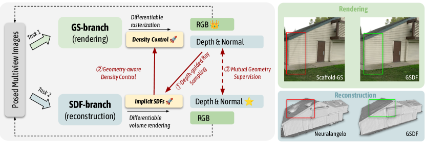
Figure 1: Given posed multi-view images, neural scene representations have achieved extensive advancements for 1) learning high-fidelity rendering [20, 15] and 2) high-quality reconstruction from implicit Signed Distance Fields [29, 17], yet their optimization and rendering processes have normally been seen as a trade-off. Our GSDF proposes a novel dual-branch framework, adopting three ways of mutual guidance (indicated with red lines), achieving enhanced quality for both tasks. We identify the key bottleneck components for each branch (highlighted in yellow blocks), which are generally challenging to optimize or refine on their own, can gain significant benefits from the other side through our design.

Recent advancements in neural scene representations have showcased superior rendering capabilities [20, 21, 15]. However, the lack of explicit geometry arising from their implicit nature makes them hard to support downstream applications, such as robotics [14, 25], physical simulations [33, 7], and XR applications [34, 12], where editing and interaction on concrete scene geometry are often required. Nevertheless, they sparked significant interest in neural surface reconstruction [37, 29, 17, 30, 9], which seek for unified representation that simultaneously models a radiance field and a signed distance field, aligning the density distribution with the distance function with state-of-the-art scene representations as the backbones.

While neural surface reconstruction techniques exhibit superiority in conjunction with neural rendering targets, they often suffer from rendering fidelity decay in comparison to leading methods solely focused on novel view synthesis. Scaling up scenes with complex geometry also remains a challenge, limiting their practical applications. Recent approaches, such as [9, 5] explored using flat Gaussian primitives for surface modeling. While enforcing binary opacity [9] and jointly learned NeuS model [5] to regularize attributes, they also faced degraded rendering quality due to the applied primitive constraints. Despite this, existing work such as Adaptive Shell [32], Binary Occupancy Field [24] and Scaffold-GS [19] have shown that geometry guidance can indeed boost rendering quality with well-regularized spatial structures. Based on these findings, we hypothesize that an optimal blend of both approaches is attainable through a synchronously optimized dual-branch system as shown in Fig. 1. Through extensive experiments, we show that with carefully adapted learning supervisions and optimization strategies, the superiority of both worlds can be preserved via efficient mutual guidances and supervisions, without interfering with the intrinsic properties that contribute to excellence in either neural rendering or reconstruction.

Specifically, our system incorporates a GS-branch for rendering and an SDF-branch for surface reconstruction. Motivated by the strengths of both sides, i.e., fast training for coarse geometry and efficient rasterization from the 3DGS, along with the continuous geometry prior from the neural SDF branch, we propose: 1) Utilizing the rasterized depth from the fast GS-branch to guide ray sampling in the SDF-branch, enhancing the efficiency of volume rendering and avoiding local minima; 2) Employing the SDF-guidance for density control in 3D-GS, guiding the growth of 3D Gaussians in near-surface regions and pruning otherwise. 3) Aligning geometry properties (depth and normal) estimated from both branches. We found this unified system overcomes the limitations of each sides originated from the differences between the rendering methods (i.e., rasterization vs. dense ray sampling), as well as the scene representation (i.e., discrete primitives vs. continuous radiance fields). Furthermore, our framework effortlessly accommodates future advancements for each branch.

Extensive experiments demonstrate that our dual-branch design allows: 1) the GS-branch generates structured primitives closely distributed to the surface, reducing floaters and improving details and edges in view synthesis; 2) an accelerated convergence in the SDF-branch results in superior geometry accuracy and increased surface details.

2 Related work

2.1 Neural Rendering and View Synthesis

Neural Radiance Fields (NeRFs) [20] have achieved remarkable photorealistic rendering quality with view-dependent effects. They adopt Multi-Layer Perceptrons (MLPs) to encode 3D scenes by mapping 3D spatial locations to point-wise color and density, then aggregated into pixel colors through neural volumetric rendering. Because of its volumetric nature and the inductive bias of MLPs, this representation achieves superior performance in novel view synthesis tasks. However, the major challenge is that a large number of points along the ray need to be sampled, thus becoming extremely slow during both training and rendering. The global MLP architecture also limited its modeling capacity, making it hard to be scaled-up to large and complex scenes.

Later research efforts [21, 35, 4, 8] have been made towards more scalable representations. These stream of work largely improves the modeling power of NeRF by shifting the learning burden from the global MLP to locally optimized spatial features. Among them, iNGP [21] achieved SOTA rendering quality with a multi-resolution hash encoding and a lightweight MLP. The proposed hybrid representation has demonstrated impressive capability at capturing very finegrained details in both geometry and appearance.

Setting apart from learning radiance fields via MLP and spatial features, rasterizing geometric primitives, e.g. point clouds, has also been a popular approach for rendering [1, 39]. Despite its efficiency and flexibility, the rendering quality usually suffers from flaws such as discontinuity and outliers. To alleviate such artifacts, attempts have been made such as augmenting points with neural features and incorporating volumetric rendering like NeRF [36]. Nevertheless, these strategies introduces more computes, hence hinder the rendering efficiency. Most recently, 3D Gaussians splatting [15] has revolutionized neural rendering, which employed anisotropic 3D Gaussians as primitives of 3D scenes, which are sorted along depth and splatted onto 2D screen space, then rasterized into pixel colors using $\alpha$-blending. 3D Gaussian Splatting has led to high-quality results with fine-scale details, and is able to be rendered at a real-time frame rate. A follow-up work Scaffold-GS [19] further improves the vanilla 3DGS’s rendering quality and memory efficiency with a hierarchical structure, where anchors are exploited to aligned with the scene geometry and predicts neural Gaussians for more robust rendering. However, these approaches are tailored for view synthesis tasks which does not enforce strict constrained on accurate scene geometry. They tend to learn a volumetric density field that is generally a fuzzy soft shape, from which extracting a high-quality surface is difficult.

2.2 Neural Surface Reconstruction

The success of neural rendering also sparked interest in neural surface reconstruction [22, 37, 29, 17, 30, 38, 38], which generally employed coordinate-based networks to encode scene geometry through occupancy fields or SDF values. The inherent continuity of MLPs coupled with volume rendering yields surfaces that are spatially smooth and complete, often falling short in capturing high-fidelity details and can be slow to optimize. Notably, [17, 32, 24] leveraged multi-resolution hashed feature grids proposed in iNGP [21] to increase the representation power, achieving state-of-the-art reconstructed results. To retain the rendering speed and quality, hybrid approaches have also emerged using a combination of surface and volume rendering [28, 32, 24].

More recently, attempts have been made on learning implicit surface from, or using 3D Gaussian Splatting. For instance, SuGaR [9] encouraged 3D Gaussians to align with the potential surface by approximating them to 2D planar primitives with binary opacity. The concurrent work NeuSG [5] jointly optimized 3D Gaussian Splatting with NeuS [29]. Similar to SuGaR, it also encouraged flat 3D Gaussians whose minimized scaling factor became the normal of 3D Gaussians, that are regularized to be aligned with NeuS predicted normal. NeuS was in turn regularized by the point clouds derived from 3D Gaussians, where the predicted SDF values are enforced to be near zero. Importantly, NeuSG used Vis-MVSNet [40] to obtain dense and coherently structured point clouds that accurately represented the scene’s geometry. However, running MVS can be time-intensive and struggles with processing background regions. Despite the superiority of neural surface reconstruction techniques, a noticeable fidelity gap constantly exists. The regularization imposed on the properties of the Gaussian spheres greatly hindered the rendering quality when compared to original 3DGS.

3 Method

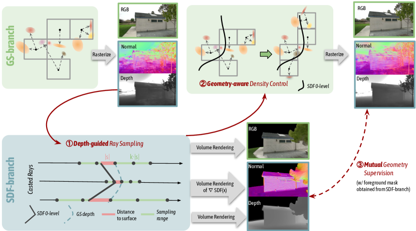
Figure 2: Overview of the proposed method. Our dual-branch framework comprises a GS-branch dedicated to rendering and an SDF-branch focusing on learning neural surfaces. Our design effectively preserves the superiority of rendering with Gaussian primitives [15, 19] in terms of efficiency and fidelity, and also more accurately approximates scene surfaces from an SDF field adapted from NeuS [29]. Concretely, (1) we leverage the efficiency and flexibility advantages of the GS-branch, to render depth maps and guide the ray sampling process of the SDF-branch. For each depth position, we query the SDF-branch to obtain its absolute SDF value $|s|$, and uniformly sample points within $2k|s|$ (e.g. $k=4$). (2) The predicted SDF values from the SDF-branch are in turn used to guide the density control of the GS-branch to grow Gaussian primitives in near-surface regions and prune the ones that are far-away. (3) We further enforce mutual geometry consistency by comparing the depth and normal maps from each branch to encourage more coherent physical alignment between Gaussian primitives and surfaces.

We present a dual-branch framework featuring a GS-branch focusing on efficient and high-quality rendering, and an SDF-branch concentrates on neural implicit surface reconstruction. In Sec. 3.1, we first briefly go through current SOTA rendering techniques including 3D Gaussian Splatting [15] and Scaffold-GS [19]; and representative SDF-based neural implicit surface learning methods including NeuS [29] and Neurolangelo [17]. We show that optimizing solely for either rendering or reconstruction can lead to flaws, for example, floaters in 3DGS, and holes on the learned surface as shown in Fig. 1. We then delve into the details of our proposed dual-branch framework in Sec 3.2. Particularly, we elaborate the use of depth maps rendered from the GS-branch to guide ray sampling of the SDF-branch; and describes our geometry-aware Gaussian density control that results in better structured Gaussian primitives. We further introduce the mutual geometry supervision, which impose an implicit and finer-grained regularization between these two branches. Sec. 3.3 provides more details on our training strategy and loss design.

3.1 Preliminary

3.1.1 3D Gaussian Splatting.

3DGS [15] explicitly represents the scene with 3D Gaussian primitives, cooperating with a tile-based rasterizer to achieve state-of-the-art rendering quality and speed. Each Gaussian primitive is defined by the mean $\mu\in\mathbb{R}^{3}$ and the covariance $\Sigma\in\mathbb{R}^{3\times 3}$:

$$G(x)=e^{-\frac{1}{2}(x-\mu)^{T}\Sigma^{-1}(x-\mu)},$$ (1)

where $x$ is a 3D position within the scene. The tile-based rasterizer is designed to efficiently sort the Gaussians and employ $\alpha$-blending after projecting the 3D Gaussians to the 2D image plane [43]. A gradient-based controller is also proposed to adaptively manage the density of 3D Gaussian. Recently, Scaffold-GS [19] was proposed to make Gaussian primitive more faithful to scene structure and robust to view-dependent effects. Specifically, they used a hierarchical 3D Gaussian scene representation, using anchor points to encode local scene information and spawn local neural Gaussians to render views. Each anchor is optimized with a feature vector that is used to predict the color, center, variance, and opacity of the spawned neural Gaussians.

3.1.2 Neural Implicit SDFs.

NeRF [20] implicitly learns a 3D scene as a continuous volume density and radiance field from multi-view images. Although it can achieve realistic rendering quality, the density-based representation is not designed to accurately present the scene geometry. In contrast, signed distance function (SDF), which can also be regarded as a continuous field, has been widely used to reconstruct scene geometry from 3D point cloud [3, 13, 42, 23]. A stream of work has been dedicated to combining NeRF with SDF to infer neural implicit scene surfaces, representative NeuS [29] introduced SDF to the Neural Radiance Fields by converting the SDF value to the opacity $\alpha_{i}$ with a logistic function:

$$\alpha_{i}=\max\left(\frac{\Phi_{s}\left(f\left(\mathbf{x}_{i}\right)\right)-\Phi_{s}\left(f\left(\mathbf{x}_{i+1}\right)\right)}{\Phi_{s}\left(f\left(\mathbf{x}_{i}\right)\right)},0\right),$$ (2)

where $\Phi_{s}$ denotes a Sigmoid function and $f(x)$ denotes the SDF value of position $x$. Following the classical volume rendering scheme, the predicted color of a ray $r$ is calculated by accumulating weighted colors of the sample points:

$$\mathbf{C}(\mathbf{r})=\sum_{i=1}^{P}T_{i}\alpha_{i}\mathbf{c}_{i},\quad T_{i}=\exp\left(-\sum_{j=1}^{i-1}\alpha_{j}\delta_{j}\right),$$ (3)

where $\delta_{j}$ is the interval between sampled points. Inspired by [21], a multi-resolution hash grid is introduced in [17] to enhance the representation power and accelerate both rendering and training processes. To further prevent the optimization process from falling into local minima, the numerical gradients and a progressive training strategy are also proposed to stabilize the training.

3.2 GSDF: Dual-branch for Rendering and Reconstruction

As shown in Fig. 2, our dual-branch design incorporates a GS-branch and an SDF-branch. We choose Scaffold-GS [19] and NeuS [29] with adapted hash-encoding [10] as backbones for their effectiveness and simplicity. Note that, our framework is not limited to specific methods and can be adapted to accommodate future advanced alternatives.

3.2.1 GS $\to$ SDF: Depth Guided Ray Sampling.

Addressing the computational expenses of the ray-sampling process, techniques like hierarchical sampling [20], occupancy grids [18, 4, 21], early stopping [21], and small proposal networks [2, 24] have been widely adopted, accompanied with CUDA accelerations. When input depth maps are available, either from ground truth sensor collections or monocular estimation, samples can be strategically placed around surface regions. For effective optimization of the Signed Distance Field (SDF), proximity to the structure of interest during point sampling is crucial.

Unlike conventional methods relying on its own predicted SDF values [29, 17, 26] to guide ray sampling, we employ the GS-branch as the structure proximity, circumventing the chicken-and-egg dilemma. Inspired from [35] where the more efficient branch is used to provide coarse geometry guidance for follow-up optimizations, we leverage the rendered depth maps from the GS-branch to narrow down the ray sampling range of the SDF-branch. Despite Gaussian primitives are less precise in modeling scene geometry, they excel in efficiency and flexibility, offering the SDF-branch sufficient geometric clues without much time overhead.

Consider a ray emitted from a camera center $\vec{o}$ pointing towards direction $\vec{v}$, the corresponding depth value $D$ rendered from the GS-branch is given by:

$$D=\sum_{i\in N}d_{i}\sigma_{i}\prod_{j=1}^{i-1}(1-\sigma_{j}),$$ (4)

where $N$ represents the number of 3D Gaussians encountered by the ray, $\sigma_{i}$ is the opacity of each Gaussian primitive, and $d_{i}$ the distance between the $i$-th 3D Gaussian and the camera center. When optimizing the SDF-branch, points are sampled around $\vec{o}+D\cdot\vec{v}$. Importantly, rather than employing a constant range across all rays, we adapt the sampling range based on the predicted SDF values $s$ at varying depths:

$$s=\mathcal{F}_{sdf}(\vec{o}+D\cdot\vec{v}),$$ (5)

where $\mathcal{F}_{sdf}$ is a two-layer MLP of the SDF-branch, used for predicting the SDF value at a given spatial position. The sampling range is defined as: $r=[\vec{o}+(D-k|s|)\cdot\vec{v},o+(D+k|s|)\cdot\vec{v}]$. Inspired by NeRF’s [20] hierarchical sampling strategy, we define a coarse and a fine sampling range with $k=3$ and $k=1$ respectively, as illustrated in Fig. 2. We then uniformly sample $M$ points along the ray within each range .

3.2.2 SDF $\to$ GS: Geometry-aware Gaussian Density Control.

Prior methods have tried to learn scene surfaces from 3DGS by making 3D Gaussians flat with nearly binary opacity, basically treating 3D Gaussians as surface primitives, similar to mesh triangles without the water-tight restriction. Results showed that such constraints can lead to degraded rendering quality and incomplete surfaces. In contrast, we do not encourage the flattening of 3D Gaussian primitives, but instead improve the distribution of Gaussian primitives via a geometry-aware density control strategy. On top of the original gradient-based density control criteria, we additionally leverage the zero-level set of the SDF-branch to identify whether a Gaussian primitive is close to or deviates from the surface. We query the SDF-branch with the position of Gaussian primitives. Primitives with smaller absolute SDF values are deemed to be closer to the surface, and vice versa.

Growing operator.

For each Gaussian primitive located at position $c$, we obtain its SDF value $s=\mathcal{F}_{sdf}(c)$ from the SDF-branch. The criteria for Gaussian growth then becomes:

$$\epsilon_{g}=\nabla_{g}+\omega_{g}\mu(s),$$ (6)

where $\nabla_{g}$ is the averaged gradient of Gaussian primitives accumulated across $K$ training iteration, as in Scaffold-GS [19]; $\mu(s)=\exp\left(-s^{2}/(2\sigma^{2})\right)$ is a Gaussian function that converts the predicted SDF value to a positive effecting factor, whose value monotonically decreases with the distance deviated from the zero level. The parameter $\omega_{g}$ controls the significance of geometric guidance. Once $\epsilon_{g}>\tau_{g}$, new Gaussian primitives will be added if none exists.

Pruning operator.

Similarly, on top of the original opacity-based pruning criteria, we additionally prune Gaussian primitives that are far away from the surface, i.e. with large SDF values. Mathematically, the prune criteria is:

$$\epsilon_{p}=\sigma_{a}-\omega_{p}(1-\mu(s)),$$ (7)

where $\sigma_{a}$ is the aggregated opacity values of Gaussian primitives over $K$ training iterations, representing the transparency level of each Gaussian. We balance transparency and SDF contribution with the weight $\omega_{p}$ in the equation. Anchors with $\epsilon_{p}<\tau_{p}$ will be pruned.

3.2.3 GS $\leftrightarrow$ SDF: Mutual Geometry Supervision.

To enhance both rendering and reconstruction outcomes, our framework incorporates a mutual supervision between two branches, leveraging depth and normal as pivotal geometric features to facilitate this interconnection. Specifically, for the SDF-branch, per-view depth map $D_{sdf}$ is rendered via the volumetric rendering principle, and normal map $N_{sdf}$ is inferred by volumetric rendering of the SDF gradients. As for the GS-branch, we compute per-view depth map $D_{gs}$ following Eq. 4, and regard the direction of the smallest scaling factor to be the normal of each 3D Gaussian, similar to [9, 5, 6]. To render the normal map for each camera view, we accumulate the normal of the 3D Gaussians using $\alpha$-blending: $N_{gs}=\sum_{i\in N}n_{i}\sigma_{i}\prod_{j=1}^{i-1}(1-\sigma_{j})$, where $n_{i}$ is the estimated normal of the $i$-th 3D Gaussian.

3.3 Training Strategy and Loss Design

The GS-branch is supervised by rendering losses $\mathcal{L}_{1}$ and $\mathcal{L}_{\text{SSIM}}$ between the rendered RGB images and ground truth. The volume regularization term $\mathcal{L}_{vol}$ is added following [19]. The full loss function of the GS-branch is defined as:

$$\mathcal{L}_{\text{gs}}=\lambda_{1}\mathcal{L}_{1}+(1-\lambda_{1})\mathcal{L}_{\text{SSIM}}+\lambda_{vol}\mathcal{L}_{vol},$$ (8)

where $\lambda_{1}$ and $\lambda_{vol}$ are weighting coefficients.

The SDF-branch is supervised by the $\mathcal{L}_{1}$ rendering loss with Eikonal penalties and curvature discrepancies:

$$\mathcal{L}_{\text{sdf}}=\mathcal{L}_{1}+\lambda_{\text{eik}}\mathcal{L}_{\text{eik}}+\lambda_{\text{curv}}\mathcal{L}_{\text{curv}},$$ (9)

where $\mathcal{L}_{\text{eik}}$ addresses the Eikonal loss, ensuring gradients of the predicted SDF field are normalized; $\mathcal{L}_{\text{curv}}$ denotes the curvature loss, which promotes surface smoothness following common practices [17, 26]. The coefficients $\lambda_{\text{eik}}$ and $\lambda_{\text{curv}}$ balance the influence of loss terms.

The mutual geometry supervision comprises the depth and normal consistency losses applied on both branches , formulated as:

$$\mathcal{L}_{mutual} =\lambda_{d}\mathcal{L}_{d}+\lambda_{n}\mathcal{L}_{n}$$ (10)

$$=\lambda_{d}\|D_{gs}-D_{sdf}\|+\lambda_{n}(1-\frac{|N_{gs}\cdot N_{sdf}|}{\|N_{gs}\|\times\|N_{sdf}\|}),$$

where $\mathcal{L}_{d}$ and $\mathcal{L}_{n}$ are depth and normal discrepancies between two branches; $\lambda_{n}$ and $\lambda_{n}$ balance their importance.

Finally, the total loss for the joint learning is defined as:

$$\mathcal{L}=\mathcal{L}_{\text{gs}}+\mathcal{L}_{\text{sdf}}+\mathcal{L}_{mutual}.$$ (11)

The hyper-parameter settings are detailed in the supplementary material.

4 Experiment

4.1 Experimental Setup

Datasets.

We conducted comprehensive evaluations on rendering and reconstruction quality using $11$ real-world scenes from publicly available datasets: $7$ available scenes from Mip-NeRF360 [2], $2$ scenes from DeepBlending [11] and $2$ scenes in Tanks$\&$Temples [16], covering a variety of indoor and outdoor scenarios. The camera poses and initial point clouds are provided by COLMAP [27].

Implementation and Baselines.

We implemented our dual-branch model based on 1) Scaffold-GS [19] and 2) NeuS [29] enhanced with its hash-grid variant [10] following practice of [17]. The hash grid resolution spans from $2^{5}$ to $2^{11}$ with $16$ levels. Each hash entry has a feature dimension of $4$ and the maximum number of hash entries of each level is $2^{21}$. $8$ hash resolutions were activated at the beginning of the optimization, and a finer level was added every $2,000$ iteration. We set off by firstly training the GS-branch for $15k$ iterations, then jointly training both branches for $30k$ iterations. To stabilize the optimization, we allow Gaussian primitives to be grown and pruned in the first $30k$ iterations, and warm-up the SDF-branch for $5k$ iterations without depth-guided ray sampling. Note that our system is not limited to specific rendering and reconstruction backbones, and instead can be adapted to work with other existing or future models.

We evaluated our method against SOTA rendering and reconstruction approaches respectively. In terms of rendering, we compared with Scaffold-GS [19], 3D-GS [15] and Mip-NeRF360 [2], and report PSNR, SSIM [31], and LPIPS [41] on test datasets for quantitative comparisons. We trained the 3D-GS [15] and Scaffold-GS [19] with $45$k to align with our configurations. For reconstruction, we compared with Neuralangelo [17] due to its state-of-the-art reconstruction quality, instant-NSR [10] implemented as our SDF-branch, and SuGaR [9] as a fair baseline which reconstructs geometry from 3D Gaussian primitives.

4.2 Results Analysis

Table 1: Rendering Comparisons against baselines over three benchmark scenes. 3D-GS [15], Scaffold-GS [19], and GSDF initialized the Gaussian primitives with points given by COLMAP [27], while Scaffold-GS (rand) and GSDF (rand) randomly initialized the Gaussian primitives.

Dataset	Mip-NeRF360			Tanks&Temples			Deep Blending
Method Metrics	PSNR $\uparrow$	SSIM $\uparrow$	LPIPS $\downarrow$	PSNR $\uparrow$	SSIM $\uparrow$	LPIPS $\downarrow$	PSNR $\uparrow$	SSIM $\uparrow$	LPIPS $\downarrow$
3D-GS [15]	28.89	0.857	0.209	26.73	0.858	0.210	29.44	0.899	0.248
Mip-NeRF360 [2]	29.23	0.844	0.207	26.82	0.854	0.199	29.40	0.901	0.245
Scaffold-GS [19]	29.34	0.863	0.200	27.29	0.869	0.182	30.37	0.908	0.238
GSDF	29.38	0.865	0.185	27.37	0.875	0.156	30.38	0.909	0.223
Scaffold-GS (rand)	27.84	0.817	0.259	26.37	0.838	0.230	29.12	0.895	0.260
GSDF (rand)	28.05	0.830	0.229	26.55	0.852	0.197	29.57	0.899	0.244

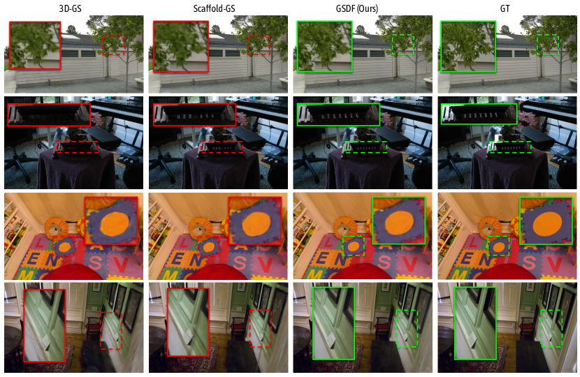
Figure 3: Qualitative comparisons of GSDF against GS-based baselines [15, 19] across diverse datasets [16, 2, 11]. As shown from the above highlighted patches, our method constantly outperformed baselines, especially in modeling delicate geometries (1st & 2nd row), texture-less and less observations regions (3rd & 4th row) that are quite common in larger scenes.

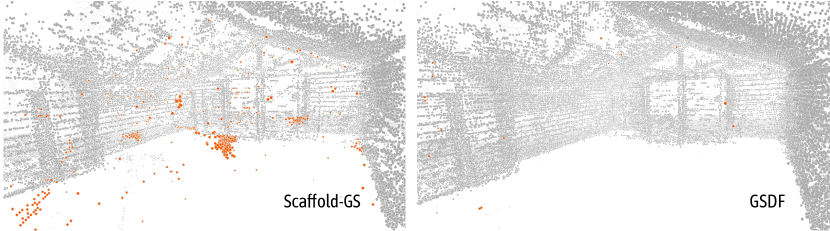
Figure 4: Anchor distributions. We visualized Gaussian primitives from Scaffold-GS and GSDF. Orange points identify floaters deviated from the potential surfaces. Our method yielded more surface-aligned primitives with regularized structure. This is critical for synthesizing clean novel views (less floater artifacts), reducing redundant primitives and supporting downstream tasks that demand accurate geometries.

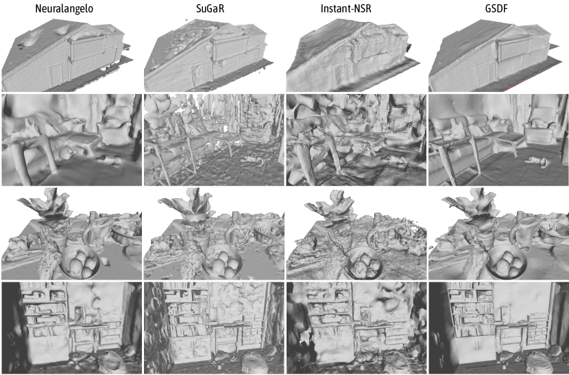
Figure 5: Reconstruction Comparison. We visualized the reconstructed meshes from Neuralangelo [17], SuGaR [9], Instant-NSR [10] (our SDF-branch), and Ours. Our results exhibited more accurate structures and better geometry.

Rendering Comparisons.

Our GSDF retained high rendering quality compared to the SOTA 3D-GS based methods. The quantitative metrics against 3D-GS [15], Mip-NeRF360 [2], and Scaffold-GS [19] are reported in Tab. 1. For all three datasets, GSDF consistently outperformed state-of-the-art methods, showcasing significant improvements in all metrics. Notably, the prominent improvements in LPIPS metric indicated that our method effectively captured high-frequency scene details, and rendered perceptually better results than baselines.

Notably, our method excelled in achieving high rendering quality in texture-less areas, as showcased in Fig. 3. Such behaviour aligned with our design motivation for geometry-aware density control, which effectively pruned the floating Gaussian primitives and grew more near the potential surface as shown in Fig. 4.

Specifically, in texture-less areas where the vanilla 3D Gaussians struggled to pass the growing threshold due to small accumulated gradients, our method adeptly overcame this limitation by also taking SDF values into consideration. Our geometry-aware density control also effectively eliminated floaters and reduced redundant primitives, yielding better structured primitives and hence improved the robustness of novel view rendering, as illustrated in Fig. 1 and 3. Additionally, we also experimented with randomly initializes Gaussian primitives on Scaffold-GS and our method. Quantitative results are presented in Tab. 1, showcasing the advantages of our geometric guidance. Further visual results can be found in the supplementary material. During inference, novel view rendering is performed via the GS-branch only. Hence our rendering speed remained the same as SOTA approaches [15, 19].

Reconstruction Comparisons.

In the absence of ground truth mesh for quantitative evaluation in real-world captures, we followed [9] and qualitatively assessed the mesh quality converted from the neural SDF. As illustrated in Fig. 5, our method reconstructed more complete and detailed meshes compared to baseline methods. Our method was effective in bypassing local minima, preventing the generation of holes in the meshes, as shown in Fig. 5. It can be noticed that Neuralangelo [17] struggled in complex and intricate cases, such as indoor scenes; whereas ours exhibited robust reconstruction results across diverse scenes, which can be attributed to the effectiveness of depth guidance from the GS-branch and the mutual geometric supervision. On the other hand, meshes extracted from SuGaR [9] appeared to be non-manifold with broken topological relationships; in contrast, our extracted mesh was smooth and continuous, where high-frequency details were also well preserved. It is also noteworthy that the optimization of SDF field in previous methods were often time-consuming because of the exhaustive, self-guided ray sampling. For example, Neuralangelo [17] required about $12$-hour optimization with $2$ GPUs to produce results in Fig. 5, whereas ours were significantly more efficient, achieving comparable and even better results within a $2$-hour training on a single GPU. For additional experiments conducted under the same number of training iterations, refer to the supplementary material.

4.3 Ablation Studies

Table 2: Quantitative Results on Ablation Studies. We separately listed the rendering metrics for each ablation described in Sec. 4.3.

Dataset	Mip-NeRF360			Tanks&Temples			Deep Blending
Method Metrics	PSNR $\uparrow$	SSIM $\uparrow$	LPIPS $\downarrow$	PSNR $\uparrow$	SSIM $\uparrow$	LPIPS $\downarrow$	PSNR $\uparrow$	SSIM $\uparrow$	LPIPS $\downarrow$
GSDF (Full)	29.38	0.865	0.185	27.37	0.875	0.156	30.38	0.909	0.223
w/o geometric supervision	29.27	0.862	0.196	27.18	0.865	0.191	30.21	0.907	0.234
w/o depth-guided sampling	29.26	0.863	0.196	27.30	0.873	0.159	30.17	0.908	0.228
w/o geometry-aware densification	29.29	0.863	0.196	27.29	0.870	0.179	30.25	0.908	0.236

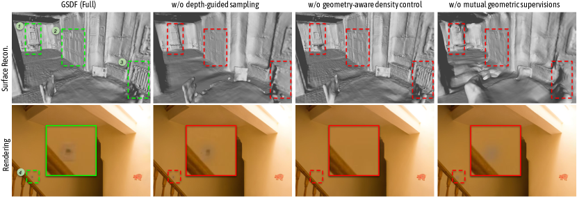
Figure 6: Ablation studies. Visualizations of the reconstructed meshes and rendered images from 1) our full method, 2) ours w/o depth-guided ray sampling, 3) ours w/o geometry-aware density control, and 4) ours w/o geometric supervision. We highlight the degradation of quality using numbered patches.

In this section, we conducted detailed examinations of each individual module to verify the effectiveness of each design. Quantitative metrics and qualitative visualizations can be found in Tab. 2 and Fig. 6.

Depth-Guided Ray Sampling.

To evaluate the effectiveness of our depth-guided ray sampling, as detailed in Sec 3.2, we conducted an ablation using the original stratified ray sampling approach [20]. Results show that the ablated setting led to overly smoothed surfaces, failing to present finer geometry patterns such as the heater and doors, as depicted in the $2$nd column in Fig. 6 (patch 2 & 3). The less accurate SDF also affected rendering to some extent, where the sticker on the wall became more blurred compared to our full model result.

Geometry-aware Gaussian Density Control.

We replaced the proposed geometry-aware Gaussian density control with the pruning and growing strategy utilized in Scaffold-GS [19] to evaluate its efficacy. From the rendering example in the 3rd column in Fig. 6, we can see that the sticker was missed by Gaussian primitives (patch 4), probably due to the small accumulated gradients on the large texture-less wall. From the reconstruction result, we can also notice the absence of thin objects such as table legs and the chandelier (patch 1).

Mutual Geometric Supervision.

We ablated the proposed mutual geometric supervision by setting both $\lambda_{d}$ and $\lambda_{n}$ to $0$ (Eq. 10). A drastic decay in surface quality can be observed whilst some details were omitted in rendering. This finding indicated that neural rendering is much more tolerant than neural surface reconstruction. Without explicitly aligning the structure of Gaussian primitives with SDF-derived geometry during the optimization, these two branches can diverge and both end up in sub-optimal status.

5 Limitation

Like many SDF-based reconstruction methods, the training speed is not as efficient as primitive-based methods using fast rasterization approaches. Consequently, the inclusion of the SDF-branch reduces the training speed of the GS-branch, which could be a drawback when immediate model training is essential. Moreover, SDF struggles with reconstructing transparent and semi-transparent objects, limiting the effectiveness of geometry guidance in these regions.

6 Conclusion

In this work, we introduced a dual-branch framework that leverages the strengths of both 3D-GS and SDF, showcasing its potential to achieve enhanced rendering and reconstruction quality while maintaining efficiency in both training and inference. The inherent differences in two implicit representations, rendering approaches, and supervision loss pose a challenge to the seamless integration of the two. We therefore consider a bidirectional mutual guidance approach to circumvent these restrictions. Three types of guidance have been introduced and validated in our framework, namely: 1) depth guided sampling (GS$\rightarrow$SDF), 2) geometry-aware Gaussian density control (SDF$\rightarrow$GS); and 3) mutual geometry supervision (GS$\leftrightarrow$SDF). Our extensive results demonstrate the efficiency and joint performance improvement on both tasks. As the two branches maintain their original architectures, we keep their efficiency during inference, allowing room for potential enhancements by substituting each branch with more advanced models in the future. We envision our model to benefit applications demanding high-quality rendering and geometry, including embodied environments, physical simulation, and immersive VR experiences.

7 Supplementary Material

The following sections are organized as follows: 1) The first section elaborates on the implementation details of GSDF, covering hyper-parameters and curvature loss. 2) We then show additional experimental results. 3) Lastly, we delve into limitations and future directions.

7.1 Implementation details

7.1.1 Configurations.

Below, we enumerate the hyper-parameters used in our experiments:

• The variance $\sigma^{2}$ for the Gaussian function in Eq. 6 and 7 is set to 0.005.

• For the rendering loss discussed in Sec. 3.3, we set $\lambda_{1}=0.2$ and $\lambda_{vol}=0.01$, in consistency with the configurations specified in Scaffold-GS [19].

• For the SDF-branch, we set $\lambda_{eik}=0.1$ and implement an adaptive scheme for $\lambda_{curv}$. Specifically, $\lambda_{curv}$ increases linearly from $0$ to $1$ over the first $2000$ iterations, after which it remains at $0.05$ for subsequent iterations. This strategy is based on our observation that increasing the weight of the curvature loss significantly encourages the convergence of the SDF to a geometric outline.

• For the mutual geometry loss, we assign $\lambda_{d}=0.5$ and $\lambda_{n}=0.01$.

7.1.2 Curvature Loss.

While Neuralangelo [17] derives the curvature loss from a discrete Laplacian, we follow a more robust and explicit method as described in PermutoSDF [26]. For any given point, we randomly perturb it within the tangent plane orthogonal to its normal. The curvature loss is then measured by the cosine similarity of normals between the original point and its perturbed counterpart.

7.2 More experiments

7.2.1 Reconstruction with $500$k iterations.

As discussed in Sec. 4, optimizing the SDF is a time-intensive process. While our GS-branch assists in the convergence of the SDF-branch, we conjecture that further improvements could be made through additional iterations. Hence, we train our method for $500$k iterations, which is consistent with Neuralangelo [17]. Additionally, we show results of Neuralangelo trained using our configurations ($30$k iterations) for fair comparison. As shown in Fig.7, our method achieves superior reconstruction quality compared to Neuralangelo[17] and Instant-NSR [10] (our SDF-branch) with the same training iterations.

7.2.2 Rendering comparison with random initialization.

In Sec. 3.2, we discussed how the SDF-branch can improve the rendering quality of the GS-branch. This enhancement is particularly noticeable when Gaussian primitives are randomly initialized, as shown in Fig. 8 and Fig. 9.

7.2.3 Per-scene Results.

We list the per-scene quality metrics (PSNR, SSIM, and LPIPS) used in our rendering evaluation in Sec. 4 for all considered methods, as shown from Tab. 3 to Tab. 8.

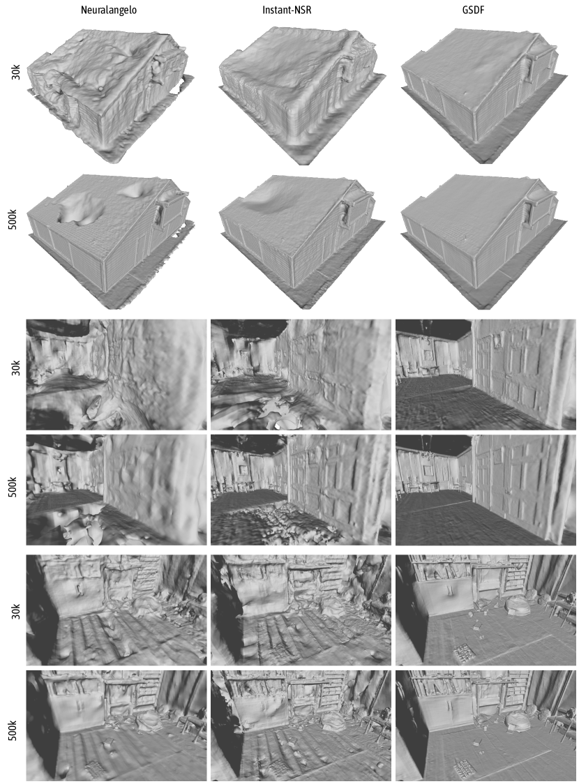
Figure 7: Reconstruction comparison with $30$k and $500$k training iterations.

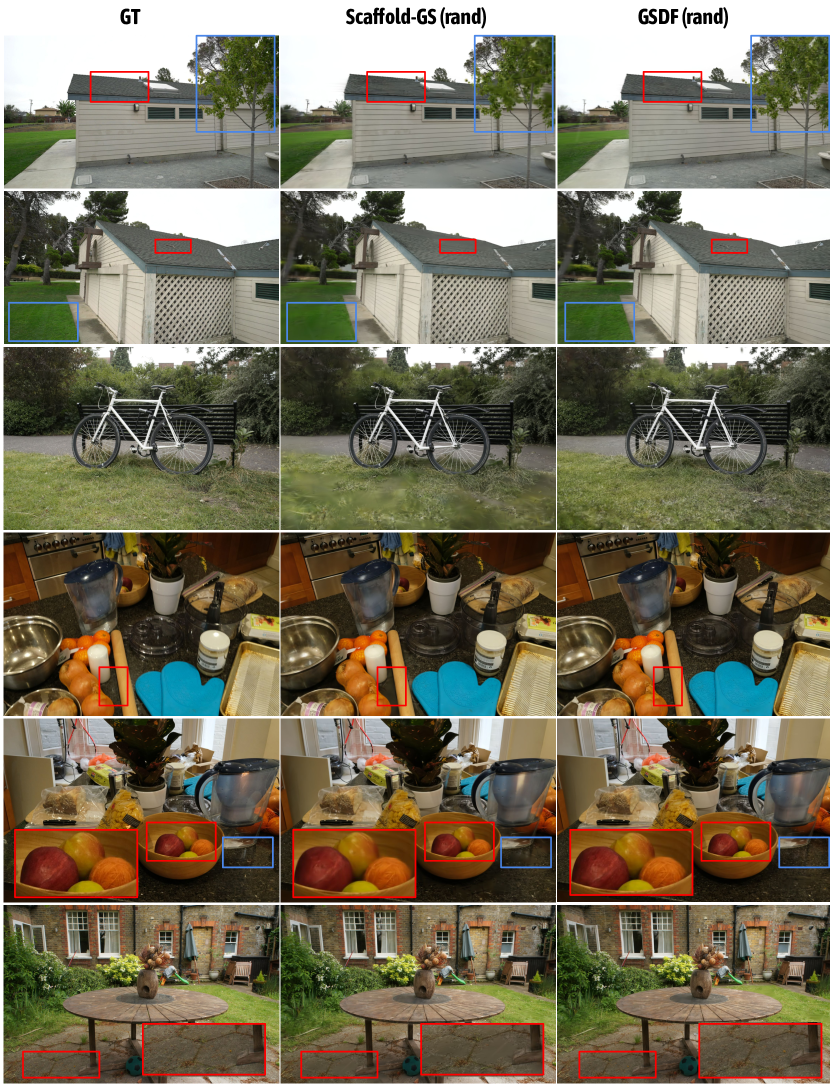
Figure 8: Rendering Comparison (Part 1). We compare rendering results between Scaffold-GS [19] and our method. Despite Gaussian primitives being randomly initialized, posing a challenge where 3D-GS based methods can easily overfit training views. The highlighted patches indicate that our method is superior in expressing finer details in both geometry and appearance.

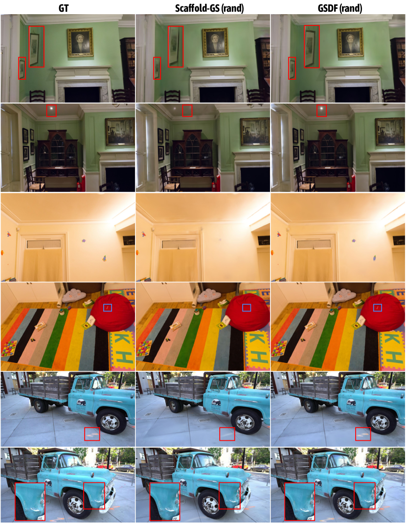
Figure 9: Rendering Comparison (Part 2) - Cont.

Table 3: SSIM scores for Mip-NeRF360 [2] scenes.

Methods Scenes	bicycle	garden	stump	room	counter	kitchen	bonsai
3D-GS [15]	0.707	0.819	0.758	0.925	0.914	0.933	0.945
Mip-NeRF360 [2]	0.685	0.813	0.744	0.913	0.894	0.920	0.941
Scaffold-GS [19]	0.721	0.814	0.765	0.933	0.920	0.934	0.951
Scaffold-GS (rand)	0.633	0.776	0.652	0.920	0.898	0.914	0.928
GSDF	0.724	0.824	0.757	0.937	0.923	0.936	0.954
GSDF (rand)	0.682	0.800	0.625	0.929	0.909	0.929	0.936

Table 4: PSNR scores for Mip-NeRF360 [2] scenes.

Methods Scenes	bicycle	garden	stump	room	counter	kitchen	bonsai
3D-GS [15]	24.46	26.63	26.31	31.68	29.25	31.69	32.19
Mip-NeRF360 [2]	24.37	26.98	26.40	31.63	29.55	32.23	33.46
Scaffold-GS [19]	24.63	26.59	26.58	32.44	29.93	31.99	33.24
Scaffold-GS (rand)	23.48	26.09	22.88	31.84	29.00	30.50	31.08
GSDF	24.61	26.91	26.06	32.46	30.11	31.93	33.60
GSDF (rand)	24.09	26.25	21.92	32.01	29.17	31.45	31.43

Table 5: LPIPS scores for Mip-NeRF360 [2] scenes. rand denotes randomly initialized Gaussian primitives.

Method Scenes	bicycle	garden	stump	room	counter	kitchen	bonsai
3D-GS [15]	0.313	0.175	0.309	0.194	0.180	0.113	0.176
Mip-NeRF360 [2]	0.301	0.170	0.261	0.211	0.204	0.127	0.176
Scaffold-GS [19]	0.289	0.182	0.302	0.178	0.173	0.112	0.165
Scaffold-GS (rand)	0.397	0.239	0.428	0.205	0.206	0.144	0.196
GSDF	0.261	0.158	0.290	0.165	0.159	0.106	0.155
GSDF (rand)	0.328	0.196	0.416	0.181	0.183	0.118	0.182

Table 6: SSIM scores for Tanks&Temples [16] and Deep Blending [11] scenes. rand denotes randomly initialized Gaussian primitives.

Methods Scenes	Truck	Barn	Dr Johnson	Playroom
3D-GS [15]	0.861	0.855	0.908	0.900
Mip-NeRF360 [2]	0.857	0.851	0.901	0.900
Scaffold-GS [19]	0.869	0.869	0.908	0.908
Scaffold-GS (rand)	0.845	0.832	0.892	0.898
GSDF	0.873	0.877	0.909	0.909
GSDF (rand)	0.853	0.851	0.898	0.900

Table 7: PSNR scores for Tanks&Temples [16] and Deep Blending [11] scenes. rand denotes randomly initialized Gaussian primitives.

Methods Scenes	Truck	Barn	Dr Johnson	Playroom
3D-GS [16]	25.24	28.21	29.04	29.84
Mip-NeRF360 [2]	24.91	28.74	29.14	29.66
Scaffold-GS [19]	25.80	28.77	29.86	30.89
Scaffold-GS (rand)	24.93	27.82	28.58	29.66
GSDF	25.81	28.93	29.87	30.89
GSDF (rand)	24.99	28.11	29.09	30.04

Table 8: LPIPS scores for Tanks&Temples [16] and Deep Blending [11] scenes. rand denotes randomly initialized Gaussian primitives.

Methods Scenes	Truck	Barn	Dr Johnson	Playroom
3D-GS [15]	0.197	0.223	0.248	0.248
Mip-NeRF360 [2]	0.159	0.239	0.237	0.252
Scaffold-GS [19]	0.172	0.192	0.236	0.239
Scaffold-GS (rand)	0.217	0.243	0.262	0.258
GSDF	0.1351	0.176	0.225	0.222
GSDF (rand)	0.184	0.210	0.247	0.241

7.3 Limitations and Future Works

Currently, our method is not tailored to handle challenging scenes with reflections and intense lighting variations, such as those found in indoor environments. However, we have observed that employing more structured and surface-aligned Gaussian primitives holds promise in capturing such view-dependent appearance changes with improved scene geometry. Furthermore, the performance of our SDF-branch significantly lags behind the GS-branch, leading to extended training durations compared to Scaffold-GS [19] only. Hence, improving the efficiency of the MLP-based SDF-branch is a crucial direction for future research.

References

- [1] Aliev, K.A., Sevastopolsky, A., Kolos, M., Ulyanov, D., Lempitsky, V.: Neural point-based graphics. In: Computer Vision–ECCV 2020: 16th European Conference, Glasgow, UK, August 23–28, 2020, Proceedings, Part XXII 16. pp. 696–712. Springer (2020)
- [2] Barron, J.T., Mildenhall, B., Verbin, D., Srinivasan, P.P., Hedman, P.: Mip-nerf 360: Unbounded anti-aliased neural radiance fields. In: Proceedings of the IEEE/CVF Conference on Computer Vision and Pattern Recognition. pp. 5470–5479 (2022)
- [3] Boulch, A., Marlet, R.: Poco: Point convolution for surface reconstruction. In: Proceedings of the IEEE/CVF Conference on Computer Vision and Pattern Recognition (CVPR). pp. 6302–6314 (June 2022)
- [4] Chen, A., Xu, Z., Geiger, A., Yu, J., Su, H.: TensoRF: Tensorial radiance fields. In: ECCV (2022). https://doi.org/10.1007/978-3-031-19824-3_20
- [5] Chen, H., Li, C., Lee, G.H.: Neusg: Neural implicit surface reconstruction with 3d gaussian splatting guidance. arXiv preprint arXiv:2312.00846 (2023)
- [6] Cheng, K., Long, X., Yang, K., Yao, Y., Yin, W., Ma, Y., Wang, W., Chen, X.: Gaussianpro: 3d gaussian splatting with progressive propagation. arXiv preprint arXiv: (2024)
- [7] Feng, Y., Feng, X., Shang, Y., Jiang, Y., Yu, C., Zong, Z., Shao, T., Wu, H., Zhou, K., Jiang, C., et al.: Gaussian splashing: Dynamic fluid synthesis with gaussian splatting. arXiv preprint arXiv:2401.15318 (2024)
- [8] Fridovich-Keil, S., Yu, A., Tancik, M., Chen, Q., Recht, B., Kanazawa, A.: Plenoxels: Radiance fields without neural networks. In: Proceedings of the IEEE/CVF Conference on Computer Vision and Pattern Recognition. pp. 5501–5510 (2022)
- [9] Guédon, A., Lepetit, V.: Sugar: Surface-aligned gaussian splatting for efficient 3d mesh reconstruction and high-quality mesh rendering. arXiv preprint arXiv:2311.12775 (2023)
- [10] Guo, Y.C.: Instant neural surface reconstruction (2022), https://github.com/bennyguo/instant-nsr-pl
- [11] Hedman, P., Philip, J., Price, T., Frahm, J.M., Drettakis, G., Brostow, G.: Deep blending for free-viewpoint image-based rendering 37(6), 257:1–257:15 (2018)
- [12] Jiang, Y., Yu, C., Xie, T., Li, X., Feng, Y., Wang, H., Li, M., Lau, H., Gao, F., Yang, Y., et al.: Vr-gs: A physical dynamics-aware interactive gaussian splatting system in virtual reality. arXiv preprint arXiv:2401.16663 (2024)
- [13] Kazhdan, M., Bolitho, M., Hoppe, H.: Poisson surface reconstruction. In: Proceedings of the fourth Eurographics symposium on Geometry processing. vol. 7, p. 0 (2006)
- [14] Keetha, N., Karhade, J., Jatavallabhula, K.M., Yang, G., Scherer, S., Ramanan, D., Luiten, J.: Splatam: Splat, track & map 3d gaussians for dense rgb-d slam. arXiv preprint arXiv:2312.02126 (2023)
- [15] Kerbl, B., Kopanas, G., Leimkühler, T., Drettakis, G.: 3d gaussian splatting for real-time radiance field rendering. ACM Transactions on Graphics 42(4) (2023)
- [16] Knapitsch, A., Park, J., Zhou, Q.Y., Koltun, V.: Tanks and temples: Benchmarking large-scale scene reconstruction. ACM Transactions on Graphics 36(4) (2017)
- [17] Li, Z., Müller, T., Evans, A., Taylor, R.H., Unberath, M., Liu, M.Y., Lin, C.H.: Neuralangelo: High-fidelity neural surface reconstruction. In: Proceedings of the IEEE/CVF Conference on Computer Vision and Pattern Recognition. pp. 8456–8465 (2023)
- [18] Liu, L., Gu, J., Zaw Lin, K., Chua, T.S., Theobalt, C.: Neural sparse voxel fields. Advances in Neural Information Processing Systems 33, 15651–15663 (2020)
- [19] Lu, T., Yu, M., Xu, L., Xiangli, Y., Wang, L., Lin, D., Dai, B.: Scaffold-gs: Structured 3d gaussians for view-adaptive rendering (2023)
- [20] Mildenhall, B., Srinivasan, P.P., Tancik, M., Barron, J.T., Ramamoorthi, R., Ng, R.: Nerf: Representing scenes as neural radiance fields for view synthesis. In: ECCV (2020)
- [21] Müller, T., Evans, A., Schied, C., Keller, A.: Instant neural graphics primitives with a multiresolution hash encoding. ACM Transactions on Graphics (ToG) 41(4), 1–15 (2022)
- [22] Oechsle, M., Peng, S., Geiger, A.: Unisurf: Unifying neural implicit surfaces and radiance fields for multi-view reconstruction. In: Proceedings of the IEEE/CVF International Conference on Computer Vision. pp. 5589–5599 (2021)
- [23] Park, J.J., Florence, P., Straub, J., Newcombe, R., Lovegrove, S.: Deepsdf: Learning continuous signed distance functions for shape representation. In: The IEEE Conference on Computer Vision and Pattern Recognition (CVPR) (June 2019)
- [24] Reiser, C., Garbin, S., Srinivasan, P.P., Verbin, D., Szeliski, R., Mildenhall, B., Barron, J.T., Hedman, P., Geiger, A.: Binary opacity grids: Capturing fine geometric detail for mesh-based view synthesis. arXiv preprint arXiv:2402.12377 (2024)
- [25] Rosinol, A., Leonard, J.J., Carlone, L.: Nerf-slam: Real-time dense monocular slam with neural radiance fields. In: 2023 IEEE/RSJ International Conference on Intelligent Robots and Systems (IROS). pp. 3437–3444. IEEE (2023)
- [26] Rosu, R.A., Behnke, S.: Permutosdf: Fast multi-view reconstruction with implicit surfaces using permutohedral lattices. In: Proceedings of the IEEE/CVF Conference on Computer Vision and Pattern Recognition. pp. 8466–8475 (2023)
- [27] Schonberger, J.L., Frahm, J.M.: Structure-from-motion revisited. In: Proceedings of the IEEE conference on computer vision and pattern recognition. pp. 4104–4113 (2016)
- [28] Turki, H., Agrawal, V., Bulò, S.R., Porzi, L., Kontschieder, P., Ramanan, D., Zollhöfer, M., Richardt, C.: Hybridnerf: Efficient neural rendering via adaptive volumetric surfaces. arXiv preprint arXiv:2312.03160 (2023)
- [29] Wang, P., Liu, L., Liu, Y., Theobalt, C., Komura, T., Wang, W.: Neus: Learning neural implicit surfaces by volume rendering for multi-view reconstruction. arXiv preprint arXiv:2106.10689 (2021)
- [30] Wang, Y., Han, Q., Habermann, M., Daniilidis, K., Theobalt, C., Liu, L.: Neus2: Fast learning of neural implicit surfaces for multi-view reconstruction. 2023 IEEE/CVF International Conference on Computer Vision (ICCV) pp. 3272–3283 (2022), https://api.semanticscholar.org/CorpusID:254564276
- [31] Wang, Z., Bovik, A., Sheikh, H., Simoncelli, E.: Image quality assessment: from error visibility to structural similarity. IEEE Transactions on Image Processing 13(4), 600–612 (2004). https://doi.org/10.1109/TIP.2003.819861
- [32] Wang, Z., Shen, T., Nimier-David, M., Sharp, N., Gao, J., Keller, A., Fidler, S., Müller, T., Gojcic, Z.: Adaptive shells for efficient neural radiance field rendering. arXiv preprint arXiv:2311.10091 (2023)
- [33] Xie, T., Zong, Z., Qiu, Y., Li, X., Feng, Y., Yang, Y., Jiang, C.: Physgaussian: Physics-integrated 3d gaussians for generative dynamics. arXiv preprint arXiv:2311.12198 (2023)
- [34] Xu, L., Agrawal, V., Laney, W., Garcia, T., Bansal, A., Kim, C., Rota Bulò, S., Porzi, L., Kontschieder, P., Božič, A., et al.: Vr-nerf: High-fidelity virtualized walkable spaces. In: SIGGRAPH Asia 2023 Conference Papers. pp. 1–12 (2023)
- [35] Xu, L., Xiangli, Y., Peng, S., Pan, X., Zhao, N., Theobalt, C., Dai, B., Lin, D.: Grid-guided neural radiance fields for large urban scenes. In: CVPR (2023). https://doi.org/10.1109/CVPR52729.2023.00802
- [36] Xu, Q., Xu, Z., Philip, J., Bi, S., Shu, Z., Sunkavalli, K., Neumann, U.: Point-nerf: Point-based neural radiance fields. In: Proceedings of the IEEE/CVF Conference on Computer Vision and Pattern Recognition. pp. 5438–5448 (2022)
- [37] Yariv, L., Gu, J., Kasten, Y., Lipman, Y.: Volume rendering of neural implicit surfaces. Advances in Neural Information Processing Systems 34, 4805–4815 (2021)
- [38] Yariv, L., Hedman, P., Reiser, C., Verbin, D., Srinivasan, P.P., Szeliski, R., Barron, J.T., Mildenhall, B.: Bakedsdf: Meshing neural sdfs for real-time view synthesis. arXiv preprint arXiv:2302.14859 (2023)
- [39] Yifan, W., Serena, F., Wu, S., Öztireli, C., Sorkine-Hornung, O.: Differentiable surface splatting for point-based geometry processing. ACM Transactions on Graphics (TOG) 38(6), 1–14 (2019)
- [40] Zhang, J., Yao, Y., Li, S., Luo, Z., Fang, T.: Visibility-aware multi-view stereo network. arXiv preprint arXiv:2008.07928 (2020)
- [41] Zhang, R., Isola, P., Efros, A.A., Shechtman, E., Wang, O.: The unreasonable effectiveness of deep features as a perceptual metric. In: Proceedings of the IEEE Conference on Computer Vision and Pattern Recognition (CVPR) (June 2018)
- [42] Zhao, T., Alliez, P., Boubekeur, T., Busé, L., Thiery, J.M.: Progressive discrete domains for implicit surface reconstruction. In: Computer Graphics Forum. vol. 40, pp. 143–156. Wiley Online Library (2021)
- [43] Zwicker, M., Pfister, H., Van Baar, J., Gross, M.: Ewa volume splatting. In: Proceedings Visualization, 2001. VIS’01. pp. 29–538. IEEE (2001)