Spherically symmetric configurations in the quadratic $f(R)$ gravity

Abstract

We study spherically symmetric configurations of the quadratic $f(R)$ gravity in the Einstein frame. We found the global qualitative behavior of the metric and the scalaron field for all static solutions satisfying the conditions of asymptotic flatness. These solutions are proved to be regular everywhere except for a naked singularity at the center; they are uniquely determined by the total mass $\mathfrak{M}$ and the “scalar charge” $Q$ characterizing the strength of the scalaron field at spatial infinity. The case $Q=0$ yields the Schwarzschild solution, but an arbitrarily small $Q\neq 0$ leads to the appearance of a central naked singularity having a significant effect on the neighboring region, even though the space-time metric in the outer region is practically insensitive to the scalaron field. Approximation procedures are developed to derive asymptotic relations near the naked singularity and at spatial infinity, and the leading terms of the solutions are presented. We investigate the linear stability of the static solutions with respect to radial perturbations and numerically estimate the range of parameters corresponding to stable/unstable configurations.

Keywords: modified gravity, $f(R)$ gravity, scalar fields, naked singularities

I Introduction

Modification of General Relativity (GR) by a Lagrangian in the form of a nonlinear function $f(R)$ of the scalar curvature $R$ is, perhaps, the simplest one and has long been the subject of numerous studies and applications (see [1, 2, 3] for reviews). Compared to GR, such $f(R)$ gravity theory contains one extra scalar degree of freedom, which can be used for modelling a wide variety of phenomena, from the early inflationary regime [4, 5, 6], consistent with current observations [7], to dark energy and dark matter at later epoch [8, 9, 10, 11, 12, 13, 14, 15, 16, 17, 18].

Natural questions arise about the possible effects of modified gravity in models of isolated systems that can simulate real astrophysical objects. In particular, spherically symmetric (SS) configurations in modified gravity theories have attracted considerable attention in view of various aspects related to the black-hole no-hair theorems, stability properties, global space-time structure etc (see, e.g., [19, 20, 21, 22, 23, 24, 25, 26] and references therein).

In the present paper, we investigate asymptotically flat SS systems and their stability in the framework of the quadratic $f(R)$ gravity. We study these issues using the transition to the convenient Einstein frame. This enables us to use a number of results on minimally coupled scalar fields in General Relativity dealing with the properties of SS systems, “no-hair theorems,” naked singularities etc (see, e.g., [27, 28, 29, 30, 31, 32]). Systems with naked singularities (NS), if they really exist in nature, could be extremely interesting. Indeed, in the modern cosmological epoch, the effects of the modified gravity are expected to be very weak in astrophysical objects, but they can manifest themselves in the extreme conditions near classical NS. On the other hand, there is a widespread opinion that systems with NS do not exist in the universe according to the Penrose’s Cosmic Censorship hypothesis [33, 34]. This hypothesis has never been proven, and its discussion shifts to issues of stability and fine-tuning of the input data [35, 36, 37, 38, 39]. Apparently, the existence and stability of NS depends on the types of configurations involved and, perhaps, on the specific parameter regions in concrete models [40, 41, 42, 43].

Static SS solutions in $f(R)$ gravity were studied earlier in [21], where the existence of NS at the center was pointed out. However, the consideration of [21] is incomplete: it is essentially based on numerical computations, and some of its assumptions may be questioned or at least require rigorous justification. First of all, one must be sure that regular solutions with all possible configuration parameters satisfying the assumption of asymptotic flatness do exist for all positive values of the radial variable $r$. This is a non-trivial question in case of a nonlinear system; indeed, there are examples of static spherically symmetric configurations where “spherical” singularities arise at finite values of $r>0$ [30, 44]. Another crucial point is how to restrict the parameters of the asymptotic expansion near NS in the case of asymptotically flat solutions. It is important to note that correct asymptotics near NS is essential for the investigation of stability by means of linear perturbations.

Our paper is organized as follows. In Section II, we review the general relations of $f(R)$ gravity as regards the transition to the Einstein frame. Section III concentrates on the quadratic $f(R)$ model. Field equations in the Einstein frame are written in Section IV for the case of a non-stationary SS metric. In Section V, we prove that all SS solutions with nonzero scalar field satisfying the asymptotic-flatness conditions exist for all $r>0$ and may have singularity only at $r=0$. Also in this Section, asymptotic formulas near NS are obtained which are further used in numerical calculations. In Section VI we write down equations for perturbations. In Section VII we use numerical calculations to illustrate the static solutions and to study their linear stability. In Section VIII, we discuss our results. The details concerning the proof of the existence and uniqueness and justification of approximation methods are given in appendices.

II Basic equations and notation

In $f(R)$ gravity, the standard Lagrangian of General Relativity in the gravitational action is replaced by a more general function of the scalar curvature $R$:

$$S_{g}=-\frac{1}{2\kappa}\int d^{4}x\,\sqrt{-g}\,f(R)\,,$$

where $\kappa=8\pi G$, and $G$ is Newton’s gravitational constant. The corresponding dynamical equations for the physical metric $g_{\mu\nu}$ (Jordan frame) are [1, 2, 3]

$$f^{\prime}(R)R_{\mu\nu}-\frac{1}{2}g_{\mu\nu}f(R)+\left(\square-\nabla_{\mu}\nabla_{\nu}\right)f^{\prime}(R)=\kappa T_{\mu\nu}\,,$$ (1)

where $T_{\mu\nu}=T_{\nu\mu}$ is the energy-momentum tensor of non-gravitational fields satisfying the covariant conservation law

$$\nabla_{\nu}T^{\mu\nu}=0\,.$$ (2)

There is a well-known procedure [1, 2] to represent the equations of the $f(R)$ gravity, written for the physical metric $g_{\mu\nu}$ (Jordan frame), in the form of the usual Einstein equations for a conformally transformed metric $\hat{g}_{\mu\nu}$ (Einstein frame)

$$g_{\mu\nu}=e^{-2\xi}\hat{g}_{\mu\nu}\,,\quad e^{2\xi}=f^{\prime}(R)\,,$$ (3)

accompanied by equations for an additional canonically normalized scalar field (SF) $\phi=\sqrt{6/\kappa}\,\xi$. In this paper, we will describe this scalar field (the scalaron) by the dimensionless scalar $\xi$.

The self-interaction potential $W(\xi)$ of the scalar field $\xi$ can be introduced parametrically as follows:

$$e^{2\xi}=f^{\prime}(u)\,,\quad W(\xi)=\frac{1}{2}e^{-4\xi}\left[f(u)-f^{\prime}(u)u\right]\,.$$ (4)

The extrema of this potential are located at the values of $\xi$ corresponding to the values of $u$ satisfying the equation $uf^{\prime}(u)=2f(u)$. The quadratic part of the potential around its absolute minimum determines the scalaron mass $\mu$ :

$$\mu^{2}=\frac{1}{3}\left[\frac{1}{f^{\prime\prime}(u)}-\frac{u}{f^{\prime}(u)}\right]\,,$$

where the right-hand side is evaluated at the minimum of the potential. Non-observation [45, 46] of the scalaron-induced Yukawa forces [47] between non-relativistic masses leads to a lower bound on the scalaron mass (see also [10, 11, 48]):

$$\mu\geq 2.7~{}\text{meV}\quad\text{at 95\% C.L.}$$ (5)

This lower bound leads to a rather small corresponding length scale $l_{\mu}=1/\mu$.

Denote,

$$\quad\hat{T}_{\mu\nu}=e^{-2\xi}T_{\mu\nu}\,.$$ (6)

To avoid confusion due to the presence of two metrics, we emphasize that, from this point on, “hats” correspond to the Einstein frame [1, 2], in which covariant differentiation, raising and lowering indexes are performed with the metric tensor $\hat{g}_{\mu\nu}$. On the account of (3) and (4), equation (1) leads to the following equations in the Einstein frame:

$$\hat{R}_{\mu\nu}-\frac{1}{2}\hat{g}_{\mu\nu}\hat{R}=\hat{T}^{(\xi)}_{\mu\nu}+\kappa\hat{T}_{\mu\nu}\,,$$ (7)

where

$$\hat{T}^{(\xi)}_{\mu\nu}=6\partial_{\mu}\xi\,\partial_{\nu}\xi-\hat{g}_{\mu\nu}\left[3\xi_{,\alpha}\xi_{,\beta}\hat{g}^{\alpha\beta}-W(\xi)\right]\,.$$ (8)

Equations (7) are supplemented by the equation for the scalaron $\xi$:

$$\hat{\nabla}_{\alpha}\hat{\nabla}^{\alpha}\xi=-\frac{1}{6}\frac{\partial W}{\partial\xi}+\frac{1}{6}\kappa\hat{T}\,,\quad\hat{T}=\hat{g}^{\mu\nu}\hat{T}_{\mu\nu}\,.$$ (9)

The system of equations (7), (9) is equivalent to the fourth-order equations (1).

The covariant conservation law (2) also must be rewritten in the Einstein frame. For the energy-momentum tensor, we have

$$\hat{\nabla}_{\mu}\hat{T}^{\mu}{}_{\nu}=-\hat{T}\partial_{\nu}\xi\,,\quad\hat{T}=\hat{g}_{\alpha\beta}\hat{T}^{\alpha\beta}\,.$$ (10)

The equation of motion of a test body in the Einstein frame can be obtained directly from the variational principle leading to

$$\frac{\hat{\delta}\hat{u}^{\mu}}{d\hat{s}}=-\left(\hat{g}^{\mu\nu}-\hat{u}^{\mu}\hat{u}^{\nu}\right)\partial_{\mu}\xi\,,$$ (11)

where $\hat{u}^{\mu}=dx^{\mu}/d\hat{s}$, $d\hat{s}=\sqrt{\hat{g}_{\alpha\beta}dx^{\alpha}dx^{\beta}}$, and $\hat{\delta}$ stands for the covariant derivative in the Einstein frame along the particle trajectory.

III Quadratic $f(R)$ gravity

In what follows, we deal with the simplest model, in which

$$f(R)=R-\frac{R^{2}}{6\mu^{2}}\,,$$ (12)

where $\mu$ is the scalaron mass. In the original inflationary model due to Starobinsky [4], described by this Lagrangian, the scalaron mass has relatively large value $\mu\approx 3\cdot 10^{13}$ GeV [7]. However, in this paper we focus mainly on mathematical properties of the model and allow for arbitrary values of $\mu$.

The scalaron potential (4) for model (12) is

$$W(\xi)=\frac{3}{4}\mu^{2}\left(1-e^{-2\xi}\right)^{2}\,.$$ (13)

It is monotonically increasing with $\xi$ in the domain $\xi\geq 0$ asymptotically rising to a plateau. In the case of an asymptotically flat space-time in the initial (Jordan) frame, we assume that the scalar curvature vanishes at spatial infinity; correspondingly, $\xi=\frac{1}{2}\ln[f^{\prime}(R)]\to 0$.

For most of astrophysical systems with continuous distributions of matter, we expect $\xi$ to be very small. For $|\xi|\ll 1$, we have

$$W(\xi)\approx 3\mu^{2}\xi^{2}\,.$$ (14)

In a static case, we deal with metric $g_{\mu\nu}\equiv g_{\mu\nu}({\boldsymbol{r}})$; $g_{0i}\equiv 0$, yielding

$$\hat{\Delta}\xi\equiv-\frac{1}{\sqrt{-\hat{g}}}\frac{\partial}{\partial x^{i}}\left[\sqrt{-\hat{g}}\hat{g}^{ij}\frac{\partial\xi}{\partial x^{i}}\right]=\mu^{2}\xi-\frac{\kappa}{6}\hat{T}\,,$$ (15)

where $i,j=1,2,3$.

As noted above, the value of the scalaron mass $\mu$ is bounded from below by (5) so as not to contradict the existing observations. A somewhat stronger lower bound, $\mu\gtrsim 4.4$ meV, arises in the consideration of the scalaron as a dark-matter candidate [17, 18]. Such a mass corresponds to the length scale $l_{\mu}=\mu^{-1}\lesssim 4.5\cdot 10^{-3}$ cm, which is a very small value in the astrophysical realm. In the case of an astrophysical object with mass $\mathfrak{M}$ and gravitational radius $r_{g}=2G\mathfrak{M}$, we typically deal with a very large dimensionless quantity $\mu r_{g}\gg 1$. This allows us to make a general estimate for the value of $\xi$ inside a sufficiently smooth distribution of $\hat{T}$. Indeed, equation (15) can be written in a form that may be considered as a source of asymptotic approximations:

$$\xi=\frac{\kappa}{6\mu^{2}}\hat{T}-\frac{1}{\mu^{2}}\hat{\Delta}\xi\,,$$ (16)

with the last term on the right-hand side regarded as a small perturbation. This gives us a simple approximate formula

$$\xi\approx\frac{\kappa}{6\mu^{2}}\left(\hat{T}-\frac{1}{\mu^{2}}\hat{\Delta}\hat{T}\right)\,.$$ (17)

This formula is applicable if $\mu^{2}\hat{T}\gg\hat{\Delta}\hat{T}$, which, however, may fail to be satisfied at the boundary of the body, where (17) must be replaced by a more exact relation.

IV Spherically symmetric configurations

IV.1 Field equations in the Einstein frame

The metric of a spherically symmetric space-time in the Schwarzschild (curvature) coordinates can be written as

$$d\hat{s}^{2}=e^{\alpha}dt^{2}-e^{\beta}dr^{2}-r^{2}\left(d\theta^{2}+\sin^{2}\theta d\varphi^{2}\right),$$ (18)

where $r>0$, $\alpha\equiv\alpha(t,r)$, $\beta\equiv\beta(t,r)$. The nontrivial Einstein equations (7) in this case are

$$\frac{\partial}{\partial r}\left[r\left(e^{-\beta}-1\right)\right]=-\kappa r^{2}\hat{T}_{0}^{0}$$

$$\quad-r^{2}\left[3e^{-\alpha}\left(\frac{\partial\xi}{\partial t}\right)^{2}+3e^{-\beta}\left(\frac{\partial\xi}{\partial r}\right)^{2}+W(\xi)\right]\,,$$ (19)

$${re^{-\beta}\frac{\partial\alpha}{\partial r}+e^{-\beta}-1}=-\kappa r^{2}\hat{T}_{1}^{1}$$

$$\quad+r^{2}\left[3e^{-\alpha}\left(\frac{\partial\xi}{\partial t}\right)^{2}+3e^{-\beta}\left(\frac{\partial\xi}{\partial r}\right)^{2}-W(\xi)\right]\,,$$ (20)

$$\frac{\partial\beta}{\partial t}=\kappa\hat{T}_{0}^{1}+6r\frac{\partial\xi}{\partial t}\frac{\partial\xi}{\partial r}\,,$$ (21)

where $\xi\equiv\xi(t,r)$, and the structure of $\hat{T}_{\mu\nu}$ corresponds to the spherically symmetric case.

Equation (9) yields

$$e^{-\frac{\alpha+\beta}{2}}\left[\frac{\partial}{\partial t}\left(e^{\frac{\beta-\alpha}{2}}\frac{\partial\xi}{\partial t}\right)-\frac{1}{r^{2}}\frac{\partial}{\partial r}\left(r^{2}e^{\frac{\alpha-\beta}{2}}\frac{\partial\xi}{\partial r}\right)\right]\,$$

$$=-\frac{1}{6}\left[W^{\prime}(\xi)-{\kappa}\hat{T}\right]\,.$$ (22)

Note that, for $\xi\equiv 0$ and $\hat{T}=0$, we get the Schwarzschild solution.

IV.2 Static SS solutions

In the case of a static isolated regular configuration, the quantities $\alpha$, $\beta$ and $\xi$ depend only on $r$. We assume that, for $r<R_{0}$, we have a continuous matter distribution with non-zero regular $\hat{T}_{\mu\nu}$, whereas $\hat{T}_{\mu\nu}=0$ in an outer region $r>R_{0}$.

In what follows, we consider purely gravitational case with $\hat{T}=0$. For a static case, Eqs. (19), (20) yield

$$\frac{d}{dr}(\alpha+\beta) =6r\left(\frac{d\xi}{dr}\right)^{2}\,,$$ (23)

$$\frac{d}{dr}(\beta-\alpha) =\frac{2}{r}-\frac{2e^{\beta}}{r}\left[1-r^{2}W(\xi)\right]\,.$$ (24)

The system of equations with respect to $\alpha$, $\beta$, and $\xi$ is closed by adding the equation for the SF:

$$\frac{d}{dr}\left[r^{2}e^{\frac{\alpha-\beta}{2}}\frac{d\xi}{dr}\right]=\frac{r^{2}}{6}e^{\frac{\alpha+\beta}{2}}W^{\prime}(\xi)\,.$$ (25)

In the case of an asymptotically flat static space-time, we assume

$$\lim\limits_{r\to\infty}[r\alpha(r)]=-r_{g},\quad\lim\limits_{r\to\infty}[r\beta(r)]=r_{g}\,,$$ (26)

where $r_{g}=2G\mathfrak{M}$, and $\mathfrak{M}>0$ is the configuration mass.

In the asymptotically flat configuration, we assume $\xi(r)\to 0$ as $r\to\infty$, and Eq. (25) can be approximated by the equation for a free massive scalar field on the Schwarzschild background [49, 50, 51]:

$$\frac{d}{dr}\left[r\left(r-r_{g}\right)\frac{d\xi}{dr}\right]={r^{2}}\mu^{2}\xi\,.$$ (27)

We discard unbounded solutions of (27) as $r\to\infty$ leaving only those with exponentially decaying $\xi(r)$. Taking into account the results of [49, 50, 51, 52] on the asymptotic behavior at infinity, we assume

$$\lim\limits_{r\to\infty}\left[\left(\frac{r}{r_{g}}\right)^{1+M\mu}e^{\mu r}\xi(r)\right]=Q\,.$$ (28)

Here and below, $M=r_{g}/2$, and the constant $Q$ measures the strength of the scalaron field at spatial infinity and will be dubbed as the “scalar charge.”

For given $\mu>0$, $\mathfrak{M}>0$ and $Q$, we claim that there is $r_{0}>R_{0}$ such that solution $\alpha(r)\in C^{1}$, $\beta(r)\in C^{1}$, $\xi(r)\in C^{2}$ of Eqs. (23)–(25) exists for $r\geq r_{0}$ and is uniquely defined by conditions (26), (28) regardless of the interior solution and structure of the energy-momentum tensor. This statement is physically quite understandable; however, its rigorous proof requires some analytical work, which we present in Appendix A.

Our next step is to show that, if $\hat{T}_{\mu\nu}\equiv 0$ for all $r>0$, then one can put $r_{0}=0$; in this case, the parameters $M$ and $Q$ completely define the static SS configuration. This is the subject of the next Section V.

The numerical investigations, which we perform below, require more detailed information on the asymptotic properties at large $r$. This is also considered in Appendix A, where we present a convergent approximation method to justify asymptotics of decaying static solutions $\xi(r)$ for $\mu r\gg 1$, $r\gg r_{g}$. The leading terms of this asymptotics for $\xi$ are

$$\xi(r)=Q\left(\frac{r_{g}}{r}\right)^{1+M\mu}\left(1+\frac{b_{1}}{r}+\frac{b_{2}}{r^{2}}\right)e^{-\mu r}\,,$$ (29)

where

$$b_{1} =\frac{M}{2}(1+3M\mu)\,,$$ (30)

$$b_{2} =\frac{M}{8\mu}(2+5M\mu+16M^{2}\mu^{2}+9M^{3}\mu^{3})\,.$$ (31)

Note that (29) differs by a power-law factor from the usual Yukawa asymptotics in flat space. In view of the consideration in Appendix A, an asymptotic relation for $d\xi/dr$ can be obtained by formal differentiation of (29).

V Qualitative behavior of static solutions and asymptotic properties near NS

Now we consider a purely gravitational SS system, that is $\hat{T}_{\mu\nu}\equiv 0$.

According to the previous results, there exists an asymptotically flat solution of Eqs. (23)–(25) on $[r_{0},\infty)$ for some $0<r_{0}<\infty$. The set of all such $r_{0}$ has infimum $r_{0}^{*}=\inf{r_{0}}<\infty$, and the solution exists for $r\in(r_{0}^{*},\infty)$. We prove that $r_{0}^{*}=0$.

Suppose (on the contrary) that $r_{0}^{*}>0$ and consider the solution on $(r_{0}^{*},\infty)$.

The SF potential (13) has the property

$$\xi W^{\prime}(\xi)>0,\quad\xi\neq 0\,.$$ (32)

Using this equation, it is easy to see that

$$\frac{d\Gamma}{dr}=r^{2}e^{\frac{\alpha-\beta}{2}}\xi^{\prime 2}+\frac{r^{2}}{6}e^{\frac{\alpha+\beta}{2}}\xi W^{\prime}(\xi)\,,$$ (33)

where $\Gamma(r)\equiv r^{2}e^{\frac{\alpha-\beta}{2}}\xi\,\xi^{\prime}$, $\xi^{\prime}\equiv d\xi/dr$.

The right-hand side of (33) is positive for any nontrivial $\xi(r)$, and the function $\Gamma(r)$ is strictly increasing. For the solutions satisfying (28), we have $\Gamma(r)\to 0$ as $r\to\infty$. In a nontrivial case, this is possible if and only if $\Gamma(r)<0$, so that $\forall r>r_{0}^{*}$ the functions $\xi(r)$ and $\xi^{\prime}(r)$ are nonzero and have opposite signs.

Now we will prove that, in the case of $\hat{T}_{\mu\nu}\equiv 0$, solutions of (23)–(25) with asymptotic conditions (26), (28) can be regularly extended to the left of $r_{0}^{*}$.

Denote $x=(\alpha+\beta)/2$ and

$$X=e^{x}\,,\quad Y=re^{\frac{\alpha-\beta}{2}}\,,\quad Z=-rY\frac{d\xi}{dr}\,.$$ (34)

Then, using (24) and (23), we obtain an equivalent first-order system in terms of the variables $X$, $Y$, $Z$, and $\xi$ :

$$\frac{dX}{dr} =\frac{3XZ^{2}}{rY^{2}}\,,$$ (35a)

$$\frac{dY}{dr} =X\left[1-r^{2}W(\xi)\right]\,,$$ (35b)

$$\frac{dZ}{dr} =-\frac{r^{2}}{6}X\,W^{\prime}(\xi)\,,$$ (35c)

$$\frac{d\xi}{dr} =-\frac{Z}{rY}\,,$$ (35d)

It is sufficient to show that the right-hand sides of system (35) are bounded as $r\to r_{0}^{*}$. We shall use the monotonicity properties of $X(r)$, $Z(r)$, and $\xi(r)$ following directly from (35a), (35c), (35d).

Consider first the case $\xi(r)>0$. In the domain $\xi>0$, where $W(\xi)$ and $W^{\prime}(\xi)$ are bounded, Eq. (35a) implies that $X(r)>0$ is monotonically increasing and bounded for $r\to r_{0}^{*}$. Therefore, the right-hand sides of (35b),(35c) are bounded and integrable as $r\to r_{0}^{*}+0$ and there exist finite limits $Z(r)\to Z_{0}$ and $Y(r)\to Y_{0}$.

Evidently, $Z_{0}>0$ because $Z(r)$ is a strictly decreasing function as a consequence of (35c).

In order to estimate the value of $Y_{0}$ from below, we consider an interval $(r_{0}^{*},r_{1}]$ for some $r_{1}<\infty$. Taking into account that $X(r)$ is a monotonically increasing function, we can choose it as an independent variable. After division of (35b) by (35a), we have, for $r_{0}^{*}<r<r_{1}$,

$$-\frac{d}{dX}\left(\frac{1}{Y}\right)=\frac{r}{3Z^{2}(r)}\left[1-r^{2}W(\xi(r))\right]<\frac{r_{1}}{Z^{2}(r_{1})}\,,$$

whence, after integration from $X(r)$ to $X(r_{1})$, we obtain

$$\frac{1}{Y(r)}<\frac{1}{Y(r_{1})}+\frac{r_{1}X(r_{1})}{Z^{2}(r_{1})}\,.$$ (36)

This excludes the case $Y_{0}=0$ yielding $Y_{0}>0$.

Now we see that the right-hand sides of (35a),(35d) are also bounded and integrable and there exist finite limits $X(r)$ and $\xi(r)$ for $r\to r_{0}^{*}>0$.

Thus, the whole system (35) is regular for $r\to r_{0}^{*}$ and, according to the local existence and uniqueness theorems, it can be extended to the left neighbourhood of this point. The contrary assumption is false and we must put $r_{0}^{*}=0$.

Now we can repeat considerations concerning $Y(r),Z(r)$ on $(0,\infty)$ yielding

$$Z_{0}=\lim\limits_{r\to 0^{+}}Z(r)>0$$ (37)

and

$$Y_{0}=\lim\limits_{r\to 0^{+}}Y(r)>0\,.$$ (38)

This completes the consideration of the case $\xi(r)>0$.

The case of $\xi(r)<0$ differs from that considered above due to the exponential behavior of $W(\xi)$, $W^{\prime}(\xi)$ for $\xi<0$. However, here we also can show that the right-hand side of (35c) is bounded by using the same reasoning as in [30] (Lemma 4); see Appendix B. Further consideration is similar to the case of positive $\xi(r)$.

Finally, we summarize that solution $\alpha(r)\in C^{1}$, $\beta(r)\in C^{1}$, $\xi(r)\in C^{2}$ of Eqs. (23)–(25) satisfying (26), (28) exists for all $r>0$ and is unique. Moreover, there exist the limits from the right (37), (38).

Using the estimates of $Y_{0}$ and $Z_{0}$, we infer a logarithmic behavior of $\alpha$, $\beta$ and $\xi$ corresponding to a power-law behavior of $X(r)$ and $Y(r)$ as $r\to 0$:

$$x\sim\eta\,\ln\left(\frac{r}{r_{g}}\right)\,,\quad\xi(r)\sim-\zeta\,\ln\left(\frac{r}{r_{g}}\right)\,,$$ (39)

$$\alpha(r)\sim(\eta-1)\,\ln\left(\frac{r}{r_{g}}\right)\,,\quad\beta(r)\sim(\eta+1)\,\ln\left(\frac{r}{r_{g}}\right)\,,$$ (40)

where $\zeta=Z_{0}/Y_{0}>0$ and $\eta=3\zeta^{2}$. These constants can be related with $\mathfrak{M}$ and $Q$ by means of numerical methods.

Relations (39), (40) justify the choice of zero approximation for the iteration procedure described in Appendix C, which enables us to obtain more detailed asymptotic relations for $r\to 0$. Here we present the resulting leading orders of the metric coefficients,

$$e^{\alpha}(r)\approx\frac{X_{0}Y_{0}}{r_{g}}\left(\frac{r}{r_{g}}\right)^{\eta-1}\left[1-\sigma\frac{\eta-1}{(\eta+1)^{2}}\left(\frac{r}{r_{g}}\right)^{\eta+1}\right]\,,$$ (41)

$$e^{\beta}(r)\approx\sigma\left(\frac{r}{r_{g}}\right)^{\eta+1}\left[1-\sigma\frac{3\eta+1}{(\eta+1)^{2}}\left(\frac{r}{r_{g}}\right)^{\eta+1}\right]\,,$$ (42)

and of the scalaron field,

$$\xi(r)\approx-\zeta\,\ln\left(\frac{r}{r_{g}}\right)+\xi_{0}+\frac{\zeta\sigma}{(\eta+1)^{2}}\left(\frac{r}{r_{g}}\right)^{\eta+1}\,,$$ (43)

where $\zeta=Z_{0}/Y_{0},\,\sigma=r_{g}X_{0}/Y_{0}$, $\eta=3\zeta^{2}$, and $X_{0}$ is an arbitrary constant arising in (102).

For the original metric in the Jordan frame, we have

$$ds^{2}=A(r)dt^{2}-B(r)dr^{2}-R^{2}(r)\left(d\theta^{2}+\sin^{2}\theta d\varphi^{2}\right)\,,$$ (44)

where

$$A(r)=e^{\alpha-2\xi}\,,\quad B(r)=e^{\beta-2\xi}\,,\quad R(r)=re^{-\xi}\,.$$ (45)

The Kretschmann scalar behaves as

$$K=R_{\alpha\beta\gamma\delta}R^{\alpha\beta\gamma\delta}\sim\left(\frac{r_{g}}{r}\right)^{6(1+\zeta^{2})+4\zeta}\,.$$ (46)

Using (45), it is easy to verify that radial null geodesics emanating from the origin can reach the external observer in finite time. Thus, for arbitrarily small SF $\xi\neq 0$, there is a naked singularity in the center.

Transition from (44) to the curvature coordinates yields

$$ds^{2}=\tilde{A}dt^{2}-\tilde{B}dR^{2}-R^{2}\left(d\theta^{2}+\sin^{2}\theta d\varphi^{2}\right)\,,$$ (47)

where the leading terms as $R\to 0$ are

$$\tilde{A}(R)= \frac{X_{0}Y_{0}}{r_{g}}\left(\frac{R}{r_{g}}\right)^{t}e^{3\xi_{0}(\zeta-1)}\left[1+{\cal O}\left(\frac{R}{r_{g}}\right)^{s}\right]\,,\quad$$

$$\tilde{B}(R)= \frac{r_{g}X_{0}}{(\zeta+1)^{2}Y_{0}}\left(\frac{R}{r_{g}}\right)^{s}e^{s\xi_{0}}\left[1+{\cal O}\left(\frac{R}{r_{g}}\right)^{s}\right]\,,$$

$$t=\frac{3\zeta^{2}+2\zeta-1}{\zeta+1}\,,\quad s=\frac{3\zeta^{2}+1}{\zeta+1}\,.$$

The integer values of $s,t$ found in [21] can formally be obtained from these relations with $\zeta=0,-2/3,\pm 1/3,1,3$. However, we have the condition $\zeta>0$ that excludes part of these values. It should be noted that, taking into account the next-order terms from (41)–(43), one can show that, in the general case, the metric coefficients cannot be represented in the form of a Frobenius expansion, as assumed in [21]; this is true only for special values of $\zeta$.

VI Spherical perturbations

In order to check stability/instability of the above solutions, we consider small perturbations of Eqs. (19)–(22) with time dependence in the form $\sim\exp(-i\Omega t)$ with $\Omega\neq 0$. The boundary conditions for the spatial dependence of the perturbations will be given below.

There is an extensive literature on the linear perturbations against spherically symmetric background (see, e.g., [53, 54]). The perturbations can be separated into axial and polar modes [54, 53], which can be treated independently. However, in order to show that the system is unstable, it is sufficient to show that there exists at least one unstable mode. Correspondingly, we will restrict ourselves to the case of radial perturbations. In this case, the treatment of our problem follows the same scheme as in [40].

We start from the exact equations (19)–(22) in vacuum (with $\hat{T}_{\mu\nu}=0$). We perturb the static SS background $\alpha(r)$, $\beta(r)$, $\xi(r)$ by considering $\alpha(r)+\alpha_{1}(t,r)$, $\beta(r)+\beta_{1}(t,r)$, $\xi(r)+\xi_{1}(t,r)$, where $\alpha_{1}$, $\beta_{1}$, $\xi_{1}$ represent small perturbations. We linearize the equations in $\alpha_{1}$, $\beta_{1}$, $\xi_{1}$.

After linearization, Eq. (21) yields

$$\dot{\beta}_{1}=6r\dot{\xi}_{1}\xi^{\prime}\,.$$

Neglecting the static additive, we have

$$\beta_{1}=6r\xi_{1}\xi^{\prime}\,.$$ (48)

The linearized sum of Eqs. (19)–(20) yields

$$\frac{\alpha_{1}^{\prime}-\beta_{1}^{\prime}}{2}=\xi_{1}e^{\beta}\left\{6\xi^{\prime}\left[1-r^{2}W(\xi)\right]-{re^{\beta}}W^{\prime}(\xi)\right\}\,.$$ (49)

Eqs. (48), (49) allow us to express all perturbations through $\xi_{1}$. Then we perform linearization of (22) taking into account this equation for the background values to obtain the master equation in the form

$$e^{\frac{\alpha-\beta}{2}}\frac{\partial}{\partial r}\left[e^{\frac{\alpha-\beta}{2}}\frac{\partial\Phi}{\partial r}\right]+\left[\Omega^{2}-U_{\rm eff}\right]\Phi=0\,,$$ (50)

where we have made the substitution $\xi_{1}(t,r)=r^{-1}\Phi(\Omega,r)e^{-i\Omega t}$, and

$$U_{\rm eff}(r)=\frac{e^{\alpha-\beta}}{r}\frac{\alpha^{\prime}-\beta^{\prime}}{2}+re^{\alpha}\xi^{\prime}W^{\prime}(\xi)+\frac{1}{6}e^{\alpha}W^{\prime\prime}(\xi)$$

$${}-e^{\alpha}\xi^{\prime}\left[6\xi^{\prime}\left(1-r^{2}W(\xi)\right)-rW^{\prime}(\xi)\right]\,.\quad$$ (51)

This corresponds to the analogous equation (31c) of [40] written for a concrete form of the SF potential. Using (24) to eliminate $\alpha^{\prime}-\beta^{\prime}$, and (35d) to eliminate $\xi^{\prime}$, we get

$$U_{\rm eff}(r)=-\frac{e^{\alpha-\beta}}{r^{2}}+\frac{e^{\alpha}}{r^{2}}\left[1-r^{2}W(\xi)\right]\left(1-6\frac{Z^{2}}{Y^{2}}\right)$$

$${}-2e^{\alpha}\left[\frac{Z}{Y}W^{\prime}(\xi)-\frac{1}{12}W^{\prime\prime}(\xi)\right]\,.\quad$$ (52)

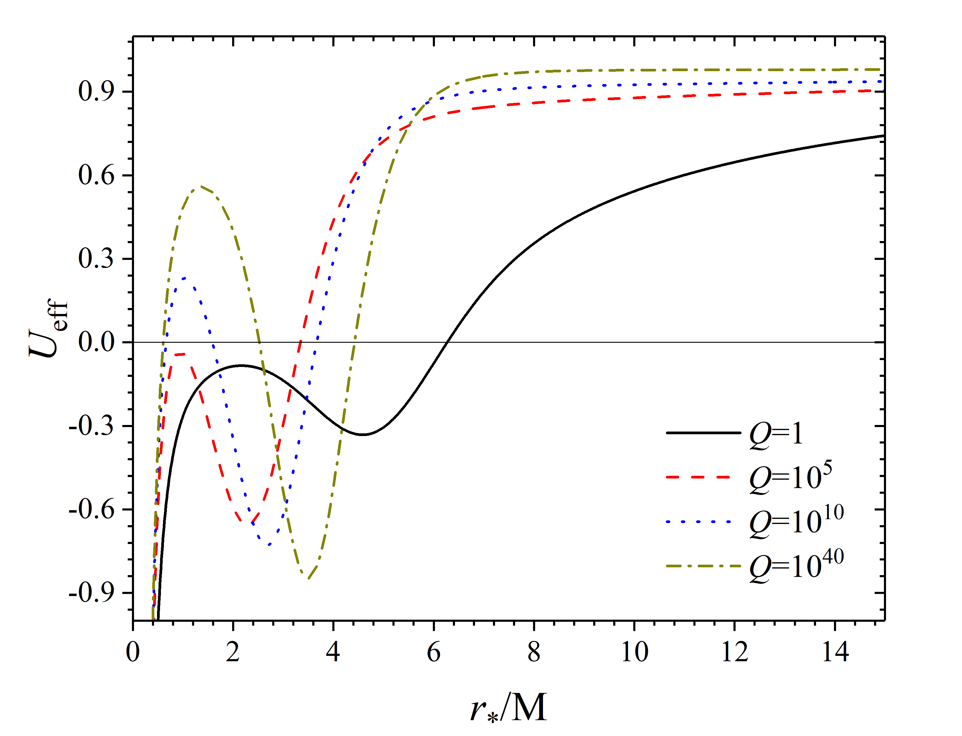
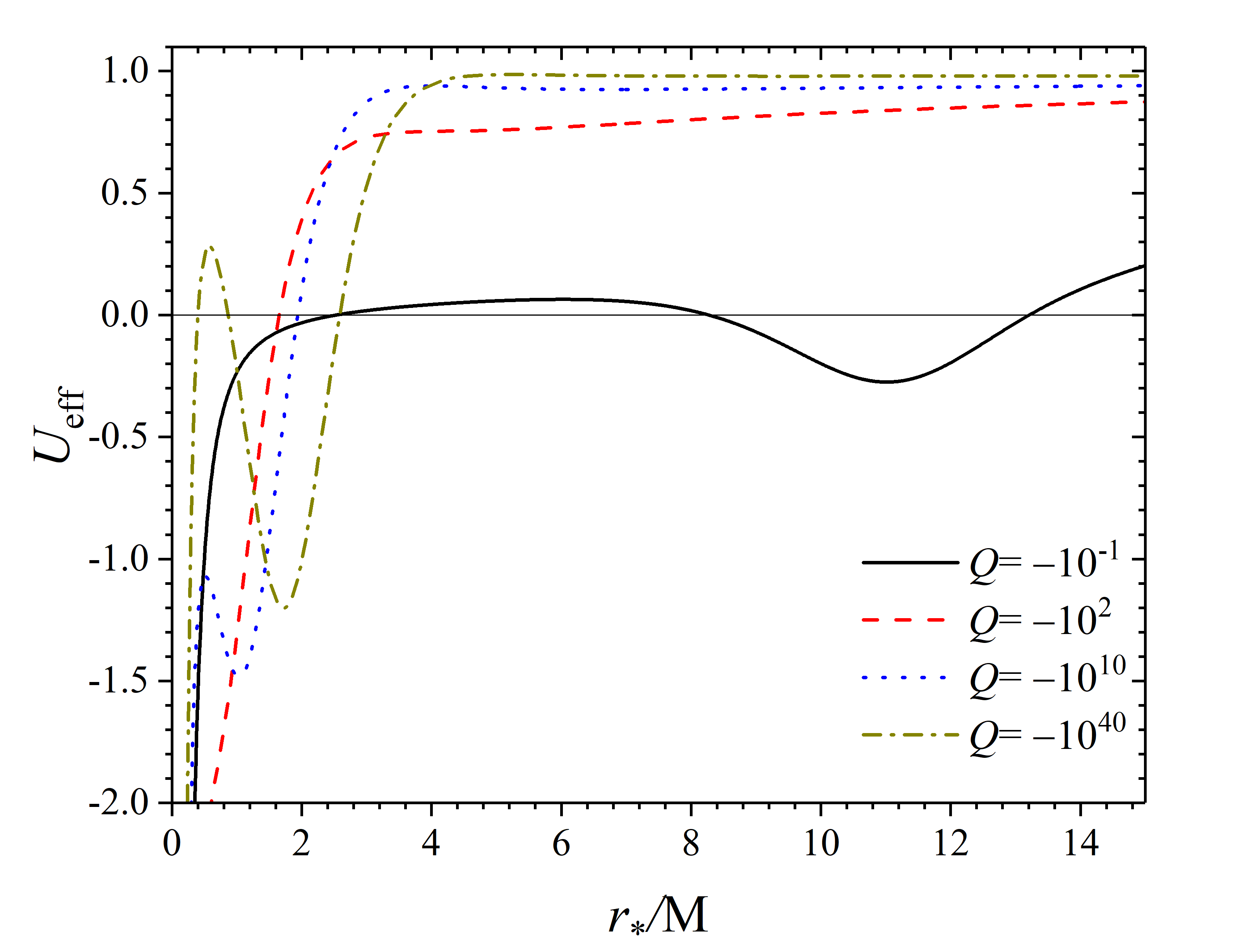
Figure 4: Typical examples of the effective potential $U_{\rm eff}[r(r_{*})]$ for radial perturbations in the case of $M\mu=1$. The upper/lower panel shows the case of positive/negative $Q$. In both cases, $U_{\rm eff}\to\mu^{2}$ as $r_{*}\to\infty$.

Typical examples of $U_{\rm eff}$ are shown in Fig. 4.

The asymptotic behavior of $U_{\rm eff}(r)$ as $r\to 0$ is dominated by the term

$$-\frac{e^{\alpha-\beta}}{r^{2}}\approx\frac{K_{0}}{r^{4}}\left[1+\frac{2\sigma}{\eta+1}\left(\frac{r}{r_{g}}\right)^{\eta+1}\right]\,,\quad$$ (53)

where $K_{0}={X_{0}Y_{0}r_{g}}/{\sigma}$ is not contained in the general asymptotic solution of (50),

$$\Phi(r)=C_{1}\,r+C_{2}\,r\ln r\,,\quad r\to 0\,.$$ (54)

In order that this solution and its derivatives be regular at the origin, we must put $C_{2}=0$; otherwise, the perturbation cannot be considered small. Moreover, if $C_{2}\neq 0$, then the perturbed Kretschmann scalar turns out to be much larger than (46) as $r\to 0$ (cf. [41]).

Therefore, we consider solutions of (50) with regular first derivative at $r=0$ corresponding to

$$\Phi(r)=C_{1}\,r\,,\quad C_{2}=0\,,\quad r\to 0\,.$$ (55)

Another boundary condition is

$$\Phi(r)\to 0,\quad r\to\infty\,.$$ (56)

In terms of the “tortoise” radial variable $r_{*}$ defined as

$$\frac{dr_{*}}{dr}=e^{(\beta-\alpha)/2}\,,\quad r_{*}(0)=0\,,$$ (57)

Eq. (50) can be written in the form

$$\frac{\partial^{2}\Phi}{\partial r_{*}^{2}}-U_{\rm eff}\left[r\left(r_{*}\right)\right]\,\Phi=-\Omega^{2}\Phi\,.$$ (58)

Thus we have the problem of finding an eigenpair $(\Omega^{2},\Phi\in C^{2})$ for the symmetric operator on the left-hand side of (58) with the null Dirichlet boundary condition at the center and condition (56) at infinity. To be precise, we work in the space of $C^{2}$–functions, which are square integrable on $(0,\infty)$. Obviously, the eigenvalues $\Omega^{2}$ of this problem are real; for brevity, we call solutions “unstable” if $\Omega^{2}<0$ and “stable” otherwise.

Note that, for numerical investigations, it is more convenient to deal directly with initial equation (50).

For large values of the radial variable, taking into account (29) and (14), we have

$$W^{\prime\prime}_{\rm eff}(r)\approx\left(1-\frac{r_{g}}{r}\right)\mu^{2}\,,\quad r\to\infty.$$ (59)

The corresponding asymptotic for large $r$ is

$$\Phi(r)\sim D_{1}(\Omega)e^{kr}+D_{2}(\Omega)e^{-kr}\,,\quad k=\sqrt{\mu^{2}-\Omega^{2}}\,.$$

Therefore, a necessary condition for (56) to be satisfied is $\mu^{2}>\Omega^{2}$. The equation for the eigenvalues is

$$D_{1}(\Omega)=0\,,$$ (60)

and it ensures condition (56).

VII Numerical solutions

VII.1 Static SS solutions

We performed backward numerical integration of (24), (25) with respect to $\alpha$, $\beta$, and $\xi$ starting from some sufficiently large value of the radial variable $r_{\text{init}}\gg r_{g}$ and $\mu r_{\text{init}}\gg 1$, where $\xi$ can be assumed sufficiently small and one can use the asymptotic relations (29) to specify the initial conditions. Typically, we chose $r_{\text{init}}=r_{g}+100/\mu$ for moderate $\mu$. We also performed integration of system (35) instead of (24), (25) to test the solutions.

Numerical investigations show that $e^{\alpha(r)}$ is monotonically increasing, while there is a maximum of $e^{\beta(r)}$ at some $r_{\text{max}}$ so that this function is monotonically increasing in the interval $(0,r_{\text{max}})$ and decreasing for $r>r_{\text{max}}$. Near the origin, $e^{\alpha(r)}>e^{\beta(r)}$, but, at some $r=r_{c}$, the sign of the inequality changes and we have $e^{\alpha(r)}<1<e^{\beta(r)}$ for $r>r_{c}$.

As $\mu$ increases, the maximum of $e^{\beta(r)}$ grows and becomes very sharp, whereas, to the left of this maximum, the graphs of $e^{\alpha(r)}$, $e^{\beta(r)}$ are pressed to the abscissa axis. The same situation is observed as $Q$ decreases and becomes small. To the right of the maximum, we have $e^{\alpha(r)}<e^{\beta(r)}$; as $r\to\infty$, these functions tend to the asymptotic value equal to unity. The larger is $\mu$, the faster the asymptotic values are reached.

There are different modes of behavior of $Y(r)$. For fixed $M$ and $\mu$, and for a sufficiently small or negative $Q$, we have $r^{2}W(\xi(r))\leq 1$ for all $r$, and $Y(r)$ is monotonically increasing [see (35b)] with the asymptotics $Y(r)\approx r$ for large $r$. For sufficiently large $Q>0$, we have an interval with negative right-hand side of (35b), where $Y(r)$ is a decreasing function. This interval is bounded because $\xi(r)$ is an exponentially decreasing function and, for sufficiently large $r$, again $r^{2}W(\xi(r))<1$, and $Y(r)$ is monotonically increasing.

Far from the center, SF tends to zero exponentially according to Eq. (29). Moreover, for $Q={\cal O}(1)$ and $M\mu\gg 1$, corresponding to estimate (5), approximation (107) shows that we have practically the Schwarzschild metric already at a distance of several $l_{\mu}$ from $r_{g}$. This, of course, does not mean that, for very large $Q$, the deviations from the Schwarzschild metric cannot be considerable even for $r$ of the order of several $r_{g}$.

Figs. 1 and 2 show the resulting metric coefficients $\tilde{A}(R)$ and $\tilde{B}(R)$ recalculated to the curvature coordinates of the Jordan frame (47). Their behavior is essentially similar to the case of the Einstein frame.

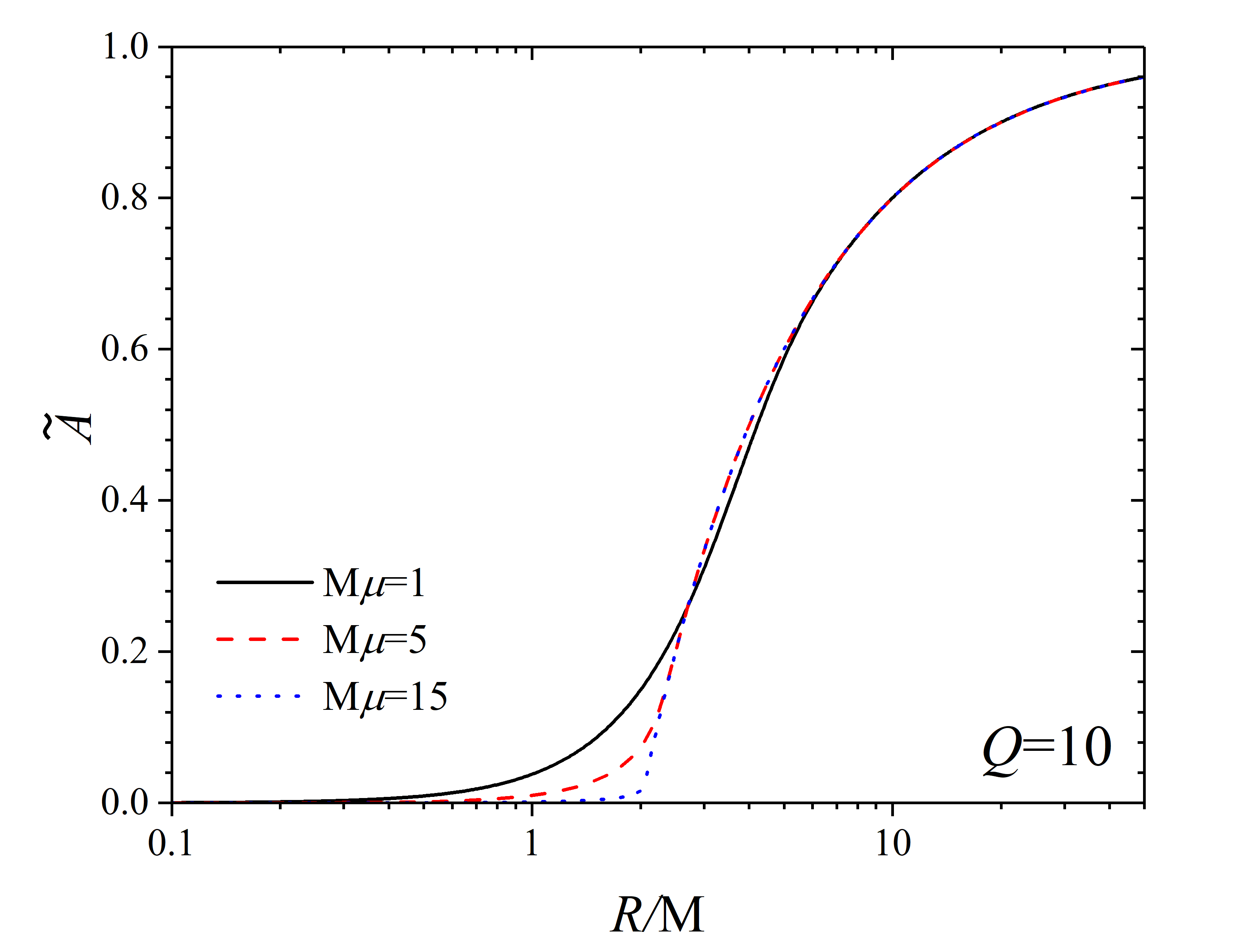
Figure 1: Typical behavior of $\tilde{A}(R)$ in (47) for different values of $M\mu$ and for $Q=10$.

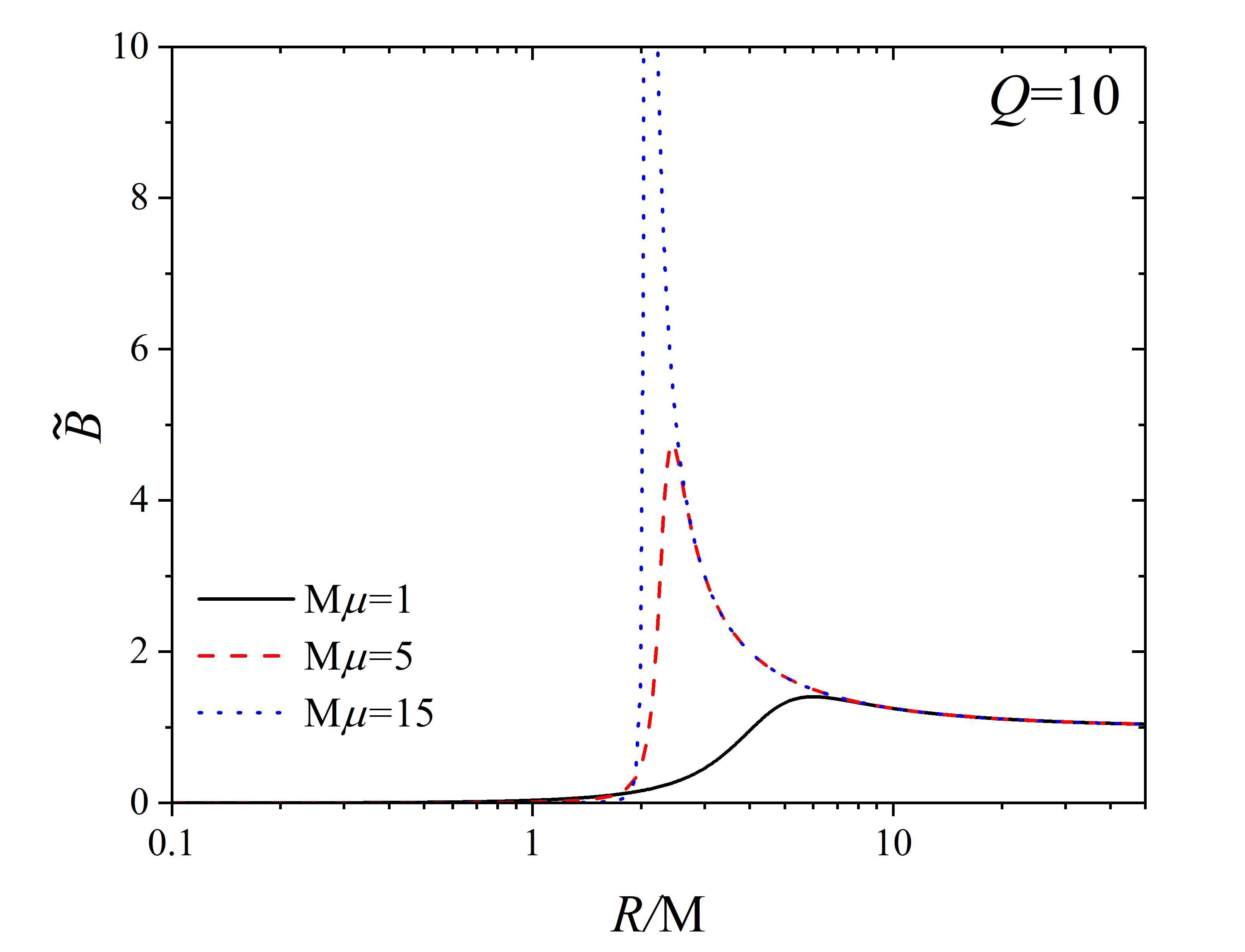
Figure 2: Typical behavior of $\tilde{B}(R)$ in (47) for different values of $M\mu$ and for $Q=10$.

The values $(Y_{0},Z_{0})$ are derived directly from limits (38), (37); this enables us to obtain the parameters $\zeta$ and $\eta$. Figure 3 shows the dependence $\eta(M\mu)$. We also used the functions

$$\tilde{x}(r)=x(r)-\eta\,\ln\left(\frac{r}{r_{g}}\right)\,,\quad\tilde{\xi}(r)=\xi(r)+\zeta\,\ln\left(\frac{r}{r_{g}}\right)\,,$$ (61)

which select the regular parts of $x$ and $\xi$ and enable us to determine

$$x_{0}=\lim\limits_{r\to 0}\tilde{x}(r)\,,\quad\xi_{0}=\lim\limits_{r\to 0}\tilde{\xi}(r)\,,$$ (62)

and then to obtain numerically the parameters $\zeta$, $\eta$, $X_{0}$, $\xi_{0}$, and $\sigma$ as functions of $M\mu$ and $Q$.

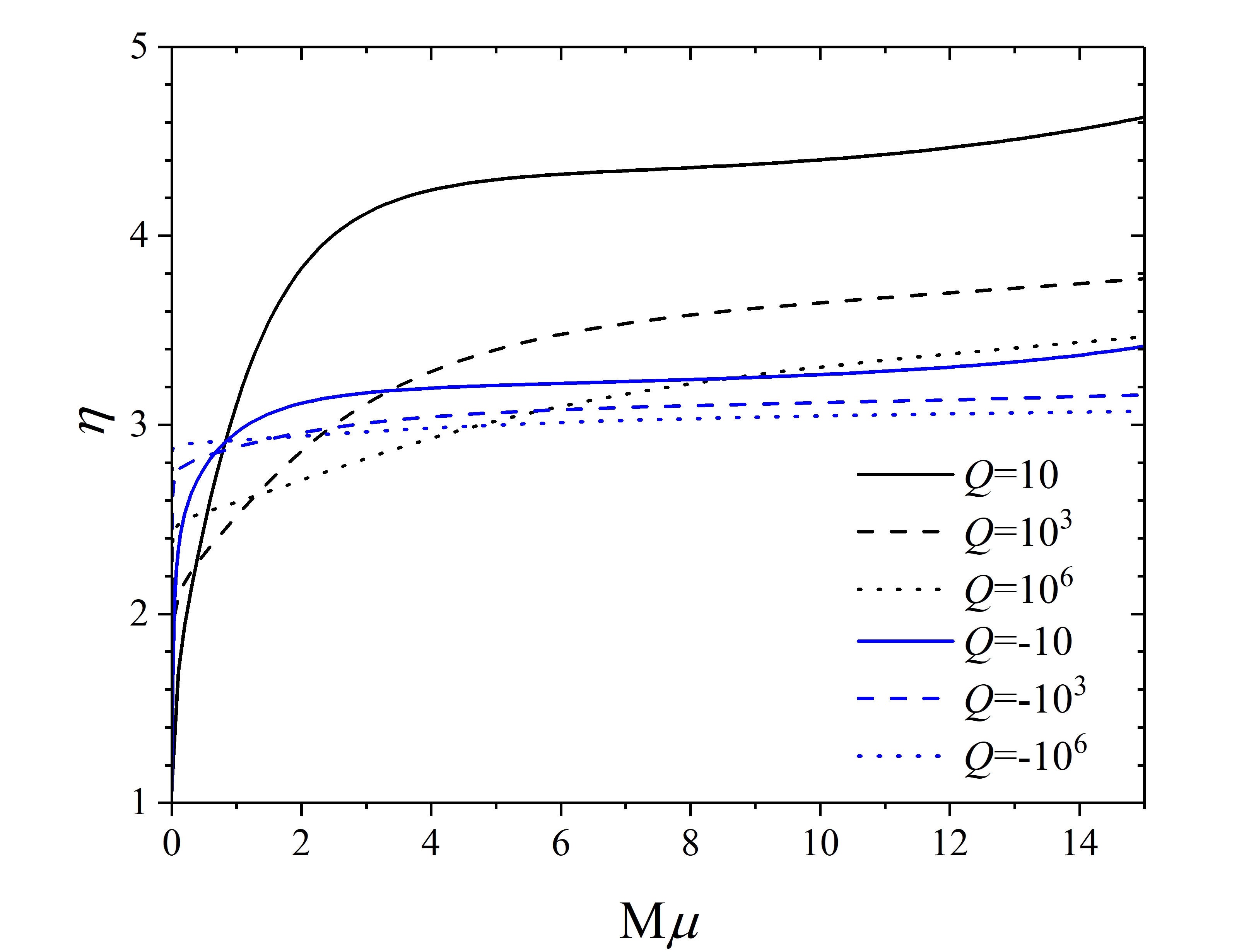
Figure 3: Behavior of $\eta=3\zeta^{2}$ as a function of $M\mu$ for different values of $Q$.

VII.2 (In)stability against radial perturbations

Here we present the results of numerical analysis on linear stability/instability. We imposed null Dirichlet conditions in the center, because otherwise perturbations cannon be considered small. The algorithm of calculations involved two main stages.

• We chose the initial conditions for static SS solutions according to the asymptotic formula (29) at sufficiently large $r$. Next, we performed backward integration of the equations down to the center. Note that this is more convenient than using the shooting method which, in our case, involves four shooting parameters.

• In order to check stability of the static SS solution described by $\alpha$, $\beta$, $\xi$, we considered solutions of the initial-value problem for (50) with initial data according to the asymptotic formula (55) for sufficiently small $r$. We used the shooting method with one shooting parameter $\Omega^{2}$ to check condition (60) yielding the correct asymptotic behavior (56) at infinity. This procedure was carried out for a set of different parameters $(M\mu,Q)$.

In particular, we show that the static SS configurations considered above are linearly unstable at least in some region of parameters. Fig. 5 demonstrates typical dependencies of the eigenvalues $\Omega$ as functions of $Q$. The domains of $(M\mu,Q)$ which correspond to stable and unstable solutions are shown in Fig. 6. Transition to the Jordan frame preserves the time dependence $\sim e^{-i\Omega t}$ and, therefore, the stability/instability domains in Fig. 6.

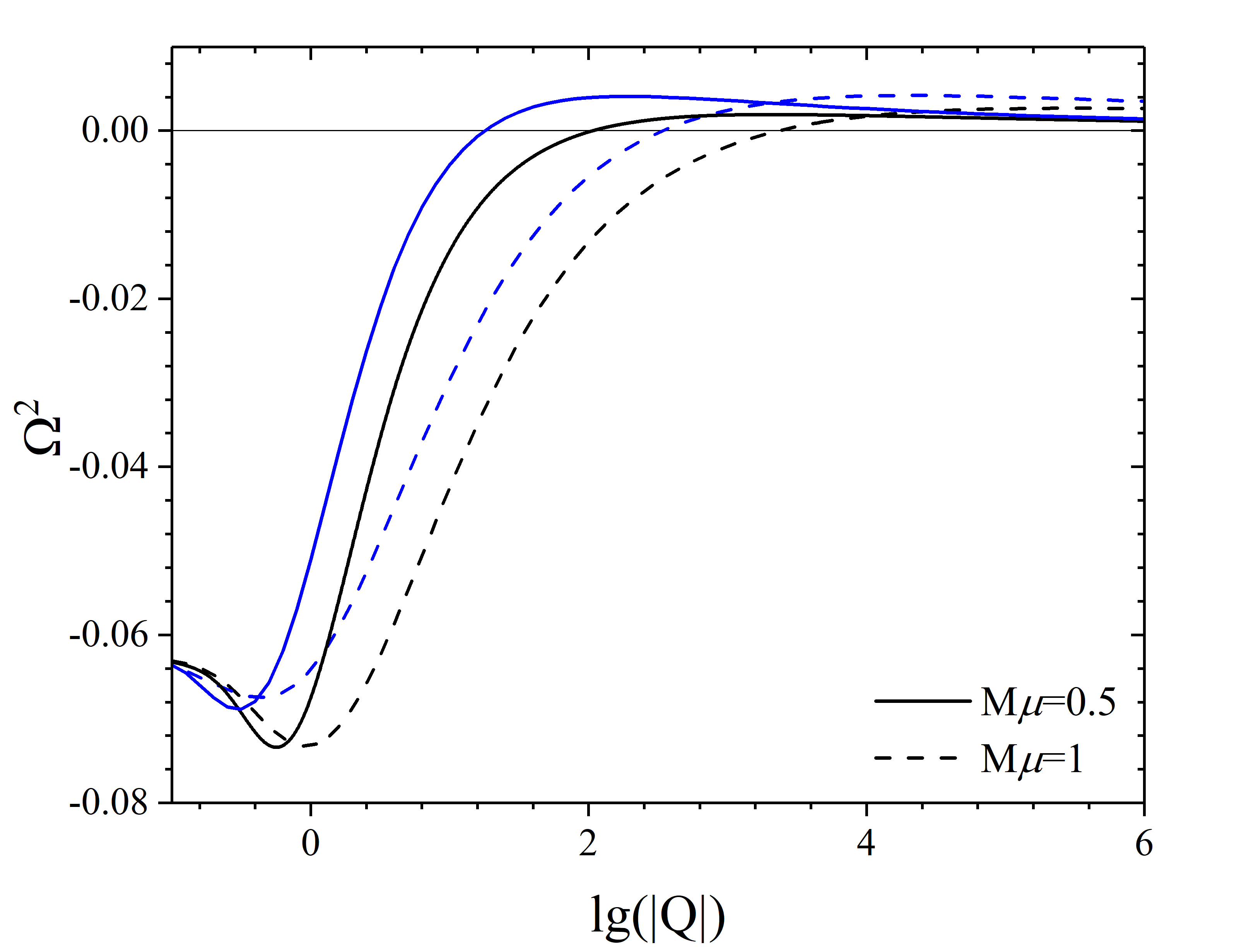
Figure 5: Typical dependencies of $\Omega^{2}(Q)$. Black curves: $Q>0$; blue curves: $Q<0$.

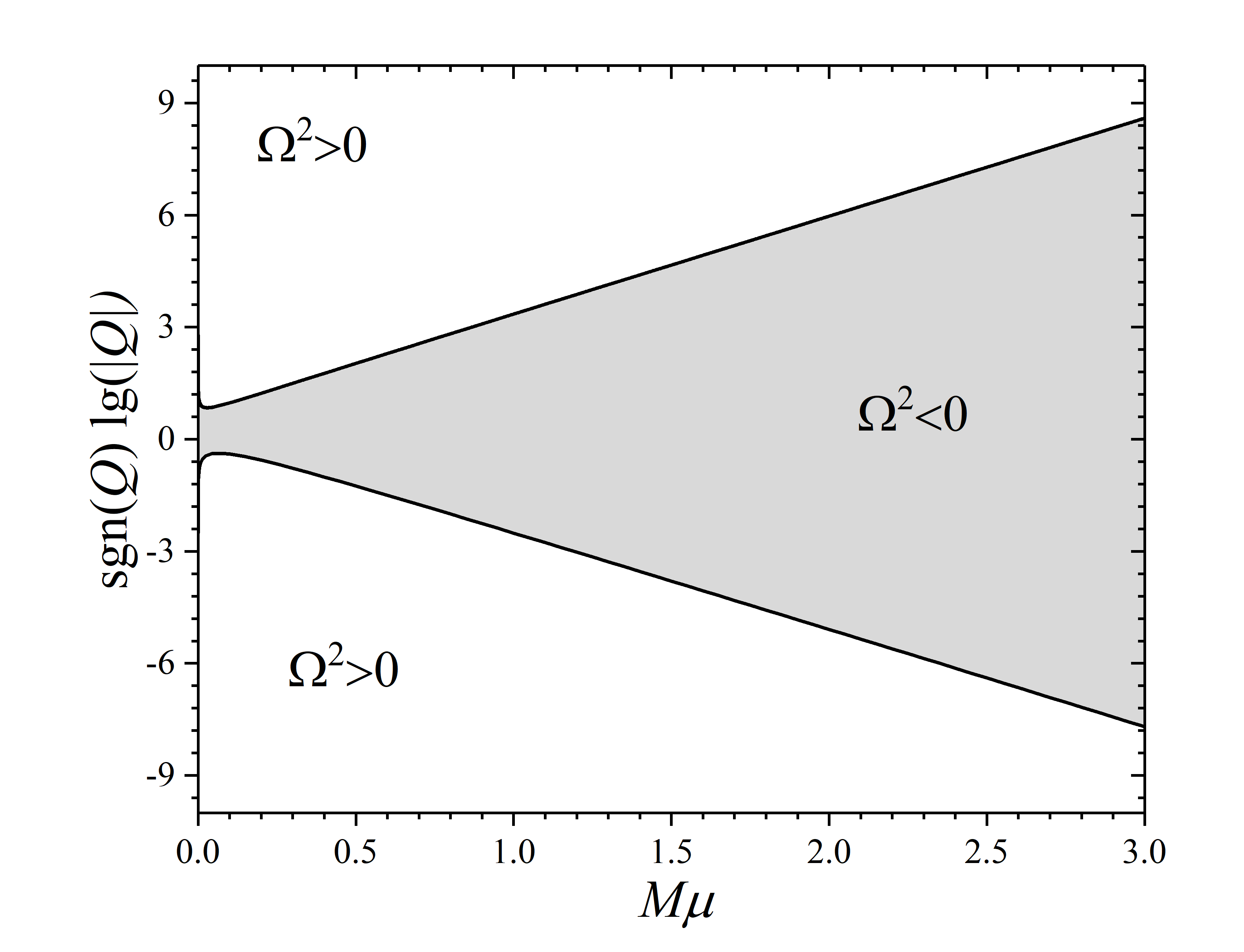
Figure 6: The grey region corresponds to linear instability against radial perturbations of the static SS configurations defined by the parameters $M\mu$ and $Q$. The boundary line corresponds to zero eigenvalues satisfying (60).

VIII Discussion

We studied spherically symmetric configurations of the quadratic $f(R)$ gravity [4]. Transition to the Einstein frame made possible purely analytical treatment of static global solutions using the method of [30]. As follows from our findings, static asymptotically flat SS solutions with zero $T_{\mu\nu}$ are regular outside the center for any scalaron mass and for the global constants $\mathfrak{M}>0$, $Q\neq 0$; they do not have spherical singularities as in case of some configurations with a strongly nonlinear scalar-field potential [44].

In the case of an isolated regular SS structure with a continuous mass-energy distribution in the central region, taking into account the experimental and theoretical bounds on the scalaron mass, the contribution of the scalaron field to the observable effects are expected to be very small. In this case, the gravitational field is determined by the energy-momentum tensor inside the body. Outside the SS body, the field is completely determined by two parameters: the mass $\mathfrak{M}$ and the “scalar charge” $Q$.

Returning to the case of a purely gravitational configuration without ordinary matter ($T_{\mu\nu}\equiv 0$) we state that the parameters $\mathfrak{M}$ and $Q$ act as the only characteristics of the static spherically symmetric system, and there is necessarily a naked singularity at the center if $Q\neq 0$. In this regard, we confirm the statement of [21] concerning the occurrence of NS at the center (although some provisions of this work need adjustment). The only exception is the Schwarzschild solution that corresponds to zero scalaron field ($Q=0$). It is important to note that, whatever small nonzero scalar charge could be, it strongly affects the solution of the quadratic $f(R)$ gravity [4] in the interior region ($r\lesssim r_{g}$) that is visible to an external observer and permeable to external signals moving towards the singularity. Apparently, this situation is typical for many isolated systems with a scalar field, ranging from the linear massless scalar [55, 56] field to configurations with more complicated potentials [30]. No matter how small the scalar field is, it has a strong impact on the properties of spacetime in this region. At the same time, we do not exclude that, for some very large values of $Q$, the deviations from the Schwarzschild metric can be noticeable at distances as large as, say, $r\sim 5$–$10\,r_{g}$. In any case, it is reasonable to defer detailed discussion of the corresponding observational effects until stability issues are resolved.

Our results on the global properties of static SS solutions can be generalized to a wider class of $f(R)$ gravity models. Most restrictive assumption of Section V is the monotonicity requirement (32). From (4) we have

$$W^{\prime}(\xi)=2e^{-4\xi}\left[u\frac{df}{du}-2f(u)\right]\,.$$

Taking into account that $\text{sgn}\,\xi=\text{sgn}\left(f^{\prime}-1\right)$, we have that (32) is satisfied if

$$\left(\frac{df}{du}-1\right)\left(u\frac{df}{du}-2f\right)>0\,.$$

Another restriction deals with the behavior of $|f(u)|$ as $|u|\to\infty$; it must be not faster than $\sim u^{2}$. Possible example is $f(u)=u-u^{2}g(u)$, with $g(u)$ being a bounded rational function such that $g^{\prime}(u)>0$.

In this paper, we were not able to propose a completely analytic treatment of stability, and we used numerical methods. We derived equations for linear perturbations and studied the asymptotic properties of their solutions near the center and for large $r$ with null Dirichlet conditions at the center. We have numerically shown that there are configurations with NS, which are unstable with respect to radial perturbations for a wide range of parameters. Although our numerical simulations involve moderate values of $M$, $Q$, and $\mu$, they suggest that the domain of instability becomes larger for large $M\mu$ so as to include astrophysically interesting values.

On the other hand, there exists the region of parameters where linear perturbations are bounded (the white region in Fig. 6). This could indicate the existence of stable configurations, if not for the following circumstances: (i) in case of a nonlinear system, the existence of bounded linear perturbations does not always mean stability, and nonlinear corrections must be studied (cf., e.g., [41]); (ii) other types of linear perturbations (polar an axial ones) are also possible. In fact, there are general results on the linear stability against axial perturbations leading to a Schrödinger-type equation [57]. One can show that the wave potential in this equation appears to be positive-definite in case of our problem; this can be used to prove stability with respect to axial linear perturbations. However, investigation of polar perturbations is mandatory.

Acknowledgements. O.S. is grateful to Igor Klebanov for kind hospitality at Princeton University. V.I.Z. and Yu.V.S. acknowledge partial support under the scientific program “Astronomy and space physics” of the Taras Shevchenko National University of Kyiv. The work of Yu.V.S. was supported by the Simons Foundation and by the National Academy of Sciences of Ukraine under project 0121U109612.

Appendix A Asymptotic properties as $r\to\infty$

Here we prove the existence of the unique solutions of (23)–(25) with conditions (26), (28); at the same time, our aim is to justify formula (29). The proof uses the standard techniques of the theory of differential equations used in considerations of the conditional stability [58]. The only specific feature of this treatment is that we reduce the problem to integral equations so as to have expressions like (29) in the first iteration.

Introducing a new field variable $\psi=r\xi$ and using (24), we write Eq. (25) for static SF in the form

$$\frac{d^{2}\psi}{dr^{2}}+\left(\frac{d\psi}{dr}-\frac{\psi}{r}\right)\left[\frac{1}{r}\left(1-e^{\beta}\right)+re^{\beta}W(\xi)\right]$$

$$=\frac{r}{6}e^{\beta}W^{\prime}(\xi)\,.$$ (63)

After some rearrangement, we collect the linear part of (63) on the left-hand side:

$$\frac{d^{2}\psi}{dr^{2}}-\left(\frac{d\psi}{dr}-\frac{\psi}{r}\right)\frac{r_{g}}{r(r-r_{g})}-\frac{\mu^{2}\psi}{1-r_{g}/r}$$

$$=F_{1}(r,\alpha,\beta,\psi,d\psi/dr)\,,$$ (64)

where $F_{1}$ contains the nonlinear terms (starting from the second order in $\alpha$, $\beta$, $\psi$, and $d\psi/dr$.

For arbitrary $n=1,2,\ldots$, one can find an asymptotic solution of (64) in the form

$$v(r,\mu)=e^{-\mu r}\left(\frac{r_{g}}{r}\right)^{m}\left(1+\sum_{k=1}^{n}\frac{b_{k}(\mu)}{r^{k}}\right)\,,$$ (65)

$m\equiv m(\mu)=M\mu$, which satisfies the exact relation

$$\frac{d^{2}v}{dr^{2}}-\left(\frac{dv}{dr}-\frac{v}{r}\right)\frac{r_{g}}{r(r-r_{g})}-\frac{\mu^{2}v}{1-r_{g}/r}=\frac{p_{n}(r,\mu)v}{r^{n+2}}\,,$$ (66)

where $p_{n}(r,\mu)$ is a rational function of $r$, bounded as $r\to\infty$; the coefficients $b_{k}$ are determined recursively. In particular, in the case of formula (29), we have $n=2$; the validity of (66) can be checked by direct substitution.

Denote

$$\psi_{1}(r)=v(r,\mu)\,,\quad\psi_{2}(r)=v(r,-\mu)\sim e^{\mu r}\left(\frac{r}{r_{g}}\right)^{m}\,.$$ (67)

The equation for $\psi_{2}$ is obtained from (66) by the change $\mu\to-\mu$. The Wronskian of $\psi_{1}$, $\psi_{2}$ is calculated directly to be $w_{12}=2\mu\left[1+{\cal O}(r^{-1})\right]$.

We use the method of variation of constants by setting

$$\psi(r) =K_{1}(r)\psi_{1}(r)+K_{2}(r)\psi_{2}(r)\,,$$ (68a)

$$\frac{d\psi}{dr} =K_{1}(r)\frac{d\psi_{1}}{dr}+K_{2}(r)\frac{d\psi_{2}}{dr}\,,$$ (68b)

where the “variable constants” are $K_{1}$ and $K_{2}$.

Let $Q_{*}=Qr_{g}$. In order to have the asymptotics $\psi\sim Q_{*}\psi_{1}(r)$ as $r\to\infty$, corresponding to (29), we require

$$K_{1}(\infty)=Q_{*}\,,\quad K_{2}(\infty)=0\,.$$ (69)

A consequence of (68) is

$$\frac{dK_{1}}{dr}\psi_{1}(r)+\frac{dK_{2}}{dr}\psi_{2}(r)=0\,.$$ (70)

Now we differentiate (68b) and substitute the result and Eqs. (68) into (63) using (66). We obtain

$$\frac{dK_{1}}{dr}\frac{d\psi_{1}}{dr}+\frac{dK_{2}}{dr}\frac{d\psi_{2}}{dr}=-G(r,K_{1},K_{2})+F_{1}\,,$$ (71)

where

$$G(r,K_{1},K_{2})=\frac{p_{n}(r,\mu)K_{1}\psi_{1}+p_{n}(r,-\mu)K_{2}\psi_{2}}{r^{n+2}}\,.$$ (72)

Combination of (70) and (71) yields equations for ${dK_{1}}/{dr}$ and ${dK_{1}}/{dr}$. Then, by virtue of (69) and (64),

$$K_{1}(r) =Q_{*}-\int\limits_{r}^{\infty}\frac{G(t)-F_{1}(t)}{w_{12}(t)}\psi_{2}(t)dt\,,$$ (73)

$$K_{2}(r) =\int\limits_{r}^{\infty}\frac{G(t)-F_{1}(t)}{w_{12}(t)}\psi_{1}(t)dt\,.$$ (74)

It is natural to rewrite (23), (24) using the variables

$$x=\frac{\alpha+\beta}{2}\,,\quad y=\frac{\beta-\alpha}{2}+\ln\left(1-r_{g}/r\right)\,.$$ (75)

This gives

$$\frac{dx}{dr} =F_{2}(r,\psi,d\psi/dr)\,,$$ (76)

$$\frac{dy}{dr}+\frac{x+y}{r-r_{g}} =F_{3}(r,x,y,\psi,d\psi/dr)\,,$$ (77)

where the terms nonlinear in $x$, $y$, $\psi$, and $d\psi/dr$ are collected into $F_{2}$ and $F_{3}$. Due to (26), we have

$$x(\infty)=y(\infty)=0\,.$$ (78)

Equations (76), (77) with conditions (78) lead to the integral equations

$$x(r) =-\int\limits_{r}^{\infty}F_{2}(t)dt\,,$$ (79)

$$y(r) =-\int\limits_{r}^{\infty}\left[\frac{(t-r)F_{2}(t)+(t-r_{g})F_{3}(t)}{r-r_{g}}\right]dt\,.$$ (80)

The integral equations (73), (74), (79), (80) can be presented in terms of new variables $u\equiv\{u_{j}\}$, $j=1,\ldots,4$, by means of the following substitutions:

$$K_{1}(r)=u_{1}(r)\,,\quad K_{2}(r)=u_{2}(r)\frac{\psi_{1}(r)}{\psi_{2}(r)}\,,$$ (81)

and

$$x(r)=u_{3}(r)\psi_{1}(r)\,,\quad y(r)=u_{4}(r)\psi_{1}(r)\,.$$ (82)

Accordingly, we have

$$\psi(r) =\left(u_{1}+u_{2}\right)\psi_{1}(r)\,,$$

$$\tilde{G}(r,u) \equiv G(r,K_{1},K_{2})=\frac{p_{n}(r,\mu)u_{1}+p_{n}(r,-\mu)u_{2}}{r^{n+2}}\psi_{1}\,,$$

and the functions

$$\tilde{F}_{j}(r,u)\equiv F_{j}\left(r,x,y,\psi,\frac{d\psi}{dr}\right)\,,\quad j=1,2,3\,,$$

should also be expressed in terms of $u$ by means of (81)–(82).

Introduce the operator $\mathfrak{A}=\{\mathfrak{A}_{1},\mathfrak{A}_{2},\mathfrak{A}_{3},\mathfrak{A}_{4}\}$, where

$$\mathfrak{A}_{1}(r,u) =Q_{*}-\int\limits_{r}^{\infty}\frac{\tilde{G}(t,u)-\tilde{F}_{1}(t,u)}{w_{12}(t)}\psi_{2}(t)dt\,,$$ (83)

$$\mathfrak{A}_{2}(r,u) =\frac{\psi_{2}(r)}{\psi_{1}(r)}\int\limits_{r}^{\infty}\frac{\tilde{G}(t,u)-\tilde{F}_{1}(t,u)}{w_{12}(t)}\psi_{1}(t)dt\,,$$ (84)

$$\mathfrak{A}_{3}(r,u) =-\frac{1}{\psi_{1}(r)}\int\limits_{r}^{\infty}\tilde{F}_{2}(r,u)dt\,,$$ (85)

$$\mathfrak{A}_{4}(r,u) =-\int\limits_{r}^{\infty}\frac{(t-r)\tilde{F}_{2}(t,u)+(t-r_{g})\tilde{F}_{3}(t,u)}{\psi_{1}(r)(r-r_{g})}dt\,.$$ (86)

With this definition, the operator equation

$$u(r)=\mathfrak{A}(r,u)\,,$$ (87)

is equivalent to system (64), (76), (77) with conditions (28) and (78) and, therefore, to the system of equations (23)–(25) with conditions (26), (28). Equation (87) will be considered on interval $[r_{0},\infty)$, where $r_{0}>r_{g}$ will be taken sufficiently large.

Note that

$$|\psi(r)| \leq|u(r)|\psi_{1}(r)\,,$$ (88)

$$\left|\frac{d\psi}{dr}\right| \leq\mu\left[1+{\cal O}(r^{-1})\right]|u(r)|\,\psi_{1}(r)\,,$$ (89)

$$|\tilde{G}(r,u)| \leq\frac{C_{1}}{r^{n+2}}\psi_{1}(r)|u|\,,\quad C_{1}={\cal O}(1)\,,$$ (90)

$|u|=\sum\limits_{i=1}^{4}|u_{i}|$, where we used the explicit expressions (65), (67) and representations (68). Further, we use that, for sufficiently large $r$,

$$\psi_{1}(r)\psi_{2}(r) =1+{\cal O}(r^{-1})\,,$$

$$\int\limits_{r}^{\infty}\psi_{1}^{2}(t)dt =\frac{\psi_{1}^{2}(r)}{2\mu}\left[1+{\cal O}(r^{-1})\right]\,.$$

After some calculations, we see that the functions $\tilde{F}_{j}$ are Lipschitz continuous:

$$|\tilde{F}_{j}(r,u)-\tilde{F}_{j}(r,u^{\prime})|\leq H(u,u^{\prime})|u-u^{\prime}|\,,$$ (91)

where $j=1,2,3$,

$$H(u,u^{\prime})\leq C_{2}\,\max\{|u|,|u^{\prime}|\}\,\psi^{2}_{1}(r)\,,\quad C_{2}={\cal O}(1)\,.$$

Note that we have two small parameters: $\psi_{1}(r)$ and $(r_{g}/r)^{n+1}$; the contribution of the first one (arising due to the nonlinear terms $F_{j}$) in the estimates is exponentially smaller for $r\geq r_{0}$. Then, for sufficiently large $r_{0}$, we have

$$\varepsilon(r_{0})=\max\{(r_{g}/r_{0})^{n+1},\psi_{1}(r_{0})\}=(r_{g}/r_{0})^{n+1}\,.$$

Denote $\|f\|_{a}^{b}\equiv\sup\{f(t),\,t\in[a,b]\}$. Consider the Banach space $\mathcal{B}$ of bounded continuous functions on $[r_{0},\infty)$ with the norm $\|f\|_{r_{0}}^{\infty}$ and a domain $\mathcal{D}\subset\mathcal{B}:\forall u\in\mathcal{D}$, $|u|\leq 2|Q_{*}|$. The operator $\mathfrak{A}$ is well defined on $\mathcal{D}$; all integrals are convergent: in (83), the integrand is estimated as $\sim r^{-{(n+2)}}$ due to (90) and (91); in (84)–(86), we have exponentially decaying expressions in the integrands.

By virtue of the above estimates, we have, for $u\in\mathcal{D}$,

$$|\mathfrak{A}(r,u)|\, \leq\,Q_{*}+C_{3}\varepsilon(r_{0})\|u\|_{r}^{\infty}\,,$$ (92)

$$|\mathfrak{A}(r,u)-\mathfrak{A}(r,v)|\, \leq\,C_{1}\varepsilon(r_{0}){\|u-v\|_{r_{0}}^{\infty}}\,,$$ (93)

where constants $C_{1},C_{3}={\cal O}(1)$. Then from (92) we have that (for sufficiently large $r_{0}$) $\mathfrak{A}(\mathcal{B})\subset\mathcal{B}$ and, from (93), we infer the contraction property. Therefore, equation (87) has a unique solution.

This means that there exists a unique solution $\alpha(r)\in C^{1}$, $\beta(r)\in C^{1}$, $\xi(r)\in C^{2}$ of Eqs. (23)–(25) with conditions (26), (28).

From (83), (84) we infer

$$|\psi(r)-Q_{*}\psi_{1}(r)|=|u_{1}(r)-Q_{*}+u_{2}(r)|\psi_{1}(r)$$

$$\leq\,{\cal O}\bigl{(}r^{-(n+1)}\bigr{)}\psi_{1}(r)\,.$$

This confirms formula (29). Also, using (85), (86), we have

$$|u_{3}(r)|+|u_{4}(r)|\lesssim\psi_{1}(r)\,,$$

whence, on the account of (75),

$$\left|\alpha(r)-\ln\left(1-\frac{r_{g}}{r}\right)\right|+\left|\beta(r)+\ln\left(1-\frac{r_{g}}{r}\right)\right|$$

$$\lesssim{\cal O}\left[\psi^{2}_{1}(r)\right]\,.$$ (94)

Formula (29) is the result of the first iteration of (87). The next iterations add higher-order corrections in powers of $1/r^{n+1}$ and $\exp\,(-\mu r)$, although the latter are useful only if very accurate results are required. In our study, the first iteration yielding (29) and (94) was quite sufficient to impose the initial conditions for backward numerical integration described in Sec. VII.1.

Appendix B The case of $\xi<0$

Here we use the method of [30]. The key question is to prove that the right-hand sides of (35b) and (35c) are bounded as $r\to 0$. If $\xi(r)<0$ for $r\in(0,r_{1})$, then $0<W(\xi)<(3/4)\mu^{2}\exp(4|{\xi}|)$, $|W^{\prime}(\xi)|<3\mu^{2}\exp(4|\xi|)$, and $|\xi(r)|$ is monotonically decreasing due to (35d). For both (35b) and (35c), it is sufficient to estimate

$$P(r)\equiv r^{2}X(r)e^{4|\xi|}=r_{1}^{2}X_{1}e^{4|\xi_{1}|}e^{-2L+4d-(x_{1}-x)}\,,$$ (95)

where $x\equiv x(r)$, $0<r<r_{1}$, and we denoted $x_{1}=x(r_{1})$, $X_{1}=X(r_{1})=\exp(x_{1})$, $\xi_{1}=\xi(r_{1})$, $d(r)=|\xi(r)|-|\xi_{1}|>0$, $L=-\ln(r/r_{1})>0$.

We use the inequality

$$\frac{[\xi(r)-\xi(r_{1})]^{2}}{\ln\left({r_{1}}/{r}\right)}\leq\int\limits_{r}^{r_{1}}t\left(\frac{d\xi}{dt}\right)^{2}dt\,,\quad r<r_{1}\,,$$

which is valid for any continuously differentiable function $\xi$ (see Eq. (31) of [30]). By virtue of (23),

$$x_{1}-x=3\int\limits_{r}^{r_{1}}t\left(\frac{d\xi}{dt}\right)^{2}dt\geq\frac{3}{L}d^{2}\,,$$

where $\xi_{1}\equiv\xi(r_{1})$ . Then

$$-2L+4d-(x_{1}-x)\leq-2L+4d-\frac{3}{L}d^{2}$$

$$=-\frac{3}{L}\left(d-\frac{2}{3}L\right)^{2}-\frac{2}{3}L<0\,,$$

whence

$$P(r)\leq{r_{1}^{2}}X_{1}(r/r_{1})^{2/3}e^{4|\xi_{1}|}\,.$$

This is sufficient to infer the existence of the finite limits $Z_{0}$ and $Y_{0}$ for $\xi(r)<0$.

Appendix C Asymptotic behavior near NS

Here we formulate an iteration procedure to find the asymptotic expansion near NS in curvature coordinates. Taking into account (37) and (38), we have from (35b), (35c)

$$Y(r)=Y_{0}+Y_{1}(r)\,,\quad Z(r)=Z_{0}+Z_{1}(r)\,,$$ (96)

where

$$Y_{1}(r)=\int\limits_{0}^{r}X(t)[1-t^{2}W(\xi(t))]dt={\cal O}\left[r(r/r_{g})^{\eta}\right],$$ (97)

$$Z_{1}(r)=-\frac{1}{6}\int\limits_{0}^{r}t^{2}X(t)W^{\prime}(\xi(t))dt={\cal O}\left[r^{3}\mu^{2}(r/r_{g})^{\eta+2\zeta}\right].$$ (98)

Now we can separate the logarithmic terms in $x$, $\xi$ by setting

$$x(r)=\eta\,\ln\left(\frac{r}{r_{g}}\right)+x_{1}(r)\,,\quad\xi(r)=-\zeta\,\ln\left(\frac{r}{r_{g}}\right)+\xi_{1}(r)\,,$$ (99)

obtaining equations with smooth right-hand sides:

$$\frac{dx}{dr}=\frac{3}{r}D_{1}(r)\,,\quad D_{1}(r)=\frac{Z^{2}}{Y^{2}}-\frac{Z_{0}^{2}}{Y_{0}^{2}}\,,$$ (100)

$$\frac{d\xi_{1}}{dr}=\frac{D_{2}(r)}{r}\,,\quad D_{2}(r)=\frac{Z_{0}}{Y_{0}}-\frac{Z}{Y}\,.$$ (101)

On account of (97), (98), we have $D_{1}(r)={\cal O}\left(r^{\eta+1}\right)$ and $D_{2}(r)={\cal O}\left(r^{\eta+1}\right)$. Then

$$x_{1}(r)=\ln X_{0}+3\int\limits_{0}^{r}\frac{dt}{t}D_{1}(t)\,,\quad\xi_{1}(r)=\xi_{0}+\int\limits_{0}^{r}\frac{dt}{t}D_{2}(t)\,,$$ (102)

$X_{0}>0$ and $\xi_{0}$ being free constants.

Equations (97), (98), (102) with notation (96), (99) form a system of integral equations for the functions $Y_{1}$, $Z_{1}$, $\chi_{1}$, and $\xi_{1}$. This system is ready for successive approximations dealing with well-defined continuous expressions at each step of the iterative procedure that may be used to obtain the asymptotic solution of equations (19)–(22) with four parameters $Y_{0}$, $Z_{0}$, $X_{0}$, and $\xi_{0}$.

The results of the first iterations can be written as follows

$$Y(r)=\ Y_{0}+\frac{X_{0}r_{g}}{\eta+1}\left(\frac{r}{r_{g}}\right)^{\eta+1}\left[1+{\cal O}\left(\mu^{2}r^{2}\right)\right]\,,$$ (103)

$$\chi(r)=\ \eta\,\ln\left(\frac{r}{r_{g}}\right)+\ln X_{0}$$

$${}-\dfrac{2\eta}{(\eta+1)^{2}}\dfrac{r_{g}X_{0}}{Y_{0}}\left(\dfrac{r}{r_{g}}\right)^{\eta+1}\left[1+{\cal O}\left(\mu^{2}r^{2}\right)\right]\,,$$ (104)

$$\xi(r)= -\zeta\,\ln\left(\frac{r}{r_{g}}\right)+\xi_{0}$$

$${}+\dfrac{\zeta}{(\eta+1)^{2}}\dfrac{r_{g}X_{0}}{Y_{0}}\left(\dfrac{r}{r_{g}}\right)^{\eta+1}\left[1+{\cal O}\left(\mu^{2}r^{2}\right)\right]\,,$$ (105)

where $\zeta=Z_{0}/Y_{0}$, $\eta=3\zeta^{2}$.

In case of a spatially flat configuration, the constants $Y_{0}$, $Z_{0}$, $X_{0}$, and $\xi_{0}$ are functions of the pair $M$, $Q$ that uniquely defines the configuration. Having the numerical solutions of Sec. VII, we get $Z_{0}$ of (37), $Y_{0}$ of (38) and $x_{0}$, $\xi_{0}$ of (62). We note a good numerical convergence to these limits.

Returning to the initial variables $e^{\alpha}$, $e^{\beta}$, we obtain the asymptotic formulas (41)–(43).

Appendix D Approximate SF for large $M\mu$ and small $\xi$

As it was pointed out in Sec. III, the realistic values of $M\mu$ must be very large, and we can use the WKB method.

Substitution of $\xi=e^{S}$ into (27) yields

$$\frac{d^{2}S}{dr^{2}}+\left(\frac{dS}{dr}\right)^{2}+\frac{dS}{dr}\frac{d}{dr}\ln\left[r\left({r-r_{g}}\right)\right]=e^{\beta}\mu^{2}\,.$$ (106)

We set

$$S=S_{0}+S_{1}+\ldots\,,\quad|S_{0}|\gg|S_{1}|\,,$$

and we have from (106) the two first orders of this approximation:

$$\xi(r)=\frac{{Q_{1}}\exp\left(-\mu r\sqrt{1-{r_{g}}/{r}}\right)}{(1-{r_{g}}/{r})^{1/4}\left(1+\sqrt{1-{r_{g}}/{r}}\right)^{\mu r_{g}}}\left(\frac{r_{g}}{r}\right)^{1+M\mu},$$ (107)

where we must put $Q_{1}=Q(4/e)^{M\mu}$ so as to have correspondence with (29) for $r\gg r_{g}$. Approximation (107) is effective for $\xi(r)\ll 1$, $\mu\sqrt{r(r-r_{g})}\gg\ln(r/r_{g})$. Note that formula (29), unlike (107), cannot be used for $r$ comparable with $r_{g}$.

References

- Sotiriou and Faraoni [2010] T. P. Sotiriou and V. Faraoni, theories of gravity, Reviews of Modern Physics 82, 451 (2010), arXiv:0805.1726 [gr-qc] .
- De Felice and Tsujikawa [2010] A. De Felice and S. Tsujikawa, theories, Living Reviews in Relativity 13, 3 (2010), arXiv:1002.4928 [gr-qc] .
- Nojiri et al. [2017] S. Nojiri, S. D. Odintsov, and V. K. Oikonomou, Modified gravity theories on a nutshell: Inflation, bounce and late-time evolution, Phys. Rept. 692, 1 (2017), arXiv:1705.11098 [gr-qc] .
- Starobinsky [1980] A. A. Starobinsky, A new type of isotropic cosmological models without singularity, Phys. Lett. B 91, 99 (1980).
- Vilenkin [1985] A. Vilenkin, Classical and quantum cosmology of the Starobinsky inflationary model, Phys. Rev. D 32, 2511 (1985).
- Shtanov et al. [2023] Y. Shtanov, V. Sahni, and S. S. Mishra, Tabletop potentials for inflation from gravity, J. Cosmol. Astroparticle Phys. 03, 023 (2023), arXiv:2210.01828 [gr-qc] .
- Akrami et al. [2020] Y. Akrami et al. (Planck), Planck 2018 results. X. Constraints on inflation, Astron. Astrophys. 641, A10 (2020), arXiv:1807.06211 [astro-ph.CO] .
- Capozziello et al. [2006] S. Capozziello, V. F. Cardone, and A. Troisi, Dark energy and dark matter as curvature effects, J. Cosmol. Astroparticle Phys. 08, 001 (2006), arXiv:astro-ph/0602349 .
- Nojiri and Odintsov [2011] S. Nojiri and S. D. Odintsov, Dark energy, inflation and dark matter from modified gravity, TSPU Bulletin N8(110), 7 (2011), arXiv:0807.0685 [hep-th] .
- Cembranos [2009] J. A. R. Cembranos, Dark matter from gravity, Phys. Rev. Lett. 102, 141301 (2009), arXiv:0809.1653 [hep-ph] .
- Cembranos [2016] J. A. R. Cembranos, Modified gravity and dark matter, J. Phys. Conf. Ser. 718, 032004 (2016), arXiv:1512.08752 [hep-ph] .
- Corda et al. [2012] C. Corda, H. J. Mosquera Cuesta, and R. Lorduy Gomez, High-energy scalarons in gravity as a model for Dark Matter in galaxies, Astropart. Phys. 35, 362 (2012), arXiv:1105.0147 [gr-qc] .
- Katsuragawa and Matsuzaki [2017] T. Katsuragawa and S. Matsuzaki, Dark matter in modified gravity?, Phys. Rev. D 95, 044040 (2017), arXiv:1610.01016 [gr-qc] .
- Katsuragawa and Matsuzaki [2018] T. Katsuragawa and S. Matsuzaki, Cosmic history of chameleonic dark matter in gravity, Phys. Rev. D 97, 064037 (2018), [Erratum: Phys. Rev. D 97, 129902 (2018)], arXiv:1708.08702 [gr-qc] .
- Yadav and Verma [2019] B. K. Yadav and M. M. Verma, Dark matter as scalaron in gravity models, J. Cosmol. Astroparticle Phys. 10, 052 (2019), arXiv:1811.03964 [gr-qc] .
- Parbin and Goswami [2021] N. Parbin and U. D. Goswami, Scalarons mimicking dark matter in the Hu–Sawicki model of gravity, Mod. Phys. Lett. A 36, 2150265 (2021), arXiv:2007.07480 [gr-qc] .
- Shtanov [2021] Y. Shtanov, Light scalaron as dark matter, Physics Letters B 820, 136469 (2021), arXiv:2105.02662 [hep-ph] .
- Shtanov [2022] Y. Shtanov, Initial conditions for the scalaron dark matter, J. Cosmol. Astroparticle Phys. 10, 079 (2022), arXiv:2207.00267 [astro-ph.CO] .
- Holdom and Ren [2017] B. Holdom and J. Ren, Not quite a black hole, Phys. Rev. D 95, 084034 (2017), arXiv:1612.04889 [gr-qc] .
- Kase and Tsujikawa [2019] R. Kase and S. Tsujikawa, Neutron stars in gravity and scalar-tensor theories, J. Cosmol. Astroparticle Phys. 09, 054 (2019), arXiv:1906.08954 [gr-qc] .
- Hernandéz-Lorenzo and Steinwachs [2020] E. Hernandéz-Lorenzo and C. F. Steinwachs, Naked singularities in quadratic gravity, Phys. Rev. D 101, 124046 (2020), arXiv:2003.12109 [gr-qc] .
- Rodrigues-da-Silva and Medeiros [2020] G. Rodrigues-da-Silva and L. G. Medeiros, Spherically symmetric solutions in higher-derivative theories of gravity, Phys. Rev. D 101, 124061 (2020), arXiv:2004.04878 [gr-qc] .
- Bakopoulos and Nakas [2022] A. Bakopoulos and T. Nakas, Analytic and asymptotically flat hairy (ultra-compact) black-hole solutions and their axial perturbations, Journal of High Energy Physics 04, 096 (2022), arXiv:2107.05656 [gr-qc] .
- De Felice and Tsujikawa [2023] A. De Felice and S. Tsujikawa, Stability of Schwarzshild black holes in quadratic gravity with Weyl curvature domination, J. Cosmol. Astroparticle Phys. 10, 004 (2023), arXiv:2307.06490 [gr-qc] .
- De Felice and Tsujikawa [2023] A. De Felice and S. Tsujikawa, Excluding static and spherically symmetric black holes in Einsteinian cubic gravity with unsuppressed higher-order curvature terms, Physics Letters B 843, 138047 (2023), arXiv:2305.07217 [gr-qc] .
- Ye and Wei [2023] X. Ye and S.-W. Wei, Distinct topological configurations of equatorial timelike circular orbit for spherically symmetric (hairy) black holes, J. Cosmol. Astroparticle Phys. 07, 049 (2023), arXiv:2301.04786 [gr-qc] .
- Bekenstein [1972a] J. D. Bekenstein, Transcendence of the law of baryon-number conservation in black-hole physics, Phys. Rev. Lett. 28, 452 (1972a).
- Bekenstein [1972b] J. D. Bekenstein, Nonexistence of baryon number for static black holes, Phys. Rev. D 5, 1239 (1972b).
- Bekenstein [1995] J. D. Bekenstein, Novel “no-scalar-hair” theorem for black holes, Phys. Rev. D 51, R6608 (1995).
- Zhdanov and Stashko [2020] V. I. Zhdanov and O. S. Stashko, Static spherically symmetric configurations with nonlinear scalar fields: Global and asymptotic properties, Phys. Rev. D 101, 064064 (2020), arXiv:1912.00470 [gr-qc] .
- Doneva and Yazadjiev [2020] D. D. Doneva and S. S. Yazadjiev, No-hair theorems for noncanonical self-gravitating static multiple scalar fields, Phys. Rev. D 102, 10.1103/physrevd.102.084055 (2020).
- Bogush et al. [2022] I. Bogush, D. Gal’tsov, G. Gyulchev, K. Kobialko, P. Nedkova, and T. Vetsov, Photon surfaces, shadows, and accretion disks in gravity with minimally coupled scalar field, Phys. Rev. D 106, 024034 (2022), arXiv:2205.01919 [gr-qc] .
- Penrose [1965] R. Penrose, Gravitational collapse and space-time singularities, Phys. Rev. Lett. 14, 57 (1965).
- Penrose [2002] R. Penrose, Gravitational collapse: The role of general relativity, General Relativity and Gravitation 34, 1141 (2002).
- Christodoulou [1984] D. Christodoulou, Violation of cosmic censorship in the gravitational collapse of a dust cloud, Communications in Mathematical Physics 93, 171 (1984).
- Ori and Piran [1987] A. Ori and T. Piran, Naked singularities in self-similar spherical gravitational collapse, Phys. Rev. Lett. 59, 2137 (1987).
- Joshi and Dwivedi [1993] P. S. Joshi and I. H. Dwivedi, Naked singularities in spherically symmetric inhomogeneous Tolman-Bondi dust cloud collapse, Phys. Rev. D 47, 5357 (1993).
- Joshi et al. [2013] P. S. Joshi, D. Malafarina, and R. Narayan, Distinguishing black holes from naked singularities through their accretion disc properties, Classical and Quantum Gravity 31, 015002 (2013).
- Ong [2020] Y. C. Ong, Space–time singularities and cosmic censorship conjecture: A Review with some thoughts, International Journal of Modern Physics A 35, 2030007 (2020).
- Clayton et al. [1998] M. A. Clayton, L. Demopoulos, and J. Légaré, The dynamical stability of the static real scalar field solutions to the Einstein-Klein-Gordon equations revisited, Physics Letters A 248, 131 (1998).
- Gibbons et al. [2005] G. W. Gibbons, S. A. Hartnoll, and A. Ishibashi, On the Stability of Naked Singularities with Negative Mass, Progress of Theoretical Physics 113, 963 (2005), arXiv:hep-th/0409307 [hep-th] .
- Gleiser and Dotti [2006] R. J. Gleiser and G. Dotti, Instability of the negative mass Schwarzschild naked singularity, Classical and Quantum Gravity 23, 5063 (2006), arXiv:gr-qc/0604021 [gr-qc] .
- Dotti [2022] G. Dotti, Linear stability of black holes and naked singularities, Universe 8, 38 (2022).
- Stashko and Zhdanov [2021] O. Stashko and V. I. Zhdanov, Singularities in static spherically symmetric configurations of general relativity with strongly nonlinear scalar fields, Galaxies 9, 72 (2021), arXiv:2109.01931 [gr-qc] .
- Kapner et al. [2007] D. J. Kapner, T. S. Cook, E. G. Adelberger, J. H. Gundlach, B. R. Heckel, C. D. Hoyle, and H. E. Swanson, Tests of the gravitational inverse-square law below the dark-energy length scale, Phys. Rev. Lett. 98, 021101 (2007), arXiv:hep-ph/0611184 .
- Adelberger et al. [2007] E. G. Adelberger, B. R. Heckel, S. A. Hoedl, C. D. Hoyle, D. J. Kapner, and A. Upadhye, Particle-physics implications of a recent test of the gravitational inverse-square law, Phys. Rev. Lett. 98, 131104 (2007), arXiv:hep-ph/0611223 .
- Stelle [1978] K. S. Stelle, Classical gravity with higher derivatives, Gen. Rel. Grav. 9, 353 (1978).
- Perivolaropoulos and Kazantzidis [2019] L. Perivolaropoulos and L. Kazantzidis, Hints of modified gravity in cosmos and in the lab?, Int. J. Mod. Phys. D 28, 1942001 (2019), arXiv:1904.09462 [gr-qc] .
- Asanov [1968] R. A. Asanov, Static scalar and electric fields in Einstein’s theory of relativity, Soviet Journal of Experimental and Theoretical Physics 26, 424 (1968).
- Asanov [1974] R. A. Asanov, Point source of massive scalar field in gravitational theory, Theoretical and Mathematical Physics 20, 667 (1974).
- Rowan and Stephenson [1976] D. J. Rowan and G. Stephenson, The massive scalar meson field in a Schwarzschild background space, Journal of Physics A Mathematical General 9, 1261 (1976).
- Stashko and Zhdanov [2019] O. Stashko and V. Zhdanov, Spherically symmetric configurations in general relativity in the presence of a linear massive scalar field: Separation of a distribution of test body circular orbits, Ukrainian Journal of Physics 64, 189 (2019).
- Chandrasekhar [1998] S. Chandrasekhar, The Mathematical Theory of Black Holes (Oxford University Press, Oxford, UK, 1998).
- Berti et al. [2009] E. Berti, V. Cardoso, and A. O. Starinets, TOPICAL REVIEW: Quasinormal modes of black holes and black branes, Classical and Quantum Gravity 26, 163001 (2009), arXiv:0905.2975 [gr-qc] .
- Fisher [1948] I. Z. Fisher, Scalar mesostatic field with regard for gravitational effects, Zh. Exp. Theor. Phys., 18, 636 (1948), arXiv:gr-qc/9911008 [gr-qc] .
- Janis et al. [1968] A. I. Janis, E. T. Newman, and J. Winicour, Reality of the Schwarzschild singularity, Phys. Rev. Lett. 20, 878 (1968).
- Stashko et al. [2024] O. S. Stashko, O. V. Savchuk, and V. I. Zhdanov, Quasinormal modes of naked singularities in presence of nonlinear scalar fields, Phys. Rev. D 109, 024012 (2024), arXiv:2307.04295 [gr-qc] .
- Coddington and Levinson [1955] E. A. Coddington and N. Levinson, Theory of Ordinary Differential Equations (McGraw-Hill, New York, 1955).