A primary study of CMB delensing for future CMB observations

Abstract

Recognizing the growing significance of contamination from weak gravitational lensing B-modes induced by Large Scale Structure, we investigate a thorough examination of delensing methods aiming at enhancing the sensitivity of $r$ in primordial B-mode detection experiments. In this study, we focus on two specific delensing approaches. One approach involves computing the gradient-order lensing B-mode template by cross-correlating the E-mode with the lensing potential, and subsequently subtracting it from the observed B-mode signal. Another method entails remapping the observations using the estimated deflection angle. Then demonstrate the delensing efficiency using the simulated maps from future CMB polarization experiments, including two ground-based observations: sub-1 m small aperture telescope and 6 m large aperture telescope, and one future space mission with medium aperture telescope. The results reveal that delensing efficiency will be 40% with ground-based small-aperture only, and increases to 65% when combined with a large-aperture telescope. Furthermore, the future satellite experiment achieves an impressive delensing efficiency of approximately 80%.

1 Introduction

The Cosmic Microwave Background (CMB) radiation, originating roughly 380,000 years after the Big Bang, holds invaluable insights into cosmic evolution and serves as a pivotal probe for understanding the early universe. As CMB photons travel freely through space towards us from the last scattering surface, they are subject to gravitational deflection by the large-scale structures (LSS) scattered across the universe. This gravitational influence leads to distortions in the observed pattern of CMB anisotropies. This phenomenon is referred to as the CMB lensing effect, with a characteristic deflection angle typically around $2$ arcminutes.

Weak gravitational lensing, which is a secondary anisotropy on the CMB, has attracted lots interest in recent years. Measurement of the CMB lens provides a rare opportunity to obtain information on the distribution of the cosmic gravitational field, so as to probe the accelerated expansion on large scale, to measure the dark energy equation of state, and to determine the total neutrino mass. Measurements of the lensing potential have been extensively studied in the literature Namikawa et al. (2012), Namikawa & Nagata (2014), Story et al. (2015), Han et al. (2023), Liu et al. (2022). With Planck data release 2013, lensing potential was measured at $25\sigma$ confidence level by the cross correlation of the temperature and polarization maps with LSS of the NVSS, SDSS and WISE cataloguesAde et al. (2016b). With a minimum variance estimator, Planck 2018 temperature and polarization maps improve the measurement of lensing potential to a confidence of 40 $\sigma$Aghanim et al. (2020), and by using the lensing likelihood alone, the combined parameter of matter, $\sigma_{8}\Omega_{m}$ can be measured to an accuracy of a few percent, which is comparable to constraints from galactic lensing. It is worth pointing out that the statistical information from lensing at low redshifts, of galaxy, has a different direction of measurement degeneracy parsimony for $\sigma_{8}\Omega_{m}$ parameter compared to those at high redshifts, of CMB, and thus their combination will be more helpful in improving the measurement accuracy.

Weak gravitational lensing leads to a mixture of the polarization of CMB photon, converting a portion of the primary E-mode into a B-mode. The extra B-modes generating by weak gravitational lensing contaminates the measurements of primordial gravitational waves, so the lensing B-mode is an unavoidable source of intrinsic noise for primordial B-mode detectionManzotti et al. (2017). It is therefore essential to mitigate the lensing B-mode from CMB observation, and a straightforward way is to obtain a specific estimate of the lensing B-mode from the observed map, and then removing it, a process known as "delensing". Delensing procedure becomes critical when the instrumental noise becomes subdominant comparing with the lensed B-mode, which is about $5~{}\mu{\rm K}\cdot{\rm arcmin}$.

The removal of lensing contamination from CMB anisotropy observation maps has received much attention and it has been widely studied in the literatureKesden et al. (2002);Smith et al. (2012);Sherwin & Schmittfull (2015);Simard et al. (2015). The first direct delensing of CMB temperature anisotropies was carried out with taking the cosmic infrared background (CIB) from star-forming dusty galaxies, a linear combination of the 545 and 857GHz maps as the CMB lensing tracer Larsen et al. (2016) , this an external delensing method, and obtain the sharpening of the acoustic peaks of the temperature power spectrum resulting from successful delensing is detected at a significance of $16\sigma$. The first delensing of Planck CMB measurements were performed by an internal delensing, using Planck CMB temperature and polarization measurements themselves to estimate the CMB lensing potential, and then using the estimated deflection map to undo partially the lensing in Carron et al. (2017b) in which they achieved a delensing efficiency of $29\%$ (TT) $25\%$ (TE) and $22\%$ (EE) of the power spectra , and a delensing effects in the B-mode map, with $7\%$ reduction in lensing power. The BICEP/Keck and SPTpol collaborations gave a joint analysis in constraining r by involving lensing template in their likelihood of constraining $r$ Ade et al. (2016a) in 2016, and achieve an improvement on r uncertainty about $10\%$ by adding a lensing B-modes template to their analysis framework in 2021 Ade et al. (2021).

By combining the internal CMB perspective with the cosmic infrared background map from Planck and the galaxy density map from the LSST survey Namikawa et al. (2022), Simons Observatory constructed a template for lensing-induced B-mode for delensing that predicts the contribution of delensing to the $r$ uncertainty. For the next generation ground based CMB observations, CMB-S4, they put lots efforts in developing the delensing procedure to achieve better $r$ constraints. For the target $\sigma(r)\approx 5\cdot 10^{-4}$, the forecast results show that an efficient delensing procedure is an indispensable necessity to achieve high sensitivity. Belkner et al. (2023).

In this paper, we’ll focus on building up delensing procedure, trying to present a delensing framework for ground based CMB polarization observations with the simulated data. The plan of the paper is as follows. In Section 2 we first introduce two delensing methods used in our work, then we thoroughly analyse all the delensing biases. Simulation details of the CMB maps and the lensing potential maps are collected in Section 3. We show our main results of delensing performance in Section 4, and a further analysis with noise debiasing is also performed there, we then give a comparison of two delensing methods. The final conclusion are presented in Section 5. We also derive and prove some algorithms of delensing expression in Appendix A. And the derivation of Wiener filter which is widely used in delensing procedure is given in Appendix B, we also clarify the importance of Wiener filter in delensing procedure there.

2 Delensing Methods

Utilizing the projected gravitational potential, which gives rise to the CMB lensing effect, alongside the observed CMB polarization map, enables us to undertake the delensing. Two main methods are considered in this context: firstly, by creating a gradient-order B-mode template and subtracting it from the observed B-mode, and secondly, employing an inverse-lensing approach. In the latter method, delensing is accomplished by remapping the observed B-mode map using the lensing deflection angle generated by the gravitational potential.

The temperature and polarization anisotropies of lensed CMB are described as:

$$\tilde{\Theta}(\hat{n}) =\Theta(\hat{n}+\nabla\phi(\hat{n}))$$ (1)

$$=\Theta(\hat{n})+\nabla_{i}\Theta(\hat{n})\nabla^{i}\phi(\hat{n})+\mathcal{O}(\phi^{2}),$$

$$(\hat{n}) =[Q\pm iU](\hat{n}+d(\hat{n}))$$ (2)

$$=[Q\pm iU](\hat{n})+\nabla_{i}[Q\pm iU](\hat{n})d^{i}(\hat{n})+\mathcal{O}(\phi^{2}),$$

we exclusively focus on gradient modes, and express the deflection angle $d(\hat{n})$ as the gradient of the lensing potential $d(\hat{n})=\nabla\phi(\hat{n})$ Namikawa & Nagata (2014).

In harmonic space, the E and B-modes can be defined using the spin-2 spherical harmonics ${}_{2}Y_{\ell m}$: Namikawa & Nagata (2014)

$$\begin{gathered}=-\int d\hat{n}_{2}{Y}_{\ell m}(\theta,\phi)\ [Q\pm iU](\hat{n}),\end{gathered}$$ (3)

and the harmonic coefficients of lensing potential $\phi$ are defined as

$$\begin{gathered}\phi_{\ell m}=\int d\hat{n}{Y_{\ell m}}\phi(\hat{n}).\end{gathered}$$ (4)

From Eq.(2), the lensed E and B-modes can be written as Namikawa & Nagata (2014)

$$\begin{gathered}\tilde{E}_{\ell m}=E_{\ell m}+\sum_{\ell^{\prime}m^{\prime}}\sum_{LM}\begin{pmatrix}\ell&\ell^{\prime}&L\\ m&m^{\prime}&M\end{pmatrix}\phi^{*}_{LM}\left\{\mathcal{S}^{(+)}_{\ell\ell^{\prime}L}E^{*}_{\ell^{\prime}m^{\prime}}+i\mathcal{S}^{(-)}_{\ell\ell^{\prime}L}B^{*}_{\ell^{\prime}m^{\prime}}\right\},\end{gathered}$$ (5)

$$\begin{gathered}\tilde{B}_{\ell m}=B_{\ell m}+\sum_{\ell^{\prime}m^{\prime}}\sum_{LM}\begin{pmatrix}\ell&\ell^{\prime}&L\\ m&m^{\prime}&M\end{pmatrix}\phi^{*}_{LM}\left\{\mathcal{S}^{(+)}_{\ell\ell^{\prime}L}B^{*}_{\ell^{\prime}m^{\prime}}-i\mathcal{S}^{(-)}_{\ell\ell^{\prime}L}E^{*}_{\ell^{\prime}m^{\prime}}\right\},\end{gathered}$$ (6)

where $\mathcal{S}^{(\pm)}_{\ell\ell^{\prime}L}$ is given by

$$\mathcal{S}^{(\pm)}_{\ell\ell^{\prime}L} =\frac{(1\pm(-1)^{\ell+\ell^{\prime}+L})}{2}\sqrt{\frac{(2\ell+1)(2\ell^{\prime}+1)(2L+1)}{16\pi}}$$ (7)

$$\times[-(\ell(\ell+1)+\ell^{\prime}(\ell^{\prime}+1)+L(L+1))]\begin{pmatrix}\ell&\ell^{\prime}&L\\ 2&-2&0\end{pmatrix}.$$

2.1 Reconstruct the gradient-order lensing B mode template

Starting from the second line of Eq.(2), we see that the gradient order lensing template can be written as $\nabla_{i}[Q\pm iU](\hat{n})\nabla^{i}\phi(\hat{n})$, the gradient of QU maps and the lensing potential are given by

$$\begin{gathered}\nabla\phi=-\frac{1}{\sqrt{2}}\left\{\sharp\phi\bar{m}+\flat\phi m\right\},\end{gathered}$$ (8)

$$\begin{gathered}\nabla(Q+iU)=-\frac{1}{\sqrt{2}}\left\{\sharp(Q+iU)\bar{m}+\flat(Q+iU)m\right\},\end{gathered}$$ (9)

where we have used the relation of gradient operator defined by Okamoto & Hu (2003)

$$\begin{gathered}D_{i}[{{}_{s}}f(\hat{n})]=-\frac{1}{\sqrt{2}}\left\{\sharp{{}_{s}}f(\hat{n})\bar{m}+\flat{{}_{s}}f(\hat{n})m\right\},\end{gathered}$$ (10)

where $\sharp$ and $\flat$ are the ladder operators, $D_{i}$ is the gradient operator, ${{}_{s}}f(\hat{n})$ is a spin-s function and complex-conjugated vectors $\bar{m}$ and $m$ have the property

$$\begin{gathered}m\cdot m=\bar{m}\cdot\bar{m}=0,\quad m\cdot\bar{m}=1,\end{gathered}$$ (11)

Given QU maps and a potential map, our initial step involves decomposing them into harmonic coefficients of E and B-modes. We prioritize E-modes due to their significantly higher strength compared to B-modes, thus neglecting any leakage from B-modes to E-modes. Subsequently, we transfer E-modes into a spin-1 field and a spin-3 field using ladder operators. Additionally, we transform the potential map into spin-1 and spin-$-1$ fields through the operation as follows:

$$\begin{gathered}\sharp(Q+iU)=\sum_{\ell m}\sqrt{(\ell+3)(\ell-2)}E_{\ell m}{{}_{3}}Y_{\ell m},\end{gathered}$$ (12)

$$\begin{gathered}\flat(Q+iU)=-\sum_{\ell m}\sqrt{(\ell+2)(\ell-1)}E_{\ell m}{{}_{1}}Y_{\ell m},\end{gathered}$$ (13)

$$\begin{gathered}\sharp\phi=\sum_{\ell m}\sqrt{\ell(\ell+1)}\phi_{\ell m}{{}_{1}}Y_{\ell m},\end{gathered}$$ (14)

$$\begin{gathered}\flat\phi=-\sum_{\ell m}\sqrt{\ell(\ell+1)}\phi_{\ell m}{{}_{-1}}Y_{\ell m},\end{gathered}$$ (15)

where $Q$ and $d^{R}$ represent the real part of a field, and $U$ and $d^{I}$ represent the imaginary part of a field.

No B-mode should be included in Eq.(12) and Eq.(13), as introducing B-mode would intuitively imply that its presence will undergo lensing to the same order as the lensing B-mode (as Eq.(6)). Following this consideration, we proceed to calculate the gradient order lensing template as follows:

$$\nabla_{i} [Q\pm iU](\hat{n})\nabla^{i}\phi(\hat{n})$$ (16)

$$=\frac{1}{2}\left\{\sharp\phi\bar{m}+\flat\phi m\right\}\left\{\sharp(Q+iU)\bar{m}+\flat(Q+iU)m\right\}$$

$$=\frac{1}{2}[(d^{1,R}+id^{1,I})(Q^{1}+iU^{1})+(d^{1,R}-id^{1,I})(Q^{3}+iU^{3})],$$

where in the last line the index on top-right represent the spin of a field. Separate the real and imaginary part, we have

$$\begin{gathered}Q=\frac{1}{2}[d^{1,R}(Q^{1}+Q^{3})-d^{1,I}(U^{1}-U^{3})],\end{gathered}$$ (17)

$$\begin{gathered}U=\frac{1}{2}[d^{1,R}(U^{1}+U^{3})+d^{1,I}(Q^{1}-Q^{3})].\end{gathered}$$ (18)

The lensing B-mode template can be derived from the lensing QU maps, and the delensed B-mode is obtained by subtracting the template map from the observed B-mode map. In practice, we utilize the lensed QU maps rather than the unlensed ones, as the former facilitates a cancellation between the low-order terms in the delensed power spectrum, unlike the latter, as described in Baleato Lizancos et al. (2021).

2.2 Inverse-lensing method

The second delensing method is more straightforward. From Eq.(1) and Eq.(2), we understand that the lensing effect can be reversed by remapping the observed photons back to their original positions. Therefore, the original unlensed field can be recovered by remapping the lensed field with an inverse deflection angle. The inverse deflection angle can be well defined because the points are remapped onto themselves after being deflected back and forth, as detailed in Diego-Palazuelos et al. (2020).

$$\begin{gathered}\hat{n}+\beta(\hat{n})+\alpha(\hat{n}+\beta(\hat{n}))=\hat{n},\end{gathered}$$ (19)

and the unlensed field can be recovered from the lensed field by remapping the lensed field with an inverse deflection angle:

$$\begin{gathered}\tilde{X}(\hat{n})=X(\hat{n}+\alpha(\hat{n}))\Leftrightarrow X(\hat{n})=\tilde{X}(\hat{n}+\beta(\hat{n})).\end{gathered}$$ (20)

Eq.(19) can be solved adopting a Newton-Raphson scheme, the inverse deflection angle $\beta(\hat{n})$ can be iteratively calculated through Carron et al. (2017a)

$$\begin{gathered}\beta_{(i+1)}(\hat{n})=\beta_{(i)}(\hat{n})-M^{-1}(\hat{n}+\beta_{(i)}(\hat{n}))\cdot[\beta_{(i)}(\hat{n})+\alpha(\hat{n}+\beta_{(i)}(\hat{n}))],\end{gathered}$$ (21)

where $M(\hat{n})$ is the magnification matrix, defined from the sphere’s metric $g_{ab}$, as

$$\begin{gathered}M_{ab}(\hat{n})=g_{ab}+\nabla_{a}\alpha_{b}(\hat{n}).\end{gathered}$$ (22)

We can then remap the observed map with the estimated inverse deflection angle in order to estimate the original map.

2.3 Delensing Bias

In this section, we will examine the biases introduced by the delensing procedure and propose methods for their correction.

Debiasing is necessary for obtaining an accurate measurement of $r$. We assert that the biases we express below are not the delensing biases arising from the overlap in modes between the B-field to be delensed and the B-field used to reconstruct the lensing potential, as discussed in references such as Lizancos et al. (2021) and Teng et al. (2011), where a disconnected four point function appeared due to the overlap when calculating the power spectrum of the delensed B-mode, which is proven to wrongly underestimate the delensed B power. In our subsequent derivation, we solely focus on separating each component contributing to the delensing residuals (biases), without considering the B-mode overlap mentioned above.

2.3.1 Analysis of Biases in the Gradient-Order Template Method

The observed E and B modes with Wiener-filter (for a detailed description, please refer to 4.1.) are as follows:

$$E=\mathcal{W}^{E}(E^{lens}+E^{noise}),$$ (23)

$$B=\mathcal{W}^{E}(B^{lens}+B^{noise}),$$

$$\hat{\phi}=\mathcal{W}^{\phi}(\phi+\phi^{noise}).$$

For the gradient order template method, we calculate the gradient of the lensing B-modes template according to Eq.(2), then using Eq.(47), and get:

$$B^{temp} =\mathcal{B}^{(1)}[\mathcal{W}^{E}(E^{lens}+E^{noise})\ast\mathcal{W}^{\phi}(\phi+\phi^{noise})]$$ (24)

$$=\begin{aligned} &\left\{\mathcal{B}^{(1)}[\mathcal{W}^{E}E^{lens}\ast\mathcal{W}^{\phi}\phi]\right\}+\mathcal{B}^{(1)}[\mathcal{W}^{E}E^{noise}\ast\mathcal{W}^{\phi}\phi]\\ &+\mathcal{B}^{(1)}[\mathcal{W}^{E}(E^{lens}+E^{noise})\ast\mathcal{W}^{\phi}\phi^{noise}]\end{aligned}$$

$$=B^{temp}_{S}+B^{temp}_{N}.$$

Here $\mathcal{B}^{(1)}[E\ast\phi]$ represents the operation of constructing the gradient order template with $E$ and $\phi$. We artificially define the signal part ($B^{temp}_{S}$) which consists of the signal (the term in the brace), and the noise part ($B^{temp}_{N}$) introduced during the delensing procedure.

Furthermore, we recognize that $B^{temp}_{S}$ does not solely represent the pure lensing B-modes; rather, it constitutes a filtered version of the lensing B-modes. In fact, a bias is introduced by the Wiener filter, and certain high-order terms are neglected when constructing the template. Therefore, we express $B^{temp}_{S}$ as:

$$\begin{gathered}B^{temp}_{S}=B^{lens}+N^{\prime},\end{gathered}$$ (25)

where $N^{\prime}$ denotes the bias induced by both the Wiener filter and the method itself. This bias can be understood from Eq.(6), where the gradient-order template is a good approximation on large scales. However, with increasing $\ell$, the higher-order terms of the lensing B-modes become more significant. Therefore, the neglect of these high-order terms contributes to the bias, particularly on small scales. We denote $N^{\prime}$ as the intrinsic bias to distinguish it from the noise part, as this term persists even when delensing with a noiseless map.

Then the delensed B-modes can be written as:

$$B^{del} =B^{obs}-B^{temp}$$ (26)

$$=(B^{lens}+B^{noise})-(B^{lens}+N^{\prime}+B^{temp}_{N})$$

$$=B^{noise}-N^{\prime}-B^{temp}_{N}.$$

Therefore, there are three components contributing to the delensed B-modes: the delensing residual $N^{\prime}$, the intrinsic noise in observed B-modes, and the noise introduced during the delensing procedure. We denote the latter two as the delensing noise.

2.3.2 Bias analysis of inverse-lensing method

The inverse-remapped B-mode can be written as (check 47):

$$B^{del} =\mathcal{B}[\mathcal{W}^{E}(B^{lens}+B^{noise})\star\beta]$$ (27)

$$\approx\mathcal{B}[\mathcal{W}^{E}(B^{lens}+B^{noise})\star(\beta_{\phi}+\beta_{noise})]$$

$$\approx\left\{\mathcal{B}[\mathcal{W}^{E}B^{lens}\star\beta_{\phi}]\right\}$$

$$+\left\{\mathcal{B}[\mathcal{W}^{E}B^{lens}\star\beta_{noise}]+\mathcal{B}[\mathcal{W}^{E}B^{noise}\star\beta]-\mathcal{W}^{E}B^{lens}\right\}$$

$$=B^{del}_{S}+B^{del}_{N},$$

Here, $\mathcal{B}[B\star\phi]$ represents the delensing operation of lensing B mode with $\phi$ to obtain the delensed B-modes. Here, $B^{del}_{S}$ includes the delensed B signal (the first brace), which is the desired output and arises from the method itself, therefore exists even under noiseless observation. While $B^{del}_{N}$ represents the noise part arising from intrinsic noise and noise introduced by the delensing procedure.

The lensing template B-mode is then:

$$B^{temp} =B^{obs}-B^{de}$$ (28)

$$=[B^{lens}+B^{noise}]-[B^{de}_{S}+B^{de}_{N}]$$

$$=[B^{lens}-B^{de}_{S}]+[B^{noise}-B^{de}_{N}]$$

$$=B^{temp}_{S}+B^{temp}_{N},$$

Where $B^{temp}_{S}$ encompasses the lensing template B-mode we aim to obtain, and $B^{temp}_{N}$ represents the noise component. It’s important to note that $B^{temp}_{S}$ still retains an intrinsic bias.

$$B^{temp}_{S}=B^{lens}-B^{del}_{S},$$ (29)

Where the bias $B^{del}_{S}$ arises from the approximation introduced in obtaining the inverse-lensing angle, and we denote it as the intrinsic bias to distinguish it from the noise bias.

2.3.3 The impact of delensing bias on $r$ constraint

The observed B-modes and delensed B-modes can be written as:

$$B^{obs} =B^{tens}+B^{lens}+B^{noise},$$ (30)

$$B^{del} =B^{tens}+B^{res}+B^{del}_{N}+B^{noise}.$$

Where $B^{del}$ represents the noisy delensed B-modes we construct, $B^{lens}$ is the lensing B-modes, $B^{tens}$ is the true unlensed B-modes from tensor fluctuations we seek, $B^{res}$ denotes the lensing residual, $B^{del}_{N}$ denotes the noise introduced during the delensing procedure (delensing noise), and $B^{noise}$ represents the intrinsic noise of the observed lensed B-modes.

The BB angular power spectra without and with delensing can be written as:

$$C_{\ell}^{obs} =C_{\ell}^{tens}+C_{\ell}^{lens}+N_{\ell}^{BB},$$ (31)

$$C_{\ell}^{del} =C_{\ell}^{tens}+C_{\ell}^{res}+N_{\ell}^{del}+N_{\ell}^{BB}.$$

Here we define the delensing fraction as:

$$\begin{gathered}f_{dl}=(C_{\ell}^{res}+N_{\ell}^{del})/C_{\ell}^{lens}.\end{gathered}$$ (32)

For cases without delensing, $f_{dl}=1$. Then the BB angular power spectra without and with delensing can be simplified as:

$$\begin{gathered}C_{\ell}=C_{\ell}^{tens}+f_{fl}C_{\ell}^{lens}+N_{\ell}^{BB}.\end{gathered}$$ (33)

When fitting the tensor-to-scalar ratio ($r$) using the angular power spectra, we often utilize the following parameterization:

$$\begin{gathered}C_{\ell}=rC_{\ell}^{tens}(r=1)+A_{L}C_{\ell}^{len,th}+N_{\ell}^{BB}.\end{gathered}$$ (34)

$C_{\ell}^{len,th}$ represents the lensing BB spectra from the theory, and $A_{L}$ is a constant characterizing the lensing amplitude. $N_{\ell}^{BB}$ is estimated from the observed B modes noise only simulations. When we do not perform the delensing operation, $A_{L}$ is approximately equal to 1, and the estimation of $r$ is unbiased. During delensing, if $f_{dl}$ is independent of $\ell$, the estimation of $r$ remains unbiased. Typically, $A_{L}<1$. However, if $f_{dl}$ heavily depends on $\ell$, we need to adjust the parameterization to:

$$\begin{gathered}C_{\ell}=rC_{\ell}^{tens}(r=1)+A_{L}C_{\ell}^{len,th}+N_{\ell}^{del}+N_{\ell}^{BB}.\end{gathered}$$ (35)

The estimation of $N_{\ell}^{del}$ is obtained from simulations.

The uncertainty of $r$ can be roughly expressed as:

$$\begin{gathered}\sigma(r=0)=\left[\sum_{l}\frac{(2l+1)f_{sky}}{2}\left(\frac{C_{l}^{tens}(r=1)}{f_{dl}C_{l}^{len}+N_{l}^{BB}}\right)^{2}\right]^{-1/2}.\end{gathered}$$ (36)

From Eq.36, it can be observed that the uncertainty in $r$ decreases as $f_{dl}$ decreases. This reduction in uncertainty is the motivation behind performing the delensing operation.

3 Data simulation

We utilize simulated data to illustrate the feasibility of delensing methods. We simulate far future CMB polarization observations from various experiments, including one medium-aperture satellite mission of $3m$ telescope (sMAT), one small-aperture ground based $80cm$ telescope(gSAT), and one ground $6m$ large-aperture telescope (gLAT), to predict the delensing efficiency of different experiments and methods. This paper focuses on the study of delensing methods, and we do not consider the influence of foregrounds. In our next article, we will investigate the impact of foregrounds on delensing and its effect on the tensor-to-scalar ratio $r$ for a more realistic simulation.

The input unlensed CMB maps are Gaussian realizations generated from a specific power spectrum obtained from the Boltzmann code CAMB Lewis & Challinor (2011), using the Planck 2018 best-fit cosmological parameters Aghanim et al. (2020) with the tensor scalar ratio $r=0$. We then utilize the Lenspyx package, which implements an algorithm to distort the primordial signal given a realization of the lensing potential map from $C_{\ell}^{\phi\phi}$. The lensed CMB maps are smoothed by the instrumental beam sizes listed in Table 1 respectively. All the maps are in the HealPix pixelization scheme at $\texttt{NSIDE}=2048$. The noise in the sky patch is homogeneous with noise levels listed in Table 1. Finally, we add the smoothed lensed CMB maps with noise maps, and then multiply them by the sky patch masks to produce simulated observed maps for 3 experiments.

Table 1: The parameters of the three experiments

Experiment	$\theta_{\text{FWHM}}$	$\sigma_{\text{noise}}$	$f_{\text{sky}}$	$\ell range$
gLAT	1.4 arcmin	6.0 $\mu K\cdot arcmin$	0.1	(300,5000)
gSAT	11.6 arcmin	2.0 $\mu K\cdot arcmin$	0.1	(30,1000)
sMAT	2.8 arcmin	1.5 $\mu K\cdot arcmin$	0.8	(2,3800)

4 Delensing implementation and Results

In this section, we first describe our implementation of delensing, then we present our main results of delensing and some further results after noise debiasing. Fig. 1 shows our flowchart of the delensing pipeline.

Figure 1: Flowchart of the delensing pipeline. We separate our pipeline into four parts: map simulation, lensed CMB maps processing, lensing potential processing and the implementation of two delensing methods.

4.1 Lensed CMB maps processing

We initially perform Wiener-filter on the observed QU maps to enhance the signal-to-noise ratio (SNR) prior to delensing, as follows:

$$\begin{gathered}Q_{\ell m}\Rightarrow\frac{C_{\ell}^{EE}}{C_{\ell}^{EE}+N_{\ell}^{EE}}Q_{\ell m},\\ U_{\ell m}\Rightarrow\frac{C_{\ell}^{EE}}{C_{\ell}^{EE}+N_{\ell}^{EE}}U_{\ell m}.\\ \end{gathered}$$ (37)

We provide a thorough derivation and clarification of the Wiener filter in the delensing operation in Appendix B.

For combining experiments, we will initially perform map combination using the inverse-variance method:

$$\chi_{\ell m}=\sum_{i}\omega_{i,\ell}\chi_{i,\ell m},$$ (38)

$$\omega_{i,\ell}=\frac{N_{i,\ell}^{-1}}{\sum_{i}N_{i,\ell}^{-1}}.$$

Here, $\omega_{i,\ell}$ represents the weights of the $i$th experiment, $N_{i,\ell}$ is the noise power spectrum of the $i$th experiment after beam deconvolution, $\chi_{i,\ell m}$ denotes the harmonic coeffcients of fields of the $i$th experiment after beam deconvolution, and $\chi_{\ell m}$ represents the combined alm.

Next, we perform Wiener-filter on the combined maps, as mentioned above, and the combined E-mode noise power spectrum is given by:

$$N_{\ell}^{EE}=\sum_{i}\omega_{i,\ell}^{2}N_{i,\ell}^{EE}.$$ (39)

4.2 Lensing potential reconstruction

In realistic situations, the lensing potential can be constructed either from internal datasets, such as the observed QU maps, or from external datasets like the large-scale structure. However, for the purposes of this discussion, we will only focus on the delensing process. Therefore, we will simply use the provided $\phi$ map with reconstruction noise, which is realized from the $N_{l}^{\phi\phi}$ given by the quadratic estimator:

$$\begin{gathered}N^{(0),\alpha\alpha}_{L}=A^{\alpha}_{L}=(2L+1)\left\{\sum_{l_{1}l_{2}}\frac{|f_{l_{1}Ll_{2}}^{\alpha}|^{2}}{2C_{l_{1}}^{aa}C_{l_{2}}^{bb}}\right\}^{-1}\end{gathered}$$ (40)

where "a" means one CMB field among $\Theta$, E, B, and $\alpha$ represents a pair of CMB field used for estimator, $f_{l_{1}Ll_{2}}^{\alpha}$ is the weight for the different quadratic pairs Okamoto & Hu (2003) , and $C_{l_{1}}^{aa}$ is the auto- power spectrum of a CMB field among $\Theta$, E, B. The noise spectra for different experiments are shown in Figure 2. One can see that combining the gSAT with gLAT leads to a reduction in reconstruction noise thanks to the extension in small-scale coverage and the suppression of instrument noise.

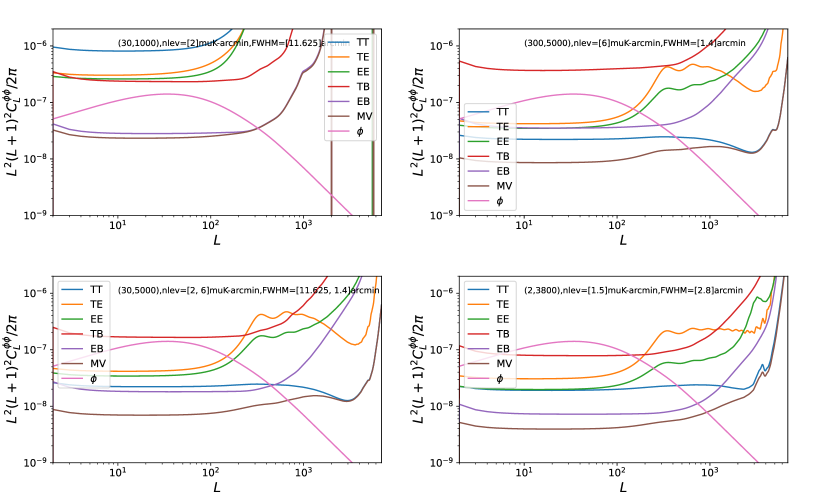
Figure 2: The lensing reconstruction noise power spectrum of the three experiments. The label of each curve represent the two CMB fields used to reconstruct. The noisiest $\phi$ is reconstructed from the gSAT (top-left), and combining it with the gLAT (top-right) leads to a reduction in reconstruction noise (bottom-left). The best performance is from the Satellite (bottom-right).

Next, we perform Wiener-filtering on the $\phi$ maps:

$$\begin{gathered}\phi_{LM}\Rightarrow\frac{C_{\ell}^{\phi\phi}}{C_{\ell}^{\phi\phi}+N_{\ell}^{\phi\phi}}\phi_{LM}.\end{gathered}$$ (41)

4.3 Delensing

Regarding the lensing template method, we proceed by converting the spin-2 fields $Q+iU$ to spin-1 and spin-3 fields, and transform the spin-0 potential field to spin-$-1$ and spin-1 fields using CMBlensplus. It’s important to note that only E-modes are included in the QU fields. Following this conversion, we compute the gradient lensing template according to Eq.(17) and Eq.(18). The resulting QU represents the lensing effect on E-mode, from which the lensing B-mode can be separated using harmonic transformation. We then directly subtract it from the observed B maps to obtain the delensed B maps.

Regarding the Inverse-lensing method, we proceed by estimating the inverse deflection angle $\beta$ from the filtered potential, following Eq.(21) using CMBlensplus. Subsequently, we remap the filtered observed QU maps to obtain the delensed QU maps. These are then subtracted from the observed QU maps to derive the noisy lensing template QU maps. The lensing template B map can be separated through harmonic transformation.

We compute the pseudo-Cl of the delensed B $C_{\ell}^{del}$ and the instrumental noise $N_{\ell}^{BB}$ using the NaMaster code, the delensing fraction is calculated by the ratio of the difference between $C_{\ell}^{del}$ and $N_{\ell}^{BB}$ to the theoretical lensing B-mode power spectrum $C_{\ell}^{lens}$. As for the noise debias, we input the required CMB maps and the potential maps according to Eq.26 and Eq.27 to the same pipeline as described above to simulate all the noise bias terms, their auto- pseudo-Cl (we have checked that all the cross- spectrum are safely negligible) are then also calculated using the NaMaster code. We can further subtract them from the delensed B pseudo-Cl $C_{\ell}^{del}$ before calculating the delensing fraction.

4.4 Results

Figure 3: The lensing template B map and delensed B map of the two delensing methods. The top three plots are from the gradient-order template method, and the bottom three are from the inverse-lensing method. We use the same input lensed B map for comparing the output. One can observe an obvious correlation between the input lensed B (left) and the lensing template B (medium), and the fading in the delensed B (right).

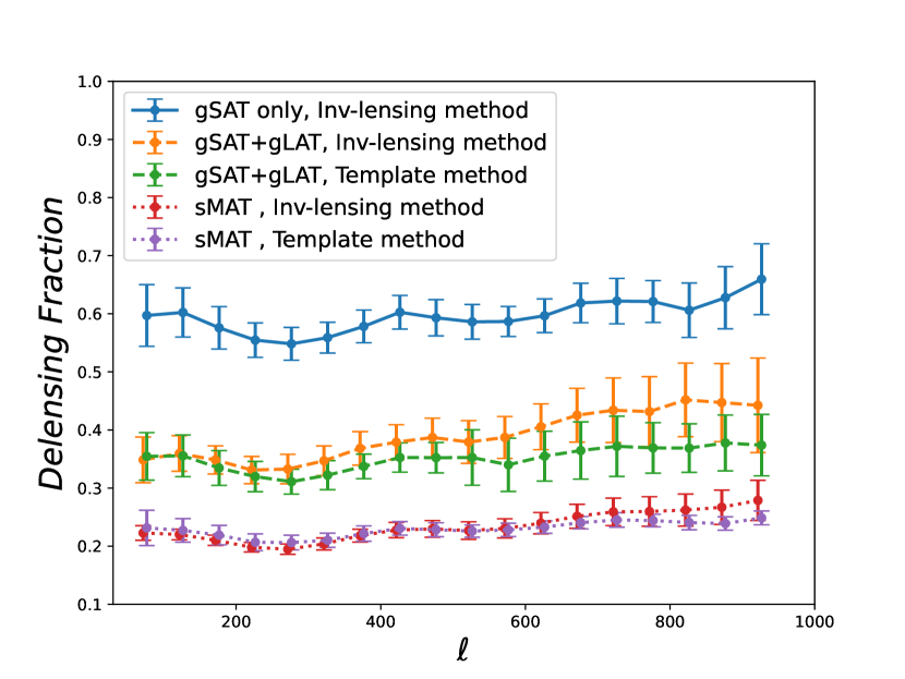
Figure 4: The delensing fraction of the three experiments with two methods. The solid blue shows gSAT delensing performance, the orange and green dashed lines represent the delensing fraction with inverse-lensing method and gradient order template method if we combine gSAT and gLAT. We show the delensing performance of the sMAT with two method separately in red and purple dotted lines.

We plot the delensing fraction in Fig. 4. We observe good consistency between the two methods for both experiments. However, the inverse-lensing method yields slightly higher values compared to the template method, this is due to the noise bias introduced during the delensing procedure. This is evident in Fig. 5, where the removal of the noise power results in perfect consistency between the two methods. This suggests that the biases of lensing residual introduced by the methods themselves are comparable. The primary difference between the two methods lies in the noise spectra during the delensing procedure. For the gradient method, utilizing Eq. (2), we derive $P^{temp}=\nabla P\cdot\nabla\phi$. Consequently,

$$P^{del} =P^{obs}-P^{temp}$$ (42)

$$=P^{len}+P^{noise}-\mathcal{W}^{E}\mathcal{W}^{\phi}\nabla(P^{len}+P^{noise})(\nabla\phi+\nabla\phi^{noise})$$

$$=\left\{P^{len}-\mathcal{W}^{E}\mathcal{W}^{\phi}\nabla P^{len}\nabla\phi\right\}+P^{noise}$$

$$-\left\{\mathcal{W}^{E}\mathcal{W}^{\phi}\nabla P^{noise}(\nabla\phi+\nabla\phi^{noise})+\mathcal{W}^{E}\mathcal{W}^{\phi}\nabla P^{len}\nabla\phi^{noise}\right\},$$

where $P=Q\pm iU$ and this equation corresponds to Eq.(26), as the first brace corresponds to the residual B, and the second brace corresponds to noise biases in Eq.(26).

As for the inverse-lensing method, from Eq.(27) and up to gradient order we have,

$$P^{del} \approx\mathcal{W}^{E}(P^{len}+P^{noise})(n-\mathcal{W}^{\phi}(\nabla\hat{\phi}+\mathcal{O}(\nabla\hat{\phi})^{2}))$$ (43)

$$\approx\mathcal{W}^{E}(P^{len}+P^{noise})(n)$$

$$\quad-\mathcal{W}^{E}\mathcal{W}^{\phi}\nabla(P^{len}+P^{noise})\nabla(\phi+\phi^{noise})$$

$$=\left\{\mathcal{W}^{E}P^{len}-\mathcal{W}^{E}\mathcal{W}^{\phi}\nabla P^{len}\nabla\phi\right\}+\mathcal{W}^{E}P^{noise}$$

$$-\left\{\mathcal{W}^{E}\mathcal{W}^{\phi}\nabla P^{noise}(\nabla\phi+\nabla\phi^{noise})+\mathcal{W}^{P^{E}}\mathcal{W}^{\phi}\nabla P^{len}\nabla\phi^{noise}\right\},$$

Notice that we have neglected high-order terms since the second line, and $\mathcal{W}^{E}=C_{\ell}^{EE}/(C_{\ell}^{EE}+n_{\ell}^{EE})$ in the first term of the third line is close to unity because the E-mode signal is much stronger than its noise. Therefore, up to the gradient order, the delensing noise bias of the two methods is nearly equal. However, in practice, we find that it is the noise bias on small scales arising from the neglected high-order terms in Eq. (43) that causes the inverse-lensing method result to delensing fraction slightly exceed the template method. We thus conclude that the inverse-lensing method is particularly sensitive to noise bias, especially on small scales.

The blue solid line indicates that using 0.8m-gSAT allows for the removal of approximately $40\%$ of the lensing B-modes power. This outcome is expected due to the large full width at half maximum (FWHM), which limits the observation of small-scale CMB polarization. Consequently, a significant reconstruction noise in the lensing potential occurs, degrading the delensing process.

Combining the 0.8m-gSAT with 6m-gLAT further enhances delensing by removing an additional $25\%$ of the lensing B-modes. This combination effectively reduces the FWHM, thereby decreasing the noise in the lensing potential as shown in Fig.2 and improving the signal-to-noise ratio in the observed CMB maps.

Future satellite experiments perform optimally in delensing due to their high signal-to-noise ratio in detecting small-scale features. These experiments can remove approximately $80\%$ of the lensing B-modes using either of the two delensing methods.

4.5 Results on the lensing residual

Comparing to Fig. 4, the lensing residual fractions are greatly reduced by approximately 10% to 20% for the two methods in each experiment. This reduction is consistent with the statement made in Section 2.3, where we discussed that the delensing noise bias contributes to the final delensed B-modes and can be removed in the power spectrum. We observe a high degree of consistency in the fraction of the two methods, as mentioned above. This confirms the theoretical analysis indicating that the lensing template method and the inverse lensing method are almost equal in principle.

Furthermore, as discussed in Section 2.3.3, achieving a smaller bias on $r$ requires flatter fractions. Notably, the lensing residual fractions exhibit a flatter behavior compared to the delensing fraction. Therefore, for future $r$ constraint with delensing, adopting the parameterization described in Eq. 35 and utilizing our method to estimate the delensing noise spectra would be advisable.

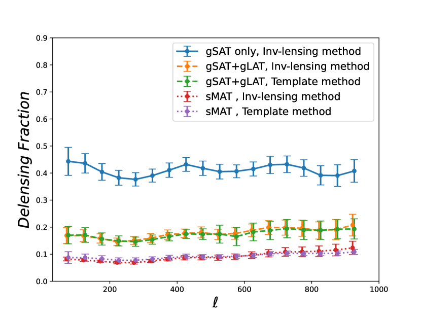
Figure 5: The ratio between lensing residual spectra and lensing spectra of the three experiments with two methods. The solid blue is from gSAT, the orange and green dashed lines are given by the inverse-lensing method and gradient order template method if we combine gSAT and gLAT, and the results of the sMAT with two method separately in red and purple dotted lines.

4.6 Comparison between the methods

In practice, we observe that the gradient order template performs better than the non-perturbative order template, and the inverse-lensing method performs at the same level as the gradient order template.

Firstly, we learn from the detailed calculations presented in Baleato Lizancos et al. (2021) that the gradient order template outperforms the non-perturbative order template due to its ability to cancel the second-order terms when computing the residual B-modes power spectrum. These second-order terms significantly contribute to the delensing fraction, thereby leading to better performance of the gradient order template.

Secondly, we notice that the inverse-lensing method performs comparably to the gradient order template, contrary to the findings in Baleato Lizancos et al. (2021). This discrepancy arises because they made an approximation assuming that $\beta=-\nabla\phi=-\alpha$ when calculating the inverse deflection angle.

$$\begin{gathered}\beta(\hat{n})=-\alpha(\hat{n}+\beta(\hat{n}))=-\alpha(\hat{n})-\nabla\alpha(\hat{n})\cdot\beta(\hat{n})-\dots,\end{gathered}$$ (44)

We can see that neglecting the second-order term $\nabla\alpha(\hat{n})\cdot\beta(\hat{n})$ when using the approximation $\beta$ results in retaining the second-order lensing effect in the remapped field. Consequently, this leads to the persistence of a second term in the residual B-modes power spectrum, thereby deteriorating performance.

However, in our methodology, we employ an iterative approach instead of relying on approximations. This iterative method effectively incorporates the second-order term $\nabla\alpha(\hat{n})\cdot\beta(\hat{n})$ into $\beta$. Consequently, it ensures that the second-order lensing effect is properly accounted for in the remapped field. As a result, the second terms in the residual B-modes power spectrum are canceled out, leading to comparable performance with the gradient order template method. For more details, please refer to Baleato Lizancos et al. (2021).

In terms of implementation efficiency, the non-perturbative template method stands out as the fastest. This is because it only requires using Lenspyx to remap the lensed maps again with $\phi$ map, which is a relatively quick process. The gradient order template method follows as the second fastest. While calculating the gradient of QU maps and potential maps isn’t slow, the E-B correction step can be time-consuming. On the other hand, the inverse-lensing method is the slowest. Although calculating the inverse deflection angle $\beta(\hat{n})$ isn’t slow, remapping the lensed maps with $\beta(\hat{n})$ using CMBlensplus proves to be time-consuming, leading to longer processing times compared to the other two methods.

In conclusion, we recommend considering both the gradient order template and the inverse-lensing method for delensing tasks. The gradient order template is widely used, while the inverse-lensing method offers a more intuitive and straightforward conceptual framework. However, it’s important to note that while both methods can achieve comparable results, the inverse-lensing method typically requires more computational time due to the remapping process. Additionally, under specific conditions, particularly on smaller scales, the delensed maps produced by the inverse-lensing method may exhibit slightly more delensing noise biases.

5 Discussion and Conclusion

In this paper, we demonstrate CMB B-mode delensing through gradient-order and inverse-lensing methods, offering a comprehensive analysis of both the delensing residual delensing originating from the methods themselves and the delensing noise biases stemming from instrumental noise and those from the reconstruction of $\phi$. We investigate the delensing fraction using simulated data obtained from both small-aperture and larger-aperture ground-based telescopes, as well as space missions equipped with medium-aperture instruments.

The results reveal that a ground-based small-aperture CMB polarizing telescope achieves a stand-alone lensing B-mode removal efficiency of 40%. This efficiency increases to 65% when combined with a large-aperture telescope. In contrast, the future satellite experiment achieves an impressive removal efficiency of approximately 80%. Both methods can attain comparable lensing residuals. However, the inverse-lensing method typically demands more computational time due to its remapping process. Additionally, it tends to exhibit larger delensing noise bias on small scales.

We will enhance our delensing pipeline by integrating internal lensing potential reconstruction techniques. Additionally, we plan to combine the lensing potential maps with other $\phi$ tracers, such as the Cosmic Infrared Background, to increase the signal-to-noise ratio of the lensing potential and improve the delensing efficacy. What’s more, we notice that recently the iterative internal delensing method has been performed in Belkner et al. (2023), and we will further compare the performance of the iterative delensing method with the two methods in the future work. Additionally, we will provide a more comprehensive analysis of delensing performance across the three experiments, accounting for foreground emissions and inhomogeneous noise. Subsequently, we will demonstrate the enhancements in constraints on Primordial Gravitational Waves (PGWs) with delensing.

Appendix A Some algorithms of delensing effect

Here we want to highlight an algorithms of delensing effect, which may be useful when separating the components of the delensing output. We first assume we remap a lensed field with a sum of two potential field $\phi=\phi_{1}+\phi_{2}$, and their inverse-lensing angle is $\beta_{1}$ and $\beta_{2}$ respectively. We assume the total inverse-lensing angle $\beta\approx\beta_{1}+\beta_{2}$, we have to admit that this neglects the second order term of $\beta$ (the gradient operation is linear, while the iteration is not), but it seems not a big deal to our final results. Then we can write the delensed field as:

$$X^{de}(n) \approx\tilde{X}(\hat{n}+\beta_{1}+\beta_{2})$$ (45)

$$\approx\tilde{X}(\hat{n})+\nabla\tilde{X}(\hat{n})(\beta_{1}+\beta_{2})+\frac{1}{2}\nabla^{2}\tilde{X}(\hat{n})(\beta_{1}+\beta_{2})^{2}+\mathcal{O}(\beta^{2})$$

$$\approx\left[\tilde{X}^{de}(\hat{n})+\nabla\tilde{X}^{de}(\hat{n})\beta_{1}+\frac{1}{2}\nabla^{2}\tilde{X}^{de}(\hat{n})\beta_{1}^{2}\right]$$

$$+\left[\tilde{X}^{de}(\hat{n})+\nabla\tilde{X}^{de}(\hat{n})\beta_{2}+\frac{1}{2}\nabla^{2}\tilde{X}^{de}(\hat{n})\beta_{2}^{2}\right]+\mathcal{O}(\beta^{2})$$

$$\approx\tilde{X}^{de}(\hat{n}+\beta_{1})+\tilde{X}^{de}(\hat{n}+\beta_{2})-\tilde{X}^{de}(\hat{n})+\mathcal{O}(\beta^{2}).$$

However, if we delens a sum of two lensed field $\tilde{X}=\tilde{X}_{1}+\tilde{X}_{2}$ with one potential, it will be easy finding that this just a linear algorithms, so:

$$X^{de}(n)=X_{1}(\hat{n}+\beta)+X_{2}(\hat{n}+\beta)=X_{1}^{de}(\hat{n})+X_{2}^{de}(\hat{n}).$$ (46)

Above all, we can summary here the delensing algorithms :

$$X\star\left(\phi_{1}+\phi_{2}\right)\approx X\star\phi_{1}+X\star\phi_{2}-X+\mathcal{O}(\beta^{2}),$$ (47)

$$(X_{1}+X_{2})\star\phi=X_{1}\star\phi+X_{2}\star\phi.$$

Here we mean the $\star$ is the delensing operation, and $X$ the CMB field, instrumental noise or the observed CMB field, and $\phi$ the lensing potential or its reconstruction noise.

As for the gradient order template method, we find the lensing template map is straightforward and just obeys a linear algorithms as :

$$\begin{gathered}\nabla[(Q_{1}+Q_{2})\pm i(U_{1}+U_{2})](\hat{n})\nabla[\phi_{1}(\hat{n})+\phi_{2}(\hat{n})]\\ =\nabla[Q_{1}\pm iU_{1}](\hat{n})\nabla[\phi_{1}(\hat{n})]+\nabla[Q_{2}\pm iU_{2}](\hat{n})\nabla[\phi_{2}(\hat{n})]\\ +\nabla[Q_{2}\pm iU_{2}](\hat{n})\nabla[\phi_{1}(\hat{n})]+\nabla[Q_{1}\pm iU_{1}](\hat{n})\nabla[\phi_{2}(\hat{n})].\end{gathered}$$ (48)

Appendix B Wiener filter

B.1 Definition and derivation

The well-known form of Wiener filter is written as:

$$\frac{S}{S+N},$$ (49)

where $S$ represents the power spectrum of signal, and $N$ is the power spectrum of noise.

Here we will derive it from the delensing aspect. We provide two kind of understanding. We will see that the principle of Wiener filter is to minimize the residuals (or called error).

B.1.1 Derivation using gradient template method

We work in flat sky for simplicity. We start from the observed B-modes, which consists of PGWs induced B-modes , lensing induced B-modes and noise

$$B^{obs}(l)=B^{tens}(l)+B^{lens}(l)+B^{noise}(l).$$ (50)

Learning that the lensed B-modes can be written as follows (up to gradient order)

$$B^{lens}(l)=-\int\frac{d^{2}l^{\prime}}{2\pi}sin2(\psi_{l^{\prime}}-\psi_{l})l^{\prime}\cdot(l-l^{\prime})E(l^{\prime})\phi(l-l^{\prime}).$$ (51)

We write the lensing template B-modes by replace E-moeds and $\phi$ above with weighted observed E-modes and $\phi$ respectively as

$$B^{temp}(l)=-\int\frac{d^{2}l^{\prime}}{2\pi} sin2(\psi_{l^{\prime}}-\psi_{l})l^{\prime}\cdot(l-l^{\prime})$$ (52)

$$\times\mathcal{W}_{l^{\prime}}^{E}E^{obs}(l^{\prime})\mathcal{W}_{|l-l^{\prime}|}^{\phi}\phi^{obs}(l-l^{\prime}).$$

Then the delensed B-modes can be written as

$$\begin{gathered}B^{del}(l)=B^{obs}(l)-B^{temp}(l)=B^{tens}(l)+B^{noise}(l)+B^{res}(l),\end{gathered}$$ (53)

where the residual B-modes is

$$\begin{gathered}B^{res}(l)=B^{lens}(l)-B^{temp}(l)=-\int\frac{d^{2}l^{\prime}}{2\pi}sin2(\psi_{l^{\prime}}-\psi_{l})l^{\prime}\cdot(l-l^{\prime})\\ \times\left[E(l^{\prime})\phi(l-l^{\prime})-\mathcal{W}_{l^{\prime}}^{E}E^{obs}(l^{\prime})\mathcal{W}_{|l-l^{\prime}|}^{\phi}\phi^{obs}(l-l^{\prime})\right].\end{gathered}$$ (54)

Then we can write the power spectrum of residual B-modes as

$$C_{l}^{res}\cdot(2\pi)^{2} =\langle B^{res}(l)B^{res*}(l)\rangle$$ (55)

$$=\int\frac{d^{2}l_{1}}{2\pi}\int\frac{d^{2}l_{2}}{2\pi}\sin 2(\psi_{l_{1}}-\psi_{l})\sin 2(\psi_{l_{2}}-\psi_{l})$$

$$\times\left[l_{1}\cdot(l-l_{1})\right]\left[l_{2}\cdot(l-l_{2})\right]$$

$$\times\langle\left[E(l_{1})\phi(l-l_{1})-\mathcal{W}_{l_{1}}^{E}E^{obs}(l_{1})\mathcal{W}_{|l-l_{1}|}^{\phi}\phi^{obs}(l-l_{1})\right]$$

$$\times \left[E^{*}(l_{2})\phi^{*}(l-l_{2})-\mathcal{W}_{l_{2}}^{E}E^{obs*}(l_{2})\mathcal{W}_{|l-l_{2}|}^{\phi}\phi^{obs*}(l-l_{2})\right]\rangle.$$

Using Wick’s theorem and noticing that

$$\langle E(l_{1})E^{*}(l_{2})\rangle=(2\pi)^{2}\delta^{2}(l_{1}-l_{2})C_{l_{1}}^{EE},$$ (56)

$$\langle\phi(L_{1})\phi^{*}(L_{2})\rangle=(2\pi)^{2}\delta^{2}(L_{1}-L_{2})C_{l_{1}}^{\phi\phi},$$

$$\langle E(l_{1})n^{E*}(l_{2})\rangle=0\Rightarrow\langle E(l_{1})E^{obs*}(l_{2})\rangle,$$

$$\langle\phi(L_{1})n^{\phi*}(L_{2})\rangle=0\Rightarrow\langle\phi(L_{1})\phi^{obs*}(L_{2})\rangle,$$

$$\langle E^{obs}(l_{1})E^{obs*}(l_{2})\rangle=(2\pi)^{2}\delta^{2}(l_{1}-l_{2})\left[C_{l_{1}}^{EE}+N_{l_{1}}^{EE}\right],$$

$$\langle\phi^{obs}(L_{1})\phi^{obs*}(L_{2})\rangle=(2\pi)^{2}\delta^{2}(L_{1}-L_{2})\left[C_{L_{1}}^{\phi\phi}+N_{L_{1}}^{\phi\phi}\right],$$

Substituting the above equations into the equation of $C_{l}^{res}$, and questing for the minimum of $C_{l}^{res}$, we can get the Wiener filter as

$$\frac{\partial C_{l}^{res}}{\partial\mathcal{W}_{l_{1}}^{E}\mathcal{W}_{|l-l_{1}|}^{\phi}} =\int\frac{d^{2}l_{1}}{2\pi}g^{2}(l_{1},l)[-C_{l_{1}}^{EE}C_{|l-l_{1}|}^{\phi\phi}$$ (57)

$$+\mathcal{W}_{l_{1}}^{E}\mathcal{W}_{|l-l_{1}|}^{\phi}(C_{l_{1}}^{EE}+N_{l_{1}}^{EE})(C_{|l-l_{1}|}^{\phi\phi}+N_{|l-l_{1}|}^{\phi\phi})]=0,$$

$$\Rightarrow\mathcal{W}_{l_{1}}^{E}\mathcal{W}_{|l-l_{1}|}^{\phi}=\frac{C_{l_{1}}^{EE}}{C_{l_{1}}^{EE}+N_{l_{1}}^{EE}}\cdot\frac{C_{|l-l_{1}|}^{\phi\phi}}{C_{|l-l_{1}|}^{\phi\phi}+N_{|l-l_{1}|}^{\phi\phi}}.$$

Therefore, the lensing template we construct is

$$B^{temp}(l) =-\int\frac{d^{2}l^{\prime}}{2\pi}sin2(\psi_{l^{\prime}}-\psi_{l})l^{\prime}\cdot(l-l^{\prime})\mathcal{W}_{l^{\prime}}^{E}E^{obs}(l^{\prime})$$ (58)

$$\times\mathcal{W}_{|l-l^{\prime}|}^{\phi}\phi^{obs}(l-l^{\prime})$$

$$=-\int\frac{d^{2}l^{\prime}}{2\pi}sin2(\psi_{l^{\prime}}-\psi_{l})l^{\prime}\cdot(l-l^{\prime})$$

$$\times\left[\frac{C_{l_{1}}^{EE}}{C_{l_{1}}^{EE}+N_{l_{1}}^{EE}}E^{obs}(l^{\prime})\right]\left[\frac{C_{|l-l_{1}|}^{\phi\phi}}{C_{|l-l_{1}|}^{\phi\phi}+N_{|l-l_{1}|}^{\phi\phi}}\phi^{obs}(l-l^{\prime})\right].$$

Obviously, this filtered template is a scaled version of the lensed B-modes due to the suppression of Wiener filter on signal.

Notice that if the beam effect is not contained in the noise power spectrum, the Wiener filter should be modified as follows:

$$E^{obs}_{\ell m}=E_{\ell m}b_{\ell}+n^{E}_{\ell m},$$ (59)

$$\Rightarrow\mathcal{W}^{E}_{\ell}E^{obs}_{\ell m}=b_{\ell}\mathcal{W}^{E}_{\ell}\left(E_{\ell m}+n^{E}_{\ell m}/b_{\ell}\right),$$

$$\Rightarrow b_{\ell}\mathcal{W}^{E}_{\ell}=\frac{C_{\ell}^{EE}}{C_{\ell}^{EE}+N_{\ell}^{EE}/b_{\ell}^{2}}\Rightarrow\mathcal{W}^{E}_{\ell}=\frac{1}{b_{\ell}}\frac{C_{\ell}^{EE}}{C_{\ell}^{EE}+N_{\ell}^{EE}/b_{\ell}^{2}},$$

where we just replace $b_{\ell}\mathcal{W}^{E}_{\ell}$ with original $\mathcal{W}^{E}_{\ell}$, and the beam effect is not contained in the noise power spectrum.

B.1.2 Derivation using inverse-lensing method

We try to follow Green et al. (2017) to derive the Wiener filter from another perspective. We refer the reader to this article for its contribution to the understanding of Wiener filter in a more thorough view. Here we only give a brief introduction , more detail calculation can be find there.

For an observed field, different multipoles may have different signal-to-noise ratio, while most of the parts are signal dominated, some part can be corrupted by noise. So, we artificially divide the observed field into two parts, one is signal dominated, the other is noise dominated, with three filter operators $h$ , $\bar{h}$ and $g$. We want the signal dominated part to be remapped to the unlensed CMB, while the noise dominated part to be unchanged. Then the delensed field can be written as (we use temperature field for instance, and can be generalized to QU fields without losing generality)

$$\begin{gathered}T^{d}(\hat{x})=\bar{h}\star T^{obs}(\hat{x})+h\star T^{obs}(\hat{x}-g\star\alpha^{obs}(\hat{x})).\end{gathered}$$ (60)

As for the reason of division, we leave it to the next subsection. This is actually the inverse-lenisng method we introduced before, while there only remap the second part of the observed field which are signal-dominated, and leave the noise-dominated part unchanged. We expect this choice will improve the delensing by improving the input SNR.

We know that lenisng conserves the total power, so we here obey this rule to mimic the lensing effect since inverse-lensing is essentially also a kind of lensing

$$\begin{gathered}\langle T^{d}(0)^{2}\rangle=\langle T^{obs}(0)^{2}\rangle.\end{gathered}$$ (61)

After a short calculation, we can get the relation between $h$ and $\bar{h}$

$$\begin{gathered}\bar{h}_{\ell}=\sqrt{1-h_{\ell}^{2}\left(1-e^{-\frac{\ell^{2}}{2}C_{0}^{obs}(0)}\right)}-h_{\ell}e^{-\frac{\ell^{2}}{4}C_{0}^{obs}(0)}.\end{gathered}$$ (62)

The filter are derived demanding the minimize the variance below (B.7) of Green et al. (2017)

$$\begin{gathered}\langle(T_{\ell}^{d}-\langle T_{\ell}^{d}\rangle_{\phi,\phi^{N}})(T_{-\ell}^{d}-\langle T_{-\ell}^{d}\rangle_{\phi,\phi^{N}})\rangle_{T,\phi,\phi^{N}}.\end{gathered}$$ (63)

An intuition for this choice is that we are demanding that we minimize how much $T^{d}$ varies with each realization of the lensing field and the reconstruction noise. More explicitly, this looks like the variance of the delensed filed.

This actually corresponds to demanding the minimum of residuals, which we define as the difference between the lensed field and the template field. Now we get the delensed field, and the template field can be the difference between the lensed field and the delensed field.

$$\begin{gathered}T^{del}(l)=T^{obs}(l)-T^{temp}(l)=T^{tens}(l)+T^{noise}(l)+T^{res}(l),\end{gathered}$$ (64)

If we first average over the lensing potential and its noise, then $T^{tens}(l)$ and $T^{noise}(l)$ will not change and $(T_{\ell}^{d}-\langle T_{\ell}^{d}\rangle_{\phi,\phi^{N}})$ thus equal to $(T_{\ell}^{res}-\langle T_{\ell}^{res}\rangle_{\phi,\phi^{N}})$, then we average its norm square over all field realizations, we can get the variance of the residual field. So, here we actually still demanding the minimum of residuals, but in a more indirect way.

After some complicated calculation, we get the final output as

$$\begin{gathered}g_{L}=\frac{C_{L}^{\phi\phi}}{C_{L}^{\phi\phi}+N_{L}^{\phi\phi}},\\ h_{\ell}=\frac{\tilde{C}_{\ell}^{T\nabla T}}{C_{\ell}^{obs}}\simeq\frac{\tilde{C}_{\ell}^{TT}}{C_{\ell}^{obs}}.\end{gathered}$$ (65)

B.2 Why do we need Wiener filter in CMB delensing

A brief and mainstream answer is to minimize the residuals by improving the input SNR. Here we give a more detailed explanation.

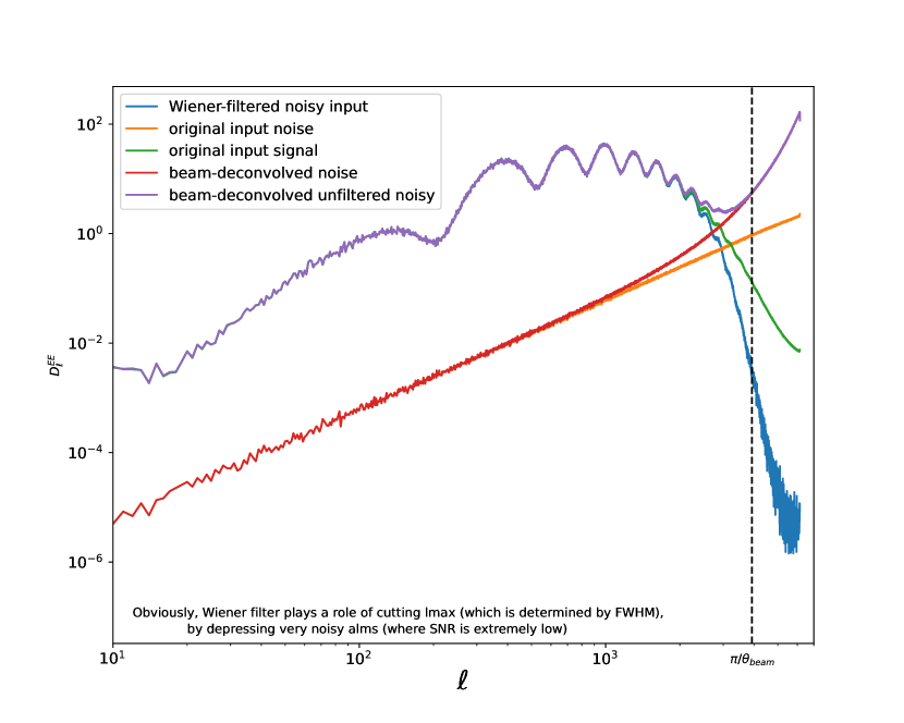
Figure 6: The input signal, noise, signal + noise, and filtered input. Here we show the power spectrum of a deconvolved field before and after Wiener filter One can see that the filtered input become suppressed where SNR is low ($\ell>3000$), and the filtered input is almost the same as the signal where SNR is high.

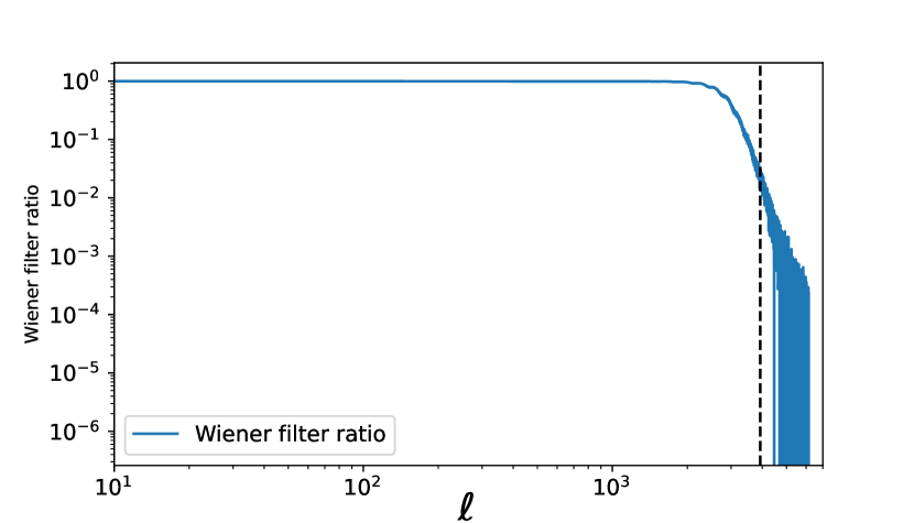
Figure 7: The Wiener filter ratio of the deconvolved field

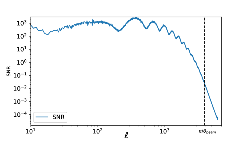
Figure 8: The signal-to-noise ratio of the deconvolved field

We here make a demonstration by simulation. We show the influence on the input data in Fig.6 , Fig.7 and Fig.8. And we artificially supply a peak in the noise power spectrum to emphasise the influence on the delensing output in Fig.9. From Fig.6 , Fig.7 and Fig.8 we can see that the filtered input become suppressed where SNR is low, and the filtered input is almost the same as the signal where SNR is high. The Wiener filter become suppressed after $\ell\approx 2000$, and so does the noisy input (blue). In this way, the Wiener filter divide the noisiest modes from the clean modes, avoiding input the very noisy modes into delensing process.

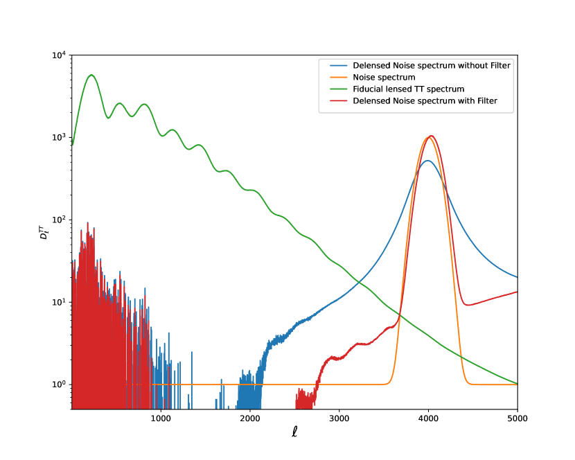
Figure 9: The lensed temperature power spectrum and noise curve in green and orange respectively.The noise power is given a Gaussian packet for illustration. The noise curve after delensing is shown with and without filtering in red and blue respectively. One can see that the filter suppress the expansion of the noise power spectrum during delensing, and the shape of delensed noise curve change a little with a small shift.

We know that lensing will smooth a peak in power spectrum, and when we delensing an observed field which consists of lensed CMB and instrumental noise, we actually lens them all. For the lensed CMB, we expect this lens will recover it to primary CMB. However for the noise, we will smooth its power spectrum due to this lensing. From Fig.9 we see that the unfiltered noise curve exceeds the signal in locations that were signal dominated before delensing, which reduce the SNR of these modes. For a single mode, the noise inside will be remapped to other modes according to the inverse-lensing angle when delensing, causing the noise power to expand especially for an inhomogeneous noise. So the delensed residuals will increase. Thanks to the filtering leaves the noise curves essentially unchanged, which prevents the situation above from happening as much as possible. In a word, filtering improve the delensing by improving the input SNR.

Notice that there is still noise residual after the filtering, which means that the lensing template or the remapped field consists of noise residuals as well. We can perform noise debias on power spectrum by noise-only simulations. Besides, as mentioned before, the filtering will suppress the signal more or less, and we can re-scale the lensing template to compensate for this suppression if necessary, by calculating the transfer function from the signal-only simulations.

References

- Ade et al. (2016a) Ade P. A., et al., 2016a, Phys. Rev. Lett.
- Ade et al. (2016b) Ade P. A., et al., 2016b, Astronomy & Astrophysics, 594, A21
- Ade et al. (2021) Ade P. A., et al., 2021, Physical Review D, 103, 022004
- Aghanim et al. (2020) Aghanim N., et al., 2020, Astronomy & Astrophysics, 641, A8
- Alonso et al. (2023) Alonso D., Sanchez J., Slosar A., Collaboration L. D. E. S., et al., 2023, Astrophysics Source Code Library, pp ascl–2307
- Baleato Lizancos et al. (2021) Baleato Lizancos A., Challinor A., Carron J., 2021, Phys. Rev. D, 103, 023518
- Belkner et al. (2023) Belkner S., Carron J., Legrand L., Umiltà C., Pryke C., Bischoff C., 2023, arXiv preprint arXiv:2310.06729
- Carron (2020) Carron J., 2020, Astrophysics Source Code Library, pp ascl–2010
- Carron et al. (2017a) Carron J., Lewis A., Challinor A., 2017a, JCAP, 05, 035
- Carron et al. (2017b) Carron J., Lewis A., Challinor A., 2017b, Journal of Cosmology and Astroparticle Physics, 2017, 035
- Diego-Palazuelos et al. (2020) Diego-Palazuelos P., Vielva P., Martínez-González E., Barreiro R. B., 2020, JCAP, 11, 058
- Green et al. (2017) Green D., Meyers J., van Engelen A., 2017, JCAP, 12, 005
- Han et al. (2023) Han J., et al., 2023, JCAP, 04, 063
- Kesden et al. (2002) Kesden M., Cooray A., Kamionkowski M., 2002, Physical Review Letters, 89, 011304
- Larsen et al. (2016) Larsen P., Challinor A., Sherwin B. D., Mak D., 2016, Physical Review Letters, 117, 151102
- Lewis & Challinor (2011) Lewis A., Challinor A., 2011, Astrophysics source code library, pp ascl–1102
- Liu et al. (2022) Liu J., et al., 2022, Sci. China Phys. Mech. Astron., 65, 109511
- Lizancos et al. (2021) Lizancos A. B., Challinor A., Carron J., 2021, Journal of Cosmology and Astroparticle Physics, 2021, 016
- Manzotti et al. (2017) Manzotti A., et al., 2017, The Astrophysical Journal, 846, 45
- Namikawa (2021) Namikawa T., 2021, Astrophysics Source Code Library, pp ascl–2104
- Namikawa & Nagata (2014) Namikawa T., Nagata R., 2014, Journal of Cosmology and Astroparticle Physics, 2014, 009
- Namikawa et al. (2012) Namikawa T., Yamauchi D., Taruya A., 2012, Journal of Cosmology and Astroparticle Physics, 2012, 007
- Namikawa et al. (2022) Namikawa T., et al., 2022, Physical Review D, 105, 023511
- Okamoto & Hu (2003) Okamoto T., Hu W., 2003, Phys. Rev. D, 67, 083002
- Sherwin & Schmittfull (2015) Sherwin B. D., Schmittfull M., 2015, Physical Review D, 92, 043005
- Simard et al. (2015) Simard G., Hanson D., Holder G., 2015, The Astrophysical Journal, 807, 166
- Smith et al. (2012) Smith K. M., Hanson D., LoVerde M., Hirata C. M., Zahn O., 2012, Journal of Cosmology and Astroparticle Physics, 2012, 014
- Story et al. (2015) Story K., et al., 2015, The Astrophysical Journal, 810, 50
- Teng et al. (2011) Teng W.-H., Kuo C.-L., Wu J.-H. P., 2011, arXiv preprint arXiv:1102.5729
- Zonca et al. (2019) Zonca A., Singer L., Lenz D., Reinecke M., Rosset C., Hivon E., Gorski K., 2019, Journal of Open Source Software, 4, 1298