The effect of inter-track coupling on H₂O₂ productions

Abstract

Background: Lower production of H₂O₂ in water is a hall-mark of ultra-high dose rate (UHDR) compared to the conventional dose rate (CDR). However, the current computational models based on the predicted yield of H₂O₂ are in opposite of the experimental data.

Purpose: To present a multi-scale formalism to reconcile the theoretical modeling and the experimental observations of H₂O₂ production and provide a mechanism for the suppression of H₂O₂ at FLASH UHDR.

Methods: We construct an analytical model for the rate equation in the production of H₂O₂ from ^.OH-radicals and use it as a guide to propose a hypothetical geometrical inhomogeneity in the configuration of particles in the FLASH-UHDR beams. We perform a series of Monte Carlo (MC) simulations of the track structures for a system of charged particles impinging the medium in the form of clusters and/or bunches.

Results: We demonstrate the interplay of diffusion, reaction rates, and overlaps in track-spacing attribute to a lower yield of H₂O₂ at FLASH-UHDR vs. CDR. This trend is reversed if spacing among the tracks becomes larger than a critical value, with a length scale that is proportional to the diffusion length of ^.OH-radicals modulated by a rate of decay due to recombination with other species, available within a track, and the space among the tracks. The latter is substantial on the suppressing of the H₂O₂ population at FLASH-UHDR relative to CDR. Under these conditions in our MC setup, the reduction of H₂O₂ dose rate effect is attributed mainly to the early time-scale of the e${}^{-}_{\rm aq}$ reaction with ^.OH-radicals and negligible reaction with ^.H.

Conclusions: Based on our analysis of the present work, at FLASH-UHDR, the lower yield in H₂O₂ can be interpreted as a signature of bunching the particles in beams of ionizing radiation. The beams enter the medium in closely packed clusters and form inhomogeneities in the track-structure distribution. Thus the MC simulations based on the assumption of uniformly distributed tracks are unable to explain the experimental data.

I Introduction

Recently an intensive interest in understanding the radio-biological effects of the FLASH ultra-high dose rate (UHDR) radiotherapy has emerged, experimentally and theoretically, due to the observed unique normal tissue sparing of 40 Gy/s and higher [1, 2, 3, 4, 5, 6, 7, 8, 9, 10, 11, 12, 13, 14, 15, 4].

A series of systematic experiments in water have been conducted to compare the yields in H₂O₂ production at two levels of low and high dose rates. Accordingly, the experimental yield at FLASH-UHDR is less than that of conventional dose rates (CDR) [14, 15, 4].

Several research teams have examined the experimental data against the computation of the vastly used reaction rate models for chemical simulation of water radiolysis [16], in addition to the Monte Carlo (MC) computational models [17, 18, 19]. Accordingly, it has turned out that the result of their computational models has predicted contradictory outcomes, i.e., the model calculations have predicted the higher yield of H₂O₂ at FLASH dose rates, compared to CDR.

The present study aims to suggest a theoretical model combined with a Monte Carlo track structure to reconcile the theoretical predictions with the experiments. Following the recent models proposed by the first author [10], in this work, we demonstrate analytically and validate it numerically how the inter-track coupling may be responsible for the lower yield of H₂O₂ at FLASH dose rates.

We parameterize the dose rate by temporal and spatial spacing among the tracks [10, 12, 13]. We show that the yield in the production of H₂O₂ by two ^.OH-radicals increases as track spacing decreases up to a characteristic length where H₂O₂ production saturates and falls to a lower value asymptotically. The specific length is proportional to the effective diffusion length of ^.OH-radicals, that is the mean free path modulated by the scavenging rate.

II Methods and model calculations

Our methods to investigate the effects of inter-track separation on the H₂O₂ yield consist of analytical derivations and testing the predictions by performing a series of experimental Geant4-DNA MC simulations of the track structure. To this end, we used the chemistry and UHDR modules of Geant4-DNA [26, 27, 28, 29, 30].

We calculate the yield in H₂O₂ production based on a non-Poissonian distribution of the deposited dose to demonstrate the scavenging rate of ^.OH-radicals is an increasing function of the tracks compactness. We isolate the production of H₂O₂ by ^.OH-radicals from all other possible chemical reactions, including the recombination of ^.OH-radicals with ^.H and e${}^{-}_{\rm aq}$. In the first part, we take advantage of this simplification and reduce the rate equations to a single non-linear differential equation. In MC, we, however, use the entire rate equations available in the chemistry and UHDR modules of Geant4-DNA.

II.1 Reaction rate equations of a system of many tracks - a Markov chain

Let us consider at time $t$, after radiation, a large number of reactive species (RS), e.g., ^.OH-radicals, ^.H-radicals, $e^{-}_{\rm aq}$, $\cdots$, have been created. They move out of the center of creation randomly, i.e., by boosted thermal diffusion, thermal spikes, shock waves, etc. Once they meet each other within a certain distance, in spatial proximity to each other, they react chemically and form either metastable and short-life time transient complexes of $n$-clusters or stable non-reactive species (NRS or larger compounds), such as H₂O₂ with $n=2$. We call these complexes, NRS, because of their larger mass and lower mobility compared to RS to reach out to bio-molecules and form any types of damage [10].

For the simplicity in modeling, we focus on the dynamics of ^.OH-radicals. The following rate equation, derived from a stochastic Markov chain Master equation, governs the reaction rate of $n$-^.OH-radicals

$$\frac{d\overline{n}(t)}{dt} = \mu\dot{z}-\gamma_{1}\overline{n}-\frac{\gamma_{2}}{2!}\overline{n(n-1)}-\frac{\gamma_{3}}{3!}\overline{n(n-1)(n-2)}$$ (1)

$$- ...-\frac{\gamma_{N}}{N!}\overline{n(n-1)(n-2)...(n-N)}.$$

The first term describes the rate of energy deposition by charged particles. $\mu,\gamma_{1}.\gamma_{2},\cdots$ are reaction rate constants. Their values depend on the spatial and temporal distribution of the tracks, and therefore the dose rate, $\dot{z}$, where $z=\varepsilon/m$ is the specific energy (energy divided by mass) or the deposited dose. Here $\varepsilon$ is the energy, deposited in mass $m$. The second term, linear in $\overline{n}$, describes the scavenging or decay rate of ^.OH-radicals. The over-line is the statistical averaging. The third term describes the formation of a cluster of two out of $n$ ^.OH-radicals. Similarly, the rest describe clustering of three, four, …, and $N$ ^.OH-radicals. The factors $2!,3!,\cdots,N!$ accounts for the combinatorial factors of clustering $N$ objects out $n$-identical objects. Out of these clusters, $\overline{n(n-1)}/2$ gives the population of created H₂O₂ out of $n$ ^.OH-radicals.

The statistical averaging over different moments of the clusters, $\overline{n(n-1)(n-2)...(n-N)}$, can be performed by integrating over a compound Poisson or Neyman’s distribution of type A that governs the probability distribution of deposition dose [22,23,24]

$$Q_{n}(\theta,\Delta)=\sum_{\nu=0}^{\infty}P_{\nu}(\theta)P_{n}(\nu\Delta).$$ (2)

Here $\nu$ is the number of tracks passing through the volume of interest. $\theta$ is proportional to the average number of tracks that give the mean dose. For a given dose, the number of tracks, $\nu$, is a given number, independent of the dose rate. $n$ is the number of collisions that lead to the creation of ^.OH-radicals in a single track out of $M$ initial ionization and molecular excitations leading to the creation of all RS, thus $\Delta$ is a number proportional to the average number of all RS generated in a single track. Here a track and event are interchangeable. Note that $M>n$. Thus $Q_{n}(\theta,\Delta)$ is the reduced density matrix, in a sense that all other RS degrees of freedom (^.H-radicals, $e^{-}_{\rm aq}$, $\cdots$) have been traced/integrated out, $Q_{n}={\rm Tr}_{M}Q_{M}$. Thus $\overline{n}=\sum_{n=0}^{\infty}nQ_{n}(\theta,\Delta)=\theta\Delta$. Similarly, $\overline{n(n-1)}=(\theta^{2}+\theta)\Delta^{2}$, $\overline{n(n-1)(n-2)}=(\theta^{3}+2\theta^{2}+\theta)\Delta^{3}$, $\overline{n(n-1)(n-2)(n-3)}=(\theta^{4}+6\theta^{3}+7\theta^{2}+\theta)\Delta^{4}$, $\cdots$.

After a tedious but straightforward algebra, the rate equation for $\theta$ can be derived

$$\frac{d\theta(t)}{dt} = \mu z\dot{\theta}-(\gamma_{1}+\frac{\gamma_{2}}{2!}\Delta+\frac{\gamma_{3}}{3!}\Delta^{2}+\frac{\gamma_{4}}{4!}\Delta^{3}+\cdots)\theta$$ (3)

$$- (\frac{\gamma_{2}}{2!}\Delta+2\frac{\gamma_{3}}{3!}\Delta^{2}+7\frac{\gamma_{4}}{4!}\Delta^{3}+\cdots)\theta^{2}$$

$$- (\frac{\gamma_{3}}{3!}\Delta^{2}+6\frac{\gamma_{4}}{4!}\Delta^{3}+\cdots)\theta^{3}$$

$$- (\frac{\gamma_{4}}{4!}\Delta^{3}+\cdots)\theta^{4}-\dots$$

Note that the dose rates is equivalent to a change in the number of tracks per unit of time, $\dot{z}=z\dot{\theta}\Delta$ where $z$ is the specific energy (dose) per track. We factorized $\Delta$ which is a variable dependent on the track correlations, to account for the chemical effectiveness of a single track, that in turn, is a function of inter-track separation. Hence the rate equation can only be expressed in terms of dynamical variable $\theta$ with no time dependence on $\Delta$.

Truncating the series in the rate equation beyond the quartic terms in $\theta$ gives

$$\frac{d\theta(t)}{dt} = \mu z\dot{\theta}-\lambda_{\rm eff}(\Delta)\theta-\gamma_{\rm eff}(\Delta)\theta^{2}-\eta_{\rm eff}(\Delta)\theta^{3}-{\cal O}(\theta^{4}),$$

where

$$\lambda_{\rm eff}(\Delta)=\gamma_{1}+\frac{\gamma_{2}}{2!}\Delta+\frac{\gamma_{3}}{3!}\Delta^{2}+\frac{\gamma_{4}}{4!}\Delta^{3}+\cdots$$ (5)

and

$$\gamma_{\rm eff}(\Delta)=\frac{\gamma_{2}}{2!}+2\frac{\gamma_{3}}{3!}\Delta+7\frac{\gamma_{4}}{4!}\Delta^{2}+\cdots$$ (6)

are the polynomials of $\Delta$. The same for $\eta_{\rm eff}(\Delta)$.

In these equations, the parameter $\Delta$ that has been introduced in the energy deposition distribution function, corrects the scavenging rates of RS due to the inter-track correlation of RS, as $\Delta$ depends on the inter-track distances, hence its value depends on the dose rate and the track distributions at a given dose rate. Note that for a given dose rate, and given the inter-track separation, $\Delta$ is a constant of time. We hypothesize under a variation of the dose rate, e.g., from CDR to FLASH-UHDR, the local compactness of RS changes so the numerical values of $\Delta$. It might be useful to recall a close analogy for $\Delta$ with the change of charged particles LET as a function of depth in a medium.

To investigate further the connection between $\Delta$ and track-spacing, we start from the relation $\Delta=\mu z_{D}$ where $z_{D}=(\overline{z^{2}}-\overline{z}^{2})/\overline{z}$ is the renormalized fluctuations of $z$ (for the derivation, see Ref. [24]). Let us consider two tracks with labels 1 and 2 with specific energies $z_{1}$ and $z_{2}$. The total specific energy is given by $z=z_{1}+z_{2}$. Thus $\overline{z}=\overline{z_{1}}+\overline{z_{2}}$. Because the tracks originated from a beam of identical particles, and $z=\varepsilon/m$ where $\varepsilon$ and $m$ are the energy deposition and mass of the medium, we consider the same mass in the denominator of both $z_{1}$ and $z_{2}$, i.e., $m_{1}=m_{2}$. For two tracks with non-zero correlation and overlap (close to each other), $\overline{z_{1}z_{2}}\neq\overline{z_{1}}~{}\overline{z_{2}}$ and

$$z_{D}=\frac{(\overline{z^{2}_{1}}-\overline{z_{1}}^{2})+(\overline{z^{2}_{2}}-\overline{z_{2}}^{2})+2(\overline{z_{1}z_{2}}-\overline{z_{1}}~{}\overline{z_{2}})}{\overline{z_{1}}+\overline{z_{2}}}$$ (7)

Therefore

$$\Delta = \mu z_{D}=\mu\frac{\overline{z_{1}}\Delta_{1}+\overline{z_{2}}\Delta_{2}+2(\overline{z_{1}z_{2}}-\overline{z_{1}}~{}\overline{z_{2}})}{\overline{z_{1}}+\overline{z_{2}}}$$ (8)

$$= \frac{\Delta_{1}+\Delta_{2}}{2}+2\mu\frac{(\overline{z_{1}z_{2}}-\overline{z_{1}}~{}\overline{z_{2}})}{\overline{z_{1}}+\overline{z_{2}}}$$

$$= \frac{\Delta_{1}+\Delta_{2}}{2}+2\mu\frac{{\rm cov}(z_{1},z_{2})}{\overline{z_{1}}+\overline{z_{2}}}$$

where we used $\overline{z_{1}}=\overline{z_{2}}$ for the first term in RHS. By definition, the covariance of two random variables is given by cov$(z_{1},z_{2})=\langle(z_{1}-\langle z_{1}\rangle)(z_{2}-\langle z_{2}\rangle)\rangle=(\overline{z_{1}z_{2}}-\overline{z_{1}}~{}\overline{z_{2}})$. In a special case of two independent $z_{1}$ and $z_{2}$, the covariance will be identical to zero. Thus, the mean ^.OH-radicals population is the algebraic mean of the ^.OH-radicals populations of two tracks, $\Delta=(\Delta_{1}+\Delta_{2})/2$. The factor of 2 in the denominator is the number of tracks, which has automatically appeared. It guarantees $\Delta$ to be a track-averaged parameter, i.e., total ^.OH-radicals divided by the number of tracks. In another extreme limit of two identical tracks, 1 and 2 (with a coincidental source location), $\Delta_{1}=\Delta_{2}$, and $\Delta=\Delta_{1}+\Delta_{2}$. In this situation, two tracks are the constituent of a single track of a fictitious composite particle with double the charge (neglecting the Coulomb repulsion between two particles), hence there is no division by a factor of two. Thus $(\Delta_{1}+\Delta_{2})/2\leq\Delta\leq\Delta_{1}+\Delta_{2}$, within an interval of two extreme configurations of independent and infinitely high correlated tracks. The latter may be realized in an idealistic and hypothetically infinitely high dose rate from a single source point.

From here one can extract formally a two-point correlation function

$${\rm corr}(z_{1},z_{2})=\frac{{\rm cov}(z_{1},z_{2})}{\sigma_{z_{1}}\sigma_{z_{2}}},$$ (9)

where

$$2\mu\frac{{\rm cov}(z_{1},z_{2})}{\overline{z_{1}}+\overline{z_{2}}}=\Delta-\frac{\Delta_{1}+\Delta_{2}}{2}\geq 0.$$ (10)

Here $\sigma_{z_{1}}$ and $\sigma_{z_{2}}$ are the standard deviations of $z_{1}$ and $z_{2}$. Eq. (10) leads us to renormalize $\Delta$ and replace it in the rate Eqs. (5) and (6). Formally, $\Delta\rightarrow\tilde{\Delta}=\Delta-\overline{\Delta}$ where $\overline{\Delta}$ is averaging over geometrical distribution of the tracks. Clearly, $\tilde{\Delta}\geq 0$. For the independent tracks, with zero overlaps, $\tilde{\Delta}=0$. Thus $\tilde{\Delta}$ is an increasing function of the overlap among the tracks. Because $\tilde{\Delta}$ is a positive number and starts from zero (and not from a finite non-zero value), it is more convenient we reformulate our systems of equations, by replacing $\tilde{\Delta}$ for $\Delta$, starting from Eq. (2). Note that the difference between $\tilde{\Delta}$ and $\Delta$ is just a shift by a constant.

II.2 H₂O₂ yield

To calculate the rate of ^.OH-radicals and conversion to H₂O₂, we multiply Eq. (3) by $\tilde{\Delta}$ and obtain the following non-linear equation for $\overline{n}$

$$\frac{d\overline{n}(t)}{dt} = \mu\dot{z}(t)-\lambda\overline{n}-\gamma\overline{n}^{2}-\eta\overline{n}^{3}.$$ (11)

where $\lambda$, $\gamma$, and $\eta$ are polynomials of $\tilde{\Delta}$. In Eq. (11) $\overline{n}^{2}$ and $\overline{n}^{3}=\overline{n}\times\overline{n}^{2}$ represent the population of H₂O₂ and ^.OH-radicals coupling with H₂O₂, respectively. For ease of notation, we removed the subscript, eff, from $\lambda$, $\gamma$, and $\eta$.

For a constant dose rate, Eq. (11) is integrable analytically. For a non-constant dose rate but constant dose, we split this equation into linear ($\overline{n}_{0}$) and non-linear ($\overline{n}_{1}$) terms. We calculate the solution of the linear equation using retarded Green’s function method in which $\overline{n}(t)$ can be expressed in terms of an integral equation and a functional of $\dot{z}(t)$

$$\overline{n}_{0}[\dot{z}(t)]=\mu\int_{-\infty}^{t}dt^{\prime}e^{-\lambda(t-t^{\prime})}\dot{z}(t^{\prime}),$$ (12)

the linear term in $z$. The population yield of H₂O₂ can be calculated by

$$Y_{0}[\dot{z}(t)]=\int_{-\infty}^{t}dt^{\prime}\overline{n}_{0}^{2}(t^{\prime})=\frac{\mu^{2}}{2\lambda}G[\dot{z}(t)]z^{2},$$ (13)

where

$$G[\dot{z}(t)]=\frac{2}{z^{2}}\int_{-\infty}^{\infty}dt\dot{z}(t)\int_{-\infty}^{t}dt^{\prime}e^{-\lambda(t-t^{\prime})}\dot{z}(t^{\prime}).$$ (14)

is the dose-protraction factor (see for example [25]). Eqs. (12) and (13) constitute a linear-quadratic model for ^.OH-radicals pairing or H₂O₂ formation. Eq. (14) presents a cross-contribution from a two-track process that a pair of ^.OH-radicals (created from two individual tracks) yield in the formation of a single H₂O₂. Note that because in this model $\lambda$ is a polynomial of $\Delta$ which itself an inter-track dependent parameter, that in turn may be affected under a change in dose and dose rate, $Y_{0}$, the population of H₂O₂ may not scale like $z^{2}$. It may show some deviations from a quadratic power law in dose (we have seen it in our MC).

The contributions from the non-linear solutions can be calculated perturbatively in terms of a series of $\overline{n}_{0}$. Considering only contribution from $\overline{n}_{0}$, in Sec. III.1, we numerically calculate the dependence of $Y_{0}$ on the dose rates subjected to a constant dose constraint.

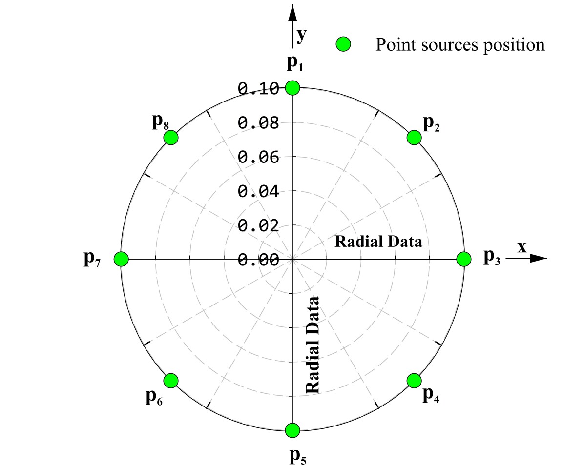
Figure 1: Schematic geometry of source of eight protons (green dots) on an $xy$ planar.

II.3 Monte Carlo simulation

To verify our analytical derivation for the population yield of ^.OH-radicals and H₂O₂, we perform a series of computational experiments by running chemical and UHDR modules of Geant4-DNA MC simulation of the track structure. Many low-energy protons were initialized to impinge a cube-shaped target volume made of water with 19% oxygen content. The physics modules G4EmDNAPhysics (option 2) was used to simulate the physical interactions of the protons with the target. The EmDNAChemistry constructors are used to perform step-by-step production, diffusion, and chemical reactions of the resulting species through the end of the chemical stage, from 1 ps to 1 ms. The thorough spectrum of species and their reactions included in the Geant4-DNA chemistry module were used in the simulation, however, only $\ce{{}^{.}OH}$ and H₂O₂ populations as a function of time were selected for the analysis of the current study. We postpone to submit our entire analysis to our forthcoming publications.

The particle source was modified into a circular $xy$-plane which was located across one side of the water phantom at $z=-16$ nm. The phantom was located at $z=0$. The range of proton energies was chosen up to 1 MeV. Fig. 1 shows the schematic geometry of the protons at the source. The phantom is a homogeneous cube of water with dimensions of 3.2 × 3.2 × 3.2 $\mu$m³. A smaller cube was considered with dimensions of 1.6 × 1.6 × 1.6 $\mu$m³ to score chemical species.

As shown in Fig. 1, each MC simulation consists of mono-energetic protons located on a ring with a specific radius. The protons were ejected along the z-axis toward the water phantom. We keep a fixed radius of the ring in a given simulation and score $\ce{{}^{.}OH}$ and H₂O₂ in water. After performing a series of simulations we plot the population of $\ce{{}^{.}OH}$ and H₂O₂ vs. time and radius of the ring.

This series of simulations must be considered a computational experiment to verify our analytical predictions, resembling hypothetically the inter-track correlations of the dose rate, and examining the influence of the charged particle separation on the chemical end point of this study which is the production of the H₂O₂.

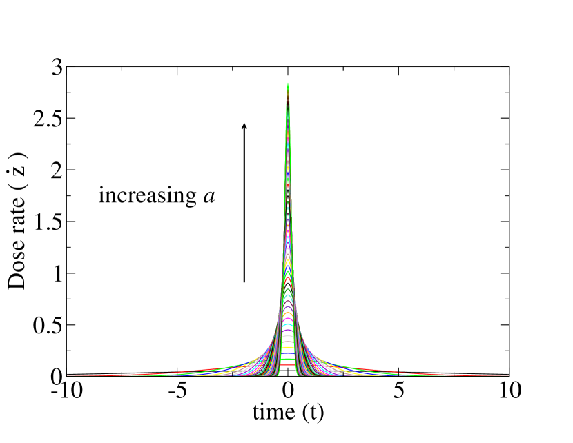
Figure 2: Series of (a) dose rates, and (b) the accumulated ^.OH-radicals, $n_{0}(t)$ as a function of time. $a$ is a parameter that controls the dose rate. The higher $a$, the higher the dose rate subjected to constant dose. All areas under the dose rate curves in (a) are constant and equal to a given deposited dose.

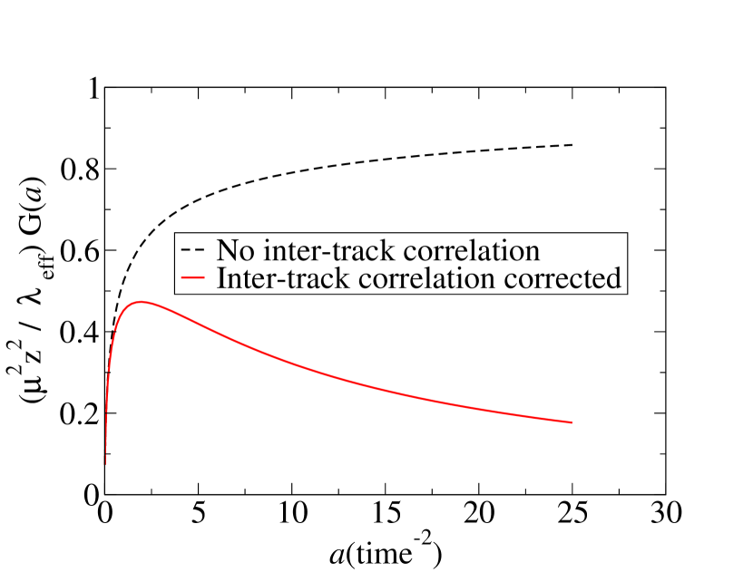
Figure 3: The yield in ^.OH-radicals calculated by Eq.(13). The black dashed lines and the red bold line show the result of the calculation without and with inter-track correlations. They are representative classes of solutions in the Poissonian and non-Poissonian models, respectively.

III Results

III.1 Continuous varying dose rate - analytical model

We illustrate the results from our analytical model for the dose rate, parameterized in a Gaussian function

$$\dot{z}(t)=z\sqrt{\frac{a}{\pi}}e^{-at^{2}}.$$ (15)

subjected to a constant dose constraint, $z=\int_{-\infty}^{\infty}dt\dot{z}(t)=$ const. As shown in Fig. 2, we simulate an increase in the dose rate by increasing the parameter, $a$, continuously and calculate the yield in H₂O₂ as a function of dose rate, as shown in Fig. 3.

In the limit of $a\rightarrow\infty$, $\sqrt{a/\pi}e^{-at^{2}}$ becomes highly sharp around $t=0$. The dose rate becomes singular but integrable, $\sqrt{a/\pi}e^{-at^{2}}\rightarrow\delta(t)$. In this limit, $G[\dot{z}(t)]=1$, thus

$$Y_{0}[\dot{z}(t)]=\frac{\gamma}{2\lambda}z^{2}.$$ (16)

For a finite $a$

$$n_{0}(t)=\mu z\sqrt{\frac{a}{\pi}}e^{-\lambda t}\int_{-\infty}^{\infty}dt^{\prime}e^{\lambda t^{\prime}}e^{-at^{\prime 2}}\theta(t-t^{\prime}),$$ (17)

can be calculated numerically by integration over time.

Fig. 3 shows the dependence of the H₂O₂ on $a$, which is an increasing variable proportional to the dose rate, in the Gaussian model of $\dot{z}$, given by Eq. (15). Thus in Fig. 3, the positive direction of the horizontal axis is the direction of the increase in dose rate. Here the population of H₂O₂, has been normalized to one (the $y$-axis), for a give $a$. Hence, the $y$-axis in Fig. 3 may represent the probability in pairing ^.OH-radicals and forming H₂O₂ as a function of dose rate.

The black dashed curve in Fig. 3 corresponds to a model with no inter-track correlation, e.g., $\tilde{\Delta}=0$ where $\Delta=\overline{\Delta}$. It shows a monotonic increase in the H₂O₂ yield as an increasing function of the dose rate. It resembles one of the results of MC calculation recently presented in [19] (see, e.g., their Fig. 4).

The red solid line corresponds to a model with inter-track correlation, $\Delta$, where $\lambda_{\rm eff}$ is a polynomial in $\Delta$ as given by Eq. (5). In this model, the overall H₂O₂ population reaches a maximum at an optimal value of $a$. Beyond that, it drops continuously and saturates asymptotically to a value at high dose rates, below a value corresponding to lower dose rates.

Note that conceptually the current model is interchangeable with a similar model that describes the formation of DNA double-strand breaks by paring of single-strand breaks and the dependence of the radio-biological effects on $\Delta$ from a single track, proportional to LET [24]. This similarity offers a common characteristic between the high LET and UHDR, by a single parameter, $\Delta$.

In the following section, we perform a series of MC simulations to check these ideas as sketched in Fig 3.

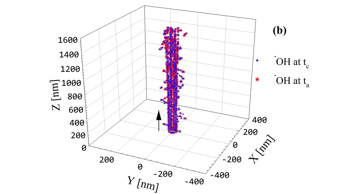
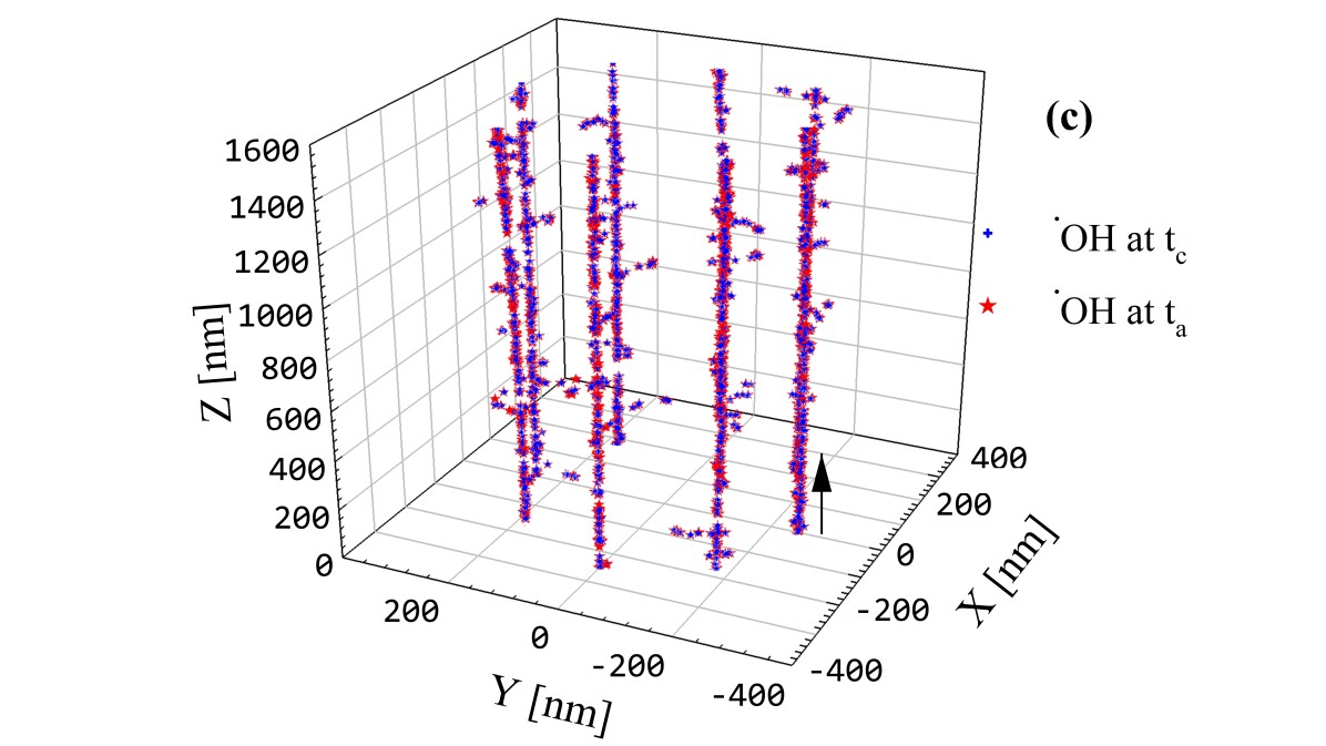
Figure 4: A sample of segments of eight proton tracks in a 1.6 µm length water cube (in $z$-direction), initiated from eight source points located on the planar rings with different radii. The energy of the protons at the point of entrance is 1 MeV. The blue dots show the location of ^.OH-radicals at the creation time t_c. The red dots are the location of $\ce{{}^{.}OH}$ after the diffusion and recombination to H₂O₂ at the annihilation time t_a, where a pair of $\ce{{}^{.}OH}$ within a certain radius, regardless to their relative orientation and magnetic polarization, combine and score a single H₂O₂.

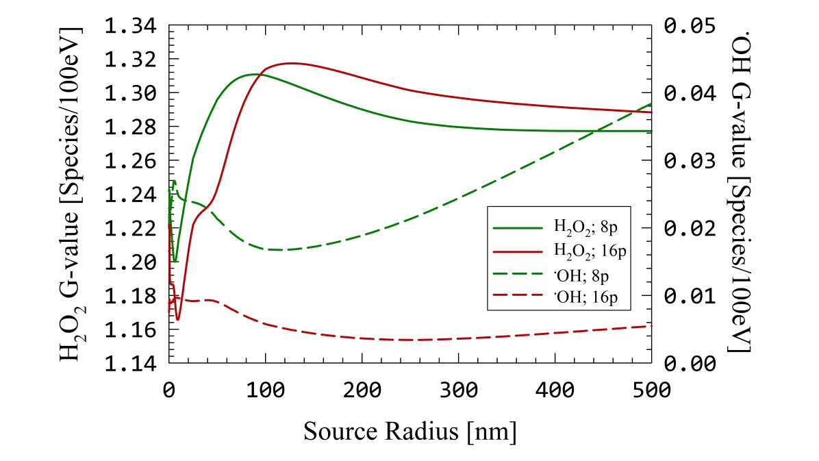
Figure 5: Changes in G-value vs. the source radius of the rings were calculated for eight (green lines) and sixteen (red lines) protons with an initial energy of 1 MeV per proton in a 1.6 mm long cube. Yield in H₂O₂ production (solid lines) and $\ce{{}^{.}OH}$ (dashed lines) are shown at $t=1$ms. An increase in the H₂O₂ yield as a function of inter-track distance is an indication of the higher probabilities in $\ce{{}^{.}OH}$ pairing. At a large ring radius, comparable with the diffusion length of $\ce{{}^{.}OH}$-radicals, the intra-track dominates the inter-track, and H₂O₂ production falls off gradually, a similar effect is shown in Fig. 3.

III.2 Monte Carlo

We employed MC simulations to investigate the effect of inter-track interaction on G-value. Protons with 1 MeV initial energy were ejected from a ring-shaped source. A series of ring radii, $r$, were used to fine-tune the interaction among the tracks continuously. To have full control of the inter-track coupling, we located equally spaced protons on a series of rings with different radii. Thus, an increase in the ring radius, $r$, is assumed to mimic a decrease in the dose rate with higher inter-track spacing.

Fig. 4 shows the particle tracks with source radii of $r=0.5$ nm (a), $r=25$ nm (b), and $r=250$ nm (c). The largest radius demonstrates independent proton tracks, whereas the smallest one corresponds to highly correlated tracks. In this figure, we assume the direction of the dose rate is from bottom to top, hence Fig. 4 (a) and (c) correspond to the highest and the lowest inter-track correlations.

Fig. 5 shows the yield in production and consumption of H₂O₂ and $\ce{{}^{.}OH}$-radicals stemming from eight (green lines) and sixteen (red) protons, respectively. According to our convention, the direction of the dose rate is in the reverse direction of the $x$-axis. We ran these MC simulations up to 1 ms with time steps of 1 ps, a one-million time-step simulation for each ring. Within 1 ms, at a time of annihilation, $t_{a}$, any pair of $\ce{{}^{.}OH}$-radicals fell within a spherical distance smaller than the radius of 0.22 nm, were terminated and scored as a single production of H₂O₂.

The maximum yield in H₂O₂ at a characteristic ring size of $r^{*}$ in Fig. 5 is the hallmark of these simulations. It coincides with a minimum in the population of $\ce{{}^{.}OH}$-radicals.

Below $r^{*}$, on the side of high dose rates, a rise in H₂O₂ is seen as an increasing (decreasing) function of $r$ (dose rate), where the configuration of the tracks resembles the reported experimental data that the H₂O₂ production at FLASH-UHDR is lower than CDR. We, therefore, correlate the experimental data on the yield of H₂O₂ at FLASH-UHDR with the strong inter-track coupling and the entrance of particles in closely space-packed bunches. This explains why track structure calculations based on the uniformly spaced distribution of the tracks end up with a contradictory prediction.

As seen in Fig. 5, above $r^{*}$, the trend in H₂O₂ production reverses. In this limit, the tracks are highly separated, and the prediction of the MC simulation gives a wrong answer to the experimental observations as frequently reported in the literature.

It is also noteworthy that by increasing the number of proton tracks from 8 and 16, we double the dose but the H₂O₂ population doesn’t increase by a factor of 4 as we expected from Eqs. (13) and (14) assuming constant $\lambda$. Our calculation shows that $N_{H2O2}(p=16)/N_{H2O2}(p=8)$ deviates from the quadratic power law in dose as a function of separation among the tracks and the ring-source radius.

A very simplistic calculation of the diffusion length, assuming a diluted gas of $\ce{{}^{.}OH}$-radicals may give a ballpark for $r^{*}$ values. Using the diffusion constant of $\ce{{}^{.}OH}$-radicals given in Geant4-DNA, $D_{f}=2.2\times 10^{-9}$ m²/s, we can calculate the diffusion length using Einstein relation, $\ell=\sqrt{2D_{f}t}$. Taking our maximum simulation time, $t=1$ms, we find $\ell\approx 2100$ nm. Comparing with $r^{*}\approx 100$ nm in Fig. 5, it is clear that $\ell$ is one order of magnitude larger than $r^{*}$. This is due to high reaction rate in $\ce{{}^{.}OH}$-pairing to form H₂O₂, in the rate equation, Eq.(11). In Geant4-DNA, $\gamma=0.55\times 10^{7}$ m³/(mole$\cdot$s). Note that $\gamma$ is the rate of conversion of a pair of $\ce{{}^{.}OH}$-radicals to H₂O₂. In Eq.(11), there is another reaction rate, $\lambda$, that describes conversion of $\ce{{}^{.}OH}$-radicals to all other products (except H₂O₂). In this context, we call $\lambda$, the scavenging rate of $\ce{{}^{.}OH}$-radicals. Using the reaction rates table in Geant4-DNA, $\lambda$ can be calculated by the algebraic sum of all reaction rates (except H₂O₂).

Combining the scavenging rate in the $\ce{{}^{.}OH}$-radicals diffusion equation gives

$$\overline{n}_{0}(\vec{r},t)=\frac{\overline{n}_{0}(\vec{r}=t=0)}{4\pi D_{f}t}\exp\left(-\frac{r^{2}}{4D_{f}t}-\lambda t\right).$$ (18)

From this equation, we may justify why the production of H₂O₂ reaches a maximum at a length scale much lower than the mean free path, $r^{*}<<\ell$. It is simply because of scavenging of $\ce{{}^{.}OH}$-radicals by other species originating from all tracks in the neighborhood, both intra- and inter-track scavenging events. Diffusion is in reverse proportion to RS spatial density, i.e., the denser the volume populated by RS, the slower the diffusion. This is the effect of molecular crowding introduced in our recent publications [10, 12]. On the other hand, the inclusion of thermal spikes boosts dramatically the diffusion constant, however, many of $\ce{{}^{.}OH}$-radicals may still be blocked by molecular crowding in the shock-wave wall of the thermal spikes. Regardless of these details, it must be clear from Fig. 5, that a change in the distance between the particle tracks leads to a change in the G-value for $\ce{{}^{.}OH}$ and H₂O₂ species.

As pointed out, we may expect a significant increase in $r^{*}$ if the effects of thermal spikes, calculated and reported in our recent publications [31] were included in the diffusion constant of chemical species in MC.

For the radial distances less than 100 nm, in the current model and depicted in Fig. 5, the G-value for H₂O₂ shows a decreasing function of the track spacing. Conversely, $\ce{{}^{.}OH}$ shows an increasing trend. The H₂O₂ yield goes up steeply until it reaches a maximum. Beyond that track spacing, it decreases and saturates asymptotically. These changes have the reverse trend on $\ce{{}^{.}OH}$. These ascending and descending trends demonstrate the role of inter-track recombination.

The results of our calculation for the H₂O₂ G-value resemble similar behavior from a circular source with a radius of 1 nm, calculated using TOPAS n-Bio by Derksen et al. [19], (see, Fig. 5 in that reference). Interestingly, with an increase in radius to 100 nm, the maximum in the G-value for H₂O₂ disappears [19] which is, indeed, in agreement with our no-correlation model, shown by black dashed lines in Fig. 3.

IV Discussion and conclusion

The relevance of inter-track interaction has recently been examined in [18] by MC simulation of interacting proton tracks, where no significant changes in ^.OH-radicals or H₂O₂ yields was found at clinically relevant doses. This claim is also supported by other simplistic geometric track overlap models.

These computational results stand in contrast with the experimental evidence of [14] who measured lower H₂O₂ yields at UHDR compared to CDR. Furthermore, [4] and [15] observed a similar decrease in H₂O₂ yields at UHDR with electrons. This discrepancy, as well as the observation that MC simulations tend to measure an increase in H₂O₂ yields as dose rate increases as opposed to the experimentally measured decrease in H₂O₂ yields, suggests that the current model calculations and MC simulations do not provide an adequate representation of the interdependent chemical reactions occurring in the irradiation of oxygenated water.

In this work, we developed a model to fill the gap between theory and experiment. Our results provide systematic solutions for such discrepancies to add inhomogeneities in track distribution to resolve the controversy. The current disagreement between theory and experiment may have to do with the limitations, assumptions, and lack of inter-track correlations in the initial conditions of the user-controlled MC simulations in accounting for the clustering of the particle tracks which is a central assumption in any MC simulation.

We have demonstrated the impact of inter-track interactions at UHDR on the structural heterogeneity and the chemical reactions of RS. The results have shown that the heterogeneous chemical phase from bunching the charged particles in a beam at FLASH-UHDR can provide a logical interpretation for the experimental observations. Whereas the current models, assume a uniform distribution of the tracks, hence the authors believe the homogeneous chemical phase is unable to predict the experimental data.

Under such inter-track conditions, initially implemented in our MC setup, we observed that the reduction of H₂O₂ dose rate effect in ms time-scale is mainly due to early time-scale of e${}^{-}_{\rm aq}$ reactions with ^.OH-radicals, with a peak around ns. By increasing the inter-track distances, the peak in e${}^{-}_{\rm aq}$ - ^.OH reaction occurs with a time delay and with a lower G-value. More specifically, the peaks in G-value of OH^-, that is the product of e${}^{-}_{\rm aq}$ - ^.OH reaction, for low source radii (high inter-track coupling) is above 0.3 at 1 ns. For high source radii (low inter-track coupling), this G-value is shifted to below 0.2, with a time delay of 1 $\mu$s. Additionally, the rate of the reduction in the G-value of OH^- at high inter-track couplings is significantly higher than in low inter-track couplings. We therefore conclude that the differences in the composition of the secondary species, with two mutually exclusive conditions of correlated vs. non-correlated tracks, and nano- vs. $\mu$-seconds peaks in e${}^{-}_{\rm aq}$ - ^.OH reaction, affect the yield and formation of H₂O₂ end-point, consistent with the reported experimental data. We also observed that ^.OH-radicals do no significantly react with ^.H under these circumstances.

We finally remark that in performing MC, incorporating inhomogeneities into the spatial and temporal track distributions must be done at the initial construction of the charged-particles phase space. If the MC users sample a collection of the particles and generate an ensemble of the tracks from uniformly distributed selective points on a two-dimensional source, using a uniform random number generator, the generated tracks are going to be biased in favor of a uniform distribution in the medium with a maximum in the averaged inter-track separation. The outcome of such a biased MC setup does not contain inter-track correlations, simply because the MC users have started from an initial condition with no inter-particle correlations in their phase space, hence the simulations from such an MC setup do not necessarily resemble the particle distributions in the beams generated from an accelerator.

This problem continues to demand further studies for a more complete understanding. More extensive results with different energies, particle types, their geometries, and fitting the experimental data are on the way.

Authors contributions: RA: proposed the scientific problem, wrote the main manuscript, prepared figures, and performed mathematical derivations and computational steps. SF: wrote the main manuscript, performed MC simulation, and prepared figures. RA and AG: wrote the main manuscript, co-supervised this work as part of PhD thesis of SF, and provided critical feedback.

Competing financial interest: The authors declare no competing financial interests.

Data Availability Statement: No Data is associated with the manuscript.

Corresponding Author:                          
^†: ramin1.abolfath@gmail.com

References

- [1] Favaudon V, Caplier L, Monceau V, et al. Ultrahigh dose-rate FLASH irradiation increases the differential response between normal and tumor tissue in mice. Sci Transl Med. 2014;6:1-9.
- [2] Montay-Gruel P, Bouchet A, Jaccard M, et al. X-rays can trigger the FLASH effect: Ultra-high dose-rate synchrotron light source prevents normal brain injury after whole brain irradiation in mice. Radiother Oncol. 2018;129(3):582-588.
- [3] Vozenin MC, De Fornel P, Petersson K, et al. The advantage of FLASH radiotherapy confirmed in mini-pig and catcancer patients. Clin Cancer Res 2019 Jan 1;25(1):35-42.
- [4] Montay-Gruel P, Acharya MM, Petersson K, et al. Long-term neurocognitive benefits of FLASH radiotherapy driven by reduced reactive oxygen species. Proc Natl Acad Sci USA. 2019;116(22):10943-10951.
- [5] Buonanno M, Grilj V, Brenner DJ. Biological effects in normal cells exposed to FLASH dose rate protons. Radiother Oncol. 2019;139:51-55.
- [6] Vozenin MC, Baumann M, Coppes RP, Bourhis J. FLASH radiotherapy international workshop. Radiother Oncol. 2019;139:1-3.
- [7] Darafsheh A, Hao Y, Zwart T, Wagner M, Catanzano D, Williamson JF, Knutson N, Sun B, Mutic S, Zhao T. Feasibility of proton FLASH irradiation using a synchrocyclotron for preclinical studies. Med Phys. 2020; doi: 10.1002/mp.14253.
- [8] Spitz DR, Buettner GR, Petronek MS, et al. An integrated physico-chemical approach for explaining the differential impact of FLASH versus conventional dose rate irradiation on cancer and normal tissue responses. Radiother Oncol. 2019; 139:23-27.
- [9] Koch CJ. Re: Differential impact of FLASH versus conventional dose rate irradiation. Radiother Oncol. 2019;139:62-63.
- [10] R. Abolfath, D. Grosshans, R. Mohan, Oxygen depletion in FLASH ultra-high-dose-rate radiotherapy: A molecular dynamics simulation, Med. Phys. 47, 6551-6561 (2020).
- [11] J. Jansen, J. Knoll, E. Beyreuther, J. Pawelke, R. Skuza, R. Hanley, S. Brons, F. Pagliari, J. Seco, Does FLASH deplete oxygen? Experimental evaluation for photons, protons, and carbon ions, Med. Phys. 48, 3982 (2021).
- [12] R. Abolfath, A. Baikalov, S. Bartzsch, E. Schuler, R. Mohan, A stochastic reaction-diffusion modeling investigation of FLASH ultra-high dose rate response in different tissues, Special issue on Multidisciplinary Approaches to the FLASH radiotherapy, Front. Phys., 11, 1060910 (2023).
- [13] A. Baikalov, R. Abolfath, E. Schuler, R. Mohan, Jan Wilkens, S. Bartzsch, A Intertrack interaction at ultra-high dose rates and its role in the FLASH effect, Front. Phys. 11, 1215422 (2023).
- [14] G. Blain, et al. Proton Irradiations at Ultra-High Dose Rate vs. Conventional Dose Rate: Strong Impact on Hydrogen Peroxide Yield, Radiation Research 198, 318–324 (2022).
- [15] H. Kacem, A. Almeida, N. Cherbuin, M.-C. Vozenin, Understanding the FLASH effect to unravel the potential of ultra-high dose rate irradiation, Int. J. Radiat. Biol. 98, 506–516 (2022).
- [16] P. Kirkegaard, E. Bjergbakke, J. V. Olsen (2008). CHEMSIMUL: A chemical kinetics software package. Danmarks Tekniske Universitet, Risø National laboratoriet for Bæredygtig Energi. Denmark. Forskningscenter Risoe. Risoe-R No. 1630(EN); chemsimul, http://chemsimul.dk/
- [17] Y. Lai, X. Jia, Y. Chi, Modeling the effect of oxygen on the chemical stage of water radiolysis using GPU-based microscopic Monte Carlo simulations, with an application in FLASH radiotherapy, Phys. Med. Biol. 66 025004 (2021).
- [18] S. Thompson, K. Prise, S. McMahon, Investigating the potential contribution of inter-track interactions within ultra-high dose rate proton therapy, Phys. Med. Biol. 68 055006 (2023).
- [19] L. Derksen, V. Flatten, R. Engenhart-Cabillic, K. Zink, K.-S. Baumann, A method to implement inter-track interactions in Monte Carlo simulations with TOPAS-nBio and their influence on simulated radical yields following water radiolysis, Phys. Med. Biol. 68, 135017 (2023).
- [20] van Kampen N G 2007 Stochastic Processes in Physics and Chemistry 3rd edn (Amsterdam: North-Holland).
- [21] D. J. Brenner, The Linear-Quadratic Model Is an Appropriate Methodology for Determining Isoeffective Doses at Large Doses per Fraction. Semin Radiat Oncol, 18, 234-239 (2008).
- [22] R. P. Virsik, D. Harder, Radiat. Res. 85, 13 (1981).
- [23] E. Gudowska-Nowak, S. Ritter, G. Taucher-Scholz, G. Kraft, Acta Physica Polonica B, 31, 1109 (2000).
- [24] Abolfath, R.; Helo, Y.; Bronk, L.; Carabe, A.; Grosshans, D.; Mohan, R. Renormalization of radiobiological response functions by energy loss fluctuations and complexities in chromosome aberration induction: Deactivation theory for proton therapy from cells to tumor control. Eur. Phys. J. D 2019, 73, 64.
- [25] R. K. Sachs, P. Hahnfeldt, D. J. Brenner, Int. J. Radiat. Biol. 72, 351 (1997).
- [26] Geant4-DNA example applications for track structure simulations in liquid water: a report from the Geant4-DNA Project, S. Incerti, I. Kyriakou, M. A. Bernal, M. C. Bordage, Z. Francis, S. Guatelli, V. Ivanchenko, M. Karamitros, N. Lampe, S. B. Lee, S. Meylan, C. H. Min, W. G. Shin, P. Nieminen, D. Sakata, N. Tang, C. Villagrasa, H. Tran, J. M. C. Brown, Med. Phys. 45 (2018) e722-e739 Link
- [27] Track structure modeling in liquid water: A review of the Geant4-DNA very low energy extension of the Geant4 Monte Carlo simulation toolkit, M. A. Bernal, M. C. Bordage, J. M. C. Brown, M. Davídková, E. Delage, Z. El Bitar, S. A. Enger, Z. Francis, S. Guatelli, V. N. Ivanchenko, M. Karamitros, I. Kyriakou, L. Maigne, S. Meylan, K. Murakami, S. Okada, H. Payno, Y. Perrot, I. Petrovic, Q.T. Pham, A. Ristic-Fira, T. Sasaki, V. Štěpán, H. N. Tran, C. Villagrasa, S. Incerti, Phys. Med. 31 (2015) 861-874 Link
- [28] Comparison of Geant4 very low energy cross section models with experimental data in water, S. Incerti, A. Ivanchenko, M. Karamitros, A. Mantero, P. Moretto, H. N. Tran, B. Mascialino, C. Champion, V. N. Ivanchenko, M. A. Bernal, Z. Francis, C. Villagrasa, G. Baldacchino, P. Guèye, R. Capra, P. Nieminen, C. Zacharatou, Med. Phys. 37 (2010) 4692-4708 Link
- [29] The Geant4-DNA project, S. Incerti, G. Baldacchino, M. Bernal, R. Capra, C. Champion, Z. Francis, S. Guatelli, P. Guèye, A. Mantero, B. Mascialino, P. Moretto, P. Nieminen, A. Rosenfeld, C. Villagrasa and C. Zacharatou, Int. J. Model. Simul. Sci. Comput. 1 (2010) 157–178 Link
- [30] Geant4-DNA Modeling of Water Radiolysis beyond the Microsecond: An On-Lattice Stochastic Approach, Hoang Ngoc Tran, Flore Chappuis, Sébastien Incerti, Francois Bochud and Laurent Desorgher, Int. J. Mol. Sci. 2021, 22(11), 6023; https://doi.org/10.3390/ijms22116023 Link
- [31] R. Abolfath, A. Baikalov, S. Bartzsch, N. Afshordi, and R. Mohan, The effect of non-ionizing excitations on the diffusion of ion species and inter-track correlations in flash ultra-high dose rate radiotherapy, Phys. Med. Biol. 67, 105 (2022); and R. Abolfath et al., https://arxiv.org/pdf/2403.05880.pdf