Derivation of Jacobian matrices for the error propagation of charged particles traversing magnetic fields and materials
Beomki Yeo
Heather Gray
Andreas Salzburger
Stephen Nicholas Swatman
Abstract
In high-energy physics experiments, the trajectories of charged particles are reconstructed using track reconstruction algorithms. Such algorithms need to both identify the set of measurements from a single charged particle and to fit the parameters by propagating tracks along the measurements. The propagation of the track parameter uncertainties is an important component in the track fitting to get the optimal precision in the fitted parameters. The error propagation is performed at the surface intersections by calculating a Jacobian matrix corresponding to the surface-to-surface transport. This paper derives the Jacobian matrix in a general manner to harmonize with semi-analytical numerical integration methods developed for inhomogeneous magnetic fields and materials. The Jacobian and transported covariance matrices are validated by simulating the charged particles between two surfaces and comparing with the results of numerical methods.
††journal: Nuclear Instruments and Methods in Physics Research Section A
\affiliation
[UCB]
organization=Department of Physics, University of California,
city=Berkeley,
postcode=CA 94720,
country=USA
\affiliation[LBNL]
organization=Physics Division, Lawrence Berkeley National Laboratory, city=Berkeley,
postcode=CA 94720,
country=USA
\affiliation[CERN]
organization=European Organization for Nuclear Research, city=Meyrin,
postcode=1211,
country=Switzerland
\affiliation[UOA]
organization=University of Amsterdam, city=Amsterdam,
postcode=1012 WX,
country=The Netherlands
1 Introduction
In high-energy physics experiments, charged particles traverse a detector permeated by a magnetic field and undergo electromagnetic interactions with the detector material producing measurements. The reconstruction of the trajectories, or tracks, of the particles is performed by identifying a set of measurements corresponding to a single charged particle and fitting a track along the measurements using the least squares method. In progressive fitting algorithms such as Kalman filtering [1, 2], tracks are propagated along the measurements sorted in a time sequence, and the track parameters and their covariance matrices need to be calculated in the local reference frames of the surfaces where measurements are defined. Error propagation in non-linear systems, where the charged particles are experiencing magnetic forces and material interactions, requires the evaluation of Jacobian matrices. Previous work derives these Jacobian matrices analytically for helices in homogeneous magnetic fields [3, 4, 5]. However, this method cannot be straightforwardly extended to non-helical trajectories in inhomogeneous magnetic fields, which do not have analytical solutions. Previous work also provided semi-analytical numerical methods for transport of covariance matrices in inhomogeneous magnetic fields and materials [6, 7], but these methods do not address constraints arising from surface intersections in the calculation of Jacobian matrix.
This paper extends the scope of previous studies [3, 4, 5, 6, 7] to derive a Jacobian matrix for the covariance matrix transport between surfaces in inhomogeneous magnetic fields and materials, which can be implemented with arbitrary numerical integration models such as the Runge-Kutta-Nyström (RKN) method [6, 7, 8, 9]. Although Jacobian matrices can manifest differently depending on the selection of the local coordinates of surfaces, we study two representative cases without loss of generality: one is the bound frame which is a local frame defined on a plane (typically a detector element) and the other is the perigee frame [10] which is not bound to a plane111The perigee frame is important for vertex reconstruction and track parametrization with wire measurements in detectors containing drift chambers and straw tubes..
The paper is organized as follows: Section2 introduces mathematical notation. Section3 derives Jacobian matrices for bound and perigee frames. Section4 validates the Jacobian matrices against numerical differentiation and examines if the statistics of transported track parameters follow the transported covariance matrix. Section5 discusses the experimental software implementation and possible improvements. Finally, Section6 provides a summary of our work.
2 Notation
Scalars are represented by variables with an italic font regardless of the letter case, e.g., and . Vectors and matrices, both in a bold typeface, are denoted as lowercase and uppercase letters, respectively. We use subscripts in square brackets to denote individual elements of a vector or a matrix. For example, is the -th element of vector , and is the element at the -th row and the -th column of matrix .
As a convention for a vector-by-vector derivative such as a Jacobian matrix, we follow a so-called numerator layout: is represented as a matrix where the elements of and are expanded in columns and rows, respectively.
The inner product of two vectors is denoted by and the cross product by . is the transpose matrix of , and is the inverse matrix of . is defined as the identity matrix. Exceptionally, we denote zero matrix, in blackboard-bold typeface, as .
3 Mathematical derivation
The movement of charged particles in a magnetic field is governed by the Lorentz force, which can be described by the following second order ordinary differential equation:
(1)
where is the three-dimensional global Cartesian position , is the path length along the trajectory, and is the three-dimensional unit tangential direction , equivalent to . is the magnetic field, which depends on for inhomogeneous magnetic fields. and are the charge and momentum of the particle, and is defined as , which depends on inside the detector material due to the energy loss.
Tracks in space can be parametrized with seven global track parameters consisting of , , and :
(2)
where the number of degrees of freedom of is two due to the unit vector condition. Therefore, the total number of degrees of freedom of the global track parameters is six.
Tracks on surfaces can be parametrized with five local track parameters consisting of , , and :
(3)
where is the two-dimensional position in the local Cartesian coordinate system, and are the azimuthal and polar angles in the global spherical coordinate system. As a convention, is defined in [, ], and in [0, ]. The total number of degrees of freedom of the local track parameters is five as one spatial dimension is reduced by the constraint of a surface intersection.
At a surface intersection where the number of degrees of is reduced to five, the components of can be represented with those of and vice versa. The position, at the surface intersection can be represented as the following equation:
(4)
where and are the orthonormal basis of the local Cartesian coordinate system. is the vector from the origin of the global coordinate system to the origin of the local coordinate system: the origins
are where and are zero vectors, respectively, and can be chosen arbitrarily as long as the condition for the surface intersection is met, which depends on the surface frame type. It is also possible to represent the local position at the surface intersection as a function of the orthonormal basis, which is directly derived from Eq.4:
(5)
and can also represent each other as follows:
(6)
Due to the non-linearity of Eq.1, the covariance matrix of the track parameters can be updated with a Jacobian matrix by assuming that the system can be linearized with a first-order Taylor expansion. The surface-to-surface error propagation, which is the main purpose of this paper, is summarized as the following covariance matrix update:
(7)
where and are the covariance matrices of the local track parameters at the initial surface () and the final surface (), respectively. is the Jacobian matrix that propagates the covariance matrices which is given as a matrix:
(8)
where the parameters at the initial and final surface are distinguished with a subscript of and , respectively.
The evaluation of can be facilitated by transforming the local track parameters to the global track parameters because their covariance matrices are easily transported during the track propagation and transformed back to the local track parameters after the propagation. Therefore, can be represented as the product of three sub-Jacobian matrices by applying the chain rule:
(9)
where and are the global track parameters at the initial and final surface, respectively.
The coordinate transformation Jacobian matrices at the surface intersections, and , are defined as and , respectively:
(10)
again, the parameters at the initial and final surface are distinguished with a subscript of and , respectively.
is the right inverse of in case the local-to-global and global-to-local coordinate transforms occur at the same surface without the track propagation.
and are zero matrices because is fixed by the definition of the partial derivative meaning that is also fixed. The same logic can be applied to and where is fixed and so is . Similarly, the derivatives of and with respect to other parameters are zero matrices because is fixed in the partial derivatives. The simplified representations of and with the zero and identity sub-matrices are given by:
(12)
The transport Jacobian matrix in the global coordinate, of Eq.9, is defined as :
(13)
To find the general expression of , we can start by expanding using the fact that is a function of and [3, 4, 5]:
(14)
where means with fixed . It should also be noted that is constrained to intersect the final surface, represented as an implicit function ():
(15)
The detailed equation of depends on the type of surface. If is differentiable with respect to , the following equation holds:
(16)
which can be utilized to obtain the expression of by taking an inner product between and of Eq.14:
(17)
The above equation can be fed back into Eq.14 to absorb the term and to obtain defined in Eq.13:
(18)
The component of has an analytical solution:
(19)
where and are the magnetic field and the energy () of the charged particle at , respectively. can be interpreted as the stopping power of the material [11] in which the particle is propagating.
The can be either analytically calculated for helical tracks with homogeneous magnetic fields or semi-analytically calculated for tracks with inhomogeneous magnetic fields and materials. The helix model derived in [3, 4, 5] is introduced in A. The fourth order RKN method is one of the most widely used semi-analytical methods in the high energy physics experiments. In B, we also introduce its calculation of which is derived in [6, 7].
In the following subsections, the rest block matrices of the coordinate transform Jacobian matrices and of , which are specific to the frame type, will be derived for the bound and perigee frames.
3.1 Bound frame
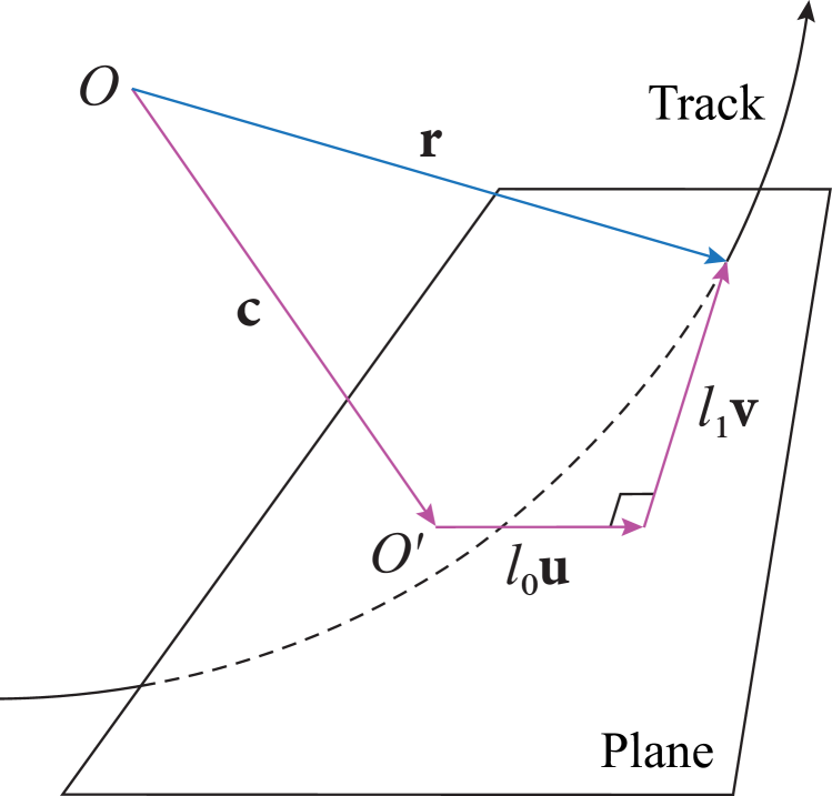
In many tracking detectors, the local track parameters need to be described on planar surfaces. The frame used to describe such planar surfaces is referred to a bound frame whose and are defined on the plane. The track representation of Eq.4 on the bound frame is illustrated in Fig.1. The condition for the surface intersection is met when the vector from the origin of the local coordinate system to the track position, i.e., (), is on the plane and perpendicular to the surface normal vector (), which is defined as . The condition can be represented as the implicit function of Eq.14:
(20)
The origin of the local coordinate system can be any point on the plane, which will satisfy the implicit condition of Eq.20, and of and will be set accordingly.
Figure 1: Track parametrization for the bound frame where and represent the origins of the global and local coordinate systems, respectively.
For the coordinate transformation Jacobian matrices of Section3, and can be obtained from Eqs.5 and 4 using the fact that , , and are independent of and :
(21)
It is easy to confirm that is the right inverse of in case the coordinate transforms occur at the same position of the same surface.
The remaining off-diagonal sub-matrices are zero matrices because of Eq.4 and of Eq.5 of the bound frame are independent of , and . Thus, and are simplified into block diagonal matrices:
(22)
It is straightforward to confirm that
is the right inverse of , which preserves the covariance matrix after for the local-to-global-to-local transformation on the same frame.
In order to calculate for the bound frames, it is sufficient to obtain from Eq.20:
(23)
where is the normal vector of the final surface. The above equation can be put into Eq.18 with Eq.19:
(24)
diverges when the track intersects surface almost parallel to its plane, where even a very small variation of track parameter at the initial surface can affect a large offset to the intersection points at the final surface.
3.2 Perigee frame
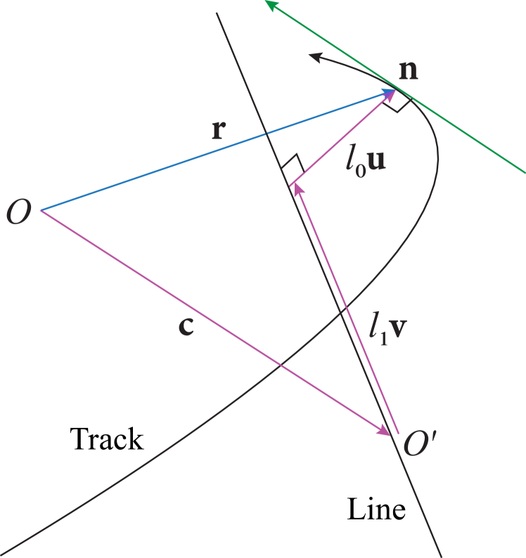
The perigee frame [10] provides a track parametrization to describe the distance between a track and a surface in the form of a straight line. This track parametrization is useful for the vertex reconstruction and wire measurements of straw trackers and drift chambers where the closest approach between the track and a straight line needs to be found. The track representation of the perigee frame based on Eq.4 is illustrated in Fig.2. Here is a unit vector parallel to the line direction and is perpendicular to such that is the distance between the track and the line. This condition can be represented as the implicit function of Eq.14:
(25)
where Eqs.4 and 5 are used to represent as a function of . The origin of the local coordinate system must lie along the line to maintain orthogonality between and . This one-dimensional translation of the origin of the local coordinate system along the line sets and accordingly while remains invariant. In this paper, we define as follows to satisfy the condition of Eq.25:
(26)
where the sign of follows the sign of . There are a few differences in the perigee frame definition between this paper and [10], such as the sign convention and a constant multiplier, but the basic principle remains the same.
Figure 2: Track parametrization for the perigee frame where and represent the origins of the global and local coordinate systems, respectively.
For the coordinate transformation Jacobian matrices, Eq.21 holds as for the bound frame. and are zero matrices because of Eq.4 and of Eq.5 are not functions of . That is a zero matrix can be deduced heuristically (see C for the detailed proof): As is fixed, the variation of can be understood as a rotation around to preserve . However, is a nonzero matrix because the intersection point can rotate around while conserving the elements of . In summary, the coordinate transform Jacobian matrices can be written as the following:
(27)
Here, we only present the final form of for (see C for the detailed derivation):
(28)
follows the same equation by replacing with . Like the bound frame, the product of and on the same perigee frame is the identity matrix as is the zero matrix due to the orthogonality between Eq.28 and Eq.21.
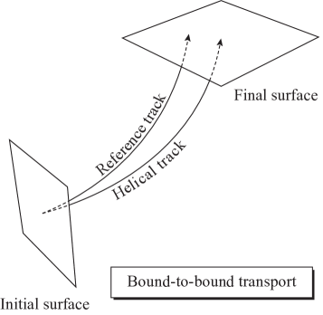
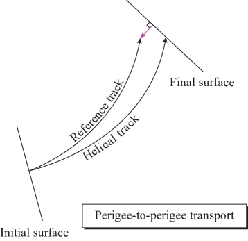
Figure 3: Illustrations of (left) the geometry for the bound-to-bound transport and (right) the geometry for the perigee-to-perigee transport where the helical track is used for the surface construction and the reference track is simulated for the estimation of . The local origins of a surfaces are identical to the local track parameters of the helical track. The helical and reference tracks have the same initial track parameters but the reference track is deviated from the local origin of the final surface under the influence of an inhomogeneous magnetic field and a material. The magenta arrow on the final perigee surface represents the segment of the closest approach, i.e., .
For the derivation of , we can take the same approach as for the bound frame case and obtain from Eq.25:
(29)
where and are the orthonormal basis of the final surface. Substituting into Eq.18 and using Eq.19:
(30)
where .
The exact divergence condition of is complicated, but can be simplified for tracks with small , i.e. on the scale of . This simplification has widespread validity because is limited in a range much smaller than for most experimental setups. For example, a particle with the momentum of in a longitudinal magnetic field has = in the -plane, and the values of for wire measurements are usually in the scale of , such that becomes negligible. Under this assumption, the divergence condition is met when the track is almost parallel to , for the same reason explained in Section3.1.
4 Validation
The derivation of the Jacobian matrices for the bound and perigee frames is validated—following the validation procedure presented in [7]—by simulating muons that propagate from an initial to a final surface in the inhomogeneous magnetic field of the Open Data Detector (ODD) [12, 13] and a uniform material distribution of cesium iodide (CsI). The simulation is executed by the detray library [14] for the track propagation and the covfie library [15] for the linear interpolation of the inhomogeneous magnetic field to arbitrary points. All calculations are performed with 64-bit floating point numbers to maximize precision.
Muons are generated at the origin of the global coordinate system with , and randomly sampled from uniform distributions in the range of [, ], [0, ] and [, ], respectively. To estimate the muon stopping power of the material, only the mean ionization energy loss [16] is considered and the equations used are described in D. Non-Gaussian radiative energy loss such as Bremsstrahlung, and multiple scattering from the Coulomb interaction, which are relatively negligible for the muon momenta of interest [17], are neglected. The representation of their contributions as Jacobian matrices is challenging as discussed in Section5. The and are estimated for these randomly sampled muons, and their trajectories will be called reference tracks with the initial local track parameters of and .
We test geometries consisting of initial and final surfaces which are positioned for the surface-to-surface transport. Tests are performed separately for a geometry with two surfaces with bound frames and a second geometry with two surfaces with perigee frames. The is evaluated for track propagation between two bound frames (bound-to-bound transport) and between two perigee frames (perigee-to-perigee transport). The geometries are illustrated in Fig.3. The reference track is the muon used for the error propagation. The helical track, which has the same initial local track parameters is used to define the local coordinate system of the final surface. The surfaces are re-positioned for every muon depending on the helical trajectory.
The origin of the local coordinate system of the initial surface is set to the origin of the global coordinate system. The origin of the local coordinate system of the final surface is set to the point of intersection with the final surface of the helical track. A homogeneous magnetic field parallel to the -axis with a strength of , which is the average value of the ODD magnetic field, is used to produce the helical tracks. The helical path length from the initial to the final surface is randomly selected from a uniform distribution with a range of [, ]. The of the bound frame is set to the direction of the helical track () at the origin of the local coordinate system, and is set to the curvilinear vector of , namely , where is the unit vector along the -axis. The of the perigee frame is the clockwise -rotation of around . This makes of the perigee frames identical to that of the bound frames.
For generality, we rotate the final surfaces with random Euler angles in the order of local -- axes where the local -axis is and the local -axis is . The first rotation around the local -axis is randomly sampled from a uniform distribution with a range of [0, ]. The second rotation around the new local -axis is performed by randomly sampling the cosine of the angle from a uniform distribution with a range of [, 1], corresponding to the rotation angle in a range of [0, ], and the sign of the rotation angle is also sampled at random. The final rotation around the new local -axis is randomly sampled from a uniform distribution with a range of [0, ]. The initial surfaces are rotated only once around the local -axis in the range of [0, ]. The size of the final surfaces, corresponding to the maximum limits of and , are set 1.5 times larger than the helical path length which is enough to ensure that all tracks intersect the surfaces.
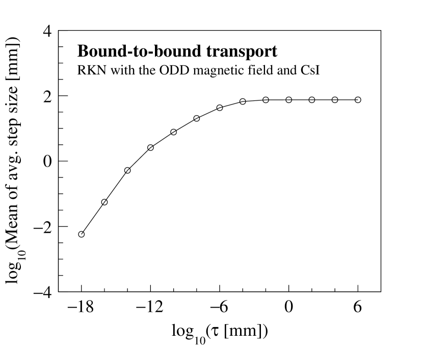
To propagate the tracks between surfaces, we use the adaptive fourth order RKN method [7, 8], as a numerical integration model. This propagates tracks to the final surface in multiple steps with the step size determined by the local error estimate. The local error is estimated by measuring the distance between of the fourth and third order solutions of the current step (see B) [8, 18]. If the local error is larger than error tolerance () the step size is reduced, and vice versa. This means that propagation with a smaller error tolerance proceeds with small steps resulting in a smaller accumulated error at the final surface intersection. The mean values of the step sizes are measured as a function of with the geometry of the bound frames as shown in Fig.4. In addition to the adaptive step size scaling of the RKN method, the step size is limited by the distance to the expected intersection with the surface which is estimated for every step using a straight, tangential ray [14]. The same procedure is repeated until the distance to the surface intersection is less than .
Figure 4: Mean value of the step sizes averaged over reference tracks as a function of the error tolerance . The reference tracks are simulated for the bound-to-bound transport with the ODD magnetic field and CsI.
In Section4.1, we compare the difference between of the reference track and the result of numerical differentiation. We study the difference as a function of to understand its impact on the precision. We repeat the study with the various simulation configurations to investigate the robustness of the Jacobian matrix evaluation against the computation complexity due to magnetic field gradients and energy loss in materials.
In Section4.2, the validation study is extended to the covariance matrix transport because the correctness of Jacobian matrices is not sufficient to justify the first-order Taylor expansion in Eq.7. We attempt to verify that of the reference tracks agrees with the track parameter distributions at the final surface by transporting tracks whose initial parameters are smeared by .
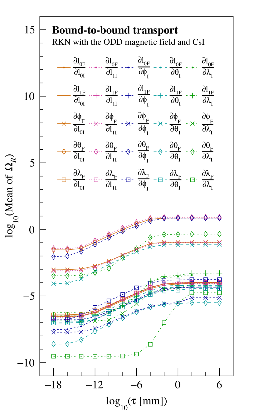
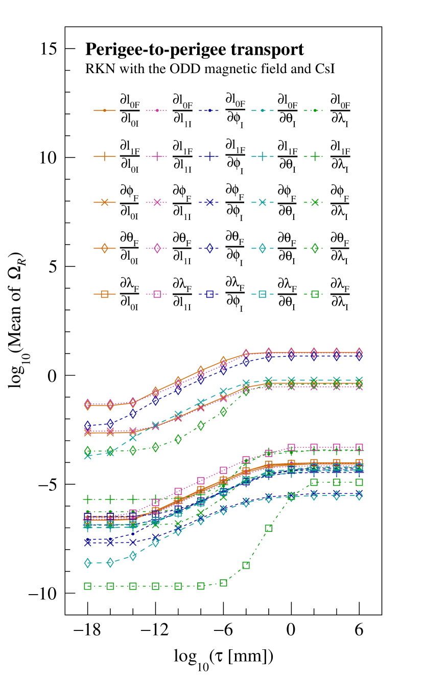
Figure 5: Mean value of for each of elements from (left) bound-to-bound transport and (right) perigee-to-perigee transport with the ODD magnetic field and CsI. The is obtained as a function of of the reference tracks when of the shifted tracks is set to mm.
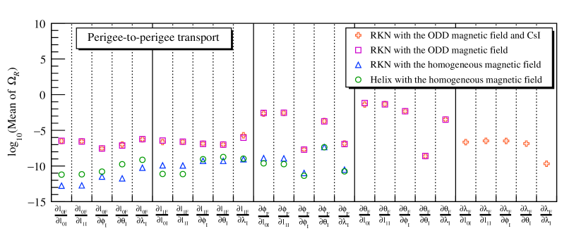
Figure 6: Mean value of for each of the elements from (top) bound-to-bound transport and (bottom) perigee-to-perigee transport with different setups of magnetic fields and materials. The of the reference tracks and the shifted tracks are set to mm and mm, respectively.
4.1 Validation of using numerical differentiation
The numerical differentiation refers to algorithms that numerically calculate the derivative of a function by estimating a change of the function output with respect to a change () of the function input. For the the numerical differentiation, we define a general function that transports local track parameters from the initial surface to the final surface, i.e.:
(31)
where we apply changes of to -th elements of to generate two shifted tracks. These shifted tracks are propagated to the final surface to obtain the local track parameters at the final surface, namely and :
(32)
where is the standard basis where the element at the -th index is one and the other four are zero. We can numerically estimate the element of by calculating a symmetric difference quotient:
(33)
where is the estimation of using the numerical differentiation, and the truncation error is approximately proportional to [18].
To obtain the most precise results from the numerical differentiation, we use an iterative algorithm [18, 19] where we start with a relatively large value of for the evaluation of and decrease it with the rate of for each iteration until we find the accurate solution. At the beginning of every iteration, we perform the numerical differentiation by transporting the shifted tracks to the final surface. A polynomial extrapolation, the Neville’s algorithm [18, 20], is carried out using the results of the previous and current iterations at one order lower, which can be repeated recursively up to the polynomial order equal to the iteration number. We represent the results of the numerical differentiation and polynomial extrapolations with an upper triangle matrix , which is illustrated as follows:
The numerical differentiation at the first row and the polynomial extrapolations are conducted with the following equation:
(34)
The optimal is considered to be with , which has the smallest difference from . The iteration completes when the difference between the highest order extrapolation results of the current and previous iterations is larger than the smallest difference multiplied by a safety factor. In our test, is set to for and , for , for , and for . The is set to 1.2 and the safety factor to 5, which makes most of numerical differentiation complete in a few dozens of iterations.
The metric to estimate the level of agreement between a Jacobian matrix element and the numerical differentiation results, is defined as the residual normalized by the numerical differentiation () [7]:
(35)
The mean values of for all elements of are measured with respect to , as shown in Fig.5. For each value of ranging from to , is evaluated by simulating reference tracks, while is obtained by simulating the shifted tracks with of . Similar behaviors of the residual from the bound-to-bound transport and perigee-to-perigee transport are observed. The smaller than or equal to is not studied because a non-trivial fraction of tracks start failing in finding the final surface due to the precision limit of floating point operation.
The mean values of the residuals under three different configurations of the magnetic field and material are studied. The three configurations are listed with increasing computational complexity: (1) a homogeneous magnetic field with a strength of in the -axis without material, (2) the ODD magnetic field without material, and (3) the ODD magnetic field and CsI, which is the original configuration. The three cases share the surface configuration for the same reference track to compare the precision fairly. The precision of the full-analytical method is also investigated using the helix model [3, 4, 5] for the configuration with the homogeneous magnetic field.
We use an iterative algorithm called the Newton-Raphson method [18] to find the surface intersections of the helical tracks. The helical path length from the initial surface is updated by subtracting the ratio of the expected distance to the final surface and its derivative with respect to the helical path length of the current iteration. As for the semi-analytical method, we use the straight, tangential ray from the current helix position to estimate the distance to the final surface [14], and we repeat the iterations until the distance to the final surface becomes less than .
The mean values of for each configuration are shown in Fig.6 when simulating the reference tracks with of . The derivatives of are not obtained for the configuration with a homogeneous magnetic field in which stays unchanged, and the derivatives of are not obtained for the setups without material for the same reason. For most elements of , the precision decreases with the inhomogeneous magnetic field and the presence of the material does not noticeably impact the precision. As expected, the fourth order RKN method and the analytical helix method obtain similar precision with the homogeneous magnetic field.
Table 1: Gaussian fitting results of pull distributions of tracks simulated with (left) bound-to-bound transport and (right) perigee-to-perigee transport with the ODD magnetic field and CsI. is defined as a chi-square of the Gaussian fitting normalized by the number of degrees of freedom of the fitted data. means the number of the smeared tracks whose pull is larger than 4 or smaller than -4, and is the expected number of such tracks under the assumption of the normal distribution, which is around for tracks. The of the reference tracks and the smeared tracks are set to and , respectively.
Bound-to-bound transport
Value
Mean
Std Dev
0.93
0.47
1.27
0.95
1.04
1.42
1.17
0.79
0.73
1.11
Perigee-to-perigee transport
Value
Mean
Std Dev
0.94
1.11
0.94
0.95
1.15
1.11
1.07
1.58
1.05
1.11
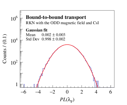
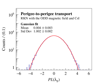
Figure 7: Pull distributions of of (left) bound-to-bound transport and (right) perigee-to-perigee transport with the ODD magnetic field and CsI, fitted by a Gaussian function drawn in red line. The of the reference tracks and the smeared tracks are set to and , respectively.
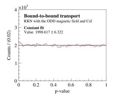
Figure 8: P-value distributions of (left) bound-to-bound transport and (right) perigee-to-perigee transport with the ODD magnetic field and CsI, fitted by a constant function drawn in red line. The of the reference tracks and the smeared tracks are set to and , respectively.
4.2 Validation of covariance matrix transport
To validate Eq.7 statistically, a set of local track parameters at the initial surface smeared from are generated by sampling the displacements at random based on . The smeared tracks are transported to the final surfaces to verify if the distributions of the local track parameters at the final surfaces follow of the reference tracks.
To generate the smeared track parameters, the covariance matrix is decomposed into a lower triangle matrix and its transpose, namely:
(36)
where can be calculated using the Cholesky decomposition. The smeared initial track parameters are generated by adding to the product of and containing elements randomly sampled from the normal distribution [18]:
(37)
The residual between the local track parameters at the final surface transported from and is calculated:
(38)
Each component of is normalized by the standard deviations of to obtain a pull () [7], also known as a standard score:
(39)
If the transport of the covariance matrix with the Jacobian matrix is a good approximation, the distributions of pulls should follow the normal distribution. To demonstrate this, we randomly produce a smeared track of once from a reference track. The reference and smeared tracks are propagated to the final surface to obtain the pulls. For every reference track, is also sampled at random: the square-root of the diagonal elements are randomly sampled from the Gaussian distributions with zero means and the standard deviations of for and , for and , and 10% of for , in accordance with the parameters used in [7]. A correlation factor () is sampled at random from the uniform distribution in the range of [-10%, 10%] and for every off-diagonal element of :
(40)
Once the reference and smeared tracks have been simulated, the pull distributions are fitted with Gaussian functions and their fitted parameters are listed in Table1. For the simulation of the reference tracks including covariance matrix transport, the of is used with feasible computational cost. For the smeared tracks, the of is used as for the numerical differentiation in Section4.1. The mean values and the standard deviations of the fitted Gaussian distributions are close to zero and one, respectively, indicating that the pulls follow the normal distribution. As an example, the pull distributions of with the Gaussian fit are shown in Fig.7.
As a complementary method to qualify the covariance matrix transport with the Jacobian matrix, the randomness of p-value [21], the probability that a sample at least as extreme as the current sample is obtained under the null hypothesis, is studied. The extremeness of the sample can be represented with the chi-square of which is given by:
(41)
The p-value is the upper tail of the chi-squared distribution with the number of degrees of freedom of local track parameters, i.e., five. It is equivalent to the unit subtracted by the value of its cumulative distribution function (CDF) at as follows:
(42)
The p-values are obtained with the same reference and smeared tracks used for the pull distribution tests, and their distributions are shown in Fig.8. Despite the small peak at zero p-value due to the non-linearity of track propagation, the distribution is uniform for all p-values.
5 Discussions
The previous section demonstrated that the Jacobian matrix derived for the error propagation between surfaces works well in the inhomogeneous magnetic field and the homogeneous material. Even though our derivation can also be applied to the inhomogeneous materials, it is not recommended to perform the error propagation over non-uniform materials composition as derivative of stopping power will not be continuous as explained in B. However, in real experiments, the material is typically not homogeneous. For example, in the case of pixel detectors, a particle propagating in the vacuum enters the readout sensor and propagate further inside the sensor, which might have complicated material composition, to reach the point where the measurement occurs. In general, the situation can be simplified by assuming that the sensor has a zero thickness —the thin scatterer approximation [22, 23]— where a covariance matrix corresponding to the energy loss and multiple scattering from the original thickness of material is calculated and added to . In cases where the thin scatterer assumption no longer holds, for example, particles traversing big chunks of materials such as calorimeters, the error propagation can be performed between volume boundaries where each volume is defined for a material chunk. As long as the volume boundaries are smooth enough, it is possible to define a local bound frame tangential to the boundary surface where our formalism of surface-to-surface transport can be applied out of the box.
Only the Cartesian coordinate for the local bound frame has been discussed but detectors can produce measurements with a different coordinate system, e.g., Inner tracker strip sensor of the Phase II upgrade of the ATLAS experiment [24] with a polar coordinate. The additional calculation is done by either transforming the measurement and its error matrix into the local Cartesian coordinate or transforming to the measurement coordinate system and multiplying the additional coordinate transform Jacobian matrix to and .
For the muon simulation, only the mean ionization energy loss is considered, but in reality, the impact of additional effects from the Coulomb scattering and Bremsstrahlung are important for particles with low and ultra-relativistic momentum [11]. The implementation of multiple scattering into Jacobian matrices is challenging due to its randomness as a statistical fluctuations. A workaround is calculating an additional covariance matrix, assuming that the probability density functions of the affected track parameters can be represented as a single or mixture of multiple Gaussian distributions [25, 26], and adding this to the covariance matrix of track parameters. The additional covariance matrix can be obtained for every step of the numerical integration by taking the material per step as a thin scatterer. It is also possible to calculate a single additional covariance matrix [22] for a surface-to-surface transport which is computationally cheaper but less precise. The same method can be applied for Bremsstrahlung whose probability density function of energy loss can also be represented as a mixture of multiple Gaussian distributions [27]. If applicable, the stopping power can be calculated analytically and included in the numerical integration model as done for the mean ionization energy loss explained in D.
Numerical details, such as the selection requirements on or whether to use 32-bit or 64-bit floating point numbers needs to be studied independently for each experiment by investigating not only the computing time but also its impact on the final track fitting results.
6 Summary and conclusions
We have derived Jacobian matrices for the error propagation of charged particles traversing between two surfaces in the presence of inhomogeneous magnetic fields and materials. The local reference frames of the surfaces widely used in high energy physics experiments, namely bound and perigee frames are used. The Jacobian matrix is decomposed into sub-Jacobian matrices corresponding to the coordinate transform and transport in the global coordinate system to facilitate the derivation.
The derivation was validated by simulating track propagation between two surfaces using the fourth order RKN method to perform numerical integration. The derived Jacobians and transported covariance matrices are in good agreement with the results of the numerical methods.
Acknowledgements
We would like to thank Prof. Are Strandlie for valuable comments and encouraging us to publish the results. This work was supported by the National Science Foundation under Cooperative Agreements OAC-1836650, PHY-2323298 and PHY-2120747.
Appendix A Track propagation with a helix model
This provides the equations for the helix propagation model in the global coordinate system and its Jacobian matrices [3, 4, 5] used for the calculation of . The helix propagation is only valid for charged particles traveling in free space with homogeneous magnetic fields and under the assumption that there is no radiative energy loss. The helix model has limited applicability for realistic experiments where the magnetic field is typically inhomogeneous, however, it is used for the validation of semi-analytical models such as the RKN method by crosschecking the results from the propagation, as studied in Section4.
We start by defining the global track parameters at as . The global position along the helical trajectory in the constant magnetic field is given as a function of [3, 4, 5]:
(43)
where and . The direction is simply the derivative of with respect to :
(44)
The Jacobian matrix is represented with block matrices:
(45)
The following identities are useful in deriving with respect to :
(46)
To derive with respect to , the column-wise matrix cross product () is defined using a cross product of each column of matrix with a given vector. For example, a matrix with the columns of and , has a column-wise matrix cross product with a three-element vector defined as follows:
(47)
The column-wise matrix cross product can be applied to the derivative of the cross product between two three-element vectors with respect to another three-element vector:
(48)
which directly provides the following identity:
(49)
The non-zero block matrices of Eq.45 can be derived easily [3, 4, 5] using AppendixA and Eq.49:
(50)
(51)
(52)
(53)
(54)
The of Eq.45 can be used as of Eq.18 because the is an independent parameter.
Appendix B Track propagation with the adaptive fourth order Runge-Kutta-Nyström method
The application of the fourth order RKN method to the track propagation can be found in [6, 7, 8]. This section briefly introduces how the fourth order RKN method advances global track parameters and provide some details on its numerical integration to calculate .
B.1 Advancing global track parameters per step
The RKN method numerically integrates and with a given step size of accumulated in to solve the second order differential equation Eq.1, namely :
(55)
where the quotation mark denotes the partial derivative with respect to , thus, is equivalent to .
For every step of the fourth order RKN method, the global track parameters are calculated at four different stages to evaluate Eq.1, namely [9, 28]:
(56)
where , , and represent the global track parameters of the current step, and the parameters at the four stages of each step have the subscripts of 1, 2, 3, and 4. It should be noted that is evaluated as follows:
(57)
Before evaluating , in the presence of materials, should be known by calculating at and . We use the fourth order Runge-Kutta method [18] to evaluate them as done in [6]:
(58)
where is given by:
(59)
and are directly provided in SectionB.1, which can be recursively obtained by calculating of the previous stage. The positions, and are the same, as are and .
The global track parameters for the next step are estimated as follows [6]:
(60)
In the validation tests of Section4, is normalized for each step to ensure that it is always the unit vector.
The local error (), the absolute difference between of the fourth and third order RKN method, is estimated as follows [8]:
(61)
The next step size () is scaled with the ratio of the error tolerance and local error estimation [8]:
(62)
which is constrained between and to prevent a drastic change in the step size.
B.2 Calculation of
We start by defining a step Jacobian matrix () for the propagation from to corresponding to a single step of the RKN method:
(63)
If the track propagation makes steps to reach the final surface from the initial surface, can be integrated using the Bugge-Myrheim method [6, 7] as follows:
(64)
where is the step Jacobian matrix of the -th step.
Each block matrices of can be expanded using SectionB.1:
(65)
can be calculated using the column-wise matrix cross product defined in AppendixA:
(66)
where a chain rule is applied to given that inhomogeneous magnetic fields are a function of the positions, and the magnetic field gradients at can be obtained using the numerical differentiation. The term with is neglected here, which is zero in the case of the homogeneous material configuration. This term is non-zero in the case a track propagates through inhomogeneous materials between two surfaces but such a configuration is rarely used in the experimental software. Typically, the covariance matrices are transported within the same material by dividing geometry volumes appropriately.
Eq.66 can be expanded as follows using the expressions of and of SectionB.1:
(67)
where can be calculated recursively. is calculated in the similar way:
In case the gradients of the magnetic field are small enough, the terms of SectionsB.2 and B.2 can be neglected for the fast software implementation.
Appendix C Solution of and in the perigee frame
In this section, we prove that is a zero matrix and derive of Eq.28 in a complete manner.
C.1 Proof of
The subscripts of will be omitted because the derivation is valid for any surface intersection. We can start by calculating the derivative of Eq.5 with respect to :
(76)
can be expanded by the chain rule and the column-wise cross product, , defined in AppendixA:
(77)
can be detailed as follows:
(78)
Using SectionsC.1 and C.1, we can show that of Eq.76 is also the zero matrix:
(79)
C.2 Derivation of
We will omit the subscripts of because the derivation is valid for any surface intersection. Here are several equations useful for the derivation:
(80)
where is an angle between and in the range of .
From the unit vector condition of , it is easy to derive the orthogonality between and its derivative with respect to :
(81)
The triple cross product of satisfies the following relation:
(82)
Using the above equations, we can derive by starting from Eq.4. As the derivatives of the last two terms of Eq.4 with respect to is zero, can be simplified as follows:
(83)
Application of SectionC.2 to the above equation leads to the following:
(84)
We can add a dummy term using Eq.81 and further simplify the expression using Eq.82:
(85)
The derivative can be finalized by permuting the three vectors in the round brackets.
(86)
Appendix D Mean ionization energy loss and its derivative with respect to
In this section, the equations for the mean ionization energy loss of muons are enumerated [11] and their derivatives with respect to are solved.
Table 2: Definitions of variables for the mean ionization energy loss.
Type
Symbol
Definition
constant
electron mass of
absorbermaterialproperty
mass density
mean excitation energy
atomic number
atomic molar mass
incidentparticleproperty
charge number
mass
the ratio of speed and
Lorentz factor
maximum possible energy transferto an electron in a single collision
etc.
density effect correction
D.1 Mean ionization energy loss
The mean energy loss per path length of charged particles which are relativistic () and heavy is described by the Bethe equation [16]:
(87)
where the definitions of variables are listed in Table2. The material properties of , , , and can be found in [29]. is computed by the following equation:
(88)
The density effect correction is obtained by [30]:
(89)
where is the parametrization of , and the density effect data of (, , , , , and ) for each material can also be found in [29].
D.2 Derivation of
The derivative of with respect to is as follows:
(90)
Using the above equation, it is trivial to obtain the derivatives of and :
(91)
(92)
The derivative of is calculated using Eqs.91 and 92:
(93)
The derivative of mean ionization energy loss is calculated using SectionsD.2, 92 and D.2:
(94)
where is given by:
(95)
References
[1]
R. E. Kalman, A New Approach to Linear Filtering and Prediction Problems, Journal of Basic Engineering 82 (1) (1960) 35–45.
[2]
R. Frühwirth, Application of Kalman filtering to track and vertex fitting, Nucl. Instr. and Meth. A 262 (2) (1987) 444–450.
[3]
W. Wittek, Transformation of error matrices for different sets of variables which describe a particle trajectory in a magnetic field, Tech. rep., CERN, Geneva (1980).
[4]
W. Wittek, Error propagation along a helix, Tech. rep., CERN, Geneva (1981).
[5]
A. Strandlie, W. Wittek, Derivation of Jacobians for the propagation of covariance matrices of track parameters in homogeneous magnetic fields, Nucl. Instr. and Meth. A 566 (2) (2006) 687–698.
[6]
L. Bugge, J. Myrheim, Tracking and track fitting, Nuclear Instruments and Methods 179 (2) (1981) 365–381.
[7]
E. Lund, L. Bugge, I. Gavrilenko, A. Strandlie, Transport of covariance matrices in the inhomogeneous magnetic field of the ATLAS experiment by the application of a semi-analytical method, JINST 4 (04) (2009) P04016.
[8]
E. Lund, L. Bugge, I. Gavrilenko, A. Strandlie, Track parameter propagation through the application of a new adaptive Runge-Kutta-Nyström method in the ATLAS experiment, JINST 4 (04) (2009) P04001.
[9]
E. Nyström, Über die numerische Integration von Differentialgleichungen, Acta Societatis scientiarum Fennicae, Druck der Finnischen literaturgesellschaft, 1925.
[10]
P. Billoir, S. Qian, Fast vertex fitting with a local parametrization of tracks, Nucl. Instr. and Meth. A 311 (1) (1992) 139–150.
[11]
R. L. Workman, et al., Review of Particle Physics, PTEP 2022 (2022) 083C01.
[12]
P. Gessinger-Befurt, A. Salzburger, J. Niermann, The Open Data Detector Tracking System, Journal of Physics: Conference Series 2438 (1) (2023) 012110.
[13]
C. Allaire, P. Gessinger, J. Hdrinka, M. Kiehn, F. Kimpel, J. Niermann, A. Salzburger, S. Sevova, OpenDataDetector (Apr. 2022).
doi:10.5281/zenodo.6445359.
[14]
A. Salzburger, J. Niermann, B. Yeo, A. Krasznahorkay, Detray: a compile time polymorphic tracking geometry description, Journal of Physics: Conference Series 2438 (1) (2023) 012026.
[15]
S. N. Swatman, A.-L. Varbanescu, A. Pimentel, A. Salzburger, A. Krasznahorkay, Systematically Exploring High-Performance Representations of Vector Fields Through Compile-Time Composition, in: Proceedings of the 2023 ACM/SPEC International Conference on Performance Engineering, ICPE ’23, Association for Computing Machinery, New York, NY, USA, 2023, p. 55–66.
[16]
H. Bethe, Zur Theorie des Durchgangs schneller Korpuskularstrahlen durch Materie, Annalen der Physik 397 (3) (1930) 325–400.
[17]
D. E. Groom, N. V. Mokhov, S. I. Striganov, MUON STOPPING POWER AND RANGE TABLES 10 MeV–100 TeV, Atomic Data and Nuclear Data Tables 78 (2) (2001) 183–356.
[18]
W. H. Press, S. A. Teukolsky, W. T. Vetterling, B. P. Flannery, Numerical Recipes 3rd Edition: The Art of Scientific Computing, 3rd Edition, Cambridge University Press, 2007.
[19]
C. Ridders, Accurate computation of F′(x) and F′(x) F(x), Advances in Engineering Software (1978) 4 (2) (1982) 75–76.
[20]
E. H. Neville, Iterative interpolation, St. Joseph’s IS Press, 1934.
[21]
Y.-L. T. Duncan J Murdoch, J. Adcock, P-Values are Random Variables, The American Statistician 62 (3) (2008) 242–245.
doi:10.1198/000313008X332421.
[22]
R. Frühwirth, M. Regler, R. K. Bock, H. Grote, D. Notz, Data analysis techniques for high-energy physics; 2nd ed., Cambridge monographs on particle physics, nuclear physics, and cosmology, Cambridge Univ. Press, Cambridge, 2000.
[23]
R. Frühwirth, A. Strandlie, Pattern Recognition, Tracking and Vertex Reconstruction in Particle Detectors, Springer Cham, 2021.
[24]
N. Hessey, Building a Stereo-angle into strip-sensors for the ATLAS-Upgrade Inner-Tracker Endcaps, Tech. rep., CERN, Geneva (2013).
[25]
V. L. Highland, Some practical remarks on multiple scattering, Nuclear Instruments and Methods 129 (2) (1975) 497–499.
[26]
G. R. Lynch, O. I. Dahl, Approximations to multiple Coulomb scattering, Nuclear Instruments and Methods in Physics Research Section B: Beam Interactions with Materials and Atoms 58 (1) (1991) 6–10.
[27]
R. Frühwirth, A Gaussian-mixture approximation of the Bethe–Heitler model of electron energy loss by bremsstrahlung, Computer Physics Communications 154 (2) (2003) 131–142.
[28]
M. Abramowitz, I. A. Stegun (Eds.), Handbook of Mathematical Functions with Formulas, Graphs, and Mathematical Tables, tenth printing Edition, U.S. Government Printing Office, Washington, DC, USA, 1972.