Unveiling clean two-dimensional discrete time quasicrystals on a digital quantum computer

Abstract

In periodically driven (Floquet) systems, evolution typically results in an infinite-temperature thermal state due to continuous energy absorption over time. However, before reaching thermal equilibrium, such systems may transiently pass through a meta-stable state known as a prethermal state. This prethermal state can exhibit phenomena not commonly observed in equilibrium, such as discrete time crystals (DTCs), making it an intriguing platform for exploring out-of-equilibrium dynamics. Here, we investigate the relaxation dynamics of initially prepared product states under periodic driving in a kicked Ising model using the IBM Quantum Heron processor, comprising 133 superconducting qubits arranged on a heavy-hexagonal lattice, over up to $100$ time steps. We identify the presence of a prethermal regime characterised by magnetisation measurements oscillating at twice the period of the Floquet cycle and demonstrate its robustness against perturbations to the transverse field. Our results provide evidence supporting the realisation of a period-doubling DTC in a two-dimensional system. Moreover, we discover that the longitudinal field induces additional amplitude modulations in the magnetisation with a period incommensurate with the driving period, leading to the emergence of discrete time quasicrystals (DTQCs). These observations are further validated through comparison with tensor-network and state-vector simulations. Our findings not only enhance our understanding of clean DTCs in two dimensions but also highlight the utility of digital quantum computers for simulating the dynamics of quantum many-body systems, addressing challenges faced by state-of-the-art classical simulations.

Periodically driven (Floquet) systems host novel phases of matter inaccessible in thermal equilibrium. Notably, discrete time crystals (DTCs) [1, 2, 3, 4, 5] represent genuine out-of-equilibrium phases of matter [6, 7, 8, 9] feasible in Floquet systems [10, 11, 12]. A DTC is characterised by subharmonic responses breaking discrete time-translational symmetry imposed by the periodic drive. However, sustaining DTCs as transient meta-stable states faces challenges due to thermalisation, where many-body interactions drive low-entangled states to highly entangled, high-energy states. Overcoming this obstacle requires imparting a many-body localised nature to the dynamics.

One strategy to circumvent rapid thermalisation in driven systems is by introducing disorder in the Floquet Hamiltonian, inducing many-body localisation (MBL) to break ergodicity [11, 12, 13, 14, 15]. Recently, disorder-induced MBL-based DTCs (MBL-DTCs) have been demonstrated on digital quantum computers in one dimension [16, 17, 18]. Furthermore, topological time crystalline order has been achieved in a periodically driven disordered toric code on a superconducting quantum computer [19]. Another avenue for DTCs involves the prethermal regime of periodically driven clean systems in two or higher dimensions [20, 21, 22, 23, 24, 25, 26, 27]. Unlike MBL-DTCs, prethermal DTCs are not stabilised in one-dimensional systems with short-range interactions, aligning with the absence of symmetry breaking at finite temperatures in one dimension. Therefore, realising a clean prethermal DTC requires two or higher dimensions, or otherwise long-range interactions.

In simulating dynamics of quantum many-body systems in two dimensions, tensor-network methods have been extensively utilised for large systems beyond the capabilities of state-vector simulations [28, 29, 30, 3]. However, accurate tensor-network simulations over extended periods become challenging in two dimensions due to breakdowns in low-rank tensor approximations when entanglement exceeds certain thresholds dictated by bond dimensions. Conversely, recent advancements in noisy intermediate-scale quantum devices have introduced digital quantum computers as another tool to investigate out-of-equilibrium phases of matter, including DTCs. Indeed, a recent study has observed indications of clean DTCs in two dimensions using a digital quantum computer [32]. Nevertheless, the previous study has been performed on systems of a few tens of qubits, leaving large-scale digital quantum simulations, comparable to state-of-the-art classical tensor-network simulations, of clean DTCs to examine their stability in two dimensions.

Here, we demonstrate the realisation of clean DTCs on a two-dimensional heavy-hexagonal lattice of $133$ qubits (see Fig. 1a) using an IBM Quantum Heron processor, ibm_torino. By applying periodic driving to initial product states in a kicked Ising model, involving both transverse and longitudinal fields, we measure local magnetisation to observe its subharmonic response. With a simple error mitigation protocol based on a depolarising noise model, our results are first validated by showing agreement with both tensor-network simulations of the $133$-qubit system and state-vector simulations of a $28$-qubit system for up to $50$ time steps. We then observe a subharmonic period-doubling response of local magnetisation persisting for at least $100$ time steps, confirming its stability against perturbations to the transverse field, which thereby provides evidence for a realisation of clean DTCs in two dimensions. Furthermore, we observe other longer-period subharmonic responses with frequencies incommensurate with the driving period, thus identified as discrete time quasicrystals (DTQCs) [22, 25].

We explore the Floquet dynamics of a kicked Ising model on an $L$-qubit system governed by a time-dependent Hamiltonian of period $T$, satisfying $\hat{H}(t)=\hat{H}(t+T)$ with

$$\hat{H}(t)=\left\{\,\begin{aligned} &h_{x}\sum_{i=0}^{L-1}\hat{X}_{i},&\text{ for }0\leqslant t<T/2\\ &h_{z}\sum_{i=0}^{L-1}\hat{Z}_{i}-J\sum_{\langle i,j\rangle}\hat{Z}_{i}\hat{Z}_{j}&\text{ for }T/2\leqslant t<T\end{aligned}\right.,$$ (1)

where $\hat{X}_{i}$ and $\hat{Z}_{i}$ are Pauli operators at qubit $i$, and $\sum_{i}$ and $\sum_{\langle i,j\rangle}$ run over all vertices and edges of the lattice, respectively. $h_{x}$, $h_{z}$, and $J$ are parameters, referred to as the transverse field, longitudinal field, and exchange interaction, respectively. The associated single-cycle Floquet operator $\hat{U}_{\text{F}}$ can be expressed in terms of single- and two-qubit gates as

$$\hat{U}_{\text{F}}=\left[\prod_{i}\hat{R}_{Z_{i}}(\theta_{z})\right]\left[\prod_{\langle i,j\rangle}\hat{R}_{Z_{i}Z_{j}}(\theta_{J})\right]\left[\prod_{i}\hat{R}_{X_{i}}(\theta_{x})\right],$$ (2)

where $\hat{R}_{Z_{i}Z_{j}}(\theta_{J})=\exp\left[-\mathrm{i}\theta_{J}\hat{Z}_{i}\hat{Z}_{j}/2\right]$, $\hat{R}_{Z_{i}}(\theta_{z})=\exp\left[-\mathrm{i}\theta_{z}\hat{Z}_{i}/2\right]$, and $\hat{R}_{X_{i}}(\theta_{x})=\exp\left[-\mathrm{i}\theta_{x}\hat{X}_{i}/2\right]$ are $ZZ$, $Z$, and $X$ rotation gates with rotation angles $\theta_{J}=-JT$, $\theta_{z}=h_{z}T$, and $\theta_{x}=h_{x}T$, respectively. Since each qubit is coupled to at most three adjacent qubits on the heavy-hexagonal lattice, operation of all the two-qubit gates $\hat{R}_{Z_{i}Z_{j}}(\theta_{J})$ has to be divided into three layers (see Fig. 1b). Each layer consists of $\hat{R}_{Z_{i}Z_{j}}(\theta_{J})$ gates on red, blue, or green edges in Fig. 1a, allowing for parallel operation.

The time-evolved state at stroboscopic times $t=nT$ with integer $n$ is expressed as $|\psi(t)\rangle=(\hat{U}_{\rm F})^{n}|\psi(0)\rangle,$ where $|\psi(0)\rangle$ represents the initial state. Our primary focus lies in measuring local magnetisation defined as $\langle\hat{Z}_{j}(t)\rangle=\langle\psi(t)|\hat{Z}_{j}|\psi(t)\rangle,$ where $\hat{Z}_{j}(t)=(\hat{U}_{\rm F}^{\dagger})^{n}\hat{Z}_{j}(\hat{U}_{\rm F})^{n}$ is the Heisenberg representation of the Pauli $\hat{Z}_{j}$ operator, and $\langle\cdots\rangle=\langle\psi(0)|\cdots|\psi(0)\rangle$ denotes the expectation value with respect to the initial state. The initial state is prepared as a product state in the computational basis, forming a stripe pattern of $|0\rangle$’s and $|1\rangle$’s, represented by white and black circles in Fig. 1a. Among the three independent model parameters, we set $\theta_{J}=-\pi/2$ and vary the other two parameters $\theta_{x}$ and $\theta_{z}$. The gate $\hat{R}_{Z_{i}Z_{j}}(\theta_{J})$ at $\theta_{J}=-\pi/2$ is decomposed into the CZ gate, the native two-qubit gate of ibm_torino, and the $S$ gate, as $\hat{R}_{Z_{i}Z_{j}}(-\pi/2)=e^{i\pi/4}\widehat{\rm CZ}_{ij}(\hat{S}_{i}^{\dagger}\otimes\hat{S}_{j}^{\dagger})$.

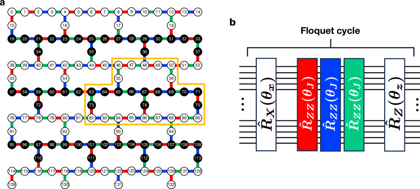
Figure 1: Two-qubit gate connectivity on a heavy-hexagonal lattice and initial product states. a, The overall device geometry of ibm_torino, comprising a hevey-hexagonal lattice of $L=133$ qubits. Each circle represents a qubit and the edges indicate the qubit connectivity. Three layers of $R_{ZZ}$ gates in a single Floquet circle are highlighted in red, blue, and green (also see b). The enclosed area marked by the yellow line represents the system of $L=28$ qubits, utilised for comparison with state-vector simulations. The initial state is prepared as a product state with qubits denoted by white (black) circles initialised to be $|0\rangle$ ($|1\rangle$). b, Schematic representation of the single-cycle Floquet operator $\hat{U}_{\rm F}$. The red, blue, and green boxes correspond to the three layers of $R_{ZZ}$ gates, each applied in parallel, indicated in a, while the white boxes represent the products of $R_{X}$ and $R_{Z}$ gates. The horizontal lines represent the qubits on which the quantum gates operate.

For convenience, we introduce a perturbation parameter $\epsilon$ to the transverse field as $2\epsilon=\pi-\theta_{x}.$ When $\varepsilon=0$, the dynamics of $\hat{Z}_{j}(t)$ becomes trivial because a single Floquet cycle simply flips the sign of the local magnetisation, $\hat{Z}_{j}(t+T)=\hat{U}_{\rm F}\hat{Z}_{j}(t)\hat{U}_{\rm F}^{\dagger}=(-1)\hat{Z}_{j}(t)$. This demonstrates that a period-doubling DTC with $|\langle\hat{Z}_{j}(t)\rangle|=1$ is realised, at least at the fine-tuned parameter $\theta_{x}=\pi$. Our primary interest therefore lies in the subharmonic response of the magnetisation for $\epsilon>0$.

We utilise ibm_torino, the IBM Quantum Heron processor comprising $133$ superconducting qubits arranged on the heavy-hexagonal lattice (see Fig. 1a) [33]. The median infidelity of the native two-qubit gates (i.e., CZ gates) is approximately $4\times 10^{-3}$, while the infidelity of single-qubit gates is around $4\times 10^{-4}$ with the median read-out error of $1.7\times 10^{-2}$ (see also Supplementary Information S1). Each Floquet cycle involves $150$ CZ gates for the $L=133$ system, totaling $150n$ CZ gates for $n$ time steps. Given the three non-parallelisable layers of two-qubit gates per cycle, the circuit depth for the $n$ time steps is $3n$. Considering a two-qubit gate time of about $100$ns, the real-time duration from state preparation to final measurement for the maximum circuit depth $300$ for $n=100$ is estimated as roughly $30\mu$s, significantly shorter than the median single-qubit coherence times $T_{1}=165\mu$s and $T_{2}=138\mu$s.

First, we introduce an error-mitigation scheme to validate that the quantum device provides reliable results for magnetisation dynamics. We measure the time evolution of the averaged magnetisation over a set of qubits,

$${\hat{Z}_{\rm avg}}(t)=\frac{1}{|A|}\sum_{j\in A}\hat{Z}_{j}(t),$$ (3)

where $|A|$ denotes the number of qubits in set $A$, and we choose that $A=\{63,64,65,66,67,68,69,70,71\}$ for the $L=28$ system and $A=\{57,58,59,60,61,62,63,64,65,66,67,68,69,70,71\}$ for the $L=133$ system (see Fig. 1a). In utilising the quantum device, we estimate the expectation value of ${\hat{Z}_{\rm avg}}(t)$ at each time step by computing the sample mean of outcomes from projective measurements on all qubits within $A$ in the computational basis over $2^{14}$ samples. The statistical error associated with this estimate is determined as the sample standard deviation of the mean. The results are shown in Fig. 2a,c, where neither error-suppression methods such as dynamical decoupling [34, 35] nor error-mitigation methods such as zero-noise extrapolation [36, 37] and probabilistic error cancellation [38] are used (the same holds for the other results presented below).

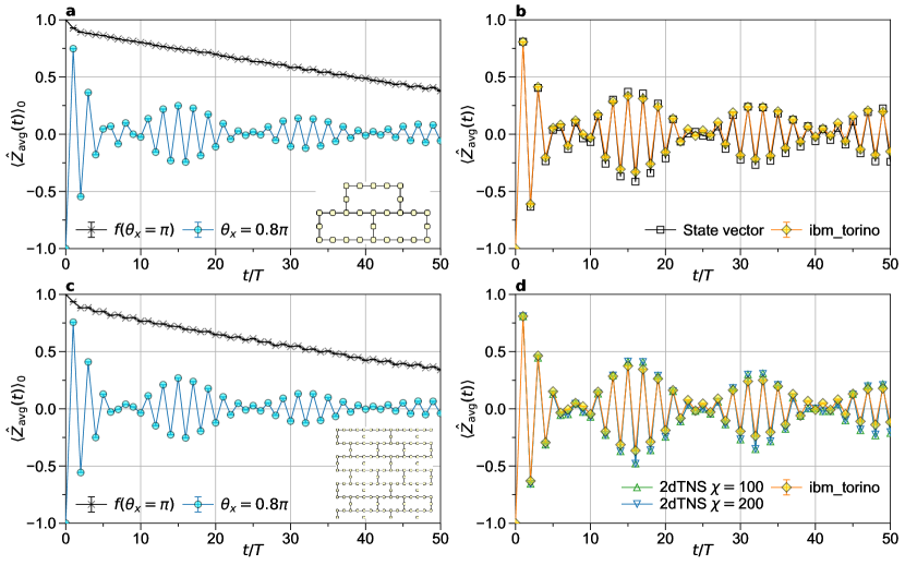
Figure 2: Error-mitigation protocol and comparison with classical simulations. a, Raw data of the averaged magnetisation $\langle\hat{Z}_{\rm avg}(t)\rangle_{0}$ at $(\theta_{x},\theta_{z})=(0.8\pi,0.5\pi)$ (cyan circles) and $f(\theta_{x}=\pi)=|\langle\hat{Z}_{\rm avg}(t)\rangle_{0,\theta_{x}=\pi}|$ at $(\theta_{x},\theta_{z})=(\pi,0.5\pi)$ (black crosses) for $L=28$. b, Error-mitigated data (yellow diamonds) of the averaged magnetisation $\langle\hat{Z}_{\rm avg}(t)\rangle$ at $(\theta_{x},\theta_{z})=(0.8\pi,0.5\pi)$ for $L=28$. Numerically exact results obtained by state-vector simulations are also shown with black squares in b. c-d, Same as a-b but for $L=133$. Results of classical tensor-network simulations with bond dimensions $\chi=100$ and 200 are also shown with green and blue triangles, respectively, in d. Error bars in b and d represent the propagated error due to sampling errors in the quantities in the numerator and the denominator of Eq. (4).

As described above, at $\theta_{x}=\pi$, the noiseless expectation value satisfies $|\langle\hat{Z}_{\rm avg}(t)\rangle|=1$. However, the absolute values of the raw data obtained from the quantum device, denoted as $f(\theta_{x}=\pi):=|\langle\hat{Z}_{\rm avg}(t)\rangle_{0}|$, deviate from the ideal value $1$, with the deviation increasing over time steps, as observed in Fig. 2a,c. To account for this signal decay, we introduce a global depolarising noise model, where the expectation value $\langle\hat{O}(t)\rangle_{0}$ of an observable $\hat{O}$ subject to depolarising noise is given by $\langle\hat{O}(t)\rangle_{0}=f\langle\hat{O}(t)\rangle+(1-f){\rm Tr}[\hat{O}(t)]/2^{L}$ [39, 40]. Here, $f$ is a parameter that characterises the depolarising noise model, with $\langle\hat{O}(t)\rangle$ representing the ideal expectation value of $\hat{O}$ and ${\rm Tr}[\hat{O}(t)]/2^{L}$ being the expectation value over the maximally mixed state. Generally, $f$ depends on both the circuit and observable, i.e., $f=f(\theta_{J},\theta_{x},\theta_{z},n,\hat{O})$. Since $|\langle\hat{Z}_{\rm avg}(t)\rangle|=1$ at $\theta_{x}=\pi$ and ${\rm Tr}[\hat{Z}_{\rm avg}(t)]=0$ as $\hat{Z}_{j}(t)$ is traceless, the parameter $f$ can be estimated in this trivial case as $f(\theta_{J},\pi,\theta_{z},n,\hat{Z}_{\rm avg})=|\langle\hat{Z}_{\rm avg}(t)\rangle_{0,\theta_{x}=\pi}|$, where $\langle\hat{Z}_{\rm avg}(t)\rangle_{0,\theta_{x}=\pi}$ is $\langle\hat{Z}_{\rm avg}(t)\rangle_{0}$ obtained at $\theta_{x}=\pi$. For general $\theta_{x}$, it is difficult to estimate $f$ because the ideal expectation value $\langle\hat{Z}_{\rm avg}(t)\rangle$ is not available. To circumvent this issue, we approximate $f(\theta_{J},\theta_{x},\theta_{z},n,\hat{Z}_{\rm avg})$ by $f(\theta_{J},\pi,\theta_{z},n,\hat{Z}_{\rm avg})=f(\theta_{x}=\pi)$. This approximation leads to an error mitigation scheme:

$$\langle\hat{Z}_{\rm avg}(t)\rangle\approx\frac{\langle\hat{Z}_{\rm avg}(t)\rangle_{0}}{|\langle\hat{Z}_{\rm avg}(t)\rangle_{0,\theta_{x}=\pi}|}.$$ (4)

Similar error-mitigation protocols have been successfully applied previously to correct magnetisation [18] and out-of-time-ordered correlators [41].

The raw data $\langle\hat{Z}_{\rm avg}(t)\rangle_{0}$ for the $L=28$ qubit system at $(\theta_{x},\theta_{z})=(0.8\pi,0.5\pi)$ are displayed in Fig. 2a. These data already capture characteristic oscillations up to 50 time steps, also observed in the state-vector simulation (Fig. 2b). However, similar to the trivial case at $\theta_{x}=\pi$, the signal diminishes with increasing time steps compared to the state-vector simulation results. Employing the error-mitigation protocol introduced in Eq. (4) restores the signal reduction, yielding excellent agreement with the state-vector simulation results up to 50 time steps, as shown in Fig. 2b. Further comparisons for other parameters over the extended time steps up to 100 are found in Supplementary Information S2.

The same error mitigation scheme demonstrates excellent performance even for the $L=133$ system, as shown in Fig. 2c,d. In parallel, we employ a two-dimensional tensor-network state (2dTNS) method as a classical counterpart (Supplementary Information S5). The 2dTNS results presented here converge with respect to the bond dimension $\chi$, which governs the accuracy of the approximation inherent in the 2dTNS method, for time steps up to at least 50 (see Supplementary Information S3 for further comparisons with longer time steps and different parameters). Once again, the remarkable agreement between the error-mitigate data and the converged tensor-network simulation results confirms the reliability of the quantum device outcomes. This validation firmly establishes digital quantum simulations on the quantum device as a compelling tool to explore clean DTCs in two dimensions. It should also be emphasised here that the number of time steps achievable in this quantum device, providing reliable results along with the simple mitigation protocol, easily exceeds that of previous similar dynamics experiments using the IBM Eagle processor of 127 qubits with the median infidelity of two-qubit gates $\sim 1\times 10^{-2}$ [42], where at most 20 time steps were evolved, albeit with various error-mitigation techniques involved.

Having validated the reliability of quantum hardware results, we now delve into discrete time-crystalline orders in two dimensions. Figure 3 shows the long-time dynamics, spanning up to 100 time steps, of the raw and mitigated magnetisation, $\langle\hat{Z}_{\rm avg}(t)\rangle_{0}$ and $\langle\hat{Z}_{\rm avg}(t)\rangle$, respectively, on the heavy-hexagonal lattice of $L=133$ qubits for various sets of parameters $(\theta_{x},\theta_{z})$. Overall, the decay of the magnetisation becomes more pronounced as $\theta_{x}$ decreases. Specifically, period-doubling oscillations persist even around $t/T=100$ for $\theta_{x}\geqslant 0.8$, while they are barely observable for $t/T\gtrsim 20$ at $\theta_{x}=0.7$, suggesting thermalisation. These observations lead to the conclusion that DTCs observed on the heavy-hexagonal lattice remain stable in the range $0.8\pi\leqslant\theta_{x}\leqslant\pi$, where a prethermal plateau [23] is distinctly visible withing the time steps $0\leqslant t/T\leqslant 100$. This is in sharp contrast to the behavior in one dimension, where magnetisation oscillations quickly decay, irrespective of the parameters $(\theta_{x},\theta_{z})$ away from the trivial point at $\theta_{x}=\pi$, as we have also confirmed in Supplementary Information S4 using the same quantum device.

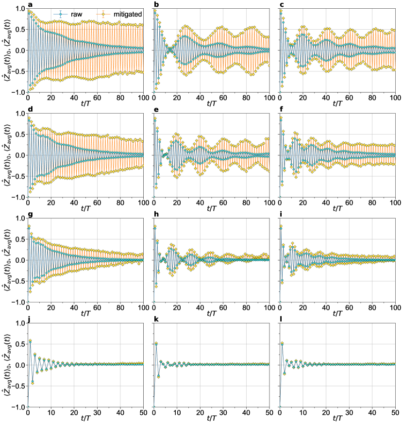
Figure 3: Dynamics of magnetisation exhibiting DTC, DTQC, and thermalisation. The raw data $\langle\hat{Z}_{\rm avg}(t)\rangle_{0}$ (cyan circles) and the error-mitigated data $\langle\hat{Z}_{\rm avg}(t)\rangle$ (yellow diamonds) obtained on the heavy-hexagonal lattice of $L=133$ qubits at various parameter sets $(\theta_{x},\theta_{z})$: a $(0.9\pi,0)$, b $(0.9\pi,0.5\pi)$, c $(0.9\pi,\pi)$, d $(0.85\pi,0)$, e $(0.85\pi,0.5\pi)$, f $(0.85\pi,\pi)$, g $(0.8\pi,0)$, h $(0.8\pi,0.5\pi)$, i $(0.8\pi,\pi)$, j $(0.7\pi,0.0\pi)$, k $(0.7\pi,0.5\pi)$, and l $(0.7\pi,\pi)$. Notice that the time duration in the horizontal axis in j-l is half of that in the other panels.

In addition to the period-doubling oscillation, the longitudinal field $\theta_{z}$ induces a longer-period oscillation, as clearly seen in Fig. 3 (also see Fig. S6). To analyse this additional oscillation, we perform a discrete Fourier transform of the error-mitigated magnetisation, defined as $\tilde{Z}(\omega)=|\frac{1}{n_{\rm max}}\sum_{n=0}^{n_{\rm max}-1}\langle\hat{Z}_{\rm avg}(nT)\rangle e^{-i\omega nT}|$, where $\omega T=2\pi k/n_{\rm max}$ with $k=0,1,\cdots n_{\rm max}-1$ represents the discrete frequency and the number of time steps involved in the Fourier transform is set to $n_{\rm max}=100$. As shown in Fig. 4a-c, when $\theta_{z}=0$, only a single peak at $\omega T/(2\pi)=0.5$ appears in the Fourier spectrum, indicating the presence of the sole period-doubling DTC. Introducing the longitudinal field $\theta_{z}$ leads to the appearance of additional side peaks symmetrically at $\omega_{\pm}$ on both sides of the main peak. These side peaks gradually deviate from the main peak as $\theta_{z}$ increases. Although $\omega_{\pm}T/(2\pi)$ are always rational numbers of the form $k/n_{\rm max}$ by definition, their systematic dependence on $\theta_{z}$ suggests that each of $\omega_{\pm}T/(2\pi)$ will fluctuate around a generally irrational number for a fixed set of parameters when the number of time steps involved in the Fourier transform is varied. The emergence of these side peaks at frequencies $\omega_{\pm}$, which are susceptible to changes in microscopic parameters and essentially incommensurate with the driving period, serves as a signature of a DTQC [22, 25].

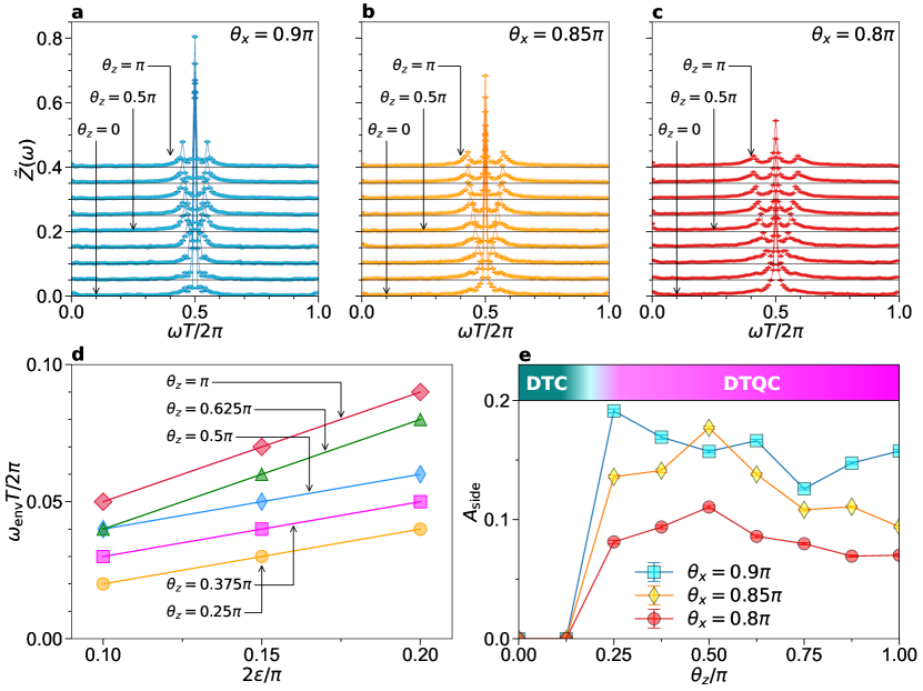
Figure 4: Fourier analysis of DTQC frequencies induced by the longitudinal field. Fourier spectrum $\tilde{Z}(\omega)$ of the averaged magnetisation for a $\theta_{x}=0.9\pi$, b $\theta_{x}=0.85\pi$, and c $\theta_{x}=0.8\pi$ with various values of $\theta_{z}=0,0.125\pi,0.25\pi,\cdots,\pi$ (from bottom to top). The results are offset by 0.05 for adjacent values of $\theta_{z}$ for better visibility. d, Envelope frequency $\omega_{\text{env}}$ of the observed DTQCs as a function of the perturbation parameter $\varepsilon$ to the transverse field. e, Intensity of the side peaks, $A_{\text{side}}$, as a function of $\theta_{z}$. A schematic phase diagram showing the crossover between a DTC and a DTQC is provided at the top of the figure. Error bars in a-c and e represent the propagated error due to sampling errors in $\tilde{Z}(\omega)$. However, they are smaller than the size of symbols.

The envelope frequency of the longer-period DTQC oscillation can be estimated as $\omega_{\text{env}}=(\omega_{+}-\omega_{-})/2$. We observe that the envelope frequency increases proportionally to the perturbation to the transverse field $h_{x}$, i.e., $\omega_{\text{env}}\propto\epsilon$ (Fig. 4d). Particularly at $\theta_{z}=\pi$, $\omega_{\text{env}}T/(2\pi)=0.05$, $0.07$, and $0.09$ for $\theta_{x}=0.9\pi$, $0.85\pi$, and $0.8\pi$, respectively. These values approximately follow $\omega_{\text{env}}T/(2\pi)\simeq\epsilon/(2\theta_{J})$, which is proportional to the frequency of a Bloch oscillation [43] induced by a weak transverse field in a one-dimensional Ising model with long-range interactions [44].

To characterise the crossover between a DTC and a DTQC, we plot the sum of the intensities $A_{\pm}$ of the side peaks at $\omega_{\pm}$, denoted as $A_{\text{side}}=A_{+}+A_{-}$, in Fig. 4e. $A_{\rm side}$ tends to decrease with decreasing $\theta_{x}$. At $\theta_{x}=0.7\pi$, $\langle\hat{Z}_{\rm avg}(t)\rangle$ quickly decays with increasing time step $t/T$ as seen in Figs. 3j-l, indicating the absence of both DTC and DTQC. When $\theta_{x}=\pi$, only the period-doubling DTC is present, as $|\langle\hat{Z}_{\rm avg}(t)\rangle|$ remains 1 regardless of the value of $\theta_{z}$. Therefore, we conclude that DTQCs manifest in a prethermal state persisting within the timescale $0\leqslant t/T\leqslant 100$ for a parameter range of $0.8\pi\lesssim\theta_{x}\lesssim 0.9\pi$ and $0.25\pi\lesssim\theta_{z}\leqslant\pi$.

The recent advancements in the quality of quantum devices have enabled successful simulation of quantum dynamics on a much larger scale, both in terms of qubit count and time step duration. Specifically, achieving quantum dynamics simulation on a 133-qubit system for up to 100 time steps using a digital quantum computer, as demonstrated in this study, represents a significant leap forward compared to previous studies. Our comparative study, employing a 2dTNS method, confirmed the agreement between the results obtained using the quantum device and those from the classical simulations, for approximately up to 50 time steps. However, in our investigation of both 28-qubit and 133-qubit systems, we encountered a critical parameter regime where the perturbation to the transverse field approaches $2\epsilon\approx 0.2\pi$, near the crossover boundary between DTCs/DTQCs and thermalisation. In this regime, the limitation of classical simulations become apparent, particularly for long-time steps around 100. Indeed, in the 28-qubit system, we observe discrepancies between the results of the 2dTNS method, even with the largest feasible bond dimension, and those of the state-vector simulation (Supplementary Information S2). Additionally, in the 133-qubit system, a slow convergence of the results of the 2dTNS method with respect to the bond dimension is observed, implying the growth of entanglement that is hardly tractable within the classical resources available for the 2dTNS method (Supplementary Information S3). These observations highlight the boundary of the classical simulation capabilities. Therefore, our study of Floquet dynamics in this parameter regime, extending up to 100 time steps on the 133-qubit system, pushes the boundaries of classical simulations to their limit, emphasising the significant potential of current digital quantum computers for simulating out-of-equilibrium quantum dynamics in two dimensions.

This work is based on results obtained in part from a project, JPNP20017, subsidised by the New Energy and Industrial Technology Development Organization (NEDO), Japan. We acknowledge the support form the Japan Society for the Promotion of Science (JSPS) KAKENHI Grants (Grant Nos. JP19K23433, JP21H04446, JP22K03479, JP22K03520, and JP23K13066) from the Ministry of Education, Culture, Sports, Science and Technology (MEXT), Japan. We also appreciate the funding received from JST COI-NEXT (Grant No. JPMJPF2221) and the Program for Promoting Research of the Supercomputer Fugaku (Grant No. MXP1020230411) from MEXT, Japan. Furthermore, we acknowledge the support from the UTokyo Quantum Initiative, the RIKEN TRIP project, and the COE research grant in computational science from Hyogo Prefecture and Kobe City through the Foundation for Computational Science. Tensor-network simulations are based on the high-performance tensor computing library GraceQ/tensor [45]. A part of the numerical simulations has been performed using the HOKUSAI supercomputer at RIKEN and the supercomputer Fugaku installed at RIKEN Center for Computational Science.

Supplementary Information to “Unveiling clean two-dimensional discrete time quasicrystals on a digital quantum computer”

S1 Quantum device conditions

The experimental data presented in this study were obtained using the IBM Quantum Heron processor, ibm_torino, via cloud access, predominantly during the period from January 1 to January 31, 2024. Throughout this duration, the average relaxation and coherence times $T_{1}$ and $T_{2}$, as well as the average readout assignment error rate, across all qubits were 165$\mu$s, 138$\mu$s, and 0.03, respectively. Additionally, the average error rate of CZ gates and the average duration of CZ gates across all qubits were 0.006 and 101ns, respectively. Notably, no significant deviations were observed in the data obtained on different dates, indicating the consistency and stability of the quantum device utilised for this study.

S2 Results for a heavy-hexagonal lattice of $L=28$ qubits

Figure S1 shows the error-unmitigated raw data of the averaged magnetisation $\langle\hat{Z}_{\rm avg}(t)\rangle_{0}$ for up to 100 time steps obtained for the $L=28$ system using ibm_torino (see Fig. 1a). Here, the average is performed over the same set $A$ of qubits as described in the main text, i.e., $A=\{63,64,65,66,67,68,69,70,71\}$. To mitigate errors in the raw data for $\theta_{x}\neq\pi$, the results for the trivial cases with $\theta_{x}=\pi$ are utilised, as detailed in Eq. (4).

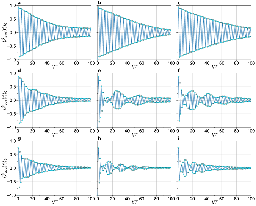
Figure S1: Error-unmitigated raw data $\langle\hat{Z}_{\rm avg}(t)\rangle_{0}$ for the heavy hexagonal lattice of $L=28$ qubits obtained using ibm_torino (see Fig. 1a). The parameters $(\theta_{x},\theta_{z})$ are a $(\pi,0)$, b $(\pi,0.5\pi)$, c $(\pi,\pi)$, d $(0.9\pi,0)$, e $(0.9\pi,0.5\pi)$, f $(0.9\pi,\pi)$, g $(0.8\pi,0)$, h $(0.8\pi,0.5\pi)$, and i $(0.8\pi,\pi)$. Although smaller than the size of symbols in this scale, the statistical errors of measurements are estimated in the same manner as described in the main text.

Comparing with the results obtained by the state-vector method [1] in Figs. S2 and S3, we find that error-mitigated values $\langle\hat{Z}_{\rm avg}(t)\rangle$ are generally in good agreement with the numerically exact values, although deviations become apparent in some cases, particularly for long time steps.

Figure S2: Error-mitigated data $\langle\hat{Z}_{\rm avg}(t)\rangle$ (yellow diamonds) are compared with the results obtained by the classical state-vector simulations (black squares) for the heavy-hexagonal lattice of $L=28$ qubits. The parameters $(\theta_{x},\theta_{z})$ are a $(0.9\pi,0)$, b $(0.9\pi,0.5\pi)$, c $(0.9\pi,\pi)$, d $(0.8\pi,0)$, e $(0.8\pi,0.5\pi)$, and f $(0.8\pi,\pi)$. The error bars indicated represent the propagated error in the quantities in the numerator and the denominator of Eq. (4).

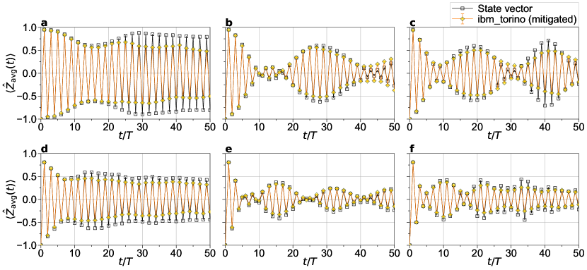
Figure S3: Enlarged plots of Fig. S2, focusing on the time evolution for up to 50 time steps.

To assess the accuracy of various tensor network methods, including matrix product state (MPS) [2] and two-dimensional tensor network state (2dTNS) methods (for details of our 2dTNS simulations, see Sec. S5), we compare the results of $\langle\hat{Z}_{\rm avg}(t)\rangle$ obtained by these methods with the numerically exact results calculated by the state-vector method in Figs. S4 and S5. As shown in Figs. S4a-c and S5a-c, when $\theta_{x}=0.9\pi$, $\langle\hat{Z}_{\rm avg}(t)\rangle$ obtained by these tensor network methods with relatively small bond dimensions $\chi$ (MPS with $\chi=300$ and 2dTNS with $\chi=40$) sufficiently converge consistently to the numerically exact values, even for time steps up to 100. However, as shown in Figs. S4d-f and S5d-f, when $\theta_{x}=0.8\pi$, which is close to the crossover boundary between the DTC/DTQC and thermalised regimes, a larger $\chi$ is required to obtain the converged value, due to the increase of entanglement. For example, when $(\theta_{x},\theta_{z})=(0.8\pi,0)$ (Fig. S5d), 2dTNS with $\chi=400$ is insufficient to obtain the numerically exact results for $t\gtrsim 50$. A similar trend is observed for other parameters shown in Figs. S5e,f and for the MPS method shown in Figs. S4d-f. These results suggest that the long-time time-evolution simulations of $\langle\hat{Z}_{\rm avg}(t)\rangle$ based on classical tensor network methods already face challenges even for $L=28$ in a parameter region around $\theta_{x}=0.8\pi$. We expect to encounter similar challenges for $L=133$, where the numerically exact state-vector method cannot be applied, although a recent report suggests that the accuracy of a 2dTNS method improves as the system size increases [3]. This emphasises the significance of utilising a quantum computer precisely in this parameter regime.

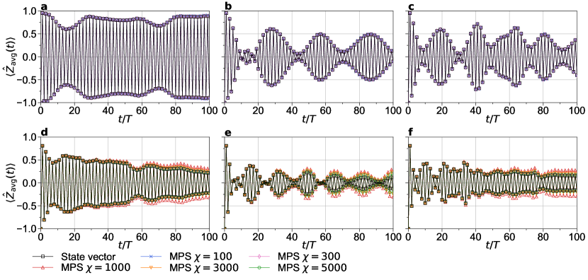
Figure S4: Comparison of the results for $\langle\hat{Z}_{\rm avg}(t)\rangle$ on the $L=28$ heavy-hexagonal lattice obtained by the MPS method with various bond dimensions ($\chi=100$, 300, 1000, 3000, and 5000) and the state-vector method. The parameters $(\theta_{x},\theta_{z})$ are a $(0.9\pi,0)$, b $(0.9\pi,0.5\pi)$, c $(0.9\pi,\pi)$, d $(0.8\pi,0)$, e $(0.8\pi,0.5\pi)$, and f $(0.8\pi,\pi)$.

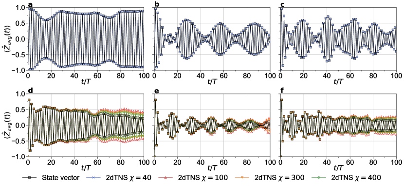
Figure S5: Comparison of the results for $\langle\hat{Z}_{\rm avg}(t)\rangle$ on the $L=28$ heavy-hexagonal lattice obtained by the 2dTNS method with various bond dimensions ($\chi=40$, 100, 300, and 400) and the state-vector method. The parameters $(\theta_{x},\theta_{z})$ are a $(0.9\pi,0)$, b $(0.9\pi,0.5\pi)$, c $(0.9\pi,\pi)$, d $(0.8\pi,0)$, e $(0.8\pi,0.5\pi)$, and f $(0.8\pi,\pi)$.

S3 Results for a heavy-hexagonal lattice of $L=133$ qubits

Figure S6 shows the error-unmitigated raw data of the average magnetisation $\langle\hat{Z}_{\rm avg}(t)\rangle_{0}$ for up to 100 time steps obtained for the $L=133$ system using ibm_torino (see Fig. 1a). Here, the average is performed over the same set $A$ of qubits as described in the main text, i.e., $A=\{57,58,59,60,61,62,63,64,65,66,67,68,69,70,71\}$. Remarkably, even without error mitigation, distinct signals of period-doubling oscillations persist for over 100 time steps. To mitigate errors in the raw data for $\theta_{x}\neq\pi$, the results corresponding to the trivial cases with $\theta_{x}=\pi$ are utilised, as explained in Eq. (4).

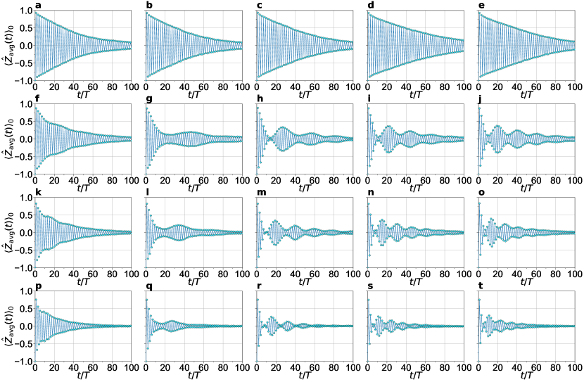
Figure S6: Error-unmitigated raw data $\langle\hat{Z}_{\rm avg}(t)\rangle_{0}$ for the heavy-hexagonal lattice of $L=133$ qubits obtained using ibm_torino (see Fig. 1a). The parameters $(\theta_{x},\theta_{z})$ are a $(\pi,0)$, b $(\pi,0.25\pi)$, c $(\pi,0.5\pi)$, d $(\pi,0.75\pi)$, e $(\pi,\pi)$, f $(0.9\pi,0)$, g $(0.9\pi,0.25\pi)$, h $(0.9\pi,0.5\pi)$, i $(0.9\pi,0.75\pi)$, j $(0.9\pi,\pi)$, k $(0.85\pi,0)$, l $(0.85\pi,0.25\pi)$, m $(0.85\pi,0.5\pi)$, n $(0.85\pi,0.75\pi)$, o $(0.85\pi,\pi)$, p $(0.8\pi,0)$, q $(0.8\pi,0.25\pi)$, r $(0.8\pi,0.5\pi)$, s $(0.8\pi,0.75\pi)$, and t $(0.8\pi,\pi)$.

For the trivial cases with $\theta_{x}=\pi$, as shown in Figs. S6a-e, $|\langle\hat{Z}_{\rm avg}(t)\rangle_{0}|$ should ideally be 1. However, deviations from this ideal value are observed, which become more pronounced with increasing time steps, owing to the noise and decoherence inherent in the quantum device. The number of CZ gates in the quantum circuit increases by 150 for each operation of $\hat{U}_{\text{F}}$ as defined in Eq. (2). At $t/T=100$, the quantum circuit volume $v=15000$ (defined by the total number of CZ gates) superficially implies $|\langle\hat{Z}_{\rm avg}(t=100T)\rangle_{0}|=(1-p)^{v}\simeq 10^{-27}$, with a typical two-qubit infidelity in ibm_torino of $p=4\times 10^{-3}$. However, in practice, we observe $|\langle\hat{Z}_{\rm avg}(t=100T)\rangle_{0}|\simeq 0.1$ in Figs. S6a-e, suggesting an effective quantum circuit volume $v_{\text{eff}}\simeq 600$. Since we measure local observables, $v_{\text{eff}}$ is significantly smaller than $v$, as discussed in Ref. [4]. Additionally, it is interesting to notice that the raw data for the $L=28$ system with the trivial parameters, as shown in Figs. S1a-c, also exhibit $|\langle\hat{Z}_{\rm avg}(t=100T)\rangle_{0}|\simeq 0.1-0.15$, indicating a similar $v_{\text{eff}}$.

In Fig. 2d of the main text, we demonstrated that the averaged magnetisation $\langle\hat{Z}_{\rm avg}(t)\rangle$ obtained from ibm_torino with the error mitigation agrees well with those of classical 2dTNS simulations at $(\theta_{x},\theta_{z})=(0.8\pi,0.5\pi)$ for the $L=133$ system over 50 time steps. In Figs. S7 and S8, we extend this comparison to other parameters over 100 time steps. As shown in Figs. S7a-c and S8a-c, when $\theta_{x}=0.9\pi$, the averaged magnetisation $\langle\hat{Z}_{\rm avg}(t)\rangle$ obtained by the 2dTNS method with a relatively small bond dimension $\chi=20$ already converges sufficiently. This implies that the 2dTNS results for these parameter sets are reliable even for up to 100 time steps. Indeed, this parameter region exhibits limited entanglement growth over time steps, as indicated by the agreement between the MPS results with relatively small bond dimensions and the 2dTNS results (see Figs. S9a-c and S10a-c). Moreover, it is particularly remarkable that despite the simple error mitigation protocol introduced in Eq. (4) of the main text, the error-mitigated $\langle\hat{Z}_{\rm avg}(t)\rangle$ obtained from ibm_torino are in relatively good alignment with the 2dTNS results (see Figs. S7a-c and S8a-c).

On the other hand, as shown in Figs. S7d-f and S8d-f, the convergence of the 2dTNS results for $\theta_{x}=0.8\pi$ is slow with increasing the bond dimension, especially for long time steps, as anticipated from the results for the $L=28$ system shown in Figs. S5d-f. This parameter region is close to the crossover boundary between the DTC/DTCQ and thermalised regimes, where extensive entanglement growth is expected. Due to the substantial increase in entanglement, the performance of tensor-network simulations is significantly degraded, resulting in a noticeable discrepancy between MPS and 2dTNS as shown in Figs. S9d-f and S10d-f. Although the classical 2dTNS simulations may not have yet converged in these parameter sets for $t\gtrsim 50$, we still observe that the error-mitigated $\langle\hat{Z}_{\rm avg}(t)\rangle$ obtained from ibm_torino align well with the 2dTNS results (see Figs. S7d-f and S8d-f). Given that this is the parameter region where classical simulations face challenges, it underscores the value of quantum computers precisely in this parameter region.

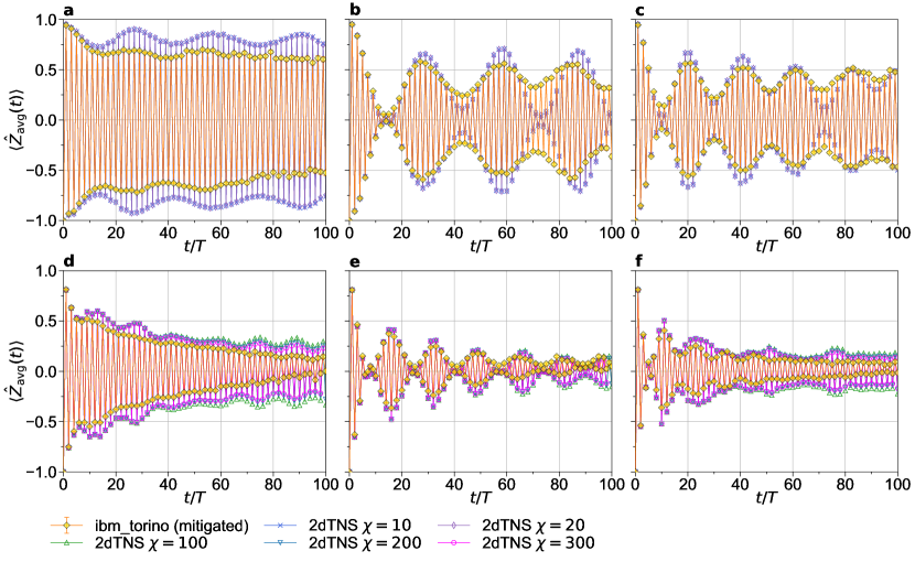
Figure S7: Error-mitigated data $\langle\hat{Z}_{\rm avg}(t)\rangle$ are compared with the results obtained by the 2dTNS method with various bond dimensions ($\chi=10$, 20, 100, 200, and 300) for the heavy-hexagonal lattice of $L=133$ qubits. The parameters $(\theta_{x},\theta_{z})$ are a $(0.9\pi,0)$, b $(0.9\pi,0.5\pi)$, c $(0.9\pi,\pi)$, d $(0.8\pi,0)$, e $(0.8\pi,0.5\pi)$, and f $(0.8\pi,\pi)$.

Figure S8: Enlarged plots of Fig. S7, focusing on the time evolution for up to 50 time steps.

Figure S9: Comparison of the results for $\langle\hat{Z}_{\rm avg}(t)\rangle$ on the heavy-hexagonal lattice of $L=133$ qubits obtained by the 2dTNS method with a given bond dimension ($\chi=20$ in panels a-c and 300 in panels d-f) and the MPS method with various bond dimensions ($\chi=1000$, 3000, and 5000). The parameters $(\theta_{x},\theta_{z})$ are a $(0.9\pi,0)$, b $(0.9\pi,0.5\pi)$, c $(0.9\pi,\pi)$, d $(0.8\pi,0)$, e $(0.8\pi,0.5\pi)$, and f $(0.8\pi,\pi)$.

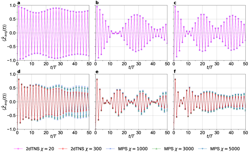
Figure S10: Enlarged plots of Fig. S9, focusing on the time evolution for up to 50 time steps.

In Figs. S11a-f, we show the spatial distribution of error-mitigated $\langle\hat{Z}_{j}(t)\rangle$ at $t/T=2$, 16, 24, 32, and 40 obtained using ibm_torino for the $L=133$ system with the parameter $(\theta_{x},\theta_{z})=(0.9\pi,0.5\pi)$. These results are compared with those obtained by the MPS method in Figs. S11g-l. Here, we initialise the state $|\psi(0)\rangle$ as a product state with all qubits set to $|0\rangle$, representing the fully polarised state. As shown in Fig. S12c, we also observe a longer-period oscillation in the averaged magnetisation $\langle\hat{Z}_{\rm avg}(t)\rangle$ upon introducing non-zero $\theta_{z}$, implying the emergence of a DTQC, despite the initial state differing from that used elsewhere in this study. Interestingly, the period of this oscillation closely resembles that observed in Fig. S7b, where the initial state is set differently. Furthermore, we find in Fig. S12c that the error-mitigated data are in good agreement with the results of MPS over 40-time steps.

Now, it is interesting to investigate the nature of the time-evolved state at characteristic times. As shown in Fig. S12c, the nodes of the longer-period oscillation occur at $t/T\simeq 14$ and slightly beyond $40$, which are similar to those observed in Fig. S8b. At times near these nodes, specifically $t/T=16$ and $40$ as shown in Figs. S11i and S11l, respectively, we observe that the time-evolved state $|\psi(t)\rangle$ exhibits a Neel-like structure in the MPS simulations. Even in ibm_torino, we observe, at least partially, a similar Neel-like structure, as shown in Figs. S11c and S11f. Conversely, at times near the antinodes, such as $t/T=2$, $24$, and $32$ shown in Figs. S11g, S11j, and S11k, respectively, the time-evolved state $|\psi(t)\rangle$ exhibits a ferromagnetic (FM)-like structure in the MPS simulations. Similarly, in ibm_torino, we observe a comparable FM-like structure, albeit partially, as shown in Figs. S11a, S11d, and S11e.

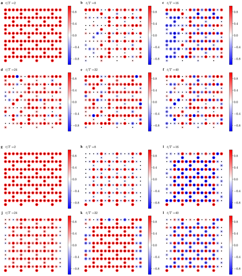
Figure S11: Time evolution of local expectation values $\langle Z_{j}(t)\rangle$ at $t/T=2$, 8, 16, 24, 32, and 40 on the heavy-hexagonal lattice of $L=133$ qubits with the parameter $(\theta_{x},\theta_{z})=(0.9\pi,0.5\pi)$. a-f Error-mitigated expectation values obtained using ibm_torino. g-l The corresponding results obtained by the MPS method with the bond dimension $\chi=1000$. Here, the initial state is prepared as a product state with all qubits set to $|0\rangle$, representing a fully-polarised state.

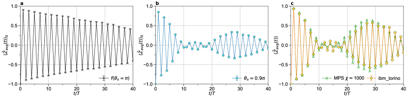
Figure S12: (a) Raw data of the averaged magnetisation $\langle\hat{Z}_{\rm avg}(t)\rangle_{0,\theta_{x}=\pi}$ for the heavy-hexagonal lattice of $L=133$ qubits with the parameter $(\theta_{x},\theta_{z})=(\pi,0.5\pi)$ obtained using ibm_torino. (b) Same as (a), but with the parameter $(\theta_{x},\theta_{z})=(0.9\pi,0.5\pi)$. (c) Error-mitigated data (yellow diamonds) of the averaged magnetisation $\langle\hat{Z}_{\rm avg}(t)\rangle$ for the heavy-hexagonal lattice of $L=133$ qubits with the parameter $(\theta_{x},\theta_{z})=(0.9\pi,0.5\pi)$. The results obtained by the MPS method with the bond dimension $\chi=1000$ are also shown with green triangles. Here, the initial state is prepared as a product state with all qubits set to $|0\rangle$, i.e., a fully-polarised state.

S4 Results for a one-dimensional lattice of $L=112$ qubits

While the emergence of a DTC in a one-dimensional system with short-range interactions necessitates many-body localisation, exploring the one-dimensional case driven by the same Floquet operator $\hat{U}_{\rm F}$ in Eq. (2) remains valuable. This investigation serves to highlight differences from the two-dimensional case examined throughout this paper and allows for further assessment of the reliability of results obtained using ibm_torino, along with the error-mitigation protocol introduced in Eq. (4).

A one-dimensional lattice of $L=112$ qubits can be incorporated into the heavy-hexagonal lattice geometry of the IBM Heron processor, ibm_torino, as depicted in Fig. S13. In this configuration, qubits constituting the one-dimensional lattice are interconnected by red and blue edges. The two-qubit $\hat{R}_{Z_{i}Z_{j}}(\theta_{J})$ gates in the single-cycle Floquet operator $\hat{U}_{\rm F}$ are applied on red or blue bonds concurrently in the quantum circuit. The initial state $|\psi(0)\rangle$ for the time evolution is prepared as a product state, forming a domain-wall configuration of $|0\rangle$’s and $|1\rangle$’s, represented by white and black circles, respectively, in Fig. S13. We evaluate the time evolution of the averaged magnetisation ${\hat{Z}_{\rm avg}}(t)$, defined in Eq. (3), over the same set $A$ of qubits as in the heavy-hexagonal lattice of $L=133$ qubits, i.e., $A=\{57,58,59,60,61,62,63,64,65,66,67,68,69,70,71\}$ (the qubit labels are indicated in Fig. S13).

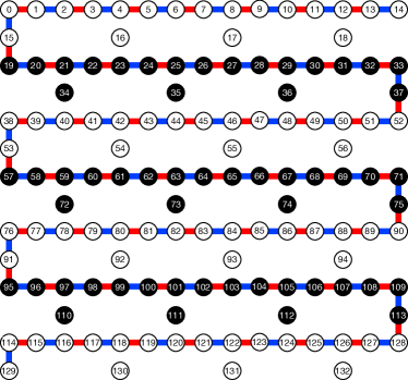
Figure S13: A one-dimensional lattice of $L=112$ qubits embedded in the heavy-hexagonal lattice geometry of the IBM Quantum Heron processor, ibm_torino. The qubits forming the one-dimensional lattice are connected by red and blue edges. When the quantum device is utilised, $\hat{R}_{Z_{i}Z_{j}}(\theta_{J})$ gates in the single-cycle Floquet operator $\hat{U}_{\rm F}$ applied on red or blue bonds are operated in parallel. The initial state is prepared as a product state with qubits indicated by white (black) circles set to $|0\rangle$ ($|1\rangle$).

Figures S14b and S14c show the error-unmitigated raw data $\langle\hat{Z}_{\rm avg}(t)\rangle_{0}$ obtained using ibm_torino for the one-dimensional system of $L=112$ qubits with the parameters $(\theta_{x},\theta_{z})=(0.9\pi,0.5\pi)$ and $(0.8\pi,0.5\pi)$, respectively. Additionally, Fig. S14a shows the error-unmitigated raw data $\langle\hat{Z}_{\rm avg}(t)\rangle_{0}$ for the same system but with $(\theta_{x},\theta_{z})=(\pi,0.5\pi)$, which are utilised to mitigate errors for $\langle\hat{Z}_{\rm avg}(t)\rangle_{0}$ with $(\theta_{x},\theta_{z})=(0.9\pi,0.5\pi)$ and $(0.8\pi,0.5\pi)$ shown in Figs. S14b and S14c. From the value of $|\langle\hat{Z}_{\rm avg}(t=80T)\rangle_{0}|$ shown in Fig. S14a, we can estimate the effective quantum circuit volume $v_{\rm eff}\simeq 350$ at $t/T=80$, which is significantly smaller than the quantum circuit volume $v=8880$ (the number of CZ gates in the quantum circuit increases by 111 for each operation of $\hat{U}_{\rm F}$ in the one-dimensional system).

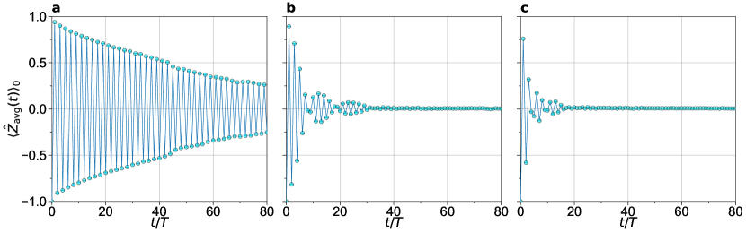
Figure S14: Error-unmitigated raw data $\langle\hat{Z}_{\rm avg}(t)\rangle_{0}$ for the one-dimensional lattice of $L=112$ qubits obtained using ibm_torino (see Fig. S13). The parameters $(\theta_{x},\theta_{z})$ are a $(\pi,0.5\pi)$, b $(0.9\pi,0.5\pi)$, and c $(0.8\pi,0.5\pi)$.

The error-mitigated data $\langle\hat{Z}_{\rm avg}(t)\rangle$ for the one-dimensional system of $L=112$ qubits with the parameters $(\theta_{x},\theta_{z})=(0.9\pi,0.5\pi)$ and $(0.8\pi,0.5\pi)$ are shown in Fig. S15. In sharp contrast to the case for the heavy-hexagonal lattice of $L=133$ qubits, the period-doubling oscillations observed in the one-dimensional system are much weaker against the deviation of $\theta_{x}$ from $\pi$. We find that the signals with these oscillations decay rather quickly in time steps for other parameter sets of $(\theta_{x},\theta_{z})$ in one dimension, even when $\theta_{z}=0.9$.

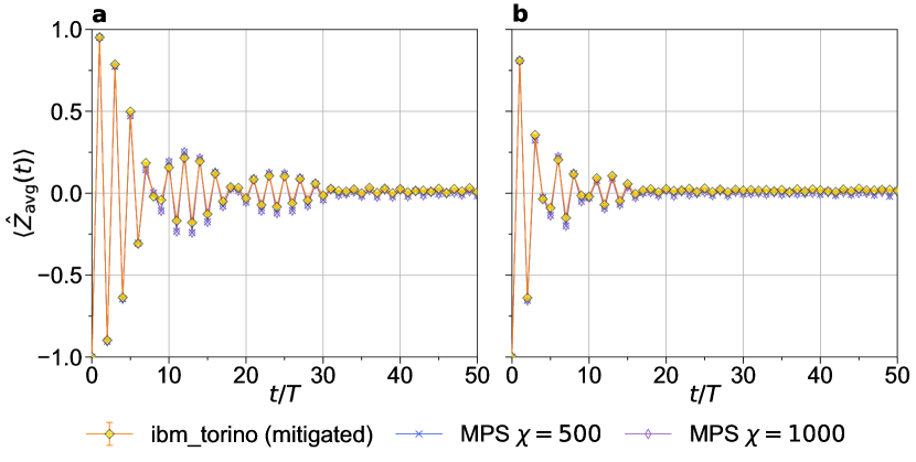
Figure S15: Error-mitigated data $\langle\hat{Z}_{\rm avg}(t)\rangle$ (yellow diamonds) are compared with the results obtained by the MPS simulations with the bond dimensions $\chi=500$ and 1000 (shown as blue crosses and purple diamonds, respectively) for the one-dimensional lattice of $L=112$ qubits. The parameters $(\theta_{x},\theta_{z})$ are (a) $(0.9\pi,0.5\pi)$ and (b) $(0.8\pi,0.5\pi)$.

Moreover, in Fig. S15, the results for $\langle\hat{Z}_{\rm avg}(t)\rangle$ obtained using ibm_torino are compared with those calculated by the MPS method with the bond dimensions $\chi=500$ and 1000, exhibiting the converged values. Remarkably, despite the simplicity of the error-mitigation protocol introduced, these two results obtained using ibm_torino and the MPS method show excellent agreement, confirming the reliability of the results obtained using ibm_torino.

S5 Tensor network simulations: 2dTNS

In this section, we describe our 2dTNS method based on a gauging tensor network technique. Gauging tensor network states (TNSs) provide a compact representation of quantum states within an approximation framework [5, 6, 7, 8, 9, 10, 11, 12, 13, 14, 3]. The gauging tensor network consists of two types of tensors: vertex tensors and gauge tensors. The vertex tensor has a physical bond representing qubit degrees of freedom, as well as virtual bonds that reflect the topology of the system. The gauge tensor is positioned on the edge connecting neighboring vertex tensors. The structure of the gauging tensor network for the IBM Quantum Heron processor, ibm_torino, which forms the heavy-hexagonal lattice, is illustrated in Fig. S16. For the heavy-hexagonal lattice, there are two types of vertex tensors: one with two virtual bonds and the other with three virtual bonds. The dimension of the virtual bond, i.e., bond dimension $\chi$, controls the accuracy of the approximation. In our study, $\chi$ denotes the maximum bond dimension utilised in a TNS.

Figure S16: Schematic structure of the two-dimensional gauging tensor network for the heavy-hexagonal lattice comprising $L=133$ qubits. Edges represent virtual bonds with bond dimension $\chi$. Vertex tensors, denoted as squares, have virtual bonds along with a physical bond representing qubit degrees of freedom. Gauge tensors, depicted as diamonds, are positioned on the edges connecting neighboring vertex tensors.

To apply a two-qubit gate to a gauging TNS with bond dimension $\chi$, we employ the time-evolving block decimation (TEBD) method Vidal03, outlined in Fig. S17. Initially, in step (a), the surrounding gauge tensors and the vertex tensors targeted for the two-qubit gate are contracted. Following this, QR decomposition is performed on the vertex tensor in step (b) to optimise the computational efficiency for the subsequent singular value decomposition (SVD) in step (d). All tensors connected to the two-qubit gate, along with the gauge tensor, are contracted in step (c). SVD is then executed on the resulting tensor in step (d), yielding a total of $2\chi$ singular values. To prevent an increase in bond dimension, only the $\chi$ largest singular values are retained, with the remaining space truncated to dimension $\chi$. Subsequently, this truncated diagonal matrix, composed of the $\chi$ largest singular values, replaces the original gauge tensor, with the neighboring vertex tensors updated, in steps (e)-(g).

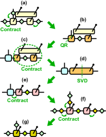
Figure S17: A depiction of the time-evolved block decimation (TEBD) process for a TNS given in Fig. S16. (a) The surrounding gauge tensors are absorbed into the vertex tensors to which a two-qubit gate is applied. (b) QR decomposition is performed on the vertex tensor which has the three virtual bonds to reduce the computational cost for the following singular value decomposition (SVD) procedure. (c) All tensors connected to the two-qubit gate and the gauge tensor between the two vertex tensors are contracted. (d) SVD is performed on the tensor obtained in step (c). (e) The isometric tensor obtained from the QR decomposition in step (b) is incorporated into the new tensor obtained by SVD in step (d). (f) Inverses of the surrounding gauge tensors are computed and absorbed into the vertex tensors which have the physical bonds. (g) New tensors are obtained.

More generally, in a gauging TNS, gauge tensors are typically represented as diagonal matrices. While a gauging TNS can describe the same quantum state, there exist various approaches to implement the gauge at an edge. One particularly notable gauge is the canonical gauge, also known as Vidal’s gauge. Within this framework of the Vidal gauge, the vertex tensors become isometric after absorbing all but one of the gauge tensors on their adjacent bonds, as schematically shown in Fig. S18(a). A notable advantage of employing the Vidal gauge is evident when computing the expectation value of a local physical quantity. For instance, when evaluating the expectation value of a physical quantity at a single site, the laborious task of contracting the entire tensor network is replaced with local tensor contraction, as shown in Fig. S18(c). This presents a significant advantage, particularly in the context of two-dimensional TNSs, where full contraction becomes computationally infeasible without resorting to approximate techniques.

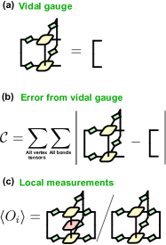
Figure S18: (a) A TNS in the Vidal gauge satisfies the isometric condition after absorbing all but one of their neighboring gauge tensors around the vertex tensors. (b) Deviation from the Vidal gauge is quantified with $\mathcal{C}$. Here, $\mathclose{\hbox{\set@color${|}$}\kern-1.38889pt\leavevmode\hbox{\set@color${|}$}}\mathcal{A}\mathclose{\hbox{\set@color${|}$}\kern-1.38889pt\leavevmode\hbox{\set@color${|}$}}$ represents the Frobenius norm for a tensor $\mathcal{A}$. Each tensor $\mathcal{A}$ after contraction is assumed to be normalised, i.e., $\tilde{\mathcal{A}}=\mathcal{A}/\mathclose{\hbox{\set@color${|}$}\kern-1.38889pt\leavevmode\hbox{\set@color${|}$}}\mathcal{A}\mathclose{\hbox{\set@color${|}$}\kern-1.38889pt\leavevmode\hbox{\set@color${|}$}}$. (c) Tensor contraction process for evaluating the expectation value $\langle\hat{O}_{i}\rangle$ of a local operator $\hat{O}_{i}$ (denoted as a red square), assuming that a TNS is in the Vidal gauge.

However, the TEBD process generally disrupts the Vidal gauge, even when we start with a TNS with the Vidal gauge. A procedure to restore this broken gauge is known as regauging. Particularly, simple and well-known regauging methods include trivial simple update (tSU) Jiang08,Corboz10,Jahromi19 and belief propagation Tindall23a,Tindall23b,Leifer08,Poulin08,Robeva18,Alkabetz21. In our study, we adopt the tSU regauging method outlined in Fig. S19. The tSU is a procedure essentially equivalent to that described in Fig. S17, except that the two-qubit gate is replaced with identity. Repeatedly applying this procedure across all edges in the tensor network improves the gauge and ultimately restores the Vidal gauge, in principle. While there is a mathematical proof for this in a tree tensor network [21], it is not established for a general tensor network with a loop structure. In our case, we assess the error $\mathcal{C}$ from the Vidal gauge, as defined in Fig. S18(b), at each time step, and iterate the tSU until it sufficiently converges. Moreover, we observe no significant difference between taking the Vidal gauge at every time step and only before measuring a physical quantity. This suggests that the accuracy of a TNS itself at each time step is not greatly influenced by whether the Vidal gauge is taken or not. Additionally, we performed calculations using the belief propagation Tindall23a,Tindall23b, and found that the results coincide with those obtained using the tSU, indicating convergence to the same fixed point Alkabetz21.

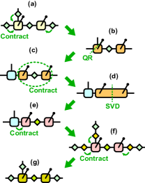
Figure S19: Procedure for the trivial simple update (tSU), essentially equivalent to the process outlined in Fig S17, but without the inclusion of the two-qubit gate.

We utilise this method, referred to as the 2dTNS method, to simulate the quantum dynamics governed by the Floquet operator $\hat{U}_{\rm F}$ described in the main text. Note that the single-qubit unitary gates $\hat{R}_{Z_{i}}(\theta_{z})$ and $\hat{R}_{X_{i}}(\theta_{x})$ can be treated exactly within this framework. As benchmark calculations, in Fig. S5, we compare the results of $\langle\hat{Z}_{\rm avg}(t)\rangle$ for the heavy-hexagonal lattice of $L=28$ qubits obtained by the 2dTNS method with various bond dimensions ($\chi=40$, 100, 300, and 400) with those obtained by the state-vector method.

Finally, Fig. S20 shows typical results for the convergence of a TNS towards that with the Vidal gauge when excuting the tSU regauging iterations during the simulations for the heavy-hexagonal lattice consisting of $L=133$ qubits, which corresponds to the results presented in Figs. S7 and S8. In this figure, each iteration of the tSU regauging process covers all the edges across the entire lattice. As the time step $t/T$ progresses, the number of iterations required for achieving a fixed accuracy also increases. Nevertheless, even at $t/T=100$, the convergence remains excellent with fewer than 30 iterations.

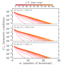
Figure S20: Convergence to the Vidal gauge vs. the number $m$ of iterations when employing the tSU regauging for the heavy-hexagonal lattice comprising $L=133$ qubits. The parameters $(\theta_{x},\theta_{z})$ are (a) $(0.8\pi,0)$, (b) $(0.8\pi,0.5\pi)$, and (c) $(0.8\pi,\pi)$. The bond dimension of the TNS is $\chi=200$. $C_{m}$ is the error from the Vidal gauge, defined as in Fig. S18(b), at iteration $m$, with color intensity denoting the time step $t/T$ (indicated at the top). We set the error tolerance of $10^{-8}$ to ensure compliance with the Vidal gauge in our simulations.

References

- Sacha and Zakrzewski [2017] K. Sacha and J. Zakrzewski, Time crystals: a review, Reports on Progress in Physics 81, 016401 (2017).
- Khemani et al. [2019] V. Khemani, R. Moessner, and S. L. Sondhi, A brief history of time crystals (2019), arXiv:1910.10745 [cond-mat.str-el] .
- Else et al. [2020] D. V. Else, C. Monroe, C. Nayak, and N. Y. Yao, Discrete time crystals, Annual Review of Condensed Matter Physics 11, 467–499 (2020).
- Guo and Liang [2020] L. Guo and P. Liang, Condensed matter physics in time crystals, New Journal of Physics 22, 075003 (2020).
- Zaletel et al. [2023] M. P. Zaletel, M. Lukin, C. Monroe, C. Nayak, F. Wilczek, and N. Y. Yao, Colloquium: Quantum and classical discrete time crystals, Rev. Mod. Phys. 95, 031001 (2023).
- Wilczek [2012] F. Wilczek, Quantum time crystals, Phys. Rev. Lett. 109, 160401 (2012).
- Bruno [2013a] P. Bruno, Impossibility of spontaneously rotating time crystals: A no-go theorem, Phys. Rev. Lett. 111, 070402 (2013a).
- Bruno [2013b] P. Bruno, Comment on “quantum time crystals”, Phys. Rev. Lett. 110, 118901 (2013b).
- Watanabe and Oshikawa [2015] H. Watanabe and M. Oshikawa, Absence of quantum time crystals, Phys. Rev. Lett. 114, 251603 (2015).
- Sacha [2015] K. Sacha, Modeling spontaneous breaking of time-translation symmetry, Phys. Rev. A 91, 033617 (2015).
- Else et al. [2016] D. V. Else, B. Bauer, and C. Nayak, Floquet time crystals, Phys. Rev. Lett. 117, 090402 (2016).
- Khemani et al. [2016] V. Khemani, A. Lazarides, R. Moessner, and S. L. Sondhi, Phase structure of driven quantum systems, Phys. Rev. Lett. 116, 250401 (2016).
- von Keyserlingk et al. [2016] C. W. von Keyserlingk, V. Khemani, and S. L. Sondhi, Absolute stability and spatiotemporal long-range order in floquet systems, Phys. Rev. B 94, 085112 (2016).
- Yao et al. [2017] N. Y. Yao, A. C. Potter, I.-D. Potirniche, and A. Vishwanath, Discrete time crystals: Rigidity, criticality, and realizations, Phys. Rev. Lett. 118, 030401 (2017).
- Zhang et al. [2017] J. Zhang, P. W. Hess, A. Kyprianidis, P. Becker, A. Lee, J. Smith, G. Pagano, I.-D. Potirniche, A. C. Potter, A. Vishwanath, N. Y. Yao, and C. Monroe, Observation of a discrete time crystal, Nature 543, 217–220 (2017).
- Ippoliti et al. [2021] M. Ippoliti, K. Kechedzhi, R. Moessner, S. Sondhi, and V. Khemani, Many-body physics in the nisq era: Quantum programming a discrete time crystal, PRX Quantum 2, 030346 (2021).
- Mi et al. [2022] X. Mi, M. Ippoliti, C. Quintana, A. Greene, Z. Chen, J. Gross, F. Arute, K. Arya, J. Atalaya, R. Babbush, J. C. Bardin, J. Basso, A. Bengtsson, A. Bilmes, A. Bourassa, L. Brill, M. Broughton, B. B. Buckley, D. A. Buell, B. Burkett, N. Bushnell, B. Chiaro, R. Collins, W. Courtney, D. Debroy, S. Demura, A. R. Derk, A. Dunsworth, D. Eppens, C. Erickson, E. Farhi, A. G. Fowler, B. Foxen, C. Gidney, M. Giustina, M. P. Harrigan, S. D. Harrington, J. Hilton, A. Ho, S. Hong, T. Huang, A. Huff, W. J. Huggins, L. B. Ioffe, S. V. Isakov, J. Iveland, E. Jeffrey, Z. Jiang, C. Jones, D. Kafri, T. Khattar, S. Kim, A. Kitaev, P. V. Klimov, A. N. Korotkov, F. Kostritsa, D. Landhuis, P. Laptev, J. Lee, K. Lee, A. Locharla, E. Lucero, O. Martin, J. R. McClean, T. McCourt, M. McEwen, K. C. Miao, M. Mohseni, S. Montazeri, W. Mruczkiewicz, O. Naaman, M. Neeley, C. Neill, M. Newman, M. Y. Niu, T. E. O’Brien, A. Opremcak, E. Ostby, B. Pato, A. Petukhov, N. C. Rubin, D. Sank, K. J. Satzinger, V. Shvarts, Y. Su, D. Strain, M. Szalay, M. D. Trevithick, B. Villalonga, T. White, Z. J. Yao, P. Yeh, J. Yoo, A. Zalcman, H. Neven, S. Boixo, V. Smelyanskiy, A. Megrant, J. Kelly, Y. Chen, S. L. Sondhi, R. Moessner, K. Kechedzhi, V. Khemani, and P. Roushan, Time-crystalline eigenstate order on a quantum processor, Nature 601, 531–536 (2022).
- Frey and Rachel [2022] P. Frey and S. Rachel, Realization of a discrete time crystal on 57 qubits of a quantum computer, Science Advances 8, eabm7652 (2022), https://www.science.org/doi/pdf/10.1126/sciadv.abm7652 .
- Xiang et al. [2024] L. Xiang, W. Jiang, Z. Bao, Z. Song, S. Xu, K. Wang, J. Chen, F. Jin, X. Zhu, Z. Zhu, F. Shen, N. Wang, C. Zhang, Y. Wu, Y. Zou, J. Zhong, Z. Cui, A. Zhang, Z. Tan, T. Li, Y. Gao, J. Deng, X. Zhang, H. Dong, P. Zhang, S. Jiang, W. Li, Z. Lu, Z.-Z. Sun, H. Li, Z. Wang, C. Song, Q. Guo, F. Liu, Z.-X. Gong, A. V. Gorshkov, N. Y. Yao, T. Iadecola, F. Machado, H. Wang, and D.-L. Deng, Long-lived topological time-crystalline order on a quantum processor (2024), arXiv:2401.04333 [quant-ph] .
- Else et al. [2017] D. V. Else, B. Bauer, and C. Nayak, Prethermal phases of matter protected by time-translation symmetry, Phys. Rev. X 7, 011026 (2017).
- Huang et al. [2018] B. Huang, Y.-H. Wu, and W. V. Liu, Clean floquet time crystals: Models and realizations in cold atoms, Phys. Rev. Lett. 120, 110603 (2018).
- Pizzi et al. [2019] A. Pizzi, J. Knolle, and A. Nunnenkamp, Period- discrete time crystals and quasicrystals with ultracold bosons, Phys. Rev. Lett. 123, 150601 (2019).
- Machado et al. [2020] F. Machado, D. V. Else, G. D. Kahanamoku-Meyer, C. Nayak, and N. Y. Yao, Long-range prethermal phases of nonequilibrium matter, Phys. Rev. X 10, 011043 (2020).
- Kyprianidis et al. [2021] A. Kyprianidis, F. Machado, W. Morong, P. Becker, K. S. Collins, D. V. Else, L. Feng, P. W. Hess, C. Nayak, G. Pagano, N. Y. Yao, and C. Monroe, Observation of a prethermal discrete time crystal, Science 372, 1192–1196 (2021).
- Pizzi et al. [2021] A. Pizzi, J. Knolle, and A. Nunnenkamp, Higher-order and fractional discrete time crystals in clean long-range interacting systems, Nature Communications 12, 10.1038/s41467-021-22583-5 (2021).
- Collura et al. [2022] M. Collura, A. De Luca, D. Rossini, and A. Lerose, Discrete time-crystalline response stabilized by domain-wall confinement, Phys. Rev. X 12, 031037 (2022).
- Santini et al. [2022] A. Santini, G. E. Santoro, and M. Collura, Clean two-dimensional floquet time crystal, Phys. Rev. B 106, 134301 (2022).
- Orús [2019] R. Orús, Tensor networks for complex quantum systems, Nature Reviews Physics 1, 538 (2019).
- Weimer et al. [2021] H. Weimer, A. Kshetrimayum, and R. Orús, Simulation methods for open quantum many-body systems, Rev. Mod. Phys. 93, 015008 (2021).
- Cirac et al. [2021] J. I. Cirac, D. Pérez-García, N. Schuch, and F. Verstraete, Matrix product states and projected entangled pair states: Concepts, symmetries, theorems, Rev. Mod. Phys. 93, 045003 (2021).
- Tindall et al. [2024] J. Tindall, M. Fishman, E. M. Stoudenmire, and D. Sels, Efficient tensor network simulation of ibm’s eagle kicked ising experiment, PRX Quantum 5, 010308 (2024).
- Chen et al. [2023] T. Chen, R. Shen, C. H. Lee, B. Yang, and R. W. Bomantara, A robust large-period discrete time crystal and its signature in a digital quantum computer (2023), arXiv:2309.11560 [quant-ph] .
- McKay et al. [2023] D. C. McKay, I. Hincks, E. J. Pritchett, M. Carroll, L. C. G. Govia, and S. T. Merkel, Benchmarking Quantum Processor Performance at Scale, arXiv e-prints , arXiv:2311.05933 (2023), arXiv:2311.05933 [quant-ph] .
- Viola et al. [1999] L. Viola, E. Knill, and S. Lloyd, Dynamical decoupling of open quantum systems, Phys. Rev. Lett. 82, 2417 (1999).
- Souza et al. [2012] A. M. Souza, G. A. Álvarez, and D. Suter, Robust dynamical decoupling, Philosophical Transactions of the Royal Society A: Mathematical, Physical and Engineering Sciences 370, 4748–4769 (2012).
- Temme et al. [2017] K. Temme, S. Bravyi, and J. M. Gambetta, Error mitigation for short-depth quantum circuits, Phys. Rev. Lett. 119, 180509 (2017).
- Li and Benjamin [2017] Y. Li and S. C. Benjamin, Efficient variational quantum simulator incorporating active error minimization, Phys. Rev. X 7, 021050 (2017).
- van den Berg et al. [2023] E. van den Berg, Z. K. Minev, A. Kandala, and K. Temme, Probabilistic error cancellation with sparse pauli–lindblad models on noisy quantum processors, Nature Physics 19, 1116–1121 (2023).
- Swingle and Yunger Halpern [2018] B. Swingle and N. Yunger Halpern, Resilience of scrambling measurements, Phys. Rev. A 97, 062113 (2018).
- Vovrosh et al. [2021] J. Vovrosh, K. E. Khosla, S. Greenaway, C. Self, M. S. Kim, and J. Knolle, Simple mitigation of global depolarizing errors in quantum simulations, Phys. Rev. E 104, 035309 (2021).
- Mi et al. [2021] X. Mi, P. Roushan, C. Quintana, S. Mandrà, J. Marshall, C. Neill, F. Arute, K. Arya, J. Atalaya, R. Babbush, J. C. Bardin, R. Barends, J. Basso, A. Bengtsson, S. Boixo, A. Bourassa, M. Broughton, B. B. Buckley, D. A. Buell, B. Burkett, N. Bushnell, Z. Chen, B. Chiaro, R. Collins, W. Courtney, S. Demura, A. R. Derk, A. Dunsworth, D. Eppens, C. Erickson, E. Farhi, A. G. Fowler, B. Foxen, C. Gidney, M. Giustina, J. A. Gross, M. P. Harrigan, S. D. Harrington, J. Hilton, A. Ho, S. Hong, T. Huang, W. J. Huggins, L. B. Ioffe, S. V. Isakov, E. Jeffrey, Z. Jiang, C. Jones, D. Kafri, J. Kelly, S. Kim, A. Kitaev, P. V. Klimov, A. N. Korotkov, F. Kostritsa, D. Landhuis, P. Laptev, E. Lucero, O. Martin, J. R. McClean, T. McCourt, M. McEwen, A. Megrant, K. C. Miao, M. Mohseni, S. Montazeri, W. Mruczkiewicz, J. Mutus, O. Naaman, M. Neeley, M. Newman, M. Y. Niu, T. E. O’Brien, A. Opremcak, E. Ostby, B. Pato, A. Petukhov, N. Redd, N. C. Rubin, D. Sank, K. J. Satzinger, V. Shvarts, D. Strain, M. Szalay, M. D. Trevithick, B. Villalonga, T. White, Z. J. Yao, P. Yeh, A. Zalcman, H. Neven, I. Aleiner, K. Kechedzhi, V. Smelyanskiy, and Y. Chen, Information scrambling in quantum circuits, Science 374, 1479–1483 (2021).
- Kim et al. [2023] Y. Kim, A. Eddins, S. Anand, K. X. Wei, E. van den Berg, S. Rosenblatt, H. Nayfeh, Y. Wu, M. Zaletel, K. Temme, and A. Kandala, Evidence for the utility of quantum computing before fault tolerance, Nature 618, 500 (2023).
- Zener [1934] C. Zener, A theory of the electrical breakdown of solid dielectrics, Proc. R. Soc. Lond. A 145, 523 (1934).
- Verdel et al. [2020] R. Verdel, F. Liu, S. Whitsitt, A. V. Gorshkov, and M. Heyl, Real-time dynamics of string breaking in quantum spin chains, Phys. Rev. B 102, 014308 (2020).
- [45] GraceQ/tensor, https://github.com/gracequantum/tensor.

References

- [1] K. Seki and S. Yunoki, Spatial, spin, and charge symmetry projections for a fermi-hubbard model on a quantum computer, Phys. Rev. A 105, 032419 (2022).
- [2] R.-Y. Sun, T. Shirakawa, and S. Yunoki, Improved real-space parallelizable matrix-product state compression and its application to unitary quantum dynamics simulation, arXiv e-prints arXiv:2312.02667 (2023).
- [3] J. Tindall, M. Fishman, E. M. Stoudenmire, and D. Sels, Efficient tensor network simulation of ibm’s eagle kicked ising experiment, PRX Quantum 5, 010308 (2024).
- [4] K. Kechedzhi, S. Isakov, S. Mandrà, B. Villalonga, X. Mi, S. Boixo, and V. Smelyanskiy, Effective quantum volume, fidelity and computational cost of noisy quantum processing experiments, Future Generation Computer Systems 153, 431 (2024).
- [5] G. Vidal, Efficient classical simulation of slightly entangled quantum computations, Phys. Rev. Lett. 91, 147902 (2003).
- [6] G. Vidal, Efficient simulation of one-dimensional quantum many-body systems, Phys. Rev. Lett. 93, 040502 (2004).
- [7] Y.-Y. Shi, L.-M. Duan, and G. Vidal, Classical simulation of quantum many-body systems with a tree tensor network, Phys. Rev. A 74, 022320 (2006).
- [8] G. Vidal, Classical simulation of infinite-size quantum lattice systems in one spatial dimension, Phys. Rev. Lett. 98, 070201 (2007).
- [9] R. Orús and G. Vidal, Infinite time-evolving block decimation algorithm beyond unitary evolution, Phys. Rev. B 78, 155117 (2008).
- [10] D. Nagaj, E. Farhi, J. Goldstone, P. Shor, and I. Sylvester, Quantum transverse-field ising model on an infinite tree from matrix product states, Phys. Rev. B 77, 214431 (2008).
- [11] H. Kalis, D. Klagges, R. Orús, and K. P. Schmidt, Fate of the cluster state on the square lattice in a magnetic field, Phys. Rev. A 86, 022317 (2012).
- [12] S.-J. Ran, W. Li, B. Xi, Z. Zhang, and G. Su, Optimized decimation of tensor networks with super-orthogonalization for two-dimensional quantum lattice models, Phys. Rev. B 86, 134429 (2012).
- [13] H. N. Phien, I. P. McCulloch, and G. Vidal, Fast convergence of imaginary time evolution tensor network algorithms by recycling the environment, Phys. Rev. B 91, 115137 (2015).
- [14] J. Tindall and M. Fishman, Gauging tensor networks with belief propagation, SciPost Phys. 15, 222 (2023).
- [15] H. C. Jiang, Z. Y. Weng, and T. Xiang, Accurate determination of tensor network state of quantum lattice models in two dimensions, Phys. Rev. Lett. 101, 090603 (2008).
- [16] P. Corboz, R. Orús, B. Bauer, and G. Vidal, Simulation of strongly correlated fermions in two spatial dimensions with fermionic projected entangled-pair states, Phys. Rev. B 81, 165104 (2010).
- [17] S. S. Jahromi and R. Orús, Universal tensor-network algorithm for any infinite lattice, Phys. Rev. B 99, 195105 (2019).
- [18] M. Leifer and D. Poulin, Quantum graphical models and belief propagation, Annals of Physics 323, 1899 (2008).
- [19] D. Poulin and E. Bilgin, Belief propagation algorithm for computing correlation functions in finite-temperature quantum many-body systems on loopy graphs, Phys. Rev. A 77, 052318 (2008).
- [20] E. Robeva and A. Seigal, Duality of graphical models and tensor networks, Information and Inference: A Journal of the IMA 8, 273 (2018).
- [21] R. Alkabetz and I. Arad, Tensor networks contraction and the belief propagation algorithm, Phys. Rev. Res. 3, 023073 (2021).