An alternative measure for quantifying the heterogeneity in meta-analysis

Abstract

Quantifying the heterogeneity is an important issue in meta-analysis, and among the existing measures, the $I^{2}$ statistic is most commonly used. In this paper, we first illustrate with a simple example that the $I^{2}$ statistic is heavily dependent on the study sample sizes, mainly because it is used to quantify the heterogeneity between the observed effect sizes. To reduce the influence of sample sizes, we introduce an alternative measure that aims to directly measure the heterogeneity between the study populations involved in the meta-analysis. We further propose a new estimator, namely the $I^{2}_{\rm A}$ statistic, to estimate the newly defined measure of heterogeneity. For practical implementation, the exact formulas of the $I^{2}_{\rm A}$ statistic are also derived under two common scenarios with the effect size as the mean difference (MD) or the standardized mean difference (SMD). Simulations and real data analysis demonstrate that the $I^{2}_{\rm A}$ statistic provides an asymptotically unbiased estimator for the absolute heterogeneity between the study populations, and it is also independent of the study sample sizes as expected. To conclude, our newly defined $I_{A}^{2}$ statistic can be used as a supplemental measure of heterogeneity to monitor the situations where the study effect sizes are indeed similar with little biological difference. In such scenario, the fixed-effect model can be appropriate; nevertheless, when the sample sizes are sufficiently large, the $I^{2}$ statistic may still increase to 1 and subsequently suggest the random-effects model for meta-analysis.

$Key\ words$: ANOVA, heterogeneity, intraclass correlation coefficient, meta-analysis, the $I^{2}$ statistic, the $I^{2}_{\rm A}$ statistic

1 Introduction

Meta-analysis is a statistical technique for evidence-based practice, which aims to synthesize multiple studies and produce a summary conclusion for the whole body of research (Egger and Smith,, 1997). In the literature, there are two commonly used statistical models for meta-analysis, namely, the fixed-effect model and the random-effects model. Among them, the fixed-effect model assumes that the effect sizes of different studies are all the same, which is somewhat restrictive and may not be realistic in practice. The effect sizes often differ between the studies due to variability in study design, outcome measurement tools, risk of bias, and the participants, interventions and outcomes studied (Higgins et al.,, 2019), etc. Such diversity in the effect sizes is known as the heterogeneity. When the heterogeneity exists, the random-effects model ought to be applied for meta-analysis. In such scenarios, it is of great importance to properly quantify the heterogeneity so as to explore the generalizability of the findings from a meta-analysis.

To describe the heterogeneity in detail, we first introduce the random-effects model for meta-analysis. Let $k$ be the total number of studies, and $y_{i}$ be the observed effect sizes from the studies $i=1,\dots,k$. For each study with true effect size $\mu_{i}$, we assume that $y_{i}$ is normally distributed with mean $\mu_{i}=E(y_{i}|\mu_{i})$ and variance $\sigma_{y_{i}}^{2}={\rm var}(y_{i}|\mu_{i})$. Moreover, to account for the heterogeneity between the studies, we also assume that the individual effect sizes $\mu_{i}$ follow another normal distribution with mean $\mu$ and variance $\tau^{2}>0$. Taken together, the random-effects model for meta-analysis can be expressed as

$$y_{i}=\mu+\delta_{i}+\epsilon_{i},\quad\delta_{i}\stackrel{{\scriptstyle\text{i.i.d.}}}{{\sim}}N(0,\tau^{2}),\quad\epsilon_{i}\stackrel{{\scriptstyle\text{ind}}}{{\sim}}N(0,\sigma_{y_{i}}^{2}),$$ (1)

where “i.i.d.” represents independent and identically distributed, “ind” represents independently distributed, $\tau^{2}$ is the between-study variance, and $\sigma_{y_{i}}^{2}$ are the within-study variances. In addition, the study deviations $\delta_{i}=\mu_{i}-\mu$ and the random errors $\epsilon_{i}$ are assumed to be independent of each other. When $\delta_{i}$ are all zero, model (1) reduces to the fixed-effect model and there is no heterogeneity between the studies.

To test the existence of heterogeneity for model (1), Cochran, (1954) proposed the $Q$ statistic as $Q=\sum_{i=1}^{k}w_{i}(y_{i}-\sum_{i=1}^{k}w_{i}y_{i}/\sum_{i=1}^{k}w_{i})^{2}$, where $w_{i}=1/\sigma_{y_{i}}^{2}$ are the inverse-variance weights. Noting that $\sigma_{y_{i}}^{2}$ can often be estimated with high precision, it is a common practice in meta-analysis that the within-study variances are regarded as known. Nevertheless, when used as a measure of heterogeneity, it is often criticized that the value of $Q$ will increase with the number of studies. Another measure for heterogeneity is to apply the between-study variance $\tau^{2}$, yet it is known to be specific to a particular effect metric, making it impossible to compare across different meta-analyses (DerSimonian and Laird,, 1986). To have a fair comparison, Higgins and Thompson, (2002) and Higgins et al., (2003) introduced the $I^{2}$ statistic by a two-step procedure, under the assumption that the within-study variances $\sigma_{y_{i}}^{2}=\sigma_{y}^{2}$ are all the same. They first defined the measure of heterogeneity between the studies as

$${\rm ICC}_{\rm HT}=\frac{\tau^{2}}{{\rm var}(y_{i})}=\frac{\tau^{2}}{\tau^{2}+\sigma_{y}^{2}},$$ (2)

and then proposed

$$I^{2}=\frac{\hat{\tau}^{2}}{\hat{\tau}^{2}+\hat{\sigma}_{y}^{2}}=\max\left\{\frac{Q-(k-1)}{Q},0\right\}$$ (3)

to estimate the unknown ${\rm ICC}_{\rm HT}$, where $\hat{\tau}^{2}={\mbox{max}}\{\{Q-(k-1)\}/(\sum_{i=1}^{k}w_{i}-\sum_{i=1}^{k}w_{i}^{2}/\sum_{i=1}^{k}w_{i}),0\}$ is the Dersimonian-Laird estimator (DerSimonian and Laird,, 1986) and $\hat{\sigma}_{y}^{2}=\sum_{i=1}^{k}w_{i}(k-1)/\{(\sum_{i=1}^{k}w_{i})^{2}-\sum_{i=1}^{k}w_{i}^{2}\}$. When the within-study variances are all the same, $\hat{\sigma}_{y}^{2}$ is an estimate for the common $\sigma_{y}^{2}$. Otherwise if they differ, Böhning et al., (2017) has showed that $\hat{\sigma}_{y}^{2}$ is asymptotically identical to the harmonic mean $(\sum_{i=1}^{k}w_{i}/k)^{-1}$ of the within-study variances. Moreover, the $I^{2}$ statistic is also guaranteed to be within the interval $[0,1)$, which is appealing in that it does not depend on the number of studies and is irrespective of the effect metric.

Thanks to its nice properties, the $I^{2}$ statistic is nowadays routinely reported in the forest plots for meta-analyses, and/or used as a criterion for model selection between the fixed-effect model and the random-effects model. In Google Scholar, as of March 2024, the two papers by Higgins and Thompson, (2002) and Higgins et al., (2003) have been cited more than 30,000 and 52,000 times, respectively. Despite of its huge popularity, there were evidences in the literature reporting the limitations of the $I^{2}$ statistic. In particular, Rücker et al., (2008) found that the $I^{2}$ statistic always increases rapidly to 1 when the sample sizes are large, regardless of whether or not the heterogeneity between the studies is clinically important. For other discussions on the $I^{2}$ statistic as a measure of heterogeneity, one may refer to, for example, Riley et al., (2016), IntHout et al., (2016), Borenstein et al., (2017), Sangnawakij et al., (2019), Holling et al., (2020), and the references therein. This motivates us to further explore the characteristics of the $I^{2}$ statistic as a measure of heterogeneity for meta-analysis.

To answer this question, we first present a motivating example to demonstrate that the $I^{2}$ statistic was defined to quantify the heterogeneity between the observed effect sizes rather than that between the study populations. In view of this, we regard the $I^{2}$ statistic as a relative measure of heterogeneity. We further draw a connection between the one-way analysis of variance (ANOVA) and the random-effects meta-analysis, and subsequently introduce an alternative measure for quantifying the heterogeneity in the random-effects model, which is independent of study sample sizes and can serve as an absolute measure of heterogeneity. For details, see Section 3.2 for the defined ${\rm ICC}_{\rm MA}$ in formula (7). To move forward, the statistical properties of ${\rm ICC}_{\rm MA}$ are also derived to explore the distinction between our new measure and the existing measures including ${\rm ICC}_{\rm HT}$. Lastly, we propose an asymptotically unbiased estimator of the unknown ${\rm ICC}_{\rm MA}$, referred to as the $I^{2}_{\rm A}$ statistic, and show by simulations and real data analysis that it is independent of the study sample sizes.

The remainder of the paper is organized as follows. In Section 2, we give a motivating example to illustrate that ${\rm ICC}_{\rm HT}$ heavily depends on the study sample sizes. In Section Section 3, by drawing a close connection between ANOVA and the random-effects meta-analysis, we introduce an alternative measure for quantifying the heterogeneity between the studies. In Section 4, we derive the $I^{2}_{\rm A}$ statistic as an asymptotically unbiased estimator for the newly proposed absolute measure of heterogeneity. In Sections 5 and 6, we provide the detailed formulas of the $I^{2}_{\rm A}$ statistic for two common scenarios with the mean difference or the standardized mean difference as the effect size. While for practical implementation, real data analysis and numerical results are also presented for each scenario. Finally, we conclude the paper in Section 7 and provide the technical details in the Appendix.

2 A motivating example

In this section, we illustrate how ${\rm ICC}_{\rm HT}$ in (2) varies along with the sample sizes, and so may not be able to serve as a measure of heterogeneity between the study populations. To confirm this claim, we first consider a motivating example of three studies with data generated from normal populations $N(-0.05,1)$, $N(0,1)$ and $N(0.05,1)$, respectively. From the top-left panel of Figure 1, it is evident that the three study populations are largely overlapped. Taken the three study means as a random sample, the between-study variance can be estimated by the sample variance as $\tilde{\tau}^{2}=\{(-0.05-0)^{2}+(0-0)^{2}+(0.05-0)^{2}\}/2=0.0025$.

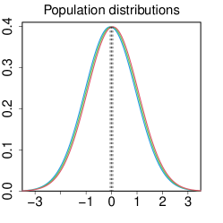
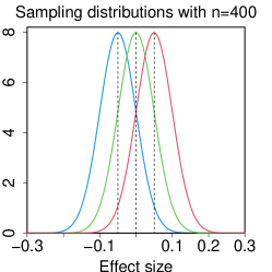
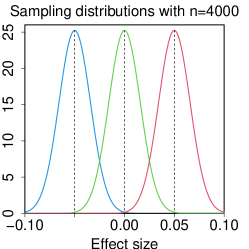
Figure 1: Population distributions of the three studies and the sampling distributions of the observed effect sizes. Left panel: Population distributions are $N(-0.05,1)$ in blue, $N(0,1)$ in green and $N(0.05,1)$ in red, respectively. Middle panel: Sampling distributions are $N(-0.05,0.0025)$, $N(0,0.0025)$ and $N(0.05,0.0025)$, respectively. Right panel: Sampling distributions are $N(-0.05,0.00025)$, $N(0,0.00025)$ and $N(0.05,0.00025)$, respectively.

To explain why ${\rm ICC}_{\rm HT}$ is not a measure of heterogeneity between the study populations, we consider two scenarios to meta-analyze the three studies, with the population means being treated as the effect sizes. The first scenario assumes $n=400$ patients in each study. By taking the sample means, the sampling distributions of the observed effect sizes are thus $N(-0.05,0.0025)$, $N(0,0.0025)$ and $N(0.05,0.0025)$, respectively, yielding $\sigma_{y}^{2}=0.0025$ as the common within-study variance. Further by the definition in (2), we have

$${\rm ICC}_{\rm HT}\approx\frac{0.0025}{0.0025+0.0025}=50\%.$$

In the second scenario, we consider $n=4000$ for each study. This leads to the sampling distributions of the observed effect sizes as $N(-0.05,0.00025)$, $N(0,0.00025)$ and $N(0.05,0.00025)$, respectively. Further by $\sigma_{y}^{2}=0.00025$, the measure of heterogeneity is

$${\rm ICC}_{\rm HT}\approx\frac{0.00025}{0.00025+0.0025}=90.9\%.$$

Finally, for ease of comparison, we also plot the sampling distributions of the observed effect sizes in Figure 1 for the two hypothetical scenarios with varying study sample sizes.

The above example clearly shows that ${\rm ICC}_{\rm HT}$, defined in (2) by Higgins and Thompson (2002), measures the heterogeneity between the observed effect sizes and thus heavily depends on the study sample sizes. In other words, ${\rm ICC}_{\rm HT}$ is a relative measure of heterogeneity for meta-analysis. Consequently, as a sample estimate of ${\rm ICC}_{\rm HT}$, the $I^{2}$ statistic is also heavily dependent on the sample sizes. This coincides with the observations by Rücker et al., (2008). Specifically, in our motivating example, ${\rm ICC}_{\rm HT}$ increases rapidly to about $90\%$ when the sample sizes are 4000, even though it is evident that the three populations are largely overlapped with each other. To summarize, when the study sample sizes $n_{i}$ are large enough, it will always yield an $I^{2}$ value being close to 1. On the other hand, compared with the population variance 1, the differences between the three study means $(-0.05,0,0.05)$ may not be clinically important. To support this claim, we note that the Scientific Committee of the European Food Safety Authority have also emphasized the importance of assessing the biological differences (EFSA Scientific Committee,, 2011). This hence motivates us to introduce an alternative measure that quantifies the heterogeneity between the study populations directly, in a way to reduce the influence of sample sizes.

3 A new measure of heterogeneity

To further explore the characteristics of ${\rm ICC}_{\rm HT}$, we also draw in this section an interesting connection between one-way analysis of variance (ANOVA) and meta-analysis. And on basis of that, a new measure for quantifying the heterogeneity between the study populations will be introduced, and moreover by studying its statistical properties, it is also explained why it can add new value to meta-analysis.

3.1 Connection between ANOVA and meta-analysis

To introduce the one-way ANOVA, we let $y_{ij}$ be the $j$th observation in the $i$th population, $i=1,\dots,k$ and $j=1,\dots,n_{i}$, where $k$ is the number of studies and $n_{i}$ are the study sample sizes from each population. The random-effects ANOVA for the observed data is then

$$y_{ij}=\mu+\delta_{i}+\xi_{ij},\quad\delta_{i}\stackrel{{\scriptstyle\text{i.i.d.}}}{{\sim}}N(0,\tau^{2}),\quad\xi_{ij}\stackrel{{\scriptstyle\text{i.i.d.}}}{{\sim}}N(0,\sigma^{2}),$$ (4)

where $\mu$ is the grand mean, $\delta_{i}$ are the treatment effects, and $\xi_{ij}$ are the random errors. We further assume that $\delta_{i}$ are i.i.d. normal random variables with mean 0 and variance $\tau^{2}\geq 0$, $\xi_{ij}$ are i.i.d. normal random errors with mean 0 and variance $\sigma^{2}>0$, and that $\delta_{i}$ and $\xi_{ij}$ are independent of each other. In addition, we refer to $\mu_{i}=\mu+\delta_{i}$ as the individual means, $\tau^{2}$ as the between-study variance, $\sigma^{2}$ as the common error variance for all $k$ populations, and $\tau^{2}+\sigma^{2}$ as the total variance of each observation.

To draw a close connection between ANOVA and meta-analysis, we consider a hypothetical scenario in which the experimenter first computed the sample mean and its variance for each population, namely $y_{i}=\sum_{j=1}^{n_{i}}y_{ij}/n_{i}$ and $\hat{\sigma}_{y_{i}}^{2}=\sum_{j=1}^{n_{i}}(y_{ij}-y_{i})^{2}/\{n_{i}(n_{i}-1)\}$ for $i=1,\dots,k$, and then reported these summary data rather than the raw data to the public. In practice, there are reasons why one must do so, including, for example, due to the privacy protection for which the individual patient data cannot be released. Under such a scenario, if some researchers want to re-analyze the experiment using only the publicly available data, it then yields a new random-effects model as

$$y_{i}=\mu+\delta_{i}+\epsilon_{i},\quad\delta_{i}\stackrel{{\scriptstyle\text{i.i.d.}}}{{\sim}}N(0,\tau^{2}),\quad\epsilon_{i}\stackrel{{\scriptstyle\text{ind}}}{{\sim}}N(0,\sigma^{2}/n_{i}),$$ (5)

where $y_{i}$ are the sample means, $\mu$ and $\delta_{i}$ are the same as defined in model (4), and $\epsilon_{i}=\sum_{j=1}^{n_{i}}\xi_{ij}/n_{i}$ are independent random errors with mean 0 and variance $\sigma^{2}/n_{i}$, where $i=1,\dots,k$. Now from the point of view of meta-analysis, if we treat $y_{i}$ as the reported effect sizes and $\hat{\sigma}^{2}_{y_{i}}$ as the within-study variances representing $\sigma^{2}/n_{i}$, then model (5) is essentially the same as the random-effects model in (1). This interesting connection shows that, when the ANOVA model with raw data only releases the summary data to the public, it will then yield a meta-analysis model with summary data.

Table 1: Connection between the ANOVA model in (4) and the meta-analysis model in (5), where $y_{i}=\sum_{j=1}^{n_{i}}y_{ij}/n_{i}$ and $\epsilon_{i}=\sum_{j=1}^{n_{i}}\xi_{ij}/n_{i}$ for $i=1,\dots,k$ and $j=1,\dots,n_{i}$.

	ANOVA	Meta-analysis
Model	$y_{ij}=\mu+\delta_{i}+\xi_{ij}$	$y_{i}=\mu+\delta_{i}+\epsilon_{i}$
Between-study variance	$\tau^{2}$	$\tau^{2}$
Error (or within-study) variance	$\sigma^{2}$	$\sigma^{2}/n_{i}$
Total variance	${\rm var}(y_{ij})=\tau^{2}+\sigma^{2}$	${\rm var}(y_{i})=\tau^{2}+\sigma^{2}/n_{i}$

For ease of comparison, we also summarize some key components in Table 1 for both the ANOVA model in (4) and the meta-analysis model in (5). For the meta-analysis model, under the assumption that the within-study variances, i.e. $\sigma^{2}/n_{i}$, are all equal, Higgins and Thompson, (2002) interpreted the measure of heterogeneity as the proportion of total variance that is “between studies”. More specifically, by the last column of Table 1, they introduced the measure of heterogeneity for meta-analysis as in (2), where $\sigma_{y}^{2}=\sigma^{2}/n_{i}$ is the common within-study variance for the observed effect sizes. This clearly explains why ${\rm ICC}_{\rm HT}$ will be heavily dependent on the study sample sizes. When the sample sizes go to infinity, the within-study variances will converge to zero so that ${\rm ICC}_{\rm HT}$ will increase to 1, as having been observed in Rücker et al., (2008). This also coincides with our motivating example in Section 2 that, when the sample size varies from 400 to 4000, their measure of heterogeneity will increase from $50\%$ to about $90\%$, regardless of whether or not the heterogeneity between the studies is clinically important.

For the ANOVA model, it is well known that the intraclass correlation coefficient (ICC) is the most commonly used measure of heterogeneity (Fisher,, 1925; Smith,, 1957; Donner,, 1979; McGraw and Wong,, 1996), which interprets the proportion of total variance that is “between populations”. More specifically, by Table 1, ${\rm ICC}$ can be expressed as

$${\rm ICC}=\frac{\tau^{2}}{{\rm var}(y_{ij})}=\frac{\tau^{2}}{\tau^{2}+\sigma^{2}}.$$ (6)

As shown in the hypothetical scenario, the ANOVA model in (4) and the meta-analysis model in (5) are, in fact, modeling the same populations, even though one uses the raw data and the other uses the summary data. In the special case when the mean value is taken as the effect size, it is known that the sample mean is a sufficient and complete statistic for the normal mean; in other words, the raw data and the summary data contain exactly the same information regarding the effect size. With this insight, we expect that the measures of heterogeneity between the study populations for the two models should also be the same, regardless of whether the raw data or the summary data are being used.

3.2 An intrinsic measure of heterogeneity

Inspired by the intrinsic connection between ANOVA and meta-analysis, we now follow the same assumption as in ANOVA that the population variances $n_{i}\sigma_{y_{i}}^{2}$ are all equal. For ease of presentation, we also denote the common study population variance as $\sigma_{\rm pop}^{2}$. Then by following ICC in (6) for ANOVA, we propose the following measure of heterogeneity for meta-analysis:

$${\rm ICC}_{\rm MA}=\frac{\tau^{2}}{{\rm var}(y_{ij})}=\frac{\tau^{2}}{\tau^{2}+\sigma_{\rm pop}^{2}}.$$ (7)

Note that the range of ${\rm ICC}_{\rm MA}$ is always within the interval $[0,1)$. Regarding the rationale of ${\rm ICC}_{\rm MA}$ for meta-analysis, one may also refer to the proposed measure in Sangnawakij et al., (2019).

To further study the properties of ${\rm ICC}_{\rm MA}$ and explain why it can serve as an absolute measure of heterogeneity for meta-analysis, we first present the three statistical properties of ${\rm ICC}_{\rm HT}$ as follows.

1. Monotonicity. ${\rm ICC}_{\rm HT}$ is a monotonically increasing function of the ratio $\tau^{2}/\sigma_{y}^{2}$. When the common within-study variance $\sigma_{y}^{2}$ is fixed, ${\rm ICC}_{\rm HT}$ will solely increase with the between-study variance $\tau^{2}$. This property was referred to as the “dependence on the extent of heterogeneity” by Higgins and Thompson, (2002).

2. Location and scale invariance. ${\rm ICC}_{\rm HT}$ is not affected by the location and scale of the effect sizes. This property was referred to as the “scale invariance” by Higgins and Thompson, (2002).

3. Study size invariance. ${\rm ICC}_{\rm HT}$ is not affected by the total number of studies $k$. This property was referred to as the “size invariance” by Higgins and Thompson, (2002).

Thanks to the above properties, the $I^{2}$ statistic is nowadays the most popular measure for quantifying the heterogeneity in meta-analysis, compared to other existing measures including $Q$ and $\tau^{2}$. Nevertheless, we do wish to point out that the “size invariance” in their property (iii) only represents the study size invariance but not includes the sample size invariance. As shown in the motivating example and also from the historical evidence in the literature, ${\rm ICC}_{\rm HT}$ does suffer from a heavy dependence on the study sample sizes.

While for the new measure of heterogeneity in (7), we show in Appendix A that ${\rm ICC}_{\rm MA}$ shares the following four properties:

1. Monotonicity. ${\rm ICC}_{\rm MA}$ is a monotonically increasing function of the ratio $\tau^{2}/\sigma_{\rm pop}^{2}$. When the common population variance $\sigma_{\rm pop}^{2}$ is fixed, ${\rm ICC}_{\rm MA}$ will solely increase with the between-study variance $\tau^{2}$.

2. Location and scale invariance. ${\rm ICC}_{\rm MA}$ is not affected by the location and scale of the effect sizes.

3. Study size invariance. ${\rm ICC}_{\rm MA}$ is not affected by the total number of studies $k$.

4. Sample size invariance. ${\rm ICC}_{\rm MA}$ is not affected by the sample size $n_{i}$ of each study.

Note that the first three properties for ${\rm ICC}_{\rm MA}$ are essentially the same as those for ${\rm ICC}_{\rm HT}$. While for the importance of property (iv^′), let us illustrate again using the motivating example in Section 2. Under the assumption of a common population variance, the term $\sigma_{\rm pop}^{2}$ remains constant at 1 no matter how the sample sizes vary. Further by (7), the value of ${\rm ICC}_{\rm MA}$ under each scenario will always be $0.0025/(0.0025+1)\approx 0.25\%$, indicating that the three study populations are indeed highly overlapped with a small amount of heterogeneity. To conclude, it is because of the sample size invariance in property (iv^′) that distinguishes our new ${\rm ICC}_{\rm MA}$ from the existing ${\rm ICC}_{\rm HT}$, which also perfectly explains why ${\rm ICC}_{\rm MA}$ can serve as a new measure for quantifying the heterogeneity between the study populations. Due to its sample size invariance, we regard ${\rm ICC}_{\rm MA}$ as an absolute measure of heterogeneity.

4 The $I^{2}_{\rm A}$ statistic

In this section, we propose an asymptotically unbiased estimator of the newly defined measure of heterogeneity in (7), namely the $I^{2}_{\rm A}$ statistic, for the practical implementation to meta-analysis. More specifically, to better estimate ${\rm ICC}_{\rm MA}$, we first provide a literature review on the estimation of ICC in the ANOVA setting. Following the random-effects ANOVA in (4), the total variance of the observations is given by $\sum_{i=1}^{k}\sum_{j=1}^{n_{i}}(y_{ij}-\bar{y})^{2}$, which can be divided into two components as the sum of squares between the populations and the error sum of squares within the populations. Based on this variance partitioning, Cochran, (1939) derived the method of moments estimators of $\tau^{2}$ and $\sigma^{2}$, and then by plugging them into formula (6), it yields the well known ANOVA estimator for the unknown ICC. Additionally, Thomas and Hultquist, (1978) and Donner, (1979) proposed an approximate confidence interval for ICC. For a comprehensive review on other existing estimators of ICC, one may refer to Appendix B.

Following the random-effects model for meta-analysis in (1), we first assume that $\hat{\sigma}_{y_{i}}^{2}$ are the estimated within-study variance from each study, as also mentioned in Section 3.1. We further define the mean square between the populations as

$${\rm MSB}_{\rm MA}=\frac{1}{k-1}\sum_{i=1}^{k}\left\{n_{i}\left(y_{i}-\bar{y}\right)^{2}\right\},$$ (8)

where $\bar{y}=\sum_{i=1}^{k}(n_{i}y_{i})/\sum_{i=1}^{k}n_{i}$, and the mean square within the populations as

$${\rm MSW}_{\rm MA}=\frac{1}{\sum_{i=1}^{k}\left(n_{i}-1\right)}\sum_{i=1}^{k}\left\{n_{i}\left(n_{i}-1\right)\hat{\sigma}_{y_{i}}^{2})\right\}.$$ (9)

Moreover, let

$$\bar{n}=\frac{1}{k-1}\left(\sum_{i=1}^{k}n_{i}-\sum_{i=1}^{k}n^{2}_{i}/\sum_{i=1}^{k}n_{i}\right)$$ (10)

be the adjusted mean sample size (Thomas and Hultquist,, 1978) that accounts for the variation of the sample sizes from different studies. To estimate ${\rm ICC}_{\rm MA}$, we first derive the expectations of ${\rm MSB}_{\rm MA}$ and ${\rm MSW}_{\rm MA}$ by the following lemma.

Lemma 1.

With model (4) and the summary data $y_{i}$, $\hat{\sigma}^{2}_{y_{i}}$ for $i=1,\dots,k$ in meta-analysis, $E({\rm MSB}_{\rm MA})=\bar{n}\tau^{2}+\sigma_{\rm pop}^{2}$, and $E({\rm MSW}_{\rm MA})=\sigma_{\rm pop}^{2}$.

Further by equating ${\rm MSB}_{\rm MA}$ and ${\rm MSW}_{\rm MA}$ as their respective means $E({\rm MSB}_{\rm MA})$ and $E({\rm MSW}_{\rm MA})$, we can derive the method of moments estimators of the between-study variance and the common population variance as $\hat{\tau}^{2}=({\rm MSB}_{\rm MA}-{\rm MSW}_{\rm MA})/\bar{n}$ and $\hat{\sigma}_{\rm pop}^{2}={\rm MSW}_{\rm MA}$. Finally, by plugging them back to (7), our new estimator for ICC_MA is given as

$$I^{2}_{\rm A}=\max\left\{\frac{{\rm MSB}_{\rm MA}-{\rm MSW}_{\rm MA}}{{\rm MSB}_{\rm MA}+(\bar{n}-1){\rm MSW}_{\rm MA}},0\right\}.$$ (11)

The footnote “A” in our $I^{2}_{\rm A}$ statistic can represent that we are estimating the alternative measure, or the absolute measure, of the heterogeneity between the study populations. In contrast, the original $I^{2}$ statistic can be expressed as the $I^{2}_{\rm R}$ statistic, which indeed provides an estimate of the relative measure for the heterogeneity between the observed effect sizes. Moreover, the same as in (3) for $I^{2}$, the maximum operation is taken to avoid a negative estimate.

Next, to derive a confidence interval for ICC_MA, we first consider the balanced case where the sample sizes for different studies are all the same and introduce the following lemma.

Lemma 2.

With model (4) and the notations in Lemma 1, for the balanced case, ${\rm MSB}_{\rm MA}$ is distributed with $(n\tau^{2}+\sigma_{\rm pop}^{2})\chi^{2}_{k-1}/(k-1)$, ${\rm MSW}_{\rm MA}$ is distributed with $\sigma_{\rm pop}^{2}\chi^{2}_{k(n-1)}/\{k(n-1)\}$, and they are independent of each other.

Based on the results of Lemma 2, an exact $100(1-\alpha)\%$ confidence interval for ${\rm ICC}_{\rm MA}$ can be constructed as

$$\left[\max\left\{\frac{F_{\rm MA}/F_{1-\alpha/2}-1}{n+F_{\rm MA}/F_{1-\alpha/2}-1},0\right\},\max\left\{\frac{F_{\rm MA}/F_{\alpha/2}-1}{n+F_{\rm MA}/F_{\alpha/2}-1},0\right\}\right],$$ (12)

where $F_{\rm MA}={\rm MSB}_{\rm MA}/{\rm MSW}_{\rm MA}$, and $F_{\alpha}$ is the $(100\alpha)$th percentile of the $F$ distribution with $k-1$ and $k(n-1)$ degrees of freedom.

For the unbalanced case when $n_{i}$ are not all the same, ${\rm MSB}_{\rm MA}$ does not follow a chi-square distribution so that an exact confidence interval for ${\rm ICC}_{\rm MA}$ will not be possible. In view of this, we follow the same spirit as in Thomas and Hultquist, (1978) and Donner, (1979) and apply the adjusted mean sample size $\bar{n}$ to replace $n$ in the confidence interval, yielding an approximate $100(1-\alpha)\%$ confidence interval for ${\rm ICC}_{\rm MA}$ as

$$\left[\max\left\{\frac{F_{\rm MA}/F_{1-\alpha/2}-1}{\bar{n}+F_{\rm MA}/F_{1-\alpha/2}-1},0\right\},\max\left\{\frac{F_{\rm MA}/F_{\alpha/2}-1}{\bar{n}+F_{\rm MA}/F_{\alpha/2}-1},0\right\}\right].$$ (13)

When $n_{i}=n$ for all $i=1,\dots,k$, we note that the adjusted mean sample size $\bar{n}$ reduces to the common sample size $n$. This shows that the confidence interval in (12) is, in fact, a special case of that in (13). Because of this, we can regard (13) as the unified confidence interval for both the balanced and unbalanced cases, and so will not distinguish the two formulas in the remainder of the paper.

Finally, it is noteworthy that this section uses the generic notations $y_{i}$ as the observed effect sizes, together with the standard errors $\hat{\sigma}_{y_{i}}$ and the sample sizes $n_{i}$. This is the simplest scenario, in which the effect sizes are represented by the means $y_{i}$ from individual studies, each considering only one arm. In Sections 5 and 6, we will consider two other commonly used effect sizes, including the mean difference (MD) and the standardized mean difference (SMD), and moreover derive the detailed formulas for the $I^{2}_{\rm A}$ statistic respectively. More specifically, we will describe how to calculate ${\rm MSB}_{\rm MA}$, ${\rm MSW}_{\rm MA}$ and $\bar{n}$ in formula (11) for different effect size types. Additionally, we will also provide real data analyses and numerical results for each effect size to illustrate the performance of the $I^{2}_{\rm A}$ statistic in practice.

4.1 Real data analysis

Table 2: The summary data of the 10 studies for the meta-analysis from Jeong et al. (2014).

Study	$y_{i}$	$n_{i}$	$\hat{\sigma}_{y_{i}}^{2}$
Wang (2013)	-3.10	8	1.81
Prasad (2012)	-6.30	11	3.16
Moniche (2012)	-9.40	10	0.53
Friedrich (2012)	-14.20	20	3.04
Honmou (2011)	-7.00	12	1.40
Savitz (2011)	-9.00	10	1.60
Battistella (2011)	-3.40	6	2.41
Suarez (2009)	-2.20	5	1.15
Savitz (2005)	-1.40	5	0.97
Bang (2005)	-2.00	5	1.06

To illustrate the application of the $I^{2}_{\rm A}$ statistic in quantifying the heterogeneity among studies, we revisit a previous meta-analysis conducted by Jeong et al., (2014), which investigated the stem cell-based therapy as a novel approach for the stroke treatment. Specifically, among various measures of efficacy and safety, we focus on the point difference in the National Institutes of Health Stroke Scale as the outcome. The summary data for the 10 studies are presented in Table 2.

To calculate the $I^{2}_{\rm A}$ statistic, we have $\sum_{i=1}^{10}n_{i}=92$, $\bar{y}=\sum_{i=1}^{10}n_{i}y_{i}/\sum_{i=1}^{10}n_{i}=-7.55$, ${\rm MSB}_{\rm MA}=189.83$, ${\rm MSW}_{\rm MA}=25.81$, and $\bar{n}=8.97$. Further by formula (11), it yields that

$$I^{2}_{\rm A}=\max\left\{\frac{189.83-25.81}{189.83+(8.97-1)\times 25.81},0\right\}=0.41.$$

While for comparison, we also compute the $I^{2}$ statistic. By treating $\hat{\sigma}^{2}_{y_{i}}$ in Table 2 as the true values of $\sigma^{2}_{y_{i}}$, we have $\sum_{i=1}^{10}w_{i}=7.68$ and $\sum_{i=1}^{10}w_{i}y_{i}=-43.39$. This leads to Cochran’s $Q$ statistic as $Q=106.26$. Moreover, by formula (3), we have

$$I^{2}=\max\left\{\frac{106.26-(10-1)}{106.26},0\right\}=0.92.$$

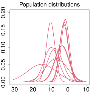
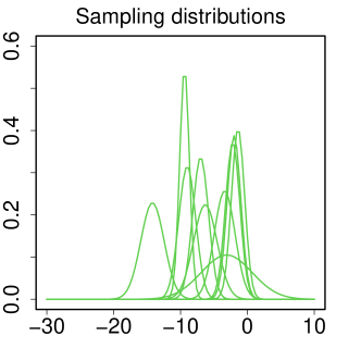
Figure 2: Population distributions of the ten studies and the sampling distributions of the observed effect sizes. For each study, the population distribution is assumed to be normal with mean $y_{i}$ and variance $n_{i}\hat{\sigma}_{y_{i}}^{2}$. The sampling distribution of the effect size is assumed to be normal with mean $y_{i}$ and variance $\hat{\sigma}_{y_{i}}^{2}$.

To further compare the $I^{2}_{\rm A}$ statistic and the $I^{2}$ statistic, as a common practice we assume that the 10 studies are all normally distributed. Then by the reported means and variances, we plot their respective population distributions and the sampling distributions of the observed effect sizes in Figure 2 for visualization. From the figure, it is evident that the 10 studies are not very heterogeneous since most of the study populations are largely overlapped in the range roughly from -15 to 5, corresponding to a measure of 0.41 for the $I^{2}_{\rm A}$ statistic. By contrast, the sampling distributions of the observed effect sizes are less overlapped with each other, indicating a much higher heterogeneity at 0.92 by the $I^{2}$ statistic.

4.2 Numerical results

To conduct simulations that compare the performance of the $I^{2}_{\rm A}$ statistic to the $I^{2}$ statistic, we consider the random-effects model (5) with $\mu=0$ and $\sigma^{2}=100$. For the between-study variance, we consider $\tau^{2}=9$ or 90 that corresponds to ${\rm ICC}_{\rm MA}$ as $9/(9+100)=0.083$ or $90/(90+100)=0.474$, respectively. We also let $k=3$ or 10 to represent the small or large number of studies included in the meta-analysis. For the sample size of each study, we consider the unbalanced design with the sample size of the $i$th study being $i*n$, where $i=1,\dots,k$ and the common $n$ ranges from 10 to 100. With each of the above settings, we then generate the raw data from model (5) and report the summary data $y_{i}$ and $\hat{\sigma}_{y_{i}}^{2}$ for the $k$ studies. Finally with $M=10,000$ repetitions, we compute the mean values of the $I^{2}_{\rm A}$ and $I^{2}$ statistics and plot them in Figure 3.

From Figure 3, it is evident that the $I^{2}$ statistic is always monotonically increasing with the sample size $n$. This is consistent with what was observed in Rücker et al., (2008) that the $I^{2}$ statistic always increases rapidly to 1 when the sample sizes are large. By contrast, with each dashed line representing the heterogeneity ${\rm ICC}_{\rm MA}$ between the study populations, we note that the performance of the $I^{2}_{\rm A}$ statistic is not impacted by the sample size. And more interesting, it can perform even better when the number of studies $k$ is large, which coincides with the asymptotic results on the consistent estimates of the unknown quantities.

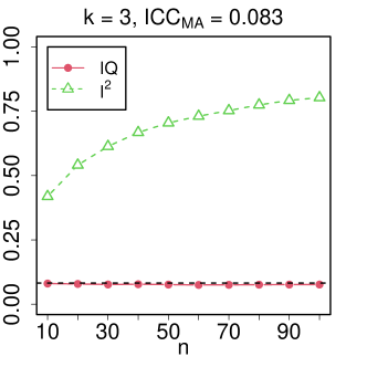
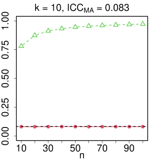
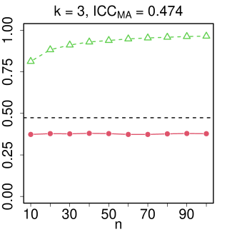
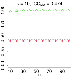
Figure 3: Simulated mean values of the two statistics for the raw mean with 10,000 repetitions. The red lines with circles represent the $I^{2}_{\rm A}$ statistic, the green lines with triangles represent the $I^{2}$ statistic, and the dashed lines stand for the absolute heterogeneity ${\rm ICC}_{\rm MA}$.

5 The $I^{2}_{\rm A}$ statistic for the mean difference

In this section, we apply the mean difference between the two treatment arms as the effect size, which is also referred to as the raw mean difference. For a meta-analysis of the mean difference, the summary statistics for each study often include the observed mean differences between treatment and control groups $y_{i}$, the sample sizes $n_{i}^{T}$ and $n_{i}^{C}$, and the standard errors $\hat{\sigma}_{y_{i}^{T}}$ and $\hat{\sigma}_{y_{i}^{C}}$. By defining the adjusted sample size as $n_{i}=1/(1/n_{i}^{T}+1/n_{i}^{C})$ for each study, ${\rm MSB}_{\rm MA}$ and $\bar{n}$ can be computed by formulas (8) and (10), respectively. Moreover, ${\rm MSW}_{\rm MA}$ can be computed by

$${\rm MSW}_{\rm MA} = \frac{\sum_{i=1}^{k}\left\{n_{i}^{T}\left(n_{i}^{T}-1\right)\hat{\sigma}^{2}_{y^{T}_{i}}+n_{i}^{C}\left(n_{i}^{C}-1\right)\hat{\sigma}^{2}_{y^{C}_{i}}\right\}}{\sum_{i=1}^{k}\left(n_{i}^{T}+n_{i}^{C}\right)-2k}.$$

Finally, the $I^{2}_{\rm A}$ statistic can be computed directly by formula (11). For a comprehensive understanding of the model specification and the whole procedure for estimating the $I^{2}_{\rm A}$ statistic, one may refer to Appendix C.

5.1 Real data analysis

To exemplify the utilization of the $I^{2}_{\rm A}$ statistic for the mean differences, we revisit a meta-analysis conducted in a study by Avery et al., (2022). This study explores the effect of interventions to taper long term opioid treatment for chronic non-cancer pain. Among the several interventions, we consider the effect of acupuncture. For each study, the observed effect size is the mean difference of reduced opioid dose. For easy reference, we provide the summary data for the three studies in Table 3.

Table 3: Summary data of the 3 studies for the meta-analysis from Avery et al. (2022).

Study	$y_{i}^{T}$	$n_{i}^{T}$	$\hat{\sigma}_{y_{i}^{T}}$	$y_{i}^{C}$	$n_{i}^{C}$	$\hat{\sigma}_{y_{i}^{C}}$
Jackson (2021)	-34	9	10.43	-66	6	12.78
Zheng (2019)	-13.6	48	3.23	-8.8	60	3.14
Zheng (2008)	-25.7	17	7.59	-10.9	18	2.80

By Table 3, the estimated effect sizes $y_{i}$ for the three studies are computed as 32.0, -4.8 and -14.8, and the adjusted sample sizes $n_{i}$ for the three studies are 3.60, 26.67 and 8.74, respectively. From these values, we can further obtain $\bar{y}=-3.65$, ${\rm MSB}_{\rm MA}=2848.76$, ${\rm MSW}_{\rm MA}=586.93$, and the adjusted mean sample size $\bar{n}=9.24$. Finally, by formula (11), it yields that

$$I^{2}_{\rm A}=\max\left\{\frac{2848.76-586.93}{2848.76+(9.24-1)\times 586.93},0\right\}=0.29.$$

To compute the $I^{2}$ statistic, we first derive the within-study variances of $y_{i}$ as 272.14, 20.29 and 65.48, respectively. Then we have $\sum_{i=1}^{3}w_{i}=0.07$ and $\sum_{i=1}^{3}w_{i}y_{i}=0.35$. This leads to Cochran’s $Q$ statistic as $Q=6.50$. Moreover, by formula (3), we have

$$I^{2}=\max\left\{\frac{6.50-(3-1)}{6.50},0\right\}=0.69.$$

To further compare the $I^{2}_{\rm A}$ and $I^{2}$ statistics, we also plot the population distributions for the three studies and the sampling distributions of the observed effect sizes in Figure 4 for visualization. We note that two of the populations are largely overlapped with little heterogeneity, whereas the third population is moderately deviated. Given this, we conclude that the heterogeneity among the three studies may not be substantial overall, if measured by the $I^{2}_{\rm A}$ statistic. By contrast, the $I^{2}$ statistic concludes a very substantial heterogeneity between the sampling distributions of the observed effect sizes.

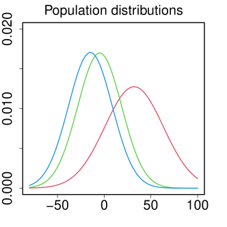
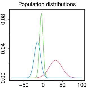
Figure 4: Population distributions of the three studies and the sampling distributions of the observed effect sizes with blue for Zheng (2008), green for Zheng (2019), and red for Jackson (2021). For each study, the population distribution is assumed to be normal with mean $y_{i}^{T}-y_{i}^{C}$ and variance $\{n_{i}^{T}(n_{i}^{T}-1)\hat{\sigma}_{y_{i}^{T}}^{2}+n_{i}^{C}(n_{i}^{C}-1)\hat{\sigma}_{y_{i}^{C}}^{2}\}/(n_{i}^{T}+n_{i}^{C}-2)$. The sampling distribution of the effect size is assumed to be normal with mean $y_{i}^{T}-y_{i}^{C}$ and variance $\hat{\sigma}_{y_{i}^{T}}^{2}+\hat{\sigma}_{y_{i}^{C}}^{2}$.

5.2 Numerical results

To numerically compare the $I^{2}_{\rm A}$ and $I^{2}$ statistics, we generate the data from two-arm studies as follows:

$$\begin{aligned} y_{ij}^{T}&=\mu^{T}+\delta_{i}^{T}+\xi_{ij}^{T},\quad j=1,\ldots,n_{i}^{T},\\ y_{ij^{\prime}}^{C}&=\mu^{C}+\delta_{i}^{C}+\xi_{ij^{\prime}}^{C},\quad j^{\prime}=1,\ldots,n_{i}^{C},\end{aligned}$$ (14)

where $\xi_{ij}^{T}$ and $\xi_{ij^{\prime}}^{C}$ are i.i.d. normal random errors with mean 0 and common variance $\sigma^{2}$. For a more detailed description of model (14), one may refer to Appendix Appendix D.

Without loss of generality, we set $\mu^{T}=\mu^{C}=0$ and $\sigma^{2}=1$. We also generate $\delta_{i}^{T}$ and $\delta_{i}^{C}$ independently from $N(0,0.045)$ or $N(0,0.45)$. With the observed effect sizes being $\sum_{j=1}^{n^{T}}y_{ij}^{T}/n_{i}^{T}-\sum_{j^{\prime}=1}^{n^{C}}y_{ij^{\prime}}^{C}/n_{i}^{C}$, the between-study variance is $\tau^{2}=0.09$ or $0.9$, yielding an ${\rm ICC}_{\rm MA}$ value of $0.083$ or $0.474$, respectively. For other settings, we consider $k=3$ or 10 to represent a small or large number of studies within the meta-analysis, and the sample sizes of both treatment arms, $n_{i}^{T}$ and $n_{i}^{C}$, to be identical. We further let the sample sizes for both arms of the $i$th study be $i*n$, where $i$ ranges from 1 to $k$, and $n$ varies from 10 to 100. Then for each simulation setting, we proceed to generate the raw data and compute the summary statistics, including $y_{i}^{T}$, $y_{i}^{C}$, $\hat{\sigma}_{y_{i}^{T}}^{2}$ and $\hat{\sigma}_{y_{i}^{C}}^{2}$, for each of the $k$ studies. Finally with $M=10,000$ repetitions, we calculate and visualize the mean values of the $I^{2}_{\rm A}$ and $I^{2}$ statistics in Figure 5.

From Figure 5, we once again observe that the $I^{2}$ statistic monotonically increases with the sample size $n$. On the other hand, the performance of the $I^{2}_{\rm A}$ statistic is not impacted by the sample size, and meanwhile it performs even better when the number of studies $k$ is large.

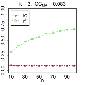
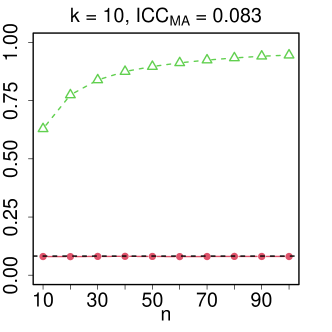
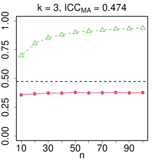
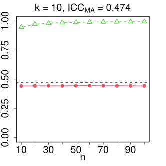
Figure 5: Simulated mean values of the two statistics for the mean difference with 10,000 repetitions. The red lines with circles represent the $I^{2}_{\rm A}$ statistic, the green lines with triangles represent the $I^{2}$ statistic, and the dashed lines stand for the absolute heterogeneity ${\rm ICC}_{\rm MA}$.

6 The $I^{2}_{\rm A}$ statistic for the standardized mean difference

In addition to the mean difference (MD), another commonly used effect size for continuous outcomes in two-arm studies is the standardized mean difference (SMD). The SMD is particularly useful when the assumption of equal population variances across different studies cannot be made. In such cases, the mean difference in each study is standardized to a uniform scale, ensuring comparability for the subsequent meta-analysis. Consequently, the estimated standardized mean difference $y_{i}$ can be viewed as the observed mean difference of two population arms, both with a variance of 1, indicating $\sigma_{\rm pop}^{2}=1$.

To compute the $I^{2}_{\rm A}$ statistic for SMD, we employ the same procedures as those used for MD to determine ${\rm MSB}_{\rm MA}$ and $\bar{n}$. More specifically, considering the summary statistics including the observed SMD $y_{i}$, the sample sizes $n_{i}^{C}$ for the control groups, and the sample sizes $n_{i}^{T}$ for the treatment groups, in conjunction with the adjusted sample sizes $n_{i}=1/(1/n_{i}^{C}+1/n_{i}^{T})$ for each study, we compute ${\rm MSB}_{\rm MA}$ and $\bar{n}$ by formulas (8) and (10), respectively. Further by $\sigma_{\rm pop}^{2}=1$, we also set ${\rm MSW}_{\rm MA}$ directly to 1. Ultimately, the heterogeneity among the studies can be quantified by the $I^{2}_{\rm A}$ statistic as described in (11). For a comprehensive understanding of the model specifications as well as the methodology for estimating the $I^{2}_{\rm A}$ statistic, one may refer to Appendix Appendix E.

6.1 Real data analysis

To assess the utility of the $I^{2}_{\rm A}$ statistic in quantifying the heterogeneity for SMD, we revisit the real data example presented in Section 5.1. With the summary data provided in Table 3, we first compute the estimated SMD and its corresponding variance for each study. Two commonly used statistics for estimating SMD are Cohen’s $d$ (Cohen,, 2013) and Hedges’ $g$ (Hedges,, 1981). For a detailed guide on computing Cohen’s $d$ and Hedges’ $g$, one may refer to Lin and Aloe, (2021). In this section, we employ Hedges’ $g$ that derives an unbiased estimate for SMD.

By the formulas provided in Lin and Aloe, (2021), we can derive the estimated SMDs for the three studies as 0.96, -0.20 and -0.62, and the adjusted sample sizes $n_{i}$ as 3.60, 26.67 and 8.74, respectively, Moreover, we have $\bar{y}=-0.19$, ${\rm MSB}_{\rm MA}=3.19$, ${\rm MSW}_{\rm MA}=1$, and the adjusted mean sample size $\bar{n}=9.24$. Finally, by formula (11), the $I^{2}_{\rm A}$ statistic is given as

$$I^{2}_{\rm A}=\max\left\{\frac{3.19-1}{3.19+(9.24-1)\times 1},0\right\}=0.19.$$

To compute the $I^{2}$ statistic, we first derive the within-study variances of $y_{i}$ as 0.31, 0.04 and 0.12, respectively. Further with $\sum_{i=1}^{3}w_{i}=38.12$ and $\sum_{i=1}^{3}w_{i}y_{i}=-7.43$, Cochran’s $Q$ statistic can be computed as $Q=5.83$. Finally, by formula (3), we have

$$I^{2}=\max\left\{\frac{5.83-(3-1)}{5.83},0\right\}=0.66.$$

To further compare the two statistics, we plot the scaled population distributions for the three studies and the sampling distributions of the observed effect sizes in Figure 6. Specifically, with SMDs as the effect sizes, all the scaled populations have a common variance of 1. Moreover, we apply the estimated SMDs as the population means. Compared to Figure 4, the three scaled populations in Figure 6 get more close to each other, resulting in a even smaller value for the $I^{2}_{\rm A}$ statistic. On the other hand, a measure of 0.66 for the $I^{2}$ statistic indicates a large heterogeneity between the observed effect sizes.

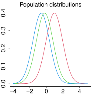
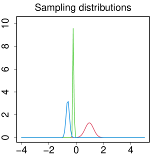
Figure 6: Population distributions of the three scaled studies and the sampling distributions of the observed effect sizes with blue for Zheng (2008), green for Zheng (2019), and red for Jackson (2021). For each study, the population distribution is assumed to be normal with mean SMD and variance 1. The sampling distribution of the effect size is assumed to be normal with mean SMD and the variance is assumed to be the within-study variance.

6.2 Numerical results

To compare the $I^{2}_{\rm A}$ and $I^{2}$ statistics for SMD, we generate the data from the following two-arm studies:

$$\begin{aligned} y_{ij}^{T}&=\sigma_{i}(\mu^{T}+\delta_{i}^{T}+\xi_{ij}^{T}),\quad j=1,\ldots,n_{i}^{T},\\ y_{ij^{\prime}}^{C}&=\sigma_{i}(\mu^{C}+\delta_{i}^{C}+\xi_{ij^{\prime}}^{C}),\quad j^{\prime}=1,\ldots,n_{i}^{C},\end{aligned}$$ (15)

where $\xi_{ij}^{T}$ and $\xi_{ij^{\prime}}^{C}$ are i.i.d. normal random errors with mean 0 and variance 1. Compared with model (14), this new model contains an additional parameter $\sigma_{i}$, which is used to rescale each study. For a more detailed description of model (15), one may refer to Appendix Appendix E.

In this simulation, we let $\sigma_{i}$ follow a uniform distribution $U(0.5,1.5)$, which yields unequal population variances for the $k$ studies and thus SMD ought to be applied rather than MD. The other settings are kept the same as those in Section 6.2. Then for each simulation setting, we proceed to generate the raw data and compute the summary statistics, including $y_{i}^{T}$, $y_{i}^{C}$, $\hat{\sigma}_{y_{i}^{T}}^{2}$ and $\hat{\sigma}_{y_{i}^{C}}^{2}$, for each of the $k$ studies. Finally with $M=10,000$ repetitions, we compute and plot the mean values of the $I^{2}_{\rm A}$ and $I^{2}$ statistics in Figure 7.

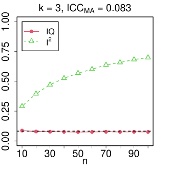
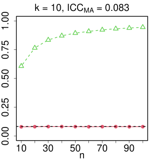
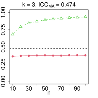
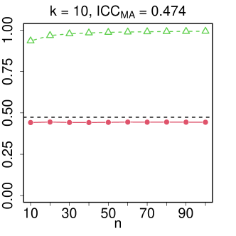
Figure 7: Simulated mean values of the two statistics for the mean difference with 10,000 repetitions. The red lines with circles represent the $I^{2}_{\rm A}$ statistic, the green lines with triangles represent the $I^{2}$ statistic, and the dashed lines stand for the absolute heterogeneity ${\rm ICC}_{\rm MA}$.

From Figure 7, it is evident that the $I^{2}$ statistic is always monotonically increasing with the sample size $n$, which is consistent with the simulation results in Sections 4.2 and 5.2. By contrast, the $I^{2}_{\rm A}$ statistic can always provide a good measure for the quantify of heterogeneity between the study populations, no matter whether the study sample sizes are large or not.

7 Conclusion and discussion

Quantifying the heterogeneity is an important issue in meta-analysis for decision making. The presence of heterogeneity affects the extent to which generalizable conclusions can be formed and determines whether the random-effects model or the fixed-effect model should be employed. The $Q$ statistic is commonly used to test for the existence of the heterogeneity. However, as mentioned in the Cochrane Handbook for Systematic Reviews of Interventions (Higgins et al.,, 2019), this test may have lowe power when the number of studies is small. Some also argue that the heterogeneity always exists, whether detectable by statistical tests or not. Thus, as a way to remedy, the $I^{2}$ statistic was further introduced to measure the extent of heterogeneity. Nowadays, both the $Q$ statistic and the $I^{2}$ statistic are routinely reported in the forest plot in meta-analysis, and the choice between the random-effects model and the fixed-effect model often relies on these two statistics. More specifically, if the $p$-value of the $Q$ statistic is less than 0.1 and the $I^{2}$ statistic exceeds 0.5, the random-effects model is preferred for meta-analysis; otherwise, the fixed-effect model will be chosen (Jiang and Huang,, 2021; Chinnaratha et al.,, 2016; Yang et al.,, 2012). It is noted, however, that these two statistics are highly correlated since the $I^{2}$ statistic is a monotonically increasing function of the $Q$ statistic. Additionally, the $p$-value based on the $Q$ statistic only indicates whether there is a statistical significance (Gelman and Stern,, 2006), but not reflect regarding the biological difference between the studies.

In this paper, we have introduced a new measure, denoted as ${\rm ICC}_{\rm MA}$, to quantify the between-study heterogeneity for meta-analysis. To explore the distinction between ${\rm ICC}_{\rm HT}$ and ${\rm ICC}_{\rm MA}$, we have also drawn an interesting connection between ANOVA and meta-analysis, and learned that the essence of ${\rm ICC}_{\rm HT}$ is to quantify the heterogeneity between the observed effect sizes. As demonstrated by the motivating example in Section 2, the sampling distributions of the observed effect sizes may exhibit a significant dependency on the sample sizes, and they will asymptotically converge to their true effect sizes. Accordingly, with large sample sizes, the observed effect sizes will also yield an increased ${\rm ICC}_{\rm HT}$ close to one, no matter whether the underlying heterogeneity between the study populations is truly large or not.

As an important alternative, our newly defined ${\rm ICC}_{\rm MA}$ is proposed to directly quantify the heterogeneity between the study populations. More specifically, we have systematically studied the statistical properties of ${\rm ICC}_{\rm MA}$, including the monotonicity, the location and scale invariance, the study size invariance, and the sample size invariance. It is the sample size invariance that distinguishes our new absolute measure of heterogeneity from ${\rm ICC}_{\rm HT}$. Moreover, we have also proposed the $I^{2}_{\rm A}$ statistic to serve as the estimator of ${\rm ICC}_{\rm MA}$. The footnote “A” represents that that we are to estimate the absolute measure of heterogeneity in meta-analysis. For practical use, the exact formulas for the $I^{2}_{\rm A}$ statistic are also derived under two common scenarios with the mean difference or the standardized mean difference as the effect size. Simulations and real data analysis demonstrate that the $I^{2}_{\rm A}$ statistic provides an asymptotically unbiased estimator of the absolute heterogeneity between the study populations, and as expected, it also does not depend on the study sample sizes. To conclude, the $I^{2}_{\rm A}$ statistic can serve as a supplemental measure to monitor the situations where the study effect sizes are indeed similar with little biological difference. In such scenario, the fixed-effect model can be appropriate. Whereas if the sample sizes are very large, we note that the $I^{2}$ statistic may still rapidly increase to 1 showing a large heterogeneity and subsequently a random-effects model will continue to be adopted. In view of this, we are thus confident that the $I^{2}_{\rm A}$ statistic can add new value to meta-analysis, for example, being included in the forest plot as a supplement to the $I^{2}$ statistic.

Lastly, it is worth noting that there are also several interesting directions for future research. First, the current work has presented its primary focus on meta-analysis with continuous outcomes. As a parallel work, it can be equally important for the $I^{2}_{\rm A}$ statistic to be further extended to meta-analysis with binary outcomes, which are also commonly encountered in clinical studies. Second, it is of interest to study whether the $I^{2}_{\rm A}$ statistic can be further improved, and in particular, by Figures 3, 5 and 7, we note that the $I^{2}_{\rm A}$ statistic tends to slightly underestimate ${\rm ICC}_{\rm MA}$ when $k$ is small and ${\rm ICC}_{\rm MA}$ is large. In addition, future research may also be warranted to, more deeply, explore the practical performance of the $I^{2}_{\rm A}$ statistic in evidence-based practice.

Appendix Appendix A Proof of the properties of ICC_MA

Proof of “Monotonicity”.

By the definition in (7), we can rewrite ICC_MA as

$${\rm ICC}_{\rm MA}=\frac{1}{1+\sigma_{\rm pop}^{2}/\tau^{2}}.$$

This shows that ICC_MA is a monotonically increasing function of $\tau^{2}/\sigma_{\rm pop}^{2}$ and so property (i^′) holds. ∎

Proof of “Location and scale invariance”.

To prove the location and scale invariance, for any constants $a$ and $b>0$, we assume that the newly observed effect sizes are $y^{\prime}_{ij}=a+by_{ij}$ for $i=1,\ldots,k$ and $j=1,\ldots,n_{i}$. Let also $\mu^{\prime}_{i}=a+b\mu_{i}$ be the true effect sizes of the new study populations. Then consequently, the between-study variance and the common population variance are given as

$$(\tau^{2})^{\prime} = {\rm var}(\mu^{\prime}_{i})={\rm var}(a+b\mu_{i})=b^{2}\tau^{2},$$

$$(\sigma_{\rm pop}^{2})^{\prime} = {\rm var}(a+by_{ij}|a+b\mu_{i})=b^{2}\sigma_{\rm pop}^{2}.$$

Further by (7), the measure of heterogeneity between the new studies is

$${\rm ICC}^{\prime}_{\rm MA}=\frac{(\tau^{2})^{\prime}}{(\tau^{2})^{\prime}+(\sigma_{\rm pop}^{2})^{\prime}}=\frac{b^{2}\tau^{2}}{b^{2}\tau^{2}+b^{2}\sigma_{\rm pop}^{2}}=\frac{\tau^{2}}{\tau^{2}+\sigma_{\rm pop}^{2}}={\rm ICC}_{\rm MA}.$$

This verifies the property of location and scale invariance. ∎

Proof of “Study size invariance”.

To prove the study size invariance, we assume there are a total of $k^{\prime}$ studies. Then by the random-effects model in (1), since the individual means $\mu_{i}$ are i.i.d. from $N(\mu,\tau^{2})$, the between-study variance will remain unchanged as $\tau^{2}$ regardless of the number of studies. Further by the common population variance assumption, we have ${\rm var}(y_{ij}|\mu_{i})=\sigma_{\rm pop}^{2}$ for all $i=1,\dots,k^{\prime}$ and $j=1,\dots,n_{i}$. This proves the property of study size invariance. ∎

Proof of “Sample size invariance”.

To prove the sample size invariance, we assume that the new sample sizes are $n_{i}^{\prime}$ for each study, and consequently $y_{i}^{\prime}=\sum_{j=1}^{n_{i}^{\prime}}y_{ij}/n_{i}^{\prime}$ are the new effect sizes. Then under the common population variance assumption that ${\rm var}(y_{ij}|\mu_{i})=\sigma_{\rm pop}^{2}$ for all $i$ and $j$, we have $\sigma_{y_{i}^{\prime}}^{2}={\rm var}(y_{i}^{\prime}|\mu_{i})=\sigma_{\rm pop}^{2}/n_{i}^{\prime}$, or equivalently, $n_{i}^{\prime}\sigma_{y_{i}^{\prime}}^{2}=\sigma_{\rm pop}^{2}$. That is, no matter how the sample sizes vary, the common population variance will always remain unchanged. Finally, noting that $\tau^{2}$ also remains since the study populations are unaltered, we thus have the property of sample size invariance. ∎

Appendix Appendix B Methods for estimating ICC

To estimate ICC from the random-effects ANOVA in (4), we first partition the total variation of the observations into two components as

$$\sum_{i=1}^{k}\sum_{j=1}^{n_{i}}(y_{ij}-\bar{y})^{2}=\sum_{i=1}^{k}n_{i}(y_{i}-\bar{y})^{2}+\sum_{i=1}^{k}\sum_{j=1}^{n_{i}}(y_{ij}-y_{i})^{2},$$ (16)

where $y_{i}=\sum_{j=1}^{n_{i}}y_{ij}/n_{i}$ are the individual sample means, and $\bar{y}=\sum_{i=1}^{k}\sum_{j=1}^{n_{i}}y_{ij}/\sum_{i=1}^{k}n_{i}$ is the grand sample mean. More specifically, the term on the left-hand side of (16) is the total sum of squares (SST), and the two terms on the right-hand side are the sum of squares between the populations (SSB) and the error sum of squares within the populations (SSW), respectively.

By equating SSB and SSW to their respective expected values, Cochran, (1939) derived the method of moments estimators of $\tau^{2}$ and $\sigma^{2}$. Further by plugging these two estimators in formula (6), it yields the ANOVA estimator for the unknown ICC. By Smith, (1957), the ANOVA estimator is a biased but consistent estimator. Moreover, as the method of moments estimators may take a negative value when ${\rm SSB}/k<{\rm SSW}/(\sum_{i=1}^{k}(n_{i}-1)$, one often truncates the negative value to 0 when it occurs. For the balanced case when the sample sizes are all equal, Searle, (1971) derived an exact confidence interval for ICC based on the ANOVA table. For the unbalanced case, however, the exact confidence interval from the ANOVA table is not available. As a remedy, Thomas and Hultquist, (1978) and Donner, (1979) suggested an adjusted confidence interval in which the common sample size in the balanced case is replaced by the average sample size. They further showed by simulation studies that the adjusted confidence interval performs very well in terms of the coverage probability.

Besides the well-known ANOVA estimator, it is noteworthy that there are also other estimators for ICC in the literature. To name a few, Thomas and Hultquist, (1978) constructed a confidence interval for ICC based on the unweighted average of the individual sample means $\tilde{y}=\sum_{i=1}^{k}y_{i}/k$. Observing that ${\rm ICC}=(\tau^{2}/\sigma^{2})/(\tau^{2}/\sigma^{2}+1)$, Wald, (1940) proposed another estimator for ICC by first estimating $\tau^{2}/\sigma^{2}$, yet as a limitation, there does not exist a closed form for either the point estimator or its confidence interval. As another alternative, by the facts that ${\rm cov}(y_{ij},y_{il})=\tau^{2}$ for $j\neq l$ and ${\rm var}(y_{ij})=\tau^{2}+\sigma^{2}$, Karlin et al., (1981) proposed to estimate ICC by the Pearson product-moment correlation computed over all the possible pairs of $(y_{ij},y_{il})$ for $j\neq l$ with some weighting schemes. In addition, Donner and Koval, 1980a ; Donner and Koval, 1980b proposed an iterative algorithm to compute the maximum likelihood estimator (MLE) for ICC directly, and presented its performance by simulations when the number of studies is large. For more estimators of ICC, one may also refer to Donner, (1986), Sahai and Ojeda, (2004), and the references therein.

Despite the rich literature on the estimation of ICC, none of the existing estimators is known to be uniformly better than the others in the unbalanced case (Sahai and Ojeda,, 2004). In practice, thanks to its simple and elegant form, the ANOVA estimator is frequently treated as the optimal estimator and so is most commonly used for estimating ICC. Lastly, we also note that the ANOVA estimator and the confidence interval suggested by Thomas and Hultquist, (1978) and Donner, (1979) can be readily implemented by the function ICCest in the R package ‘ICC’.

Appendix Appendix C The derivation of the point estimate (10) and the confidence interval (11) for ${\rm ICC}_{\rm MA}$

To prove the properties of the point estimator and the confidence interval for ${\rm ICC}_{\rm MA}$ in (11) and (12), we first give the proofs of the two lemmas.

Proof of Lemma 1.

Denote by $\sigma_{y_{i}}^{2}=\sigma^{2}/n_{i}$. With the summary data, $y_{i}$ are independent normal random variables with mean $\mu$ and variances $\tau^{2}+\sigma_{y_{i}}^{2}$. Then the variance of $\sum_{i=1}^{k}n_{i}y_{i}$ is

$${\rm Var}\left(\sum_{i=1}^{k}n_{i}y_{i}\right)=\sum_{i=1}^{k}{\rm Var}\left(n_{i}y_{i}\right)=\tau^{2}\sum_{i=1}^{k}n_{i}^{2}+\sum_{i=1}^{k}n_{i}^{2}\sigma_{y_{i}}^{2}.$$

Thus,

$$E\left(\sum_{i=1}^{k}n_{i}y_{i}\right)^{2} = {\rm Var}\left(\sum_{i=1}^{k}n_{i}y_{i}\right)+\left\{E\left(\sum_{i=1}^{k}n_{i}y_{i}\right)\right\}^{2}$$

$$= \tau^{2}\sum_{i=1}^{k}n_{i}^{2}+\sum_{i=1}^{k}n_{i}^{2}\sigma_{y_{i}}^{2}+\mu^{2}\left(\sum_{i=1}^{k}n_{i}\right)^{2}.$$

Further, it can be derived that

$$E\left\{\sum_{i=1}^{k}n_{i}\left(y_{i}-\bar{y}\right)^{2}\right\}$$

$$= \sum_{i=1}^{k}n_{i}E\left(y_{i}^{2}\right)-\frac{1}{\sum_{i=1}^{k}n_{i}}E\left(\sum_{i=1}^{k}n_{i}y_{i}\right)^{2}$$

$$= \sum_{i=1}^{k}n_{i}\left[{\rm Var}\left(y_{i}\right)+\left\{E\left(y_{i}\right)\right\}^{2}\right]-\frac{1}{\sum_{i=1}^{k}n_{i}}E\left(\sum_{i=1}^{k}n_{i}y_{i}\right)^{2}$$

$$= \sum_{i=1}^{k}n_{i}\left(\tau^{2}+\sigma_{y_{i}}^{2}+\mu^{2}\right)-\frac{1}{\sum_{i=1}^{k}n_{i}}\left\{\tau^{2}\sum_{i=1}^{k}n_{i}^{2}+\sum_{i=1}^{k}n_{i}^{2}\sigma_{y_{i}}^{2}+\mu^{2}(\sum_{i=1}^{k}n_{i})^{2}\right\}$$

$$= \tau^{2}(\sum_{i=1}^{k}n_{i}-\frac{\sum_{i=1}^{k}n^{2}_{i}}{\sum_{i=1}^{k}n_{i}})+\sum_{i=1}^{k}n_{i}\sigma^{2}_{y_{i}}-\frac{\sum_{i=1}^{k}n^{2}_{i}\sigma^{2}_{y_{i}}}{\sum_{i=1}^{k}n_{i}}.$$

Since $\sigma_{y_{i}}^{2}=\sigma_{\rm pop}^{2}/n_{i}$, and $\bar{n}=(\sum_{i=1}^{k}n_{i}-\sum_{i=1}^{k}n^{2}_{i}/\sum_{i=1}^{k}n_{i})/(k-1)$,

$$E\left\{\sum_{i=1}^{k}n_{i}\left(y_{i}-\bar{y}\right)^{2}\right\} = (k-1)\bar{n}\tau^{2}+(k-1)\sigma_{\rm pop}^{2}.$$

Thus, $E({\rm MSB}_{\rm MA})=\bar{n}\tau^{2}+\sigma_{\rm pop}^{2}$.

As for $E({\rm MSW}_{\rm MA})=\sigma_{\rm pop}^{2}$, it is derived directly by the fact that $E(n_{i}\hat{\sigma}^{2}_{y_{i}})=\sigma_{\rm pop}^{2}$. ∎

Proof of Lemma 2.

With model (4) and the notations in Lemma 1, $y_{i}$ is independent of $n\hat{\sigma}^{2}_{y_{i}}$ for $i=1,\dots,k$. Given that ${\rm MSB}_{\rm MA}$ is a function of $y_{i}$, and ${\rm MSW}_{\rm MA}$ is a function of $n\hat{\sigma}^{2}_{y_{i}}$, they are independent of each other. Besides, let $n$ be the common sample size, the adjusted mean sample size $\bar{n}$ reduces to $n$ for the balanced case.

Let $\mathbf{Y}=(y_{1},\dots,y_{k})^{\mbox{\tiny{T}}}$, $\Sigma={\rm Var}(\mathbf{Y})=(\tau^{2}+\sigma_{y}^{2})\mathbf{I}_{k}$ with $\mathbf{I}_{k}$ being the $k\times k$ identity matrix, and ${\bf 1}_{k}$ be the column vector of length $k$ with all the elements being 1. Let $\mathbf{Z}\sim N(0,\mathbf{I}_{k})$. Then $\mathbf{Y}$ can be expressed as $\mathbf{Y}=\Sigma^{1/2}\mathbf{Z}+\mu{\bf 1}_{k}=(\tau^{2}+\sigma_{y}^{2})^{1/2}\mathbf{Z}+\mu{\bf 1}_{k}$. By the above notations, $\sum_{i=1}^{k}n\left(y_{i}-\bar{y}\right)^{2}$ can be written as

$$\sum_{i=1}^{k}n\left(y_{i}-\bar{y}\right)^{2} = n\mathbf{Y}^{\mbox{\tiny{T}}}\left(\mathbf{I}_{k}-\frac{1}{k}{\bf 1}_{k}{\bf 1}_{k}^{\mbox{\tiny{T}}}\right)\mathbf{Y}$$

$$= n\left(\Sigma^{1/2}\mathbf{Z}+\mu{\bf 1}_{k}\right)^{\mbox{\tiny{T}}}\left(\mathbf{I}_{k}-\frac{1}{k}{\bf 1}_{k}{\bf 1}_{k}^{\mbox{\tiny{T}}}\right)\left(\Sigma^{1/2}\mathbf{Z}+\mu{\bf 1}_{k}\right)$$

$$= (n\tau^{2}+n\sigma_{y}^{2}){\mathbf{Z}}^{\mbox{\tiny{T}}}\left(\mathbf{I}_{k}-\frac{1}{k}{\bf 1}_{k}{\bf 1}_{k}^{\mbox{\tiny{T}}}\right){\mathbf{Z}}.$$

Note that $(\mathbf{I}_{k}-\frac{1}{k}{\bf 1}_{k}{\bf 1}_{k}^{\mbox{\tiny{T}}})$ is an idempotent matrix with rank $k-1$. So it can be decomposed as $(\mathbf{I}_{k}-\frac{1}{k}{\bf 1}_{k}{\bf 1}_{k}^{\mbox{\tiny{T}}})=\mathbf{V}\Lambda\mathbf{V}^{\mbox{\tiny{T}}}$, where $\Lambda={\rm diag}(1,\dots,1,0)$ and $\mathbf{V}=({\bf v}_{1},\dots,{\bf v}_{k})$ is an orthogonal matrix. With ${\bf v}_{i}^{\mbox{\tiny{T}}}\mathbf{Z}\stackrel{{\scriptstyle\text{i.i.d.}}}{{\sim}}N(0,1)$, the distribution of $\sum_{i=1}^{k}\left(y_{i}-\bar{y}\right)^{2}$ can be derived as

$$\sum_{i=1}^{k}n\left(y_{i}-\bar{y}\right)^{2} = \left(n\tau^{2}+n\sigma_{y}^{2}\right)\left(\mathbf{V}^{\mbox{\tiny{T}}}{\mathbf{Z}}\right)^{\mbox{\tiny{T}}}\Lambda\left(\mathbf{V}^{\mbox{\tiny{T}}}{\mathbf{Z}}\right)$$

$$= \left(n\tau^{2}+n\sigma_{y}^{2}\right)\sum_{i=1}^{k-1}\left({\bf v}_{i}^{\mbox{\tiny{T}}}\mathbf{Z}\right)^{2}$$

$$= \left(n\tau^{2}+n\sigma_{y}^{2}\right)\chi^{2}_{k-1}$$

$$= \{n\tau^{2}+\sigma_{\rm pop}^{2}\}\chi^{2}_{k-1}.$$

Thus, ${\rm MSB}_{\rm MA}=\sum_{i=1}^{k}\{n(y_{i}-\bar{y})^{2}\}/(k-1)$ is distributed with $\{n\tau^{2}+\sigma_{\rm pop}^{2}\}\chi^{2}_{k-1}/(k-1)$.

Since $(n-1)n\hat{\sigma}_{y_{i}}^{2}$ follow distributions $\sigma_{\rm pop}^{2}\chi^{2}_{n-1}$ and are independent of each other for $i=1,\dots,k$, ${\rm MSW}_{\rm MA}\sim\sigma_{\rm pop}^{2}\chi^{2}_{k(n-1)}/\{k(n-1)\}$. ∎

Derivation of (11) and (12)..

With Lemma 1, $E({\rm MSB}_{\rm MA}-{\rm MSW}_{\rm MA})=\bar{n}\tau^{2}$, and $E\{{\rm MSB}_{\rm MA}+(\bar{n}-1){\rm MSW}_{\rm MA}\}=\bar{n}(\tau^{2}+\sigma_{\rm pop}^{2})$. Thus, ${\rm ICC}_{\rm MA}=\tau^{2}/(\tau^{2}+\sigma_{\rm pop}^{2})$ can be estimated by $({\rm MSB}_{\rm MA}-{\rm MSW}_{\rm MA})/\{{\rm MSB}_{\rm MA}+(\bar{n}-1){\rm MSW}_{\rm MA}\}$. Truncating the negative value to zero, the $I^{2}_{\rm A}$ statistic in (11) can be derived.

Denote $F_{k-1,k(\bar{n}-1)}$ by the $F$ distribution with $k-1$ and $k(\bar{n}-1)$ degrees of freedom. Let $F_{\alpha}$ be the $(100\alpha)$th percentile of $F_{k-1,k(\bar{n}-1)}$ and $\bar{F}_{\rm MA}={\rm MSB}_{\rm MA}/{\rm MSW}_{\rm MA}$. Then with Lemma 2, under the balanced case, $\sigma_{\rm pop}^{2}/(\bar{n}\tau^{2}+\sigma_{\rm pop}^{2})\cdot\bar{F}_{\rm MA}$ is distributed with $F_{k-1,k(\bar{n}-1)}$. We have

$$1-\alpha = \Pr\left(F_{\alpha/2}\leq\frac{\sigma_{\rm pop}^{2}}{\bar{n}\tau^{2}+\sigma_{\rm pop}^{2}}\bar{F}_{\rm MA}\leq F_{1-\alpha/2}\right)$$

$$= \Pr\left(\bar{F}_{\rm MA}/F_{1-\alpha/2}\leq\frac{\bar{n}\tau^{2}+\sigma_{\rm pop}^{2}}{\sigma_{\rm pop}^{2}}\leq\bar{F}_{\rm MA}/F_{\alpha/2}\right)$$

$$= \Pr\left\{\frac{1}{\bar{n}}\left(\bar{F}_{\rm MA}/F_{1-\alpha/2}-1\right)\leq\frac{\tau^{2}}{\sigma_{\rm pop}^{2}}\leq\frac{1}{\bar{n}}\left(\bar{F}_{\rm MA}/F_{\alpha/2}-1\right)\right\}.$$

For the left inequality,

$$\Pr\left\{\frac{1}{\bar{n}}\left(\bar{F}_{\rm MA}/F_{1-\alpha/2}-1\right)\leq\frac{\tau^{2}}{\sigma_{\rm pop}^{2}}\right\}$$

$$= \Pr\left\{\frac{1}{\bar{n}}\left(\bar{F}_{\rm MA}/F_{1-\alpha/2}-1\right)\leq 0\right\}+\Pr\left(\frac{\tau^{2}+\sigma_{\rm pop}^{2}}{\tau^{2}}\leq\frac{\bar{n}+\bar{F}_{\rm MA}/F_{1-\alpha/2}-1}{\bar{F}_{\rm MA}/F_{1-\alpha/2}-1}\right)$$

$$= \Pr\left(\frac{\bar{F}_{\rm MA}/F_{1-\alpha/2}-1}{\bar{n}+\bar{F}_{\rm MA}/F_{1-\alpha/2}-1}\leq\frac{\tau^{2}}{\tau^{2}+\sigma_{\rm pop}^{2}}\right).$$

For the right inequality,

$$\Pr\left\{\frac{\tau^{2}}{\sigma_{\rm pop}^{2}}\leq\frac{1}{\bar{n}}\left(\bar{F}_{\rm MA}/F_{\alpha/2}-1\right)\right\}$$

$$= \Pr\left\{\frac{1}{\bar{n}}\left(\bar{F}_{\rm MA}/F_{\alpha/2}-1\right)>0,\frac{\bar{n}+\bar{F}_{\rm MA}/F_{\alpha/2}-1}{\bar{F}_{\rm MA}/F_{\alpha/2}-1}\leq\frac{\tau^{2}+\sigma_{\rm pop}^{2}}{\tau^{2}}\right\}$$

$$= \Pr\left(\frac{\tau^{2}}{\tau^{2}+\sigma_{\rm pop}^{2}}\leq\frac{\bar{F}_{\rm MA}/F_{\alpha/2}-1}{\bar{n}+\bar{F}_{\rm MA}/F_{\alpha/2}-1}\right).$$

Thus, the $100(1-\alpha)\%$ confidence interval for ${\rm ICC}_{\rm MA}$ is

$$\left[\frac{\bar{F}_{\rm MA}/F_{1-\alpha/2}-1}{\bar{n}+\bar{F}_{\rm MA}/F_{1-\alpha/2}-1},~{}\frac{\bar{F}_{\rm MA}/F_{\alpha/2}-1}{\bar{n}+\bar{F}_{\rm MA}/F_{\alpha/2}-1}\right].$$

The confidence interval in (12) is derived by truncating the negative values of the above limits to zero. ∎

Appendix Appendix D The derivation of the $I^{2}_{\rm A}$ statistic for the mean difference

To generalize the $I^{2}_{\rm A}$ statistic to mean difference, we also start with modeling the individual patient data in a single study. In analogy with model (4), we model the individual observations $y_{ij}^{T}$ and $y_{ij^{\prime}}^{C}$ of the treatment group and the control group for the $i$th study as

$$\begin{aligned} y_{ij}^{T}&=\mu^{T}+\delta_{i}^{T}+\xi_{ij}^{T},\quad j=1,\ldots,n_{i}^{T},\\ y_{ij^{\prime}}^{C}&=\mu^{C}+\delta_{i}^{C}+\xi_{ij^{\prime}}^{C},\quad j^{\prime}=1,\ldots,n_{i}^{C},\end{aligned}$$

where the superscript “T” represents the treatment group, and the superscript “C” represents the control group. Similar to the assumptions in model (4), we assume that $\delta_{i}^{T}$, $\xi_{ij^{\prime}}^{T}$, $\delta_{i}^{C}$ and $\xi_{ij^{\prime}}^{C}$ are independent of each other. For the random errors of different observations in the same study, it is natural to assume they are i.i.d. normal random errors with mean 0 and share a common variance $\sigma^{2}$. Then the true effect size for each study is routinely presented by the mean difference

$${\rm MD}_{i}=(\mu^{T}+\delta_{i}^{T})-(\mu^{C}+\delta_{i}^{C}).$$

For each study, the observed mean difference is

$$y_{i}^{T}-y_{i}^{C}=(\mu^{T}-\mu^{C})+(\delta_{i}^{T}-\delta_{i}^{C})+(\frac{\sum_{j=1}^{n_{i}^{T}}\xi_{ij}}{n_{i}^{T}}-\frac{\sum_{j^{\prime}=1}^{n_{i}^{C}}\xi_{ij}}{n_{i}^{C}}),$$ (17)

where $y_{i}^{T}=\sum_{j=1}^{n^{T}}\xi_{ij}/n_{i}^{T}$, and $y_{i}^{C}=\sum_{j=1}^{n^{C}}\xi_{ij}/n_{i}^{C}$. Further, let $y_{i}=y_{i}^{T}-y_{i}^{C}$, $\mu=\mu^{T}-\mu^{C}$, $\delta_{i}=\delta_{i}^{T}-\delta_{i}^{C}$, and $\epsilon_{i}=\sum_{j=1}^{n_{i}^{T}}\xi_{ij}/n_{i}^{T}-\sum_{j^{\prime}=1}^{n_{i}^{C}}\xi_{ij}/n_{i}^{C}$. Regardless of the dependence between $\delta_{i}^{T}$ and $\delta_{i}^{C}$, we simply assume that $\delta_{i}$ are i.i.d. normal random variables with mean 0 and variance $\tau^{2}\geq 0$, where $\tau^{2}$ measures the magnitude of the heterogeneity between studies. Then model (17) reduces to

$$y_{i}=\mu+\delta_{i}+\epsilon_{i},$$ (18)

where $\delta_{i}\stackrel{{\scriptstyle\text{i.i.d.}}}{{\sim}}N(0,\tau^{2})$ and $\epsilon_{i}\stackrel{{\scriptstyle\text{ind}}}{{\sim}}N(0,(1/n_{i}^{T}+1/n_{i}^{C})\sigma^{2})$. We note that model (18) has the same form as in (5), except for the variance of $\epsilon_{i}$. To estimate ${\rm ICC}_{\rm MA}$ for the mean difference, we apply the results for the single-arm studies directly. Letting $n_{i}=1/(1/n_{i}^{T}+1/n_{i}^{C})$, Lemma 1 in Appendix Appendix B also holds that

$$E({\rm MSB}_{\rm MA}) = \bar{n}\tau^{2}+\sigma^{2},$$

$$E({\rm MSW}_{\rm MA}) = \sigma^{2}.$$

Together with the notation of $\bar{n}$, the $I^{2}_{\rm A}$ statistic in (11) can be derived.

Appendix Appendix E The derivation of the $I^{2}_{\rm A}$ statistic for the standardized mean difference

For the standardized mean difference, we model the individual observations $y_{ij}^{T}$ and $y_{ij^{\prime}}^{C}$ of the treatment group and the control group for the $i$th study as

$$\begin{aligned} y_{ij}^{T}&=\sigma_{i}(\mu^{T}+\delta_{i}^{T}+\xi_{ij}^{T}),\quad j=1,\ldots,n_{i}^{T},\\ y_{ij^{\prime}}^{C}&=\sigma_{i}(\mu^{C}+\delta_{i}^{C}+\xi_{ij^{\prime}}^{C}),\quad j^{\prime}=1,\ldots,n_{i}^{C},\end{aligned}$$

where the superscript “T” represents the treatment group, and the superscript “C” represents the control group. Similar to the assumptions in model (4), we assume that $\delta_{i}^{T}$, $\xi_{ij^{\prime}}^{T}$, $\delta_{i}^{C}$ and $\xi_{ij^{\prime}}^{C}$ are independent of each other. In (ipdsmd), $\xi_{ij^{\prime}}^{T}$ and $\xi_{ij^{\prime}}^{C}$ are assumed to be i.i.d. normal random errors with mean 0 and variance 1. Then with different values of $\sigma_{i}$, the population variances for different studies are $\sigma_{i}^{2}$, respectively. To eliminate the influence of the scale, SMDs are considered to represent the effect sizes, which is defined by

$${\rm SMD}_{i} = \{(\sigma_{i}\mu^{T}+\sigma_{i}\delta_{i}^{T})-(\sigma_{i}\mu^{C}+\sigma_{i}\delta_{i}^{C})\}/\sigma_{i}=(\mu^{T}+\delta_{i}^{T})-(\mu^{C}+\delta_{i}^{C}).$$

For each study, SMD_i is estimated by

$$\frac{y_{i}^{T}-y_{i}^{C}}{\hat{\sigma}_{i}}=\frac{\sigma_{i}}{\hat{\sigma}_{i}}\{(\mu^{T}-\mu^{C})+(\delta_{i}^{T}-\delta_{i}^{C})+(\frac{\sum_{j=1}^{n_{i}^{T}}\xi_{ij}}{n_{i}^{T}}-\frac{\sum_{j^{\prime}=1}^{n_{i}^{C}}\xi_{ij}}{n_{i}^{C}})\},$$ (19)

where $\hat{\sigma}_{i}$ is an estimate for $\sigma_{i}$, $y_{i}^{T}=\sum_{j=1}^{n^{T}}\xi_{ij}/n_{i}^{T}$, and $y_{i}^{C}=\sum_{j=1}^{n^{C}}\xi_{ij}/n_{i}^{C}$. For simplicity, we assume that $\sigma_{i}$ can be accurately estimated and thus $\sigma_{i}/\hat{\sigma}_{i}=1$. Further, let $y_{i}=y_{i}^{T}-y_{i}^{C}$, $\mu=\mu^{T}-\mu^{C}$, $\delta_{i}=\delta_{i}^{T}-\delta_{i}^{C}$, and $\epsilon_{i}=\sum_{j=1}^{n_{i}^{T}}\xi_{ij}/n_{i}^{T}-\sum_{j^{\prime}=1}^{n_{i}^{C}}\xi_{ij}/n_{i}^{C}$. Regardless of the dependence between $\delta_{i}^{T}$ and $\delta_{i}^{C}$, we simply assume that $\delta_{i}$ are i.i.d. normal random variables with mean 0 and variance $\tau^{2}\geq 0$, where $\tau^{2}$ measures the magnitude of the heterogeneity between studies. Then model (19) reduces to

$$y_{i}=\mu+\delta_{i}+\epsilon_{i},$$ (20)

where $\delta_{i}\stackrel{{\scriptstyle\text{i.i.d.}}}{{\sim}}N(0,\tau^{2})$ and $\epsilon_{i}\stackrel{{\scriptstyle\text{ind}}}{{\sim}}N(0,1/n_{i}^{T}+1/n_{i}^{C})$. We note that model (20) has the same form as in (5), except for the variance of $\epsilon_{i}$. To estimate ${\rm ICC}_{\rm MA}$ for the mean difference, we also apply the results for the single-arm studies directly. Letting $n_{i}=1/(1/n_{i}^{T}+1/n_{i}^{C})$, Lemma 1 in Appendix Appendix B also holds that

$$E({\rm MSB}_{\rm MA}) = \bar{n}\tau^{2}+1.$$

Together with the notation of $\bar{n}$ and ${\rm MSB}_{\rm MA}=1$, the $I^{2}_{\rm A}$ statistic in (11) can be derived.

References

- Avery et al., (2022) Avery, N., McNeilage, A. G., Stanaway, F., Ashton-James, C. E., Blyth, F. M., Martin, R., Gholamrezaei, A., and Glare, P. (2022). Efficacy of interventions to reduce long term opioid treatment for chronic non-cancer pain: systematic review and meta-analysis. British Medical Journal, 377:e066375.
- Böhning et al., (2017) Böhning, D., Lerdsuwansri, R., and Holling, H. (2017). Some general points on the -measure of heterogeneity in meta-analysis. Metrika, 80(6):685–695.
- Borenstein et al., (2017) Borenstein, M., Higgins, J. P., Hedges, L. V., and Rothstein, H. R. (2017). Basics of meta-analysis: is not an absolute measure of heterogeneity. Research Synthesis Methods, 8(1):5–18.
- Chinnaratha et al., (2016) Chinnaratha, M. A., Chuang, M.-y. A., Fraser, R. J., Woodman, R. J., and Wigg, A. J. (2016). Percutaneous thermal ablation for primary hepatocellular carcinoma: a systematic review and meta-analysis. Journal of Gastroenterology and Hepatology, 31(2):294–301.
- Cochran, (1939) Cochran, W. G. (1939). The use of the analysis of variance in enumeration by sampling. Journal of the American Statistical Association, 34(207):492–510.
- Cochran, (1954) Cochran, W. G. (1954). The combination of estimates from different experiments. Biometrics, 10(1):101–129.
- Cohen, (2013) Cohen, J. (2013). Statistical Power Analysis for the Behavioral Sciences, 2nd Edition. New York: Routledge.
- DerSimonian and Laird, (1986) DerSimonian, R. and Laird, N. (1986). Meta-analysis in clinical trials. Controlled Clinical Trials, 7(3):177–188.
- Donner, (1979) Donner, A. (1979). The use of correlation and regression in the analysis of family resemblance. American Journal of Epidemiology, 110(3):335–342.
- Donner, (1986) Donner, A. (1986). A review of inference procedures for the intraclass correlation coefficient in the one-way random effects model. International Statistical Review, 54(1):67–82.
- (11) Donner, A. and Koval, J. J. (1980a). The estimation of intraclass correlation in the analysis of family data. Biometrics, 36(1):19–25.
- (12) Donner, A. and Koval, J. J. (1980b). The large sample variance of an intraclass correlation. Biometrika, 67(3):719–722.
- EFSA Scientific Committee, (2011) EFSA Scientific Committee (2011). Statistical significance and biological relevance. EFSA Journal, 9(9):2372.
- Egger and Smith, (1997) Egger, M. and Smith, G. D. (1997). Meta-analysis: potentials and promise. British Medical Journal, 315(7119):1371–1374.
- Fisher, (1925) Fisher, R. A. (1925). Statistical Methods for Research Workers. Edinburgh: Oliver & Boyd.
- Gelman and Stern, (2006) Gelman, A. and Stern, H. (2006). The difference between “significant” and “not significant” is not itself statistically significant. The American Statistician, 60(4):328–331.
- Hedges, (1981) Hedges, L. V. (1981). Distribution theory for glass’s estimator of effect size and related estimators. Journal of Educational Statistics, 6(2):107–128.
- Higgins et al., (2019) Higgins, J. P., Thomas, J., Chandler, J., Cumpston, M., Li, T., Page, M. J., and Welch, V. A. (2019). Cochrane Handbook for Systematic Reviews of Interventions, 2nd Edition. Chichester: John Wiley & Sons.
- Higgins and Thompson, (2002) Higgins, J. P. and Thompson, S. G. (2002). Quantifying heterogeneity in a meta-analysis. Statistics in Medicine, 21(11):1539–1558.
- Higgins et al., (2003) Higgins, J. P., Thompson, S. G., Deeks, J. J., and Altman, D. G. (2003). Measuring inconsistency in meta-analyses. British Medical Journal, 327(7414):557–560.
- Holling et al., (2020) Holling, H., Böhning, W., Masoudi, E., Böhning, D., and Sangnawakij, P. (2020). Evaluation of a new version of with emphasis on diagnostic problems. Communications in Statistics-Simulation and Computation, 49(4):942–972.
- IntHout et al., (2016) IntHout, J., Ioannidis, J. P., Rovers, M. M., and Goeman, J. J. (2016). Plea for routinely presenting prediction intervals in meta-analysis. BMJ Open, 6(7):e010247.
- Jeong et al., (2014) Jeong, H., Yim, H. W., Cho, Y. S., Kim, Y. I., Jeong, S. N., Kim, H. B., and Oh, I. H. (2014). Efficacy and safety of stem cell therapies for patients with stroke: a systematic review and single arm meta-analysis. International Journal of Stem Cells, 7(2):63–69.
- Jiang and Huang, (2021) Jiang, S.-J. and Huang, C.-H. (2021). The clinical efficacy of n-acetylcysteine in the treatment of st segment elevation myocardial infarction a meta-analysis and systematic review. International Heart Journal, 62(1):142–147.
- Karlin et al., (1981) Karlin, S., Cameron, E. C., and Williams, P. T. (1981). Sibling and parent–offspring correlation estimation with variable family size. Proceedings of the National Academy of Sciences of the United States of America, 78(5):2664–2668.
- Lin and Aloe, (2021) Lin, L. and Aloe, A. M. (2021). Evaluation of various estimators for standardized mean difference in meta-analysis. Statistics in Medicine, 40(2):403–426.
- McGraw and Wong, (1996) McGraw, K. O. and Wong, S. P. (1996). Forming inferences about some intraclass correlation coefficients. Psychological Methods, 1(1):30–46.
- Riley et al., (2016) Riley, R. D., Ensor, J., Snell, K. I., Debray, T. P., Altman, D. G., Moons, K. G., and Collins, G. S. (2016). External validation of clinical prediction models using big datasets from e-health records or IPD meta-analysis: opportunities and challenges. British Medical Journal, 353(8063):i3140.
- Rücker et al., (2008) Rücker, G., Schwarzer, G., Carpenter, J. R., and Schumacher, M. (2008). Undue reliance on in assessing heterogeneity may mislead. BMC Medical Research Methodology, 8(1):79.
- Sahai and Ojeda, (2004) Sahai, H. and Ojeda, M. M. (2004). Analysis of Variance for Random Models: Theory, Methods, Applications, and Data Analysis. Volume 2: Unbalanced Data. Boston: Birkhäuser.
- Sangnawakij et al., (2019) Sangnawakij, P., Böhning, D., Niwitpong, S. A., Adams, S., Stanton, M., and Holling, H. (2019). Meta-analysis without study-specific variance information: heterogeneity case. Statistical Methods in Medical Research, 28(1):196–210.
- Searle, (1971) Searle, S. R. (1971). Linear Models. New York: Wiley.
- Smith, (1957) Smith, C. A. B. (1957). On the estimation of intraclass correlation. Annals of Human Genetics, 21(4):363–373.
- Thomas and Hultquist, (1978) Thomas, J. D. and Hultquist, R. A. (1978). Interval estimation for the unbalanced case of the one-way random effects model. The Annals of Statistics, 6(3):582–587.
- Wald, (1940) Wald, A. (1940). A note on the analysis of variance with unequal class frequencies. The Annals of Mathematical Statistics, 11(1):96–100.
- Yang et al., (2012) Yang, J., Wang, H.-P., Zhou, L., and Xu, C.-F. (2012). Effect of dietary fiber on constipation: a meta analysis. World Journal of Gastroenterology, 18(48):7378.