Consistency of pion form factor and unpolarized transverse momentum dependent parton distributions beyond leading twist in the light-front quark model

Abstract

We investigate the interplay among the pion’s form factor, transverse momentum dependent distributions (TMDs), and parton distribution functions (PDFs) extending our light-front quark model (LFQM) computation based on the Bakamjian-Thomas construction for the two-point function Jafar1 ; Jafar2 to the three-point and four-point functions. Ensuring the four-momentum conservation at the meson-quark vertex from the Bakamjian-Thomas construction, the meson mass is taken consistently as the corresponding invariant meson mass both in the matrix element and the Lorentz factor in our LFQM computation. We achieve the current-component independence in the physical observables such as the pion form factor and delve into the derivation of unpolarized TMDs and PDFs associated with the forward matrix element. We address the challenges posed by twist-4 TMDs and exhibit the fulfillment of the sum rule. Effectively, our LFQM successfully handles the light-front zero modes and offers insights for broader three-point and four-point functions and related observables.

I Introduction

Comprehending the internal structure of the pion is a paramount objective in modern nuclear and particle physics. Being the lightest meson comprised of quark and antiquark recognized as a pseudo-Goldstone boson of Quantum Chromodynamics (QCD), the pion provides an unparalleled opportunity to delve into the intricacies of strong interactions. In particular, several different aspects of pion structure such as its decay constant, distribution amplitudes (DAs), form factors, parton distribution functions (PDFs), generalized parton distributions (GPDs), and transverse momentum dependent distributions (TMDs) offer complementary insights into how quarks and gluons are distributed in terms of their charge, momentum, and spatial positions BL80 ; PW99 ; DS1 ; Lorce ; LPS16 ; TB18 ; Barry18 .

Alongside the experimental measurement Amen84 ; Dally82 ; Amen86 ; Volmer ; Tade ; Horn of the pion’s decay constant and elastic form factor, one can also investigate the partonic structure of the pion by directing pion beams at nuclear targets using the Drell-Yan process (DY) DY70 . In fact, the DY process not only grants access to the pion’s twist-2 PDF Owen ; Gluck ; SMRS ; Gluck99 ; WRH but also furnishes information about TMDs, encompassing both leading and subleading twists AMS09 . In particular, as elucidated in Lorce ; LPS16 , the exploration of higher-twist TMDs and PDFs not only offers insights into quark-gluon dynamics but also serves as a means to assess the internal consistency of phenomenological models.

The light-front quark model (LFQM) SLF2 ; SLF3 ; CCH96 ; CP05 ; CJ97 ; CJ99a ; CJ07 ; Choi07 ; CJLR15 ; ACJO22 based on the light-front dynamics (LFD) BPP stands as a powerful theoretical framework for unraveling the intricate details of aforementioned aspects of hadron structure and related phenomena. In the LFQM, the pion form factor $F_{\pi}(Q^{2})$, derived from the components of the vector currents $J^{\mu}$ with $\mu=(+,\perp,-)$, is linked Lorce ; LPS16 to the twist-2, 3, and 4 TMDs in the forward matrix elements of $J^{\mu}$ respectively. While the form factor and TMDs obtained from $J^{+}(=J^{0}+J^{3})$ and ${\bf J}_{\perp}=(J_{x},J_{y})$ remain unaffected by the LF zero modes, it is well-known that both $F_{\pi}(Q^{2})$ and the twist-4 TMD obtained from the $J^{-}(=J^{0}-J^{3})$ current is prone to receive contributions from the zero modes. The presence of zero-mode contributions from the $J^{-}$ current poses challenges to the internal consistency of the LFQM in the computation of the twist-4 pion TMD, as discussed in Lorce ; LPS16 . While the presence of LF zero mode resulting from the $J^{-}$ current appears to be a universal feature to be investigated in LFD, its specific quantitative contribution relies on the choice of model wave functions characterizing the bound state of hadrons Jaus99 ; Melo12 ; Melo02 ; CJ98 ; BCJ01 ; BCJ02 . Therefore, it is of paramount importance to correctly extract and incorporate the zero modes specific to a given LFQM examining its self-consistency.

Over the past several years, we have developed our self-consistent LFQM that allows us to obtain the physical observables in a manner independent of the current components. We noticed that the self-consistency of LFQM adheres to the Bakamjian-Thomas (BT) construction principle BT53 ; KP91 . The interaction $V_{q{\bar{q}}}$ between quark and antiquark is incorporated into the mass operator via $M:=M_{0}+V_{q{\bar{q}}}$ in line with the BT construction as we have shown in our LFQM analysis of mass spectra for the ground and radially excited states of pseudoscalar and vector mesons can be found in  CJ97 ; CJ99a ; CJLR15 ; ACJO22 . In this framework, the meson state is constructed from non-interacting, on-mass shell quark and antiquark representations, with a strict adherence to the four momentum conservation $P=p_{q}+p_{{\bar{q}}}$ at the meson-quark vertex, where $P$ and $p_{q({\bar{q}})}$ represent the momenta of the meson and quark (antiquark), respectively. In particular, the conservation of LF energy ($P^{-}=p^{-}_{q}+p^{-}_{\bar{q}}$) at the meson-quark vertex signifies the importance of taking the meson mass as the invariant mass $M_{0}$ in terms of the quark and antiquark momenta to satisfy $\frac{{M^{2}_{0}}+{{\bf P}^{2}_{\perp}}}{P^{+}}=\left(\frac{{p^{+2}_{q}}+{{\bf p}^{2}_{q\perp}}}{p^{+}_{q}}+\frac{{p^{+2}_{\bar{q}}}+{{\bf p}^{2}_{{\bar{q}}\perp}}}{p^{+}_{\bar{q}}}\right)$ in the computation of the meson-quark vertex.

In contrast to traditional LFQM approaches SLF2 ; SLF3 ; CCH96 , the distinguished feature of our self-consistent LFQM lies in the computation of hadronic matrix elements. For instance, consider the transition matrix element $\langle P^{\prime}|{\bar{q}}\Gamma^{\mu}q|P\rangle={\cal P}^{\mu}{\cal F}$, where ${\cal F}$ represents various physical observables like decay constants and form factors. ${\cal P}^{\mu}$ corresponds to the associated Lorentz factors. In traditional LFQM SLF2 ; SLF3 ; CCH96 , when calculating ${\cal F}$, the BT construction (i.e., setting $M\to M_{0}$) is only applied to the matrix element $\langle P^{\prime}|{\bar{q}}\Gamma^{\mu}q|P\rangle$ and not to the Lorentz factor ${\cal P}^{\mu}$. This selective application of $M\to M_{0}$ solely to the matrix element results in the LF zero mode affecting the observable ${\cal F}$, particularly when using the “bad” component of the current, such as the minus current. We have found CJ14 ; CJ15 ; CJ17 ; Jafar1 ; Jafar2 ; Choi21 ; ChoiAdv , however, that it is necessary to apply the consistent BT construction or replacement ($M\to M_{0}$) equally to both the matrix element and the Lorentz factor in order to obtain ${\cal F}$ as independent of the current components as we have shown CJ14 ; CJ15 ; CJ17 ; Jafar1 ; Jafar2 ; Choi21 ; ChoiAdv in the computation of the decay constants of pseudoscalar and vector mesons together with the leading-and higher-twist DAs CJ14 ; CJ15 ; CJ17 ; Jafar1 ; Jafar2 and weak transition form factors Choi21 ; ChoiAdv between two pseudoscalar mesons. This can be achieved by computing ${\cal F}=\bra{P^{\prime}}\frac{\Gamma^{\mu}}{{\cal P}^{\mu}}\ket{P}$, meaning that the Lorentz factor should be computed within the integral of internal momenta. To signify this unique and novel prescription consistent with the BT construction in the computation of physical observables, we may coin our LFQM as “self-consistent” LFQM.

In Refs. CJ14 ; CJ15 ; CJ17 ; Jafar1 ; Jafar2 ; Choi21 ; ChoiAdv , we have also developed our self-consistent LFQM by starting from the manifestly covariant Bethe-Salpeter (BS) model. Within this derivation, we identified a distinct matching condition, denoted as the “type II” link (e.g., see Eq. (49) in CJ14 ). This type II link plays a pivotal role in connecting the covariant BS model to our LFQM, ensuring its adherence to the principles of the BT construction. Notably, a crucial component of the type II link involves substituting the physical meson mass $M$ that originally appeared in the integrand for the matrix element calculation with the invariant mass $M_{0}$. This replacement aligns with the principles of the BT construction within our LFQM framework.

The primary aim of the present work is to utilize the self-consistency of the LFQM in deriving the correlated pion’s form factor, TMDs, and PDFs. Our focus is on recognizing the intricate relationships between these quantities while addressing the twist structure present in TMDs and PDFs, categorized by the components of the current $J^{\mu}$. Of particular note is our unique theoretical approach, which leverages the BT construction to compute the form factor, twist-4 TMDs, and PDFs derived from the minus component of the currents. We think that this approach represents a novel and original contribution within the framework of the LFQM.

The paper is organized as follows: In Sec. II, we illustrate the essential aspect of the LFQM consistent with the BT construction in the two-point function computation of the decay constant and distribution amplitude. The current component independence of the decay constant is exemplified in this section along with the computation of the leading-twist DA both at the initial scale $\mu^{2}_{0}=1$ GeV² and at the scale $\mu^{2}=10$ GeV² through QCD evolution. In Sec. III, we extend the computation to the three-point function describing the general structure of the pseudoscalar meson form factor and obtain the current component independent pion form factor. In Sec. IV, we further extend our computation to the four-point function and obtain the three unpolarized TMDs related with the forward matrix element $\langle P|{\bar{q}}\gamma^{\mu}q|P\rangle$, where the twist-2, 3, and 4 TMDs are obtained from $\mu=+,\perp$, and $-$, respectively. The twist-2, 3, 4 PDFs obtained from the corresponding TMDs are also presented in this section. Especially, we resolve the LF zero mode issue of the twist-4 TMD and PDF in our LFQM. We also discuss the QCD evolution of a pion PDFs and present the Mellin moments of the three PDFs compared with other theoretical predictions. Finally, we summarize our findings in Sec. V. In the Appendix A, we display the results for the helicity contributions to the pion form factor. In the Appendix B, the type II link between the manifestly covariant BS model and the self-consistent LFQM is demonstrated for completeness. The influence of the quark running mass on the pion form factor by treating mass evolution solely as a function of the momentum transfer $Q^{2}$ is also examined in Appendix C.

II Light-Front Quark Model Application to Pion Decay constant and distribution amplitude

The essential aspect of the LFQM SLF2 ; SLF3 ; CCH96 ; CP05 ; CJ97 ; CJ99a ; CJ07 for the $q{\bar{q}}$ bound state meson with the total momentum $P=(P^{+},P^{-},{\bf P}_{\perp})$ is to saturate the Fock state expansion by the constituent $q$ and ${\bar{q}}$ and treat the Fock state in a noninteracting $q{\bar{q}}$ representation while the interaction is added to the mass operator via $M:=M_{0}+V_{q\bar{q}}$, to satisfy the Poincaré group structure, i.e. the commutation relations for the system of two-particle bound state. The interactions are then encoded in the LF wave function $\Psi_{\lambda_{q}\lambda_{\bar{q}}}^{JJ_{z}}({\bf p}_{q},{\bf p}_{\bar{q}})$, which is the eigenfunction of the mass operator. The meson state $\ket{M(P,J,J_{z})}\equiv\ket{\cal M}$ of momentum $P$ and spin $(J,J_{z})$ can be constructed as

$$\ket{\mathcal{M}} = \int\left[{\rm d}^{3}{\bf p}_{q}\right]\left[{\rm d}^{3}{\bf p}_{\bar{q}}\right]2(2\pi)^{3}\delta^{3}\left({\bf P}-{\bf p}_{q}-{\bf p}_{\bar{q}}\right)$$ (1)

$$\times\mbox{}\sum_{\lambda_{q},\lambda_{\bar{q}}}\Psi_{\lambda_{q}\lambda_{\bar{q}}}^{JJ_{z}}({\bf p}_{q},{\bf p}_{\bar{q}})\ket{q(p_{q},\lambda_{q})\bar{q}(p_{\bar{q}},\lambda_{\bar{q}})},\quad$$

where $p^{\mu}_{q(\bar{q})}$ and $\lambda_{q(\bar{q})}$ are the momenta and the helicities of the on-mass shell $(p_{q(\bar{q})}^{2}=m^{2}_{q(\bar{q})})$ constituent quark (antiquark), respectively. Here, $\left[{\rm d}^{3}{\bf p}\right]\equiv{\rm d}p^{+}{\rm d}^{2}\mathbf{p}_{\perp}/(16\pi^{3})$. The LF on-shell momenta $p_{q(\bar{q})}$ of $q({\bar{q}})$ are defined in terms of the LF relative momentum variables $(x,{\bf k}_{\perp})$ as

$$p^{+}_{q}=xP^{+},\;\;p^{+}_{\bar{q}}=(1-x)P^{+},$$

$${\bf p}_{q\perp}=x{\bf P}_{\perp}-{\bf k}_{\perp},\;\;{\bf p}_{{\bar{q}}\perp}=(1-x){\bf P}_{\perp}+{\bf k}_{\perp},$$ (2)

which satisfies $(p_{q}+p_{\bar{q}})^{2}=M^{2}_{0}$. If one defines the longitudinal momentum fraction $x$ in terms of the momentum variable $k_{z}$ as SLF2 ; SLF3

$$x=\frac{E_{1}+k_{z}}{E_{1}+E_{2}},\;\;1-x=\frac{E_{2}-k_{z}}{E_{1}+E_{2}},$$ (3)

where $E_{i}=\sqrt{m^{2}_{i}+{\vec{k}}^{2}}$ is the kinetic energy of $i$th-constituent and ${\vec{k}}=({\bf k}_{\perp},k_{z})$ so that $M_{0}=E_{1}+E_{2}$. For the equal quark and antiquark mass case ($E_{1}=E_{2}=E$), $M^{2}_{0}=4E^{2}$ and $k_{z}=(x-\frac{1}{2})M_{0}$.

In terms of the LF relative momentum variable $(x,{\bf k}_{\perp})$, the boost-invariant meson mass squared is given by

$$M^{2}_{0}=\frac{{\bf k}^{2}_{\perp}+m^{2}}{x}+\frac{{\bf k}^{2}_{\perp}+m^{2}}{1-x},$$ (4)

where $m=m_{q}=m_{\bar{q}}$ for the pion case. The LF wave function of the pion is generically given by

$$\Psi_{\lambda_{q}{\lambda_{\bar{q}}}}(x,{\bf k}_{\perp})=\phi(x,{\bf k}_{\perp}){\cal R}_{\lambda_{q}{\lambda_{\bar{q}}}}(x,{\bf k}_{\perp}),$$ (5)

where $\phi(x,{\bf k}_{\perp})$ is the radial wave function and ${\cal R}_{\lambda_{q}{\lambda_{\bar{q}}}}(x,{\bf k}_{\perp})$ is the spin-orbit wave function that is obtained by the interaction independent Melosh transformation Melosh from the ordinary spin-orbit wave function assigned by the quantum number $J^{PC}$. The covariant form of ${\cal R}_{\lambda_{q}{\lambda_{\bar{q}}}}$ for the pion is given by SLF2 ; SLF3

$${\cal R}_{\lambda_{q}{\lambda_{\bar{q}}}}=\frac{\bar{u}_{\lambda_{q}}(p_{q})\gamma_{5}v_{\lambda_{\bar{q}}}(p_{\bar{q}})}{\sqrt{2}M_{0}},$$ (6)

and it satisfies $\sum_{\lambda^{\prime}s}{\cal R}^{\dagger}{\cal R}=1$. The explicit matrix form of ${\cal R}_{\lambda_{q}{\lambda_{\bar{q}}}}$ for the pion is given by

$${\cal R}_{\lambda_{q}{\lambda_{\bar{q}}}}=\frac{1}{\sqrt{2p^{+}_{q}p^{+}_{\bar{q}}}M_{0}}\left(\begin{array}[]{cc}p^{+}_{q}p^{L}_{\bar{q}}-p^{L}_{q}p^{+}_{\bar{q}}&m(p^{+}_{q}+p^{+}_{\bar{q}})\\ -m(p^{+}_{q}+p^{+}_{\bar{q}})&p^{+}_{q}p^{R}_{\bar{q}}-p^{R}_{q}p^{+}_{\bar{q}}\end{array}\right),\;$$ (7)

where $p^{R(L)}=p_{x}\pm ip_{y}$. Eq. (7) can be expressed in terms of $(x,{\bf k}_{\perp})$ variables defined in Eq. (II).

The interactions between $q$ and ${\bar{q}}$ are included in the mass operator BT53 ; KP91 to compute the mass eigenvalue of the meson state. In our LFQM, we treat the radial wave function $\phi(x,{\bf k}_{\perp})$ as a trial function for the variational principle to the QCD-motivated effective Hamiltonian saturating the Fock state expansion by the constituent $q$ and ${\bar{q}}$. The QCD-motivated Hamiltonian for a description of the ground and radially excited meson mass spectra is then given by $H_{q\bar{q}}\ket{\Psi}=(M_{0}+V_{q\bar{q}})\ket{\Psi}=M_{q{\bar{q}}}\ket{\Psi}$, where $M_{q{\bar{q}}}$ and $\Psi=\Psi_{\lambda_{q}\lambda{\bar{q}}}$ are the mass eigenvalue and eigenfunction of the $q{\bar{q}}$ meson, respectively. The detailed mass spectroscopic analysis for the ground and radially excited mesons can be found in Refs. CJ97 ; CJ99a ; CJ09 ; CJLR15 ; ACJO22 .

For the $1S$ state radial wave function $\phi(x,{\bf k}_{\perp})$, we use the Gaussian wave function

$$\phi(x,{\bf k}_{\perp})=\frac{4\pi^{3/4}}{\beta^{3/2}}\sqrt{\frac{\partial k_{z}}{\partial x}}{\rm exp}(-{\vec{k}}^{2}/2\beta^{2}),$$ (8)

where $\beta$ is the variational parameter fixed by the analysis of meson mass spectra CJ97 ; CJ99a ; CJ09 . For $m_{q}=m_{\bar{q}}=m$ case, the Jacobian of the variable transformation $\{x,{\bf k}_{\perp}\}\to{\vec{k}}=({\bf k}_{\perp},k_{z})$ is given by $\frac{\partial k_{z}}{\partial x}=\frac{M_{0}}{4x(1-x)}$. The normalization of our Gaussian radial wave function is then given by

$$\int^{1}_{0}dx\int\frac{d^{2}{\bf k}_{\perp}}{16\pi^{3}}|\phi(x,{\bf k}_{\perp})|^{2}=1.$$ (9)

In our numerical calculations for the pion observables, we use the model parameters $(m,\beta)=(0.22,0.3659)$ [GeV] obtained in Ref. CJ97 ; CJ99a for linear confining potential model. The charge radius and decay constant of the pion obtained from this linear potential model parameters were predicted as $r_{\pi}=0.654$ fm and $f_{\pi}=130$ MeV, which are in excellent agreement with the current PDG average value PDG23 of experimental data Amen84 ; Dally82 ; Amen86 , $r^{\rm Exp}_{\pi}=(0.659\pm 0.004)$ fm and $f^{\rm Exp}_{\pi}=131$ MeV.

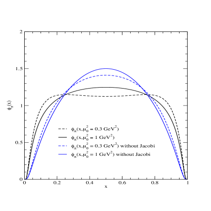
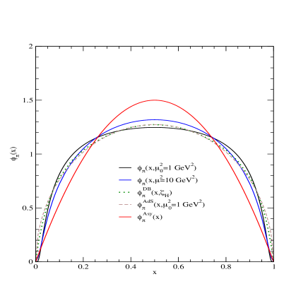
Figure 1: Left panel: Pion DAs with (black lines) and without (blue lines) the Jacobi factor at the scale $\mu^{2}_{0}=0.3$ GeV² (dashed lines) and $\mu^{2}_{0}=1$ GeV² (solid lines), respectively. Right panel: Pion DAs at initial scale $\mu^{2}_{0}=1$ GeV² (solid black line), which is evolved to $\mu^{2}=10$ GeV² (solid blue line).

In our recent works Jafar1 ; Jafar2 , we established the method to obtain the pseudoscalar meson decay constant within our standard LFQM in a process-independent and current component-independent manner. To provide a comprehensive understanding, we present here the essential aspect required to attain the Lorentz and rotational invariant result within our LFQM framework.

The pion decay constant defined by the local operator with axial vector, $\langle 0|{\bar{q}}(0)\gamma^{\mu}\gamma_{5}q(0)|\pi(P)\rangle=if_{\pi}P^{\mu}$, can be obtained as

$$f_{\pi} = \sqrt{N_{c}}\int_{0}^{1}{\rm d}x\int\frac{{\rm d}^{2}\mathbf{k}_{\bot}}{16\pi^{3}}\ \phi(x,\mathbf{k}_{\perp})$$ (10)

$$\times\mbox{}\frac{1}{iP^{\mu}}\sum_{\lambda_{1},\lambda_{2}}{\cal R}_{\lambda_{1}\lambda_{2}}\left[\frac{\bar{v}_{\lambda_{2}}(p_{2})}{\sqrt{x_{2}}}\gamma^{\mu}\gamma_{5}\frac{u_{\lambda_{1}}(p_{1})}{\sqrt{x_{1}}}\right],\;$$

where $N_{c}=3$ arises from the color factor implicit in the wave function. The final result of $f_{\pi}$ in the most general ${\bf P}_{\perp}\neq 0$ frame is given as follows Jafar2

$$f^{(\mu)}_{\pi}=\sqrt{2N_{c}}\int_{0}^{1}{\rm d}x\int\frac{{\rm d}^{2}\mathbf{k}_{\bot}}{16\pi^{3}}\ \frac{{\phi}(x,\mathbf{k}_{\bot})}{\sqrt{m^{2}+\mathbf{k}_{\bot}^{2}}}~{}\mathcal{O}^{(\mu)}_{\rm A}(x,{\bf k}_{\perp}),\;\;$$ (11)

where the operators ${\cal O}^{(\mu)}_{\rm A}$ derived from the currents with $\mu=(+,\perp)$ yield identical results, specifically ${\cal O}^{(+)}_{\rm A}={\cal O}^{(\perp)}_{\rm A}=2m$. For the minus component of the current, when the pion mass $M$ is employed in the Lorentz factor $P^{-}=(M^{2}+{\bf P}^{2}_{\perp})/P^{+}$, the result for ${\cal O}^{(-)}_{\rm A}$ is ${\cal O}^{(-)}_{\rm A}=2m(M^{2}_{0}+{\bf P}^{2}_{\perp})/(M^{2}+{\bf P}^{2}_{\perp})$. However, it is noteworthy that ${\cal O}^{(-)}_{\rm A}$ converges to the results obtained for $\mu=(+,\perp)$, specifically ${\cal O}^{(-)}_{\rm A}\to 2m$, when the substitution $M\to M_{0}$ is applied Jafar2 for the meson-quark vertex. More detailed analysis of the decay constant including the unequal quark and antiquark mass case can also be found in Jafar2 .

In particular, the pion DA $\phi_{\pi}(x)$ is completely independent of the current components and is given by

$$\phi_{\pi}(x,\mu_{0})=\frac{\sqrt{2N_{c}}}{f_{\pi}}\int^{\mu^{2}_{0}}\frac{{\rm d}^{2}\mathbf{k}_{\bot}}{16\pi^{3}}\ \frac{2m}{\sqrt{m^{2}+\mathbf{k}_{\bot}^{2}}}~{}{\phi}(x,\mathbf{k}_{\bot}),$$ (12)

where the normalization is fixed by $\int^{1}_{0}dx\phi_{\pi}(x,\mu_{0})=1$ at any scale $\mu_{0}$. The DA provides information about the probability amplitudes of finding the hadron in a state characterized by the minimum number of Fock constituents and small transverse-momentum separation. This is defined by an ultraviolet (UV) cutoff $\mu_{0}\geq 1$ GeV. The dependence on the scale is then given by the QCD evolution equation BL80 and can be calculated perturbatively. Nevertheless, the DA at a specific low scale can be determined by incorporating essential nonperturbative information from the LFQM. Additionally, the Gaussian wave function in our LFQM enables the accurate integration up to infinity without any loss of precision. For the nonperturbative valence wave function given by Eq. (8), we take $\mu_{0}=1$ GeV as an optimal scale for our LFQM.

To compare the leading-twist pion DA with high-energy experimental data, it is necessary to incorporate radiative logarithmic corrections through QCD evolution LB79 ; ER80 . The evolution of the pion DA at large $Q$ is governed by the Efremov-Radyushkin-Brodsky-Lepage (ERBL) equation. The solution of the ERBL equation can be expressed LB79 ; ER80 ; Muller95 ; AB02 in terms of Gegenbauer polynomials

$$\phi_{\pi}(x,\mu)=6x(1-x)\sum_{n=0}^{\infty}{}^{{}^{\prime}}C^{3/2}_{n}(2x-1)a_{n}(\mu),$$ (13)

where $C^{3/2}_{n}$ is the Gegenbauer polynomials of order $3/2$ and the prime indicates summation over even values of $n$ only. The matrix elements, $a_{n}(\mu)$, are the Gegenbauer moments given by

$$a_{n}(\mu) = \frac{2(2n+3)}{3(n+1)(n+2)}\left(\frac{\alpha_{s}(\mu)}{\alpha_{s}(\mu_{0})}\right)^{\frac{\gamma_{n}^{(0)}}{2\beta_{0}}}$$ (14)

$$\times\int^{1}_{0}dx\;C^{3/2}_{n}(2x-1)\phi_{\pi}(x,\mu_{0}),$$

where the strong coupling constant $\alpha_{s}(\mu)$ is given by

$$\alpha_{s}(\mu)=\frac{4\pi}{\beta_{0}\ln\left(\frac{\mu^{2}}{\Lambda^{2}_{\rm QCD}}\right)},$$ (15)

and

$$\gamma^{(0)}_{n} = -2C_{F}\left[3+\frac{2}{(n+1)(n+2)}-4\sum_{k=1}^{n+1}\frac{1}{k}\right],$$

$$\beta_{0} = 11-\frac{2}{3}N_{F},$$ (16)

with $N_{F}$ being the number of active flavors. We take here $N_{F}=3$. In the chiral limit (i.e. $m\to 0$) within our LFQM, we obtain $\phi^{\rm chiral}_{\pi}(x,\mu_{0})=1$. In this case, one gets $\int^{1}_{0}dx\;C^{3/2}_{n}(2x-1)\phi^{\rm chiral}_{\pi}(x,\mu_{0})=1$.

In the left panel of Fig. 1, we compare the pion DAs $\phi_{\pi}(x,\mu_{0})$ with (black lines) and without (blue lines) the Jacobi factor $\sqrt{\partial k_{z}/\partial x}$ in defining the radial wave function $\phi(x,{\bf k}_{\perp})$ given by Eq. (8). The solid and dashed lines are the results at the scales, $\mu^{2}_{0}=1$ and 0.3 GeV², respectively. There are a few points worth mentioning regarding the impact of the Jacobi factor on the LF wave function and DA of the pion: (1) The Jacobi factor plays a crucial role in preserving the Lorentz and rotation invariance of the decay constant Jafar1 ; Jafar2 . (2) The Jacobi factor flattens the shape of the DA at the midpoint of $x$ while amplifying the DA at the extreme points of $x=0$ and 1, in comparison to the outcome obtained without considering it. (3) The sensitivity of the cut-off scale $\mu_{0}$ is more pronounced in the outcome of $\phi_{\pi}(x)$ when incorporating the Jacobi factor, as compared to the result obtained without considering the Jacobi factor. In particular, when the Jacobi factor is included, the shape of the result undergoes a transformation from concave at the center of $x$ for $\mu_{0}<0.5$ GeV to convex for $\mu_{0}>0.5$ GeV. On the other hand, in the absence of the Jacobi factor, the shape remains convex regardless of the chosen scale $\mu_{0}$. In the right panel of Fig. 1, we show the pion DA at the initial scale $\mu^{2}_{0}=1$ GeV² (solid black line), which is evolved to $\mu^{2}=10$ GeV² (solid blue line) when we use Eq. (8) for the radial wave function. We also compare our results with the asymptotic result $\phi^{\rm Asy}=6x(1-x)$ (solid red line), the AdS/CFT prediction AdS1 ; AdS2 ; AdS3 $\phi^{\rm AdS}=\pi\sqrt{x(1-x)}/8$ (dashed line), and the result of Dyson-Schwinger equations (DSEs) DSE1 ; DSE2 ; DSE3 $\phi_{\rm DB}(x,\zeta_{\rm H})=20.227x(1-x)[1-2.5088\sqrt{x(1-x)}+2.0250x(1-x)]$ (dotted line) obtained from the dynamical-chiral-symmetry breaking-improved (DB) truncations at the scale $\zeta_{\rm H}=0.30$ GeV, respectively.

III Pion form factor

In this section, we first discuss the overarching framework that governs the transition between two pseudoscalar mesons, namely the transition from a pseudoscalar meson characterized by momentum $P$ and mass $M$ to another pseudoscalar meson with momentum $P^{\prime}$ and mass $M^{\prime}$. In this transition, the four-momentum transfer $q$ is introduced and defined as $q=P-P^{\prime}$. The general covariant decomposition of the matrix element for this transition, ${\cal J}^{\mu}\equiv\langle P^{\prime}|\bar{q}\gamma^{\mu}q|P\rangle$, is given by

$${\cal J}^{\mu} = \left[(P+P^{\prime})^{\mu}-q^{\mu}\frac{(M^{2}-M^{\prime 2})}{q^{2}}\right]F(q^{2})$$ (17)

$$+q^{\mu}\frac{(M^{2}-M^{\prime 2})}{q^{2}}H(q^{2}),$$

where the Lorentz structure containing the form factor $F(q^{2})$ is manifestly gauge invariant while the additional amplitude for $M\neq M^{\prime}$ as in the case of the weak decay is described by the form factor $H(q^{2})$. For the semileptonic decays between two different pseudoscalar mesons, $F(q^{2})$ and $H(q^{2})$ correspond to the weak form factors $f_{+}(q^{2})$ and $f_{0}(q^{2})$ related to the exchange of $1^{-}$ and $0^{+}$, respectively. The self-consistent treatment of the weak form factors $f_{+}(q^{2})$ and $f_{0}(q^{2})$ within the framework of the LFQM, employing the “type II” link that connects the covariant BS model to the LFQM, has been elaborated in Refs. Choi21 ; ChoiAdv .

In the case of the electromagnetic form factor of a pseudoscalar meson, the Lorentz structure proportional to $q^{\mu}$ associated with $H(q^{2})$ in Eq. (17) does not contribute to ${\cal J}^{\mu}$ due to the invariance of time reversal symmetry and only the gauge invariant form factor $F(q^{2})$ remains relevant, i.e.,

$${\cal J}^{\mu}_{\rm em} \equiv {\cal P}^{\mu}F_{\rm em}(q^{2})$$ (18)

$$= \left[(P+P^{\prime})^{\mu}-q^{\mu}\frac{(M^{2}-M^{\prime 2})}{q^{2}}\right]F_{\rm em}(q^{2}).$$

In Eq. (18), it is important to note the presence of the second term proportional to $(M^{2}-M^{\prime 2})$ on the right-hand side, which allows the electromagnetic gauge invariance $q\cdot{\cal J}_{\rm em}=0$ even if $M\neq M^{\prime}$. Of course, this term becomes zero when applying the physical mass relation, i.e., $M^{2}=M^{\prime 2}$. However, as discussed in the introduction, the consistent BT treatment of the noninteracting $q\bar{q}$ representation (i.e., $M^{(\prime)}\to M^{(\prime)}_{0}$) both in the matrix element ${\cal J}^{\mu}_{\rm em}$ and the Lorentz structure ${\cal P}^{\mu}\equiv(P+P^{\prime})^{\mu}-q^{\mu}({M_{0}}^{2}-{M^{\prime}_{0}}^{2})/q^{2}$ on the right-hand side of Eq. (18) is crucial in the LFQM computation based on the principles of the BT construction to obtain the physical observable $F_{\rm em}(q^{2})$ uniquely independent of the current components. The selective application of the noninteracting $q\bar{q}$ representation only to the matrix element ${\cal J}^{\mu}_{\rm em}$ but not to the Lorentz structure ${\cal P}^{\mu}$ may lead to the LF zero mode issue, particularly when dealing with the minus component ($\mu=-$) of the current.

In our self-consistent LFQM based on the BT construction where $M\to M_{0}$ and $M^{\prime}\to M^{\prime}_{0}$, we demonstrate that the second term proportional to $q^{\mu}$ in Eq. (18) is essential. It serves a dual purpose, enabling us to derive the current-component independent pion form factor and maintaining gauge invariance, specifically ensuring $q\cdot{\cal J}_{\rm em}=0$ even when replacing the physical mass $M^{(\prime)}$ with the invariant mass $M^{(\prime)}_{0}$.

Table 1: Helicity non-flip $h^{\mu}_{(\uparrow\to\uparrow)+(\downarrow\to\downarrow)}\equiv\sum_{{\bar{\lambda}}}(h^{\mu}_{\uparrow{\bar{\lambda}}\to\uparrow{\bar{\lambda}}}+h^{\mu}_{\downarrow{\bar{\lambda}}\to\downarrow{\bar{\lambda}}})$ and the helicity flip $h^{\mu}_{(\uparrow\to\downarrow)+(\downarrow\to\uparrow)}\equiv\sum_{{\bar{\lambda}}}(h^{\mu}_{\uparrow{\bar{\lambda}}\to\downarrow{\bar{\lambda}}}+h^{\mu}_{\downarrow{\bar{\lambda}}\to\uparrow{\bar{\lambda}}})$ contributions from the spin trace term and the Lorentz factor ${\cal P}^{\mu}$ obtained from each component of the currents ${\cal J}^{\mu}_{\rm em}$

. Current components $h^{\mu}_{(\uparrow\to\uparrow)+(\downarrow\to\downarrow)}$ $h^{\mu}_{(\uparrow\to\downarrow)+(\downarrow\to\uparrow)}$ ${\cal P}^{\mu}$ ${\cal J}^{+}_{\rm em}$ $\frac{2(m^{2}+{\bf k}_{\perp}\cdot{\bf k}^{\prime}_{\perp})}{\sqrt{m^{2}+{\bf k}^{2}_{\perp}}\sqrt{m^{2}+{\bf k}^{\prime 2}_{\perp}}}$ 0 $2P^{+}$ ${\bf{\cal J}}^{\perp}_{\rm em}$ $-\frac{(m^{2}+{\bf k}_{\perp}\cdot{\bf k}^{\prime}_{\perp})({\bf q}_{\perp}+2{\bf k}_{\perp})}{xP^{+}\sqrt{m^{2}+{\bf k}^{2}_{\perp}}\sqrt{m^{2}+{\bf k}^{\prime 2}_{\perp}}}$ 0 $-{\bf q}_{\perp}\left(1-\frac{M^{2}_{0}-M^{\prime 2}_{0}}{{\bf q}^{2}_{\perp}}\right)$ ${\cal J}^{-}_{\rm em}$ $\frac{2m^{2}(1-x){\bf q}^{2}_{\perp}}{x^{2}(P^{+})^{2}\sqrt{m^{2}+{\bf k}^{2}_{\perp}}\sqrt{m^{2}+{\bf k}^{\prime 2}_{\perp}}}$ $\frac{2({\bf k}_{\perp}\cdot{\bf k}^{\prime}_{\perp}+m^{2})({\bf k}^{2}_{\perp}+{\bf k}_{\perp}\cdot{\bf q}_{\perp}+m^{2})+(1-x)({\bf k}_{\perp}\times{\bf q}_{\perp})^{2}}{x^{2}(P^{+})^{2}\sqrt{m^{2}+{\bf k}^{2}_{\perp}}\sqrt{m^{2}+{\bf k}^{\prime 2}_{\perp}}}$ $\frac{2M^{\prime 2}_{0}{\bf q}^{2}_{\perp}+{\bf q}^{4}_{\perp}+(M^{2}_{0}-M^{\prime 2}_{0})^{2}}{{\bf q}^{2}_{\perp}P^{+}}$

Table 2: The operators ${\cal O}^{(\mu)}_{\rm LFQM}$ and their helicity contributions to the pion form factor in the standard LFQM.

$F^{(\mu)}_{\pi}$	${\cal O}^{(\mu)}_{\rm LFQM}$	${\cal H}^{(\mu)}_{(\uparrow\to\uparrow)+(\downarrow\to\downarrow)}$	${\cal H}^{(\mu)}_{(\uparrow\to\downarrow)+(\downarrow\to\uparrow)}$
$F^{(+)}_{\pi}$	${\bf k}_{\perp}\cdot{\bf k}^{\prime}_{\perp}+m^{2}$	${\bf k}_{\perp}\cdot{\bf k}^{\prime}_{\perp}+m^{2}$	0
$F^{(\perp)}_{\pi}$	${\bf k}_{\perp}\cdot{\bf k}^{\prime}_{\perp}+m^{2}$	${\bf k}_{\perp}\cdot{\bf k}^{\prime}_{\perp}+m^{2}$	0
$F^{(-)}_{\pi}$	$\frac{2(1-x){\bf q}^{2}_{\perp}M^{2}_{0}({\bf k}_{\perp}\cdot{\bf k}^{\prime}_{\perp}+m^{2}+{\bf q}_{\perp}\cdot{\bf k}^{\prime}_{\perp})}{x[2M^{\prime 2}_{0}{\bf q}^{2}_{\perp}+{\bf q}^{4}_{\perp}+(M^{2}_{0}-M^{\prime 2}_{0})^{2}]}$	$\frac{2{\bf q}^{2}_{\perp}\{({\bf k}_{\perp}\cdot{\bf k}^{\prime}_{\perp}+m^{2})({\bf k}^{2}_{\perp}+{\bf k}_{\perp}\cdot{\bf q}_{\perp}+m^{2})+(1-x)({\bf k}_{\perp}\times{\bf q}_{\perp})^{2}\}}{x^{2}[2M^{\prime 2}_{0}{\bf q}^{2}_{\perp}+{\bf q}^{4}_{\perp}+(M^{2}_{0}-M^{\prime 2}_{0})^{2}]}$	$\frac{2{\bf q}^{2}_{\perp}\{(1-x)m^{2}{\bf q}^{2}_{\perp}\}}{x^{2}[2M^{\prime 2}_{0}{\bf q}^{2}_{\perp}+{\bf q}^{4}_{\perp}+(M^{2}_{0}-M^{\prime 2}_{0})^{2}]}$

To compute the pion form factor defined in Eq. (18), we use the Drell-Yan-West ($q^{+}=0$) frame with ${\bf P}_{\perp}=0$, where $q^{2}=-{\bf q}^{2}_{\perp}\equiv-Q^{2}$. In this frame, we have

$$P=\left(P^{+},\frac{M^{2}}{P^{+}},0_{\perp}\right),\;P^{\prime}=\left(P^{+},\frac{M^{\prime 2}+{\bf q}^{2}_{\perp}}{P^{+}},-{\bf q}_{\perp}\right),$$

$$q=\left(0,\frac{M^{2}-M^{\prime 2}-{\bf q}^{2}_{\perp}}{P^{+}},{\bf q}_{\perp}\right).$$ (19)

For $P(q_{1}{\bar{q}})\to P^{\prime}(q_{2}{\bar{q}})$ transition with the momentum transfer $q=P-P^{\prime}$, the relevant on-mass shell quark momentum variables in the $q^{+}=0$ frame are given by

$$p^{+}_{1}=xP^{+},\;p^{+}_{\bar{q}}=(1-x)P^{+},$$

$${\bf p}_{1\perp}=x{\bf P}_{\perp}-{\bf k}_{\perp},\;{\bf p}_{{\bar{q}}\perp}=(1-x){\bf P}_{\perp}+{\bf k}_{\perp},$$

$$p^{+}_{2}=xP^{+},\;p^{\prime+}_{\bar{q}}=(1-x)P^{+},$$

$${\bf p}_{2\perp}=x{\bf P}^{\prime}_{\perp}-{\bf k}^{\prime}_{\perp},\;{\bf p}^{\prime}_{{\bar{q}}\perp}=(1-x){\bf P}^{\prime}_{\perp}+{\bf k}^{\prime}_{\perp}.$$ (20)

Since the spectator quark (${\bar{q}}$) requires that $p^{+}_{\bar{q}}=p^{\prime+}_{\bar{q}}$ and ${\bf p}_{{\bar{q}}\perp}={\bf p}^{\prime}_{{\bar{q}}\perp}$, one obtains ${\bf k}^{\prime}_{\perp}={\bf k}_{\perp}+(1-x){\bf q}_{\perp}$.

The matrix element ${\cal J}^{\mu}_{\rm em}=\langle\pi(P^{\prime})|\bar{q}\gamma^{\mu}q|\pi(P)\rangle$ in the one-loop contribution within the framework of the LFQM based on the noninteracting $q{\bar{q}}$ representation consistent with the BT construction is then obtained by the convolution of the initial and final state LF wave functions as follows:

$${\cal J}^{\mu}_{\rm em} = \int^{1}_{0}dp^{+}_{1}\int\frac{d^{2}\mathbf{k}_{\bot}}{16\pi^{3}}\ \phi^{\prime}(x,\mathbf{k}^{\prime}_{\perp})\phi(x,\mathbf{k}_{\perp})\sum_{\lambda^{\prime}s}h^{\mu}_{\lambda_{1}{\bar{\lambda}}\to\lambda_{2}{\bar{\lambda}}},$$ (21)

$$= \int^{1}_{0}dp^{+}_{1}\int\frac{d^{2}\mathbf{k}_{\bot}}{16\pi^{3}}\ \phi^{\prime}(x,\mathbf{k}^{\prime}_{\perp})\phi(x,\mathbf{k}_{\perp})$$

$$\hskip 34.14322pt\times\;\left[h^{\mu}_{(\uparrow\to\uparrow)+(\downarrow\to\downarrow)}+h^{\mu}_{(\uparrow\to\downarrow)+(\downarrow\to\uparrow)}\right],$$

where

$$h^{\mu}_{\lambda_{1}{\bar{\lambda}}\to\lambda_{2}{\bar{\lambda}}}\equiv\mathcal{R}^{\dagger}_{\lambda_{2}{\bar{\lambda}}}\left[\frac{\bar{u}_{\lambda_{2}}(p_{2})}{\sqrt{p^{+}_{2}}}\gamma^{\mu}\frac{u_{\lambda_{1}}(p_{1})}{\sqrt{p^{+}_{1}}}\right]\mathcal{R}_{\lambda_{1}{\bar{\lambda}}}$$ (22)

is the term of spin trace, and $h^{\mu}_{(\uparrow\to\uparrow)+(\downarrow\to\downarrow)}\equiv\sum_{{\bar{\lambda}}}(h^{\mu}_{\uparrow{\bar{\lambda}}\to\uparrow{\bar{\lambda}}}+h^{\mu}_{\downarrow{\bar{\lambda}}\to\downarrow{\bar{\lambda}}})$ and $h^{\mu}_{(\uparrow\to\downarrow)+(\downarrow\to\uparrow)}\equiv\sum_{{\bar{\lambda}}}(h^{\mu}_{\uparrow{\bar{\lambda}}\to\downarrow{\bar{\lambda}}}+h^{\mu}_{\downarrow{\bar{\lambda}}\to\uparrow{\bar{\lambda}}})$ are the helicity non-flip and the helicity flip contributions, respectively.

Now, applying the same BT construction to the Lorentz factor ${\cal P}^{\mu}$ in Eq. (18), we obtain the pion form factor $F^{(\mu)}_{\pi}$ for any component ($\mu=+,-,\perp$) of the current as

$$F^{(\mu)}_{\pi}(Q^{2}) = \int^{1}_{0}dp^{+}_{1}\int\frac{{\rm d}^{2}\mathbf{k}_{\bot}}{16\pi^{3}}\ \phi^{\prime}(x,\mathbf{k}^{\prime}_{\perp})\phi(x,\mathbf{k}_{\perp})$$

$$\hskip 28.45274pt\times\;\frac{\left[h^{\mu}_{(\uparrow\to\uparrow)+(\downarrow\to\downarrow)}+h^{\mu}_{(\uparrow\to\downarrow)+(\downarrow\to\uparrow)}\right]}{\cal P^{\mu}}.\;\;$$

It is important to note that all meson mass terms, denoted as $M^{(\prime)}$, appearing in ${\cal P}^{\mu}$ are substituted with $M^{(\prime)}_{0}$, where $M^{\prime}_{0}=M_{0}({\bf k}_{\perp}\rightarrow{\bf k}^{\prime}_{\perp})$ represents the invariant mass of the final state pion.

The helicity non-flip $h^{\mu}_{(\uparrow\to\uparrow)+(\downarrow\to\downarrow)}$ and the helicity flip $h^{\mu}_{(\uparrow\to\downarrow)+(\downarrow\to\uparrow)}$ contributions from the spin trace term together with the Lorentz factor ${\cal P}^{\mu}$ obtained from each component of the current ${\cal J}^{\mu}_{\rm em}$ are summarized in Table 1. We note that the $\mu=+$ and $\perp$ components of the current ${\cal J}^{\mu}_{\rm em}$ receive only the helicity non-flip contributions. On the other hand, the minus ($\mu=-$) component of the current receives both the helicity non-flip and helicity flip contributions. Detailed derivation of helicity contributions for each current component is presented in the Appendix A.

From Table 1, we now obtain the pion form factor for each component of the current ${\cal J}^{\mu}_{\rm em}$ as follows:

$$F^{(\mu)}_{\pi}(Q^{2})=\int^{1}_{0}dx\int\frac{d^{2}{\bf k}_{\perp}}{16\pi^{3}}\frac{\phi(x,{\bf k}_{\perp})\phi^{\prime}(x,{\bf k}^{\prime}_{\perp})}{\sqrt{m^{2}+{\bf k}^{2}_{\perp}}\sqrt{m^{2}+{\bf k}^{\prime 2}_{\perp}}}{\cal O}^{(\mu)}_{\rm LFQM}.$$ (24)

Here, the operators ${\cal O}^{(\mu)}_{\rm LFQM}$ are obtained from the expression $\frac{h^{\mu}_{(\uparrow\to\uparrow)+(\downarrow\to\downarrow)}+h^{\mu}_{(\uparrow\to\downarrow)+(\downarrow\to\uparrow)}}{\cal P^{\mu}}$ in Eq. (III). This process involves isolating the common denominator factor, ${\cal K}\equiv\sqrt{m^{2}+{\bf k}^{2}_{\perp}}\sqrt{m^{2}+{\bf k}^{\prime 2}_{\perp}}$, and incorporating it into the wave functions. Consequently, we define ${\cal O}^{(\mu)}_{\rm LFQM}$ as follows:

$${\cal O}^{(\mu)}_{\rm LFQM} = {\cal K}P^{+}\frac{\left[h^{\mu}_{(\uparrow\to\uparrow)+(\downarrow\to\downarrow)}+h^{\mu}_{(\uparrow\to\downarrow)+(\downarrow\to\uparrow)}\right]}{\cal P^{\mu}}$$ (25)

$$\equiv {\cal H}^{(\mu)}_{(\uparrow\to\uparrow)+(\downarrow\to\downarrow)}+{\cal H}^{\mu}_{(\uparrow\to\downarrow)+(\downarrow\to\uparrow)}\;,$$

where $P^{+}$ comes from the transformation of $dp^{+}_{1}=P^{+}dx$ in Eq. (III).

In Table 2, we provide a summary of the results for ${\cal O}^{(\mu)}_{\rm LFQM}$, along with the contributions from helicity non-flip and flip processes, denoted as ${\cal H}^{(\mu)}_{(\uparrow\to\uparrow)+(\downarrow\to\downarrow)}$ and ${\cal H}^{(\mu)}_{(\uparrow\to\downarrow)+(\downarrow\to\uparrow)}$, respectively. These results are presented for each component $(\mu=\pm,\perp)$ of the current.

As evident from Table 2, the pion form factor $F^{(+)}_{\pi}$ obtained from the plus current exhibits precisely the same analytical form as the form factor $F^{(\perp)}_{\pi}$ derived from the perpendicular current. Furthermore, both form factors exclusively receive contributions related to helicity non-flip processes, and are not affected by zero-mode contributions as discussed in Ref. CJ15 . In contrast, the form factor obtained from the minus component of the current encompasses not only the helicity non-flip but also the helicity flip contributions. Taking into account both the helicity non-flip and flip contributions for $F^{(-)}_{\pi}$, we have found that all three form factors yield numerically identical results, indicating $F^{(+)}_{\pi}=F^{(\perp)}_{\pi}=F^{(-)}_{\pi}$. It is remarkable that we achieved obtaining the physical observable $F_{\rm em}(q^{2})$ as independent of the current components.

In Appendix B, we present a detailed derivation of Eq. (24) starting from the covariant BS model and applying the “type II” link, as exemplified in Eq. (49) of CJ14 , which establishes a connection between the covariant BS model and the LFQM. As explained in Appendix B, it is noteworthy that in the ${\bf{\cal J}}^{\perp}_{\rm em}$ case, the same form factor $F^{(\perp)}_{\pi}$ is obtained even when using the traditional Lorentz factor $(P+P^{\prime})^{\mu}$ without incorporating the term proportional to $q^{\mu}$. This suggests that using $(P+P^{\prime})^{\mu}$ yields the correct pion form factor when utilizing the $\mu=\perp$ components of the current as in the case of utilizing the $\mu=+$ component of the current. This observation implies that the form factor derived from the $({\cal J^{+}_{\rm em}},{\bf{\cal J}}^{\perp}_{\rm em})$ currents is devoid of LF zero modes. On the contrary, the pion form factor $F^{(-)}_{\pi}$ derived from the ${\cal J}^{-}_{\rm em}$ current using the traditional Lorentz factor $(P+P^{\prime})^{\mu}$ yields notably different results, deviating from the exact solution $F^{(+)}_{\pi}=F^{(\perp)}_{\pi}$. This disparity is typically attributed to the LF zero-mode contribution to $F^{(-)}_{\pi}$. Consequently, our method for obtaining the exact result for $F^{(-)}_{\pi}$ with the ${\bf{\cal J}}^{-}_{\rm em}$ current, as presented in Table 2 and utilizing the Lorentz factor ${\cal P}^{\mu}$ consistently with the BT construction for the valence picture of LFQM, indicates an effective inclusion of the LF zero mode associated with the nonvalence contribution from higher Fock states.

In Appendix C, we also present our numerical results for the pion form factor and investigate the influence of the quark running mass, treating it exclusively as a function of the momentum transfer $Q^{2}$.

IV TMD and PDF of Pion

In Refs. Lorce ; LPS16 , the authors established the formalism to describe unpolarized higher-twist TMDs within the LFQM framework of constituent quarks, on par with the other interacting models such as the spectator Jakob , chiral quark-soliton Schw03 , and bag Bag models. Focusing on unpolarized targets within the framework of quark models, the authors presented the 4 TMDs as the complete set of unpolarized T-even TMDs. They also derived the Lorentz-invariance relation among unpolarized TMDs, which is valid in the framework of quark models without explicit gauge degrees of freedom. Among those 4 TMDs, which are expressed in terms of hadronic matrix elements of bilinear quark-field correlators of the type $\langle h|{\bar{\psi}}(0)\Gamma\psi(z)|h\rangle$, three of them are essentially related with the forward matrix elements of the electromagnetic form factor, i.e. $\langle h|{\bar{\psi}}(0)\gamma^{\mu}\psi(0)|h\rangle$ with $\mu=+,-,\perp$, and the remaining one is related with the matrix element of the unit operator $\Gamma=\mathbf{1}$.

The LFQM utilized in  Lorce ; LPS16 shares similarities with ours in that they both employ the constituent-quark picture in calculating matrix elements. However, a notable difference of ours stems from the BT construction consistently applied to both the meson-quark vertex and the Lorentz factor associated with the physical observable. Apparently, the authors of Refs. Lorce ; LPS16 noticed the difficulties encountered in computing the twist-4 quark TMD and PDF, denoted as $f^{q}_{4}(x,{\bf k}_{\perp})$ and $f^{q}_{4}(x)$, respectively. In particular, they attributed the reason why the sum rule for $f^{q}_{4}(x)$, i.e., $2\int dxf^{q}_{4}(x)=1$, was not satisfied to the issue of the nonvanishing LF zero mode. In this section, we provide the analysis of the three TMDs and PDFs related to the forward matrix elements $\langle h|\bar{\psi}(0)\gamma^{\mu}\psi(0)|h\rangle$, resolving the difficulties noticed in Refs. Lorce ; LPS16 . We discuss our effective resolution of the LF zero mode issue associated with the twist-4 TMD and PDF.

IV.1 TMD

TMDs are typically defined through quark correlators. In constituent models that lack explicit gluon degrees of freedom, the Wilson lines in QCD simplify to unit matrices in color space. Consequently, T-odd TMDs are not present, and only T-even TMDs are observable. The characterization of a spin-zero hadron, such as the pion, is achieved using four specific TMDs, as discussed in Refs. Lorce ; LPS16 . Three of four TMDs for pion are related with the forward matrix element $\langle P|{\bar{q}}\gamma^{\mu}q|P\rangle$ of the vector currents, which are defined as Lorce ; LPS16

$$\int\frac{[dz]}{2(2\pi)^{3}}e^{ip\cdot z}\langle P|{\bar{\psi}}(0)\gamma^{+}\psi(z)|P\rangle|_{z^{+}=0} =f^{q}_{1}(x,p_{T}),$$

$$\int\frac{[dz]}{2(2\pi)^{3}}e^{ip\cdot z}\langle P|{\bar{\psi}}(0)\gamma^{j}_{T}\psi(z)|P\rangle|_{z^{+}=0} =\frac{p^{j}_{T}}{P^{+}}f^{q}_{3}(x,p_{T}),$$

$$\int\frac{[dz]}{2(2\pi)^{3}}e^{ip\cdot z}\langle P|{\bar{\psi}}(0)\gamma^{-}\psi(z)|P\rangle|_{z^{+}=0} =\left(\frac{m_{\pi}}{P^{+}}\right)^{2}f^{q}_{4}(x,p_{T}),$$

where $[dz]=dz^{-}d^{2}z_{T}$, $|P\rangle$ denotes a pion state with four-momentum $P$, $q$ represents the flavor index for the quark and antiquark contributions, and $m_{\pi}$ stands for the pion mass. Additionally, $f^{q}_{1}(x,p_{T})$, $f^{q}_{3}(x,p_{T})$, and $f^{q}_{4}(x,p_{T})$ with $p_{T}=|{\bf p}_{T}|$ correspond to the unpolarized TMDs of twist-2, twist-3, and twist-4, respectively. While twist-4 TMDs are primarily of academic interest, it is worth noting that $f^{q}_{4}(x,p_{T})$ becomes intertwined with other twist-4 quark-gluon correlators, such as those associated with power corrections to the Deep Inelastic Scattering structure functions, as discussed in Lorce ; Jaffe83 ; Shuryak ; Jaffe81 ; Ellis83 ; Qui90 ; XJi93 ; Geyer .

Integrating out the right-hand side of Eq. (IV.1), one obtains

$$\int\frac{[dz]}{2(2\pi)^{3}}e^{ip\cdot z}\langle P|{\bar{\psi}}(0)\gamma^{\mu}\psi(z)|P\rangle$$

$$=\int\frac{dz^{-}}{4\pi}e^{ixP^{+}z^{-}}\langle P|{\bar{\psi}}(0)\gamma^{\mu}\psi(z^{-})|P\rangle$$

$$=\int\frac{dz^{-}}{4\pi}e^{i(xP^{+}-p^{+})z^{-}}\langle P|{\bar{\psi}}(0)\gamma^{\mu}\psi(0)|P\rangle$$

$$=\frac{\delta(x-p^{+}/P^{+})}{2P^{+}}\langle P|{\bar{\psi}}(0)\gamma^{\mu}\psi(0)|P\rangle,$$ (27)

where $\psi(z)|_{z^{+}=z_{T}=0}\equiv\psi(z^{-})$. We should note here that we adopted the same metric convention as used in Lorce ; LPS16 , $a\cdot b=a^{+}b^{-}+a^{-}b^{+}-a_{T}\cdot b_{T}$, when deriving Eq. (IV.1) for the consistency with the definitions of TMDs as outlined in Lorce ; LPS16 . Consequently, following this definition as discussed in Lorce ; LPS16 , one has $2P^{+}P^{-}=m^{2}_{\pi}$.

Using the relation in Eq. (IV.1), Eq. (IV.1) can be rewritten as follows

$$2P^{+}\int dxf^{q}_{1}(x) = \langle P|{\bar{\psi}}(0)\gamma^{+}\psi(0)|P\rangle,$$

$$2p_{T}\int dxf^{q}_{3}(x) = \langle P|{\bar{\psi}}(0)\gamma^{\perp}\psi(0)|P\rangle,$$

$$4P^{-}\int dxf^{q}_{4}(x) = \langle P|{\bar{\psi}}(0)\gamma^{-}\psi(0)|P\rangle,$$ (28)

where the functions $f(x)=\{f^{q}_{1}(x),f^{q}_{3}(x),f^{q}_{4}(x)\}$ represent the PDFs obtained through the integration of the corresponding TMDs $f(x,p_{T})=\{f^{q}_{1}(x,p_{T}),f^{q}_{3}(x,p_{T}),f^{q}_{4}(x,p_{T})\}$ over $p_{T}$, and this integration is expressed as follows:

$$f(x)=\int d^{2}p_{T}f(x,p_{T}).$$ (29)

As discussed in Lorce ; LPS16 , it is important to note that, due to the explicit $p_{T}$ factor in Eq. (IV.1), there is no direct PDF counterpart to the twist-3 TMD, $f^{q}_{3}(x,p_{T})$. However, it is possible to formally define $f^{q}_{3}(x)$ as presented in Eq. (29).

The authors in Lorce ; LPS16 utilized the forward matrix elements, expressed as $\langle P|J^{q}_{\mu}|P\rangle=2P_{\mu}F^{q}(0)$, with $F^{q}(0)=1$. In other words, they employed the traditional Lorentz factor ${\cal\tilde{P}}^{\mu}\equiv\lim_{Q^{2}\to 0}(P+P^{\prime})^{\mu}=2P^{\mu}$ at the $Q^{2}\to 0$ limit and derived the sum rules for $f^{q}_{1}(x)$ and $f^{q}_{4}(x)$ from Eq. (IV.1) as:

$$2\int dxf^{q}_{4}(x) =\int dxf^{q}_{1}(x)=1,$$ (30)

along with establishing the relation between twist-2 and twist-3 TMDs as:

$$xf^{q}_{3}(x,p_{T}) =f^{q}_{1}(x,p_{T}).$$ (31)

Especially, the sum rules given by Eq. (30) implies that

$$\int dxf^{q}_{1}(x) = \frac{\langle P|J^{+}|P\rangle}{{\cal\tilde{P}}^{+}}=1,$$

$$2\int dxf^{q}_{4}(x) = \frac{\langle P|J^{-}|P\rangle}{{\cal\tilde{P}}^{-}}=1.$$ (32)

With the traditional Lorentz factor ${\cal\tilde{P}}^{\mu}$ employed in the forward matrix element, while the zeroth moment for $f^{q}_{1}(x)$ remains correct, the zeroth moment for $f^{q}_{4}(x)$ fails to satisfy Eq. (IV.1) due to the involvement of the LF zero mode arising from the minus component of the current. The similar complication encountered in the form factor calculation was discussed in Sec. III.

We note that the authors in LPS16 indeed computed the twist-4 PDF $f^{q}_{4}(x)$ using essentially the same LFQM with the model parameters, $(m,\beta)=(0.25,0.3194)$ GeV, but with the physical pion mass in $P^{-}$. Figure 2 shows $f^{q}_{4}(x)$ obtained from the method used in LPS16 , where we plot with two parameter sets, $(m,\beta)=(0.25,0.3194)$ GeV and (0.22, 0.3659) GeV, respectively. Numerically, we obtain

$$\int dxf^{q}_{4}(x) = 48.58\;{\rm for}\;m=0.25\;{\rm GeV},$$ (33)

$$= 66.45\;{\rm for}\;m=0.22\;{\rm GeV},$$

which are notably different from the expected value of 1/2. The authors of Lorce ; LPS16 attributed this discrepancy to inadequate estimation of the zero-mode contribution to the $J^{-}$ current in the computation of $f^{q}_{4}(x)$.

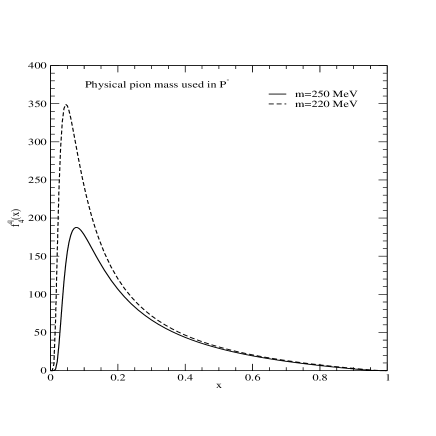
Figure 2: The twist-4 pion PDF, obtained using the methodology from LPS16 , while accounting the physical pion mass in $P^{-}$.

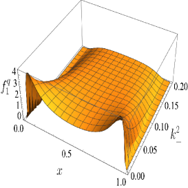
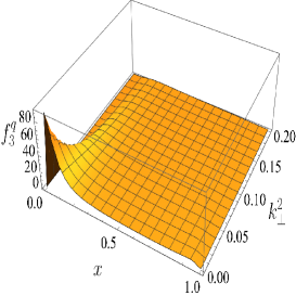
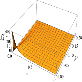
(a)                                         (b)                                         (c)

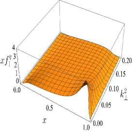
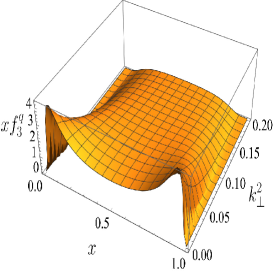
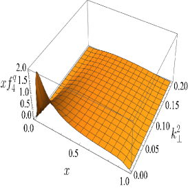
(d)                                         (e)                                         (f)

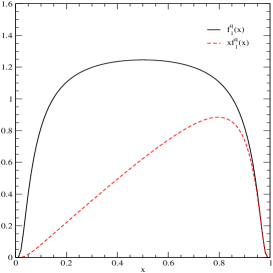
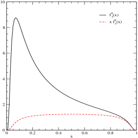
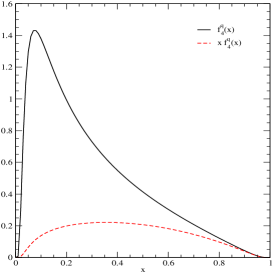
(g)                                         (h)                                         (i)

Figure 3: The unpolarized TMDs for pion, $f^{q}_{i}(x,{\bf k}_{\perp})$ (top panel) and $xf^{q}_{i}(x,{\bf k}_{\perp})(i=1,3,4)$ (middle panel), as a function of $x$ and ${\bf k}^{2}_{\perp}$, and the corresponding PDFs, $f^{q}_{i}(x)$ and $xf^{q}_{i}(x)$ (bottom panel) at the scale $\mu^{2}_{0}=1$ GeV².

In our LFQM, the matrix element $\langle P|{\bar{\psi}}(0)\gamma^{\mu}\psi(0)|P\rangle\equiv\langle P|J^{\mu}|P\rangle$ can be obtained from the forward limit ($Q^{2}\to 0$) of Eq. (21), i.e., $\lim_{Q^{2}\to 0}\langle P^{\prime}|J^{\mu}|P\rangle$ as follows

$$\langle P|J^{\mu}|P\rangle = \lim_{Q^{2}\to 0}\int dp^{+}_{1}\int\frac{{\rm d}^{2}\mathbf{k}_{\bot}}{16\pi^{3}}\ \phi^{\prime}(x,\mathbf{k}^{\prime}_{\perp})\phi(x,\mathbf{k}_{\perp})$$

$$\mbox{}\hskip 28.45274pt\times\left[h^{\mu}_{(\uparrow\to\uparrow)+(\downarrow\to\downarrow)}+h^{\mu}_{(\uparrow\to\downarrow)+(\downarrow\to\uparrow)}\right].$$

For the twist-2 TMD obtained from the $J^{+}$ current, one can easily find that $h^{+}_{(\uparrow\to\uparrow)+(\downarrow\to\downarrow)}(Q^{2}=0)=2$ and $h^{+}_{(\uparrow\to\downarrow)+(\downarrow\to\uparrow)}=0$ from Table 1 and thus obtain

$$\langle P|J^{+}|P\rangle=2P^{+}\int dx\int\frac{d^{2}\mathbf{k}_{\bot}}{16\pi^{3}}\ |\phi(x,\mathbf{k}_{\perp})|^{2}.$$ (35)

Comparing this with Eq. (IV.1), one can readily determine $f^{q}_{1}(x,{\bf k}_{\perp})$ as follows

$$f^{q}_{1}(x,{\bf k}_{\perp})=\frac{1}{16\pi^{3}}|\phi(x,\mathbf{k}_{\perp})|^{2},$$ (36)

where the twist-2 TMD and PDF satisfy the sum rule given by Eq. (30)

$$\int dx\int d^{2}{\bf k}_{\perp}f^{q}_{1}(x,{\bf k}_{\perp})=\int dxf^{q}_{1}(x)=1.$$ (37)

Likewise, by using Eq. (IV.1) and the results, $h^{\perp}_{(\uparrow\to\uparrow)+(\downarrow\to\downarrow)}(Q^{2}=0)$=$-\frac{2{\bf k}_{\perp}}{xP^{+}}$ and $h^{\perp}_{(\uparrow\to\downarrow)+(\downarrow\to\uparrow)}=0$ from Table 1, one can also find

$$\langle P|J^{\perp}|P\rangle=\int dx\int\frac{d^{2}\mathbf{k}_{\bot}}{16\pi^{3}}\ |\phi(x,\mathbf{k}_{\perp})|^{2}\left(-\frac{2{\bf k}_{\perp}}{x}\right).$$ (38)

Comparing this with Eq. (IV.1) and the formal definition of the twist-3 TMD given by Eq. (29), the twist-3 TMD in the LFQM can be extracted as

$$2{\bf k}_{\perp}f^{q}_{3}(x,{\bf k}_{\perp})=\frac{1}{16\pi^{3}}|\phi(x,\mathbf{k}_{\perp})|^{2}\left(-\frac{2{\bf k}_{\perp}}{x}\right),$$ (39)

that is, we obtain the relation

$$xf^{q}_{3}(x,{\bf k}_{\perp})=-f^{q}_{1}(x,{\bf k}_{\perp}).$$ (40)

While our result in Eq. (40) aligns with the relation provided by Eq. (31), there is a discrepancy in the overall sign. Specifically, following the definition of the twist-3 TMD in Eq. (IV.1), we find that $f^{q}_{3}(x,{\bf k}_{\perp})$ is negative ($f^{q}_{3}(x,{\bf k}_{\perp})\leq 0$), unlike the case of $f^{q}_{1}(x,{\bf k}_{\perp})$, which is positive ($f^{q}_{1}(x,{\bf k}_{\perp})\geq 0$). Therefore, to ensure the twist-3 TMD and PDF are positive, we need to adjust the overall sign in the definition of Eq. (IV.1). However, for the sake of the magnitude comparison modulo overall sign in our numerical calculation, we present our results for $f^{q}_{3}(x,{\bf k}_{\perp})$ and $f^{q}_{3}(x)$ as positive quantities.

Finally, to correctly account for the LF zero-mode contribution to the twist-4 TMD and PDF obtained from the $J^{-}$ current and to ensure adherence to the sum rule for $f^{q}_{4}(x)$ within the LFQM, we find that one should take the Lorentz factor as ${\cal P}^{\mu}=(P+P^{\prime})^{\mu}-q^{\mu}\frac{M^{2}-M^{\prime 2}}{q^{2}}$ not as the conventional ${\cal\tilde{P}}^{\mu}=(P+P^{\prime})^{\mu}$ and compute the normalization of the forward matrix element as previously discussed in Sec.III :

$$1=F(Q^{2}=0)=\lim_{Q^{2}\to 0}\langle P^{\prime}|\frac{J^{\mu}}{{\cal P}^{\mu}}|P\rangle.$$ (41)

This treatment achieves the current-component independent normalization of the pion form factor at $Q^{2}=0$ and necessitates consequently modifying the relation for $f^{q}_{4}(x)$ to satisfy the sum rule $2\int dxf^{q}_{4}(x)=1$ from Eq. (IV.1) to the modified relation given by:

$$\int dxf^{(-)}(x) = \lim_{Q^{2}\to 0}\langle P^{\prime}|\frac{J^{-}}{{\cal P}^{-}}|P\rangle=1,$$ (42)

where $f^{(-)}=2f^{q}_{4}(x)$ can be straightforwardly obtained from Eq. (III) as

$$f^{(-)}(x) = \int d^{2}{\bf k}_{\perp}f^{(-)}(x,{\bf k}^{2}_{\perp})$$

$$= \lim_{Q^{2}\to 0}\int\frac{{\rm d}^{2}\mathbf{k}_{\bot}}{16\pi^{3}}\ \phi^{\prime}(x,\mathbf{k}^{\prime}_{\perp})\phi(x,\mathbf{k}_{\perp})$$

$$\hskip 19.91684pt\times\;\frac{P^{+}\left[h^{-}_{(\uparrow\to\uparrow)+(\downarrow\to\downarrow)}+h^{-}_{(\uparrow\to\downarrow)+(\downarrow\to\uparrow)}\right]}{\cal P^{-}}.\;\;$$

Here, the unpolarized twist-4 TMD is defined as $2f^{q}_{4}(x,{\bf k}^{2}_{\perp})=f^{(-)}(x,{\bf k}^{2}_{\perp})$. We note in Eq. (IV.1) that the meson masses $M(M^{\prime})$ should be taken as the invariant masses $M_{0}(M^{\prime}_{0})$ in computing ${\cal P}^{-}$. This approach effectively resolves the LF zero mode issue of $f^{q}_{4}(x)$ satisfying the sum rule given by Eq. (30) correctly.

In Fig. 3, we show the unpolarized TMDs for pion up to twist-4, i.e., $f^{q}_{i}(x,{\bf k}_{\perp})$ (top panel) and $xf^{q}_{i}(x,{\bf k}_{\perp})(i=1,3,4)$ (middle panel) (in units of GeV^-2), as a function of $x$ and ${\bf k}^{2}_{\perp}$ (in units of GeV²), respectively. We also show the corresponding PDFs (bottom panel), $f^{q}_{i}(x)$ (solid lines) and $xf^{q}_{i}(x)$ (dashed lines) at the scale $\mu^{2}_{0}=1$ GeV². For the twist-2 TMD $f^{q}_{1}(x,{\bf k}_{\perp})$, the distribution of a quark with a longitudinal momentum fraction $x$ is identical to the distribution of an antiquark with a longitudinal momentum fraction $1-x$, i.e. $f^{q}_{1}(x,{\bf k}^{2}_{\perp})=f^{\bar{q}}_{1}(1-x,{\bf k}^{2}_{\perp})$. Moreover, we have $f^{q}_{1}(x,{\bf k}^{2}_{\perp})=f^{\bar{q}}_{1}(x,{\bf k}^{2}_{\perp})$, resulting in a momentum distribution that is symmetric with respect to $x=1/2$. On the other hand, for the higher twist TMDs, the distributions $f^{q}_{3}(x,{\bf k}^{2}_{\perp})$ and $f^{q}_{4}(x,{\bf k}^{2}_{\perp})$ of a quark are peaked at the very small $x$ value and shows the asymmetric behavior with respect to $x=1/2$. It is also important to note that while the twist-2 and twist-3 TMDs, $f^{q}_{1}(x,{\bf k}_{\perp})$ and $f^{q}_{3}(x,{\bf k}_{\perp})$, remain unaffected, the twist-4 TMD $f^{q}_{4}(x,{\bf k}_{\perp})$ is significantly affected by incorporating effectively the LF zero mode contribution in addition to the valence contribution within the valence quark and antiquark picture of our LFQM. The twist-2 and twist-4 PDFs of the pion, computed at the scale $\mu^{2}_{0}=1$ GeV², adhere to the sum rule as defined in Eq. (30) and we obtain the first moments of $f^{q}_{1}(x)$ and $f^{q}_{4}(x)$ as

$$\int^{1}_{0}dx\;xf^{q}_{1}(x)=0.5,\;\;2\int^{1}_{0}dx\;xf^{q}_{4}(x)=0.29.$$ (44)

Additionally, the twist-3 PDF also fulfills the following condition:

$$\int^{1}_{0}dx\;xf^{q}_{3}(x)=\int dxf^{q}_{1}(x)=1.$$ (45)

Within our LFQM, there is also the capability to assess the inverse moments of PDFs. This concept has previously been explored in the context of a contemporary reinterpretation of the Weisberger sum rule Weis , as discussed in BLS07 . For the inverse moments of the pion PDFs defined by

$$\langle x^{-1}\rangle^{q}_{i}=\int^{1}_{0}dx\frac{f^{q}_{i}(x)}{x},$$ (46)

we obtain $\langle x^{-1}\rangle^{q}_{1}=3.11$, $\langle x^{-1}\rangle^{q}_{3}=20.60$, and $\langle x^{-1}\rangle^{q}_{4}=3.40$, respectively. The authors in LPS16 computed the inverse moment for the twist-2 PDF and obtained $\langle x^{-1}\rangle^{q}_{1}=2.82$. It’s worth mentioning that the inverse moment of $f^{q}_{1}(x)$ corresponds to the zeroth moment of $f^{q}_{3}(x)$. In other words, $\langle x^{-1}\rangle_{1}^{q}=\langle x^{0}\rangle_{3}^{q}$, which can be attributed to the relationship: $xf^{q}_{3}(x)=f^{q}_{1}(x)$. Given that the $1/x$ moments are often not well-defined in QCD and various other models, the LFQM presents an avenue to explore sum rules associated with the inverse moments.

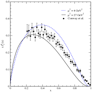
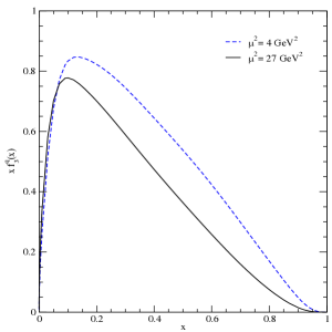
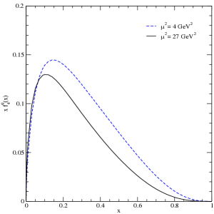
Figure 4: LFQM predictions for the valence PDFs of the pion for a single quark evolved to the scales of $\mu^{2}=(4,27)$ GeV² from from the initial scale $\mu^{2}_{0}=1$ GeV². The experimental data are taken from Ref. Conway .

IV.2 QCD evolution of PDF

The valence quark distributions at higher scales of $\mu^{2}$ can be established using the initial input by undergoing QCD evolution. We utilize the NNLO DGLAP equations Dok ; Gribov ; Altarelli within the framework of QCD to evolve our PDFs from their original model scales to the higher $\mu^{2}$ scales required for experimental comparisons. The scale evolution enables quarks to emit and absorb gluons, with the emitted gluons leading to the generation of quark-antiquark pairs and additional gluons. This process at higher scales unveils the gluon and sea quark constituents within the constituent quarks, revealing their QCD characteristics.

For the QCD evolutions of PDFs, we use the Higher Order Perturbative Parton Evolution toolkit(HOPPET) to numerically solve the NNLO DGLAP equation Rojo and the strong coupling constant $\alpha_{s}(\mu_{0})$ at the initial scale is fixed following the procedure BPT04 ; PS14 ; BAG08 ; CN09 , i.e. the initial scale $\mu_{0}$ needs to be chosen in such a way that, after evolving from $\mu_{0}$ to $\mu=2$ GeV, the valence quarks at $\mu^{2}=4$ GeV² carry about $47\%$ of the total momentum in the pion SMRS ; Capitani . Applying this constraint to the twist-2 PDF, we obtain at $\mu^{2}=4$ GeV²

$$\langle x\rangle_{val}\equiv 2\langle x\rangle^{q}_{1}=2\int^{1}_{0}dx\;xf^{q}_{1}(x)=0.472,$$ (47)

with the following parameter sets in HOPPET

$$\mu_{0,{\rm NNLO}}=1\;{\rm GeV},\;\frac{\alpha_{\rm NNLO}(\mu^{2}_{0})}{2\pi}=0.302.$$ (48)

We subsequently apply QCD evolutions not only to the twist-2 PDF but also to the twist-3 and twist-4 PDFs. We summarize in Tables 3-6 the first few Mellin moments of the pion PDFs, evaluated at both scales $\mu^{2}=(4,27)$ GeV², and compared with other theoretical predictions.

Figure 4 shows the NNLO DGLAP evolutions of $xf^{q}_{i}(x)(i=1,3,4)$ from the initial scale $\mu^{2}_{0}=1$ GeV² evolved to $\mu^{2}=4$ GeV² and $\mu^{2}=27$ GeV². The experimental data are taken from Ref. Conway .

Table 3: Mellin moments of the pion valence PDF, $f^{q}_{1}(x)$, evaluated at the scale $\mu^{2}=4$ GeV².

	$\langle x\rangle^{u}_{t2}$	$\langle x^{2}\rangle^{u}_{t2}$	$\langle x^{3}\rangle^{u}_{t2}$	$\langle x^{4}\rangle^{u}_{t2}$
This work	0.236	0.101	0.055	0.033
Joo	0.2541(26)	0.094(12)	0.057(4)	0.015(12)
Oehm	0.2075(106)	0.163(33)	$-$	$-$
DSE2	0.24(2)	0.098(10)	0.049(7)	$-$
DSE3	0.24(2)	0.094(13)	0.047(8)	$-$

Table 4: Mellin moments of the pion valence PDF, $f^{q}_{1}(x)$, evaluated at the scale $\mu^{2}=27$ GeV².

	$\langle x\rangle^{u}_{t2}$	$\langle x^{2}\rangle^{u}_{t2}$	$\langle x^{3}\rangle^{u}_{t2}$	$\langle x^{4}\rangle^{u}_{t2}$
This work	0.182	0.069	0.034	0.019
Sufian	0.18(3)	0.064(10)	0.030(5)	$-$
DSE3	0.20(2)	0.074(10)	0.035(6)	$-$
Nam12	0.184	0.068	0.033	0.018
WRH	0.217(11)	0.087(5)	0.045(3)	$-$

Table 5: Mellin moments of the twist-3 pion PDF, $f^{q}_{3}(x)$, evaluated at the scales $\mu^{2}=4$ GeV² and $\mu^{2}=27$ GeV², respectively.

	$\langle x\rangle^{u}_{t3}$	$\langle x^{2}\rangle^{u}_{t3}$	$\langle x^{3}\rangle^{u}_{t3}$	$\langle x^{4}\rangle^{u}_{t3}$
$\mu^{2}=4$ GeV2	0.471	0.164	0.079	0.045
$\mu^{2}=27$ GeV2	0.365	0.111	0.049	0.026

Table 6: Mellin moments of the twist-4 pion PDF, $f^{q}_{4}(x)$, evaluated at the scales $\mu^{2}=4$ GeV² and $\mu^{2}=27$ GeV², respectively.

	$\langle x\rangle^{u}_{t4}$	$\langle x^{2}\rangle^{u}_{t4}$	$\langle x^{3}\rangle^{u}_{t4}$	$\langle x^{4}\rangle^{u}_{t4}$
$\mu^{2}=4$ GeV2	0.069	0.021	0.009	0.005
$\mu^{2}=27$ GeV2	0.053	0.014	0.006	0.003

V Summary

We have conducted an investigation of the inter-related pion’s form factor, TMDs, and PDFs within the framework of the LFQM. Our self-consistent LFQM adheres to the BT construction, where the interaction $V_{q{\bar{q}}}$ between the quark and antiquark is integrated into the mass operator through $M:=M_{0}+V_{q{\bar{q}}}$ and the meson state is constructed in terms of constituent quark and antiquark representations maintaining the four-momentum conservation with $M\to M_{0}$ at the meson-quark vertex.

The distinguished feature of our self-consistent LFQM for the analysis lies in the computation of hadronic matrix elements. For the gauge invariant pion form factor, defined by the local matrix element $\langle P^{\prime}|J^{\mu}|P\rangle={\cal P}^{\mu}F_{\pi}(Q^{2})$, where ${\cal P}^{\mu}=(P+P^{\prime})^{\mu}-q^{\mu}(M^{2}-M^{\prime 2})/q^{2}$, we obtain the current component independent pion form factor by taking $M^{(\prime)}\to M^{(\prime)}_{0}$ consistently both in the matrix element and the Lorentz factor ${\cal P}^{\mu}$ and computing $F_{\pi}(Q^{2})=\bra{P^{\prime}}\frac{J^{\mu}}{{\cal P}^{\mu}}\ket{P}$.

Subsequently, we obtain the three unpolarized TMDs and PDFs related with the forward matrix element $\langle P|{\bar{q}}\gamma^{\mu}q|P\rangle$, where the twist-2, 3, and 4 TMDs are obtained from $\mu=+,\perp$, and $-$, respectively. Especially, we resolve the LF zero mode issue of the twist-4 TMD and PDF raised by the authors in Lorce ; LPS16 and show that the twist-4 PDF $f^{q}_{4}(x)$ satisfies the sum rule, $2\int dxf^{q}_{4}(x)=1$, within our LFQM.

In conclusion, our self-consistent LFQM has been successfully applied to various amplitudes, including two-point functions such as decay constants and DAs CJ14 ; CJ15 ; CJ17 ; Jafar1 ; Jafar2 , three-point functions such as semileptonic and rare decays between two pseudoscalar mesons Choi21 ; ChoiAdv , and four-point functions such as TMDs and PDFs as presented in this work. Through these studies, we have demonstrated that our LFQM is capable to accurately account for the LF zero modes that arise when dealing with the challenging $J^{-}$ current. It is noteworthy that the presence of LF zero modes resulting from the $J^{-}$ current appears a common feature to be investigated in LFD. Our innovative approach, particularly in handling the $J^{-}$ current, offers a novel means of correctly extracting and incorporating the zero modes effectively within the LFQM framework. Therefore, extending our approach to encompass additional three-point and four-point functions and related observables warrants thorough investigation to further explore the effects of LF zero modes.

Appendix A Helicity contributions to the pion form factor

Table 7: Dirac matrix elements for the helicity spinors BL80 . Note that $p^{L(R)}q^{R(L)}={\bf p}_{\perp}\cdot{\bf q}_{\perp}\pm i{\bf p}_{\perp}\times{\bf q}_{\perp}$.

Matrix	Helicity ($\lambda\to\lambda^{\prime}$)
elements	$\uparrow\to\uparrow$	$\uparrow\to\downarrow$
${\bar{u}}_{\lambda^{\prime}}\gamma^{\mu}u_{\lambda}$	$\downarrow\to\downarrow$	$\downarrow\to\uparrow$
$\frac{{\bar{u}}_{\lambda^{\prime}}(p_{2})}{\sqrt{p^{+}_{2}}}\gamma^{+}\frac{u_{\lambda}(p_{1})}{\sqrt{p^{+}_{1}}}$	2	0
$\frac{{\bar{u}}_{\lambda^{\prime}}(p_{2})}{\sqrt{p^{+}_{2}}}\gamma^{-}\frac{u_{\lambda}(p_{1})}{\sqrt{p^{+}_{1}}}$	$\frac{2}{p^{+}_{1}p^{+}_{2}}({\bf p}_{2\perp}\cdot{\bf p}_{1\perp}\pm i{\bf p}_{2\perp}\times{\bf p}_{1\perp}+m^{2})$	$\mp\frac{2m}{p^{+}_{1}p^{+}_{2}}[(p^{x}_{2}\pm ip^{y}_{2})-(p^{x}_{1}\pm ip^{y}_{1})]$
$\frac{{\bar{u}}_{\lambda^{\prime}}(p_{2})}{\sqrt{p^{+}_{2}}}\gamma^{i}_{\perp}\frac{u_{\lambda}(p_{1})}{\sqrt{p^{+}_{1}}}$	$\frac{{\bf p}^{i}_{2\perp}\mp i\epsilon^{ij}{\bf p}^{j}_{2\perp}}{p^{+}_{2}}+\frac{{\bf p}^{i}_{1\perp}\pm i\epsilon^{ij}{\bf p}^{j}_{1\perp}}{p^{+}_{1}}$	$\mp m\left(\frac{p^{+}_{2}-p^{+}_{1}}{p^{+}_{1}p^{+}_{2}}\right)(\delta^{i1}\pm i\delta^{i2})$

In this appendix, we provide a summary of the results regarding the helicity contributions to the pion form factor, as presented in Tables 1 and 2. For the analysis of the helicity contributions to the pion form factor, the term corresponding to the spin trace in Eq. (22) can be rewritten as

$$h^{\mu}_{\lambda_{1}{\bar{\lambda}}\to\lambda_{2}{\bar{\lambda}}} \equiv \mathcal{R}^{\dagger}_{\lambda_{2}{\bar{\lambda}}}\left[\frac{\bar{u}_{\lambda_{2}}(p_{2})}{\sqrt{p^{+}_{2}}}\gamma^{\mu}\frac{u_{\lambda_{1}}(p_{1})}{\sqrt{p^{+}_{1}}}\right]\mathcal{R}_{\lambda_{1}{\bar{\lambda}}},$$ (49)

$$= \mathcal{R}^{\dagger}_{\lambda_{2}{\bar{\lambda}}}U^{\mu}_{\lambda_{1}\to\lambda_{2}}\mathcal{R}_{\lambda_{1}{\bar{\lambda}}}$$

where $p^{+}_{i}=x_{i}P^{+}=xP^{+}(i=1,2)$ and the relevant Dirac matrix elements for the helicity spinors BL80 are summarized in Table 7.

Then, we obtain the helicity non-flip and flip contributions, i.e. $h^{\mu}_{(\uparrow\to\uparrow)+(\downarrow\to\downarrow)}\equiv\sum_{{\bar{\lambda}}}(h^{\mu}_{\uparrow{\bar{\lambda}}\to\uparrow{\bar{\lambda}}}+h^{\mu}_{\downarrow{\bar{\lambda}}\to\downarrow{\bar{\lambda}}})$ and $h^{\mu}_{(\uparrow\to\downarrow)+(\downarrow\to\uparrow)}\equiv\sum_{{\bar{\lambda}}}(h^{\mu}_{\uparrow{\bar{\lambda}}\to\downarrow{\bar{\lambda}}}+h^{\mu}_{\downarrow{\bar{\lambda}}\to\uparrow{\bar{\lambda}}})$, respectively, for each component ($\mu=+,\perp,-)$ of the current as follows:

(1) For the ${\cal J}^{+}_{\rm em}$ current: The helicity flip contributions are zero, i.e. $h^{+}_{(\uparrow\to\downarrow)+(\downarrow\to\uparrow)}=0$, and only the helicity non-flip elements contribute. Specifically, we obtain

$$h^{+}_{(\uparrow\to\uparrow)+(\downarrow\to\downarrow)}$$

$$=2(\mathcal{R}^{\dagger}_{\uparrow\uparrow}\mathcal{R}_{\uparrow\uparrow}+\mathcal{R}^{\dagger}_{\uparrow\downarrow}\mathcal{R}_{\uparrow\downarrow}+\mathcal{R}^{\dagger}_{\downarrow\uparrow}\mathcal{R}_{\downarrow\uparrow}+\mathcal{R}^{\dagger}_{\downarrow\downarrow}\mathcal{R}_{\downarrow\downarrow})$$

$$=\frac{2(m^{2}+{\bf k}_{\perp}\cdot{\bf k}^{\prime}_{\perp})}{\sqrt{m^{2}+{\bf k}^{2}_{\perp}}\sqrt{m^{2}+{\bf k}^{\prime 2}_{\perp}}}.$$ (50)

(2) For the ${\bf{\cal J}}^{\perp}_{\rm em}$ current: As in the case of the plus current, only the helicity non-flip elements contribute. For convenience, we compute the matrix elements for $\gamma_{\perp}\cdot{\bf q}_{\perp}$ rather than those for $\gamma_{\perp}$, i.e.,

$$U^{\perp}_{\uparrow\to\uparrow}\cdot{\bf q}_{\perp}=\left[U^{\perp}_{\downarrow\to\downarrow}\cdot{\bf q}_{\perp}\right]^{*}=\frac{p^{R}_{1}q^{L}}{p^{+}_{1}}+\frac{p^{L}_{2}q^{R}}{p^{+}_{2}},$$ (51)

where $p^{R}=p_{x}+ip_{y}$ and $p^{L}=p_{x}-ip_{y}$. We then obtain

$$(h^{\perp}\cdot{\bf q}_{\perp})_{(\uparrow\to\uparrow)+(\downarrow\to\downarrow)}$$ (52)

$$=(U^{\perp}_{\uparrow\to\uparrow}\cdot{\bf q}_{\perp})(\mathcal{R}^{\dagger}_{\uparrow\uparrow}\mathcal{R}_{\uparrow\uparrow}+\mathcal{R}^{\dagger}_{\uparrow\downarrow}\mathcal{R}_{\uparrow\downarrow})$$

$$\hskip 8.5359pt+(U^{\perp}_{\downarrow\to\downarrow}\cdot{\bf q}_{\perp})(\mathcal{R}^{\dagger}_{\downarrow\uparrow}\mathcal{R}_{\downarrow\uparrow}+\mathcal{R}^{\dagger}_{\downarrow\downarrow}\mathcal{R}_{\downarrow\downarrow})$$

$$=\frac{-(m^{2}+{\bf k}_{\perp}\cdot{\bf k}^{\prime}_{\perp})({\bf q}^{2}_{\perp}+2{\bf k}_{\perp}\cdot{\bf q}_{\perp})}{xP^{+}\sqrt{m^{2}+{\bf k}^{2}_{\perp}}\sqrt{m^{2}+{\bf k}^{\prime 2}_{\perp}}}.$$

(3) For the ${\cal J}^{-}_{\rm em}$ current: In this case, not only the helicity non-flip but also the helicity flip elements contribute. Specifically, we obtain

$$\sum_{{\bar{\lambda}}}h^{-}_{\uparrow{\bar{\lambda}}\to\uparrow{\bar{\lambda}}} = U^{-}_{\uparrow\to\uparrow}(\mathcal{R}^{\dagger}_{\uparrow\uparrow}\mathcal{R}_{\uparrow\uparrow}+\mathcal{R}^{\dagger}_{\uparrow\downarrow}\mathcal{R}_{\uparrow\downarrow})$$ (53)

$$= \frac{(p^{L}_{2}p^{R}_{1}+m^{2})(k^{\prime R}k^{L}+m^{2})}{p^{+}_{1}p^{+}_{2}\sqrt{m^{2}+{\bf k}^{2}_{\perp}}\sqrt{m^{2}+{\bf k}^{\prime 2}_{\perp}}},$$

$$\sum_{{\bar{\lambda}}}h^{-}_{\downarrow{\bar{\lambda}}\to\downarrow{\bar{\lambda}}} = U^{-}_{\downarrow\to\downarrow}(\mathcal{R}^{\dagger}_{\downarrow\uparrow}\mathcal{R}_{\downarrow\uparrow}+\mathcal{R}^{\dagger}_{\downarrow\downarrow}\mathcal{R}_{\downarrow\downarrow})$$ (54)

$$= \frac{(p^{R}_{2}p^{L}_{1}+m^{2})(k^{\prime L}k^{R}+m^{2})}{p^{+}_{1}p^{+}_{2}\sqrt{m^{2}+{\bf k}^{2}_{\perp}}\sqrt{m^{2}+{\bf k}^{\prime 2}_{\perp}}},$$

$$\sum_{{\bar{\lambda}}}h^{-}_{\uparrow{\bar{\lambda}}\to\downarrow{\bar{\lambda}}} = U^{-}_{\uparrow\to\downarrow}(\mathcal{R}^{\dagger}_{\downarrow\uparrow}\mathcal{R}_{\uparrow\uparrow}+\mathcal{R}^{\dagger}_{\downarrow\downarrow}\mathcal{R}_{\uparrow\downarrow})$$ (55)

$$= \frac{m^{2}(p_{2}-p_{1})^{R}(k-k^{\prime})^{L}}{p^{+}_{1}p^{+}_{2}\sqrt{m^{2}+{\bf k}^{2}_{\perp}}\sqrt{m^{2}+{\bf k}^{\prime 2}_{\perp}}},$$

$$\sum_{{\bar{\lambda}}}h^{-}_{\downarrow{\bar{\lambda}}\to\uparrow{\bar{\lambda}}} = U^{-}_{\downarrow\to\uparrow}(\mathcal{R}^{\dagger}_{\uparrow\uparrow}\mathcal{R}_{\downarrow\uparrow}+\mathcal{R}^{\dagger}_{\uparrow\downarrow}\mathcal{R}_{\downarrow\downarrow})$$ (56)

$$= \frac{m^{2}(p_{2}-p_{1})^{L}(k-k^{\prime})^{R}}{p^{+}_{1}p^{+}_{2}\sqrt{m^{2}+{\bf k}^{2}_{\perp}}\sqrt{m^{2}+{\bf k}^{\prime 2}_{\perp}}}.$$

We note that $p_{1}^{L(R)}-p_{2}^{L(R)}=q^{L(R)}$ and $k^{\prime L(R)}-k^{L(R)}=(1-x)q^{L(R)}$ since ${\bf p}_{1\perp}-{\bf p}_{2\perp}={\bf q}_{\perp}$ and ${\bf k}^{\prime}_{\perp}-{\bf k}_{\perp}=(1-x){\bf q}_{\perp}$ as given in Eq. (III). Thus, we get the helicity flip contributions from Eqs. (A7) and (A8) as follows

$$h^{-}_{(\uparrow\to\downarrow)+(\downarrow\to\uparrow)}=\frac{2m^{2}(1-x){\bf q}^{2}_{\perp}}{p^{+}_{1}p^{+}_{2}\sqrt{m^{2}+{\bf k}^{2}_{\perp}}\sqrt{m^{2}+{\bf k}^{\prime 2}_{\perp}}}.$$ (57)

The helicity non-flip contributions can be obtained using Eqs. (A5) and (A6) together with the relations ${\bf p}_{1\perp}\times{\bf p}_{2\perp}={\bf k}_{\perp}\times{\bf q}_{\perp}$ and ${\bf p}_{1\perp}\cdot{\bf p}_{2\perp}={\bf k}^{2}_{\perp}+{\bf k}_{\perp}\cdot{\bf q}_{\perp}$. This yields the following expressions:

$$h^{-}_{(\uparrow\to\uparrow)+(\downarrow\to\downarrow)}$$

$$=\frac{2}{p^{+}_{1}p^{+}_{2}{\cal K}}\biggl{\{}({\bf k}_{\perp}\cdot{\bf k}^{\prime}_{\perp}+m^{2})({\bf k}^{2}_{\perp}+{\bf k}_{\perp}\cdot{\bf q}_{\perp}+m^{2})$$

$$\hskip 51.21504pt+\;(1-x)({\bf k}_{\perp}\times{\bf q}_{\perp})^{2}\biggr{\}},$$ (58)

where ${\cal K}=\sqrt{m^{2}+{\bf k}^{2}_{\perp}}\sqrt{m^{2}+{\bf k}^{\prime 2}_{\perp}}$.

Appendix B Link between the covariant BS model and the LFQM

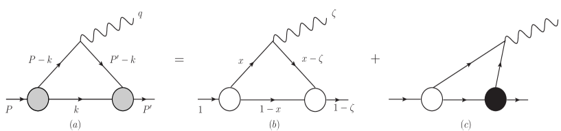
Figure 5: The covariant triangle diagram (a) corresponds to the sum of the LF valence diagram (b) and the nonvalence diagram (c), where $\zeta=q^{+}/P^{+}$. The large white and black blobs at the meson-quark vertices in (b) and (c) represent the ordinary LF wave function and the nonvalence wave function vertices, respectively.

In this appendix, we show the derivation of pion form factor in the LFQM starting from the covariant BS model using the matching condition known as the “type II” link CJ14 between the two models.

The Feynman covariant triangle diagram shown in Fig. 5(a) describes the transition of a pseudoscalar meson with momentum $P$ and mass $M$ to another pseudoscalar meson with momentum $P^{\prime}$ and mass $M^{\prime}$, where $q=P-P^{\prime}$ is the four-momentum transfer. The matrix element ${\cal J}^{\mu}\equiv\langle P^{\prime}|\bar{q}\gamma^{\mu}q|P\rangle$ obtained from the covariant BS model of Fig. 5(a) is given by

$${\cal J}^{\mu}=iN_{c}\int\frac{d^{4}k}{(2\pi)^{4}}\frac{H^{\prime}_{0}H^{\prime\prime}_{0}}{N_{p_{1}}N_{k}N_{p_{2}}}S^{\mu},$$ (59)

where

$$S^{\mu}={\rm Tr}[\gamma_{5}(\not{p}_{2}+m_{q})\gamma^{\mu}(\not{p}_{1}+m_{q})\gamma_{5}(-\not{k}+m_{\bar{q}})],$$ (60)

and $p_{1}=P-k$ and $p_{2}=P^{\prime}-k$ are the momenta of the active quark with mass $m_{q}$ and $k$ is the momentum of the spectator quark with mass $m_{\bar{q}}$. The denominator factors $N_{p_{1(2)},k}$ are given by $N_{p_{1(2)}}=p^{2}_{1(2)}-m^{2}_{q}+i\epsilon$ and $N_{k}=k^{2}-m^{2}_{\bar{q}}+i\epsilon$. We take the vertex functions as $H^{\prime}_{0}=H^{\prime}_{0}(p^{2}_{1},k^{2})=g/(N^{\prime}_{\Lambda})^{n}$ and $H^{\prime\prime}_{0}=H^{\prime\prime}_{0}(p^{2}_{2},k^{2})=g/(N^{\prime\prime}_{\Lambda})^{n}$ with $N^{\prime}_{\Lambda}(N^{\prime\prime}_{\Lambda})=p^{2}_{1}(p^{2}_{2})-\Lambda^{2}+i\epsilon$.

Following the same procedure using the Feynman parametrization CJ09 , we obtain the manifestly covariant result of $F_{\rm em}(q^{2})\equiv F_{\pi}(q^{2})$ for $n=1$ case as

$$F^{\rm cov}_{\pi}(q^{2}) = {\cal N}\int^{1}_{0}dx\int^{1-x}_{0}dy\biggl{\{}[3(x+y)-4]\ln C_{1}$$ (61)

$$+\biggl{[}(1-x-y)^{2}(x+y)M^{2}$$

$$+(2-x-y)(m^{2}+xyq^{2})\biggr{]}C_{2}\biggr{\}},$$

where ${\cal N}=g^{2}N_{c}/8\pi^{2}(\Lambda^{2}-m^{2})^{2}$, $C_{1}=\frac{C_{\Lambda m}C_{m\Lambda}}{C_{\Lambda\Lambda}C_{mm}}$, and $C_{2}=(1/C_{\Lambda\Lambda}-1/C_{\Lambda m}-1/C_{m\Lambda}+1/C_{mm})$ with $C_{\alpha\beta}=(1-x-y)(x+y)M^{2}+xyq^{2}-(x\alpha^{2}+y\beta^{2})-(1-x-y)m^{2}$. Note that the logarithmic term, $\ln C_{1}$, is obtained from the dimensional regularization with the Wick rotation.

Essentially, the Feynman covariant triangle diagram in Fig. 5(a) is equivalent to the sum of the LF valence diagram in Fig. 5(b) and the nonvalence diagram in Fig. 5(c), where $\zeta=q^{+}/P^{+}$. In the valence region ($0<k^{+}<P^{\prime+}$), the pole $k^{-}=k^{-}_{\rm on}=({\bf k}^{2}_{\perp}+m^{2}-i\epsilon)/k^{+}$ (i.e., the spectator quark) is located in the lower half of the complex $k^{-}$ plane. In the nonvalence region ($P^{\prime+}<k^{+}<P^{+}$), the poles are at $p^{-}_{1}=p^{-}_{1\rm on}(m_{1})=[m^{2}+{\bf k}^{2}_{\perp}-i\epsilon]/p^{+}_{1}$ (from the struck quark propagator) and $p^{-}_{1}=p^{-}_{1\rm on}(\Lambda)=[\Lambda^{2}+{\bf k}^{2}_{\perp}-i\epsilon]/p^{+}_{1}$ (from the vertex function $H^{\prime}_{0}$), which are located in the upper half of the complex $k^{-}$ plane.

Performing the LF calculation of Eq. (18) together with Eq. (III), one obtains $F^{(\mu)}_{\pi}$ for all possible three different components ($\mu=\pm,\perp$) of the current as follows:

$$F^{(+)}_{\pi}=\frac{{\cal J}^{+}_{\rm em}}{2P^{+}},$$

$$F^{(\perp)}_{\pi}=\frac{{\cal J}^{\perp}_{\rm em}\cdot{\bf q}_{\perp}}{\Delta M^{2}-{\bf q}^{2}_{\perp}},$$

$$F^{(-)}_{\pi}=\frac{{\bf q}^{2}_{\perp}P^{+}{\cal J}^{-}_{\rm em}}{2M^{\prime 2}{\bf q}^{2}_{\perp}+{\bf q}^{4}_{\perp}+(\Delta M^{2})^{2}},$$ (62)

where $\Delta M^{2}=M^{2}-M^{\prime 2}$. If the nonvalence diagram ($P^{\prime+}<k^{+}<P^{+}$) does not vanish as $q^{+}\to 0$, this nonvanishing contribution is called the LF zero mode. In the LF calculation of the covariant BS model, we do not quantify the possible zero modes for the calculations of $F^{(\pm,\perp)}_{\pi}$ given by Eq. (B). Instead, we just determine the existence/nonexistence of the zero mode contribution to $F^{(\pm,\perp)}_{\pi}$ by computing only the valence contribution in the $q^{+}=0$ frame. We then compare the covariant BS model to the standard LFQM and discuss the implication of the LF zero mode between the two models.

The LF calculation for the trace term in Eq. (60) can be separated into the on-shell propagating part $S^{\mu}_{\rm on}$ and the instantaneous part $S^{\mu}_{\rm inst}$, i.e. $S^{\mu}=S^{\mu}_{\rm on}+S^{\mu}_{\rm inst}$, via the relation between the Feynman propagator ($\not{p}+m$) and the LF on-mass shell propagator ($\not{p}_{\rm on}+m$)

$$(\not{p}+m)=(\not{p}_{\rm on}+m)+\gamma^{+}\frac{(p^{-}-p^{-}_{\rm on})}{2}.$$ (63)

The trace term $S^{\mu}_{\rm on}$ obtained from the on-shell propagating part is given by

$$S^{\mu}_{\rm on} = 4[p^{\mu}_{1\rm on}(p_{2\rm on}\cdot k_{\rm on}+m^{2})-k^{\mu}_{\rm on}(p_{1\rm on}\cdot p_{2\rm on}-m^{2})$$ (64)

$$+p^{\mu}_{2\rm on}(p_{1\rm on}\cdot k_{\rm on}+m^{2})],$$

where

$$p_{1\rm on} = \left(xP^{+},\frac{m^{2}+{\bf k}_{\perp}^{2}}{xP^{+}},-{\bf k}_{\perp}\right),$$

$$p_{2\rm on} = \left(xP^{+},\frac{m^{2}+({\bf k}_{\perp}+{\bf q}_{\perp})^{2}}{xP^{+}},-{\bf k}_{\perp}-{\bf q}_{\perp}\right),$$

$$k_{\rm on} = \left((1-x)P^{+},\frac{m^{2}+{\bf k}_{\perp}^{2}}{(1-x)P^{+}},{\bf k}_{\perp}\right).$$ (65)

The instantaneous contribution is obtained as

$$S^{\mu}_{\rm inst} = 2\Delta_{p_{1}}\left[g^{+\mu}(k\cdot p_{2}+m^{2})+p^{\mu}_{2}k^{+}-p^{+}_{2}k^{\mu}\right],$$ (66)

$$+2\Delta_{p_{2}}\left[g^{+\mu}(k\cdot p_{1}+m^{2})+p^{\mu}_{1}k^{+}-p^{+}_{1}k^{\mu}\right],$$

$$+2\Delta_{k}\left[g^{+\mu}(-p_{1}\cdot p_{2}+m^{2})+p^{\mu}_{1}p^{+}_{2}+p^{+}_{1}p^{\mu}_{2}\right],$$

$$+2\Delta_{p_{1}}\Delta_{p_{2}}k^{+}g^{+\mu},$$

where $\Delta_{p}=(p^{-}-p^{-}_{\rm on})$. We note for the valence contribution (i.e. $k^{-}=k^{-}_{\rm on}$) that $\Delta_{p_{1(2)}}=(M^{2}-M^{(\prime)2}_{0})/P^{+}$, where

$$M^{(\prime)2}_{0}=\frac{{\bf k}^{(\prime)2}_{\perp}+m^{2}}{x}+\frac{{\bf k}^{(\prime)2}_{\perp}+m^{2}}{1-x}$$ (67)

is the invariant mass of the initial (final) state meson and ${\bf k}^{\prime}_{\perp}={\bf k}_{\perp}+(1-x){\bf q}_{\perp}$. One can see from Eq. (66) that there is no instantaneous contribution for the plus current, i.e. $S^{+}_{\rm inst}=0$.

Now, for the valence region $(0<x<1)$ in the $q^{+}=0$ frame, the LF amplitude obtained from the on-shell contribution is given by

$${\cal J}^{\mu}_{\rm em}=\frac{N_{c}}{16\pi^{3}}\int^{1}_{0}\frac{dx}{(1-x)}\int d^{2}{\bf k}_{\perp}\chi(x,{\bf k}_{\perp})\chi^{\prime}(x,{\bf k}^{\prime}_{\perp})S^{\mu}_{\rm on},$$ (68)

where

$$\chi(x,{\bf k}_{\perp})=\frac{g}{[x(M^{2}-M^{2}_{0})][x(M^{2}-M^{2}_{\Lambda})]},$$ (69)

for the vertex function with $n=1$ case and $M^{2}_{\Lambda}=M^{2}_{0}(m_{q}\to\Lambda)$. The final state vertex function $\chi^{\prime}$ is obtained from $\chi$ replacing ${\bf k}_{\perp}$ with ${\bf k}^{\prime}_{\perp}$. The trace terms $S^{\mu}_{\rm on}$ for each component of the current are given by

$$S^{+}_{\rm on} = \frac{4P^{+}}{1-x}({\bf k}_{\perp}\cdot{\bf k}^{\prime}_{\perp}+m^{2}),$$

$$S^{\perp}_{\rm on} = -\frac{2(2{\bf k}_{\perp}+{\bf q}_{\perp})}{x(1-x)}({\bf k}_{\perp}\cdot{\bf k}^{\prime}_{\perp}+m^{2}),$$

$$S^{-}_{\rm on} = \frac{4M^{2}_{0}}{xP^{+}}({\bf k}_{\perp}\cdot{\bf k}^{\prime}_{\perp}+m^{2}+{\bf q}_{\perp}\cdot{\bf k}^{\prime}_{\perp}).$$ (70)

Table 8: The operators ${\cal O}^{(\mu)}_{\rm BS}$ defined in Eq. (71), where $\Delta M^{2}=0$ in the BS model but $\Delta M^{2}=M^{2}_{0}-M^{\prime 2}_{0}$ in the standard LFQM.

$F^{(\mu)}_{\pi}$	${\cal O}^{(\mu)}_{\rm BS}$	${\cal O}^{(\mu)}_{\rm LFQM}$
$F^{(+)}_{\pi}$	${\bf k}_{\perp}\cdot{\bf k}^{\prime}_{\perp}+m^{2}$	${\cal O}^{(+)}_{\rm BS}$
$F^{(\perp)}_{\pi}$	$\frac{({\bf k}_{\perp}\cdot{\bf k}^{\prime}_{\perp}+m^{2})({\bf q}^{2}_{\perp}+2{\bf k}_{\perp}\cdot{\bf q}_{\perp})}{x({\bf q}^{2}_{\perp}-\Delta M^{2})}$	${\cal O}^{(\perp)}_{\rm BS}(M^{(\prime)}\to M^{(\prime)}_{0})$
$F^{(-)}_{\pi}$	$\frac{2(1-x){\bf q}^{2}_{\perp}M^{2}_{0}({\bf k}_{\perp}\cdot{\bf k}^{\prime}_{\perp}+m^{2}+{\bf q}_{\perp}\cdot{\bf k}^{\prime}_{\perp})}{x[2M^{\prime 2}{\bf q}^{2}_{\perp}+{\bf q}^{4}_{\perp}+(\Delta M^{2})^{2}]}$	${\cal O}^{(-)}_{\rm BS}(M^{(\prime)}\to M^{(\prime)}_{0})$

From Eqs. (B) and (68), we get the on-shell contributions to the pion form factor for each current component $(\mu=\pm,\perp)$ as follows

$$F^{(\mu)}_{\pi}(Q^{2})=N_{c}\int^{1}_{0}dx\int\frac{d^{2}{\bf k}_{\perp}}{8\pi^{3}}\frac{\chi(x,{\bf k}_{\perp})\chi^{\prime}(x,{\bf k}^{\prime}_{\perp})}{(1-x)^{2}}{\cal O}^{(\mu)}_{\rm BS},$$ (71)

where the operators ${\cal O}^{(\mu)}_{\rm BS}(x,{\bf k}_{\perp})$ corresponding to the three different components $(\mu=\pm,\perp)$ of the current are summarized in Table 8, where $\Delta M^{2}=0$ in this BS model. In this BS model, we found numerically that the LF on-shell results obtained from the plus and perpendicular components of the current in Eq. (71) are exactly the same as the covariant one in Eq. (61), $F^{\rm cov}_{\pi}=F_{\pi}^{(+)}=F_{\pi}^{(\perp)}$. This indicates that the LF results $F_{\pi}^{(+)}=F_{\pi}^{(\perp)}$ receive only the on-shell contributions in the valence region. Especially, the two results, $F_{\pi}^{(+)}$ and $F_{\pi}^{(\perp)}$, are analytically the same, which can be easily checked by using the symmetric variable , i.e. ${\bf k}_{\perp}={\bf l}_{\perp}-\frac{(1-x)}{2}{\bf q}_{\perp}$ and ${\bf k}^{\prime}_{\perp}={\bf l}_{\perp}+\frac{(1-x)}{2}{\bf q}_{\perp}$. We note from using ${\bf l}_{\perp}$ that $\chi(x,{\bf k}_{\perp})\chi^{\prime}(x,{\bf k}^{\prime}_{\perp})$ can be expressed as only even powers of ${\bf l}_{\perp}$ and $\cos\theta$ where $\cos\theta$ is defined through ${\bf l}_{\perp}\cdot{\bf q}_{\perp}=|{\bf l}_{\perp}||{\bf q}_{\perp}|\cos\theta$.

While it is well-known that the plus component of the current receives only the on-shell contribution, the present result ($F^{\rm cov}_{\pi}=F_{\pi}^{(\perp)}$) obtained from the perpendicular current with only the on-shell contribution may be regarded coincidental since this component in general receives the non-vanishing instantaneous contribution even in the valence region and possibly LF zero mode. The similar observation for the perpendicular current has been made in MS02 , where $\mu=y$ was chosen in the $q^{+}=0$ with ${\bf q}_{\perp}=(q_{x},0)$ frame. On the other hand, it is well understood that the LF result $F_{\pi}^{(-)}$ obtained from the on-shell contribution doesn’t match with the covariant result as the minus current requires not only the instantaneous in the valence region but also the zero mode contribution to yield the covariant result.

However, the current component independent pion form factor in our LFQM can be obtained from the BS result, $F^{(\mu)}_{\pi}$ given by Eq. (71), applying the link between the BS model and the LFQM, i.e.,

$$\sqrt{2N_{c}}\frac{\chi^{(\prime)}(x,{\bf k}^{(\prime)}_{\perp})}{(1-x)}\to\frac{\phi^{(\prime)}(x,{\bf k}^{(\prime)}_{\perp})}{\sqrt{m^{2}+{\bf k}^{(\prime)2}_{\perp}}},\;M^{(\prime)}\to M^{(\prime)}_{0},$$ (72)

in Eq. (71), where $\phi(x,{\bf k}_{\perp})$ is the radial wave function in our LFQM. The corresponding operators $\mathcal{O}^{(\mu)}_{\rm LFQM}$ in our LFQM obtained from $\mathcal{O}^{(\mu)}_{\rm BS}$ are also summarized in Table 8. The essential feature of $\mathcal{O}^{(\mu)}_{\rm LFQM}$ compared to $\mathcal{O}^{(\mu)}_{\rm BS}$ lies in the nonvanishing structure of $\Delta M^{2}\to\Delta M^{2}_{0}=M^{2}_{0}-M^{\prime 2}_{0}$ in our LFQM while $\Delta M^{2}=0$ in the covariant BS model for the elastic process.

Applying the link given by Eq.  (72) to Eq. (71), we obtain the same LFQM results for the pion form factor given by Eq. (24), i.e.

$$F^{(\mu)}_{\pi}(Q^{2})=\int^{1}_{0}dx\int\frac{d^{2}{\bf k}_{\perp}}{16\pi^{3}}\frac{\phi(x,{\bf k}_{\perp})\phi^{\prime}(x,{\bf k}^{\prime}_{\perp})}{\sqrt{{\bf k}^{2}_{\perp}+m^{2}}\sqrt{{\bf k}^{\prime 2}_{\perp}+m^{2}}}{\cal O}^{(\mu)}_{\rm LFQM}.$$ (73)

Appendix C Quark mass evolution in the pion form factor

In this appendix, we present our numerical results for the pion form factor and investigate the influence of the quark running mass, treating it exclusively as a function of the momentum transfer $Q^{2}$.

Contrary to quark models or LFQM, which employ a phenomenological constant constituent quark mass, an alternative approach rooted in QCD quantum field theory is the utilization of the BS equation along with the Dyson-Schwinger (DS) equations for the quark propagators, gluon propagator, and vertices. A noteworthy outcome of the DS calculations DS1 ; DS2 is the determination of the effective running mass, $m(p^{2})$ as a function of the Euclidean momentum $p$.

In our earlier study Kiss01 , we examined the impact of the mass evolution from current to constituent quark on the soft contribution to the elastic pion form factor. This was accomplished by employing a light-front BS (LFBS) model, which incorporates a running mass in a LFQM. Specifically, we introduced two algebraic representations of the quark running mass: a crossing asymmetric (CA) mass function, proportional to $p^{2}$, and a crossing symmetric (CS) mass function, proportional to $p^{4}$. In Ref. Kiss01 , we related the four momentum $p^{2}$ to LF variables $(x,{\bf k}_{\perp})$ by utilizing the on-mass shell condition, denoted as $p^{2}=m^{2}(p^{2})$. This condition indicates that the mock meson has no binding energy and results in the following relation: $p^{2}=x(1-x){\tilde{M}}^{2}-{\bf k}^{2}_{\perp}$, where ${\tilde{M}}=(M_{\pi}+3M_{\rho})_{\rm exp}/4=612$ MeV. The Ball-Chiu ansatz was also used to maintain local gauge invariance of the quark-photon vertex.

In this study, we depart from considering the mass evolution dependent on the internal momentum of quark and antiquark. Instead, we aim to evaluate the influence of the quark running mass on the pion form factor by treating mass evolution solely as a function of the momentum transfer $Q^{2}$. This approach is pursued independently of the specific dynamics and internal momentum details. To facilitate this analysis, we introduce two distinct algebraic representations of the quark running mass, i.e., mass functions proportional to $Q^{2}$ and $Q^{4}$ as:

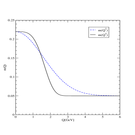
Figure 6: Quark mass evolution $m(Q^{2})$ and $m(Q^{4})$ in spacelike momentum transfer ($Q^{2}>0$) region.

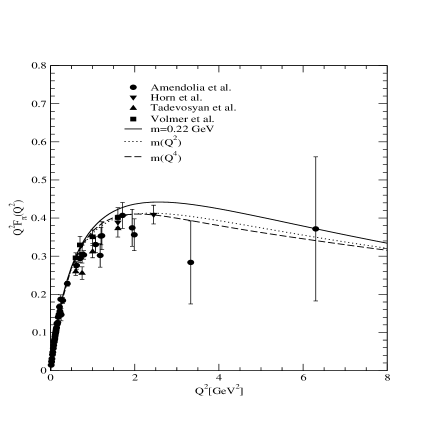
Figure 7: Predictions of $Q^{2}F_{\pi}(Q^{2})$ obtained from the constituent quark mass $m=220$ MeV (solid line), $m(Q^{2})$ (dotted line), and $m^{2}(Q^{4})$ (dashed line), respectively. The experimental data are taken from Amen86 ; Volmer ; Tade ; Horn .

$$m(Q^{2}) = m_{0}+(m-m_{0})\exp(-Q^{2}/\mu^{2}),$$

$$m(Q^{4}) = m_{0}+(m-m_{0})\exp(-Q^{4}/\lambda^{4}),$$ (74)

where $m_{0}$ and $m$ are the current and constituent quark masses, respectively. The parameters $\mu$ and $\lambda$ are used to adjust the shape of the mass evolution so that the running mass yields a generic picture of the quark mass evolution from the low energy limit of the constituent quark mass to the high energy limit of the current quark mass. We use $m_{0}=5$ MeV, $m=220$ MeV, $\mu^{2}=5$ GeV², and $\lambda^{4}=10$ GeV⁴, respectively.

In Fig. 6, we depict the evolution of the quark mass $m(Q^{2})$ and $m(Q^{4})$ in the spacelike momentum transfer region ($Q^{2}>0$). Furthermore, Fig. 7 presents our results for $Q^{2}F_{\pi}(Q^{2})$, showcasing the constituent quark mass $m=220$ MeV (solid line) alongside the running mass functions $m(Q^{2})$ (dotted line) and $m^{2}(Q^{4})$ (dashed line) for the intermediate $Q^{2}$ range. These results are then compared with experimental data Amen86 ; Volmer ; Tade ; Horn .

As discussed in Sec.III, the result obtained from the constituent quark mass given by Eq. (24) is completely independent of the current component $J^{\mu}$. In comparison to the case of constituent quark mass, the form factor with $Q^{2}$-dependent quark mass exhibits a faster fall-off at intermediate $Q^{2}$ range. This behavior resembles the quark mass evolution through internal momenta of quark and antiquark, as discussed in Kiss01 , and appears to provide somewhat better description closer to the experimental data. Further, the symmetric form of quark mass evolution with $m(Q^{4})$ exhibits a slightly faster fall-off compared to the asymmetric form with $m(Q^{2})$. However, the difference in the rate of fall-off between the two forms seems not so significant.

References

- (1) G. P. Lepage and S. J. Brodsky, Exclusive processes in perturbative quantum chromodynamics, Phys. Rev. D 22, 2157 (1980).
- (2) M. V. Polyakov and C. Weiss, Skewed and double distributions in the pion and the nucleon, Phys. Rev. D 60, 114017 (1999).
- (3) C. D. Roberts and A. G. Williams, Dyson-Schwinger equations and their application to hadronic physics, Prog. Part. Nucl. Phys. 33, 477 (1994).
- (4) C. Lorcé, B. Pasquini, and P. Schweitzer, Unpolarized transverse momentum dependent parton distribution functions beyond leading twist in quark models, JHEP 01, 103 (2015).
- (5) C. Lorcé, B. Pasquini, and P. Schweitzer, Transverse pion structure beyond leading twist in constituent models, Eur. Phys. J. C 76, 415 (2016).
- (6) G. F. de Teramond, T. Liu, R. S. Sufian, H. G. Dosch. S. J. Brodsky, and A. Deur (HLFHS Collaboration), Universality of Generalized Parton Distributions in Light-Front Holographic QCD, Phys. Rev. Lett. 120, 182001 (2018).
- (7) P. C. Barry, N. Sato, W. Melnitchouk, and C.-R. Ji, First Monte Carlo Global QCD Analysis of Pion Parton Distributions, Phys. Rev. Lett. 121, 152001 (2018).
- (8) S. R. Amendolia et al., A measurement of the pion charge radius, Phys. Lett. B 146, 116 (1984).
- (9) E. B. Dally et al., Elastic-Scattering Measurement of the Negative-Pion Radius, Phys. Rev. Lett. 48, 375 (1982).
- (10) S. R. Amendolia et al., A measurement of the space-like pion electromagnetic form factor, Nucl. Phys. B 277, 168 (1986).
- (11) J. Volmer et al., Measurement of the Charged Pion Electromagnetic Form Factor, Phys. Rev. Lett. 86, 1713 (2001).
- (12) V. Tadevosyan et al., Determination of the pion charge form factor for = 0.60-1.60 GeV2, Phys. Rev. C 75, 055205 (2007).
- (13) T. Horn et al., Determination of the Pion Charge Form Factor at and 2.45 , Phys. Rev. Lett. 97, 192001 (2006); Scaling study of the pion electroproduction cross sections, Phys. Rev. C 78, 058201 (2008).
- (14) S.D. Drell, T.M. Yan, Massive Lepton-Pair Production in Hadron-Hadron Collisions at High Energies, Phys. Rev. Lett. 25, 316 (1970)[Erratum: Phys. Rev. Lett. 25, 902 (1970)].
- (15) J.F. Owens, -dependent parametrizations of pion parton distribution functions, Phys. Rev. D 30, 943 (1984).
- (16) M. Gluck, E. Reya, and A. Vogt, Pionic parton distributions, Z. Phys. C 53, 651 (1992).
- (17) P. J. Sutton, A. D. Martin, R. G. Roberts, and W. J. Stirling, Parton distributions for the pion extracted from Drell-Yan and prompt photon experiments, Phys. Rev. D 45, 2349 (1992).
- (18) M. Gluck, E. Reya, and I. Schienbein, Pionic parton distributions revisited, Eur. Phys. J. C 10, 313 (1999).
- (19) K. Wijesooriya, P. E. Reimer, and R. J. Holt, Pion parton distribution function in the valence region, Phys. Rev. C 72, 065203 (2005).
- (20) S. Arnold, A. Metz, abd M. Schlegel, Dilepton production from polarized hadron hadron collisions, Phys. Rev. D 79, 034005 (2009).
- (21) W. Jaus, Relativistic constituent-quark model of electroweak properties of light mesons, Phys. Rev. D 44, 2851 (1991).
- (22) W. Jaus, Semileptonic decays of and mesons in the light-front formalism, Phys. Rev. D 41, 3394 (1990).
- (23) H.-Y. Cheng, C.-Y. Cheung, and C.-W. Hwang, Mesonic form factors and the Isgur-Wise function on the light front, Phys. Rev. D 55, 1559 (1997).
- (24) F. Coester and W. N. Polyzou, Charge form factors of quark-model pions, Phys. Rev. C 71, 028202 (2005).
- (25) H.-M. Choi and C.-R. Ji, Mixing angles and electromagnetic properties of ground state pseudoscalar and vector meson nonets in the light-cone quark model, Phys. Rev. D 59, 074015 (1999).
- (26) H.-M. Choi and C.-R. Ji, Light-front quark model analysis of exclusive semileptonic heavy meson decays, Phys. Lett. B 460, 461 (1999).
- (27) H.-M. Choi and C.-R. Ji, Distribution amplitudes and decay constants for mesons in the light-front quark model, Phys. Rev. D 75, 034019 (2007).
- (28) H.-M. Choi, Decay constants and radiative decays of heavy mesons in light-front quark model, Phys. Rev. D 75, 073016 (2007).
- (29) H.-M. Choi, C.-R. Ji, Z. Li, and H.-Y. Ryu, Variational analysis of mass spectra and decay constants for ground state pseudoscalar and vector mesons in the light-front quark model, Phys. Rev. C 92, 055203 (2015).
- (30) A. J. Arifi, H.-M. Choi, C.-R. Ji, and Y. Oh, Mixing effects on and state heavy mesons in the light-front quark model, Phys. Rev. D 106, 014009 (2022).
- (31) S. J. Brodsky, H.-C. Pauli, and S. S. Pinsky, Quantum chromodynamics and other field theories on the light cone, Phys. Rept. 301, 299 (1998).
- (32) W. Jaus, Covariant analysis of the light-front quark model, Phys. Rev. D 60, 054026 (1999).
- (33) J.P.B.C. de Melo and T. Frederico, Light-front projection of spin-1 electromagnetic current and zero-modes, Phys. Lett. B 708, 87 (2012).
- (34) J.P.B.C. de Melo, T. Frederico, E. Pace, and G. Salmé, Pair term in the electromagnetic current within the Front-Form dynamics: spin-0 case, Nucl. Phys. A 707, 399 (2002).
- (35) H.-M. Choi and C.-R. Ji, Nonvanishing zero modes in the light-front current, Phys. Rev. D 58, 071901(R) (1998).
- (36) B. L. G. Bakker, H.-M. Choi, and C.-R. Ji, Regularizing the fermion loop divergencies in the light front meson currents, Phys. Rev. D 63, 074014 (2001).
- (37) B. L. G. Bakker, H.-M. Choi, and C.-R. Ji, The vector meson form factor analysis in light-front dynamics, Phys. Rev. D 65, 116001 (2002).
- (38) H.-M. Choi and C.-R. Ji, Self-consistent covariant description of vector meson decay constants and chirality-even quark-antiquark distribution amplitudes up to twist 3 in the light-front quark model, Phys. Rev. D 89, 033011 (2014).
- (39) H.-M. Choi and C.-R. Ji, Consistency of the light-front quark model with chiral symmetry in the pseudoscalar meson analysis, Phys. Rev. D 91, 014018 (2015).
- (40) H.-M. Choi and C.-R. Ji, Two-particle twist-3 distribution amplitudes of the pion and kaon in the light-front quark model, Phys. Rev. D 95, 056002 (2017).
- (41) A. J. Arifi, H.-M. Choi, C.-R. Ji, and Y. Oh, Independence of current components, polarization vectors, and reference frames in the light-front quark model analysis of meson decay constants, Phys. Rev. D 107, 053003 (2023).
- (42) A. J. Arifi, H.-M. Choi, and C.-R. Ji, Pseudoscalar meson decay constants and distribution amplitudes up to twist-4 in the light-front quark model, Phys. Rev. D 108, 013006 (2023).
- (43) H.-M. Choi, Self-consistent light-front quark model analysis of transition form factors, Phys. Rev. D 103, 073004 (2021).
- (44) H.-M. Choi, Current-component independent transition form factors for semileptonic and rare decays in the light-front quark model, Adv. High Energy Phys. 2021, 4277321 (2021).
- (45) B. Bakamjian and L. H. Thomas, Relativistic particle dynamics. II, Phys. Rev. 92, 1300 (1953).
- (46) B. D. Keister and W. N. Polyzou, Relativistic Hamiltonian dynamics in nuclear and particle physics, Adv. Nucl. Phys. 20, 225 (1991).
- (47) H. J. Melosh, Quarks: Currents and constituents, Phys. Rev. D 9, 1095 (1974).
- (48) H.-M. Choi and C.-R. Ji, Semileptonic and radiative decays of the meson in the light-front quark model, Phys. Rev. D 80, 054016 (2009).
- (49) R. L. Workman, et al. (Particle Data Group), The Review of Particle Physics, Prog. Theor. Exp. Phys. 2022, 083C01 (2022) and 2023 update.
- (50) G.P. Lepage and S.J. Brodsky, Exclusive processes in quantum chromodynamics: Evolution equations for hadronic wavefunctions and the form factors of mesons, Phys. Lett. B 87, 359 (1979).
- (51) A. V. Efremov and A. V. Radyushkin, Factorization and asymptotic behaviour of pion form factor in QCD, Phys. Lett. B 94, 245 (1980).
- (52) D. Müller, Evolution of the pion distribution amplitude in next-to-leading order, Phys. Rev. D 51, 3855 (1995).
- (53) E. R. Arriola and W. Broniowski, Pion light-cone wave function and pion distribution amplitude in the Nambu-Jona-Lasinio model, Phys. Rev. D 66, 094016 (2002).
- (54) S. J. Brodsky and G. F. de Teramond, Hadronic Spectra and Light-Front Wave Functions in Holographic QCD, Phys. Rev. Lett. 96, 201601 (2006).
- (55) S. J. Brodsky and G. F. de Teramond, Light-front dynamics and AdS/QCD correspondence: The pion form factor in the space- and time-like regions, Phys. Rev. D 77, 056007 (2008).
- (56) S. J. Brodsky, F.-G. Cao, and G. F. de Teramond, Evolved QCD predictions for the meson-photon transition form factors, Phys. Rev. D 84, 033001 (2011).
- (57) M. Ding et al., Drawing insights from pion parton distributions, Chin. Phys. (Lett.) 44, 031002 (2020).
- (58) M. Ding et al., Symmetry, symmetry breaking, and pion parton distributions, Phys. Rev. D 101, 054014 (2020).
- (59) Z.-F. Cui et al., Kaon and pion parton distributions, Eur. Phys. J. C 80, 1064 (2020).
- (60) R. Jakob, P.J. Mulders and J. Rodrigues, Modeling quark distribution and fragmentation functions, Nucl. Phys. A 626, 937 (1997).
- (61) P. Schweitzer, Chirally-odd twist-3 distribution function in the chiral quark soliton model, Phys. Rev. D 81, 074035 (2010).
- (62) H. Avakian, A.V. Efremov, P. Schweitzer and F. Yuan, Transverse momentum dependent distribution functions in the bag model, Phys. Rev. D 67, 114010 (2003).
- (63) R. L. Jaffe, Parton distribution functions for twist 4, Nucl. Phys. B 229, 205 (1983).
- (64) E.V. Shuryak and A.I. Vainshtein, QCD power corrections to deep inelastic scattering, Phys. Lett. B 105, 65 (1981).
- (65) R.L. Jaffe and M. Soldate, Twist-4 in the QCD analysis of leptoproduction, Phys. Lett. B 105, 467 (1981).
- (66) R.K. Ellis, W. Furmanski and R. Petronzio, Unravelling higher twists, Nucl. Phys. B 212, 29 (1983).
- (67) J.-W. Qiu, Twist-4 contributions to the hadron structure functions, Phys. Rev. D 42, 30 (1990).
- (68) X.-D. Ji, The nucleon structure functions from deep-inelastic scattering with electroweak currents, Nucl. Phys. B 402, 217 (1993).
- (69) B. Geyer and M. Lazar, Parton distribution functions from nonlocal light-cone operators with definite twist, Phys. Rev. D 63, 094003 (2001).
- (70) W. I. Weisberger, Partons, Electromagnetic Mass Shifts, and the Approach to Scaling, Phys. Rev. D 5, 2600 (1972).
- (71) S.J. Brodsky, F.J. Llanes-Estrada, A.P. Szczepaniak, Illuminating the moment of parton distribution functions, eConf C 070910, 149 (2007).
- (72) Y.L. Dokshitzer, Calculation of the Structure Functions for Deep Inelastic Scattering and Annihilation by Perturbation Theory in Quantum Chromodynamics, Zh. Eksp. Teor. Fiz. 73, 1216 (1977) [Sov. Phys. JETP 46, 641 (1977)].
- (73) V. N. Gribov and L. N. Lipatov, Deep inelastic scattering in perturbation theory, Yad. Fiz. 15, 781 (1972) [Sov. J. Nucl. Phys. 15, 438 (1972)].
- (74) G. Altarelli and G. Parisi, Asymptotic freedom in parton language, Nucl. Phys. B126, 298 (1977).
- (75) G. Salam and J. Rojo, A Higher Order Perturbative Parton Evolution Toolkit (HOPPET), Comput. Phys. Commun. 180, 120 (2009).
- (76) S. Boffi, B. Pasquini, and M. Traini, Helicity-dependent generalized parton distributions in constituent quark models, Nucl. Phys. B 680, 147 (2004).
- (77) B. Pasquini and P. Schweitzer, Pion transverse momentum dependent parton distributions in a light-front constituent approach, and the Boer-Mulders effect in the pion-induced Drell-Yan process, Phys. Rev. D 90, 014050 (2014).
- (78) W. Broniowski, E. R. Arriola, and K. Golec-Biernat, Generalized parton distributions of the pion in chiral quark models and their QCD evolution, Phys. Rev. D 77, 034023 (2008).
- (79) A. Courtoy and S. Noguera, Enhancement effects in exclusive and production in scattering, Phys. Lett. B 675, 38 (2009).
- (80) S. Capitani et al., Parton distribution functions with twisted mass fermions, Phys. Lett. B 639, 520 (2006).
- (81) S.-I. Nam, Parton-distribution functions for the pion and kaon in the gauge-invariant nonlocal chiral-quark model, Phys. Rev. D 86, 074005 (2012).
- (82) B. Joó et al., Pion valence structure from Ioffe-time parton pseudodistribution functions, Phys. Rev. D 100, 114512 (2019).
- (83) M. Oehm et al., and of the pion PDF from lattice QCD with dynamical quark flavors, Phys. Rev. D 99, 014508 (2019).
- (84) R. S. Sufian et al., Pion valence quark distribution from matrix element calculated in lattice QCD, Phys. Rev. D 99, 074507 (2019).
- (85) D. Melikhov and S. Simula, Electromagnetic form factors in the light-front formalism and the Feynman triangle diagram: Spin-0 and spin-1 two-fermion systems, Phys. Rev. D 65, 094043 (2002).
- (86) J. S. Conway et al., Experimental study of muon pairs produced by 252-GeV pions on tungsten, Phys. Rev. D 39, 92 (1989).
- (87) P. Maris and C. D. Roberts, Pseudovector components of the pion, , and , Phys. Rev. C 58, 3659 (1998).
- (88) L. S. Kisslinger, H.-M. Choi, and C.-R. Ji, Pion form factor and quark mass evolution in a light-front Bethe-Salpeter model, Phys. Rev. D 63, 113005 (2001).