Asymptotic and non-asymptotic results
for a binary additive problem
involving Piatetski-Shapiro numbers

Abstract.

For all $\alpha_{1},\alpha_{2}\in(1,2)$ with $1/\alpha_{1}+1/\alpha_{2}>5/3$, we show that the number of pairs $(n_{1},n_{2})$ of positive integers with $N=\lfloor{n_{1}^{\alpha_{1}}}\rfloor+\lfloor{n_{2}^{\alpha_{2}}}\rfloor$ is equal to $\Gamma(1+1/\alpha_{1})\Gamma(1+1/\alpha_{2})\Gamma(1/\alpha_{1}+1/\alpha_{2})^{-1}N^{1/\alpha_{1}+1/\alpha_{2}-1}+o(N^{1/\alpha_{1}+1/\alpha_{2}-1})$ as $N\to\infty$, where $\Gamma$ denotes the gamma function. Moreover, we show a non-asymptotic result for the same counting problem when $\alpha_{1},\alpha_{2}\in(1,2)$ lie in a larger range than the above. Finally, we give some asymptotic formulas for similar counting problems in a heuristic way.

1. Introduction

Let $\mathrm{PS}(\alpha)$ be the set $\{\lfloor{n^{\alpha}}\rfloor:n\in\mathbb{N}\}$ for $\alpha\geq 1$, where $\lfloor{x}\rfloor$ (resp. $\lceil{x}\rceil$) denotes the greatest (resp. least) integer $\leq x$ (resp. $\geq x$) for a real number $x$, and $\mathbb{N}$ denotes the set of all positive integers. The set $\mathrm{PS}(\alpha)$ is called a Piatetski-Shapiro sequence when $\alpha>1$ is non-integral.

Segal [24, 25] showed that, for every $\alpha>1$, there exists a positive integer $s_{0}(\alpha)$ satisfying the following condition: if $s\geq s_{0}(\alpha)$, then every sufficiently large integer $N\geq 1$ has a representation of the form

(1.1) $$N=\lfloor{n_{1}^{\alpha}}\rfloor+\cdots+\lfloor{n_{s}^{\alpha}}\rfloor$$

with integers $n_{1},\ldots,n_{s}\geq 0$. This statement can be regarded as a fractional version of the Waring problem, since the case $\alpha\in\mathbb{N}$ is just the original Waring problem. The minimum number of such $s_{0}(\alpha)$ is often denoted by $G(\alpha)$, which many researcher has studied [24, 25, 7, 3, 18, 8, 11, 15]. For large $s$ depending on an exponent $\alpha$, the asymptotic formula for the number of representations is known [7, 3]. For example, Arkhipov and Zhitkov [3] showed that, for every $\alpha>12$ and every integer $s>22\alpha^{2}(\log\alpha+4)$, the number of representations of the form (1.1) with integers $n_{1},\ldots,n_{s}\geq 1$ is

(1.2) $$\frac{\Gamma(1+1/\alpha)^{s}}{\Gamma(s/\alpha)}N^{s/\alpha-1}+o(N^{s/\alpha-1})\quad(N\to\infty).$$

However, one cannot take small $s$ such as $s=2$ in this statement.

The case $s=2$ has been studied mainly on the existence of a representation [8, 11, 15]. Deshouillers [8] showed that, for every $\alpha\in(1,4/3)$ and every sufficiently large integer $N\geq 1$, there exists a pair $(n_{1},n_{2})$ of positive integers such that

(1.3) $$N=\lfloor{n_{1}^{\alpha}}\rfloor+\lfloor{n_{2}^{\alpha}}\rfloor.$$

Gritsenko [11] and Konyagin [15] improved the above range $(1,4/3)$ to $(1,55/41)$ and $(1,3/2)$, respectively. One might expect that the asymptotic formula for the number of such pairs $(n_{1},n_{2})$ is obtained by formally substituting $s=2$ into (1.2), but we were not able to find any references showing it rigorously.

In this paper, we show asymptotic and non-asymptotic results for the number of the above pairs $(n_{1},n_{2})$. A way of proving them, except for estimating error terms, is simple and useful to solve any other counting problems involving Piatetski-Shapiro numbers, especially, in solving them heuristically (see Section 4). For real numbers $\alpha_{1},\alpha_{2}>1$ and an integer $N\geq 1$, define the number $\mathcal{R}_{\alpha_{1},\alpha_{2}}(N)$ as

$$\mathcal{R}_{\alpha_{1},\alpha_{2}}(N)=\#\{(n_{1},n_{2})\in\mathbb{N}^{2}:\lfloor{n_{1}^{\alpha_{1}}}\rfloor+\lfloor{n_{2}^{\alpha_{2}}}\rfloor=N\}.$$

When $\alpha_{1}=\alpha_{2}=\alpha$, we write $\mathcal{R}_{\alpha}(N)$ instead of $\mathcal{R}_{\alpha_{1},\alpha_{2}}(N)$. Although we state Theorems 1.1, 1.4, and 1.5 below, they are proved in Section 3 and Appendix.

1.1. Asymptotic results

First, we state asymptotic results.

Theorem 1.1.

Let $\alpha_{1},\alpha_{2}\in(1,2)$ and $1/\alpha_{1}+1/\alpha_{2}>5/3$. Then

$$\lim_{N\to\infty}\frac{\mathcal{R}_{\alpha_{1},\alpha_{2}}(N)}{N^{1/\alpha_{1}+1/\alpha_{2}-1}}=\alpha_{1}^{-1}\alpha_{2}^{-1}B(1/\alpha_{1},1/\alpha_{2})=\frac{\Gamma(1+1/\alpha_{1})\Gamma(1+1/\alpha_{2})}{\Gamma(1/\alpha_{1}+1/\alpha_{2})}.$$

where $B$ and $\Gamma$ denote the beta function and the gamma function, respectively.

The following corollary follows from Theorem 1.1 immediately.

Corollary 1.2.

Let $\alpha\in(1,6/5)$. Then

$$\lim_{N\to\infty}\frac{\mathcal{R}_{\alpha}(N)}{N^{2/\alpha-1}}=\frac{\Gamma(1+1/\alpha)^{2}}{\Gamma(2/\alpha)}.$$

The asymptotic formula in Corollary 1.2 is the same as that obtained by formally substituting $s=2$ into (1.2). Also, by considering the sum $\sum_{1\leq n<x}\mathcal{R}_{\alpha}(\lfloor{n^{\alpha}}\rfloor)$, we obtain the following corollary.

Corollary 1.3.

Let $\alpha\in(1,6/5)$. Then

(1.4) $$\lim_{x\to\infty}\frac{\#\{(l,m,n)\in\mathbb{N}^{3}:n<x,\ \lfloor{l^{\alpha}}\rfloor+\lfloor{m^{\alpha}}\rfloor=\lfloor{n^{\alpha}}\rfloor\}}{x^{3-\alpha}}=\frac{\Gamma(1+1/\alpha)^{2}}{(3-\alpha)\Gamma(2/\alpha)}.$$

The asymptotic formula in Corollary 1.3 is probably true if $\alpha\in(1,2)\cup(2,3)$. We check this conjecture in a heuristic way in Section 4. However, the case $\alpha=2$ does not hold because it is known [26] that

(1.5) $$\begin{split}&\quad\#\{(l,m,n)\in\mathbb{N}^{3}:n<x,\ l^{2}+m^{2}=n^{2}\}\\ &=\frac{1}{\pi}x\log x+Bx+O\bigl{(}x^{1/2}\exp(-C(\log x)^{3/5}(\log\log x)^{-1/5})\bigr{)}\quad(x\to\infty)\end{split}$$

for an explicit constant $B$ and some $C>0$. Hence, the case $\alpha=2$ is a kind of singularity. We can observe this situation by numerical computation (see Section 4).

1.2. Non-asymptotic results

Next, we state non-asymptotic results. In this case, we can improve the assumption $1/\alpha_{1}+1/\alpha_{2}>5/3$ of Theorem 1.1.

Theorem 1.4.

Let $\alpha_{1},\alpha_{2}\in(1,2)$ and $1/\alpha_{1}+1/\alpha_{2}>3/2$. Then, for every integer $N\geq 1$,

$$\mathcal{R}_{\alpha_{1},\alpha_{2}}(N)\ll N^{1/\alpha_{1}+1/\alpha_{2}-1},$$

where the implicit constant is absolute.

Theorem 1.4 is still true even if replacing the assumption $1/\alpha_{1}+1/\alpha_{2}>3/2$ and the inequality $\ll$ with $1/\alpha_{1}+1/\alpha_{2}\geq 3/2$ and $\ll_{\alpha_{1},\alpha_{2}}$, respectively. However, we show only the case $1/\alpha_{1}+1/\alpha_{2}>3/2$ in this paper for simplicity.

For a lower bound, we can use and generalize Deshouillers’ proof, since he [8] showed that $\mathcal{R}_{\alpha}(N)\gg N^{2/\alpha-1}$ as $N\to\infty$ for every $\alpha\in(1,4/3)$. From now on, denote by $\alpha_{\max}$ (resp. $\alpha_{\min}$) the maximum (resp. minimum) number of $\alpha_{1}$ and $\alpha_{2}$.

Theorem 1.5.

Let $\alpha_{1},\alpha_{2}\in(1,3/2)$, $1/\alpha_{1}+1/\alpha_{2}>3/2$, and $6/\alpha_{\max}+1/\alpha_{\min}>13/3$. Then

$$\mathcal{R}_{\alpha_{1},\alpha_{2}}(N)\gg N^{1/\alpha_{1}+1/\alpha_{2}-1}\quad(N\to\infty),$$

where the implicit constant is absolute.

Theorem 1.5 can be proved in a similar way to Deshouillers’ proof, but we should note the additional assumptions $\alpha_{1},\alpha_{2}<3/2$ and $6/\alpha_{\max}+1/\alpha_{\min}>13/3$. One can ignore these assumptions when $\alpha_{1}=\alpha_{2}=\alpha$ (because the inequality $2/\alpha>3/2$ implies that $\alpha<3/2$ and $7/\alpha>13/3$). We prove Theorem 1.5 in Appendix.

The following corollary follows from Theorems 1.4 and 1.5 immediately.

Corollary 1.6.

Let $\alpha\in(1,4/3)$. Then

$$\mathcal{R}_{\alpha}(N)\asymp N^{2/\alpha-1}\quad(N\to\infty),$$

where the implicit constant is absolute.

By considering the sum $\sum_{1\leq n<x}\mathcal{R}_{\alpha}(\lfloor{n^{\alpha}}\rfloor)$, we obtain the following corollary.

Corollary 1.7.

Let $\alpha\in(1,4/3)$. Then

$$\#\{(l,m,n)\in\mathbb{N}^{3}:n<x,\ \lfloor{l^{\alpha}}\rfloor+\lfloor{m^{\alpha}}\rfloor=\lfloor{n^{\alpha}}\rfloor\}\asymp x^{3-\alpha}\quad(x\to\infty),$$

where the implicit constant is absolute.

Moreover, we can estimate the number of (non-trivial) three-term arithmetic progressions (for short, $3$-APs) in $\mathrm{PS}(\alpha)$ as follows.

Corollary 1.8.

Let $\alpha\in(1,4/3)$. Then

(1.6) $$\#\{(l,m,n)\in\mathbb{N}^{3}:l<m<n<x,\ \lfloor{l^{\alpha}}\rfloor+\lfloor{n^{\alpha}}\rfloor=2\lfloor{m^{\alpha}}\rfloor\}\asymp x^{3-\alpha}\quad(x\to\infty),$$

where the implicit constant is absolute.

Actually, the following statement related to Corollary 1.8 is known [22, Theorem 1.3]: for every $\alpha\in(1,2)$ and every integer $k\geq 3$, the number of $k$-term arithmetic progressions $P\subset\mathbb{N}\cap(0,x)$ such that $(\lfloor{n^{\alpha}}\rfloor)_{n\in P}$ is also a $k$-term arithmetic progression, is $\asymp_{\alpha,k}x^{2-\alpha/2}$ as $x\to\infty$. Since $3-\alpha>2-\alpha/2$ for every $\alpha\in(1,2)$, the number of such $3$-APs is far less than the number of the other $3$-APs in $\mathrm{PS}(\alpha)$ when $\alpha\in(1,4/3)$.

A heuristic argument supports that the non-asymptotic formula in Corollary 1.8 is still true even if $\alpha\in(1,2)\cup(2,3)$. However, the case $\alpha=2$ does not hold because Hulse et al. [13, Theorem 8.1] showed the asymptotic formula for the number of primitive $3$-APs in squares, which yields that

(1.7) $$\begin{split}&\quad\#\{(l,m,n)\in\mathbb{N}^{3}:l<m<n<x,\ l^{2}+n^{2}=2m^{2}\}\\ &=\frac{\sqrt{2}\log(1+\sqrt{2})}{\pi^{2}}x\log x+O(x)\quad(x\to\infty).\end{split}$$

Hence, the case $\alpha=2$ is a kind of singularity as well as the case $\alpha=2$ of (1.4). We can observe this situation by numerical computation (see Section 4).

Proof of Corollary 1.8 assuming Corollary 1.6.

Corollary 1.6 implies that

(1.8) $$\#\{(l,m,n)\in\mathbb{N}^{3}:m<x,\ \lfloor{l^{\alpha}}\rfloor+\lfloor{n^{\alpha}}\rfloor=2\lfloor{m^{\alpha}}\rfloor\}\asymp x^{3-\alpha}\quad(x\to\infty)$$

by considering the sum $\sum_{1\leq m<x}\mathcal{R}_{\alpha}(2\lfloor{m^{\alpha}}\rfloor)$. Also, we have the following inequalities:

$$\quad\#\{(l,m,n)\in\mathbb{N}^{3}:l<m<n,\ m<2^{-1/\alpha}x,\ \lfloor{l^{\alpha}}\rfloor+\lfloor{n^{\alpha}}\rfloor=2\lfloor{m^{\alpha}}\rfloor\}$$

$$\leq\#\{(l,m,n)\in\mathbb{N}^{3}:l<m<n<x,\ \lfloor{l^{\alpha}}\rfloor+\lfloor{n^{\alpha}}\rfloor=2\lfloor{m^{\alpha}}\rfloor\}$$

$$\leq\#\{(l,m,n)\in\mathbb{N}^{3}:m<x,\ \lfloor{l^{\alpha}}\rfloor+\lfloor{n^{\alpha}}\rfloor=2\lfloor{m^{\alpha}}\rfloor\}$$

and

$$\quad\#\{(l,m,n)\in\mathbb{N}^{3}:l<m<n,\ m<2^{-1/\alpha}x,\ \lfloor{l^{\alpha}}\rfloor+\lfloor{n^{\alpha}}\rfloor=2\lfloor{m^{\alpha}}\rfloor\}$$

$$=\frac{1}{2}\bigl{(}\#\{(l,m,n)\in\mathbb{N}^{3}:m<2^{-1/\alpha}x,\ \lfloor{l^{\alpha}}\rfloor+\lfloor{n^{\alpha}}\rfloor=2\lfloor{m^{\alpha}}\rfloor\}$$

$$\qquad\qquad-\#\{(l,m,n)\in\mathbb{N}^{3}:l=m=n<2^{-1/\alpha}x,\ \lfloor{l^{\alpha}}\rfloor+\lfloor{n^{\alpha}}\rfloor=2\lfloor{m^{\alpha}}\rfloor\}\bigr{)}$$

$$\geq\frac{1}{2}\#\{(l,m,n)\in\mathbb{N}^{3}:m<2^{-1/\alpha}x,\ \lfloor{l^{\alpha}}\rfloor+\lfloor{n^{\alpha}}\rfloor=2\lfloor{m^{\alpha}}\rfloor\}$$

$$\quad-2^{-1/\alpha}x.$$

By these and (1.8), we obtain (1.6). ∎

1.3. Related work

First, we mention two existing studies that address the counting problem for the equation

(1.9) $$N=\lfloor{n_{1}^{\alpha_{1}}+n_{2}^{\alpha_{2}}}\rfloor$$

instead of (1.3). Churchhouse [6] proved that, for every $\alpha_{1}=\alpha_{2}=\alpha\in(1,4/3)$, the number of pairs $(n_{1},n_{2})$ of positive integers with (1.9) is $\gg_{\alpha}N^{2/\alpha-1}$ as $N\to\infty$. This is probably the first attack intending to solve the counting problem for (1.3) (since (1.3) was mentioned in [6]). Also, Rieger [20] proved that, for every $\alpha_{1},\alpha_{2}\in(1,2)$ with $1/\alpha_{1}+1/\alpha_{2}>3/2$, the number of pairs $(n_{1},n_{2})$ of positive integers with (1.9) is $\gg_{\alpha_{1},\alpha_{2}}N^{1/\alpha_{1}+1/\alpha_{2}-1}$ as $N\to\infty$. In this statement, one does not need to assume $6/\alpha_{\max}+1/\alpha_{\min}>13/3$, which appears in Theorem 1.5.

Next, we state some existing studies on binary additive problems involving Piatetski-Shapiro numbers. For the case of more than two variables, see other references, e.g., [1, 2, 9]. As already stated, the case $s=2$ of (1.1) were studied in [8, 11, 15]. Many other existing studies investigate the case when at least one variable $n_{1}$ is a prime number [16, 29, 19, 27]. Kumchev [16] proved that, for every $\alpha\in(1,16/15)$ and every sufficiently large integer $N\geq 1$, there exist a prime $p$ and an integer $m\geq 1$ such that

(1.10) $$N=\lfloor{p^{\alpha}}\rfloor+\lfloor{m^{\alpha}}\rfloor.$$

Yu [29] improved the above range $(1,16/15)$ to $(1,11/10)$. Petrov and Tolev [19] proved that, for every $\alpha\in(1,29/28)$ and every sufficiently large integer $N\geq 1$, there exist a prime $p$ and an almost prime $m\geq 1$ with at most $\lfloor{52/(29-28\alpha)}\rfloor+1$ prime factors such that (1.10) holds. Recently, Wu [27] improved Petrov and Tolev’s result by replacing $(1,29/28)$ and $\lfloor{52/(29-28\alpha)}\rfloor+1$ with $(1,247/238)$ and $\lfloor{450/(247-238\alpha)}\rfloor+1$, respectively.

Some existing studies address a similar problem with almost all $N$ [4, 29, 17, 30], where “almost all” means for the set of exceptions to have density zero. Let $x\geq 2$. Balanzario et al. [4] proved that, for every $\alpha\in(1,17/11)$ and almost all integers $N\geq 1$, there exist a prime $p$ and an integer $m\geq 1$ such that (1.10) holds, where the number of exceptional integers $N\in[1,x]$ is $O(x^{1-\delta})$ for some $\delta=\delta(\alpha)>0$. Yu [29] improved the above range $(1,17/11)$ to $\bigl{(}1,(1+\sqrt{5})/2\bigr{)}$. Laporta [17] proved that, for every $\alpha\in(1,17/16)$ and almost all integers $N\in(x/2,x]$, there exists a pair $(p_{1},p_{2})$ of primes such that

(1.11) $$N=\lfloor{p_{1}^{\alpha}}\rfloor+\lfloor{p_{2}^{\alpha}}\rfloor,$$

where the number of exceptional integers $N\in(x/2,x]$ is $O\bigl{(}x\exp(-(\log x)^{1/6})\bigr{)}$. Zhu [30] improved the above range $(1,17/16)$ to $(1,14/11)$. Moreover, Laporta [17] and Zhu [30] also showed the asymptotic formula for the weighted count of such pairs $(p_{1},p_{2})$:

$$\sum_{\begin{subarray}{c}p_{1},p_{2}\text{ primes}\\ \text{with \eqref{eq05}}\end{subarray}}(\log p_{1})(\log p_{2})=\frac{\Gamma(1+1/\alpha)^{2}}{\Gamma(2/\alpha)}N^{2/\alpha-1}+O\bigl{(}x^{2/\alpha-1}\exp(-(\log x)^{1/6})\bigr{)}$$

for every $\alpha$ in their ranges and almost all integers $N\in(x/2,x]$.

Finally, we remark an existing study related to Corollary 1.2. Using differences of two Piatetski-Shapiro numbers instead of sums of them, the author [28] proved the following asymptotic formula: for every $\alpha\in\bigl{(}1,(\sqrt{21}+4)/5\bigr{)}$, the number of pairs $(m,n)$ of positive integers with $d=\lfloor{n^{\alpha}}\rfloor-\lfloor{m^{\alpha}}\rfloor$ is equal to

$$\beta\alpha^{-\beta}\zeta(\beta)d^{\beta-1}+o(d^{\beta-1})\quad(d\to\infty),$$

where $\beta=1/(\alpha-1)$, and $\zeta$ denotes the Riemann zeta function. Since $(\sqrt{21}+4)/5$ is about $1.717$, the range $\bigl{(}1,(\sqrt{21}+4)/5\bigr{)}$ is much larger than that of Corollary 1.2.

2. Preliminary lemmas

From now on, denote by $\{x\}=x-\lfloor{x}\rfloor$ the fractional part of a real number $x$, and by $\|\cdot\|$ the distance to the nearest integer. We use the notations “$o(\cdot)$, $O(\cdot)$, $\sim$, $\asymp$, $\ll$” in the usual sense. If implicit constants depend on parameters $a_{1},\ldots,a_{n}$, we often write “$O_{a_{1},\ldots,a_{n}}(\cdot)$, $\asymp_{a_{1},\ldots,a_{n}}$, $\ll_{a_{1},\ldots,a_{n}}$” instead of “$O(\cdot)$, $\asymp$, $\ll$”. Also, denote by $e(x)$ the function $e^{2\pi ix}$, and by $|\mathcal{I}|$ the length of an interval $\mathcal{I}$ of $\mathbb{R}$.

We begin with the following lemma which is useful to solve counting problems involving Piatetski-Shapiro numbers.

Lemma 2.1 (Koksma [14]; cf. [8, Proposition 2]).

Let $\mathcal{I}$ be an interval of $\mathbb{R}$. For $i=1,2$, let $f_{i}$ be a real-valued function defined on $\mathcal{I}$, and $a_{i},b_{i}$ be real numbers with $0\leq a_{i}<b_{i}<1$. Then, for all $H_{1},H_{2}\geq 4$, the value

$$R =\#\bigl{\{}n\in\mathcal{I}\cap\mathbb{Z}:a_{1}\leq\{f_{1}(n)\}<b_{1},\ a_{2}\leq\{f_{2}(n)\}<b_{2}\bigr{\}}$$

$$\quad-\#(\mathcal{I}\cap\mathbb{Z})(b_{1}-a_{1})(b_{2}-a_{2})$$

satisfies the inequality

$$R \ll\sum_{\begin{subarray}{c}1\leq\left|h_{1}\right|\leq H_{1}\\ 1\leq\left|h_{2}\right|\leq H_{2}\end{subarray}}\Bigl{(}\prod_{i=1,2}\min\{\|b_{i}-a_{i}\|+H_{i}^{-1},\left|h_{i}\right|^{-1}\}\Bigr{)}\left|\sum_{n\in\mathcal{I}\cap\mathbb{Z}}e\bigl{(}h_{1}f_{1}(n)+h_{2}f_{2}(n)\bigr{)}\right|$$

$$\quad+(b_{2}-a_{2}+H_{2}^{-1})\sum_{1\leq h\leq H_{1}}\min\{\|b_{1}-a_{1}\|+H_{1}^{-1},h^{-1}\}\left|\sum_{n\in\mathcal{I}\cap\mathbb{Z}}e\bigl{(}hf_{1}(n)\bigr{)}\right|$$

$$\quad+(b_{1}-a_{1}+H_{1}^{-1})\sum_{1\leq h\leq H_{2}}\min\{\|b_{2}-a_{2}\|+H_{2}^{-1},h^{-1}\}\left|\sum_{n\in\mathcal{I}\cap\mathbb{Z}}e\bigl{(}hf_{2}(n)\bigr{)}\right|$$

$$\quad+\#(\mathcal{I}\cap\mathbb{Z})\Bigl{(}\frac{b_{1}-a_{1}}{H_{2}}+\frac{b_{2}-a_{2}}{H_{1}}+\frac{1}{H_{1}H_{2}}\Bigr{)}.$$

By Lemma 2.1, a counting problem reduces to estimating exponential sums. The following lemmas are useful to estimate exponential sums.

Lemma 2.2 (Kusmin–Landau; cf. [10, Theorem 2.1]).

Let $\mathcal{I}$ be an interval of $\mathbb{R}$, and $f\colon\mathcal{I}\to\mathbb{R}$ be a $C^{1}$ function such that $f^{\prime}$ is monotone. If $\lambda_{1}>0$ satisfies that

$$\|f^{\prime}(x)\|\geq\lambda_{1}$$

for all $x\in\mathcal{I}$, then

$$\sum_{n\in\mathcal{I}\cap\mathbb{Z}}e(f(n))\ll\lambda_{1}^{-1}.$$

Lemma 2.3 (van der Corput; cf. [10, Theorem 2.2]).

Let $\mathcal{I}$ be an interval of $\mathbb{R}$ with $|\mathcal{I}|\geq 1$, $f\colon\mathcal{I}\to\mathbb{R}$ be a $C^{2}$ function, and $c\geq 1$ be a real number. If $\Lambda_{2}\geq\lambda_{2}>0$ satisfies that

$$\lambda_{2}\leq|f^{\prime\prime}(x)|\leq\Lambda_{2}$$

for all $x\in\mathcal{I}$, then

$$\sum_{n\in\mathcal{I}\cap\mathbb{Z}}e(f(n))\ll\left|\mathcal{I}\right|\Lambda_{2}\lambda_{2}^{-1/2}+\lambda_{2}^{-1/2}.$$

In particular, if $\lambda_{2}>0$ satisfies that

$$\lambda_{2}\leq|f^{\prime\prime}(x)|\leq c\lambda_{2}$$

for all $x\in\mathcal{I}$, then

$$\sum_{n\in\mathcal{I}\cap\mathbb{Z}}e(f(n))\ll_{c}\left|\mathcal{I}\right|\lambda_{2}^{1/2}+\lambda_{2}^{-1/2}.$$

Lemma 2.4 (Sargos [23] and Gritsenko [12]).

Let $\mathcal{I}$ be an interval of $\mathbb{R}$ with $|\mathcal{I}|\geq 1$, $f\colon\mathcal{I}\to\mathbb{R}$ be a $C^{3}$ function, and $c\geq 1$ be a real number. If $\lambda_{3}>0$ satisfies that

$$\lambda_{3}\leq|f^{\prime\prime\prime}(x)|\leq c\lambda_{3}$$

for all $x\in\mathcal{I}$, then

$$\sum_{n\in\mathcal{I}\cap\mathbb{Z}}e(f(n))\ll_{c}\left|\mathcal{I}\right|\lambda_{3}^{1/6}+\lambda_{3}^{-1/3}.$$

To estimate an exponential sum, we sometimes use an exponent pair, which can be applied to a function “well-approximated” by a model phase function defined below. However, we omit the definition of an exponent pair and only state a fact used in this paper, since we apply an exponent pair only to a model phase function.

Lemma 2.5 (Exponent pair; cf. [10, Chapter 3]).

Let $N$ be a positive integer, and $\mathcal{I}$ be an interval contained in the interval $[N,2N]$. For $y,s>0$, define the model phase function $\varphi=\varphi_{y,s}$ as

$$\varphi(x)=\begin{dcases}\frac{yx^{1-s}}{1-s}&s\not=1,\\ y\log x&s=1.\end{dcases}$$

If $(k,l)$ is an exponent pair, then

$$\sum_{n\in\mathcal{I}\cap\mathbb{Z}}e(\varphi(n))\ll_{s,k,l}L^{k}N^{l}+L^{-1},$$

where $L\coloneqq yN^{-s}=\varphi^{\prime}(N)$. For example, the pairs $(0,1)$, $(1/2,1/2)$, and $(1/6,2/3)$ are exponent pairs.

Next, we prove several lemmas on real numbers, which are related to the ranges of $1/\alpha_{1}$ and $1/\alpha_{2}$ in Theorems 1.1 and 1.4.

Lemma 2.6.

Let $x_{1},x_{2}\in(1/2,1)$ and $x_{1}+x_{2}>3/2$. Then the following inequalities hold:

1. $x_{1}+2(x_{2}-1)(2-x_{1}-x_{2})>0$;

2. $x_{2}+2(x_{1}-1)(2-x_{1}-x_{2})>0$;

3. $(2-x_{2})(2-x_{1}-x_{2})<x_{1}$;

4. $(2-x_{1})(2-x_{1}-x_{2})<x_{2}$.

Proof.

Let us show inequality 1. By $2-x_{1}-x_{2}>0$ and $x_{2}-1>-1/2$, we have

$$x_{1}+2(x_{2}-1)(2-x_{1}-x_{2}) >x_{1}-(2-x_{1}-x_{2})$$

$$=2x_{1}+x_{2}-2.$$

Since the assumptions $x_{1}\in(1/2,1)$ and $x_{1}+x_{2}>3/2$ imply that

(2.1) $$2x_{1}+x_{2}-2>1/2+3/2-2=0,$$

inequality 1 holds. Inequality 2 can also be proved in the same way.

By $2-x_{1}>0$, $2-x_{1}-x_{2}<1/2$, and (2.1), we obtain inequality 3:

$$(2-x_{2})(2-x_{1}-x_{2})<1-x_{2}/2<x_{1}.$$

Inequality 4 can also be proved in the same way. ∎

Lemma 2.7.

Let $x_{1},x_{2}\in(1/2,1)$ and $x_{1}+x_{2}>3/2$. For $i=1,2$, set the real number $X_{i}$ as $X_{i}=(1-x_{i})/(2-x_{1}-x_{2})$. Then there exist real numbers $\beta_{1}$ and $\beta_{2}$ satisfying the following inequalities:

(2.2) $$\begin{split}&\quad\max\Bigl{\{}0,\ 2(1-x_{2})-\frac{1}{2-x_{1}-x_{2}}+2X_{1}\Bigr{\}}\\ &<\beta_{1}<\min\Bigl{\{}X_{1},\ 2(1-x_{2}),\ \frac{1}{2-x_{1}-x_{2}}-2\Bigr{\}}\end{split}$$

and

(2.3) $$\begin{split}&\quad\max\Bigl{\{}0,\ 2(1-x_{1})-\frac{1}{2-x_{1}-x_{2}}+2X_{2}\Bigr{\}}\\ &<\beta_{2}<\min\Bigl{\{}X_{2},\ 2(1-x_{1}),\ \frac{1}{2-x_{1}-x_{2}}-2\Bigr{\}}.\end{split}$$

Moreover, for each $i=1,2$, the above $\beta_{i}$ satisfies that

(2.4) $$\beta_{i}<\min\Bigl{\{}\frac{1}{2}+\frac{1/2}{2-x_{1}-x_{2}}-X_{3-i},\ \frac{1}{3-x_{3-i}}\Bigr{\}}.$$

Proof.

We show that the desired $\beta_{1}$ exists. It suffices to show the following inequalities:

1. $X_{1}>0$, $2(1-x_{2})>0$, $1/(2-x_{1}-x_{2})-2>0$;

2. $2(1-x_{2})-1/(2-x_{1}-x_{2})+2X_{1}<X_{1}$;

3. $2(1-x_{2})-1/(2-x_{1}-x_{2})+2X_{1}<2(1-x_{2})$;.

4. $2(1-x_{2})-1/(2-x_{1}-x_{2})+2X_{1}<1/(2-x_{1}-x_{2})-2$.

Inequality 1 is trivial due to $x_{1},x_{2}\in(1/2,1)$ and $x_{1}+x_{2}>3/2$. Since the equivalences

$$\quad 2(1-x_{2})-\frac{1}{2-x_{1}-x_{2}}+2X_{1}<X_{1}$$

$$\iff 2(1-x_{2})-\frac{1}{2-x_{1}-x_{2}}+X_{1}<0$$

$$\iff 2(1-x_{2})(2-x_{1}-x_{2})-1+(1-x_{1})<0$$

$$\iff 2(x_{2}-1)(2-x_{1}-x_{2})+x_{1}>0$$

hold, Lemma 2.6 implies inequality 2. Also, the equivalences

$$\quad 2(1-x_{2})-\frac{1}{2-x_{1}-x_{2}}+2X_{1}<2(1-x_{2})$$

$$\iff 2X_{1}<\frac{1}{2-x_{1}-x_{2}}\iff 2(1-x_{1})<1\iff x_{1}>1/2$$

imply inequality 3. Inequality 4 follows from Lemma 2.6 and the equivalences below:

$$\quad 2(1-x_{2})-\frac{1}{2-x_{1}-x_{2}}+2X_{1}<\frac{1}{2-x_{1}-x_{2}}-2$$

$$\iff 2(1-x_{2})-\frac{2x_{1}}{2-x_{1}-x_{2}}<-2$$

$$\iff(2-x_{2})(2-x_{1}-x_{2})<x_{1}.$$

Therefore, the desired $\beta_{1}$ exists. The existence of the desired $\beta_{2}$ can also be proved in the same way.

We show (2.4). By $x_{2}\in(1/2,1)$ and (2.2), the inequality $\beta_{1}<1/(3-x_{2})$ holds:

$$(3-x_{2})\beta_{1} =\beta_{1}+\beta_{1}+(1-x_{2})\beta_{1}$$

$$<X_{1}+2(1-x_{2})+(1-x_{2})\Bigl{(}\frac{1}{2-x_{1}-x_{2}}-2\Bigr{)}$$

$$=X_{1}+X_{2}=1.$$

Similarly, the inequality $\beta_{2}<1/(3-x_{1})$ holds. Thus, the remainder of (2.4) is the inequality $\beta_{i}<1/2+1/2(2-x_{1}-x_{2})-X_{3-i}$. By (2.2) and (2.3), it suffices to show that $X_{i}<1/2+1/2(2-x_{1}-x_{2})-X_{3-i}$. This follows from $x_{1}+x_{2}>3/2$ and the equivalences below:

$$\quad X_{i}<\frac{1}{2}+\frac{1/2}{2-x_{1}-x_{2}}-X_{3-i}$$

$$\iff 1=X_{1}+X_{2}<\frac{1}{2}+\frac{1/2}{2-x_{1}-x_{2}}$$

$$\iff 2-x_{1}-x_{2}<1\iff 1<x_{1}+x_{2}.$$

∎

Lemma 2.8.

Let $x_{1},x_{2}\in(1/2,1)$ and $x_{1}+x_{2}>3/2$. Let $\beta_{1}$ and $\beta_{2}$ be real numbers with (2.2) and (2.3). Then there exists a real number $2-x_{1}-x_{2}<\hat{\gamma}_{0}<1$ satisfying the following inequalities:

1. $\hat{\gamma}_{0}\beta_{1}<1-x_{1}$;

2. $-\hat{\gamma}_{0}(\beta_{1}/2+x_{2}-1)+x_{2}-1/2<x_{1}+x_{2}-1$;

3. $\hat{\gamma}_{0}\beta_{1}/2+1/2<x_{1}+x_{2}-1$;

4. $\hat{\gamma}_{0}(\beta_{1}-1/2)+x_{1}-1/2<x_{1}+x_{2}-1$;

5. $\hat{\gamma}_{0}(\beta_{1}+1-x_{2})+x_{2}-1<x_{1}+x_{2}-1$;

6. $\hat{\gamma}_{0}\beta_{2}<1-x_{2}$;

7. $-\hat{\gamma}_{0}(\beta_{2}/2+x_{1}-1)+x_{1}-1/2<x_{1}+x_{2}-1$;

8. $\hat{\gamma}_{0}\beta_{2}/2+1/2<x_{1}+x_{2}-1$;

9. $\hat{\gamma}_{0}(\beta_{2}-1/2)+x_{2}-1/2<x_{1}+x_{2}-1$;

10. $\hat{\gamma}_{0}(\beta_{2}+1-x_{1})+x_{1}-1<x_{1}+x_{2}-1$.

Proof.

First, inequality 5 follows from inequalities 1–3:

$$\hat{\gamma}_{0}(\beta_{1}+1-x_{2}) =\hat{\gamma}_{0}\beta_{1}+\hat{\gamma}_{0}\beta_{1}/2-\hat{\gamma}_{0}(\beta_{1}/2+x_{2}-1)$$

$$<(1-x_{1})+(x_{1}+x_{2}-3/2)+(x_{1}-1/2)$$

$$=x_{1}+x_{2}-1<x_{1}.$$

Similarly, inequality 10 follows from inequality 6–8.

Now, the inequality $2-x_{1}-x_{2}<1$ is clear. If substituting $\hat{\gamma}_{0}=2-x_{1}-x_{2}$ into inequalities 1–4 and 6–9, they turn to the following inequalities:

1. $\beta_{1}<X_{1}$;

2. $-(\beta_{1}/2+x_{2}-1)+X_{1}-1/2(2-x_{1}-x_{2})<0$;

3. $\beta_{1}/2<1/2(2-x_{1}-x_{2})-1$;

4. $\beta_{1}-1/2-1/2(2-x_{1}-x_{2})<-X_{2}$;

5. $\beta_{2}<X_{2}$;

6. $-(\beta_{2}/2+x_{1}-1)+X_{2}-1/2(2-x_{1}-x_{2})<0$;

7. $\beta_{2}/2<1/2(2-x_{1}-x_{2})-1$;

8. $\beta_{2}-1/2-1/2(2-x_{1}-x_{2})<-X_{1}$,

where $X_{1}$ and $X_{2}$ are defined in Lemma 2.7. If inequalities $1^{\prime}$–$4^{\prime}$ and $6^{\prime}$–$9^{\prime}$ hold, then the desired $\hat{\gamma}_{0}$ exists. Thus, it suffices to show inequalities $1^{\prime}$–$4^{\prime}$ and $6^{\prime}$–$9^{\prime}$, which hold by (2.2), (2.3), and (2.4). Therefore, the desired $\hat{\gamma}_{0}$ exists. ∎

3. Proofs of Theorems 1.1 and 1.4

In this section, we prove Theorems 1.1 and 1.4. For $\alpha>1$, define the function $\phi_{\alpha}$ as

$$\phi_{\alpha}(x)=(x+1)^{1/\alpha}-x^{1/\alpha}.$$

For the above purpose, we need to show several lemmas.

Lemma 3.1.

Let $\alpha_{1},\alpha_{2}\in(1,2)$, $\beta_{1},\beta_{2}\geq 0$, $c_{1},c_{2},c_{3},c_{4}\in(0,1)$, $c_{1},c_{2}\in[1/N,1-1/N]$, and $c_{2}-c_{1}\geq 1/N$. Set $\hat{c}_{i}=1-c_{i}$ for $i=1,2,3,4$. For every integer

(3.1) $$N\geq\max\{c_{1}^{-1}(16\alpha_{1}^{-1}c_{4}^{-\beta_{1}})^{\alpha_{1}/(\alpha_{1}-1)},\ \hat{c}_{2}^{-1}(16\alpha_{2}^{-1}c_{3}^{-\beta_{2}})^{\alpha_{2}/(\alpha_{2}-1)}\},$$

the value

$$R =\#\biggl{\{}c_{1}N<n\leq c_{2}N:\begin{array}[]{c}\{-n^{1/\alpha_{1}}\}<\phi_{\alpha_{1}}(c_{3}N),\\ \{-(N-n)^{1/\alpha_{2}}\}<\phi_{\alpha_{2}}(c_{4}N)\end{array}\biggr{\}}$$

$$\quad-(c_{2}-c_{1})N\phi_{\alpha_{1}}(c_{3}N)\phi_{\alpha_{2}}(c_{4}N)$$

satisfies the following inequalities:

$$R\ll R_{0}+R_{1}+R_{2}+R_{3},$$

(3.2) $$R_{0}\ll\left|\{c_{2}N\}-\{c_{1}N\}\right|c_{3}^{1/\alpha_{1}-1}c_{4}^{1/\alpha_{2}-1}N^{1/\alpha_{1}+1/\alpha_{2}-2},$$

(3.3) $$\begin{split}R_{1}&\ll(c_{2}-c_{1})(c_{3}^{1/\alpha_{1}-1-\beta_{2}}\hat{c}_{2}^{1/\alpha_{2}-1}+c_{4}^{1/\alpha_{2}-1-\beta_{1}}c_{1}^{1/\alpha_{1}-1}\\ &\qquad\qquad\qquad\qquad+c_{4}^{-\beta_{1}}c_{3}^{-\beta_{2}}c_{1}^{1/\alpha_{1}-1}\hat{c}_{2}^{1/\alpha_{2}-1})N^{1/\alpha_{1}+1/\alpha_{2}-1},\end{split}$$

(3.4) $$\begin{split}R_{2}&\ll_{\alpha_{1},\alpha_{2}}C_{2}c_{2}^{1/2\alpha_{1}}c_{4}^{\beta_{1}/2}c_{1}^{(1/2)(1-1/\alpha_{1})}N^{1/\alpha_{2}-1/2}\\ &\qquad+C_{1}\hat{c}_{1}^{1/2\alpha_{2}}c_{3}^{\beta_{2}/2}\hat{c}_{2}^{(1/2)(1-1/\alpha_{2})}N^{1/\alpha_{1}-1/2}\\ &\qquad+C_{1}C_{2}(c_{2}^{1-1/\alpha_{1}}N^{1/\alpha_{2}-1}+\hat{c}_{1}^{1-1/\alpha_{2}}N^{1/\alpha_{1}-1})\log N,\quad\text{and}\end{split}$$

(3.5) $$\begin{split}R_{3}&\ll_{\alpha_{1},\alpha_{2}}(1+C_{1}c_{2}^{1/2\alpha_{1}}c_{4}^{\beta_{1}/2}c_{1}^{(1/2)(1-1/\alpha_{1})}\\ &\qquad+C_{2}\hat{c}_{1}^{1/2\alpha_{2}}c_{3}^{\beta_{2}/2}\hat{c}_{2}^{(1/2)(1-1/\alpha_{2})})N^{1/2}\log N\\ &\qquad+\min\{C_{1}c_{2}^{1-1/\alpha_{1}},C_{2}\hat{c}_{1}^{1-1/\alpha_{2}}\}(\log N)^{2},\end{split}$$

where $C_{1}=\max\{c_{3}^{1/\alpha_{1}-1},c_{4}^{-\beta_{1}}c_{1}^{1/\alpha_{1}-1}\}$ and $C_{2}=\max\{c_{4}^{1/\alpha_{2}-1},c_{3}^{-\beta_{2}}\hat{c}_{2}^{1/\alpha_{2}-1}\}$.

Proof.

Let $N$ be an integer with (3.1). Set the positive numbers $H_{1}$ and $H_{2}$ as

(3.6) $$H_{1}=(\alpha_{1}/4)c_{4}^{\beta_{1}}(c_{1}N)^{1-1/\alpha_{1}},\quad H_{2}=(\alpha_{2}/4)c_{3}^{\beta_{2}}(\hat{c}_{2}N)^{1-1/\alpha_{2}}.$$

By (3.1), both $H_{1}$ and $H_{2}$ are greater than or equal to $4$. Noting that $\phi_{\alpha_{i}}(c_{i+2}N)\ll(c_{i+2}N)^{1/\alpha_{i}-1}$ for $i=1,2$, we have

$$\phi_{\alpha_{1}}(c_{3}N)+H_{1}^{-1} \ll(c_{3}N)^{1/\alpha_{1}-1}+c_{4}^{-\beta_{1}}(c_{1}N)^{1/\alpha_{1}-1}\ll C_{1}N^{1/\alpha_{1}-1},$$

$$\phi_{\alpha_{1}}(c_{4}N)+H_{2}^{-1} \ll(c_{4}N)^{1/\alpha_{2}-1}+c_{3}^{-\beta_{2}}(\hat{c}_{2}N)^{1/\alpha_{2}-1}\ll C_{2}N^{1/\alpha_{2}-1}.$$

These and Lemma 2.1 imply that

$$R \ll\left|(c_{2}-c_{1})N-\#(\mathcal{I}\cap\mathbb{Z})\right|\phi_{\alpha_{1}}(c_{3}N)\phi_{\alpha_{2}}(c_{4}N)$$

$$\quad+\sum_{\begin{subarray}{c}1\leq\left|h_{1}\right|\leq H_{1}\\ 1\leq\left|h_{2}\right|\leq H_{2}\end{subarray}}\Bigl{(}\prod_{i=1,2}\min\{C_{i}N^{1/\alpha_{i}-1},\left|h_{i}\right|^{-1}\}\Bigr{)}\left|\sum_{n\in\mathcal{I}\cap\mathbb{Z}}e\bigl{(}h_{1}f_{1}(n)+h_{2}f_{2}(n)\bigr{)}\right|$$

$$\quad+C_{2}N^{1/\alpha_{2}-1}\sum_{1\leq h\leq H_{1}}\min\{C_{1}N^{1/\alpha_{1}-1},h^{-1}\}\left|\sum_{n\in\mathcal{I}\cap\mathbb{Z}}e\bigl{(}hf_{1}(n)\bigr{)}\right|$$

$$\quad+C_{1}N^{1/\alpha_{1}-1}\sum_{1\leq h\leq H_{2}}\min\{C_{2}N^{1/\alpha_{2}-1},h^{-1}\}\left|\sum_{n\in\mathcal{I}\cap\mathbb{Z}}e\bigl{(}hf_{2}(n)\bigr{)}\right|$$

$$\quad+\#(\mathcal{I}\cap\mathbb{Z})\Bigl{(}\frac{(c_{3}N)^{1/\alpha_{1}-1}}{H_{2}}+\frac{(c_{4}N)^{1/\alpha_{2}-1}}{H_{1}}+\frac{1}{H_{1}H_{2}}\Bigr{)}.$$

where $f_{1}(x)=x^{1/\alpha_{1}}$, $f_{2}(x)=(N-x)^{1/\alpha_{2}}$, and $\mathcal{I}=(c_{1}N,c_{2}N]$. Denote by $R_{0}$ (resp. $R_{3}$, $R_{2,1}$, $R_{2,2}$, $R_{1}$) the first (resp. second, third, fourth, fifth) line of the right-hand side:

$$R\ll R_{0}+R_{3}+R_{2,1}+R_{2,2}+R_{1}.$$

Also, partition the sum $R_{3}$ into two sums:

$$R_{3}=\sum_{\begin{subarray}{c}1\leq\left|h_{1}\right|\leq H_{1}\\ 1\leq\left|h_{2}\right|\leq H_{2}\end{subarray}}=\sum_{\begin{subarray}{c}1\leq\left|h_{1}\right|\leq H_{1}\\ 1\leq\left|h_{2}\right|\leq H_{2}\\ h_{1}h_{2}>0\end{subarray}}+\sum_{\begin{subarray}{c}1\leq\left|h_{1}\right|\leq H_{1}\\ 1\leq\left|h_{2}\right|\leq H_{2}\\ h_{1}h_{2}<0\end{subarray}}=R_{3,1}+R_{3,2},\quad\text{say}.$$

Step 1. Eq. (3.2) is clear. Eq. (3.3) follows from the inequality $\#(\mathcal{I}\cap\mathbb{Z})\leq(c_{2}-c_{1})N+1\leq 2(c_{2}-c_{1})N$ and (3.6).

Step 2. Using the exponent pair $(1/2,1/2)$ (see Lemma 2.5), we have

$$\sum_{n\in\mathcal{I}\cap\mathbb{Z}}e\bigl{(}hf_{1}(n)\bigr{)} \ll\sum_{j=\lfloor{\log_{2}(c_{1}N)}\rfloor}^{\lfloor{\log_{2}(c_{2}N)}\rfloor}\left|\sum_{\max\{2^{j},c_{1}N\}<n\leq\min\{2^{j+1},c_{2}N\}}e\bigl{(}hf_{1}(n)\bigr{)}\right|$$

$$\ll_{\alpha_{1}}\sum_{j=\lfloor{\log_{2}(c_{1}N)}\rfloor}^{\lfloor{\log_{2}(c_{2}N)}\rfloor}\Bigl{(}\bigl{(}h(2^{j})^{1/\alpha_{1}-1}\bigr{)}^{1/2}(2^{j})^{1/2}+\bigl{(}h(2^{j})^{1/\alpha_{1}-1}\bigr{)}^{-1}\Bigr{)}$$

$$=\sum_{j=\lfloor{\log_{2}(c_{1}N)}\rfloor}^{\lfloor{\log_{2}(c_{2}N)}\rfloor}\bigl{(}h^{1/2}(2^{j})^{1/2\alpha_{1}}+h^{-1}(2^{j})^{1-1/\alpha_{1}}\bigr{)}$$

$$\ll h^{1/2}(c_{2}N)^{1/2\alpha_{1}}+h^{-1}(c_{2}N)^{1-1/\alpha_{1}}$$

for every $h\geq 1$. This yields that

$$R_{2,1} \ll_{\alpha_{1}}C_{2}N^{1/\alpha_{2}-1}\sum_{1\leq h\leq H_{1}}\min\{C_{1}N^{1/\alpha_{1}-1},h^{-1}\}\bigl{(}h^{1/2}(c_{2}N)^{1/2\alpha_{1}}+h^{-1}(c_{2}N)^{1-1/\alpha_{1}}\bigr{)}$$

$$\leq C_{2}N^{1/\alpha_{2}-1}\sum_{1\leq h\leq H_{1}}\bigl{(}h^{-1}\cdot h^{1/2}(c_{2}N)^{1/2\alpha_{1}}+C_{1}N^{1/\alpha_{1}-1}\cdot h^{-1}(c_{2}N)^{1-1/\alpha_{1}}\bigr{)}$$

$$\ll C_{2}c_{2}^{1/2\alpha_{1}}H_{1}^{1/2}N^{1/2\alpha_{1}+1/\alpha_{2}-1}+C_{1}C_{2}c_{2}^{1-1/\alpha_{1}}(\log H_{1})N^{1/\alpha_{2}-1}$$

$$\ll C_{2}c_{2}^{1/2\alpha_{1}}c_{4}^{\beta_{1}/2}c_{1}^{(1/2)(1-1/\alpha_{1})}N^{1/\alpha_{2}-1/2}+C_{1}C_{2}c_{2}^{1-1/\alpha_{1}}N^{1/\alpha_{2}-1}\log N,$$

where we have used (3.6) to obtain the last inequality. Similarly, it follows that

$$\sum_{n\in\mathcal{I}\cap\mathbb{Z}}e\bigl{(}hf_{2}(n)\bigr{)}\ll_{\alpha_{2}}h^{1/2}(\hat{c}_{1}N)^{1/2\alpha_{2}}+h^{-1}(\hat{c}_{1}N)^{1-1/\alpha_{2}}$$

and

$$R_{2,2}\ll_{\alpha_{2}}C_{1}\hat{c}_{1}^{1/2\alpha_{2}}c_{3}^{\beta_{2}/2}\hat{c}_{2}^{(1/2)(1-1/\alpha_{2})}N^{1/\alpha_{1}-1/2}+C_{1}C_{2}\hat{c}_{1}^{1-1/\alpha_{2}}N^{1/\alpha_{1}-1}\log N.$$

Therefore, the value $R_{2}\coloneqq R_{2,1}+R_{2,2}$ satisfies (3.4).

Step 3. Let $h_{1}h_{2}>0$. From now on, set $f=h_{1}f_{1}+h_{2}f_{2}$. When $x\in(0,N/2]\cap(2^{j},2^{j+1}]$, we have

$$\left|f^{\prime\prime}(x)\right|\asymp_{\alpha_{1},\alpha_{2}}\left|h_{1}\right|(2^{j})^{1/\alpha_{1}-2}+\left|h_{2}\right|N^{1/\alpha_{2}-2}.$$

This and Lemma 2.3 imply that

$$\quad\sum_{c_{1}N<n\leq\min\{c_{2}N,N/2\}}e(f(n))$$

$$\ll\sum_{j=\lfloor{\log_{2}(c_{1}N)}\rfloor}^{\lfloor{\log_{2}(c_{2}N)}\rfloor}\left|\sum_{\max\{2^{j},c_{1}N\}<n\leq\min\{2^{j+1},c_{2}N,N/2\}}e(f(n))\right|$$

$$\ll_{\alpha_{1},\alpha_{2}}\sum_{j=\lfloor{\log_{2}(c_{1}N)}\rfloor}^{\lfloor{\log_{2}(c_{2}N)}\rfloor}\Bigl{(}2^{j}\bigl{(}\left|h_{1}\right|^{1/2}(2^{j})^{1/2\alpha_{1}-1}+\left|h_{2}\right|^{1/2}N^{1/2\alpha_{2}-1}\bigr{)}$$

$$\qquad\qquad\qquad\qquad+\min\{\left|h_{1}\right|^{-1/2}(2^{j})^{1-1/2\alpha_{1}},\left|h_{2}\right|^{-1/2}N^{1-1/2\alpha_{2}}\}\Bigr{)}$$

$$\ll\left|h_{1}\right|^{1/2}(c_{2}N)^{1/2\alpha_{1}}+\left|h_{2}\right|^{1/2}c_{2}N^{1/2\alpha_{2}}+\left|h_{1}\right|^{-1/2}(c_{2}N)^{1-1/2\alpha_{1}}$$

$$\leq c_{2}^{1/2\alpha_{1}}(\left|h_{1}\right|^{1/2}N^{1/2\alpha_{1}}+\left|h_{2}\right|^{1/2}N^{1/2\alpha_{2}}+\left|h_{1}\right|^{-1/2}N^{1-1/2\alpha_{1}}),$$

where we have used the inequality $\max\{c_{1},c_{2}^{1-1/2\alpha_{1}}\}\leq c_{2}^{1/2\alpha_{1}}$ to obtain the last inequality. Similarly,

$$\quad\sum_{\max\{c_{1}N,N/2\}<n\leq c_{2}N}e(f(n))$$

$$\ll_{\alpha_{1},\alpha_{2}}\hat{c}_{1}^{1/2\alpha_{2}}(\left|h_{1}\right|^{1/2}N^{1/2\alpha_{1}}+\left|h_{2}\right|^{1/2}N^{1/2\alpha_{2}}+\left|h_{2}\right|^{-1/2}N^{1-1/2\alpha_{2}}).$$

Thus,

$$\sum_{n\in\mathcal{I}\cap\mathbb{Z}}e(f(n)) \ll_{\alpha_{1},\alpha_{2}}(c_{2}^{1/2\alpha_{1}}+\hat{c}_{1}^{1/2\alpha_{2}})(\left|h_{1}\right|^{1/2}N^{1/2\alpha_{1}}+\left|h_{2}\right|^{1/2}N^{1/2\alpha_{2}})$$

$$\quad+c_{2}^{1/2\alpha_{1}}\left|h_{1}\right|^{-1/2}N^{1-1/2\alpha_{1}}+\hat{c}_{1}^{1/2\alpha_{2}}\left|h_{2}\right|^{-1/2}N^{1-1/2\alpha_{2}}$$

and

$$R_{3,1} \ll_{\alpha_{1},\alpha_{2}}\sum_{\begin{subarray}{c}1\leq h_{1}\leq H_{1}\\ 1\leq h_{2}\leq H_{2}\end{subarray}}\Bigl{(}\prod_{i=1,2}\min\{C_{i}N^{1/\alpha_{i}-1},\left|h_{i}\right|^{-1}\}\Bigr{)}$$

$$\qquad\qquad\Bigl{(}(c_{2}^{1/2\alpha_{1}}+\hat{c}_{1}^{1/2\alpha_{2}})(\left|h_{1}\right|^{1/2}N^{1/2\alpha_{1}}+\left|h_{2}\right|^{1/2}N^{1/2\alpha_{2}})$$

$$\qquad\qquad+c_{2}^{1/2\alpha_{1}}\left|h_{1}\right|^{-1/2}N^{1-1/2\alpha_{1}}+\hat{c}_{1}^{1/2\alpha_{2}}\left|h_{2}\right|^{-1/2}N^{1-1/2\alpha_{2}}\Bigr{)}.$$

By the inequalities $c_{2}^{1/2\alpha_{1}}+\hat{c}_{1}^{1/2\alpha_{2}}\leq 2$ and

$$\prod_{i=1,2}\min\{C_{i}N^{1/\alpha_{i}-1},\left|h_{i}\right|^{-1}\}\leq\left|h_{1}\right|^{-1}\left|h_{2}\right|^{-1},\ C_{1}N^{1/\alpha_{1}-1}\left|h_{2}\right|^{-1},\ \left|h_{1}\right|^{-1}C_{2}N^{1/\alpha_{2}-1},$$

it turns out that

$$R_{3,1} \ll_{\alpha_{1},\alpha_{2}}\sum_{\begin{subarray}{c}1\leq h_{1}\leq H_{1}\\ 1\leq h_{2}\leq H_{2}\end{subarray}}\Bigl{(}h_{1}^{-1}h_{2}^{-1}(\left|h_{1}\right|^{1/2}N^{1/2\alpha_{1}}+\left|h_{2}\right|^{1/2}N^{1/2\alpha_{2}})$$

$$\qquad\qquad+C_{1}N^{1/\alpha_{1}-1}h_{2}^{-1}\cdot c_{2}^{1/2\alpha_{1}}\left|h_{1}\right|^{-1/2}N^{1-1/2\alpha_{1}}$$

$$\qquad\qquad+h_{1}^{-1}C_{2}N^{1/\alpha_{2}-1}\cdot\hat{c}_{1}^{1/2\alpha_{2}}\left|h_{2}\right|^{-1/2}N^{1-1/2\alpha_{2}}\Bigr{)}$$

$$\ll H_{1}^{1/2}(\log H_{2})N^{1/2\alpha_{1}}+(\log H_{1})H_{2}^{1/2}N^{1/2\alpha_{2}}$$

$$\quad+C_{1}c_{2}^{1/2\alpha_{1}}H_{1}^{1/2}(\log H_{2})N^{1/2\alpha_{1}}+C_{2}\hat{c}_{1}^{1/2\alpha_{2}}(\log H_{1})H_{2}^{1/2}N^{1/2\alpha_{2}}$$

$$\ll_{\alpha_{1},\alpha_{2}}(1+C_{1}c_{2}^{1/2\alpha_{1}}c_{4}^{\beta_{1}/2}c_{1}^{(1/2)(1-1/\alpha_{1})}$$

$$\qquad\qquad+C_{2}\hat{c}_{1}^{1/2\alpha_{2}}c_{3}^{\beta_{2}/2}\hat{c}_{2}^{(1/2)(1-1/\alpha_{2})})N^{1/2}\log N,$$

where we have used (3.6) to obtain the last inequality.

Step 4. Let $h_{1}h_{2}<0$, $\left|h_{1}\right|\leq H_{1}$, and $\left|h_{2}\right|\leq H_{2}$. When $x\in\mathcal{I}$, by (3.6) we have

$$\left|f^{\prime}(x)\right| =\left|h_{1}\right|\alpha_{1}^{-1}x^{1/\alpha_{1}-1}+\left|h_{2}\right|\alpha_{2}^{-1}(N-x)^{1/\alpha_{2}-1}$$

$$\leq\left|h_{1}\right|\alpha_{1}^{-1}(c_{1}N)^{1/\alpha_{1}-1}+\left|h_{2}\right|\alpha_{2}^{-1}(\hat{c}_{2}N)^{1/\alpha_{2}-1}\leq 1/2$$

and

$$\|f^{\prime}(x)\|=\left|f^{\prime}(x)\right|\gg\left|h_{1}\right|(c_{2}N)^{1/\alpha_{1}-1}+\left|h_{2}\right|(\hat{c}_{1}N)^{1/\alpha_{2}-1}.$$

Since $f^{\prime\prime\prime}(x)$ has a constant sign, $f^{\prime\prime}$ is strictly monotone. Moreover, $f^{\prime\prime}(+0)=\pm\infty$ and $f^{\prime\prime}(N-0)=\mp\infty$, where double-sign corresponds. By these facts, there exists a unique $x_{0}\in(0,N)$ such that $f^{\prime\prime}(x_{0})=0$. Thus, $f^{\prime}$ is monotone in the intervals $(0,x_{0}]$ and $[x_{0},N)$. Lemma 2.2 implies that

$$\sum_{n\in\mathcal{I}\cap\mathbb{Z}}e(f(n)) \ll\min\{\left|h_{1}\right|^{-1}(c_{2}N)^{1-1/\alpha_{1}},\left|h_{2}\right|^{-1}(\hat{c}_{1}N)^{1-1/\alpha_{2}}\}$$

$$\leq\left|h_{1}\right|^{-1}(c_{2}N)^{1-1/\alpha_{1}}.$$

This yields that

$$R_{3,2} \ll\sum_{\begin{subarray}{c}1\leq h_{1}\leq H_{1}\\ 1\leq h_{2}\leq H_{2}\end{subarray}}\Bigl{(}\prod_{i=1,2}\min\{C_{i}N^{1/\alpha_{i}-1},\left|h_{i}\right|^{-1}\}\Bigr{)}\left|h_{1}\right|^{-1}(c_{2}N)^{1-1/\alpha_{1}}$$

$$\leq\sum_{\begin{subarray}{c}1\leq h_{1}\leq H_{1}\\ 1\leq h_{2}\leq H_{2}\end{subarray}}C_{1}N^{1/\alpha_{1}-1}\left|h_{2}\right|^{-1}\cdot\left|h_{1}\right|^{-1}(c_{2}N)^{1-1/\alpha_{1}}$$

$$\ll C_{1}c_{2}^{1-1/\alpha_{1}}(\log H_{1})(\log H_{2})\ll_{\alpha_{1},\alpha_{2}}C_{1}c_{2}^{1-1/\alpha_{1}}(\log N)^{2},$$

where we have used (3.6) to obtain the last inequality. Similarly,

$$R_{3,2}\ll_{\alpha_{1},\alpha_{2}}C_{2}\hat{c}_{1}^{1-1/\alpha_{2}}(\log N)^{2}.$$

Therefore,

$$R_{3,2}\ll_{\alpha_{1},\alpha_{2}}\min\{C_{1}c_{2}^{1-1/\alpha_{1}},C_{2}\hat{c}_{1}^{1-1/\alpha_{2}}\}(\log N)^{2}.$$

Step 5. By steps 3–4, the value $R_{3}=R_{3,1}+R_{3,2}$ satisfies (3.5). ∎

Lemma 3.2.

Let $\alpha_{1},\alpha_{2}\in(1,2)$, $\varepsilon\in(0,1/2)$, $c_{1},c_{2},c_{3},c_{4}\in[\varepsilon,1-\varepsilon]$, $c_{1},c_{2}\in[1/N,1-1/N]$, and $c_{2}-c_{1}\geq 1/N$. For every $\gamma>0$ and every integer $N\geq\exp(4^{1/\gamma})$, the value

$$R =\#\biggl{\{}c_{1}N<n\leq c_{2}N:\begin{array}[]{c}\{-n^{1/\alpha_{1}}\}<\phi_{\alpha_{1}}(c_{3}N),\\ \{-(N-n)^{1/\alpha_{2}}\}<\phi_{\alpha_{2}}(c_{4}N)\end{array}\biggr{\}}$$

$$\quad-(c_{2}-c_{1})N\phi_{\alpha_{1}}(c_{3}N)\phi_{\alpha_{2}}(c_{4}N)$$

satisfies the following inequalities:

$$R\ll_{\varepsilon}R_{1}+R_{2}+R_{3},$$

(3.7) $$R_{1}\ll_{\varepsilon,\gamma}N^{1/\alpha_{1}+1/\alpha_{2}-1}(\log N)^{-\gamma},$$

(3.8) $$R_{2}\ll_{\alpha_{1},\alpha_{2},\gamma}N^{1/\alpha_{\min}-1/2}(\log N)^{\gamma/2},\quad\text{and}$$

(3.9) $$R_{3}\ll_{\alpha_{1},\alpha_{2}}N^{2/3}(\log N)^{2\gamma/3+1}.$$

Proof.

Let $\gamma>0$ and $N\geq\exp(4^{1/\gamma})$. Set the positive numbers $H_{1}$ and $H_{2}$ as

(3.10) $$H_{1}=N^{1-1/\alpha_{1}}(\log N)^{\gamma},\quad H_{2}=N^{1-1/\alpha_{2}}(\log N)^{\gamma}.$$

By $N\geq\exp(4^{1/\gamma})$, both $H_{1}$ and $H_{2}$ are greater than or equal to $4$. Noting $\phi_{\alpha_{i}}(c_{i+2}N)\ll_{\varepsilon}N^{1/\alpha_{i}-1}$, we have

$$\phi_{\alpha_{i}}(c_{i+2}N)+H_{i}^{-1}\ll_{\varepsilon}N^{1/\alpha_{i}-1}+N^{1/\alpha_{i}-1}(\log N)^{-\gamma}\ll N^{1/\alpha_{i}-1}$$

for $i=1,2$. This and Lemma 2.1 imply that

$$R \ll_{\varepsilon}\left|(c_{2}-c_{1})N-\#(\mathcal{I}\cap\mathbb{Z})\right|\phi_{\alpha_{1}}(c_{3}N)\phi_{\alpha_{2}}(c_{4}N)$$

$$\quad+\sum_{\begin{subarray}{c}1\leq\left|h_{1}\right|\leq H_{1}\\ 1\leq\left|h_{2}\right|\leq H_{2}\end{subarray}}\Bigl{(}\prod_{i=1,2}\min\{N^{1/\alpha_{i}-1},\left|h_{i}\right|^{-1}\}\Bigr{)}\left|\sum_{n\in\mathcal{I}\cap\mathbb{Z}}e\bigl{(}h_{1}f_{1}(n)+h_{2}f_{2}(n)\bigr{)}\right|$$

$$\quad+N^{1/\alpha_{2}-1}\sum_{1\leq h\leq H_{1}}\min\{N^{1/\alpha_{1}-1},h^{-1}\}\left|\sum_{n\in\mathcal{I}\cap\mathbb{Z}}e\bigl{(}hf_{1}(n)\bigr{)}\right|$$

$$\quad+N^{1/\alpha_{1}-1}\sum_{1\leq h\leq H_{2}}\min\{N^{1/\alpha_{2}-1},h^{-1}\}\left|\sum_{n\in\mathcal{I}\cap\mathbb{Z}}e\bigl{(}hf_{2}(n)\bigr{)}\right|$$

$$\quad+\#(\mathcal{I}\cap\mathbb{Z})\Bigl{(}\frac{N^{1/\alpha_{1}-1}}{H_{2}}+\frac{N^{1/\alpha_{2}-1}}{H_{1}}+\frac{1}{H_{1}H_{2}}\Bigr{)},$$

where $f_{1}(x)=x^{1/\alpha_{1}}$, $f_{2}(x)=(N-x)^{1/\alpha_{2}}$, and $\mathcal{I}=(c_{1}N,c_{2}N]$. Denote by $R_{1,1}$ (resp. $R_{3}$, $R_{2,1}$, $R_{2,2}$, $R_{1,2}$) the first (resp. second, third, fourth, fifth) line of the right-hand side:

$$R\ll R_{1,1}+R_{3}+R_{2,1}+R_{2,2}+R_{1,2}.$$

Also, partition the sum $R_{3}$ into two sums:

$$R_{3}=\sum_{\begin{subarray}{c}1\leq\left|h_{1}\right|\leq H_{1}\\ 1\leq\left|h_{2}\right|\leq H_{2}\end{subarray}}=\sum_{\begin{subarray}{c}1\leq\left|h_{1}\right|\leq H_{1}\\ 1\leq\left|h_{2}\right|\leq H_{2}\\ h_{1}h_{2}>0\end{subarray}}+\sum_{\begin{subarray}{c}1\leq\left|h_{1}\right|\leq H_{1}\\ 1\leq\left|h_{2}\right|\leq H_{2}\\ h_{1}h_{2}<0\end{subarray}}=R_{3,1}+R_{3,2},\quad\text{say}.$$

Step 1. The value $R_{1}\coloneqq R_{1,1}+R_{1,2}$ satisfies (3.7), since the inequalities

$$R_{1,1}\ll_{\varepsilon}N^{1/\alpha_{1}+1/\alpha_{2}-2}\ll_{\gamma}N^{1/\alpha_{1}+1/\alpha_{2}-1}(\log N)^{-\gamma}\quad\text{and}$$

$$R_{1,2}\ll N^{1/\alpha_{1}+1/\alpha_{2}-1}(\log N)^{-\gamma}$$

hold by (3.10).

Step 2. In the same way as the proof of Lemma 3.1, it follows that

$$R_{2,1} \ll_{\alpha_{1},\alpha_{2},\gamma}N^{1/\alpha_{2}-1/2}(\log N)^{\gamma/2}+N^{1/\alpha_{2}-1}\log N$$

$$\ll N^{1/\alpha_{\min}-1/2}(\log N)^{\gamma/2},$$

$$R_{2,2} \ll_{\alpha_{1},\alpha_{2},\gamma}N^{1/\alpha_{1}-1/2}(\log N)^{\gamma/2}+N^{1/\alpha_{1}-1}\log N$$

$$\ll N^{1/\alpha_{\min}-1/2}(\log N)^{\gamma/2}.$$

Therefore, the value $R_{2}\coloneqq R_{2,1}+R_{2,2}$ satisfies (3.8).

Step 3. In the same way as the proof of Lemma 3.1, it follows that

$$R_{3,1}\ll_{\alpha_{1},\alpha_{2},\gamma}N^{1/2}(\log N)^{\gamma/2+1}.$$

Step 4. Let $h_{1}h_{2}<0$. Since $H_{1}$ and $H_{2}$ are large, we cannot use Lemma 2.2. Instead of Lemma 2.2, we use Lemma 2.4 here. When $x\in(0,N/2]\cap(2^{j},2^{j+1}]$, we have

$$\left|f^{\prime\prime\prime}(x)\right|\asymp_{\alpha_{1},\alpha_{2}}\left|h_{1}\right|(2^{j})^{1/\alpha_{1}-3}+\left|h_{2}\right|N^{1/\alpha_{2}-3}.$$

This and Lemma 2.4 imply that

$$\quad\sum_{c_{1}N<n\leq\min\{c_{2}N,N/2\}}e(f(n))$$

$$\ll\sum_{j=\lfloor{\log_{2}(c_{1}N)}\rfloor}^{\lfloor{\log_{2}(c_{2}N)}\rfloor}\left|\sum_{\max\{2^{j},c_{1}N\}<n\leq\min\{2^{j+1},c_{2}N,N/2\}}e(f(n))\right|$$

$$\ll_{\alpha_{1},\alpha_{2}}\sum_{j=\lfloor{\log_{2}(c_{1}N)}\rfloor}^{\lfloor{\log_{2}(c_{2}N)}\rfloor}\Bigl{(}2^{j}\bigl{(}\left|h_{1}\right|^{1/6}(2^{j})^{1/6\alpha_{1}-1/2}+\left|h_{2}\right|^{1/6}N^{1/6\alpha_{2}-1/2}\bigr{)}$$

$$\qquad\qquad\qquad\qquad+\min\{\left|h_{1}\right|^{-1/3}(2^{j})^{1-1/3\alpha_{1}},\left|h_{2}\right|^{-1/3}N^{1-1/3\alpha_{2}}\}\Bigr{)}$$

$$\ll\left|h_{1}\right|^{1/6}N^{1/6\alpha_{1}+1/2}+\left|h_{2}\right|^{1/6}N^{1/6\alpha_{2}+1/2}+\left|h_{1}\right|^{-1/3}N^{1-1/3\alpha_{1}}.$$

Similarly,

$$\quad\sum_{\max\{c_{1}N,N/2\}<n\leq c_{2}N}e(f(n))$$

$$\ll_{\alpha_{1},\alpha_{2}}\left|h_{1}\right|^{1/6}N^{1/6\alpha_{1}+1/2}+\left|h_{2}\right|^{1/6}N^{1/6\alpha_{2}+1/2}+\left|h_{2}\right|^{-1/3}N^{1-1/3\alpha_{2}}.$$

Thus,

$$R_{3,2} \ll_{\alpha_{1},\alpha_{2}}\sum_{\begin{subarray}{c}1\leq h_{1}\leq H_{1}\\ 1\leq h_{2}\leq H_{2}\end{subarray}}\Bigl{(}\prod_{i=1,2}\min\{N^{1/\alpha_{i}-1},\left|h_{i}\right|^{-1}\}\Bigr{)}$$

$$\qquad\qquad\qquad(\left|h_{1}\right|^{1/6}N^{1/6\alpha_{1}+1/2}+\left|h_{2}\right|^{1/6}N^{1/6\alpha_{2}+1/2}$$

$$\qquad\qquad\qquad+\left|h_{1}\right|^{-1/3}N^{1-1/3\alpha_{1}}+\left|h_{2}\right|^{-1/3}N^{1-1/3\alpha_{2}}).$$

By the inequalities

$$\prod_{i=1,2}\min\{N^{1/\alpha_{i}-1},\left|h_{i}\right|^{-1}\}\leq\left|h_{1}\right|^{-1}\left|h_{2}\right|^{-1},\ N^{1/\alpha_{1}-1}\left|h_{2}\right|^{-1},\ \left|h_{1}\right|^{-1}N^{1/\alpha_{2}-1},$$

it turns out that

$$R_{3,2} \ll_{\alpha_{1},\alpha_{2}}\sum_{\begin{subarray}{c}1\leq h_{1}\leq H_{1}\\ 1\leq h_{2}\leq H_{2}\end{subarray}}\bigl{(}h_{1}^{-1}h_{2}^{-1}(\left|h_{1}\right|^{1/6}N^{1/6\alpha_{1}+1/2}+\left|h_{2}\right|^{1/6}N^{1/6\alpha_{2}+1/2})$$

$$\qquad\qquad+N^{1/\alpha_{1}-1}h_{2}^{-1}\cdot\left|h_{1}\right|^{-1/3}N^{1-1/3\alpha_{1}}+h_{1}^{-1}N^{1/\alpha_{2}-1}\cdot\left|h_{2}\right|^{-1/3}N^{1-1/3\alpha_{2}}\bigr{)}$$

$$\ll H_{1}^{1/6}(\log H_{2})N^{1/6\alpha_{1}+1/2}+(\log H_{1})H_{2}^{1/6}N^{1/6\alpha_{2}+1/2}$$

$$\quad+H_{1}^{2/3}(\log H_{2})N^{2/3\alpha_{1}}+(\log H_{1})H_{2}^{2/3}N^{2/3\alpha_{2}}$$

$$\ll_{\alpha_{1},\alpha_{2},\gamma}N^{2/3}(\log N)^{2\gamma/3+1},$$

where we have used (3.10) to obtain the last inequality.

Step 5. By steps 3–4, the value $R_{3}=R_{3,1}+R_{3,2}$ satisfies (3.9). ∎

Lemma 3.3.

Let $\alpha_{1},\alpha_{2}\in(1,2)$, $1/\alpha_{1}+1/\alpha_{2}>3/2$, and $\varepsilon\in(0,1/2)$. Then

(3.11) $$\begin{split}\varlimsup_{N\to\infty}\frac{1}{N^{1/\alpha_{1}+1/\alpha_{2}-1}}\#\biggl{\{}1\leq n\leq\varepsilon N:\begin{array}[]{c}\{-n^{1/\alpha_{1}}\}<\phi_{\alpha_{1}}(n),\\ \{-(N-n)^{1/\alpha_{2}}\}<\phi_{\alpha_{2}}(N-n)\end{array}\biggr{\}}\\ \ll\varepsilon^{1/\alpha_{1}}(1-\varepsilon)^{1/\alpha_{2}-1}+\varepsilon^{1/10}\end{split}$$

and

(3.12) $$\begin{split}\varlimsup_{N\to\infty}\frac{1}{N^{1/\alpha_{1}+1/\alpha_{2}-1}}\#\biggl{\{}N-\varepsilon N\leq n<N:\begin{array}[]{c}\{-n^{1/\alpha_{1}}\}<\phi_{\alpha_{1}}(n),\\ \{-(N-n)^{1/\alpha_{2}}\}<\phi_{\alpha_{2}}(N-n)\end{array}\biggr{\}}\\ \ll\varepsilon^{1/\alpha_{2}}(1-\varepsilon)^{1/\alpha_{1}-1}+\varepsilon^{1/10},\end{split}$$

where the implicit constants are absolute.

Proof.

Eq. (3.12) follows from (3.11) by the symmetry of $\alpha_{1}$ and $\alpha_{2}$. Hence, we only show (3.11). Set $(x_{1},x_{2})=(1/\alpha_{1},1/\alpha_{2})$. By Lemmas 2.7 and 2.8, there exist real numbers $\beta_{1}$, $\beta_{2}$, and $2-1/\alpha_{1}-1/\alpha_{2}<\hat{\gamma}_{0}<1$ with (2.2), (2.3), and inequalities 1–10 in Lemma 2.8. Setting $\gamma_{0}=1-\hat{\gamma}_{0}$, we have $0<\gamma_{0}<1/\alpha_{1}+1/\alpha_{2}-1$. Since $\phi_{\alpha_{i}}$ is a decreasing function for $i=1,2$, it follows that

(3.13) $$\begin{split}&\quad\#\biggl{\{}1\leq n\leq\varepsilon N:\begin{array}[]{c}\{-n^{1/\alpha_{1}}\}<\phi_{\alpha_{1}}(n),\\ \{-(N-n)^{1/\alpha_{2}}\}<\phi_{\alpha_{2}}(N-n)\end{array}\biggr{\}}\\ &\leq N^{\gamma_{0}}+\sum_{j=\lfloor{\gamma_{0}\log_{2}N}\rfloor}^{\lfloor{\log_{2}(\varepsilon N)}\rfloor}\#\biggl{\{}2^{j}<n\leq 2^{j+1}:\begin{array}[]{c}\{-n^{1/\alpha_{1}}\}<\phi_{\alpha_{1}}(2^{j}),\\ \{-(N-n)^{1/\alpha_{2}}\}<\phi_{\alpha_{2}}(N-\varepsilon N)\end{array}\biggr{\}}.\end{split}$$

Let $N\geq\varepsilon^{-1}$ be an integer, and $j$ be an integer in the range of the above sum. Set $r_{j}=2^{j}/N$. We use Lemma 3.1 with $c_{1}=c_{3}=r_{j}$, $c_{2}=2r_{j}$, and $c_{4}=1-\varepsilon$. Since $\hat{c}_{1},\hat{c}_{2},c_{4}\asymp 1$ and $c_{2}\asymp r_{j}=c_{2}-c_{1}=c_{1}=c_{3}$, for every integer

(3.14) $$N\geq\max\{r_{j}^{-1}(16\alpha_{1}^{-1}(1-\varepsilon)^{-\beta_{1}})^{\alpha_{1}/(\alpha_{1}-1)},\ (1-2r_{j})^{-1}(16\alpha_{2}^{-1}r_{j}^{-\beta_{2}})^{\alpha_{2}/(\alpha_{2}-1)}\},$$

the value

(3.15) $$\begin{split}R_{j}&=\#\biggl{\{}2^{j}<n\leq 2^{j+1}:\begin{array}[]{c}\{-n^{1/\alpha_{1}}\}<\phi_{\alpha_{1}}(2^{j}),\\ \{-(N-n)^{1/\alpha_{2}}\}<\phi_{\alpha_{2}}(N-\varepsilon N)\end{array}\biggr{\}}\\ &\quad-2^{j}\phi_{\alpha_{1}}(2^{j})\phi_{\alpha_{2}}(N-\varepsilon N)\end{split}$$

satisfies the following inequalities:

$$R_{j}\ll R_{j,1}+R_{j,2}+R_{j,3},$$

$$R_{j,1}\ll r_{j}(r_{j}^{1/\alpha_{1}-1-\beta_{2}}+r_{j}^{1/\alpha_{1}-1})N^{1/\alpha_{1}+1/\alpha_{2}-1},$$

(3.16) $$\begin{split}R_{j,2}&\ll_{\alpha_{1},\alpha_{2}}C_{2}r_{j}^{1/2\alpha_{1}}r_{j}^{(1/2)(1-1/\alpha_{1})}N^{1/\alpha_{2}-1/2}+C_{1}r_{j}^{\beta_{2}/2}N^{1/\alpha_{1}-1/2}\\ &\qquad+C_{1}C_{2}(r_{j}^{1-1/\alpha_{1}}N^{1/\alpha_{2}-1}+N^{1/\alpha_{1}-1})\log N,\quad\text{and}\end{split}$$

(3.17) $$\begin{split}R_{j,3}&\ll_{\alpha_{1},\alpha_{2}}(1+C_{1}r_{j}^{1/2\alpha_{1}}r_{j}^{(1/2)(1-1/\alpha_{1})}+C_{2}r_{j}^{\beta_{2}/2})N^{1/2}\log N\\ &\qquad+\min\{C_{1}r_{j}^{1-1/\alpha_{1}},C_{2}\}(\log N)^{2},\end{split}$$

where

(3.18) $$\begin{split}C_{1}&=\max\{r_{j}^{1/\alpha_{1}-1},\ (1-\varepsilon)^{-\beta_{1}}r_{j}^{1/\alpha_{1}-1}\}\ll r_{j}^{1/\alpha_{1}-1}\quad\text{and}\\ C_{2}&=\max\{(1-\varepsilon)^{1/\alpha_{2}-1},\ r_{j}^{-\beta_{2}}(1-2r_{j})^{1/\alpha_{2}-1}\}\ll_{\varepsilon}r_{j}^{-\beta_{2}}.\end{split}$$

(Note that $R_{j,0}=0$ because $2^{j}$ and $2^{j+1}$ are integers.) If $N$ is sufficiently large, then (3.14) holds. Indeed,

$$r_{j}^{-1}\ll(N^{\gamma_{0}-1})^{-1}=o(N)\quad(N\to\infty);$$

moreover, by $1-2r_{j}\geq 1-2\varepsilon$, $\beta_{2}>0$ of (2.3), and inequality 6 in Lemma 2.8, we have

$$(1-2r_{j})^{-1}r_{j}^{-\beta_{2}\alpha_{2}/(\alpha_{2}-1)} \ll_{\alpha_{2},\beta_{2},\varepsilon}(N^{\gamma_{0}-1})^{-\beta_{2}\alpha_{2}/(\alpha_{2}-1)}$$

$$=N^{\hat{\gamma}_{0}\beta_{2}\alpha_{2}/(\alpha_{2}-1)}=o(N)\quad(N\to\infty).$$

Denote by $R_{j,2,1}$ (resp. $R_{j,2,2}$) the first (resp. second) line of the right-hand side of (3.16), and by $R_{j,3,1}$ (resp. $R_{j,3,2}$) the first (resp. second) line of the right-hand side of (3.17):

$$R_{j,2}\ll_{\alpha_{1},\alpha_{2}}R_{j,2,1}+R_{j,2,2}\quad\text{and}\quad R_{j,3}\ll_{\alpha_{1},\alpha_{2}}R_{j,3,1}+R_{j,3,2}.$$

Also, write the sum of $R_{j,1}$ (resp. $R_{j,2,1}$, $R_{j,2,2}$, $R_{j,3,1}$, $R_{j,3,2}$) over $\lfloor{\gamma_{0}\log_{2}N}\rfloor\leq j\leq\lfloor{\log_{2}(\varepsilon N)}\rfloor$ as $S_{1}$ (resp. $S_{2,1}$, $S_{2,2}$, $S_{3,1}$, $S_{3,2}$):

$$\sum_{j=\lfloor{\gamma_{0}\log_{2}N}\rfloor}^{\lfloor{\log_{2}(\varepsilon N)}\rfloor}R_{j}\ll S_{1}+(S_{2,1}+S_{2,2})+(S_{3,1}+S_{3,2}).$$

First, we estimate $S_{1}$. By $\beta_{2}<(3-1/\alpha_{1})^{-1}$ of (2.4) and $\alpha_{1}\in(1,2)$, the inequality $1/\alpha_{1}-\beta_{2}>1/\alpha_{1}-(3-1/\alpha_{1})^{-1}>1/10$ holds. Thus,

$$\sum_{j=\lfloor{\gamma_{0}\log_{2}N}\rfloor}^{\lfloor{\log_{2}(\varepsilon N)}\rfloor}r_{j}(r_{j}^{1/\alpha_{1}-1-\beta_{2}}+r_{j}^{1/\alpha_{1}-1})\ll\varepsilon^{1/\alpha_{1}-\beta_{2}}+\varepsilon^{1/\alpha_{1}}\ll\varepsilon^{1/10},$$

which yields that $S_{1}\ll\varepsilon^{1/10}N^{1/\alpha_{1}+1/\alpha_{2}-1}$.

We estimate $S_{2,1}$. By (3.18),

$$\begin{split}S_{2,1}&\ll_{\varepsilon}\sum_{j=\lfloor{\gamma_{0}\log_{2}N}\rfloor}^{\lfloor{\log_{2}(\varepsilon N)}\rfloor}r_{j}^{1/2-\beta_{2}}N^{1/\alpha_{2}-1/2}+\sum_{j=\lfloor{\gamma_{0}\log_{2}N}\rfloor}^{\lfloor{\log_{2}(\varepsilon N)}\rfloor}r_{j}^{\beta_{2}/2+1/\alpha_{1}-1}N^{1/\alpha_{1}-1/2}\\ &=S_{2,1,1}+S_{2,1,2},\quad\text{say}.\end{split}$$

If $\beta_{2}\leq 1/2$, then $S_{2,1,1}\ll N^{1/\alpha_{2}-1/2}\log N$; if $\beta_{2}>1/2$, then

$$S_{2,1,1}\ll_{\beta_{2}}(N^{\gamma_{0}-1})^{1/2-\beta_{2}}N^{1/\alpha_{2}-1/2}=N^{\hat{\gamma}_{0}(\beta_{2}-1/2)}N^{1/\alpha_{2}-1/2}.$$

By $\alpha_{1}\in(1,2)$ and inequality 9 in Lemma 2.8, it follows that $S_{2,1,1}=o(N^{1/\alpha_{1}+1/\alpha_{2}-1})$ in both cases of $\beta_{2}\leq 1/2$ and $\beta_{2}>1/2$. Also,

$$S_{2,1,2}\ll_{\alpha_{1},\beta_{2}}(N^{\gamma_{0}-1})^{\beta_{2}/2+1/\alpha_{1}-1}N^{1/\alpha_{1}-1/2}=N^{-\hat{\gamma}_{0}(\beta_{2}/2+1/\alpha_{1}-1)}N^{1/\alpha_{1}-1/2},$$

since $\beta_{2}/2+1/\alpha_{1}-1<0$ by (2.3). By inequality 7 in Lemma 2.8, we have $S_{2,1,2}=o(N^{1/\alpha_{1}+1/\alpha_{2}-1})$. Therefore, $S_{2,1}=o(N^{1/\alpha_{1}+1/\alpha_{2}-1})$ as $N\to\infty$.

We estimate $S_{2,2}$. By (3.18),

$$\frac{S_{2,2}}{\log N} =\sum_{j=\lfloor{\gamma_{0}\log_{2}N}\rfloor}^{\lfloor{\log_{2}(\varepsilon N)}\rfloor}C_{1}C_{2}(r_{j}^{1-1/\alpha_{1}}N^{1/\alpha_{2}-1}+N^{1/\alpha_{1}-1})$$

$$\ll_{\varepsilon}\sum_{j=\lfloor{\gamma_{0}\log_{2}N}\rfloor}^{\lfloor{\log_{2}(\varepsilon N)}\rfloor}(r_{j}^{-\beta_{2}}N^{1/\alpha_{2}-1}+r_{j}^{1/\alpha_{1}-1-\beta_{2}}N^{1/\alpha_{1}-1}).$$

Since $\beta_{2}>0$ and $1/\alpha_{1}-1<0$ by (2.3) and $\alpha_{1}\in(1,2)$, we have

$$\frac{S_{2,2}}{\log N} \ll_{\varepsilon}\sum_{j=\lfloor{\gamma_{0}\log_{2}N}\rfloor}^{\lfloor{\log_{2}(\varepsilon N)}\rfloor}(r_{j}^{-\beta_{2}}N^{1/\alpha_{2}-1}+r_{j}^{1/\alpha_{1}-1-\beta_{2}}N^{1/\alpha_{1}-1})$$

$$\ll_{\alpha_{1},\beta_{2}}N^{\hat{\gamma}_{0}\beta_{2}}N^{1/\alpha_{2}-1}+N^{\hat{\gamma}_{0}(1-1/\alpha_{1}+\beta_{2})}N^{1/\alpha_{1}-1}.$$

By inequalities 6 and 10 in Lemma 2.8, it follows that $S_{2,2}=o(N^{1/\alpha_{1}+1/\alpha_{2}-1})$ as $N\to\infty$.

We estimate $S_{3,1}$. By (3.18),

$$\frac{S_{3,1}}{N^{1/2}\log N} =\sum_{j=\lfloor{\gamma_{0}\log_{2}N}\rfloor}^{\lfloor{\log_{2}(\varepsilon N)}\rfloor}(1+C_{1}r_{j}^{1/2\alpha_{1}}r_{j}^{(1/2)(1-1/\alpha_{1})}+C_{2}r_{j}^{\beta_{2}/2})$$

$$\ll_{\varepsilon}\sum_{j=\lfloor{\gamma_{0}\log_{2}N}\rfloor}^{\lfloor{\log_{2}(\varepsilon N)}\rfloor}(1+r_{j}^{1/\alpha_{1}-1/2}+r_{j}^{-\beta_{2}/2}).$$

Since $1/\alpha_{1}-1/2>0$ and $\beta_{2}>0$ by $\alpha_{1}\in(1,2)$ and (2.3),

$$\frac{S_{3,1}}{N^{1/2}\log N} \ll_{\varepsilon}\sum_{j=\lfloor{\gamma_{0}\log_{2}N}\rfloor}^{\lfloor{\log_{2}(\varepsilon N)}\rfloor}(1+r_{j}^{1/\alpha_{1}-1/2}+r_{j}^{-\beta_{2}/2})$$

$$\ll_{\alpha_{1},\beta_{2}}\log N+\varepsilon^{1/\alpha_{1}-1/2}+N^{\hat{\gamma}_{0}\beta_{2}/2}\ll_{\beta_{2},\gamma_{0}}N^{\hat{\gamma}_{0}\beta_{2}/2}.$$

By inequality 8 in Lemma 2.8, it follows that $S_{3,1}=o(N^{1/\alpha_{1}+1/\alpha_{2}-1})$ as $N\to\infty$.

We estimate $S_{3,2}$. By (3.18),

$$\frac{S_{3,2}}{(\log N)^{2}}=\sum_{j=\lfloor{\gamma_{0}\log_{2}N}\rfloor}^{\lfloor{\log_{2}(\varepsilon N)}\rfloor}\min\{C_{1}r_{j}^{1-1/\alpha_{1}},C_{2}\}\ll_{\varepsilon}\sum_{j=\lfloor{\gamma_{0}\log_{2}N}\rfloor}^{\lfloor{\log_{2}(\varepsilon N)}\rfloor}\min\{1,r_{j}^{-\beta_{2}}\}\ll\log N.$$

Thus, $S_{3,2}=o(N^{1/\alpha_{1}+1/\alpha_{2}-1})$ as $N\to\infty$.

By the above results,

(3.19) $$\begin{split}&\quad\varlimsup_{N\to\infty}\frac{1}{N^{1/\alpha_{1}+1/\alpha_{2}-1}}\sum_{j=\lfloor{\gamma_{0}\log_{2}N}\rfloor}^{\lfloor{\log_{2}(\varepsilon N)}\rfloor}R_{j}\\ &\ll\varlimsup_{N\to\infty}\frac{S_{1}+(S_{2,1}+S_{2,2})+(S_{3,1}+S_{3,2})}{N^{1/\alpha_{1}+1/\alpha_{2}-1}}\ll\varepsilon^{1/10}.\end{split}$$

Since $\phi_{\alpha_{i}}(x)\ll x^{1/\alpha_{i}-1}$ for $i=1,2$, we have

(3.20) $$\begin{split}&\quad\sum_{j=\lfloor{\gamma_{0}\log_{2}N}\rfloor}^{\lfloor{\log_{2}(\varepsilon N)}\rfloor}2^{j}\phi_{\alpha_{1}}(2^{j})\phi_{\alpha_{2}}(N-\varepsilon N)\\ &\ll\sum_{j=\lfloor{\gamma_{0}\log_{2}N}\rfloor}^{\lfloor{\log_{2}(\varepsilon N)}\rfloor}2^{j}\cdot(2^{j})^{1/\alpha_{1}-1}(N-\varepsilon N)^{1/\alpha_{2}-1}\\ &\ll(\varepsilon N)^{1/\alpha_{1}}(N-\varepsilon N)^{1/\alpha_{2}-1}=\varepsilon^{1/\alpha_{1}}(1-\varepsilon)^{1/\alpha_{2}-1}N^{1/\alpha_{1}+1/\alpha_{2}-1}.\end{split}$$

Eq. (3.11) follows from (3.13), (3.15), (3.19), and (3.20). ∎

Lemma 3.4.

Let $\alpha_{1},\alpha_{2}\in(1,2)$, $1/\alpha_{1}+1/\alpha_{2}>5/3$, and $\varepsilon\in(0,1/2)$. Then

$$\lim_{N\to\infty}\frac{1}{N^{1/\alpha_{1}+1/\alpha_{2}-1}}\#\biggl{\{}\varepsilon N<n\leq(1-\varepsilon)N:\begin{array}[]{c}\{-n^{1/\alpha_{1}}\}<\phi_{\alpha_{1}}(n),\\ \{-(N-n)^{1/\alpha_{2}}\}<\phi_{\alpha_{2}}(N-n)\end{array}\biggr{\}}$$

$$=\alpha_{1}^{-1}\alpha_{2}^{-1}\int_{\varepsilon}^{1-\varepsilon}x^{1/\alpha_{1}-1}(1-x)^{1/\alpha_{2}-1}\,dx.$$

Proof.

Let $m\geq 2$ and $N\geq\max\{\varepsilon^{-1},(m-1)(1-2\varepsilon)^{-1}\}$ be integers. Partition the interval $(0,1]$ into the intervals $(s_{j},s_{j+1}]$, $j=0,\ldots,m$, with the following conditions: (i) $s_{0}=0$ and $s_{m+1}=1$; (ii) $s_{i}=\varepsilon+(1-2\varepsilon)(m-1)^{-1}(j-1)$ for $j=1,\ldots,m$. Then $1/N\leq s_{j+1}-s_{j}<1/(m-1)$ for every $j=1,2,\ldots,m-1$. Since $\phi_{\alpha_{i}}$ is a decreasing function for $i=1,2$, it follows that

(3.21) $$\begin{split}&\quad\#\biggl{\{}\varepsilon N<n\leq(1-\varepsilon)N:\begin{array}[]{c}\{-n^{1/\alpha_{1}}\}<\phi_{\alpha_{1}}(n),\\ \{-(N-n)^{1/\alpha_{2}}\}<\phi_{\alpha_{2}}(N-n)\end{array}\biggr{\}}\\ &=\sum_{j=1}^{m-1}\#\biggl{\{}s_{j}N<n\leq s_{j+1}N:\begin{array}[]{c}\{-n^{1/\alpha_{1}}\}<\phi_{\alpha_{1}}(n),\\ \{-(N-n)^{1/\alpha_{2}}\}<\phi_{\alpha_{2}}(N-n)\end{array}\biggr{\}}\\ &\leq\sum_{j=1}^{m-1}\#\biggl{\{}s_{j}N<n\leq s_{j+1}N:\begin{array}[]{c}\{-n^{1/\alpha_{1}}\}<\phi_{\alpha_{1}}(s_{j}N),\\ \{-(N-n)^{1/\alpha_{2}}\}<\phi_{\alpha_{2}}(N-s_{j+1}N)\end{array}\biggr{\}}.\end{split}$$

Let $1\leq j\leq m-1$ be an integer. We use Lemma 3.2 with $c_{1}=c_{3}=s_{j}$, $c_{2}=s_{j+1}$, $c_{4}=1-s_{j+1}$, and $\gamma=1$. (Note that $c_{1},c_{2},c_{3},c_{4}\in[\varepsilon,1-\varepsilon]$, $c_{1},c_{2}\in[1/N,1-1/N]$, and $c_{2}-c_{1}\geq 1/N$.) For every integer $N\geq e^{4}$, the value

$$R_{j} =\#\biggl{\{}s_{j}N<n\leq s_{j+1}N:\begin{array}[]{c}\{-n^{1/\alpha_{1}}\}<\phi_{\alpha_{1}}(s_{j}N),\\ \{-(N-n)^{1/\alpha_{2}}\}<\phi_{\alpha_{2}}(N-s_{j+1}N)\end{array}\biggr{\}}$$

$$\quad-(s_{j+1}-s_{j})N\phi_{\alpha_{1}}(s_{j}N)\phi_{\alpha_{2}}(N-s_{j+1}N)$$

satisfies the inequality

$$\begin{split}R_{j}&\ll_{\alpha_{1},\alpha_{2},\varepsilon}N^{1/\alpha_{1}+1/\alpha_{2}-1}(\log N)^{-1}\\ &\qquad\qquad+N^{1/\alpha_{\min}-1/2}(\log N)^{1/2}\\ &\qquad\qquad+N^{2/3}(\log N)^{5/3}\end{split}$$

This inequality reduces to

$$R_{j}\ll_{\alpha_{1},\alpha_{2},\varepsilon}N^{1/\alpha_{1}+1/\alpha_{2}-1}(\log N)^{-1}$$

by $\alpha_{1},\alpha_{2}\in(1,2)$ and $1/\alpha_{1}+1/\alpha_{2}>5/3$. Since $0<\phi_{\alpha_{i}}(x)<\alpha_{i}^{-1}x^{1/\alpha_{i}-1}$ for $i=1,2$, it follows that

$$\quad\sum_{j=1}^{m-1}\#\biggl{\{}s_{j}N<n\leq s_{j+1}N:\begin{array}[]{c}\{-n^{1/\alpha_{1}}\}<\phi_{\alpha_{1}}(s_{j}N),\\ \{-(N-n)^{1/\alpha_{2}}\}<\phi_{\alpha_{2}}(N-s_{j+1}N)\end{array}\biggr{\}}$$

$$=\sum_{j=1}^{m-1}(s_{j+1}-s_{j})N\phi_{\alpha_{1}}(s_{j}N)\phi_{\alpha_{2}}(N-s_{j+1}N)+\sum_{j=1}^{m-1}R_{j}$$

$$\leq\alpha_{1}^{-1}\alpha_{2}^{-1}N^{1/\alpha_{1}+1/\alpha_{2}-1}\sum_{j=1}^{m-1}(s_{j+1}-s_{j})s_{j}^{1/\alpha_{1}-1}(1-s_{j+1})^{1/\alpha_{2}-1}$$

$$\quad+O_{\alpha_{1},\alpha_{2},\varepsilon,m}\bigl{(}N^{1/\alpha_{1}+1/\alpha_{2}-1}(\log N)^{-1}\bigr{)}.$$

This and (3.21) yield that

$$\quad\varlimsup_{N\to\infty}\frac{1}{N^{1/\alpha_{1}+1/\alpha_{2}-1}}\#\biggl{\{}\varepsilon N<n\leq(1-\varepsilon)N:\begin{array}[]{c}\{-n^{1/\alpha_{1}}\}<\phi_{\alpha_{1}}(n),\\ \{-(N-n)^{1/\alpha_{2}}\}<\phi_{\alpha_{2}}(N-n)\end{array}\biggr{\}}$$

$$\leq\alpha_{1}^{-1}\alpha_{2}^{-1}\sum_{j=1}^{m-1}(s_{j+1}-s_{j})s_{j}^{1/\alpha_{1}-1}(1-s_{j+1})^{1/\alpha_{2}-1}.$$

Similarly,

$$\quad\varliminf_{N\to\infty}\frac{1}{N^{1/\alpha_{1}+1/\alpha_{2}-1}}\#\biggl{\{}\varepsilon N<n\leq(1-\varepsilon)N:\begin{array}[]{c}\{-n^{1/\alpha_{1}}\}<\phi_{\alpha_{1}}(n),\\ \{-(N-n)^{1/\alpha_{2}}\}<\phi_{\alpha_{2}}(N-n)\end{array}\biggr{\}}$$

$$\geq\alpha_{1}^{-1}\alpha_{2}^{-1}\sum_{j=1}^{m-1}(s_{j+1}-s_{j})s_{j+1}^{1/\alpha_{1}-1}(1-s_{j})^{1/\alpha_{2}-1}.$$

Letting $m\to\infty$, we obtain the desired equality. ∎

Lemma 3.5.

Let $\alpha_{1},\alpha_{2}\in(1,2)$ and $1/\alpha_{1}+1/\alpha_{2}>5/3$. Then

$$\lim_{N\to\infty}\frac{1}{N^{1/\alpha_{1}+1/\alpha_{2}-1}}\#\biggl{\{}1\leq n<N:\begin{array}[]{c}\{-n^{1/\alpha_{1}}\}<\phi_{\alpha_{1}}(n),\\ \{-(N-n)^{1/\alpha_{2}}\}<\phi_{\alpha_{2}}(N-n)\end{array}\biggr{\}}$$

$$=\alpha_{1}^{-1}\alpha_{2}^{-1}B(1/\alpha_{1},1/\alpha_{2}).$$

Proof.

Let $\varepsilon\in(0,1/2)$. Then

(3.24) $$\quad\#\biggl{\{}1\leq n<N:\begin{array}[]{c}\{-n^{1/\alpha_{1}}\}<\phi_{\alpha_{1}}(n),\\ \{-(N-n)^{1/\alpha_{2}}\}<\phi_{\alpha_{2}}(N-n)\end{array}\biggr{\}}$$

(3.25) $$\begin{split}&=\#\biggl{\{}\varepsilon N<n\leq(1-\varepsilon)N:\begin{array}[]{c}\{-n^{1/\alpha_{1}}\}<\phi_{\alpha_{1}}(n),\\ \{-(N-n)^{1/\alpha_{2}}\}<\phi_{\alpha_{2}}(N-n)\end{array}\biggr{\}}\\ &\quad+\#\biggl{\{}1\leq n\leq\varepsilon N:\begin{array}[]{c}\{-n^{1/\alpha_{1}}\}<\phi_{\alpha_{1}}(n),\\ \{-(N-n)^{1/\alpha_{2}}\}<\phi_{\alpha_{2}}(N-n)\end{array}\biggr{\}}\\ &\quad+\#\biggl{\{}(1-\varepsilon)N<n<N:\begin{array}[]{c}\{-n^{1/\alpha_{1}}\}<\phi_{\alpha_{1}}(n),\\ \{-(N-n)^{1/\alpha_{2}}\}<\phi_{\alpha_{2}}(N-n)\end{array}\biggr{\}}.\end{split}$$

By Lemma 3.4,

(3.26) $$\lim_{N\to\infty}\frac{\text{The first term of \eqref{eq15}}}{N^{1/\alpha_{1}+1/\alpha_{2}-1}}=\alpha_{1}^{-1}\alpha_{2}^{-1}\int_{\varepsilon}^{1-\varepsilon}x^{1/\alpha_{1}-1}(1-x)^{1/\alpha_{2}-1}\,dx.$$

By Lemma 3.3,

$$\varlimsup_{N\to\infty}\frac{\text{The second term of \eqref{eq15}}}{N^{1/\alpha_{1}+1/\alpha_{2}-1}} \ll\varepsilon^{1/\alpha_{1}}(1-\varepsilon)^{1/\alpha_{2}-1}+\varepsilon^{1/10}\quad\text{and}$$

$$\varlimsup_{N\to\infty}\frac{\text{The third term of \eqref{eq15}}}{N^{1/\alpha_{1}+1/\alpha_{2}-1}} \ll\varepsilon^{1/\alpha_{2}}(1-\varepsilon)^{1/\alpha_{1}-1}+\varepsilon^{1/10}.$$

Thus, for some absolute constant $C>0$,

$$\quad\varlimsup_{N\to\infty}\frac{1}{N^{1/\alpha_{1}+1/\alpha_{2}-1}}\#\biggl{\{}1\leq n<N:\begin{array}[]{c}\{-n^{1/\alpha_{1}}\}<\phi_{\alpha_{1}}(n),\\ \{-(N-n)^{1/\alpha_{2}}\}<\phi_{\alpha_{2}}(N-n)\end{array}\biggr{\}}$$

$$\leq\alpha_{1}^{-1}\alpha_{2}^{-1}\int_{\varepsilon}^{1-\varepsilon}x^{1/\alpha_{1}-1}(1-x)^{1/\alpha_{2}-1}\,dx$$

$$\quad+C\bigl{(}\varepsilon^{1/\alpha_{1}}(1-\varepsilon)^{1/\alpha_{2}-1}+\varepsilon^{1/\alpha_{2}}(1-\varepsilon)^{1/\alpha_{1}-1}+\varepsilon^{1/10}\bigr{)}.$$

Also, from

$$\quad\#\biggl{\{}1\leq n<N:\begin{array}[]{c}\{-n^{1/\alpha_{1}}\}<\phi_{\alpha_{1}}(n),\\ \{-(N-n)^{1/\alpha_{2}}\}<\phi_{\alpha_{2}}(N-n)\end{array}\biggr{\}}$$

$$\geq\#\biggl{\{}\varepsilon N<n\leq(1-\varepsilon)N:\begin{array}[]{c}\{-n^{1/\alpha_{1}}\}<\phi_{\alpha_{1}}(n),\\ \{-(N-n)^{1/\alpha_{2}}\}<\phi_{\alpha_{2}}(N-n)\end{array}\biggr{\}}$$

and (3.26), it follows that

$$\varliminf_{N\to\infty}\frac{1}{N^{1/\alpha_{1}+1/\alpha_{2}-1}}\#\biggl{\{}1\leq n<N:\begin{array}[]{c}\{-n^{1/\alpha_{1}}\}<\phi_{\alpha_{1}}(n),\\ \{-(N-n)^{1/\alpha_{2}}\}<\phi_{\alpha_{2}}(N-n)\end{array}\biggr{\}}$$

$$\geq\alpha_{1}^{-1}\alpha_{2}^{-1}\int_{\varepsilon}^{1-\varepsilon}x^{1/\alpha_{1}-1}(1-x)^{1/\alpha_{2}-1}\,dx.$$

Letting $\varepsilon\to+0$, we obtain the desired equality. ∎

If considering only a non-asymptotic upper bound instead of an asymptotic result, we obtain a larger range of $\alpha_{1}$ and $\alpha_{2}$ than that of Lemma 3.4.

Lemma 3.6.

Let $\alpha_{1},\alpha_{2}\in(1,2)$, $1/\alpha_{1}+1/\alpha_{2}>3/2$, and $\varepsilon\in(0,1/2)$. Then

$$\varlimsup_{N\to\infty}\frac{1}{N^{1/\alpha_{1}+1/\alpha_{2}-1}}\#\biggl{\{}\varepsilon N<n\leq(1-\varepsilon)N:\begin{array}[]{c}\{-n^{1/\alpha_{1}}\}<\phi_{\alpha_{1}}(n),\\ \{-(N-n)^{1/\alpha_{2}}\}<\phi_{\alpha_{2}}(N-n)\end{array}\biggr{\}}$$

$$\ll\int_{\varepsilon}^{1-\varepsilon}x^{1/\alpha_{1}-1}(1-x)^{1/\alpha_{2}-1}\,dx,$$

where the implicit constant is absolute.

Proof.

The proof below is similar to that of Lemma 3.4. Let $m\geq 2$ and $N\geq\max\{\varepsilon^{-1},(m-1)(1-2\varepsilon)^{-1}\}$ be integers. Partition the interval $(0,1]$ into the intervals $(s_{j},s_{j+1}]$, $j=0,\ldots,m$, with the following conditions: (i) $s_{0}=0$ and $s_{m+1}=1$; (ii) $s_{i}=\varepsilon+(1-2\varepsilon)(m-1)^{-1}(j-1)$ for $j=1,\ldots,m$. Then $1/N\leq s_{j+1}-s_{j}<1/(m-1)$ for every $j=1,2,\ldots,m-1$. Since $\phi_{\alpha_{i}}$ is a decreasing function for $i=1,2$, (3.21) follows.

Let $1\leq j\leq m-1$ be an integer. We use Lemma 3.1 with $c_{1}=c_{3}=s_{j}$, $c_{2}=s_{j+1}$, $c_{4}=1-s_{j+1}$, and $\beta_{1}=\beta_{2}=0$. (Note that $c_{1},c_{2},c_{3},c_{4}\in[\varepsilon,1-\varepsilon]$, $c_{1},c_{2}\in[1/N,1-1/N]$, and $c_{2}-c_{1}\geq 1/N$.) For every integer

$$N\geq\max\{s_{j}^{-1}(16\alpha_{1}^{-1})^{\alpha_{1}/(\alpha_{1}-1)},\ (1-s_{j+1})^{-1}(16\alpha_{2}^{-1})^{\alpha_{2}/(\alpha_{2}-1)}\},$$

the value

(3.27) $$\begin{split}R_{j}&=\#\biggl{\{}s_{j}N<n\leq s_{j+1}N:\begin{array}[]{c}\{-n^{1/\alpha_{1}}\}<\phi_{\alpha_{1}}(s_{j}N),\\ \{-(N-n)^{1/\alpha_{2}}\}<\phi_{\alpha_{2}}(N-s_{j+1}N)\end{array}\biggr{\}}\\ &\quad-(s_{j+1}-s_{j})N\phi_{\alpha_{1}}(s_{j}N)\phi_{\alpha_{2}}(N-s_{j+1}N)\end{split}$$

satisfies the following inequalities:

$$R_{j}\ll R_{j,0}+R_{j,1}+R_{j,2}+R_{j,3},$$

$$R_{j,0}\ll_{\varepsilon}N^{1/\alpha_{1}+1/\alpha_{2}-2},$$

$$R_{j,1}\ll(s_{j+1}-s_{j})s_{j}^{1/\alpha_{1}-1}(1-s_{j+1})^{1/\alpha_{2}-1}N^{1/\alpha_{1}+1/\alpha_{2}-1},$$

$$\begin{split}R_{j,2}&\ll_{\alpha_{1},\alpha_{2},\varepsilon}N^{1/\alpha_{2}-1/2}+N^{1/\alpha_{1}-1/2}+(N^{1/\alpha_{2}-1}+N^{1/\alpha_{1}-1})\log N,\quad\text{and}\end{split}$$

$$\begin{split}R_{j,3}&\ll_{\alpha_{1},\alpha_{2},\varepsilon}N^{1/2}\log N+(\log N)^{2}.\end{split}$$

By $\alpha_{1},\alpha_{2}\in(1,2)$ and $1/\alpha_{1}+1/\alpha_{2}>3/2$, we have

(3.28) $$\varlimsup_{N\to\infty}\frac{1}{N^{1/\alpha_{1}+1/\alpha_{2}-1}}\sum_{j=1}^{m-1}R_{j}\ll\sum_{j=1}^{m-1}(s_{j+1}-s_{j})s_{j}^{1/\alpha_{1}-1}(1-s_{j+1})^{1/\alpha_{2}-1}.$$

Since $0<\phi_{\alpha_{i}}(x)\ll x^{1/\alpha_{i}-1}$ for $i=1,2$, it follows that

$$\quad\sum_{j=1}^{m-1}(s_{j+1}-s_{j})N\phi_{\alpha_{1}}(s_{j}N)\phi_{\alpha_{2}}(N-s_{j+1}N)$$

$$\ll N^{1/\alpha_{1}+1/\alpha_{2}-1}\sum_{j=1}^{m-1}(s_{j+1}-s_{j})s_{j}^{1/\alpha_{1}-1}(1-s_{j+1})^{1/\alpha_{2}-1}.$$

This, (3.21), (3.27), and (3.28) yield that

$$\varlimsup_{N\to\infty}\frac{1}{N^{1/\alpha_{1}+1/\alpha_{2}-1}}\#\biggl{\{}\varepsilon N<n\leq(1-\varepsilon)N:\begin{array}[]{c}\{-n^{1/\alpha_{1}}\}<\phi_{\alpha_{1}}(n),\\ \{-(N-n)^{1/\alpha_{2}}\}<\phi_{\alpha_{2}}(N-n)\end{array}\biggr{\}}$$

$$\ll\sum_{j=1}^{m-1}(s_{j+1}-s_{j})s_{j}^{1/\alpha_{1}-1}(1-s_{j+1})^{1/\alpha_{2}-1}.$$

Letting $m\to\infty$, we obtain the desired inequality. ∎

Using Lemmas 3.5, 3.3, and 3.6, we prove Theorems 1.1 and 1.4.

Proof of Theorem 1.1.

First, it is clear that

$$\mathcal{R}_{\alpha_{1},\alpha_{2}}(N) =\#\{1\leq n<N:\exists(n_{1},n_{2})\in\mathbb{N}^{2},\ \lfloor{n_{1}^{\alpha_{1}}}\rfloor=n,\ \lfloor{n_{2}^{\alpha_{2}}}\rfloor=N-n\}$$

(3.31) $$=\#\biggl{\{}1\leq n<N:\begin{array}[]{l}\exists(n_{1},n_{2})\in\mathbb{N}^{2},\ n^{1/\alpha_{1}}\leq n_{1}<(n+1)^{1/\alpha_{1}}\text{ and}\\ (N-n)^{1/\alpha_{2}}\leq n_{2}<(N-n+1)^{1/\alpha_{2}}\end{array}\biggr{\}}.$$

Also, if real numbers $a<b$ satisfy $0<b-a<1$, then the following two conditions are equivalent to each other: (i) the interval $(a,b]$ contains exact one integer; (ii) $\{b\}<b-a$. Since $0<\phi_{\alpha_{i}}(x)<1$ for $i=1,2$, (3.31) is equal to

$$\#\biggl{\{}1\leq n<N:\begin{array}[]{c}\{-n^{1/\alpha_{1}}\}<\phi_{\alpha_{1}}(n),\\ \{-(N-n)^{1/\alpha_{2}}\}<\phi_{\alpha_{2}}(N-n)\end{array}\biggr{\}}.$$

Therefore, Theorem 1.1 follows from Lemma 3.5. ∎

Proof of Theorem 1.4.

Theorem 1.4 follows from Lemmas 3.3 and 3.6 in the same way as the proof of Theorem 1.1. ∎

4. Heuristic argument

In this section, we see asymptotic formulas for the following $\mathcal{N}_{\alpha}^{(1,2)}(N)$, $\mathcal{N}_{\alpha}^{(3)}(N)$, and $\mathcal{N}_{\alpha}^{\mathrm{AP}}(N)$ in a heuristic way. For a real number $\alpha>1$ and an integer $N\geq 1$, define the numbers $\mathcal{N}_{\alpha}^{(1,2)}(N)$, $\mathcal{N}_{\alpha}^{(3)}(N)$, and $\mathcal{N}_{\alpha}^{\mathrm{AP}}(N)$ as

$$\mathcal{N}_{\alpha}^{(1,2)}(N) =\#\{(l,m,n)\in\mathbb{N}^{3}:l,m\leq N,\ \lfloor{l^{\alpha}}\rfloor+\lfloor{m^{\alpha}}\rfloor=\lfloor{n^{\alpha}}\rfloor\},$$

$$\mathcal{N}_{\alpha}^{(3)}(N) =\#\{(l,m,n)\in\mathbb{N}^{3}:n\leq N,\ \lfloor{l^{\alpha}}\rfloor+\lfloor{m^{\alpha}}\rfloor=\lfloor{n^{\alpha}}\rfloor\},\quad\text{and}$$

$$\mathcal{N}_{\alpha}^{\mathrm{AP}}(N) =\#\{(l,m,n)\in\mathbb{N}^{3}:l<m<n\leq N,\ \lfloor{l^{\alpha}}\rfloor+\lfloor{n^{\alpha}}\rfloor=2\lfloor{m^{\alpha}}\rfloor\},$$

respectively. When $\alpha>1$ is close to $1$, we have already estimated $\mathcal{N}_{\alpha}^{(3)}(N)$ and $\mathcal{N}_{\alpha}^{\mathrm{AP}}(N)$ in Corollaries 1.3, 1.7, and 1.8.

Conjecture 4.1.

For every $\alpha\in(1,2)\cup(2,3)$, we have

(4.1) $$\begin{split}\lim_{N\to\infty}\frac{\mathcal{N}_{\alpha}^{(1,2)}(N)}{N^{3-\alpha}}&=\alpha^{-3}\iint_{0<x,y\leq 1}\bigl{(}xy(x+y)\bigr{)}^{1/\alpha-1}\,dxdy\\ &=\frac{\Gamma(1+1/\alpha)^{2}}{(3-\alpha)\Gamma(2/\alpha)}+I(\alpha)\end{split}$$

and

(4.2) $$\begin{split}\lim_{N\to\infty}\frac{\mathcal{N}_{\alpha}^{(3)}(N)}{N^{3-\alpha}}&=\alpha^{-3}\iint_{\begin{subarray}{c}x,y>0\\ x+y\leq 1\end{subarray}}\bigl{(}xy(x+y)\bigr{)}^{1/\alpha-1}\,dxdy\\ &=\frac{\Gamma(1+1/\alpha)^{2}}{(3-\alpha)\Gamma(2/\alpha)},\end{split}$$

where the function $I$ is defined as

$$I(\alpha)=\alpha^{-3}\int_{1}^{2}u^{3/\alpha-2}\,du\int_{1-1/u}^{1/u}\bigl{(}(1-v)v\bigr{)}^{1/\alpha-1}\,dv$$

for $\alpha\in(1,3)$.

Conjecture 4.2.

For every $\alpha\in(1,2)\cup(2,3)$, we have

(4.3) $$\begin{split}\lim_{N\to\infty}\frac{\mathcal{N}_{\alpha}^{\mathrm{AP}}(N)}{N^{3-\alpha}}&=2^{-1/\alpha-1}\alpha^{-3}\iint_{0<x,y\leq 1}\bigl{(}xy(x+y)\bigr{)}^{1/\alpha-1}\,dxdy\\ &=2^{-1/\alpha-1}\Bigl{(}\frac{\Gamma(1+1/\alpha)^{2}}{(3-\alpha)\Gamma(2/\alpha)}+I(\alpha)\Bigr{)},\end{split}$$

where $I(\alpha)$ is the same as in Conjecture 4.1.

Neither Conjecture 4.1 nor 4.2 includes the case $\alpha=2$. The asymptotic formulas for $\mathcal{N}_{2}^{(1,2)}(N)$, $\mathcal{N}_{2}^{(3)}(N)$, and $\mathcal{N}_{2}^{\mathrm{AP}}(N)$ need a logarithmic factor in leading terms; see [5], (1.5), and (1.7). This is probably because the functions $f_{\alpha}(l,m,n)=\lfloor{l^{\alpha}}\rfloor+\lfloor{m^{\alpha}}\rfloor-\lfloor{n^{\alpha}}\rfloor$ and $g_{\alpha}(l,m,n)=\lfloor{l^{\alpha}}\rfloor+\lfloor{n^{\alpha}}\rfloor-2\lfloor{m^{\alpha}}\rfloor$ are homogeneous if $\alpha=2$. However, neither $f_{\alpha}$ nor $g_{\alpha}$ is homogeneous if $\alpha>1$ is non-integral. One can observe that the case $\alpha=2$ is an exception by numerical computation; see Figures 1 and 2.

Comparing Figures 1 and 2, we find that some points in Figure 2 are not so near the horizontal line $\mathbb{R}\times\{1\}$. Hence, we might need to modify the right-hand side of (4.3). However, the non-asymptotic formula $\mathcal{N}_{\alpha}^{\mathrm{AP}}(N)\asymp_{\alpha}N^{3-\alpha}$ is probably true for every $\alpha\in(1,2)$ as we have proved it for every $\alpha\in(1,4/3)$ (Corollary 1.8).

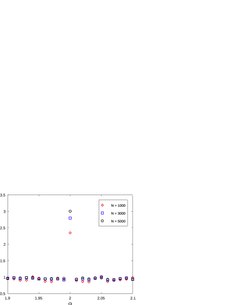
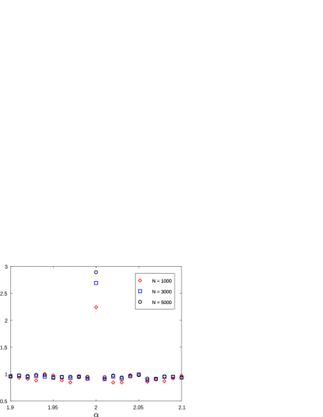
Figure 1. The ordinate of the left (resp. right) figure is the value $\mathcal{N}_{2}^{(1,2)}(N)/N^{3-\alpha}$ (resp. $\mathcal{N}_{2}^{(3)}(N)/N^{3-\alpha}$) divided by the right-hand side of (4.1) (resp. (4.2)), where $N\in\{1000+2000i:i=0,1,2\}$ and $\alpha\in\{1.9+0.01i:i=0,1,\ldots,20\}$.

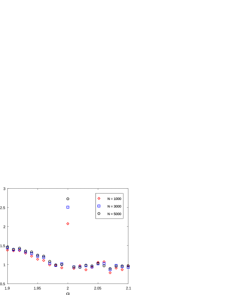
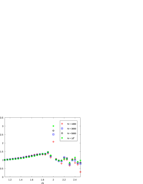
Figure 2. The ordinate of the left (resp. right) figure is the value $\mathcal{N}_{\alpha}^{\mathrm{AP}}(N)/N^{3-\alpha}$ divided by the right-hand side of (4.3), where $N\in\{1000+2000i:i=0,1,2\}$ (resp. $N\in\{1000+2000i:i=0,1,2\}\cup\{10^{4}\}$) and $\alpha\in\{1.9+0.01i:i=0,1,\ldots,20\}$ (resp. $\alpha\in\{1.1+0.05i:i=0,1,\ldots,28\}$).

Now, let us consider the following two statements: for Lebesgue-a.e. $\alpha\in(1,\alpha_{0})$ (resp. $\alpha>\alpha_{0}$), the equation $x+y=z$ has infinitely (resp. at most finitely) many solutions in $\mathrm{PS}(\alpha)$. Saito [21] conjectured $\alpha_{0}=3$ for which the two statements hold. He showed [21, Theorem 1.2] that, for Lebesgue-a.e. $\alpha>3$, the equation $x+y=z$ has at most finitely many solutions in $\mathrm{PS}(\alpha)$. Eqs. (4.1) and (4.2) support his conjecture, since $N^{3-\alpha}$ vanishes or diverges to positive infinity as $N\to\infty$ according to $\alpha>3$ or $\alpha<3$.

Heuristic argument on Conjecture 4.1.

It can easily be checked that

$$\mathcal{N}_{\alpha}^{(1,2)}(N)=\#\left\{(n_{1},n_{2})\in\mathbb{N}^{2}:\begin{array}[]{c}n_{1},n_{2}\leq N^{\alpha},\\ \{-n_{1}^{1/\alpha}\}<\phi_{\alpha}(n_{1}),\ \{-n_{2}^{1/\alpha}\}<\phi_{\alpha}(n_{2}),\\ \{-(n_{1}+n_{2})^{1/\alpha}\}<\phi_{\alpha}(n_{1}+n_{2})\end{array}\right\}$$

in the same way as the proof of Theorem 1.1. Assume that the sequences $(-n_{1}^{1/\alpha})$, $(-n_{2}^{1/\alpha})$, and $\bigl{(}-(n_{1}+n_{2})^{1/\alpha}\bigr{)}$ are “sufficiently” equidistributed modulo $1$ when $n_{1}$ and $n_{2}$ run over all integers in the interval $[1,N^{\alpha}]$. Then

(4.4) $$\begin{split}\mathcal{N}_{\alpha}^{(1,2)}(N)&\sim\sum_{1\leq n_{1},n_{2}\leq N^{\alpha}}\phi_{\alpha}(n_{1})\phi_{\alpha}(n_{2})\phi_{\alpha}(n_{1}+n_{2})\\ &\sim\sum_{1\leq n_{1},n_{2}\leq N^{\alpha}}\alpha^{-3}\bigl{(}n_{1}n_{2}(n_{1}+n_{2})\bigr{)}^{1/\alpha-1}\\ &=N^{3-\alpha}\cdot\frac{\alpha^{-3}}{N^{2\alpha}}\sum_{1\leq n_{1},n_{2}\leq N^{\alpha}}\Bigl{(}\frac{n_{1}}{N^{\alpha}}\cdot\frac{n_{2}}{N^{\alpha}}\cdot\frac{n_{1}+n_{2}}{N^{\alpha}}\Bigr{)}^{1/\alpha-1}\\ &\sim N^{3-\alpha}\cdot\alpha^{-3}\iint_{0<x,y\leq 1}\bigl{(}xy(x+y)\bigr{)}^{1/\alpha-1}\,dxdy\end{split}$$

as $N\to\infty$. Also, assume that the sequences $(-n_{1}^{1/\alpha})$, $(-n_{2}^{1/\alpha})$, and $\bigl{(}-(n_{1}+n_{2})^{1/\alpha}\bigr{)}$ are “sufficiently” equidistributed modulo $1$ when $n_{1}$ and $n_{2}$ run over all positive integers with $n_{1}+n_{2}\leq N^{\alpha}$. Then

(4.5) $$\begin{split}\mathcal{N}_{\alpha}^{(3)}(N)&=\#\left\{(n_{1},n_{2})\in\mathbb{N}^{2}:\begin{array}[]{c}n_{1}+n_{2}\leq N^{\alpha},\\ \{-n_{1}^{1/\alpha}\}<\phi_{\alpha}(n_{1}),\ \{-n_{2}^{1/\alpha}\}<\phi_{\alpha}(n_{2}),\\ \{-(n_{1}+n_{2})^{1/\alpha}\}<\phi_{\alpha}(n_{1}+n_{2})\end{array}\right\}\\ &\sim N^{3-\alpha}\cdot\alpha^{-3}\iint_{\begin{subarray}{c}x,y>0\\ x+y\leq 1\end{subarray}}\bigl{(}xy(x+y)\bigr{)}^{1/\alpha-1}\,dxdy\end{split}$$

as $N\to\infty$. By the change of variables $(x,y)=(u(1-v),uv)$, it turns out that

(4.6) $$\begin{split}&\quad\iint_{\begin{subarray}{c}x,y>0\\ x+y\leq 1\end{subarray}}\bigl{(}xy(x+y)\bigr{)}^{1/\alpha-1}\,dxdy=\iint_{0<u,v\leq 1}\bigl{(}u^{3}(1-v)v\bigr{)}^{1/\alpha-1}u\,dudv\\ &=\int_{0}^{1}u^{3/\alpha-2}\,du\int_{0}^{1}\bigl{(}(1-v)v\bigr{)}^{1/\alpha-1}\,dv=\frac{B(1/\alpha,1/\alpha)}{3/\alpha-1}=\frac{\alpha\Gamma(1/\alpha)^{2}}{(3-\alpha)\Gamma(2/\alpha)}\\ &=\frac{\alpha^{3}\Gamma(1+1/\alpha)^{2}}{(3-\alpha)\Gamma(2/\alpha)}.\end{split}$$

By (4.5) and (4.6), we obtain (4.2). Similarly,

$$\quad\iint_{\begin{subarray}{c}0<x,y\leq 1\\ x+y>1\end{subarray}}\bigl{(}xy(x+y)\bigr{)}^{1/\alpha-1}\,dxdy$$

$$=\int_{1}^{2}u^{3/\alpha-2}\,du\int_{1-1/u}^{1/u}\bigl{(}(1-v)v\bigr{)}^{1/\alpha-1}\,dv=\alpha^{3}I(\alpha).$$

Therefore,

(4.7) $$\alpha^{-3}\iint_{0<x,y\leq 1}\bigl{(}xy(x+y)\bigr{)}^{1/\alpha-1}\,dxdy=\frac{\Gamma(1+1/\alpha)^{2}}{(3-\alpha)\Gamma(2/\alpha)}+I(\alpha).$$

By (4.4) and (4.7), we obtain (4.1). ∎

Heuristic argument on Conjecture 4.2.

Assume that the sequences $(-n_{1}^{1/\alpha})$, $(-n_{2}^{1/\alpha})$, and $\bigl{(}-(2n_{2}-n_{1})^{1/\alpha}\bigr{)}$ are “sufficiently” equidistributed modulo $1$ when $n_{1}$ and $n_{2}$ run over all positive integers with $n_{1}<n_{2}<2n_{2}-n_{1}\leq N^{\alpha}$. Then

(4.8) $$\begin{split}\mathcal{N}_{\alpha}^{\mathrm{AP}}(N)&=\#\left\{(n_{1},n_{2})\in\mathbb{N}^{2}:\begin{array}[]{c}1\leq n_{1}<n_{2}<2n_{2}-n_{1}\leq N^{\alpha},\\ \{-n_{1}^{1/\alpha}\}<\phi_{\alpha}(n_{1}),\ \{-n_{2}^{1/\alpha}\}<\phi_{\alpha}(n_{2}),\\ \{-(2n_{2}-n_{1})^{1/\alpha}\}<\phi_{\alpha}(2n_{2}-n_{1})\end{array}\right\}\\ &\sim N^{3-\alpha}\cdot\alpha^{-3}\iint_{0<x<y<2y-x\leq 1}\bigl{(}xy(2y-x)\bigr{)}^{1/\alpha-1}\,dxdy.\end{split}$$

as $N\to\infty$. By the change of variables $(x,z)=(x,2y-x)$, it turns out that

(4.9) $$\begin{split}&\quad\iint_{0<x<y<2y-x\leq 1}\bigl{(}xy(2y-x)\bigr{)}^{1/\alpha-1}\,dxdy\\ &=2^{-1/\alpha}\iint_{0<x<z\leq 1}\bigl{(}xz(x+z)\bigr{)}^{1/\alpha-1}\,dxdz\\ &=2^{-1/\alpha-1}\iint_{0<x,z\leq 1}\bigl{(}xz(x+z)\bigr{)}^{1/\alpha-1}\,dxdz.\end{split}$$

By (4.8), (4.9), and (4.7), we obtain (4.3). ∎

Appendix A Proof of Theorem 1.5

In this appendix, we prove Theorem 1.5. For this purpose, we begin with the following lemma, which is a simple generalization of [8, pp. 394–395, Fundamental lemma].

Lemma A.1.

Let $\alpha_{1},\alpha_{2}>1$ be real numbers, and $N\geq 2$ be an integer. If a positive integer $n_{1}\leq N^{1/\alpha_{1}}$ satisfies the following two conditions, then there exists a positive integer $n_{2}$ such that $\lfloor{n_{1}^{\alpha_{1}}}\rfloor+\lfloor{n_{2}^{\alpha_{2}}}\rfloor=N$.

1. $1-\{(N+1/2-n_{1}^{\alpha_{1}})^{1/\alpha_{2}}\}\leq(1/2\alpha_{2})(N+1/2)^{1/\alpha_{2}-1}$.

2. $\{n_{1}^{\alpha_{1}}\}<1/2$.

Proof.

Assume that a positive integer $n_{1}\leq N^{1/\alpha_{1}}$ satisfies conditions 1–2. Set $n_{2}=\lfloor{(N+1/2-n_{1}^{\alpha_{1}})^{1/\alpha_{2}}}\rfloor+1$. By condition 1,

(A.1) $$\begin{split}(N+1/2-n_{1}^{\alpha_{1}})^{1/\alpha_{2}}<n_{2}&=(N+1/2-n_{1}^{\alpha_{1}})^{1/\alpha_{2}}+1-\{(N+1/2-n_{1}^{\alpha_{1}})^{1/\alpha_{2}}\}\\ &\leq(N+1/2-n_{1}^{\alpha_{1}})^{1/\alpha_{2}-1}+(1/2\alpha_{2})(N+1/2)^{1/\alpha_{2}-1}.\end{split}$$

The mean value theorem implies that

$$(N+1-n_{1}^{\alpha_{1}})^{1/\alpha_{2}}=(N+1/2-n_{1}^{\alpha_{1}})^{1/\alpha_{2}}+\frac{1}{2\alpha_{2}}(N+1/2-n_{1}^{\alpha_{1}}+\theta)^{1/\alpha_{2}-1}$$

for some $\theta\in(1/2,1)$. By this and $0<N+1/2-n_{1}^{\alpha_{1}}+\theta<N+1/2$, we have

$$(N+1-n_{1}^{\alpha_{1}})^{1/\alpha_{2}}>(N+1/2-n_{1}^{\alpha_{1}})^{1/\alpha_{2}}+(1/2\alpha_{2})(N+1/2)^{1/\alpha_{2}-1}.$$

This and (A.1) yield that

$$(N+1/2-n_{1}^{\alpha_{1}})^{1/\alpha_{2}}<n_{2}<(N+1-n_{1}^{\alpha_{1}})^{1/\alpha_{2}},$$

which is equivalent to

$$N+1/2<n_{1}^{\alpha_{1}}+n_{2}^{\alpha_{2}}<N+1.$$

By condition 2,

$$N+1 >\lfloor{n_{1}^{\alpha_{1}}}\rfloor+\lfloor{n_{2}^{\alpha_{2}}}\rfloor=n_{1}^{\alpha_{1}}+n_{2}^{\alpha_{2}}-\{n_{1}^{\alpha_{1}}\}-\{n_{2}^{\alpha_{2}}\}$$

$$>(N+1/2)-1/2-1=N-1.$$

Therefore, $\lfloor{n_{1}^{\alpha_{1}}}\rfloor+\lfloor{n_{2}^{\alpha_{2}}}\rfloor=N$. ∎

An outline of the proof of Theorem 1.5 is as follows. By Lemmas A.1 and 2.1, Theorem 1.5 reduces to estimating exponential sums. To estimate exponential sums, we use Lemmas 2.3, 2.4, and 2.5. Although Deshouillers [8] used the third derivative test of van der Corput, we use Lemma 2.4 instead.

Proof of Theorem 1.5.

Without loss of generality, we may assume that $1<\alpha_{1}\leq\alpha_{2}<3/2$. Let $N\geq e^{4}-1/2$ be an integer. Set $c_{1}=1/2$, $c_{2}=3/4$, $X=N+1/2$,

(A.2) $$H_{1}=\log X\quad\text{and}\quad H_{2}=X^{1-1/\alpha_{2}}\log X.$$

Then both $H_{1}$ and $H_{2}$ are greater than or equal to $4$. Lemma 2.1 implies that the value

$$R =\#\biggl{\{}(c_{1}X)^{1/\alpha_{1}}\leq n\leq(c_{2}X)^{1/\alpha_{1}}:\begin{array}[]{c}\{n^{\alpha_{1}}\}<1/2,\\ 1-\{(X-n^{\alpha_{1}})^{1/\alpha_{2}}\}\leq(1/2\alpha_{2})X^{1/\alpha_{2}-1}\end{array}\biggr{\}}$$

$$\quad-\frac{c_{2}^{1/\alpha_{1}}-c_{1}^{1/\alpha_{1}}}{4\alpha_{2}}X^{1/\alpha_{1}+1/\alpha_{2}-1}$$

satisfies the inequality

$$R\ll R_{0}+R_{3}+R_{2,1}+R_{2,2}+R_{1},$$

where $f_{1}(x)=x^{\alpha_{1}}$, $f_{2}(x)=(X-x^{\alpha_{1}})^{1/\alpha_{2}}$, $\mathcal{I}=[(c_{1}X)^{1/\alpha_{1}},(c_{2}X)^{1/\alpha_{1}}]$,

$$R_{0}=\left|(c_{2}^{1/\alpha_{1}}-c_{1}^{1/\alpha_{1}})X^{1/\alpha_{1}}-\#(\mathcal{I}\cap\mathbb{Z})\right|X^{1/\alpha_{2}-1},$$

$$R_{3}=\sum_{\begin{subarray}{c}1\leq\left|h_{1}\right|\leq H_{1}\\ 1\leq\left|h_{2}\right|\leq H_{2}\end{subarray}}\left|h_{1}\right|^{-1}\min\{X^{1/\alpha_{2}-1},\left|h_{2}\right|^{-1}\}\left|\sum_{n\in\mathcal{I}\cap\mathbb{Z}}e\bigl{(}h_{1}f_{1}(n)+h_{2}f_{2}(n)\bigr{)}\right|,$$

$$R_{2,1}=X^{1/\alpha_{2}-1}\sum_{1\leq h\leq H_{1}}h^{-1}\left|\sum_{n\in\mathcal{I}\cap\mathbb{Z}}e\bigl{(}hf_{1}(n)\bigr{)}\right|,$$

$$R_{2,2}=\sum_{1\leq h\leq H_{2}}\min\{X^{1/\alpha_{2}-1},h^{-1}\}\left|\sum_{n\in\mathcal{I}\cap\mathbb{Z}}e\bigl{(}hf_{2}(n)\bigr{)}\right|,\quad\text{and}$$

$$R_{1}=X^{1/\alpha_{1}}\Bigl{(}\frac{1}{H_{2}}+\frac{X^{1/\alpha_{2}-1}}{H_{1}}\Bigr{)}.$$

Also, partition the sum $R_{3}$ into two sums:

$$R_{3}=\sum_{\begin{subarray}{c}1\leq\left|h_{1}\right|\leq H_{1}\\ 1\leq\left|h_{2}\right|\leq H_{2}\end{subarray}}=\sum_{\begin{subarray}{c}1\leq\left|h_{1}\right|\leq H_{1}\\ 1\leq\left|h_{2}\right|\leq H_{2}\\ h_{1}h_{2}>0\end{subarray}}+\sum_{\begin{subarray}{c}1\leq\left|h_{1}\right|\leq H_{1}\\ 1\leq\left|h_{2}\right|\leq H_{2}\\ h_{1}h_{2}<0\end{subarray}}=R_{3,1}+R_{3,2},\quad\text{say}.$$

If $R=o(X^{1/\alpha_{1}+1/\alpha_{2}-1})$ as $X\to\infty$, then $\mathcal{R}_{\alpha_{1},\alpha_{2}}(N)\gg N^{1/\alpha_{1}+1/\alpha_{2}-1}$ as $N\to\infty$ due to Lemma A.1. Hence, we show that $R=o(X^{1/\alpha_{1}+1/\alpha_{2}-1})$ below.

Step 1. By (A.2), it is clear that

$$R_{0}\leq X^{1/\alpha_{2}-1}\quad\text{and}\quad R_{1}\ll X^{1/\alpha_{1}+1/\alpha_{2}-1}(\log X)^{-1}.$$

Also, $\left|f^{\prime}_{1}(x)\right|\asymp_{\alpha_{1}}X^{1-1/\alpha_{1}}$ when $x\in\mathcal{I}$. Using the exponent pair $(1/2,1/2)$ (see Lemma 2.5), we have

$$\sum_{n\in\mathcal{I}\cap\mathbb{Z}}e\bigl{(}hf_{1}(n)\bigr{)} \ll_{\alpha_{1}}(hX^{1-1/\alpha_{1}})^{1/2}(X^{1/\alpha_{1}})^{1/2}+(hX^{1-1/\alpha_{1}})^{-1}$$

$$=h^{1/2}X^{1/2}+h^{-1}X^{1/\alpha_{1}-1}\ll h^{1/2}X^{1/2}$$

for every $h\geq 1$. Thus,

$$\sum_{1\leq h\leq H_{1}}h^{-1}\left|\sum_{n\in\mathcal{I}\cap\mathbb{Z}}e\bigl{(}hf_{1}(n)\bigr{)}\right| \ll_{\alpha_{1}}\sum_{1\leq h\leq H_{1}}h^{-1}\cdot h^{1/2}X^{1/2}$$

$$\ll H_{1}^{1/2}X^{1/2}=X^{1/2}(\log X)^{1/2},$$

where we have used (A.2) to obtain the last equality. Therefore,

$$R_{2,1}\ll_{\alpha_{1}}X^{1/\alpha_{2}-1/2}(\log X)^{1/2}.$$

Step 2. The first and second derivatives $f^{\prime}_{2}$ and $f^{\prime\prime}_{2}$ of $f_{2}$ are below:

(A.3) $$f^{\prime}_{2}(x) =-\alpha_{1}\alpha_{2}^{-1}x^{\alpha_{1}-1}(X-x^{\alpha_{1}})^{1/\alpha_{2}-1},$$

(A.4) $$\begin{split}f^{\prime\prime}_{2}(x)&=-\alpha_{1}\alpha_{2}^{-1}\bigl{(}(\alpha_{1}-1)X+(1-\alpha_{1}\alpha_{2}^{-1})x^{\alpha_{1}}\bigr{)}x^{\alpha_{1}-2}(X-x^{\alpha_{1}})^{1/\alpha_{2}-2}\\ &=\bigl{(}(\alpha_{1}-1)X+(1-\alpha_{1}\alpha_{2}^{-1})x^{\alpha_{1}}\bigr{)}x^{-1}(X-x^{\alpha_{1}})^{-1}f^{\prime}_{2}(x).\end{split}$$

When $x\in\mathcal{I}$, we have $\left|f^{\prime\prime}_{2}(x)\right|\asymp_{\alpha_{1},\alpha_{2}}X^{1/\alpha_{2}-2/\alpha_{1}}$. This and Lemma 2.3 imply that

$$\sum_{n\in\mathcal{I}\cap\mathbb{Z}}e\bigl{(}hf_{2}(n)\bigr{)} \ll_{\alpha_{1},\alpha_{2}}X^{1/\alpha_{1}}(hX^{1/\alpha_{2}-2/\alpha_{1}})^{1/2}+(hX^{1/\alpha_{2}-2/\alpha_{1}})^{-1/2}$$

$$=h^{1/2}X^{1/2\alpha_{2}}+h^{-1/2}X^{1/\alpha_{1}-1/2\alpha_{2}}$$

for every $h\geq 1$. Therefore,

$$R_{2,2} \ll_{\alpha_{1},\alpha_{2}}\sum_{1\leq h\leq H_{2}}\min\{X^{1/\alpha_{2}-1},h^{-1}\}(h^{1/2}X^{1/2\alpha_{2}}+h^{-1/2}X^{1/\alpha_{1}-1/2\alpha_{2}})$$

$$\leq\sum_{1\leq h\leq H_{2}}(h^{-1}\cdot h^{1/2}X^{1/2\alpha_{2}}+X^{1/\alpha_{2}-1}\cdot h^{-1/2}X^{1/\alpha_{1}-1/2\alpha_{2}})$$

$$\ll H_{2}^{1/2}X^{1/2\alpha_{2}}+H_{2}^{1/2}X^{1/\alpha_{1}+1/2\alpha_{2}-1}$$

$$\ll H_{2}^{1/2}X^{1/2\alpha_{2}}=X^{1/2}(\log X)^{1/2},$$

where we have used (A.2) to obtain the last equality.

Step 3. Let $h_{1}h_{2}<0$. From now on, set $f=h_{1}f_{1}+h_{2}f_{2}$. When $x\in\mathcal{I}$, we have

$$\left|f^{\prime\prime}(x)\right|\asymp_{\alpha_{1},\alpha_{2}}\left|h_{1}\right|X^{1-2/\alpha_{1}}+\left|h_{2}\right|X^{1/\alpha_{2}-2/\alpha_{1}}.$$

This and Lemma 2.3 imply that

$$\sum_{n\in\mathcal{I}\cap\mathbb{Z}}e\bigl{(}f(n)\bigr{)} \ll_{\alpha_{1},\alpha_{2}}X^{1/\alpha_{1}}(\left|h_{1}\right|^{1/2}X^{1/2-1/\alpha_{1}}+\left|h_{2}\right|^{1/2}X^{1/2\alpha_{2}-1/\alpha_{1}})$$

$$\qquad\qquad+\min\{\left|h_{1}\right|^{-1/2}X^{1/\alpha_{1}-1/2},\left|h_{2}\right|^{-1/2}X^{1/\alpha_{1}-1/2\alpha_{2}}\}$$

$$\leq\left|h_{1}\right|^{1/2}X^{1/2}+\left|h_{2}\right|^{1/2}X^{1/2\alpha_{2}}+\left|h_{2}\right|^{-1/2}X^{1/\alpha_{1}-1/2\alpha_{2}}.$$

Thus,

$$R_{3,2} \ll_{\alpha_{1},\alpha_{2}}\sum_{\begin{subarray}{c}1\leq h_{1}\leq H_{1}\\ 1\leq h_{2}\leq H_{2}\end{subarray}}\left|h_{1}\right|^{-1}\min\{X^{1/\alpha_{2}-1},\left|h_{2}\right|^{-1}\}$$

$$\qquad\qquad\qquad(\left|h_{1}\right|^{1/2}X^{1/2}+\left|h_{2}\right|^{1/2}X^{1/2\alpha_{2}}+\left|h_{2}\right|^{-1/2}X^{1/\alpha_{1}-1/2\alpha_{2}}).$$

By the inequalities

$$\left|h_{1}\right|^{-1}\min\{X^{1/\alpha_{2}-1},\left|h_{2}\right|^{-1}\}\leq\left|h_{1}\right|^{-1}\left|h_{2}\right|^{-1},\ \left|h_{1}\right|^{-1}X^{1/\alpha_{2}-1},$$

it turns out that

$$R_{3,2} \ll_{\alpha_{1},\alpha_{2}}\sum_{\begin{subarray}{c}1\leq h_{1}\leq H_{1}\\ 1\leq h_{2}\leq H_{2}\end{subarray}}\bigl{(}h_{1}^{-1}h_{2}^{-1}(\left|h_{1}\right|^{1/2}X^{1/2}+\left|h_{2}\right|^{1/2}X^{1/2\alpha_{2}})$$

$$\qquad\qquad\qquad+h_{1}^{-1}X^{1/\alpha_{2}-1}\cdot\left|h_{2}\right|^{-1/2}X^{1/\alpha_{1}-1/2\alpha_{2}}\bigr{)}$$

$$\ll H_{1}^{1/2}(\log H_{2})X^{1/2}+(\log H_{1})H_{2}^{1/2}X^{1/2\alpha_{2}}$$

$$\quad+(\log H_{1})H_{2}^{1/2}X^{1/\alpha_{1}+1/2\alpha_{2}-1}$$

$$\ll_{\alpha_{2}}X^{1/2}(\log X)^{3/2}+X^{1/2}(\log X)^{1/2}(\log\log X)$$

$$\quad+X^{1/\alpha_{1}-1/2}(\log X)^{1/2}(\log\log X)$$

$$\ll X^{1/2}(\log X)^{3/2},$$

where we have used (A.2) to obtain the second to last inequality.

Step 4. Let $h_{1}h_{2}>0$. When $x\in\mathcal{I}$, we have

(A.5) $$\left|f^{\prime\prime}_{1}(x)\right|\asymp_{\alpha_{1}}X^{1-2/\alpha_{1}}\quad\text{and}\quad\left|f^{\prime\prime}_{2}(x)\right|\asymp_{\alpha_{1},\alpha_{2}}X^{1/\alpha_{2}-2/\alpha_{1}}.$$

Take a small $\delta_{2}=\delta_{2}(\alpha_{1},\alpha_{2})\in(0,1)$ such that if $\left|h_{2}\right|\leq\delta_{2}X^{1-1/\alpha_{2}}$ and $x\in\mathcal{I}$, then

(A.6) $$\left|f^{\prime\prime}(x)\right|=\left|h_{1}f^{\prime\prime}_{1}(x)\right|-\left|h_{2}f^{\prime\prime}_{2}(x)\right|\asymp_{\alpha_{1},\alpha_{2}}\left|h_{1}\right|X^{1-2/\alpha_{1}}.$$

(Note that $h_{1}$ is a non-zero integer.) If $\left|h_{2}\right|\leq\delta_{2}X^{1-1/\alpha_{2}}$, Lemma 2.3 and (A.6) imply that

$$\sum_{n\in\mathcal{I}\cap\mathbb{Z}}e\bigl{(}f(n)\bigr{)} \ll_{\alpha_{1},\alpha_{2}}X^{1/\alpha_{1}}(\left|h_{1}\right|X^{1-2/\alpha_{1}})^{1/2}+(\left|h_{1}\right|X^{1-2/\alpha_{1}})^{-1/2}$$

$$=\left|h_{1}\right|^{1/2}X^{1/2}+\left|h_{1}\right|^{-1/2}X^{1/\alpha_{1}-1/2}\ll\left|h_{1}\right|^{1/2}X^{1/2}.$$

This yields that

$$R_{3,1,1} \coloneqq\sum_{\begin{subarray}{c}1\leq\left|h_{1}\right|\leq H_{1}\\ 1\leq\left|h_{2}\right|\leq\delta_{2}X^{1-1/\alpha_{2}}\\ h_{1}h_{2}>0\end{subarray}}\left|h_{1}\right|^{-1}\min\{X^{1/\alpha_{2}-1},\left|h_{2}\right|^{-1}\}\left|\sum_{n\in\mathcal{I}\cap\mathbb{Z}}e\bigl{(}f(n)\bigr{)}\right|$$

$$\ll_{\alpha_{1},\alpha_{2}}\sum_{\begin{subarray}{c}1\leq h_{1}\leq H_{1}\\ 1\leq h_{2}\leq\delta_{2}X^{1-1/\alpha_{2}}\end{subarray}}h_{1}^{-1}X^{1/\alpha_{2}-1}\cdot\left|h_{1}\right|^{1/2}X^{1/2}$$

$$\ll H_{1}^{1/2}\cdot\delta_{2}X^{1-1/\alpha_{2}}\cdot X^{1/\alpha_{2}-1/2}\leq X^{1/2}(\log X)^{1/2},$$

where we have used (A.2) and $\delta_{2}\in(0,1)$ to obtain the last inequality.

Step 5. Now, we investigate the third derivative $f^{\prime\prime\prime}$ of $f$ to estimate

$$R_{3,1,2}\coloneqq\sum_{\begin{subarray}{c}1\leq\left|h_{1}\right|\leq H_{1}\\ \delta_{2}X^{1-1/\alpha_{2}}<\left|h_{2}\right|\leq H_{2}\\ h_{1}h_{2}>0\end{subarray}}\left|h_{1}\right|^{-1}\min\{X^{1/\alpha_{2}-1},\left|h_{2}\right|^{-1}\}\left|\sum_{n\in\mathcal{I}\cap\mathbb{Z}}e\bigl{(}f(n)\bigr{)}\right|.$$

Let $x\in\mathcal{I}$. We show that (i) $f^{\prime\prime\prime}(x)<0$ if $h_{1},h_{2}>0$; (ii) $f^{\prime\prime\prime}(x)>0$ if $h_{1},h_{2}<0$. By (A.4), the third derivative $f^{\prime\prime\prime}_{2}$ of $f_{2}$ is

(A.7) $$\begin{split}f^{\prime\prime\prime}_{2}(x)&=\bigl{(}(\alpha_{1}-1)X+(1-\alpha_{1}\alpha_{2}^{-1})x^{\alpha_{1}}\bigr{)}x^{-1}(X-x^{\alpha_{1}})^{-1}f^{\prime\prime}_{2}(x)\\ &\quad+(1-\alpha_{1}\alpha_{2}^{-1})\alpha_{1}x^{\alpha_{1}-1}\cdot x^{-1}(X-x^{\alpha_{1}})^{-1}f^{\prime}_{2}(x)\\ &\quad+\bigl{(}(\alpha_{1}-1)X+(1-\alpha_{1}\alpha_{2}^{-1})x^{\alpha_{1}}\bigr{)}(-x^{-2})(X-x^{\alpha_{1}})^{-1}f^{\prime}_{2}(x)\\ &\quad+\bigl{(}(\alpha_{1}-1)X+(1-\alpha_{1}\alpha_{2}^{-1})x^{\alpha_{1}}\bigr{)}x^{-1}\cdot\alpha_{1}x^{\alpha_{1}-1}(X-x^{\alpha_{1}})^{-2}f^{\prime}_{2}(x).\end{split}$$

By (A.4), the third and fourth lines of the right-hand side of (A.7) are equal to

$$-x^{-1}f^{\prime\prime}_{2}(x)\quad\text{and}\quad\alpha_{1}x^{\alpha_{1}-1}(X-x^{\alpha_{1}})^{-1}f^{\prime\prime}_{2}(x),$$

respectively. Thus, the sum of the first, third, and fourth lines of the right-hand side of (A.7) is equal to

$$\quad\bigl{(}(\alpha_{1}-1)X+(1-\alpha_{1}\alpha_{2}^{-1})x^{\alpha_{1}}\bigr{)}x^{-1}(X-x^{\alpha_{1}})^{-1}f^{\prime\prime}_{2}(x)$$

$$\quad-x^{-1}f^{\prime\prime}_{2}(x)+\alpha_{1}x^{\alpha_{1}-1}(X-x^{\alpha_{1}})^{-1}f^{\prime\prime}_{2}(x)$$

$$=\bigl{(}(\alpha_{1}-2)X+(2+\alpha_{1}-\alpha_{1}\alpha_{2}^{-1})x^{\alpha_{1}}\bigr{)}x^{-1}(X-x^{\alpha_{1}})^{-1}f^{\prime\prime}_{2}(x).$$

By this and (A.7),

(A.8) $$\begin{split}f^{\prime\prime\prime}_{2}(x)&=\bigl{(}(\alpha_{1}-2)X+(2+\alpha_{1}-\alpha_{1}\alpha_{2}^{-1})x^{\alpha_{1}}\bigr{)}x^{-1}(X-x^{\alpha_{1}})^{-1}f^{\prime\prime}_{2}(x)\\ &\quad+(1-\alpha_{1}\alpha_{2}^{-1})\alpha_{1}x^{\alpha_{1}-2}(X-x^{\alpha_{1}})^{-1}f^{\prime}_{2}(x).\end{split}$$

By $c_{1}=1/2$, we have

(A.9) $$\begin{split}&\quad(\alpha_{1}-2)X+(2+\alpha_{1}-\alpha_{1}\alpha_{2}^{-1})x^{\alpha_{1}}\\ &\geq(\alpha_{1}-2)X+(2+\alpha_{1}-\alpha_{1}\alpha_{2}^{-1})c_{1}X\\ &=(-2+3\alpha_{1}-\alpha_{1}\alpha_{2}^{-1})X/2\\ &\geq(3\alpha_{1}-3)X/2>0.\end{split}$$

Also, by (A.3) and (A.4), both $f^{\prime}_{2}(x)$ and $f^{\prime\prime}_{2}(x)$ are negative. From this, (A.8), and (A.9), it follows that $f^{\prime\prime\prime}_{2}(x)<0$. Thus, if $h_{1},h_{2}>0$ (resp. $h_{1},h_{2}<0$), then both $h_{1}f^{\prime\prime\prime}_{1}(x)$ and $h_{2}f^{\prime\prime\prime}_{2}(x)$ are negative (resp. positive), which implies that $f^{\prime\prime\prime}(x)<0$ (resp. $f^{\prime\prime\prime}(x)>0$).

Step 6. We calculate and estimate $f^{\prime\prime\prime}(x)-(\alpha_{1}-2)x^{-1}f^{\prime\prime}(x)$. By (A.4) and (A.8),

$$\quad f^{\prime\prime\prime}_{2}(x)-(\alpha_{1}-2)x^{-1}f^{\prime\prime}_{2}(x)$$

$$=(2\alpha_{1}-\alpha_{1}\alpha_{2}^{-1})x^{\alpha_{1}}x^{-1}(X-x^{\alpha_{1}})^{-1}f^{\prime\prime}_{2}(x)$$

$$\quad+(1-\alpha_{1}\alpha_{2}^{-1})\alpha_{1}x^{\alpha_{1}-2}(X-x^{\alpha_{1}})^{-1}f^{\prime}_{2}(x)$$

$$=\Bigl{(}(2\alpha_{1}-\alpha_{1}\alpha_{2}^{-1})x^{\alpha_{1}-1}(X-x^{\alpha_{1}})^{-1}$$

$$\qquad+\frac{(1-\alpha_{1}\alpha_{2}^{-1})\alpha_{1}x^{\alpha_{1}-1}}{(\alpha_{1}-1)X+(1-\alpha_{1}\alpha_{2}^{-1})x^{\alpha_{1}}}\Bigr{)}f^{\prime\prime}_{2}(x).$$

Thus,

(A.10) $$\begin{split}&\quad f^{\prime\prime\prime}(x)-(\alpha_{1}-2)x^{-1}f^{\prime\prime}(x)=h_{2}\bigl{(}f^{\prime\prime\prime}_{2}(x)-(\alpha_{1}-2)x^{-1}f^{\prime\prime}_{2}(x)\bigr{)}\\ &=\Bigl{(}(2\alpha_{1}-\alpha_{1}\alpha_{2}^{-1})x^{\alpha_{1}-1}(X-x^{\alpha_{1}})^{-1}\\ &\qquad+\frac{(1-\alpha_{1}\alpha_{2}^{-1})\alpha_{1}x^{\alpha_{1}-1}}{(\alpha_{1}-1)X+(1-\alpha_{1}\alpha_{2}^{-1})x^{\alpha_{1}}}\Bigr{)}h_{2}f^{\prime\prime}_{2}(x).\end{split}$$

By (A.10) and (A.5),

(A.11) $$\left|f^{\prime\prime\prime}(x)-(\alpha_{1}-2)x^{-1}f^{\prime\prime}(x)\right|\asymp_{\alpha_{1},\alpha_{2}}\left|h_{2}\right|X^{1/\alpha_{2}-3/\alpha_{1}}$$

for every $x\in\mathcal{I}$.

Step 7. Let $h_{1}h_{2}>0$ and $\delta_{2}X^{1-1/\alpha_{2}}<\left|h_{2}\right|\leq H_{2}$. By (A.11), we can take a small $\delta_{0}=\delta_{0}(\alpha_{1},\alpha_{2},\delta_{2})\in(0,1)$ such that if $x\in\mathcal{I}$ and $\left|f^{\prime\prime}(x)\right|\leq\delta_{0}X^{1-2/\alpha_{1}}$, then

$$\left|f^{\prime\prime\prime}(x)\right| \geq\left|f^{\prime\prime\prime}(x)-(\alpha_{1}-2)x^{-1}f^{\prime\prime}(x)\right|-\left|(\alpha_{1}-2)x^{-1}f^{\prime\prime}(x)\right|$$

$$\gg_{\alpha_{1},\alpha_{2},\delta_{2},\delta_{0}}\left|h_{2}\right|X^{1/\alpha_{2}-3/\alpha_{1}}.$$

Also, if $x\in\mathcal{I}$ and $\left|f^{\prime\prime}(x)\right|\leq\delta_{0}X^{1-2/\alpha_{1}}$, then

$$\left|f^{\prime\prime\prime}(x)\right| \leq\left|f^{\prime\prime\prime}(x)-(\alpha_{1}-2)x^{-1}f^{\prime\prime}(x)\right|+\left|(\alpha_{1}-2)x^{-1}f^{\prime\prime}(x)\right|$$

$$\ll_{\alpha_{1},\alpha_{2}}\left|h_{2}\right|X^{1/\alpha_{2}-3/\alpha_{1}}+X^{1-3/\alpha_{1}}\ll_{\delta_{2}}\left|h_{2}\right|X^{1/\alpha_{2}-3/\alpha_{1}}$$

due to (A.11) and $\delta_{0}\in(0,1)$.

Step 8. By $\alpha_{1},\alpha_{2}\in(1,2)$ and $1/\alpha_{1}+6/\alpha_{2}>13/3$, the inequality

$$\max\{0,7/6-1/2\alpha_{1}-1/\alpha_{2}\}<\min\{1/\alpha_{1},2/\alpha_{2}-1\}$$

holds. Indeed, the inequality $7/6-1/2\alpha_{1}-1/\alpha_{2}<1/\alpha_{1}$ follows from

$$3/\alpha_{1}+2/\alpha_{2}=(1/3)(1/\alpha_{1}+6/\alpha_{2})+8/3\alpha_{1}>13/9+4/3=25/3>7/3;$$

the inequality $7/6-1/2\alpha_{1}-1/\alpha_{2}<2/\alpha_{2}-1$ follows from $1/\alpha_{1}+6/\alpha_{2}>13/3$; the other inequalities are trivial. Also, take a real number $c_{0}$ with

(A.12) $$\max\{0,7/6-1/2\alpha_{1}-1/\alpha_{2}\}<c_{0}<\min\{1/\alpha_{1},2/\alpha_{2}-1\},$$

and an integer $m\geq 2$ with

(A.13) $$1/\alpha_{1}+1/\alpha_{2}>3/2+2\cdot 4^{-m}c_{0}.$$

Step 9. Let $h_{1}h_{2}>0$ and $\delta_{2}X^{1-1/\alpha_{2}}<\left|h_{2}\right|\leq H_{2}$. Define the positive numbers $\gamma_{1}<\cdots<\gamma_{m}<1/\alpha_{1}$ as $\gamma_{k}=4^{k-m}c_{0}$. Partition the interval $\mathcal{I}$ into the following subsets $\mathcal{I}_{1},\ldots,\mathcal{I}_{m+1}$:

$$\mathcal{I}_{1} =\{x\in\mathcal{I}:\left|f^{\prime\prime}(x)\right|>\delta_{0}X^{1-2/\alpha_{1}-\gamma_{1}}\},$$

$$\mathcal{I}_{k} =\{x\in\mathcal{I}:\delta_{0}X^{1-2/\alpha_{1}-\gamma_{k}}<\left|f^{\prime\prime}(x)\right|\leq\delta_{0}X^{1-2/\alpha_{1}-\gamma_{k-1}}\}\quad(2\leq k\leq m),$$

$$\mathcal{I}_{m+1} =\{x\in\mathcal{I}:\left|f^{\prime\prime}(x)\right|\leq\delta_{0}X^{1-2/\alpha_{1}-\gamma_{m}}\}.$$

Since $f^{\prime\prime}$ is monotone due to step 5, for $k=1,\ldots,m+1$, the set $\mathcal{I}_{k}$ is a union of at most two intervals. Moreover, for every integer $2\leq k\leq m+1$,

(A.14) $$\left|\mathcal{I}_{k}\right|\ll_{\alpha_{1},\alpha_{2},\delta_{2},\delta_{0}}\left|h_{2}\right|^{-1}X^{1+1/\alpha_{1}-1/\alpha_{2}-\gamma_{k-1}}.$$

Indeed, if $2\leq k\leq m+1$ and $x_{1},x_{2}\in\mathcal{I}_{k}$, then the mean value theorem and step 7 imply that

$$2\delta_{0}X^{1-2/\alpha_{1}-\gamma_{k-1}} \geq\left|f^{\prime\prime}(x_{2})-f^{\prime\prime}(x_{1})\right|=\left|f^{\prime\prime\prime}(x_{3})(x_{2}-x_{1})\right|$$

$$\gg_{\alpha_{1},\alpha_{2},\delta_{2},\delta_{0}}\left|h_{2}\right|X^{1/\alpha_{2}-3/\alpha_{1}}\left|x_{2}-x_{1}\right|$$

for some $x_{3}$ between $x_{1}$ and $x_{2}$ inclusive; therefore,

$$\left|x_{2}-x_{1}\right|\ll_{\alpha_{1},\alpha_{2},\delta_{2},\delta_{0}}\left|h_{2}\right|^{-1}X^{1+1/\alpha_{1}-1/\alpha_{2}-\gamma_{k-1}}.$$

Step 10. Let $h_{1}h_{2}>0$ and $\delta_{2}X^{1-1/\alpha_{2}}<\left|h_{2}\right|\leq H_{2}$. Define the sums $R_{3,1,2,k}$, $k=1,\ldots,m+1$, as

$$R_{3,1,2,k}=\sum_{\begin{subarray}{c}1\leq\left|h_{1}\right|\leq H_{1}\\ \delta_{2}X^{1-1/\alpha_{2}}<\left|h_{2}\right|\leq H_{2}\\ h_{1}h_{2}>0\end{subarray}}\left|h_{1}\right|^{-1}\min\{X^{1/\alpha_{2}-1},\left|h_{2}\right|^{-1}\}\left|\sum_{n\in\mathcal{I}_{k}\cap\mathbb{Z}}e\bigl{(}f(n)\bigr{)}\right|.$$

Then

(A.15) $$R_{3,1,2}\leq\sum_{k=1}^{m+1}R_{3,1,2,k}.$$

First, we estimate $R_{3,1,2,m+1}$. By step 7,

(A.16) $$\left|f^{\prime\prime\prime}(x)\right|\asymp_{\alpha_{1},\alpha_{2},\delta_{2},\delta_{0}}\left|h_{2}\right|X^{1/\alpha_{2}-3/\alpha_{1}}$$

for every $x\in\mathcal{I}_{m+1}$. Lemma 2.4, (A.16), and (A.14) imply that

$$\sum_{n\in\mathcal{I}_{m+1}\cap\mathbb{Z}}e\bigl{(}f(n)\bigr{)} \ll_{\alpha_{1},\alpha_{2},\delta_{2},\delta_{0}}\left|h_{2}\right|^{-1}X^{1+1/\alpha_{1}-1/\alpha_{2}-\gamma_{m}}(\left|h_{2}\right|X^{1/\alpha_{2}-3/\alpha_{1}})^{1/6}$$

$$\qquad\qquad\qquad+(\left|h_{2}\right|X^{1/\alpha_{2}-3/\alpha_{1}})^{-1/3}$$

$$=\left|h_{2}\right|^{-5/6}X^{1+1/2\alpha_{1}-5/6\alpha_{2}-\gamma_{m}}+\left|h_{2}\right|^{-1/3}X^{1/\alpha_{1}-1/3\alpha_{2}}.$$

Thus,

$$R_{3,1,2,m+1} \ll_{\alpha_{1},\alpha_{2},\delta_{2},\delta_{0}}\sum_{\begin{subarray}{c}1\leq h_{1}\leq H_{1}\\ \delta_{2}X^{1-1/\alpha_{2}}<h_{2}\leq H_{2}\end{subarray}}h_{1}^{-1}h_{2}^{-1}(\left|h_{2}\right|^{-5/6}X^{1+1/2\alpha_{1}-5/6\alpha_{2}-\gamma_{m}}$$

$$\qquad\qquad\qquad\qquad\qquad\qquad\qquad\qquad+\left|h_{2}\right|^{-1/3}X^{1/\alpha_{1}-1/3\alpha_{2}})$$

$$\ll_{\delta_{2}}(\log H_{1})\Bigl{(}(X^{1-1/\alpha_{2}})^{-5/6}X^{1+1/2\alpha_{1}-5/6\alpha_{2}-\gamma_{m}}$$

$$\qquad\qquad\qquad\qquad\qquad+(X^{1-1/\alpha_{2}})^{-1/3}X^{1/\alpha_{1}-1/3\alpha_{2}}\Bigr{)}$$

$$=(X^{1/6+1/2\alpha_{1}-\gamma_{m}}+X^{1/\alpha_{1}-1/3})\log\log X,$$

where we have used (A.2) to obtain the last equality. By $\gamma_{m}=c_{0}$, $c_{0}>7/6-1/2\alpha_{1}-1/\alpha_{2}$ of (A.12), and $\alpha_{2}\in(1,3/2)$, it turns out that $R_{3,1,2,m+1}=o(X^{1/\alpha_{1}+1/\alpha_{2}-1})$ as $X\to\infty$.

Next, we estimate $R_{3,1,2,1}$. By (A.5),

(A.17) $$\delta_{0}X^{1-2/\alpha_{1}-\gamma_{1}}\leq\left|f^{\prime\prime}(x)\right|\ll_{\alpha_{1},\alpha_{2}}X^{1-2/\alpha_{2}}\log X$$

for every $x\in\mathcal{I}_{1}$. Lemma 2.3, (A.17), and $\left|\mathcal{I}_{1}\right|\leq\left|\mathcal{I}\right|\ll X^{1/\alpha_{1}}$ imply that

$$\sum_{n\in\mathcal{I}_{1}\cap\mathbb{Z}}e\bigl{(}f(n)\bigr{)} \ll_{\alpha_{1},\alpha_{2},\delta_{0}}X^{1/\alpha_{1}}\cdot\frac{X^{1-2/\alpha_{1}}\log X}{X^{1/2-1/\alpha_{1}-\gamma_{1}/2}}+X^{1/\alpha_{1}-1/2+\gamma_{1}/2}$$

$$=X^{1/2+\gamma_{1}/2}\log X+X^{1/\alpha_{1}-1/2+\gamma_{1}/2}.$$

Thus,

$$R_{3,1,2,1} \ll_{\alpha_{1},\alpha_{2},\delta_{0}}\sum_{\begin{subarray}{c}1\leq h_{1}\leq H_{1}\\ \delta_{2}X^{1-1/\alpha_{2}}<h_{2}\leq H_{2}\end{subarray}}h_{1}^{-1}h_{2}^{-1}(X^{1/2+\gamma_{1}/2}\log X+X^{1/\alpha_{1}-1/2+\gamma_{1}/2})$$

$$\ll(\log H_{1})(\log H_{2})(X^{1/2+\gamma_{1}/2}\log X+X^{1/\alpha_{1}-1/2+\gamma_{1}/2})$$

$$\ll_{\alpha_{2}}X^{1/2+\gamma_{1}/2}(\log X)^{2}\log\log X.$$

By $\gamma_{1}=4^{1-m}c_{0}$ and (A.13), it turns out that $R_{3,1,2,1}=o(X^{1/\alpha_{1}+1/\alpha_{2}-1})$ as $X\to\infty$.

Finally, we estimate $R_{3,1,2,k}$ for $k=2,3,\ldots,m$. Let $2\leq k\leq m$ be an integer. Lemma 2.3 and (A.14) imply that

$$\sum_{n\in\mathcal{I}_{k}\cap\mathbb{Z}}e\bigl{(}f(n)\bigr{)} \ll_{\alpha_{1},\alpha_{2},\delta_{2},\delta_{0}}\left|h_{2}\right|^{-1}X^{1+1/\alpha_{1}-1/\alpha_{2}-\gamma_{k-1}}\cdot\frac{X^{1-2/\alpha_{1}-\gamma_{k-1}}}{X^{1/2-1/\alpha_{1}-\gamma_{k}/2}}$$

$$\qquad\qquad\qquad+X^{1/\alpha_{1}-1/2+\gamma_{k}/2}$$

$$=\left|h_{2}\right|^{-1}X^{3/2-1/\alpha_{2}}+X^{1/\alpha_{1}-1/2+\gamma_{k}/2},$$

where we have used $\gamma_{k}=4\gamma_{k-1}$ to obtain the last equality. Thus,

$$R_{3,1,2,k} \ll_{\alpha_{1},\alpha_{2},\delta_{2},\delta_{0}}\sum_{\begin{subarray}{c}1\leq h_{1}\leq H_{1}\\ \delta_{2}X^{1-1/\alpha_{2}}<h_{2}\leq H_{2}\end{subarray}}h_{1}^{-1}h_{2}^{-1}(\left|h_{2}\right|^{-1}X^{3/2-1/\alpha_{2}}+X^{1/\alpha_{1}-1/2+\gamma_{k}/2})$$

$$\ll_{\delta_{2}}(\log H_{1})\bigl{(}(X^{1-1/\alpha_{2}})^{-1}X^{3/2-1/\alpha_{2}}+(\log H_{2})X^{1/\alpha_{1}-1/2+\gamma_{k}/2}\bigr{)}$$

$$\ll_{\alpha_{2}}(X^{1/2}+X^{1/\alpha_{1}-1/2+\gamma_{k}/2}\log X)\log\log X.$$

By $\gamma_{1}<\cdots<\gamma_{m}=c_{0}$, $c_{0}<2/\alpha_{2}-1$ of (A.12), and $1/\alpha_{1}+1/\alpha_{2}>3/2$, it turns out that $R_{3,1,2,k}=o(X^{1/\alpha_{1}+1/\alpha_{2}-1})$ as $X\to\infty$.

Step 11. By steps 1–4, all of the values $R_{0}$, $R_{1}$, $R_{2,1}$, $R_{2,2}$, $R_{3,2}$, and $R_{3,1,1}$ are $o(X^{1/\alpha_{1}+1/\alpha_{2}-1})$ as $X\to\infty$. By step 10, for every integer $1\leq k\leq m+1$, the value $R_{3,1,2,k}$ is $o(X^{1/\alpha_{1}+1/\alpha_{2}-1})$ as $X\to\infty$. By (A.15) and $R_{3,1}\leq R_{3,1,1}+R_{3,1,2}$, the value $R_{3,1}$ is also $o(X^{1/\alpha_{1}+1/\alpha_{2}-1})$ as $X\to\infty$. Therefore, $R=o(X^{1/\alpha_{1}+1/\alpha_{2}-1})$ as $X\to\infty$. ∎

References

- [1] Y. Akbal and A. M. Güloğlu. Waring’s problem with Piatetski-Shapiro numbers. Mathematika, 62(2):524–550, 2016.
- [2] Y. Akbal and A. M. Güloğlu. On Waring-Goldbach problem with Piatetski-Shapiro primes. J. Number Theory, 185:80–92, 2018.
- [3] G. I. Arkhipov and A. N. Zhitkov. Waring’s problem with nonintegral exponent. Izv. Akad. Nauk SSSR Ser. Mat., 48(6):1138–1150, 1984.
- [4] E. P. Balanzario, M. Z. Garaev, and R. Zuazua. Exceptional set of a representation with fractional powers. Acta Math. Hungar., 114(1-2):103–115, 2007.
- [5] M. Benito and J. L. Varona. Pythagorean triangles with legs less than . J. Comput. Appl. Math., 143(1):117–126, 2002.
- [6] R. F. Churchhouse. On the representation of an integer as the sum of two fractional powers. Bull. London Math. Soc., 5:111–117, 1973.
- [7] J.-M. Deshouillers. Problème de Waring avec exposants non entiers. Bull. Soc. Math. France, 101:285–295, 1973.
- [8] J.-M. Deshouillers. Un problème binaire en théorie additive. Acta Arith., 25:393–403, 1973/74.
- [9] S. Dimitrov. A Diophantine equation involving special prime numbers. Czechoslovak Math. J., 73(148)(1):151–176, 2023.
- [10] S. W. Graham and G. Kolesnik. van der Corput’s method of exponential sums, volume 126 of London Mathematical Society Lecture Note Series. Cambridge University Press, Cambridge, 1991.
- [11] S. A. Gritsenko. Three additive problems. Izv. Ross. Akad. Nauk Ser. Mat., 56(6):1198–1216, 1992.
- [12] S. A. Gritsenko. On estimates for trigonometric sums with respect to the third derivative. Mat. Zametki, 60(3):383–389, 479, 1996.
- [13] T. A. Hulse, C. I. Kuan, D. Lowry-Duda, and A. Walker. Arithmetic progressions of squares and multiple Dirichlet series. preprint, available at https://arxiv.org/abs/2007.14324, 2020.
- [14] J. F. Koksma. Some theorems on Diophantine inequalities. Scriptum no. 5. Math. Centrum Amsterdam, 1950.
- [15] S. V. Konyagin. An additive problem with fractional powers. Mat. Zametki, 73(4):633–636, 2003.
- [16] A. V. Kumchev. A binary additive equation involving fractional powers. Int. J. Number Theory, 5(2):281–292, 2009.
- [17] M. B. S. Laporta. On a binary problem with prime numbers. Math. Balkanica (N.S.), 13(1-2):119–123, 1999.
- [18] Y. R. Listratenko. Estimation of the number of summands in Waring’s problem for the integer parts of fixed powers of nonnegative numbers. volume 3, pages 71–77. 2002. Dedicated to the 85th birthday of Nikolaĭ Mikhaĭlovich Korobov (Russian).
- [19] Zh. Kh. Petrov and D. I. Tolev. On an equation involving fractional powers with one prime and one almost prime variables. Proc. Steklov Inst. Math., 298:S38–S56, 2017.
- [20] G. J. Rieger. On a theorem of Churchhouse concerning sums of fractional powers. Bull. London Math. Soc., 8(2):166–167, 1976.
- [21] K. Saito. Finiteness of solutions to linear Diophantine equations on Piatetski-Shapiro sequences. preprint, available at https://arxiv.org/abs/2306.17813, 2023.
- [22] K. Saito and Y. Yoshida. Distributions of finite sequences represented by polynomials in Piatetski-Shapiro sequences. J. Number Theory, 222:115–156, 2021.
- [23] P. Sargos. Points entiers au voisinage d’une courbe, sommes trigonométriques courtes et paires d’exposants. Proc. London Math. Soc. (3), 70(2):285–312, 1995.
- [24] B. I. Segal. On a theorem analogous to waring’s theorem. Dokl. Akad. Nauk SSSR, 1:47–49, 1933.
- [25] B. I. Segal. Waring’s theorem for powers with fractional and irrational exponents. Tr. Fiz.-Mat. Inst. Steklov. Otdel. Mat., 5:73–86, 1934.
- [26] M. I. Stronina. Integral points on circular cones. Izv. Vysš. Učebn. Zaved. Matematika, 1969(8 (87)):112–116, 1969.
- [27] L. Wu. On an additive problem involving fractional powers with one prime and an almost prime variables. preprint, available at https://arxiv.org/abs/2306.01972, 2023.
- [28] Y. Yoshida. On the number of representations of integers as differences between Piatetski-Shapiro numbers. preprint, available at https://arxiv.org/abs/2103.14239, 2021.
- [29] G. Yu. On a binary additive problem involving fractional powers. J. Number Theory, 208:101–119, 2020.
- [30] L. Zhu. An additive equation involving fractional powers. Acta Math. Hungar., 159(1):174–186, 2019.