Optimal convex $M$-estimation via score matching

Abstract

In the context of linear regression, we construct a data-driven convex loss function with respect to which empirical risk minimisation yields optimal asymptotic variance in the downstream estimation of the regression coefficients. Our semiparametric approach targets the best decreasing approximation of the derivative of the log-density of the noise distribution. At the population level, this fitting process is a nonparametric extension of score matching, corresponding to a log-concave projection of the noise distribution with respect to the Fisher divergence. The procedure is computationally efficient, and we prove that our procedure attains the minimal asymptotic covariance among all convex $M$-estimators. As an example of a non-log-concave setting, for Cauchy errors, the optimal convex loss function is Huber-like, and our procedure yields an asymptotic efficiency greater than $0.87$ relative to the oracle maximum likelihood estimator of the regression coefficients that uses knowledge of this error distribution; in this sense, we obtain robustness without sacrificing much efficiency. Numerical experiments confirm the practical merits of our proposal.

1 Introduction

In linear models, the Gauss–Markov theorem is the primary justification for the use of ordinary least squares (OLS) in settings where the Gaussianity of our error distribution may be in doubt. It states that, provided the errors have a finite second moment, OLS attains the minimal covariance among all linear unbiased estimators; recent papers on this topic include Hansen, (2022), Pötscher and Preinerstorfer, (2022) and Lei and Wooldridge, (2022). Nevertheless, it is now understood that biased, non-linear estimators can achieve lower mean squared error than OLS when the noise distribution is appreciably non-Gaussian (Stein, 1956b, ; Hoerl and Kennard,, 1970; Zou and Yuan,, 2008; Dümbgen et al.,, 2011). However, it remains unclear how best to fit linear models in a computationally efficient and adaptive fashion, i.e. without knowledge of the error distribution.

Consider a linear model where $Y_{i}=X_{i}^{\top}\beta_{0}+\varepsilon_{i}$ for $i=1,\dotsc,n$. Recall that an $M$-estimator of $\beta_{0}\in\mathbb{R}^{d}$ based on a loss function $\ell\colon\mathbb{R}\to\mathbb{R}$ is defined as an empirical risk minimiser

$$\hat{\beta}\in\operatorname*{argmin}_{\beta\in\mathbb{R}^{d}}\frac{1}{n}\sum_{i=1}^{n}\ell(Y_{i}-X_{i}^{\top}\beta),$$ (1)

provided that this exists. If $\ell$ is differentiable on $\mathbb{R}$ with negative derivative $\psi=-\ell^{\prime}$, then $\hat{\beta}\equiv\hat{\beta}_{\psi}$ solves the corresponding estimating equations

$$\frac{1}{n}\sum_{i=1}^{n}X_{i}\psi(Y_{i}-X_{i}^{\top}\hat{\beta}_{\psi})=0$$ (2)

and is referred to as a $Z$-estimator. We study a random design setting in which $(X_{1},Y_{1}),\dotsc,(X_{n},Y_{n})$ are independent and identically distributed, with $X_{1},\dotsc,X_{n}$ being $\mathbb{R}^{d}$-valued covariates that are independent of real-valued errors $\varepsilon_{1},\dotsc,\varepsilon_{n}$ with density $p_{0}$. Suppose further that $\mathbb{E}\{X_{1}\psi(\varepsilon_{1})\}=0$. This means that $\hat{\beta}_{\psi}$ is Fisher consistent in the sense that the population analogue of (2) is satisfied by the true parameter $\beta_{0}$, i.e. $\mathbb{E}\{X_{1}\psi(Y_{1}-X_{1}^{\top}\beta_{0})\}=0$. Under suitable regularity conditions, including $\psi$ being differentiable and $\mathbb{E}(X_{1}X_{1}^{\top})\in\mathbb{R}^{d\times d}$ being invertible, we have

$$\sqrt{n}(\hat{\beta}_{\psi}-\beta_{0})\overset{d}{\to}N_{d}\bigl{(}0,V_{p_{0}}(\psi)\cdot\{\mathbb{E}(X_{1}X_{1}^{\top})\}^{-1}\bigr{)}\quad\text{as }n\to\infty,\quad\text{where }V_{p_{0}}(\psi):=\frac{\mathbb{E}\psi^{2}(\varepsilon_{1})}{\{\mathbb{E}\psi^{\prime}(\varepsilon_{1})\}^{2}}$$ (3)

(e.g. van der Vaart,, 1998, Theorems 5.21, 5.23 and 5.41). Since the covariates and errors are assumed to be independent, they contribute separately to the limiting covariance above (a special case of the ‘sandwich’ formula (Huber,, 1967; Young and Shah,, 2023)): the matrix $\mathbb{E}(X_{1}X_{1}^{\top})^{-1}$ depends only on the covariate distribution, whereas the scalar $V_{p_{0}}(\psi)$ depends on the loss function $\ell$ (through $\psi=-\ell^{\prime}$) and on the error distribution.

If the errors $\varepsilon_{1},\varepsilon_{2},\dotsc$ have a known absolutely continuous density $p_{0}$ on $\mathbb{R}$, then we can define the maximum likelihood estimator $\hat{\beta}^{\mathrm{MLE}}$ by taking $\ell=-\log p_{0}$ in (1). In this case, $\psi=-\ell^{\prime}$ is the score function (for location) $\psi_{0}:=(p_{0}^{\prime}/p_{0})\mathbbm{1}_{\{p_{0}>0\}}$. Under appropriate regularity conditions (e.g. van der Vaart,, 1998, Theorem 5.39), including that the Fisher information (for location) $i(p_{0}):=\int_{\mathbb{R}}\psi_{0}^{2}\,p_{0}=\int_{\{p_{0}>0\}}(p_{0}^{\prime})^{2}/p_{0}$ is finite, we have

$$\sqrt{n}\,(\hat{\beta}^{\mathrm{MLE}}-\beta_{0})\overset{d}{\to}N_{d}\biggl{(}0,\frac{\{\mathbb{E}(X_{1}X_{1}^{\top})\}^{-1}}{i(p_{0})}\biggr{)}$$ (4)

as $n\to\infty$. The limiting covariance $\{\mathbb{E}(X_{1}X_{1}^{\top})\}^{-1}/i(p_{0})$ constitutes an efficiency lower bound; see Remark 15 below. In fact, it can be seen directly that $1/i(p_{0})$ is the smallest possible value of the asymptotic variance factor $V_{p_{0}}(\psi)$ in the limiting covariance of $\sqrt{n}(\hat{\beta}_{\psi}-\beta_{0})$ in (3). Indeed, by the Cauchy–Schwarz inequality,

$$V_{p_{0}}(\psi)=\frac{\int_{\mathbb{R}}\psi^{2}p_{0}}{\bigl{(}\int_{\mathbb{R}}\psi^{\prime}p_{0}\bigr{)}^{2}}=\frac{\int_{\mathbb{R}}\psi^{2}p_{0}}{\bigl{(}\int_{\mathbb{R}}\psi p_{0}^{\prime}\bigr{)}^{2}}\geq\frac{1}{\int_{\{p_{0}>0\}}(p_{0}^{\prime})^{2}/p_{0}}=\frac{1}{i(p_{0})}\in(0,\infty),$$ (5)

whenever the integration by parts in the second step is justified, and equality holds if and only if there exists $\lambda\neq 0$ such that $\psi(\varepsilon_{1})=\lambda\psi_{0}(\varepsilon_{1})$ almost surely. This leads to an equivalent variational definition of the Fisher information; see Huber and Ronchetti, (2009, Theorem 4.2), which we restate as Proposition 36 in Section 6.4. Thus, when (4) holds, $\hat{\beta}^{\mathrm{MLE}}$ has minimal asymptotic covariance among all $Z$-estimators $\hat{\beta}_{\psi}$ for which (3) is valid, with the score function $\psi_{0}$ being the optimal choice of $\psi$.

Our goal in this work is to choose $\psi$ in a data-driven manner, such that the corresponding loss function $\ell$ in (1) is convex, and such that the scale factor $V_{p_{0}}(\psi)$ in the asymptotic covariance (3) of the downstream estimator of $\beta_{0}$ is minimised. Convexity is a particularly convenient property for a loss function, since for the purpose of $M$-estimation, it leads to more tractable theory and computation. Indeed, the empirical risk in (1) becomes convex in $\beta$, so its local minimisers are global minimisers. In particular, when $\ell$ is also differentiable, $\hat{\beta}_{\psi}$ is a $Z$-estimator satisfying (2) if and only if it is an $M$-estimator satisfying (1). The existence, uniqueness and $\sqrt{n}$-consistency of $\hat{\beta}_{\psi}$ are then guaranteed under milder conditions on $\ell$ than for generic loss functions (Yohai and Maronna,, 1979; Maronna and Yohai,, 1981; Portnoy,, 1985; Mammen,, 1989; Arcones,, 1998; He and Shao,, 2000). Furthermore, an important practical advantage is that we can compute $\hat{\beta}_{\psi}$ efficiently using convex optimisation algorithms with guaranteed convergence (Boyd and Vandenberghe,, 2004, Chapter 9).

In view of the discussion above, our first main contribution in Section 2 is to determine the optimal population-level convex loss function in the sense described in the previous paragraph. For a uniformly continuous error density $p_{0}$, this amounts to finding

$$\psi_{0}^{*}\in\operatorname*{argmin}_{\psi\in\Psi_{\downarrow}(p_{0})}V_{p_{0}}(\psi),$$ (6)

where $\Psi_{\downarrow}(p_{0})$ denotes the set of decreasing, right-continuous functions $\psi$ satisfying $\int_{\mathbb{R}}\psi^{2}p_{0}<\infty$. We will actually define the ratio $V_{p_{0}}(\psi)$ in a slightly more general way than in (5) to allow us to handle non-differentiable functions $\psi$. This turns out to be convenient because, for instance, the robust Huber loss $\ell_{K}$ given by

$$\ell_{K}(z):=\begin{cases}z^{2}/2\quad&\text{if }|z|\leq K\\ K|z|-K^{2}/2\quad&\text{if }|z|>K\end{cases}$$ (7)

for $K\in(0,\infty)$ has a non-differentiable negative derivative $\psi_{K}:=-\ell_{K}^{\prime}$ satisfying $\psi_{K}(z)=(-K)\vee(-z)\wedge K$ for $z\in\mathbb{R}$.

In Section 2.1, we show that minimising $V_{p_{0}}(\cdot)$ over $\Psi_{\downarrow}(p_{0})$ is equivalent to minimising the score matching objective

$$D_{p_{0}}(\psi):=\mathbb{E}\bigl{\{}\psi^{2}(\varepsilon_{1})+2\psi^{\prime}(\varepsilon_{1})\bigr{\}},$$ (8)

over $\psi\in\Psi_{\downarrow}(p_{0})$, provided that we take appropriate care in defining this expression when $\psi$ is not absolutely continuous. This observation allows us to obtain an explicit characterisation of the ‘projected’ score function $\psi_{0}^{*}$ in terms of $p_{0}$ and its distribution function $F_{0}$. Indeed, to obtain $\psi_{0}^{*}$ at $z\in\mathbb{R}$, we can first consider $p_{0}\circ F_{0}^{-1}$ (whose domain is $[0,1]$), then compute the right derivative of its least concave majorant, before finally applying the resulting function to $F_{0}(z)$. The negative antiderivative $\ell_{0}^{*}$ of $\psi_{0}^{*}$ is then the optimal convex loss function we seek. An important property is that $\mathbb{E}\psi_{0}^{*}(Y_{1}-X_{1}^{\top}\beta_{0})=0$, which ensures that $\ell_{0}^{*}$ correctly identifies the estimand $\beta_{0}$ on the population level; equivalently, $\hat{\beta}_{\psi_{0}^{*}}$ is Fisher consistent.

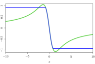
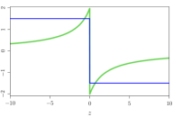
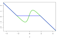
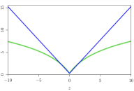
Figure 1: Top row: Plots of the score function $\psi_{0}$ (green) and projected score function $\psi_{0}^{*}$ (blue); Bottom row: their respective negative antiderivatives, namely the negative log-density $-\log p_{0}$ (green) and optimal convex loss function $\ell_{0}^{*}$ (blue), for each of the following non-log-concave distributions (from left to right): (a) Student’s $t_{2}$; (b) symmetrised Pareto (66) with $\sigma=2$ and $\alpha=3$; (c) Gaussian mixture $0.4N(-2,1)+0.6N(2,1)$.

Note that $\hat{\beta}^{\mathrm{MLE}}$ is a convex $M$-estimator if and only if $\ell=-\log p_{0}$ is convex, i.e. $p_{0}$ is log-concave, in which case $\psi_{0}^{*}=\psi_{0}$ by (5). We will be especially interested in error densities $p_{0}$ that are not log-concave, for which the efficiency lower bound in (5) cannot be achieved by a convex $M$-estimator corresponding to a decreasing function $\psi$. We interpret the minimum ratio $V_{p_{0}}(\psi_{0}^{*})$ as an analogue of the inverse Fisher information, serving as the crucial part of the efficiency lower bound for convex $M$-estimators. To reinforce the link with score matching, we will see in Section 2.2 that the density proportional to $e^{-\ell_{0}^{*}}$ is the best log-concave approximation to $p_{0}$ with respect to the Fisher divergence defined formally in (20) below. This is typically different from the well-studied log-concave projection with respect to Kullback–Leibler divergence, and indeed the latter may yield considerably suboptimal covariance for the resulting convex $M$-estimator; see Proposition 6. In concrete examples where $p_{0}$ has heavy tails (e.g. a Cauchy density) or is multimodal (e.g. a mixture density), we compute closed-form expressions for the projected score function and the optimal convex loss function in Section 2.3. In particular, $\ell_{0}^{*}$ turns out to be a robust Huber-like loss function in the Cauchy case. More generally, when the errors are heavy-tailed in the sense that their (two-sided) hazard function is bounded, Lemma 4 shows that the projected score function $\psi_{0}^{*}$ is bounded, in which case the corresponding convex loss $\ell_{0}^{*}$ grows at most linearly in the tails and hence is robust to outliers. A major advantage of our framework over the use of the Huber loss is that it does not require the choice of a transition point $K$ (see (7) above) between quadratic and linear regimes (which in a regression context amounts to a choice of scale for the error distribution). In fact, the antitonic score projection, and hence the Fisher divergence projection, is affine equivariant (Remark 8), which reflects the fact that we optimise $V_{p_{0}}(\cdot)$ in (6) over a class $\Psi_{\downarrow}(p_{0})$ that is closed under multiplication by non-negative scalars.

In Section 3, we turn our attention to a linear regression setting where the error density $p_{0}$ is unknown. To ensure that $\beta_{0}$ is identifiable, we assume either that $p_{0}$ is symmetric (Section 3.1) or that the model contains an explicit intercept term (Section 3.2). We aim to construct a semiparametric $M$-estimator of $\beta_{0}$ that achieves minimal covariance among all convex $M$-estimators, but since $p_{0}$ and hence the optimal loss function $\ell_{0}^{*}$ are unknown, we seek to estimate $\beta_{0}$ and $\psi_{0}^{*}$ simultaneously. We first show that on the population level, the pair $(\beta_{0},\psi_{0}^{*})$ solves a joint score matching problem subject to a Fisher consistency constraint; see (28) and (29). This motivates an alternating optimisation procedure where we start with an arbitrary initialiser $\bar{\beta}_{n}$, and compute a kernel density estimate of the error distribution based on the residuals. We can then apply the linear-time Pool Adjacent Violators Algorithm (PAVA) to obtain the projected score function of the density estimate, before minimising its negative antiderivative using Newton optimisation techniques to yield an updated estimator. This process could then be iterated to convergence, but if we initialise with a $\sqrt{n}$-consistent pilot estimator $\bar{\beta}_{n}$, then one iteration of the alternating algorithm above suffices for our theoretical guarantees, and moreover it ensures that the procedure is computationally efficient. We prove that a three-fold cross-fitting version of our algorithm (with the different steps computed on different folds) yields an estimator $\hat{\beta}_{n}$ that is $\sqrt{n}$-consistent and asymptotically normal, with limiting covariance attaining our efficiency lower bound for convex $M$-estimators. Consistent estimation of the information quantity $1/V_{p_{0}}(\psi_{0}^{*})$ is straightforward using our nonparametric score matching procedure, so combining this with our asymptotic distributional result for $\hat{\beta}_{n}$, we can then perform inference for $\beta_{0}$ (Section 3.3).

Section 4 is devoted to a numerical study of the empirical performance and computational efficiency of our antitonic score matching estimator. These corroborate our theoretical findings: our proposed approach achieves smaller estimation error (sometimes dramatically smaller) compared with alternatives such as OLS, the least absolute deviation (LAD) estimator, a semiparametric one-step estimator, and a semiparametric $M$-estimator based on the log-concave MLE of the noise distribution. Moreover, the corresponding confidence sets for $\beta_{0}$ are smaller, while retaining nominal coverage. Finally, we perform a runtime analysis to show that the improved statistical performance comes without sacrificing computational scalability.

The proofs of all results in Sections 2 and Section 3 are given in the appendix in Sections 6.1 and 6.3 respectively. The appendix (Section 6) also contains additional examples for Section 2 (Section 6.2) and auxiliary results (Sections 6.4 and 6.5).

1.1 Related work

Score matching (Hyvärinen,, 2005; Lyu,, 2012) is an estimation method designed for statistical models where the likelihood is only known up to a normalisation constant (e.g. a partition function) that may be infeasible to compute; see the recent tutorial by Song and Kingma, (2021) on ‘energy-based’ models. Instead of maximising an approximation to the likelihood, score matching circumvents this issue altogether by estimating the derivative of a log-density, i.e. the score function. More precisely, given a differentiable density $p_{0}$ on $\mathbb{R}^{d}$ with score function $\psi_{0}:=(\nabla p_{0}/p_{0})\mathbbm{1}_{\{p_{0}>0\}}$, the population version of the procedure aims to minimise

$$\mathbb{E}_{p_{0}}\bigl{(}\|{\psi(\varepsilon)-\psi_{0}(\varepsilon)}\|^{2}\bigr{)}$$ (9)

over a suitable class $\Psi$ of differentiable functions $\psi\equiv(\psi_{1},\dotsc,\psi_{d})\colon\mathbb{R}^{d}\to\mathbb{R}^{d}$, where $\varepsilon\sim p_{0}$. Hyvärinen, (2005) used integration by parts to show that it is equivalent to minimise

$$D_{p_{0}}(\psi):=\mathbb{E}\bigl{\{}\|{\psi(\varepsilon)}\|^{2}+2(\nabla\cdot\psi)(\varepsilon)\bigr{\}}$$ (10)

over $\psi\in\Psi$, where $\nabla\cdot\psi:=\sum_{j=1}^{d}\partial\psi_{j}/\partial x_{j}$. The score matching estimator based on data $\varepsilon_{1},\dotsc,\varepsilon_{n}$ in $\mathbb{R}^{d}$ is then defined as a minimiser of the empirical analogue $\hat{D}_{n}(\psi):=n^{-1}\sum_{i=1}^{n}\{\|{\psi(\varepsilon_{i})}\|^{2}+2(\nabla\cdot\psi)(\varepsilon_{i})\}$ over $\psi\in\Psi$; see also Cox, (1985). Such estimators are important in the context of Langevin Monte Carlo (Parisi,, 1981; Roberts and Tweedie,, 1996; Betancourt et al.,, 2017; Cheng et al.,, 2018) and diffusion models (Li et al.,, 2023). The appearance of the score function in the underlying (reverse-time) stochastic differential equations can be related to Tweedie’s formula, which underpins empirical Bayes denoising (Efron,, 2011; Derenski et al.,, 2023).

Likelihood maximisation corresponds to distributional approximation with respect to the Kullback–Leibler divergence; on the other hand, score matching seeks to minimise the Fisher divergence (Johnson,, 2004, Section 1.3) from a class of densities to the target $p_{0}$, in view of the equivalence between the optimisation objectives (9) and (10); see (18) below. Sriperumbudur et al., (2017) studied infinite-dimensional exponential families indexed by reproducing kernel Hilbert spaces, and proposed and analysed a density estimator that minimises a penalised empirical Fisher divergence.  Koehler et al., (2022) used isoperimetric inequalities to investigate the statistical efficiency of score matching relative to maximum likelihood, thereby quantifying the effect of eliminating normalisation factors. Lyu, (2012) observed that Fisher divergence and Kullback–Leibler divergence are related by an analogue of de Bruijn’s identity (Johnson,, 2004, Appendix C; Cover and Thomas,, 2006, Section 17.7), which links Fisher information and Shannon entropy. From an information-theoretic perspective, Johnson and Barron, (2004) proved central limit theorems that establish convergence in Fisher divergence to a limiting Gaussian distribution. Ley and Swan, (2013) extended Stein’s method to derive information inequalities that bound a variety of integral probability distances in terms of the Fisher divergence.

Score matching has been generalised in different directions and applied to a variety of statistical problems including graphical modelling (e.g. Hyvärinen,, 2007; Vincent,, 2011; Lyu,, 2012; Mardia et al.,, 2016; Song et al.,, 2020; Yu et al.,, 2020, 2022; Lederer and Oesting,, 2023; Benton et al.,, 2024), where it exhibits excellent empirical performance while being computationally superior to full likelihood approaches. In particular, score-based algorithms for generative modelling, via Langevin dynamics (Song and Ermon,, 2019) and diffusion models (Song et al.,, 2021), have achieved remarkable success in machine learning tasks such as the reconstruction, inpainting and artificial generation of images; see e.g. Jolicoeur-Martineau et al., (2020), De Bortoli et al., (2022) and many other references therein. In these applications, score matching is applied to a class of functions parametrised by the weights of a deep neural network. On the other hand, different statistical considerations lead us to develop a nonparametric extension of score matching in Section 2, which we use to construct data-driven convex loss functions for efficient semiparametric estimation. We see that it is by minimising the Fisher divergence instead of the Kullback–Leibler divergence to the error distribution that one obtains a convex $M$-estimator with minimal asymptotic variance.

The framework in Section 3.1 includes as a special case the classical location model in which we observe $Y_{i}=\theta_{0}+\varepsilon_{i}$ for $i=1,\dotsc,n$, where $\theta_{0}\in\mathbb{R}$ is the parameter of interest and $\varepsilon_{1},\dotsc,\varepsilon_{n}$ are independent errors with an unknown density $p_{0}$ that is symmetric about 0. Starting from the seminal paper of Stein, 1956a , a series of works (e.g. van Eeden,, 1970; Stone,, 1975; Beran,, 1978; Bickel,, 1982; Schick,, 1986; Faraway,, 1992; Dalalyan et al.,, 2006; Gupta et al.,, 2023) showed that adaptive, asymptotically efficient estimators of $\theta_{0}$ can be constructed; see also Doss and Wellner, (2019) and Laha, (2021) for approaches based on the further assumption that $p_{0}$ is log-concave. Many of these traditional semiparametric procedures have drawbacks that limit their practical utility. In particular, the estimated likelihood may have multiple local optima and it may be difficult to guarantee convergence of an optimisation algorithm to a global maximum (van der Vaart,, 1998, Example 5.50). This is one of the reasons why prior works often study a one-step estimator resulting from a single iteration of Newton’s method (Bickel,, 1975; Jin,, 1990; Mammen and Park,, 1997; Laha,, 2021), rather than full likelihood maximisation, though finite-sample performance may remain poor and sensitive to tuning (see Section 4). By contrast, our focus is not on classical semiparametric adaptive efficiency per se; instead, we directly study the theoretical properties of a minimiser of the empirical risk with respect to an estimated loss function, whose convexity ensures that the estimator can computed efficiently by iterating gradient descent or Newton’s method to convergence.

Recently, Kao et al., (2023) constructed a location $M$-estimator that can adaptively attain rates of convergence faster than $n^{-1/2}$ when the symmetric error density is compactly supported and suitably irregular (e.g. discontinuous at the boundary of its support). They considered $\ell^{q}$-location estimators $\hat{\theta}_{q}:=\operatorname*{argmin}_{\theta\in\mathbb{R}}\sum_{i=1}^{n}|Y_{i}-\theta|^{q}$ based on univariate observations $Y_{1},\dotsc,Y_{n}$, and used Lepski’s method to select an exponent $\hat{q}\in[2,\infty)$ that minimises a proxy for the asymptotic variance of $\hat{\theta}_{q}$. The resulting estimator $\hat{\theta}_{\hat{q}}$ is shown to be minimax optimal up to poly-logarithmic factors, and the procedure is extended to linear regression models with unknown symmetric errors. By comparison with Kao et al., (2023), we study ‘regular’ regression models where the Fisher information is finite and minimax rates faster than $n^{-1/2}$ are impossible to achieve. We aim to minimise the asymptotic variance as an end in itself, over the entire nonparametric class of convex loss functions rather than $\ell^{q}$-loss functions specifically.

We finally mention the connections between our work and robust statistics, which deals with heavy-tailed noise distributions and data that may be contaminated by random or adversarial outliers. As mentioned previously, robust loss functions are designed to be tolerant to such data corruption; examples include the Huber loss (7), a two-parameter family of loss functions considered by Barron, (2019), and the antiderivatives of Catoni’s influence functions (Catoni,, 2012). The Huber loss functions $\ell_{K}$ originally arose as solutions to the following minimax asymptotic variance problem: for every $\epsilon\in(0,1)$, there exists a unique $K\equiv K_{\epsilon}>0$ such that

$$\psi_{K}\equiv-\ell_{K}^{\prime}=\operatorname*{argmin}_{\psi\in\Psi}\sup_{P\in\mathcal{P}_{\epsilon}^{\mathrm{sym}}(\Phi)}\underbrace{\frac{\int_{\mathbb{R}}\psi^{2}\,dP}{\int_{\mathbb{R}}\psi^{\prime}\,dP}}_{=:\,V_{P}(\psi)},$$

where $\Psi$ consists of all ‘sufficiently regular’ $\psi\colon\mathbb{R}\to\mathbb{R}$, and the symmetric $\epsilon$-contamination neighbourhood $\mathcal{P}_{\epsilon}^{\mathrm{sym}}(\Phi)$ contains all univariate distributions of the form $P=(1-\epsilon)N(0,1)+\epsilon Q$ for some symmetric distribution $Q$. The pioneering paper of Huber, (1964) also developed variational theory for minimising $\sup_{P\in\mathcal{P}}V_{P}(\cdot)$ more generally when $\mathcal{P}$ is a convex class of distributions, such as an $\epsilon$-contamination or a Kolmogorov neighbourhood of a symmetric log-concave density (Huber and Ronchetti,, 2009, Section 4.5). See Donoho and Montanari, (2015) for a high-dimensional extension of this line of work. An alternative to the Huber loss that seeks robustness without serious efficiency loss relative to OLS is the composite quantile regression (CQR) estimator of Zou and Yuan, (2008); in fact, our approach is always at least as efficient as CQR (see Lemma 17). Other recent papers on robust convex $M$-estimation include Chinot et al., (2020) and Brunel, (2023); see also the notes on robust statistical learning theory by Lerasle, (2019).

More closely related to our optimisation problem (6) is the work of Hampel, (1974) on optimal $B$-robust estimators, which have minimal asymptotic variance subject to an upper bound on the gross error sensitivity (Hampel et al.,, 2011, Section 2.4). In our linear regression setting with $\varepsilon_{1}\sim p_{0}$, this amounts to

$$\text{minimising }V_{p_{0}}(\psi)\text{ over all `regular' $\psi$ such that }\int_{\mathbb{R}}\psi\,p_{0}=0\text{ and }\sup_{z\in\mathbb{R}}|\psi(z)|\leq b$$ (11)

for some suitable $b>0$ (van der Vaart,, 1998, Example 5.29; Hampel et al.,, 2011, p. 121 and Section 2.5d). In particular, when $p_{0}$ is a standard Gaussian density, $\psi_{K}$ is again optimal for some $K\equiv K_{b}>0$ that depends non-linearly on $b$. By contrast with (6) however, the Fisher consistency condition $\mathbb{E}\psi(\varepsilon_{1})=0$ must be explicitly included as a constraint in (11), and moreover the $L^{\infty}$ bound on $\psi$ means that the set of feasible $\psi$ is not closed under non-negative scalar multiplication. Consequently, the resulting optimal location $M$-estimators are generally not scale invariant (Hampel et al.,, 2011, p. 105). In robust regression, adaptive selection of scale parameters is a non-trivial problem (e.g. van der Vaart,, 1998, Section 5.4; Huber and Ronchetti,, 2009, Section 7.7; Loh,, 2021); see also Figure 4 below. Finally, we mention that in a proportional asymptotic regime where $n/d\to\kappa\in(1,\infty)$ for a sequence of linear models with log-concave errors and independent Gaussian covariates, Bean et al., (2013) derived the (unpenalised) convex $M$-estimator with minimal expected out-of-sample prediction error. In this setting, the optimisation objective is no longer $V_{p_{0}}(\psi)$ but instead the solution to a pair of non-linear equations involving the proximal operator of the convex loss function (El Karoui et al.,, 2013).

1.2 Notation

Throughout this paper, we will adopt the convention $0/0:=0$ and write $[n]:=\{1,\dotsc,n\}$ for $n\in\mathbb{N}$. For a function $f\colon\mathbb{R}\to\mathbb{R}$, let $\|{f}\|_{\infty}:=\sup_{z\in\mathbb{R}}|f(z)|$. Recall that $f$ is symmetric (i.e. even) if $f(z)=f(-z)$ for all $z\in\mathbb{R}$, and antisymmetric (i.e. odd) if $f(z)=-f(-z)$ for all $z\in\mathbb{R}$. For an open set $U\subseteq\mathbb{R}$, we say that $f\colon U\to\mathbb{R}$ is locally absolutely continuous on $U$ if it is absolutely continuous on every compact interval $I\subseteq U$. Equivalently, there exists a measurable function $g\colon U\to\mathbb{R}$ such that for every compact subinterval $I\subseteq U$, we have $\int_{I}|g|<\infty$ and $f(z_{2})=f(z_{1})+\int_{z_{1}}^{z_{2}}g$ for all $z_{1},z_{2}\in I$. In this case, $f$ is differentiable Lebesgue almost everywhere on $U$, with $f^{\prime}=g$ almost everywhere.

Given a Borel probability measure $P$ on $\mathbb{R}$, we write $L^{2}(P)$ for the set of all Lebesgue measurable functions $f$ on $\mathbb{R}$ such that $\|{f}\|_{L^{2}(P)}:=\bigl{(}\int_{\mathbb{R}}f^{2}\,dP\bigr{)}^{1/2}<\infty$. Denote by $\langle f,g\rangle_{L^{2}(P)}:=\int_{\mathbb{R}}fg\,dP$ the $L^{2}(P)$-inner product of $f,g\in L^{2}(P)$. For measures $\mu,\nu$ on a general measurable space $(\mathcal{X},\mathcal{A})$, we say that $\mu$ is absolutely continuous with respect to $\nu$, and write $\mu\ll\nu$, if $\mu(A)=0$ whenever $\nu(A)=0$ for $A\in\mathcal{A}$. The notation $\mu\centernot{\ll}\nu$ indicates that $\mu$ is not absolutely continuous with respect to $\nu$.

For a function $F\colon[0,1]\to\mathbb{R}$, we write $\hat{F}$ for its least concave majorant on $[0,1]$. Denote by $F^{(\mathrm{L})}(u)$ and $F^{(\mathrm{R})}(u)$ respectively the left and right derivatives of $F$ at $u\in[0,1]$, whenever these are well-defined. Given an integrable function $f\colon(0,1)\to\mathbb{R}$ with antiderivative $F\colon[0,1]\to\mathbb{R}$ given by $F(u):=\int_{0}^{u}f$, define $\widehat{\mathcal{M}}_{\mathrm{R}}f\colon[0,1]\to[-\infty,\infty]$ by

$$(\widehat{\mathcal{M}}_{\mathrm{R}}f)(u):=\begin{cases}\hat{F}^{(\mathrm{R})}(u)\;&\text{for }u\in[0,1)\\ \hat{F}^{(\mathrm{L})}(1)\;&\text{for }u=1,\end{cases}$$

so that $(\widehat{\mathcal{M}}_{\mathrm{R}}f)(1)=\lim_{u\nearrow 1}(\widehat{\mathcal{M}}_{\mathrm{R}}f)(u)$ by Rockafellar, (1997, Theorem 24.1). Furthermore, define $\widehat{\mathcal{M}}_{\mathrm{L}}f\colon[0,1]\to[-\infty,\infty]$ by $(\widehat{\mathcal{M}}_{\mathrm{L}}f)(u):=(\widehat{\mathcal{M}}_{\mathrm{R}}g)(1-u)$ for $u\in[0,1]$, where $g(u):=f(1-u)$ for all such $u$.

2 The antitonic score projection

2.1 Construction and basic properties

The aim of this section is to define formally and solve the optimisation problem (6) that yields the minimal asymptotic covariance of the regression $M$-estimator in (3). Let $P_{0}$ be a probability measure on $\mathbb{R}$ with a uniformly continuous density $p_{0}$, which necessarily satisfies $p_{0}(\pm\infty):=\lim_{z\to\pm\infty}p_{0}(z)=0$. Letting $\operatorname{supp}p_{0}:=\{z\in\mathbb{R}:p_{0}(z)>0\}$, define $\mathcal{S}_{0}\equiv\mathcal{S}(p_{0}):=\bigl{(}\inf(\operatorname{supp}p_{0}),\sup(\operatorname{supp}p_{0})\bigr{)}$, which is the smallest open interval that contains $\operatorname{supp}p_{0}$. We write $\Psi_{\downarrow}(p_{0})$ for the set of all $\psi\in L^{2}(P_{0})$ that are decreasing and right-continuous. Observe that $\Psi_{\downarrow}(p_{0})$ is a convex cone, i.e. $c_{1}\psi_{1}+c_{2}\psi_{2}\in\Psi_{\downarrow}(p_{0})$ whenever $\psi_{1},\psi_{2}\in\Psi_{\downarrow}(p_{0})$ and $c_{1},c_{2}\geq 0$. Moreover, every $\psi\in\Psi_{\downarrow}(p_{0})$ is necessarily finite-valued on $\mathcal{S}_{0}$, so the corresponding Lebesgue–Stieltjes integral $\int_{\mathcal{S}_{0}}p_{0}\,d\psi\in[-\infty,0]$ is well-defined.

For $\psi\in\Psi_{\downarrow}(p_{0})$ with $\int_{\mathbb{R}}\psi^{2}\,dP_{0}>0$, let

$$V_{p_{0}}(\psi):=\frac{\int_{\mathbb{R}}\psi^{2}\,dP_{0}}{\bigl{(}\int_{\mathcal{S}_{0}}p_{0}\,d\psi\bigr{)}^{2}}\in[0,\infty],$$ (12)

where we have modified the denominator in (5) to extend the original definition of the asymptotic variance factor to non-differentiable functions in $\Psi_{\downarrow}(p_{0})$ such as $z\mapsto-\operatorname{sgn}(z)$. As a first step towards minimising $V_{p_{0}}(\psi)$ over $\psi\in\Psi_{\downarrow}(p_{0})$, note that $V_{p_{0}}(c\psi)=V_{p_{0}}(\psi)$ for every $c>0$, so any minimiser is at best unique up to a positive scalar. Ignoring unimportant edge cases where the denominator in (12) is zero or infinity, our optimisation problem can therefore be formulated as a constrained minimisation of the numerator in (12) subject to the denominator being equal to 1. This motivates the definition of the Lagrangian

$$D_{p_{0}}(\psi,\lambda):=\int_{\mathbb{R}}\psi^{2}\,dP_{0}+2\lambda\int_{\mathcal{S}_{0}}p_{0}\,d\psi\in[-\infty,\infty)$$ (13)

for $\psi\in\Psi_{\downarrow}(p_{0})$ and $\lambda\geq 0$. If $\psi$ is locally absolutely continuous on $\mathcal{S}_{0}$ with derivative $\psi^{\prime}$ Lebesgue almost everywhere, then

$$D_{p_{0}}(\psi,\lambda)=\int_{\mathbb{R}}\psi^{2}\,dP_{0}+2\lambda\int_{\mathcal{S}_{0}}\psi^{\prime}p_{0}=\int_{\mathbb{R}}(\psi^{2}+2\lambda\psi^{\prime})\,dP_{0}=\mathbb{E}\bigl{(}\psi^{2}(\varepsilon_{1})+2\lambda\psi^{\prime}(\varepsilon_{1})\bigr{)}$$ (14)

when $\varepsilon_{1}\sim P_{0}$, which we recognise as the score matching objective (8) in the introduction when $\lambda=1$.

The formal link between $V_{p_{0}}(\cdot)$ and $D_{p_{0}}(\cdot\,,\lambda)$ is that for $\psi\in\Psi_{\downarrow}(p_{0})$ with $\int_{\mathbb{R}}\psi^{2}\,dP_{0}>0$, we have $\int_{\mathcal{S}_{0}}p_{0}\,d\psi\leq 0$ and $c\psi\in\Psi_{\downarrow}(p_{0})$ for all $c\geq 0$, so

$$\inf_{c\geq 0}D_{p_{0}}(c\psi,\lambda)=\inf_{c\geq 0}\,\Bigl{(}c^{2}\int_{\mathbb{R}}\psi^{2}\,dP_{0}+2c\lambda\int_{\mathcal{S}_{0}}p_{0}\,d\psi\Bigr{)}=-\frac{\lambda^{2}\bigl{(}\int_{\mathcal{S}_{0}}p_{0}\,d\psi\bigr{)}^{2}}{\int_{\mathbb{R}}\psi^{2}\,dP_{0}}=-\frac{\lambda^{2}}{V_{p_{0}}(\psi)}$$ (15)

for every $\lambda\geq 0$. Thus, minimising $V_{p_{0}}(\cdot)$ over $\Psi_{\downarrow}(p_{0})$ is equivalent to minimising $D_{p_{0}}(\cdot\,,\lambda)$ up to a scalar multiple, but $D_{p_{0}}(\cdot,\lambda)$ is a convex function that is more tractable than $V_{p_{0}}(\cdot)$. Both Cox, (1985, Proposition 1) and Theorem 2 below indicate that $\lambda=1$ is the ‘canonical’ choice of Lagrange multiplier in (13), so we define $D_{p_{0}}(\psi):=D_{p_{0}}(\psi,1)$ for $\psi\in\Psi_{\downarrow}(p_{0})$.

By exploiting this connection with score matching together with ideas from monotone function estimation, we prove in Theorem 2 below that the solution to our asymptotic variance minimisation problem is the function $\psi_{0}^{*}$ that we construct explicitly in the following lemma.

Lemma 1.

Let $P_{0}$ be a distribution with a uniformly continuous density $p_{0}$ on $\mathbb{R}$. Let $F_{0}\colon[-\infty,\infty]\to[0,1]$ be the corresponding distribution function, and for $u\in[0,1]$, define

$$F_{0}^{-1}(u):=\inf\{z\in[-\infty,\infty]:F_{0}(z)\geq u\}\quad\text{and}\quad J_{0}(u):=(p_{0}\circ F_{0}^{-1})(u).$$

Then both $J_{0}$ and its least concave majorant $\hat{J}_{0}$ on $[0,1]$ are continuous, with $p_{0}=J_{0}\circ F_{0}$ on $\mathbb{R}$, and

$$\psi_{0}^{*}:=\hat{J}_{0}^{(\mathrm{R})}\circ F_{0}$$

is decreasing and right-continuous as a function from $\mathbb{R}$ to $[-\infty,\infty]$, provided that we set $\hat{J}_{0}^{(\mathrm{R})}(1):=\lim_{u\nearrow 1}\hat{J}_{0}^{(\mathrm{R})}(u)$. Moreover, $\psi_{0}^{*}(z)\in\mathbb{R}$ if and only if $z\in\mathcal{S}_{0}$.

We refer to $J_{0}$ as the density quantile function (Parzen,, 1979; Jones,, 1992). In the case where $p_{0}$ is a standard Cauchy density, Figure 2 presents a visualisation of $J_{0}$ and its least concave majorant $\hat{J}_{0}$, as well as the corresponding score functions $\psi_{0}=p_{0}^{\prime}/p_{0}$ and $\psi_{0}^{*}$.

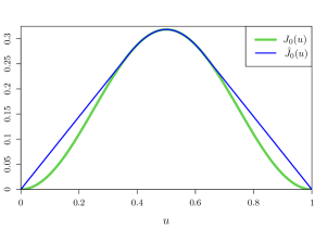
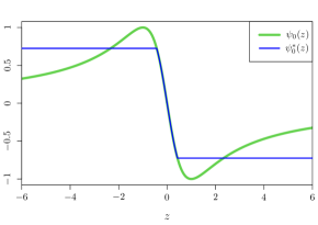
Figure 2: Left: The density quantile function $J_{0}$ and its least concave majorant $\hat{J}_{0}$ for a standard Cauchy density. Right: The corresponding score functions $\psi_{0}$ and $\psi_{0}^{*}$.

Theorem 2.

In the setting of Lemma 1, the following statements hold.

1. $\int_{\mathbb{R}}\psi_{0}^{*}\,dP_{0}=0$.

2. Let $i^{*}(p_{0}):=\int_{\mathbb{R}}(\psi_{0}^{*})^{2}\,dP_{0}$. Then $\inf_{\psi\in\Psi_{\downarrow}(p_{0})}D_{p_{0}}(\psi,\lambda)=-\lambda^{2}i^{*}(p_{0})$ for every $\lambda>0$.

3. Suppose that $i^{*}(p_{0})<\infty$. Then for each $\lambda>0$, the function $\lambda\psi_{0}^{*}$ is the unique minimiser of $D_{p_{0}}(\cdot\,,\lambda)$ over $\Psi_{\downarrow}(p_{0})$. Moreover, for every $\psi\in\Psi_{\downarrow}(p_{0})$ such that $\int_{\mathbb{R}}\psi^{2}\,dP_{0}>0$, we have

   $$V_{p_{0}}(\psi)\geq V_{p_{0}}(\psi_{0}^{*})=\frac{1}{i^{*}(p_{0})}\in(0,\infty),$$ (16)

   with equality if and only if $\psi=\lambda\psi_{0}^{*}$ for some $\lambda>0$.

4. Assume further that $p_{0}$ is absolutely continuous on $\mathbb{R}$ with derivative $p_{0}^{\prime}$ Lebesgue almost everywhere, corresponding score function $\psi_{0}:=p_{0}^{\prime}/p_{0}$ and Fisher information $i(p_{0}):=\int_{\mathbb{R}}\psi_{0}^{2}\,p_{0}$. Then

   $$\psi_{0}^{*}=\widehat{\mathcal{M}}_{\mathrm{R}}(\psi_{0}\circ F_{0}^{-1})\circ F_{0}$$ (17)

   and $0<i^{*}(p_{0})\leq i(p_{0})$, with equality if and only if $p_{0}$ is log-concave. In particular, if $i(p_{0})<\infty$, then the conclusions of (c) hold.

Some remarks are in order here. As mentioned in the introduction, Theorem 2(a) ensures the Fisher consistency of the regression $Z$-estimator $\hat{\beta}_{\psi_{0}^{*}}$ defined in (2). This reflects the fact that $\psi+c\in\Psi_{\downarrow}(p_{0})$ whenever $\psi\in\Psi_{\downarrow}(p_{0})$ and $c\in\mathbb{R}$; see (46) and the first-order stationarity condition (47). Moreover, (53) in the proof of Theorem 2(d) shows that

$$D_{p_{0}}(\psi,\lambda)=\int_{\mathbb{R}}(\psi-\lambda\psi_{0})^{2}\,dP_{0}-\int_{\mathbb{R}}(\lambda\psi_{0})^{2}\,dP_{0}=\|{\psi-\lambda\psi_{0}}\|_{L^{2}(P_{0})}^{2}-\lambda^{2}i(p_{0})$$

for all $\psi\in\Psi_{\downarrow}(p_{0})$, so if $i(p_{0})<\infty$, then Theorem 2(c) ensures that

$$\lambda\psi_{0}^{*}\in\operatorname*{argmin}_{\psi\in\Psi_{\downarrow}(p_{0})}D_{p_{0}}(\psi,\lambda)=\operatorname*{argmin}_{\psi\in\Psi_{\downarrow}(p_{0})}\|{\psi-\lambda\psi_{0}}\|_{L^{2}(P_{0})}^{2}.$$ (18)

Thus, in the terminology of Section 6.5, $\lambda\psi_{0}^{*}$ is a version of the $L^{2}(P_{0})$-antitonic projection of $\lambda\psi_{0}$ onto $\Psi_{\downarrow}(p_{0})$. Indeed, the explicit representation (17) of $\psi_{0}^{*}$ as a ‘monotonisation’ of $\psi_{0}$ (see the right panel of Figure 2) is consistent with that given in Proposition 43 for a general $L^{2}(P)$-antitonic projection, where $P$ is a univariate probability measure with a continuous distribution function.

When $i(p_{0})<\infty$, the inequality $i^{*}(p_{0})=\int_{\mathbb{R}}(\psi_{0}^{*})^{2}\,dP_{0}\leq\int_{\mathbb{R}}\psi_{0}^{2}\,dP_{0}=i(p_{0})$ in Theorem 2(d) follows from the fact that the $L^{2}(P_{0})$-antitonic projection onto the convex cone $\Psi_{\downarrow}(p_{0})$ is 1-Lipschitz with respect to $\|{{\cdot}}\|_{L^{2}(P_{0})}$; see (115) in Lemma 44. A statistical explanation of this information inequality arises from the fact that the $1/i(p_{0})$ is the infimum of the asymptotic variance functional $V_{p_{0}}(\psi)$ in (5) over all sufficiently regular $\psi\colon\mathbb{R}\to\mathbb{R}$; see Huber and Ronchetti, (2009, Theorem 4.2), which we restate as Proposition 36. On the other hand, by (16), $1/i^{*}(p_{0})$ is the minimum value of $V_{p_{0}}(\cdot)$ over the restricted class $\Psi_{\downarrow}(p_{0})$, so in view of our discussion in the introduction, it can be interpreted as an information lower bound for convex $M$-estimators. When $i^{*}(p_{0})<\infty$, the ratio

$$\mathrm{ARE}^{*}(p_{0}):=\frac{i^{*}(p_{0})}{i(p_{0})}$$

therefore quantifies the price we pay in statistical efficiency for insisting that our loss function be convex, and will be referred to as the antitonic relative efficiency. By Theorem 2(d), $\mathrm{ARE}^{*}(p_{0})\leq 1$ with equality if and only if $p_{0}$ is log-concave, so we can regard $1-\mathrm{ARE}^{*}(p_{0})$ as a measure of departure from log-concavity; see Section 2.2 below. Example 11 shows that $\mathrm{ARE}^{*}(p_{0})\approx 0.878$ when $p_{0}$ is the Cauchy density, whereas Example 25 in the appendix yields a density $p_{0}$ for which $\mathrm{ARE}^{*}(p_{0})=0$. More generally, in Lemma 7 below, we provide a simple lower bound on $\mathrm{ARE}^{*}(p_{0})$ that is reasonably tight for heavy-tailed densities $p_{0}$.

When $p_{0}$ is only uniformly continuous (and not absolutely continuous), the score function and Fisher information cannot be defined as above, but we nevertheless refer to $\psi_{0}^{*}$ and $i^{*}(p_{0})$ as the antitonic projected score function (see Lemma 5 below) and antitonic information (for location) respectively.

Remark 3.

Since $F_{0}$ is continuous, we have $(F_{0}\circ F_{0}^{-1})(u)=u$ for all $u\in(0,1)$. The concave function $\hat{J}_{0}$ is therefore absolutely continuous on $[0,1]$ with derivative $\hat{J}_{0}^{(\mathrm{R})}=\psi_{0}^{*}\circ F_{0}^{-1}$ Lebesgue almost everywhere (Rockafellar,, 1997, Corollary 24.2.1), so

$$i^{*}(p_{0})=\int_{\mathbb{R}}(\psi_{0}^{*})^{2}\,dP_{0}=\int_{0}^{1}(\psi_{0}^{*}\circ F_{0}^{-1})^{2}=\int_{0}^{1}\bigl{(}\hat{J}_{0}^{(\mathrm{R})}\bigr{)}^{2}.$$

In the setting of Theorem 2(d) above, a straightforward calculation (cf. (52) in the proof of Theorem 2) shows that the density quantile function $J_{0}=p_{0}\circ F_{0}^{-1}$ is absolutely continuous on $[0,1]$ with derivative $J_{0}^{\prime}=\psi_{0}\circ F_{0}^{-1}$ Lebesgue almost everywhere. Therefore, $\psi_{0}^{*}\circ F_{0}^{-1}=\hat{J}_{0}^{(\mathrm{R})}=\widehat{\mathcal{M}}_{\mathrm{R}}(\psi_{0}\circ F_{0}^{-1})$ almost everywhere and

$$i(p_{0})=\int_{\mathbb{R}}\psi_{0}^{2}\,dP_{0}=\int_{0}^{1}(\psi_{0}\circ F_{0}^{-1})^{2}=\int_{0}^{1}(J_{0}^{\prime})^{2}.$$

Finally in this subsection, we define the two-sided hazard function $h_{0}\colon\mathbb{R}\rightarrow[0,\infty)$ of $p_{0}$ by

$$h_{0}(z):=\frac{p_{0}(z)}{F_{0}(z)\wedge\bigl{(}1-F_{0}(z)\bigr{)}}=\begin{cases}p_{0}(z)/F_{0}(z)&\text{if }F_{0}(z)\leq 1/2\\ p_{0}(z)/\bigl{(}1-F_{0}(z)\bigr{)}&\text{if }F_{0}(z)>1/2,\end{cases}$$ (19)

where in accordance with our convention $0/0=0$, we have $h_{0}(z)=0$ whenever $F_{0}(z)\in\{0,1\}$. The following simple lemma provides a necessary and sufficient condition on the two-sided hazard function for $\psi_{0}^{*}$ to be appropriately bounded, which means that any negative antiderivative $\ell_{0}^{*}$ grows at most linearly, and therefore ensures robustness.

Lemma 4.

In the setting of Lemma 1, define $z_{\min}:=\inf(\operatorname{supp}p_{0})$ and $z_{\max}:=\sup(\operatorname{supp}p_{0})$. Then

1. $\lim_{z\to-\infty}\psi_{0}^{*}(z)<\infty$ if and only if $\limsup_{z\searrow z_{\min}}h_{0}(z)<\infty$, in which case $z_{\min}=-\infty$;

2. $\lim_{z\to\infty}\psi_{0}^{*}(z)>-\infty$ if and only if $\limsup_{z\nearrow z_{\max}}h_{0}(z)<\infty$, in which case $z_{\max}=\infty$.

Recall that a Laplace density has a constant two-sided hazard function, as well as a score function whose absolute value is constant. Roughly speaking, the conditions on $h_{0}$ in Lemma 4 are satisfied by densities whose tails are heavier than those of the Laplace density (Samworth and Johnson,, 2004), for which it is particularly attractive to have bounded projected score functions.

2.2 The log-concave Fisher divergence projection

Let $P_{0}$ and $P_{1}$ be Borel probability measures on $\mathbb{R}$ such that $P_{0}\ll P_{1}$. Write $\operatorname{supp}P_{0}$ for the support of $P_{0}$ (i.e. the smallest closed set $S$ satisfying $P_{0}(S)=1$), and $\operatorname{Int}(\operatorname{supp}P_{0})$ for its interior. Suppose that there exists a Radon–Nikodym derivative $dP_{0}/dP_{1}$ that is continuous on $\operatorname{Int}(\operatorname{supp}P_{0})$, and also strictly positive and differentiable on some subset $E\subseteq\operatorname{Int}(\operatorname{supp}P_{0})$ such that $P_{0}(E^{c})=0$. The Fisher divergence (also known as the Fisher information distance) from $P_{1}$ to $P_{0}$ is defined to be

$$I(P_{0},P_{1}):=\int_{E}\biggl{(}\Bigl{(}\log\frac{dP_{0}}{dP_{1}}\Bigr{)}^{\prime}\biggr{)}^{2}\,dP_{0}.$$ (20)

If $P_{0},P_{1}$ do not satisfy the assumptions above, then we define $I(P_{0},P_{1}):=\infty$. In the case where $P_{0},P_{1}$ have Lebesgue densities $p_{0},p_{1}$ respectively that are both locally absolutely continuous on $\mathbb{R}$, we have

$$I(p_{0},p_{1})\equiv I(P_{0},P_{1})=\begin{cases}\displaystyle\int_{\{p_{0}>0\}}\biggl{(}\Bigl{(}\log\frac{p_{0}}{p_{1}}\Bigr{)}^{\prime}\biggr{)}^{2}\,p_{0}=\int_{\mathbb{R}}(\psi_{0}-\psi_{1})^{2}\,dP_{0}\;&\text{if }\operatorname{supp}p_{0}\subseteq\operatorname{supp}p_{1}\\ \infty\;&\text{otherwise},\end{cases}$$

where we denote by $\psi_{j}:=(\log p_{j})^{\prime}\mathbbm{1}_{\{p_{j}>0\}}=p_{j}^{\prime}/p_{j}$ the corresponding score functions for $j\in\{0,1\}$. For further background on the Fisher divergence, see Johnson, (2004, Definition 1.13), Yang et al., (2019, Section 2) and references therein.

The following lemma establishes the connection between the projected score function and the Fisher divergence.

Lemma 5.

In the setting of Lemma 1, there is a unique continuous log-concave density $p_{0}^{*}$ on $\mathbb{R}$ such that $\operatorname{supp}p_{0}^{*}=\mathcal{S}_{0}$ and $\log p_{0}^{*}$ has right derivative $\psi_{0}^{*}$ on $\mathcal{S}_{0}$. In particular, $\psi_{0}^{*}=(\log p_{0}^{*})^{\prime}$ Lebesgue almost everywhere on $\mathcal{S}_{0}$. Furthermore, if $p_{0}$ is itself log-concave, then $p_{0}^{*}=p_{0}$.

When $p_{0}$ is absolutely continuous, (18) indicates that the log-concave density $p_{0}^{*}$ (with score function $\psi_{0}^{*}\mathbbm{1}_{\mathcal{S}_{0}}$) in Lemma 5 minimises $I(p_{0},p)$ over the class $\mathcal{P}_{\mathrm{LC}}$ of all univariate log-concave densities $p$. Moreover, $p_{0}^{*}=p_{0}$ if and only if $p_{0}$ is log-concave. Even when $p_{0}$ is only uniformly continuous, we refer to $p_{0}^{*}$ as the log-concave Fisher divergence projection of $p_{0}$. In contrast, the log-concave maximum likelihood projection $p_{0}^{\mathrm{ML}}$ of the distribution $P_{0}$ (Dümbgen et al.,, 2011; Barber and Samworth,, 2021) can be interpreted as a minimiser of Kullback–Leibler divergence rather than Fisher divergence over the class of upper semi-continuous log-concave densities. By Dümbgen et al., (2011, Theorem 2.2), $p_{0}^{\mathrm{ML}}$ exists and is unique if and only if $P_{0}$ is non-degenerate and has a finite mean (but not necessarily a Lebesgue density). On the other hand, moment conditions are not required for $p_{0}^{*}$ to exist and be unique, but $p_{0}^{*}$ is only defined in Lemma 5 when $P_{0}$ has a uniformly continuous density on $\mathbb{R}$. As we will discuss in Section 2.4, the non-existence of the Fisher divergence projection for discrete measures $P_{0}$ has consequences for our statistical methodology.

When $p_{0}$ is not log-concave, $p_{0}^{\mathrm{ML}}$ usually does not coincide with $p_{0}^{*}$ even when both exist, and moreover the associated regression $M$-estimators

$$\hat{\beta}_{\psi_{0}^{\mathrm{ML}}}\in\operatorname*{argmax}_{\beta\in\mathbb{R}^{d}}\sum_{i=1}^{n}\log p_{0}^{\mathrm{ML}}(Y_{i}-X_{i}^{\top}\beta)\quad\text{and}\quad\hat{\beta}_{\psi_{0}^{*}}\in\operatorname*{argmax}_{\beta\in\mathbb{R}^{d}}\sum_{i=1}^{n}\log p_{0}^{*}(Y_{i}-X_{i}^{\top}\beta)$$ (21)

are generally different; see Examples 12 and 26 below. In fact, the following result shows that there exist error distributions $P_{0}$ for which the asymptotic covariance of $\hat{\beta}_{\psi_{0}^{\mathrm{ML}}}$ is arbitrarily large compared with that of the optimal convex $M$-estimator $\hat{\beta}_{\psi_{0}^{*}}$, even when the latter is close to being asymptotically efficient in the sense of (4).

Proposition 6.

For every $\epsilon\in(0,1)$, there exists a distribution $P_{0}$ with a finite mean and an absolutely continuous density $p_{0}$ such that $i(p_{0})<\infty$, and the log-concave maximum likelihood projection $q_{0}\equiv p_{0}^{\mathrm{ML}}$ has corresponding score function $\psi_{0}^{\mathrm{ML}}:=q_{0}^{(\mathrm{R})}/q_{0}\in\Psi_{\downarrow}(p_{0})$ satisfying

$$\frac{V_{p_{0}}(\psi_{0}^{*})}{V_{p_{0}}(\psi_{0}^{\mathrm{ML}})}\leq\epsilon\quad\text{and}\quad\mathrm{ARE}^{*}(p_{0})\geq 1-\epsilon.$$ (22)

Our next result provides a simple lower bound on the antitonic information.

Lemma 7.

Suppose that $p_{0}$ is an absolutely continuous density on $\mathbb{R}$ with $i(p_{0})<\infty$. Then $p_{0}$ is bounded with $i^{*}(p_{0})\geq 4\|{p_{0}}\|_{\infty}^{2}$, so

$$\mathrm{ARE}^{*}(p_{0})\geq\frac{4\|{p_{0}}\|_{\infty}^{2}}{i(p_{0})},$$

with equality if and only if $p_{0}^{*}$ is a Laplace density, i.e. there exist $\mu\in\mathbb{R}$ and $\sigma>0$ such that $p_{0}^{*}(z)=(2\sigma)^{-1}\exp(-|z-\mu|/\sigma)$ for all $z\in\mathbb{R}$.

Remark 8.

A reassuring property of the antitonic projection is its affine equivariance: if $p_{0}$ is a uniformly continuous density, then for $a>0$ and $b\in\mathbb{R}$, the density $z\mapsto ap_{0}(az+b)=:p_{a,b}(z)$ has antitonic projected score function and log-concave Fisher divergence projection given by

$$\psi_{a,b}^{*}(z):=a\psi_{0}^{*}(az+b)\quad\text{and}\quad p_{a,b}^{*}(z):=ap_{0}^{*}(az+b)$$

respectively for $z\in\mathbb{R}$. It follows that $1/V_{p_{a,b}}(\psi_{a,b}^{*})=i^{*}(p_{a,b})=\int_{-\infty}^{\infty}(\psi_{a,b}^{*})^{2}\,p_{a,b}=a^{2}i^{*}(p_{0})$, so because $\|{p_{a,b}}\|_{\infty}=a\|{p_{0}}\|_{\infty}$, both the antitonic relative efficiency and the lower bound in Lemma 7 are affine invariant in the sense that they remain unchanged if we replace $p_{0}$ with $p_{a,b}$.

Similarly, if $P_{0}$ has a finite mean, then by the affine equivariance of the log-concave maximum likelihood projection (Dümbgen et al.,, 2011, Remark 2.4), $p_{a,b}^{\mathrm{ML}}(z)=ap_{0}^{\mathrm{ML}}(az+b)$ and hence $\psi_{a,b}^{\mathrm{ML}}=a\psi_{0}^{\mathrm{ML}}(az+b)$ for $z\in\mathbb{R}$. Thus, $V_{p_{a,b}}(\psi_{a,b}^{\mathrm{ML}})=V_{p_{0}}(\psi_{0}^{\mathrm{ML}})/a^{2}$, so the first ratio in (22) is also affine invariant. Consequently, for any $C\in(0,\infty)$, $\mu\in\mathbb{R}$ and $\epsilon\in(0,1)$, there exists a density $p_{0}$ satisfying (22) with $i(p_{0})=C$ and $\int_{\mathbb{R}}zp_{0}(z)\,dz=\mu$.

The final result in this subsection relates properties of densities and their log-concave Fisher divergence projections.

Proposition 9.

For a uniformly continuous density $p_{0}\colon\mathbb{R}\to\mathbb{R}$, the log-concave Fisher divergence projection $p_{0}^{*}$ and its corresponding distribution function $F_{0}^{*}\colon[-\infty,\infty]\to\mathbb{R}$ have the following properties.

1. Denote by $\mathcal{T}$ the set of $z\in\mathcal{S}_{0}$ such that $\psi_{0}^{*}$ is non-constant on every open interval containing $z$. For $z\in\mathcal{T}$, we have

   $$\frac{p_{0}^{*}(z)}{F_{0}^{*}(z)}\leq\frac{p_{0}(z)}{F_{0}(z)}\quad\text{and}\quad\frac{p_{0}^{*}(z)}{1-F_{0}^{*}(z)}\leq\frac{p_{0}(z)}{1-F_{0}(z)},$$ (23)

   whence $p_{0}^{*}(z)\leq p_{0}(z)$.

2. $\|{p_{0}^{*}}\|_{\infty}\leq\|{p_{0}}\|_{\infty}$ and $i(p_{0}^{*})=-\int_{\mathbb{R}}p_{0}^{*}\,d\psi_{0}^{*}\leq-\int_{\mathbb{R}}p_{0}\,d\psi_{0}^{*}=i^{*}(p_{0})$.

We can define the two-sided hazard function $h_{0}^{*}$ of the log-concave Fisher divergence projection $p_{0}^{*}$ analogously to $h_{0}$ in (19). Since $p_{0}^{*}$ is log-concave, its density quantile function $J_{0}^{*}:=p_{0}^{*}\circ(F_{0}^{*})^{-1}$ has decreasing right derivative $(J_{0}^{*})^{(\mathrm{R})}=\psi_{0}^{*}\circ(F_{0}^{*})^{-1}$ by (the proof of) Lemma 5, so $J_{0}^{*}$ is concave on $[0,1]$. Thus,

$$0=J_{0}^{*}(0)\leq J_{0}^{*}(u)-u(J_{0}^{*})^{(\mathrm{R})}(u)\quad\text{and}\quad 0=J_{0}^{*}(1)\leq J_{0}^{*}(u)+(1-u)(J_{0}^{*})^{(\mathrm{R})}(u)$$

for all $u\in[0,1]$, so for $z\in\mathcal{T}$, Lemma 1 and (23) in Proposition 9(a) imply that

$$|\psi_{0}^{*}(z)|=\bigl{|}(J_{0}^{*})^{(\mathrm{R})}\bigl{(}F_{0}^{*}(z)\bigr{)}\bigr{|}\leq\frac{J_{0}^{*}\bigl{(}F_{0}^{*}(z)\bigr{)}}{F_{0}^{*}(z)\wedge\bigl{(}1-F_{0}^{*}(z)\bigr{)}} =\frac{p_{0}^{*}(z)}{F_{0}^{*}(z)\wedge\bigl{(}1-F_{0}^{*}(z)\bigr{)}}=h_{0}^{*}(z)$$

$$\leq\frac{p_{0}(z)}{F_{0}(z)\wedge\bigl{(}1-F_{0}(z)\bigr{)}}=h_{0}(z).$$

Proposition 9(b) provides inequalities on the supremum norm and antitonic information of the log-concave Fisher divergence projection. In particular, the Fisher information of the projected density is at most the antitonic information of the original density.

2.3 Examples

Example 10.

Let $p_{0}$ be the $\mathrm{Beta}(a,b)$ density given by $p_{0}(z)=z^{a-1}(1-z)^{b-1}\mathbbm{1}_{\{z\in(0,1)\}}/\mathrm{B}(a,b)$ for $a,b>1$, where $\mathrm{B}$ denotes the beta function. Then $p_{0}$ is uniformly continuous and log-concave on $\mathbb{R}$, so

$$\psi_{0}^{*}(z)=\psi_{0}(z)=(\log p_{0})^{\prime}(z)=\frac{a-1}{z}-\frac{b-1}{1-z}$$

for all $z\in(0,1)$, while $\psi_{0}^{*}(z)=\infty$ for $z\leq 0$ and $\psi_{0}^{*}(z)=-\infty$ for $z\geq 1$. We have $i^{*}(p_{0})=i(p_{0})=\int_{0}^{1}\psi_{0}^{2}\,p_{0}<\infty$ if and only if $a,b>2$, in which case the conclusions of Theorem 2(c, d) hold.

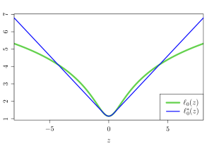
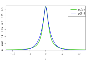
Figure 3: Left: The negative log-density $\ell_{0}=-\log p_{0}$ and the optimal convex loss function $\ell_{0}^{*}=-\log p_{0}^{*}$ when $p_{0}$ is the standard Cauchy density. Right: The corresponding densities $p_{0}$ and $p_{0}^{*}$.

Example 11.

Let $p_{0}$ be the standard Cauchy density given by $p_{0}(z)=1/\bigl{(}\pi(1+z^{2})\bigr{)}$ for $z\in\mathbb{R}$. Then $p_{0}$ is absolutely continuous on $\mathbb{R}$ with $i(p_{0})=\int_{\mathbb{R}}(p_{0}^{\prime})^{2}/p_{0}=1/2$ and $\lim_{z\to\pm\infty}h_{0}(z)=0$. We will derive an explicit expression for $\psi_{0}^{*}$, which is necessarily bounded by Lemma 4. In contrast to the previous example, $p_{0}$ is not log-concave, so $\psi_{0}^{*}$ does not coincide with $\psi_{0}=p_{0}^{\prime}/p_{0}\colon z\mapsto-2z/(1+z^{2})$. Indeed,

$$F_{0}(z) =\frac{1}{2}+\frac{\arctan(z)}{\pi}\;\;\text{for }z\in\mathbb{R},\qquad F_{0}^{-1}(u)=\tan\biggl{(}\pi\Bigl{(}u-\frac{1}{2}\Bigr{)}\biggr{)}=-\cot(\pi u)\;\;\text{for }u\in(0,1),$$

$$J_{0}(u) =\frac{1}{\pi\bigl{(}1+\cot^{2}(\pi u)\bigr{)}}=\frac{\sin^{2}(\pi u)}{\pi}=\frac{1-\cos(2\pi u)}{2\pi}\;\;\text{for }u\in[0,1].$$

Let $\zeta_{0}\approx 2.33$ be the unique $\zeta\in(0,\pi)$ satisfying $\zeta=\tan(\zeta/2)$, and define $u_{0}:=\zeta_{0}/(2\pi)\in(0,1/2)$. Then we can verify that $\hat{J}_{0}$ is linear on $[0,u_{0}]$ and on $[1-u_{0},1]$, with $\hat{J}_{0}(u)=J_{0}(u)$ for $u\in[u_{0},1-u_{0}]\cup\{0,1\}$; see the left panel of Figure 2. It follows that

$$\hat{J}_{0}^{(\mathrm{R})}(u) =\begin{cases}\,\sin\zeta_{0}&\text{for }u\in[0,u_{0}]\\ \,\sin(2\pi u)&\text{for }u\in[u_{0},1-u_{0}]\\ \,-\sin\zeta_{0}&\text{for }u\in[1-u_{0},1];\end{cases}$$

$$\psi_{0}^{*}(z)=\hat{J}_{0}^{(\mathrm{R})}\bigl{(}F_{0}(z)\bigr{)} =\begin{cases}\,\sin\zeta_{0}=-2z_{0}/(1+z_{0}^{2})&\text{for }z\in(-\infty,-z_{0}]\\ \,-\sin(2\arctan z)=-2z/(1+z^{2})=\psi_{0}(z)&\text{for }z\in[-z_{0},z_{0}]\\ \,-\sin\zeta_{0}&\text{for }z\in[z_{0},\infty),\end{cases}$$

where $z_{0}:=\cot(\pi u_{0})=\cot(\zeta_{0}/2)\approx 0.43\in(0,1)$ satisfies $z_{0}\arctan(1/z_{0})=1/2$. Thus, $\psi_{0}^{*}(z)=\psi_{0}\bigl{(}(z\wedge z_{0})\vee(-z_{0})\bigr{)}$ for $z\in\mathbb{R}$; see the right panel of Figure 2. An antiderivative $\phi_{0}^{*}$ of $\psi_{0}^{*}$ is given by

$$\phi_{0}^{*}(z):=\int_{0}^{z}\psi_{0}^{*}-\log\pi=\begin{cases}\,-\log\bigl{(}\pi(1+z^{2})\bigr{)}&\text{for }z\in[-z_{0},z_{0}]\\ \,-(|z|-z_{0})\sin\zeta_{0}-\log\bigl{(}\pi(1+z_{0}^{2})\bigr{)}&\text{for }z\in\mathbb{R}\setminus[-z_{0},z_{0}].\end{cases}$$

As illustrated in the left panel of Figure 3, $\ell_{0}^{*}:=-\phi_{0}^{*}$ is a symmetric convex function that is approximately quadratic on $[-z_{0},z_{0}]$ and linear outside this interval, so in this respect, it resembles the Huber loss function (7). This is significant as far as $M$-estimation is concerned, since Huber-like loss functions are designed precisely to be robust to outliers, such as those that arise in regression problems with heavy-tailed Cauchy errors. As discussed in the introduction, $\ell_{0}^{*}$ is optimal in the sense that the resulting regression $M$-estimator $\hat{\beta}_{\psi_{0}^{*}}\in\operatorname*{argmin}_{\beta\in\mathbb{R}^{d}}\sum_{i=1}^{n}\ell_{0}^{*}(Y_{i}-X_{i}^{\top}\beta)$ has minimal asymptotic covariance (3) among all convex $M$-estimators. By direct computation,

$$\frac{1}{V_{p_{0}}(\psi_{0}^{*})}=i^{*}(p_{0})=\frac{1}{2}-\frac{2\zeta_{0}\cos(2\zeta_{0})-\sin(2\zeta_{0})}{4\pi}\approx 0.439,\;\;\text{so}\;\;\mathrm{ARE}^{*}(p_{0})=\frac{i^{*}(p_{0})}{i(p_{0})}\approx 0.878$$

in this case, meaning that the restriction to convex loss functions results in only a small loss of efficiency relative to the maximum likelihood estimator. This may well be outweighed by the increased computational convenience of optimising a convex empirical risk function as opposed to a Cauchy likelihood function, which typically has several local extrema; see van der Vaart, (1998, Example 5.50) for a discussion of the difficulties involved. Lemma 7 yields the bound $\mathrm{ARE}^{*}(p_{0})\geq 8\|{p_{0}}\|_{\infty}^{2}=8/\pi^{2}\approx 0.811$.

Figure 4: Plot of the asymptotic relative efficiency $r(K)$ of the Huber $M$-estimator $\hat{\beta}_{\psi_{K}}$ compared with the optimal convex $M$-estimator.

For $K>0$, the Huber regression $M$-estimator $\hat{\beta}_{\psi_{K}}\in\operatorname*{argmin}_{\beta\in\mathbb{R}^{d}}\sum_{i=1}^{n}\ell_{K}(Y_{i}-X_{i}^{\top}\beta)$ defined with respect to (7) has asymptotic relative efficiency

$$r(K):=\frac{V_{p_{0}}(\psi_{0}^{*})}{V_{p_{0}}(\psi_{K})}=\frac{\pi\bigl{(}\pi K^{2}+2K-2(1+K^{2})\arctan K\bigr{)}}{4i^{*}(p_{0})\arctan^{2}K}$$

compared with the optimal convex $M$-estimator $\hat{\beta}_{\psi_{0}^{*}}$; see Figure 4. The maximum value $\sup_{K>0}r(K)\approx 0.9998$ is attained at $K^{*}\approx 0.394$. Moreover,

$$\lim_{K\to 0}r(K)=\frac{4}{\pi^{2}i^{*}(p_{0})}\approx 0.922$$

is the asymptotic relative efficiency $V_{p_{0}}(\psi_{0}^{*})/V_{p_{0}}(\psi)$ of the least absolute deviation (LAD) estimator $\hat{\beta}_{\psi}\in\operatorname*{argmin}_{\beta\in\mathbb{R}^{d}}\sum_{i=1}^{n}|Y_{i}-X_{i}^{\top}\beta|$, for which $\psi(\cdot):=-\operatorname{sgn}(\cdot)$ and $V_{p_{0}}(\psi)=1/\bigl{(}4p_{0}(0)^{2}\bigr{)}=\pi^{2}/4$. On the other hand, the Huber loss $\ell_{K}$ in (7) converges pointwise to the squared error loss as $K\to\infty$, so $\lim_{K\to\infty}V_{p_{0}}(\psi_{K})=\int_{\mathbb{R}}z^{2}\,p_{0}(z)\,dz=\infty$ and hence $\lim_{K\to\infty}r(K)=0$. We recall the difficulties of choosing $K$, and its connection to the choice of scale, from the discussion in the introduction.

The Cauchy density $p_{0}$ and its log-concave Fisher divergence projection $p_{0}^{*}:=e^{\phi_{0}^{*}}$ are plotted in the right panel of Figure 3. Since $p_{0}=p_{0}^{*}$ on $[-z_{0},z_{0}]$ and $\psi_{0}^{*}$ is constant on $\mathbb{R}\setminus[-z_{0},z_{0}]$, it turns out that $i^{*}(p_{0})=-\int_{\mathbb{R}}p_{0}\,d\psi_{0}^{*}=-\int_{\mathbb{R}}p_{0}^{*}\,d\psi_{0}^{*}=i(p_{0}^{*})$, so both inequalities in Proposition 9(b) are in fact equalities in this example.

In Example 26 in the appendix, we take $P_{0}$ to be a scaled $t_{2}$ distribution, which has a finite first moment (unlike the Cauchy distribution in Example 11), and verify that $\hat{\beta}_{\psi_{0}^{\mathrm{ML}}}$ and $\hat{\beta}_{\psi_{0}^{*}}$ in (21) are different convex $M$-estimators. Example 27 features a symmetrised Pareto density with polynomially decaying tails, where the optimal convex loss function $\ell_{0}^{*}$ is a scale transformation of the robust absolute error loss $z\mapsto|z|$.

Moving on from heavy-tailed distributions, we now consider a density $p_{0}$ that fails to be log-concave because it is not unimodal.

Example 12.

For $\rho\in(0,1)$ and $\mu>0$, let $p_{0}$ be the two-component Laplace mixture density given by

$$p_{0}(z)=\frac{1-\rho}{2}e^{-|z+\mu|}+\frac{\rho}{2}e^{-|z-\mu|}$$

for $z\in\mathbb{R}$. The corresponding score function $\psi_{0}=(\log p_{0})^{\prime}=p_{0}^{\prime}/p_{0}$ satisfies

$$\psi_{0}(z)=\begin{cases}1\;\;&\text{for }z<-\mu\\ \dfrac{\rho e^{z}-(1-\rho)e^{-z}}{\rho e^{z}+(1-\rho)e^{-z}}\;\;&\text{for }z\in(-\mu,\mu)\\ -1\;\;&\text{for }z>\mu,\end{cases}$$

so $\psi_{0}$ is strictly increasing on $(-\mu,\mu)$ and constant on both $(-\infty,\mu)$ and $(\mu,\infty)$. Since $J_{0}^{\prime}=\psi_{0}\circ F_{0}^{-1}$ on $(0,1)\setminus\{F_{0}(-\mu),F_{0}(\mu)\}$, it follows that $J_{0}$ is convex on $[F_{0}(-\mu),F_{0}(\mu)]$ while being linear on both $[0,F_{0}(-\mu)]$ and $[F_{0}(\mu),1]$. Therefore, $\hat{J}_{0}=J_{0}$ on $[0,F_{0}(-\mu)]\cup[F_{0}(\mu),1]$ and $\hat{J}_{0}$ is linear on $[F_{0}(-\mu),F_{0}(\mu)]$ with $J_{0}\bigl{(}F_{0}(\pm\mu)\bigr{)}=p_{0}(\pm\mu)$, so

$$\psi_{0}^{*}(z)=\hat{J}_{0}^{(\mathrm{R})}\bigl{(}F_{0}(z)\bigr{)}=\begin{cases}1\;\;&\text{for }z<-\mu\\ \dfrac{p_{0}(\mu)-p_{0}(-\mu)}{F_{0}(\mu)-F_{0}(-\mu)}=2\rho-1\;\;&\text{for }z\in[-\mu,\mu)\\ -1\;\;&\text{for }z\geq\mu,\end{cases}$$

and hence

$$p_{0}^{*}(z)=\begin{cases}Ce^{z+\mu}\;\;&\text{for }z\leq-\mu\\ Ce^{(2\rho-1)(z+\mu)}\;\;&\text{for }z\in[-\mu,\mu]\\ Ce^{(2\rho-1)2\mu}\cdot e^{-(z-\mu)}\;\;&\text{for }z\geq\mu,\end{cases}\qquad\text{where }C:=\frac{1}{1+e^{(2\rho-1)2\mu}+\int_{0}^{2\mu}e^{(2\rho-1)z}\,dz}.$$

By direct calculation, $p_{0}^{*}(-\mu)=C<p_{0}(-\mu)$ and $p_{0}^{*}(\mu)=Ce^{(2\rho-1)2\mu}<p_{0}(\mu)$, so $\|{p_{0}^{*}}\|_{\infty}=p_{0}^{*}(-\mu)\vee p_{0}^{*}(\mu)<p_{0}(-\mu)\vee p_{0}(\mu)=\|{p_{0}}\|_{\infty}$ and

$$i^{*}(p_{0})=-\int_{\mathbb{R}}p_{0}\,d\psi_{0}^{*}=2(1-\rho)\cdot p_{0}(-\mu)+2(1+\rho)\cdot p_{0}(\mu)>2(1-\rho)\cdot p_{0}^{*}(-\mu)+2(1+\rho)\cdot p_{0}^{*}(\mu)=i(p_{0}^{*}).$$

We mention that Proposition 6 can be proved by slightly modifying the construction of $p_{0}$ in Example 12.

2.4 Estimation of the projected score function

Theorem 2 motivates a general-purpose nonparametric procedure to estimate the antitonic projected score function $\psi_{0}^{*}$ based on a sample $\varepsilon_{1},\dotsc,\varepsilon_{n}\overset{\mathrm{iid}}{\sim}p_{0}$. We will first explain why a naive approach fails before describing our methodology. For a locally absolutely continuous function $\psi\colon\mathbb{R}\to\mathbb{R}$ with derivative $\psi^{\prime}$, the empirical analogue of $D_{p_{0}}(\psi)=\mathbb{E}\bigl{(}\psi^{2}(\varepsilon_{1})+2\psi^{\prime}(\varepsilon_{1})\bigr{)}$ in (14) is

$$\hat{D}_{n}(\psi)\equiv\hat{D}_{n}(\psi;\varepsilon_{1},\dotsc,\varepsilon_{n}):=\frac{1}{n}\sum_{i=1}^{n}\{\psi^{2}(\varepsilon_{i})+2\psi^{\prime}(\varepsilon_{i})\}.$$ (24)

Recall from the introduction that score matching estimates the score function $\psi_{0}=p_{0}^{\prime}/p_{0}$ (associated with a locally absolutely continuous $p_{0}$) by an empirical risk minimiser $\hat{\psi}_{n}\in\operatorname*{argmin}_{\psi\in\Psi}\hat{D}_{n}(\psi)$ over an appropriate class of functions $\Psi$.

However, to obtain a monotone score estimate, we cannot minimise $\psi\mapsto\hat{D}_{n}(\psi)$ directly over the class $\Psi_{\downarrow}^{\mathrm{ac}}$ of all decreasing, locally absolutely continuous $\psi\colon\mathbb{R}\to\mathbb{R}$. Indeed, $\inf_{\psi\in\Psi_{\downarrow}^{\mathrm{ac}}}\hat{D}_{n}(\psi)=-\infty$, as can be seen by constructing differentiable approximations to a decreasing step function whose jumps are at the data points $\varepsilon_{1},\dotsc,\varepsilon_{n}$. To circumvent this issue, we instead propose the following estimation strategy.

Antitonic projected score estimation: Consider smoothing the empirical distribution of $\varepsilon_{1},\dotsc,\varepsilon_{n}$, for example by convolving it with an absolutely continuous kernel $K\colon\mathbb{R}\to\mathbb{R}$ to obtain a kernel density estimator $z\mapsto\tilde{p}_{n}(z):=n^{-1}\sum_{i=1}^{n}K_{h}(z-\varepsilon_{i})$, where $h>0$ is a suitable bandwidth and $K_{h}(\cdot):=h^{-1}K(\cdot/h)$. We can then define the smoothed empirical score matching objective

$$\tilde{D}_{n}(\psi):=D_{\tilde{p}_{n}}(\psi)=\int_{-\infty}^{\infty}\psi^{2}\,\tilde{p}_{n}+2\int_{\mathcal{S}_{0}}\tilde{p}_{n}\,d\psi$$

for $\psi\in\Psi_{\downarrow}(\tilde{p}_{n})$, which approximates the population expectation in the definition of $D_{p_{0}}(\psi)$. Then by Theorem 2,

$$\hat{\psi}_{n}:=\hat{J}_{n}^{(\mathrm{R})}\circ\tilde{F}_{n}\in\operatorname*{argmin}_{\psi\in\Psi_{\downarrow}(\tilde{p}_{n})}\tilde{D}_{n}(\psi),$$ (25)

where $\tilde{F}_{n}$ denotes the distribution function corresponding to $\tilde{p}_{n}$, and $J_{n}:=\tilde{p}_{n}\circ\tilde{F}_{n}^{-1}$. This is reminiscent of maximum smoothed likelihood estimation of a density or distribution function (e.g. Eggermont and LaRiccia,, 2000; Groeneboom and Jongbloed,, 2014, Sections 8.2 and 8.5). By evaluating the antiderivative of $J_{n}$ on a suitably fine grid, we may obtain a piecewise affine approximation to $\hat{J}_{n}$ (and hence a piecewise constant approximation to its derivative) using PAVA, whose space and time complexities scale linearly with the size of the grid (Samworth and Shah,, 2024, Section 10.3.1).

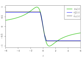
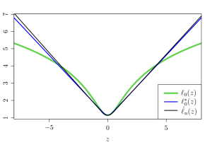
Figure 5: Kernel-based estimates of the projected score function and optimal convex loss function based on a sample of size $n=2000$ from the Cauchy distribution.

More generally, we can use $\varepsilon_{1},\dotsc,\varepsilon_{n}$ to construct a generic (not necessarily monotone) score estimator $\tilde{\psi}_{n}$ and an estimate $\hat{F}_{n}$ of the distribution function $F_{0}$ corresponding to the density $p_{0}$. By analogy with the explicit representation (17) of $\psi_{0}^{*}$, we then define the decreasing score estimate

$$\hat{\psi}_{n}:=\widehat{\mathcal{M}}_{\mathrm{R}}(\tilde{\psi}_{n}\circ\hat{F}_{n}^{-1})\circ\hat{F}_{n}.$$ (26)

As explained above, (an approximation to) $\hat{\psi}_{n}$ can be computed efficiently using isotonic regression algorithms. In particular, if $\hat{F}_{n}$ is taken to be the empirical distribution function of $\varepsilon_{1},\dotsc,\varepsilon_{n}$, then by Proposition 43, $\hat{\psi}_{n}^{\mathrm{L}}:=\widehat{\mathcal{M}}_{\mathrm{L}}(\tilde{\psi}_{n}\circ\hat{F}_{n}^{-1})\circ\hat{F}_{n}$ is an antitonic least squares estimator based on $\bigl{\{}\bigl{(}\varepsilon_{i},\tilde{\psi}_{n}(\varepsilon_{i})\bigr{)}:i\in[n]\bigr{\}}$. Our decreasing score estimate can be taken to be either $\hat{\psi}_{n}^{\mathrm{L}}$ or the closely related $\hat{\psi}_{n}$: for every $z\in\mathbb{R}$, we have $\hat{\psi}_{n}(z)=\hat{\psi}_{n}^{\mathrm{L}}\bigl{(}\varepsilon(z)\bigr{)}$, where $\varepsilon(z)$ is the smallest element of $\{\varepsilon_{1},\dotsc,\varepsilon_{n}\}$ that is either strictly greater than $z$ or equal to $\max_{i\in[n]}\varepsilon_{i}$.

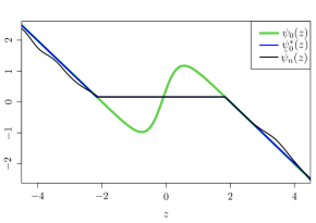
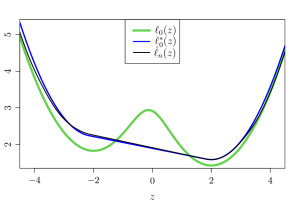
Figure 6: Kernel-based estimates of the projected score function and optimal convex loss function based on a sample of size $n=10^{4}$ from the Gaussian mixture distribution $0.4N(-2,1)+0.6N(2,1)$.

The transformation (26) may be applied to any appropriate initial score estimator $\tilde{\psi}_{n}$. Since a misspecified parametric method may introduce significant error at the outset, we seek a nonparametric estimator. For instance, we may take $\tilde{\psi}_{n}$ to be a ratio of kernel density estimates of $p_{0}^{\prime}$ and $p_{0}$, which may be truncated for theoretical and practical convenience to avoid instability in low-density regions; see (31) in Section 3.1. Observe that (25) is a special case of (26) with $\tilde{\psi}_{n}=\tilde{p}_{n}^{\prime}/\tilde{p}_{n}$ and $\hat{F}_{n}=\tilde{F}_{n}$.

3 Semiparametric $M$-estimation via antitonic score matching

Suppose that we observe independent and identically distributed pairs $(X_{1},Y_{1}),\dotsc,(X_{n},Y_{n})$ satisfying

$$Y_{i}=X_{i}^{\top}\beta_{0}+\varepsilon_{i}\quad\text{for }i\in[n],$$ (27)

where $X_{1},\dotsc,X_{n}$ are $\mathbb{R}^{d}$-valued covariates that are independent of errors $\varepsilon_{1},\dotsc,\varepsilon_{n}$ with an unknown absolutely continuous (Lebesgue) density $p_{0}$ on $\mathbb{R}$. We do not necessarily insist that $\mathbb{E}(\varepsilon_{1})=0$, because we also have in mind settings where we might want to assume that a quantile (e.g. the median) of $\varepsilon_{1}$ is zero. In fact, we do not even assume that $\mathbb{E}(\varepsilon_{1})$ is well-defined, which allows us to consider Cauchy errors, for instance, as a running example. A price to pay for this generality is that if an intercept term is present in (27), i.e. $X_{id}=1$ for each $i\in[n]$, then the corresponding component $\beta_{0d}$ of $\beta_{0}$ is unidentifiable. On a related point, a necessary condition for $\beta_{0}$ to be identifiable is that $\mathbb{E}(X_{1}X_{1}^{\top})$ is positive definite. Indeed, if this matrix is singular, then there exists $v\in\mathbb{R}^{d}\setminus\{0\}$ such that $X_{i}^{\top}v=0$ for all $i$ almost surely; in that case, the joint distribution of our observed data is unchanged if we replace $\beta_{0}$ with $\beta_{0}+v$. This identifiability issue is discussed in greater detail following the statement of Proposition 13.

For $\beta\in\mathbb{R}^{d}$, define $q_{\beta}\colon\mathbb{R}\to\mathbb{R}$ by

$$q_{\beta}(z):=\mathbb{E}p_{0}\bigl{(}z-X_{1}^{\top}(\beta_{0}-\beta)\bigr{)},$$

so that $q_{\beta}$ is the density of $Y_{1}-X_{1}^{\top}\beta=\varepsilon_{1}+X_{1}^{\top}(\beta_{0}-\beta)$.

Our approach to estimating $\beta_{0}$ with data-driven convex loss functions is motivated by the following population-level optimisation problem. We seek to minimise the augmented score matching objective

$$Q(\beta,\psi):=D_{q_{\beta}}(\psi)=\mathbb{E}\biggl{(}\int_{-\infty}^{\infty}\psi^{2}\bigl{(}z+X_{1}^{\top}(\beta_{0}-\beta)\bigr{)}\,p_{0}(z)\,dz+2\int_{\mathbb{R}}p_{0}\bigl{(}z-X_{1}^{\top}(\beta_{0}-\beta)\bigr{)}\,d\psi(z)\biggr{)}$$ (28)

jointly over $\beta\in\mathbb{R}^{d}$ and $\psi\in\Psi_{\downarrow}(q_{\beta})$ satisfying

$$\mathbb{E}\bigl{(}X_{1}\psi(Y_{1}-X_{1}^{\top}\beta)\bigr{)}=0.$$ (29)

Recall from (14) that if $\psi\in\Psi_{\downarrow}(q_{\beta})$ is locally absolutely continuous on $\mathbb{R}$, then

$$Q(\beta,\psi)=\mathbb{E}\psi^{2}(Y_{1}-X_{1}^{\top}\beta)+2\mathbb{E}\psi^{\prime}(Y_{1}-X_{1}^{\top}\beta).$$

The constraint (29) is the population analogue of the estimating equations (2) based on $\psi$. It forces $\beta$ to be a minimiser of the convex population risk function $b\mapsto\mathbb{E}\ell(Y_{1}-X_{1}^{\top}b)=:L_{\psi}(b)$ over $\mathcal{D}_{\psi}$, where $\ell$ is any negative antiderivative of $\psi$, and $\mathcal{D}_{\psi}$ is the convex set of $b\in\mathbb{R}^{d}$ such that $L_{\psi}(b)$ is well-defined in $[-\infty,\infty]$..

The following proposition characterises the global joint minimiser of our constrained score matching optimisation problem. For $j\in[d]$, write $\mathsf{e}_{j}$ for the $j$th standard basis vector in $\mathbb{R}^{d}$.

Proposition 13.

For an absolutely continuous density $p_{0}$ with $\mathcal{S}(p_{0})=\mathbb{R}$, let $\psi^{*}_{0}$ be the projected score function defined in (17). Assume that $i^{*}(p_{0})=\int_{\mathbb{R}}(\psi_{0}^{*})^{2}\,p_{0}<\infty$ and that $\mathbb{E}(X_{1}X_{1}^{\top})\in\mathbb{R}^{d\times d}$ is positive definite. Let

$$\Gamma:=\bigl{\{}(\beta,\psi):\beta\in\mathbb{R}^{d},\,\psi\in\Psi_{\downarrow}(q_{\beta}),\,\mathbb{E}\bigl{(}X_{1}\psi(Y_{1}-X_{1}^{\top}\beta)\bigr{)}=0\bigr{\}}.$$

1. Suppose that $p_{0}$ is symmetric. Denote by $\Psi_{\downarrow}^{\mathrm{anti}}(q_{\beta})$ the set of all $\psi\in\Psi_{\downarrow}(q_{\beta})$ such that $\psi(-z)=-\lim_{z^{\prime}\nearrow z}\psi(z^{\prime})$, and let $\Gamma^{\mathrm{anti}}:=\{(\beta,\psi)\in\Gamma:\psi\in\Psi_{\downarrow}^{\mathrm{anti}}(q_{\beta})\}$. Then

   $$(\beta_{0},\psi_{0}^{*})=\operatorname*{argmin}_{(\beta,\psi)\in\Gamma^{\mathrm{anti}}}Q(\beta,\psi).$$

2. If instead $X_{1d}=1$ almost surely, then

   $$\bigl{(}\beta_{0}+c\mathsf{e}_{d},\psi_{0}^{*}(\cdot+c)\bigr{)}\in\operatorname*{argmin}_{(\beta,\psi)\in\Gamma}\,Q(\beta,\psi)$$

   for all $c\in\mathbb{R}$. Moreover, all minimisers are of this form.

Thus, when we restrict attention to (right-continuous versions of) antisymmetric functions $\psi$ in the setting of Proposition 13(a), the unique minimiser of our population-level optimisation problem is given by the pair consisting of the vector $\beta_{0}$ of true regression coefficients, and the antitonic score projection $\psi_{0}^{*}$ of the error density $p_{0}$. This motivates our statistical methodology below, where we seek to minimise sample versions of this population-level objective. From the proof of Proposition 13(a), we see that for any $(\beta,\psi)\in\Gamma^{\mathrm{anti}}$, we also have $(\beta_{0},\psi)\in\Gamma^{\mathrm{anti}}$; moreover, $Q(\beta_{0},\psi_{0}^{*})=\inf_{\psi\in\Psi_{\downarrow}^{\mathrm{anti}}(q_{\beta_{0}})}Q(\beta_{0},\psi)=-1/i^{*}(p_{0})<0$. On the other hand, if $\beta\neq\beta_{0}$, and if $\psi\in\Psi_{\downarrow}^{\mathrm{anti}}(q_{\beta})$ is such that $(\beta,\psi)\in\Gamma^{\mathrm{anti}}$, then $Q(\beta,\psi)\geq 0$. In other words, feasible pairs $(\beta,\psi)$ with $\beta\neq\beta_{0}$ are well-separated from the optimal solution in terms of their objective function values.

In Proposition 13(b), where the errors need not have mean zero and where we no longer restrict attention to antisymmetric $\psi$, the pair $(\beta_{0},\psi_{0}^{*})$ still minimises our objective up to appropriate translations to account for the lack of identifiability of the intercept term. Indeed, the joint distribution of $(X_{1},Y_{1})$ does not change if we replace $\beta_{0}$ and $\varepsilon_{1}$ with $\beta_{0}+c\mathsf{e}_{d}$ and $\varepsilon_{1}-c$ respectively, for any $c\in\mathbb{R}$. This explains why the minimiser in (b) is not unique; observe that $\psi_{0}^{*}(\cdot+c)$ is the projected score corresponding to the density $p_{0}(\cdot+c)$ of $\varepsilon_{1}-c$. Nevertheless, (b) indicates that translations of the intercept term are the only source of non-uniqueness, so that the first $d-1$ components of $\beta_{0}$ can still be recovered by solving the constrained optimisation problem above on the population level.

Since the objective function $(\beta,\psi)\mapsto Q(\beta,\psi)$ is not jointly convex, we could seek to minimise $Q(\beta,\psi)$ subject to the constraint (29) by alternating the following two steps:

1. For a fixed $\beta$, minimise the (convex) score matching objective $\psi\mapsto Q(\beta,\psi)=D_{q_{\beta}}(\psi)$ based on the density $q_{\beta}$ of $Y_{1}-X_{1}^{\top}\beta$, without imposing (29). This constraint must be omitted here as otherwise $\beta$ will not be updated in Step II below.

2. For a fixed decreasing and right-continuous $\psi$, minimise the convex function $\beta\mapsto\mathbb{E}\ell(Y_{1}-X_{1}^{\top}\beta)$, where $\ell$ is a negative antiderivative of $\psi$.

In an empirical version of this alternating minimisation algorithm based on $(X_{1},Y_{1}),\dotsc,(X_{n},Y_{n})$, we can estimate $\psi_{0}^{*}$ in Step I by minimising a sample analogue of $D_{q_{\beta}}(\psi)$ over $\psi$. As discussed in Section 2.4, the unknown density of $Y_{1}-X_{1}^{\top}\beta$ can be approximated by smoothing the empirical distribution of the residuals $(Y_{i}-X_{i}^{\top}\beta)_{i=1}^{n}$ from the current estimate of $\beta_{0}$. Step II then involves finding an $M$-estimator (1) of $\beta_{0}$ based on the convex loss function induced by the current estimate of $\psi_{0}^{*}$. In practice, we can apply any suitable convex optimisation algorithm such as gradient descent, with Newton’s method being a faster alternative when the score estimate is differentiable. Steps I and II can then be iterated to convergence.

The following two subsections focus in turn on the linear models in parts (a) and (b) of Proposition 13. We will analyse a specific version of the above procedure that is initialised with a pilot estimator $\bar{\beta}_{n}$ of $\beta_{0}$. Provided that $(\bar{\beta}_{n})$ is $\sqrt{n}$-consistent, we show that a single iteration of Steps I and II yields a semiparametric convex $M$-estimator of $\beta_{0}$ that achieves ‘antitonic efficiency’ as $n\to\infty$.

3.1 Linear regression with symmetric errors

Under the assumption that $p_{0}$ is symmetric, we first approximate $\psi_{0}^{*}$ via antitonic projection of kernel-based score estimators. We do not observe the errors $\varepsilon_{1},\ldots,\varepsilon_{n}$ directly, so in view of the discussion above, in the algorithm below we use the residuals from the pilot regression estimator to construct our initial score estimators. Assume throughout that $n\geq 3$.

1. Sample splitting: Partition the observations into three folds indexed by disjoint $I_{1},I_{2},I_{3}\subseteq[n]$ such that $|I_{1}|=|I_{2}|=\lfloor n/3\rfloor$ and $|I_{3}|=n-|I_{1}|-|I_{2}|$ respectively. For notational convenience, let $I_{j+3}:=I_{j}$ for $j\in\{1,2\}$.

2. Pilot estimators: Let $\psi\colon\mathbb{R}\to\mathbb{R}$ be differentiable, antisymmetric and strictly decreasing with $0<\lim_{z\to-\infty}\psi(z)<\infty$. For $j\in\{1,2,3\}$, let $\bar{\beta}_{n}^{(j)}$ be an initial $Z$-estimator satisfying the estimating equations

   $$\sum_{i\in I_{j}}X_{i}\psi\bigl{(}Y_{i}-X_{i}^{\top}\bar{\beta}_{n}^{(j)}\bigr{)}=0.$$ (30)

3. Antitonic projected score estimation: For $j\in\{1,2,3\}$ and $i\in I_{j+1}$, define out-of-sample residuals $\hat{\varepsilon}_{i}:=Y_{i}-X_{i}^{\top}\bar{\beta}_{n}^{(j)}$. Letting $K\colon\mathbb{R}\to[0,\infty)$ be a differentiable kernel and $h\equiv h_{n}>0$ be a bandwidth that will be specified below, define a kernel density estimator $\tilde{p}_{n,j}$ of $p_{0}$ by

   $$\tilde{p}_{n,j}(z):=\frac{1}{|I_{j+1}|}\sum_{i\in I_{j+1}}K_{h}(z-\hat{\varepsilon}_{i})$$

   for $z\in\mathbb{R}$, where $K_{h}(\cdot)=h^{-1}K(\cdot/h)$. In addition, let $\tilde{S}_{n,j}:=\bigl{\{}z\in\mathbb{R}:|\tilde{p}_{n,j}^{\prime}(z)|\leq\alpha_{n},\,\tilde{p}_{n,j}(z)\geq\gamma_{n}\bigr{\}}$, where $\alpha_{n}\in(0,\infty]$ and $\gamma_{n}\in(0,\infty)$ are suitably chosen truncation parameters, and define $\tilde{\psi}_{n,j}\colon\mathbb{R}\to\mathbb{R}$ by

   $$\tilde{\psi}_{n,j}(z):=\frac{\tilde{p}_{n,j}^{\prime}(z)}{\tilde{p}_{n,j}(z)}\mathbbm{1}_{\{z\in\tilde{S}_{n,j}\}}.$$ (31)

   Writing $\tilde{F}_{n,j}$ for the distribution function corresponding to $\tilde{p}_{n,j}$, let $\hat{\psi}_{n,j}:=\widehat{\mathcal{M}}_{\mathrm{R}}(\tilde{\psi}_{n,j}\circ\tilde{F}_{n,j}^{-1})\circ\tilde{F}_{n,j}$ be an antitonic projected score estimate, in accordance with (26). Finally, define an estimator $\hat{\psi}_{n,j}^{\mathrm{anti}}\in\Psi_{\downarrow}^{\mathrm{anti}}(p_{0})$ of $\psi_{0}^{*}$ by

   $$\hat{\psi}_{n,j}^{\mathrm{anti}}(z):=\frac{\hat{\psi}_{n,j}(z)-\hat{\psi}_{n,j}(-z)}{2}$$

   for $z\in\mathbb{R}$.

4. Plug-in cross-fitted convex $M$-estimator: For $j\in\{1,2,3\}$, let $\hat{\ell}_{n,j}^{\mathrm{sym}}\colon\mathbb{R}\to\mathbb{R}$ be the induced convex loss function given by $\hat{\ell}_{n,j}^{\mathrm{sym}}(z):=-\int_{0}^{z}\hat{\psi}_{n,j}^{\mathrm{anti}}$, and define

   $$\hat{\beta}_{n}^{(j)}\in\operatorname*{argmin}_{\beta\in\mathbb{R}^{d}}\sum_{i\in I_{j+2}}\hat{\ell}_{n,j}^{\mathrm{sym}}(Y_{i}-X_{i}^{\top}\beta)$$ (32)

   to be a corresponding $M$-estimator of $\beta_{0}$. Finally, let

   $$\hat{\beta}_{n}^{\dagger}:=\frac{\hat{\beta}_{n}^{(1)}+\hat{\beta}_{n}^{(2)}+\hat{\beta}_{n}^{(3)}}{3}.$$ (33)

Remark.

For each $j\in\{1,2,3\}$, we claim that $\bar{\beta}_{n}^{(j)}$ and $\hat{\beta}_{n}^{(j)}$ always exist in Steps 2 and 4 respectively. Indeed, either $\hat{\psi}_{n,j}^{\mathrm{anti}}\equiv 0$, or $\lim_{z\to-\infty}\hat{\psi}_{n,j}^{\mathrm{anti}}(z)>0>\lim_{z\to\infty}\hat{\psi}_{n,j}^{\mathrm{anti}}(z)$. In the former case, $\hat{\ell}_{n,j}^{\mathrm{sym}}\equiv 0$ and any $\beta\in\mathbb{R}^{d}$ minimises the objective function in (32). On the other hand, in the latter case, $\hat{\ell}_{n,j}^{\mathrm{sym}}$ is a finite, convex function on $\mathbb{R}$ that is coercive in the sense that $\hat{\ell}_{n,j}^{\mathrm{sym}}(z)\to\infty$ as $|z|\to\infty$. Thus, $\theta\equiv(\theta_{1},\dotsc,\theta_{n})\mapsto\sum_{i\in I_{j+2}}\hat{\ell}_{n,j}^{\mathrm{sym}}(Y_{i}-\theta_{i})=:\mathcal{L}_{n,j}(\theta)$ is also convex and coercive on the column space of the design matrix $X:=(X_{1}\;\cdots\;X_{n})^{\top}\in\mathbb{R}^{n\times d}$, and hence $\beta\mapsto\mathcal{L}_{n,j}(X\beta)$ attains its minimum on $\mathbb{R}^{d}$. The existence of $\bar{\beta}_{n}^{(j)}$ is guaranteed by similar reasoning. If $\hat{\psi}_{n,j}^{\mathrm{anti}}$ is also continuous, then any minimiser $\hat{\beta}_{n}^{(j)}$ satisfies the estimating equations $\sum_{i\in I_{j+2}}X_{i}\hat{\psi}_{n,j}^{\mathrm{anti}}(Y_{i}-X_{i}^{\top}\hat{\beta}_{n}^{(j)})=0$.

In (32), $\hat{\beta}_{n}^{(j)}$ is certainly not unique if $X$ has does not have full column rank, but this happens with asymptotically vanishing probability as $n\rightarrow\infty$ if $\mathbb{E}(X_{1}X_{1}^{\top})$ is invertible. On the other hand, $\hat{\beta}_{n}^{(j)}$ is unique if $X$ does have full column rank and $\hat{\psi}_{n,j}^{\mathrm{anti}}$ is strictly decreasing, in which case $\mathcal{L}_{n,j}$ is strictly convex on the column space of $X$. In practice, our antitonic score estimators may have constant pieces. Nevertheless, we emphasise that the conclusion of Theorem 14 below applies to all sequences of minimisers $(\hat{\beta}_{n}^{(j)})$, so it is unaffected by non-uniqueness issues.

In the above procedure, we use the observations indexed by $I_{1},I_{2},I_{3}$ to construct the pilot estimator $\bar{\beta}_{n}^{(1)}$, antitonic score estimate $\hat{\psi}_{n,1}^{\mathrm{anti}}$ and semiparametric $M$-estimator $\hat{\beta}_{n}^{(1)}$ respectively. Since each fold (specifically the last one) contains only about one-third of all the data, sample splitting reduces the efficiency of $\hat{\beta}_{n}^{(1)}$. We remedy this by cross-fitting (Chernozhukov et al.,, 2018, Definition 3.1), which involves cyclically permuting the folds to obtain $\hat{\beta}_{n}^{(2)},\hat{\beta}_{n}^{(3)}$ analogously to $\hat{\beta}_{n}^{(1)}$, and then averaging these three estimators. This reduces the limiting covariance of $\hat{\beta}_{n}^{(1)}$ by a factor of three in the theory below, where we show that $\hat{\beta}_{n}^{(1)},\hat{\beta}_{n}^{(2)},\hat{\beta}_{n}^{(3)}$ are ‘asymptotically independent’ in a precise sense.

A different version of cross-fitting (Chernozhukov et al.,, 2018, Definition 3.2) instead averages the empirical risk functions across all three folds, and outputs a single estimator

$$\hat{\beta}_{n}^{\ddagger}\in\operatorname*{argmin}_{\beta\in\mathbb{R}^{d}}\sum_{j=1}^{3}\sum_{i\in I_{j+2}}\hat{\ell}_{n,j}^{\mathrm{sym}}(Y_{i}-X_{i}^{\top}\beta),$$ (34)

whose existence is similarly guaranteed by the convexity of $\hat{\ell}_{n,j}^{\mathrm{sym}}$ for $j\in\{1,2,3\}$.

For a sequence of regression models (27) indexed by $n\in\mathbb{N}$, we make the following assumptions on the parameters in our procedure.

1. $\mathbb{E}(X_{1}X_{1}^{\top})\in\mathbb{R}^{d\times d}$ is positive definite and $\max_{i\in[n]}\|{X_{i}}\|\,\alpha_{n}/\gamma_{n}=o_{p}(n^{1/2})$.

2. $\alpha_{n}\to\infty$,  $\gamma_{n},h_{n}\to 0$,  $nh_{n}^{3}\gamma_{n}^{2}\to\infty$ and for every fixed $a>0$, we have $(h_{n}\vee n^{-a})(\alpha_{n}/\gamma_{n})^{2}\to 0$ as $n\to\infty$.

3. The kernel $K$ is non-negative, twice continuously differentiable and supported on $[-1,1]$.

4. $p_{0}$ is an absolutely continuous density on $\mathbb{R}$ such that $i(p_{0})<\infty$ and $\int_{\mathbb{R}}|z|^{\delta}\,p_{0}(z)\,dz<\infty$ for some $\delta>0$.

5. There exists $t_{0}>0$ such that for $t\in\{-t_{0},t_{0}\}$, the antitonic projected score function $\psi_{0}^{*}$ satisfies $\int_{\mathbb{R}}(\psi_{0}^{*})^{2}(z+t)\,p_{0}(z)\,dz<\infty$.

The conditions in (A2) on the truncation parameters $\alpha_{n},\gamma_{n}$ and bandwidth $h_{n}$ are mild; for instance, we may take $\alpha_{n}=\gamma_{n}^{-1}=\log n$ and $h_{n}=n^{-b}$ for some $b\in(0,1/3)$. Our procedure does not require knowledge of the exponent $\delta>0$ in (A4). Recall from Lemma 1 that $\psi_{0}^{*}(z)$ is finite if and only if $z\in\mathcal{S}_{0}=\bigl{(}\inf(\operatorname{supp}p_{0}),\sup(\operatorname{supp}p_{0})\bigr{)}$, so if (A5) holds, then $\mathcal{S}_{0}=\mathbb{R}$ and $\psi_{0}^{*}$ is necessarily finite-valued on $\mathbb{R}$. The conditions (A4)–(A5) are satisfied by a variety of commonly-encountered densities $p_{0}$ with different tail behaviours, ranging from all $t_{\nu}$ densities with $\nu>0$ degrees of freedom (including the Cauchy density as a special case $\nu=1$) to lighter-tailed Weibull, Laplace, Gaussian and Gumbel densities.

Under the assumptions above, we first establish the $L^{2}(P_{0})$-consistency of the initial estimates $\tilde{\psi}_{n,j}$ of the score function $\psi_{0}$, from which it follows that the antitonic functions $\hat{\psi}_{n,j}$ consistently estimate the population-level projected score $\psi_{0}^{*}$ in $L^{2}(P_{0})$; see Lemmas 29 and 30 in Section 6.3. This enables us to prove that our semiparametric convex $M$-estimators $\hat{\beta}_{n}^{\dagger},\hat{\beta}_{n}^{\ddagger}$ are $\sqrt{n}$-consistent and have the same limiting Gaussian distribution as the ‘oracle’ convex $M$-estimator $\hat{\beta}_{\psi_{0}^{*}}:=\operatorname*{argmin}_{\beta\in\mathbb{R}^{d}}n^{-1}\sum_{i=1}^{n}\ell_{0}^{*}(Y_{i}-X_{i}^{\top}\beta)$, where $\ell_{0}^{*}$ denotes an optimal convex loss function with right derivative $\psi_{0}^{*}$.

Theorem 14.

Suppose that (A1)–(A5) hold for the linear model (27) with symmetric error density $p_{0}$. Then for any sequence of estimators $(\hat{\beta}_{n})$ with $\hat{\beta}_{n}\in\{\hat{\beta}_{n}^{\dagger},\hat{\beta}_{n}^{\ddagger}\}$ for each $n$, we have

$$\sqrt{n}(\hat{\beta}_{n}-\beta_{0})\overset{d}{\to}N_{d}\biggl{(}0,\frac{\{\mathbb{E}(X_{1}X_{1}^{\top})\}^{-1}}{i^{*}(p_{0})}\biggr{)}$$

as $n\to\infty$.

Remark 15.

Since $X_{1}$ and $\varepsilon_{1}$ are independent, $(X_{1},Y_{1})$ has joint density $(x,y)\mapsto p_{0}(y-x^{\top}\beta_{0})$ with respect to the product measure $P_{X}\otimes\mathrm{Leb}$ on $\mathbb{R}^{d}\times\mathbb{R}$, where we write $P_{X}$ for the distribution of $X_{1}$, and $\mathrm{Leb}$ for Lebesgue measure on $\mathbb{R}$. Therefore, the score function $\dot{\ell}_{\beta_{0}}\colon\mathbb{R}^{d}\times\mathbb{R}\to\mathbb{R}^{d}$ is given by

$$\dot{\ell}_{\beta_{0}}(x,y):=x\psi_{0}(y-x^{\top}\beta_{0}),$$

where $\psi_{0}=p_{0}^{\prime}/p_{0}$. If $i(p_{0})=\mathbb{E}\bigl{(}\psi_{0}(\varepsilon_{1})^{2}\bigr{)}$ is finite, then because $\mathbb{E}\psi_{0}(\varepsilon_{1})=0$, the Fisher information matrix at $\beta_{0}\in\mathbb{R}^{d}$ is

$$I(\beta_{0}):=\operatorname{Cov}_{\beta_{0}}\dot{\ell}_{\beta_{0}}(X_{1},Y_{1})=\operatorname{Cov}\{X_{1}\psi_{0}(\varepsilon_{1})\}=\mathbb{E}\bigl{\{}X_{1}X_{1}^{\top}\psi_{0}(\varepsilon_{1})^{2}\bigr{\}}=\mathbb{E}(X_{1}X_{1}^{\top})\,i(p_{0})\in\mathbb{R}^{d\times d}.$$

Since $i(p_{0})\geq i^{*}(p_{0})>0$ by Theorem 2(d), $I(\beta_{0})$ is positive definite if and only if $\mathbb{E}(X_{1}X_{1}^{\top})$ is positive definite. In this case, the convolution and local asymptotic minimax theorems (van der Vaart,, 1998, Chapter 8) indicate that $\hat{\beta}^{\mathrm{MLE}}$ in (4) has the ‘optimal’ limiting distribution

$$N_{d}\bigl{(}0,I(\beta_{0})^{-1}\bigr{)}=N_{d}\biggl{(}0,\frac{\{\mathbb{E}(X_{1}X_{1}^{\top})\}^{-1}}{i(p_{0})}\biggr{)}$$

among all (regular) sequences of estimators of $\beta_{0}$.

By analogy with the previous display, the limiting covariance in Theorem 14 can be written as the inverse $I^{*}(\beta_{0})^{-1}$ of the antitonic information matrix $I^{*}(\beta_{0}):=\mathbb{E}(X_{1}X_{1}^{\top})\,i^{*}(p_{0})$. By Theorem 2, $1/i^{*}(p_{0})=V_{p_{0}}(\psi_{0}^{*})=\min_{\psi\in\Psi_{\downarrow}(p_{0})}V_{p_{0}}(\psi)$, so we see from (3) that $I^{*}(\beta_{0})^{-1}$ is the smallest attainable limiting covariance among all convex $M$-estimators $\hat{\beta}_{\psi}$ based on a fixed $\psi\in\Psi_{\downarrow}(p_{0})$. We can therefore interpret $I^{*}(\beta_{0})^{-1}$ as an antitonic efficiency lower bound.

3.2 Linear regression with an intercept term

For $d\geq 2$, now consider the linear model

$$Y_{i}=\mu_{0}+\tilde{X}_{i}^{\top}\theta_{0}+\varepsilon_{i}\quad\text{for }i\in[n],$$ (35)

where $\mu_{0}$ is an explicit intercept term, so that $\beta_{0}=(\theta_{0},\mu_{0})$ and $X_{i}=(\tilde{X}_{i}^{\top},1)^{\top}$ in (27) for $i\in[n]$. As mentioned previously, a necessary condition for $\theta_{0}$ to be identifiable is that

$$\mathbb{E}(X_{1}X_{1}^{\top})=\begin{pmatrix}\mathbb{E}(\tilde{X}_{1}\tilde{X}_{1}^{\top})&\!\!\!\mathbb{E}(\tilde{X}_{1})\\ \mathbb{E}(\tilde{X}_{1})^{\top}&\!\!\!1\end{pmatrix}$$

is positive definite, which is equivalent to $\operatorname{Cov}(\tilde{X}_{1})$, i.e. the Schur complement of $1$ in $\mathbb{E}(X_{1}X_{1}^{\top})$, being positive definite.

For the functional $\phi\colon(\theta,\mu)\mapsto\theta$ of interest, whose derivative is represented by $D\phi(\theta,\mu)=(I_{d-1}\;\;0)\in\mathbb{R}^{(d-1)\times d}$, the information lower bound is the top-left $(d-1)\times(d-1)$ submatrix of $I(\beta_{0})^{-1}$, namely

$$D\phi(\beta_{0})\;I(\beta_{0})^{-1}\;D\phi(\beta_{0})^{\top}=\frac{\operatorname{Cov}(\tilde{X}_{1})^{-1}}{i(p_{0})}\in\mathbb{R}^{(d-1)\times(d-1)};$$ (36)

see van der Vaart, (1998, Chapters 8 and 25.3). In Section 6.3.2, we verify that the efficient score function (van der Vaart,, 1998, Chapter 25.4) $\tilde{\ell}_{\beta_{0}}\colon\mathbb{R}^{d}\times\mathbb{R}\to\mathbb{R}^{d-1}$ is given by

$$\tilde{\ell}_{\beta_{0}}(x,y):=\bigl{(}\tilde{x}-\mathbb{E}(\tilde{X}_{1})\bigr{)}\cdot\psi_{0}(y-x^{\top}\beta_{0}),$$ (37)

where $x=(x_{1},\ldots,x_{d})$ and $\tilde{x}=(x_{1},\ldots,x_{d-1})$.

We will construct an adaptive convex $M$-estimator of $\beta_{0}$ that asymptotically achieves antitonic efficiency. Similarly to Section 3.1, we employ three-fold cross-fitting with the convention $I_{j+3}=I_{j}$ for $j\in\{1,2\}$. We follow Steps 1 and 2 of the previous procedure to obtain pilot estimators $\bar{\beta}_{n}^{(j)}\equiv(\bar{\theta}_{n}^{(j)},\bar{\mu}_{n}^{(j)})$ of $\beta_{0}=(\theta_{0},\mu_{0})$ satisfying $\sum_{i\in I_{j}}X_{i}\psi\bigl{(}Y_{i}-X_{i}^{\top}\bar{\beta}_{n}^{(j)}\bigr{)}=0$ for $j\in\{1,2,3\}$, but make the following modifications to subsequent steps.

1. Antitonic projected score estimation: For $j\in\{1,2,3\}$ and $i\in I_{j+1}$, use the out-of-sample residuals $\hat{\varepsilon}_{i}:=Y_{i}-X_{i}^{\top}\bar{\beta}_{n}^{(j)}$ to construct the initial kernel-based score estimator $\tilde{\psi}_{n,j}$ and its antitonic projection $\hat{\psi}_{n,j}:=\widehat{\mathcal{M}}_{\mathrm{R}}(\tilde{\psi}_{n,j}\circ\tilde{F}_{n,j}^{-1})\circ\tilde{F}_{n,j}$ as before. Since $p_{0}$ is not symmetric in general, we estimate $\psi_{0}^{*}$ by $\hat{\psi}_{n,j}$ instead of $\hat{\psi}_{n,j}^{\mathrm{anti}}$.

2. Plug-in cross-fitted convex $M$-estimator: For $j\in\{1,2,3\}$, let $\hat{\ell}_{n,j}\colon\mathbb{R}\to\mathbb{R}$ be the induced convex loss function given by $\hat{\ell}_{n,j}(z):=-\int_{0}^{z}\hat{\psi}_{n,j}$, and define

   $$\hat{\theta}_{n}^{(j)}\in\operatorname*{argmin}_{\theta\in\mathbb{R}^{d-1}}\sum_{i\in I_{j+2}}\hat{\ell}_{n,j}\bigl{(}Y_{i}-\bar{\mu}_{n}^{(j)}-\bar{X}_{n,j}^{\top}\bar{\theta}_{n}^{(j)}-(\tilde{X}_{i}-\bar{X}_{n,j})^{\top}\theta\bigr{)},$$ (38)

   where $\bar{X}_{n,j}:=|I_{j+2}|^{-1}\sum_{i\in I_{j+2}}\tilde{X}_{i}$. Finally, let $\hat{\theta}_{n}^{\dagger}:=\bigl{(}\hat{\theta}_{n}^{(1)}+\hat{\theta}_{n}^{(2)}+\hat{\theta}_{n}^{(3)}\bigr{)}/3$. Alternatively, define

   $$\hat{\theta}_{n}^{\ddagger}\in\operatorname*{argmin}_{\theta\in\mathbb{R}^{d-1}}\sum_{j=1}^{3}\sum_{i\in I_{j+2}}\hat{\ell}_{n,j}\bigl{(}Y_{i}-\bar{\mu}_{n}^{(j)}-\bar{X}_{n,j}^{\top}\bar{\theta}_{n}^{(j)}-(\tilde{X}_{i}-\bar{X}_{n,j})^{\top}\theta\bigr{)}.$$

For the same reasons as in Section 3.1, there exists a minimiser $\hat{\theta}_{n}^{(j)}$ in (38) if

$$\lim_{z\to-\infty}\hat{\psi}_{n,j}(z)>0>\lim_{z\to\infty}\hat{\psi}_{n,j}(z),$$ (39)

and $\hat{\theta}_{n}^{(j)}$ is unique if $\hat{\psi}_{n,j}$ is strictly decreasing and the design matrix has full column rank. If $\hat{\psi}_{n,j}$ is continuous, then any minimiser $\hat{\theta}_{n}^{(j)}$ satisfies

$$\sum_{i\in I_{j+2}}(\tilde{X}_{i}-\bar{X}_{n,j})\cdot\hat{\psi}_{n,j}\bigl{(}Y_{i}-\bar{\mu}_{n}^{(j)}-\bar{X}_{n,j}^{\top}\bar{\theta}_{n}^{(j)}-(\tilde{X}_{i}-\bar{X}_{n,j})^{\top}\hat{\theta}_{n}^{(j)}\bigr{)}=0.$$

This is a variant of the efficient score equations (van der Vaart,, 1998, Chapter 25.8) based on (37) and suitable estimators of the nuisance parameters $\mu_{0},\psi_{0}^{*}$ respectively. Since we do not assume knowledge of the population mean $\mathbb{E}(\tilde{X}_{1})\in\mathbb{R}^{d-1}$, we replace it with its sample analogue $\bar{X}_{n,j}$ in each of the three folds.

Under the regularity conditions in Section 3.1, it turns out that the projected score functions $\hat{\psi}_{n,j}$ are also $L^{2}(P_{0})$-consistent estimators of $\psi_{0}^{*}$ in this setting. It follows that with probability tending to 1 as $n\to\infty$, (39) holds and hence $\hat{\theta}_{n}^{\dagger}$ and $\hat{\theta}_{n}^{\ddagger}$ exist. We then adapt the proof strategy for Theorem 14 above to establish a similar antitonic efficiency result.

Theorem 16.

Suppose that (A1)–(A5) hold in the linear model (35). Then for any sequence of estimators $(\hat{\theta}_{n})$ such that $\hat{\theta}_{n}\in\{\hat{\theta}_{n}^{\dagger},\hat{\theta}_{n}^{\ddagger}\}$ for each $n$, we have

$$\sqrt{n}(\hat{\theta}_{n}-\theta_{0})\overset{d}{\to}N_{d-1}\biggl{(}0,\frac{\operatorname{Cov}(\tilde{X}_{1})^{-1}}{i^{*}(p_{0})}\biggr{)}$$

as $n\to\infty$.

Zou and Yuan, (2008) introduced a robust alternative to least squares called the composite quantile regression estimator, which remains $\sqrt{n}$-consistent when the error variance is infinite but also has asymptotic efficiency at least 70% that of OLS under suitable conditions on the error density $p_{0}$. This is achieved by borrowing strength across several quantiles of the conditional distribution of $Y_{1}$ given $X_{1}$, rather than targeting just a single quantile (e.g. the conditional median) using the quantile loss $\ell_{\tau}\colon\mathbb{R}\to\mathbb{R}$ given by $\ell_{\tau}(z):=(\tau-\mathbbm{1}_{\{z<0\}})z$ for $\tau\in(0,1)$. More precisely, for $K\in(0,\infty)$, let $\tau_{k}:=k/(K+1)$ for $k\in[K]$ and define

$$(\hat{\theta}_{n}^{\mathrm{CQ},K},\hat{\mu}_{n,1},\dotsc,\hat{\mu}_{n,K})\in\operatorname*{argmin}_{(\theta,\mu_{1},\dotsc,\mu_{K})}\,\sum_{k=1}^{K}\sum_{i=1}^{n}\ell_{\tau_{k}}(Y_{i}-\mu_{k}-\tilde{X}_{i}^{\top}\theta),$$ (40)

where the $\operatorname*{argmin}$ is taken over all $\theta\in\mathbb{R}^{d-1}$ and $\mu_{1},\dotsc,\mu_{K}\in\mathbb{R}$. Under assumption (2) of Zou and Yuan, (2008) in our random design setting, it follows from their Theorems 2.1 and 3.1 that

$$\sqrt{n}(\hat{\theta}_{n}^{\mathrm{CQ},K}-\theta_{0})\overset{d}{\to}N_{d-1}\bigl{(}0,V_{p_{0},\mathrm{CQ},K}\cdot\operatorname{Cov}(\tilde{X}_{1})^{-1}\bigr{)},$$

where, writing $J_{0}=p_{0}\circ F_{0}^{-1}$ for the density quantile function of the errors, we have

$$V_{p_{0},\mathrm{CQ},K}:=\frac{\sum_{k,k^{\prime}=1}^{K}\tau_{k\wedge k^{\prime}}(1-\tau_{k\vee k^{\prime}})}{\bigl{(}\sum_{k=1}^{K}J_{0}(\tau_{k})\bigr{)}^{2}}\to\frac{1}{12\,\bigl{(}\int_{0}^{1}J_{0}\bigr{)}^{2}}=:V_{p_{0},\mathrm{CQ}}$$

as $K\to\infty$. For every $p_{0}$ satisfying their assumptions, Zou and Yuan, (2008, Theorem 3.1) established that the CQR estimator (in the notional limit $K\to\infty$) has asymptotic relative efficiency

$$\frac{V_{p_{0}}(\psi_{\mathrm{OLS}})}{V_{p_{0},\mathrm{CQ}}}=12\biggl{(}\int_{0}^{1}J_{0}\biggr{)}^{2}\int_{\mathbb{R}}z^{2}\,p_{0}(z)\,dz>\frac{6}{e\pi}\approx 0.703$$

relative to OLS, where $\psi_{\mathrm{OLS}}(z):=-z$ for $z\in\mathbb{R}$. Nevertheless, Theorem 16 and the following result imply that the asymptotic covariance of the ‘limiting’ CQR estimator is always at least that of the semiparametric convex $M$-estimator $\hat{\theta}_{n}$ in our framework. Moreover, the former estimator can have arbitrarily low efficiency relative to the latter, even when $p_{0}$ is log-concave.

Lemma 17.

For every uniformly continuous density $p_{0}$, we have $V_{p_{0},\mathrm{CQ}}\geq 1/i^{*}(p_{0})$, with equality if and only if either $i^{*}(p_{0})=\infty$ or $p_{0}$ is a logistic density of the form

$$p_{0}(z)=\frac{\lambda e^{-\lambda(z-\mu)}}{(1+e^{-\lambda(z-\mu)})^{2}}$$

for $z\in\mathbb{R}$, where $\mu\in\mathbb{R}$ and $\lambda>0$. Moreover,

$$\inf_{p_{0}\in\mathcal{P}_{\mathrm{LC}}:i(p_{0})<\infty}\,\frac{1}{i^{*}(p_{0})\,V_{p_{0},\mathrm{CQ}}}=0.$$

3.3 Inference

To perform asymptotically valid inference for $\beta_{0}$ based on Theorems 14 and 16, we require a consistent estimator of the antitonic information $i^{*}(p_{0})$ when $p_{0}$ is unknown.

Lemma 18.

Suppose that (A1)–(A5) hold for a linear model (27) in which either $p_{0}$ is symmetric or $X_{1d}=1$ almost surely. For $j\in\{1,2,3\}$, letting $\breve{\varepsilon}_{i}:=Y_{i}-X_{i}^{\top}\bar{\beta}_{n}^{(j)}$ for $i\in I_{j+2}$, we have

$$\hat{\imath}_{n}:=\frac{1}{n}\sum_{j=1}^{3}\sum_{i\in I_{j+2}}\hat{\psi}_{n,j}(\breve{\varepsilon}_{i})^{2}\overset{p}{\to}i^{*}(p_{0})$$

as $n\to\infty$.

The antitonic information matrix $I^{*}(\beta_{0})$ can therefore be estimated consistently by the observed antitonic information matrix

$$\hat{I}_{n}:=\frac{\hat{\imath}_{n}}{n}\sum_{i=1}^{n}X_{i}X_{i}^{\top}=\frac{\hat{\imath}_{n}}{n}X^{\top}X,$$

where $X=(X_{1}\;\cdots\;X_{n})\in\mathbb{R}^{n\times d}$ has full column rank with probability tending to 1 under (A1). It follows from Theorem 14 and Lemma 18 that

$$\sqrt{n}\hat{I}_{n}^{1/2}(\hat{\beta}_{n}-\beta_{0})\overset{d}{\to}N_{d}(0,I_{d})$$

when $p_{0}$ is symmetric. Thus, writing $\hat{\beta}_{n,j}$ for the $j$th component of $\hat{\beta}_{n}$ and $\hat{v}_{j}:=(\hat{I}_{n}^{-1})_{jj}$ for the $j$th diagonal entry of $\hat{I}_{n}^{-1}$, we have that

$$\biggl{[}\hat{\beta}_{n,j}-z_{\alpha/2}\sqrt{\frac{\hat{v}_{j}}{n}}\,,\,\hat{\beta}_{n,j}+z_{\alpha/2}\sqrt{\frac{\hat{v}_{j}}{n}}\biggl{]}$$

is an asymptotic $(1-\alpha)$-level confidence interval for the $j$th component of $\beta_{0}$, where $z_{\alpha/2}$ denotes the $(1-\alpha/2)$-quantile of the standard normal distribution. Moreover,

$$\bigl{\{}b\in\mathbb{R}^{d}:n(\hat{\beta}_{n}-b)^{\top}\hat{I}_{n}(\hat{\beta}_{n}-b)\leq\chi_{d}^{2}(\alpha)\bigr{\}}$$

is an asymptotic $(1-\alpha)$-confidence ellipsoid for $\beta_{0}$, where $\chi_{d}^{2}(\alpha)$ denotes the $(1-\alpha)$-quantile of the $\chi_{d}^{2}$ distribution. Similarly, when $X_{1d}=1$ almost surely, define $\widetilde{I}_{n}:=n^{-1}\sum_{i=1}^{n}\hat{\imath}_{n}(\tilde{X}_{i}-\bar{X}_{n})(\tilde{X}_{i}-\bar{X}_{n})^{\top}$, where $\bar{X}_{n}:=n^{-1}\sum_{i=1}^{n}\tilde{X}_{i}$, and let $\tilde{v}_{j}:=(\widetilde{I}_{n}^{-1})_{jj}$ for $j\in[d-1]$. Then by Theorem 16 and Lemma 18,

$$\biggl{[}\hat{\theta}_{n,j}-z_{\alpha/2}\sqrt{\frac{\tilde{v}_{j}}{n}}\,,\,\hat{\theta}_{n,j}+z_{\alpha/2}\sqrt{\frac{\tilde{v}_{j}}{n}}\biggl{]}$$

is an asymptotic $(1-\alpha)$-level confidence interval for the $j$th component of $\theta_{0}$ for each $j\in[d-1]$, and

$$\bigl{\{}v\in\mathbb{R}^{d-1}:n(\hat{\theta}_{n}-v)^{\top}\widetilde{I}_{n}(\hat{\theta}_{n}-v)\leq\chi_{d-1}^{2}(\alpha)\bigr{\}}$$ (41)

is an asymptotic $(1-\alpha)$-confidence ellipsoid for $\theta_{0}$. Lemma 18 also ensures that standard linear model diagnostics, either based on heuristics such as Cook’s distances (Cook,, 1977), or formal goodness-of-fit tests (Janková et al.,, 2020), can be applied.

4 Numerical experiments

In our numerical experiments, we generate covariates $\tilde{X}_{1},\dotsc,\tilde{X}_{n}\overset{\mathrm{iid}}{\sim}N_{d-1}(\mathbf{1}_{d-1},I_{d-1})$, where $\mathbf{1}_{d-1}$ denotes a $(d-1)$-dimensional all-ones vector, and responses $Y_{1},\dotsc,Y_{n}$ according to the linear model (35) with $\|\theta_{0}\|_{2}=3$. We generate independent errors $\varepsilon_{1},\ldots,\varepsilon_{n}\overset{\mathrm{iid}}{\sim}P_{0}$ for the following choices of $P_{0}$:

1. $P_{0}$ is standard Gaussian.

2. $P_{0}$ is standard Cauchy.

3. Gaussian scale mixture: $P_{0}=\frac{1}{2}N(0,1)+\frac{1}{2}N(0,16)$.

4. Gaussian location mixture: $P_{0}=\frac{1}{2}N\bigl{(}-\frac{3}{2},\frac{1}{100}\bigr{)}+\frac{1}{2}N\bigl{(}\frac{3}{2},\frac{1}{100}\bigr{)}$. This distribution is similar to the one constructed in the proof of Proposition 6 to show that log-concave maximum likelihood estimation of the error distribution may result in arbitrarily large efficiency loss.

5. Smoothed uniform: $P_{0}$ is the distribution of $U+\frac{1}{10}Z$, where $U\sim\mathrm{Unif}[-1,1]$ and $Z\sim N(0,1)$ are independent.

6. Smoothed exponential: $P_{0}$ is the distribution of $W-1+\frac{\sqrt{3}}{10}Z$, where $W\sim\operatorname{Exp}(1)$ and $Z\sim N(0,1)$ are independent. We choose the standard deviation $\frac{\sqrt{3}}{10}$ for the Gaussian component so that the ratio of the variances of the non-Gaussian and the Gaussian components is the same as that in the smoothed uniform setting.

In cases (i), (v) and (vi) $P_{0}$ is log-concave, while for the other settings it is not.

	Oracle	ASM	Alt	LCMLE	1S	LAD	OLS
Standard Gaussian	8.34	8.88	8.86	10.73	9.72	13.11	8.34
Standard Cauchy	20.07	$\bf{20.61}$	20.76	23.85	22.13	21.36	$2.03\times 10^{6}$
Gaussian scale mixture	31.36	$\bf{32.01}$	32.33	34.89	36.18	34.97	72.34
Gaussian location mixture	0.16	0.17	$\bf{0.16}$	1.51	18.07	319.65	18.51
Smoothed uniform	1.02	1.29	$\bf{1.15}$	1.52	2.07	7.92	2.78
Smoothed exponential	1.78	2.13	$\bf{2.02}$	2.54	3.36	8.27	8.65

Table 1: Squared estimation error ($\times 10^{3}$) for different estimators, with $n=600$ and $d=6$.

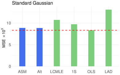
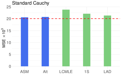
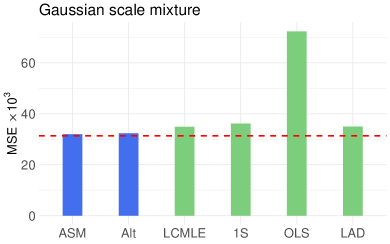
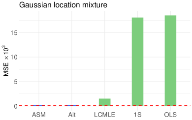
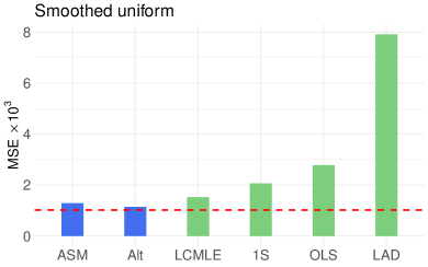
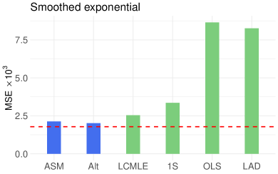
Figure 7: Plots of the average squared error loss ($\times 10^{3}$) of different estimators for noise distributions (i)–(vi), with $n=600$ and $d=6$. In each plot, the red dashed line indicates the corresponding value for the oracle convex $M$-estimator, and we omit the estimators that have very large estimation error (see Table 1 for full details).

We compared the performance of two versions of our procedure with an oracle approach and four existing methods. The first variant of our procedure, which we refer to as ASM (antitonic score matching) in all of the plots, is as described in Section 3, except that we do not perform sample splitting, cross-fitting or truncation of the initial score estimates. These devices are convenient for theoretical analysis but not essential in practice. More precisely, ASM first constructs a pilot estimator $(\bar{\theta}_{n},\bar{\mu}_{n})$, and then uses the vector of residuals $\bigl{(}\hat{\varepsilon}_{1},\ldots,\hat{\varepsilon}_{n}\bigr{)}$, where $\hat{\varepsilon}_{i}:=Y_{i}-\bar{\mu}_{n}-\tilde{X}_{i}^{\top}\bar{\theta}_{n}$, to obtain an initial kernel-based score estimator $\tilde{\psi}_{n}$, formed using a Gaussian kernel and the default Silverman’s choice of bandwidth (Silverman,, 1986, p. 48). Following Step 3^′ in Section 3.2, we estimate the antitonic projected score and the corresponding convex loss function by $\hat{\psi}_{n}:=\widehat{\mathcal{M}}_{\mathrm{R}}(\tilde{\psi}_{n}\circ\tilde{F}_{n}^{-1})\circ\tilde{F}_{n}$ and $\hat{\ell}_{n}$ respectively, where $\tilde{F}_{n}$ denotes the distribution function associated with the kernel density estimate. Finally, we use Newton’s algorithm to compute our semiparametric estimator

$$\hat{\theta}_{n}^{\mathrm{ASM}}\in\operatorname*{argmin}_{\theta\in\mathbb{R}^{d-1}}\sum_{i=1}^{n}\hat{\ell}_{n}\bigl{(}Y_{i}-\bar{\mu}_{n}-\bar{X}_{n}^{\top}\bar{\theta}_{n}-(\tilde{X}_{i}-\bar{X}_{n})^{\top}\theta\bigr{)},$$

where $\bar{X}_{n}:=n^{-1}\sum_{i=1}^{n}\tilde{X}_{i}$.

In the second version of our procedure, which we refer to as Alt in our plots, we implement the empirical analogue of the alternating optimisation procedure described at the beginning of Section 3. We start with an uninformative initialiser $(\hat{\theta}_{n}^{(0)},\hat{\mu}_{n}^{(0)})=(0,0)\in\mathbb{R}^{d-1}\times\mathbb{R}$, and then alternate between the following steps for $t\in\mathbb{N}$:

1. Compute residuals $\hat{\varepsilon}_{i}^{(t-1)}:=Y_{i}-\hat{\mu}_{n}^{(t-1)}-\tilde{X}_{i}^{\top}\hat{\theta}_{n}^{(t-1)}$ for $i\in[n]$ and hence estimate the antitonic projected score $\hat{\psi}_{n}^{(t-1)}$ and the corresponding convex loss $\hat{\ell}_{n}^{(t-1)}$ as for ASM.

2. Update $(\hat{\theta}_{n}^{(t)},\hat{\mu}_{n}^{(t)})\in\operatorname*{argmin}_{(\theta,\mu)\in\mathbb{R}^{d-1}\times\mathbb{R}}\sum_{i=1}^{n}\hat{\ell}_{n}^{(t-1)}(Y_{i}-\mu-\tilde{X}_{i}^{\top}\theta)$.

We iterate these steps until convergence of the empirical score matching objective

$$\hat{D}_{n}(\hat{\psi}_{n}^{(t)};\hat{\varepsilon}_{1}^{(t)},\dotsc,\hat{\varepsilon}_{n}^{(t)})=\frac{1}{n}\sum_{i=1}^{n}\bigl{\{}\hat{\psi}_{n}^{(t)}(\hat{\varepsilon}_{i}^{(t)})+2(\hat{\psi}_{n}^{(t)})^{\prime}(\hat{\varepsilon}_{i}^{(t)})\bigr{\}}$$

defined in (24). We note that the iterates $\hat{\mu}_{n}^{(t)}$ and $\hat{\psi}_{n}^{(t)}$ are not guaranteed to converge due to non-identifiability of the intercept term $\mu_{0}$ in (35), but $\hat{\theta}_{n}^{(t)}$ and the score matching objective values did indeed converge in all of our experiments.

The alternative approaches that we consider are as follows:

• Oracle: The $M$-estimator $\hat{\theta}_{n}^{\mathrm{oracle}}$, where

  $$\begin{pmatrix}\hat{\theta}_{n}^{\mathrm{oracle}}\\ \hat{\mu}_{n}^{\mathrm{oracle}}\end{pmatrix}\in\operatorname*{argmin}_{(\theta,\mu)\in\mathbb{R}^{d-1}\times\mathbb{R}}\;\sum_{i=1}^{n}\ell_{0}^{*}(Y_{i}-\mu-\tilde{X}_{i}^{\top}\theta)$$

  is defined with respect to the optimal convex loss function $\ell_{0}^{*}$. Although $\hat{\theta}_{n}^{\mathrm{oracle}}$ asymptotically attains antitonic efficiency in the sense of Theorem 16, it is not a valid estimator in our semiparametric framework since it requires knowledge of $p_{0}$.

• LAD: The least absolute deviation estimator $\hat{\theta}_{n}^{\mathrm{LAD}}$, where

  $$\begin{pmatrix}\hat{\theta}_{n}^{\mathrm{LAD}}\\ \hat{\mu}_{n}^{\mathrm{LAD}}\end{pmatrix}\in\operatorname*{argmin}_{(\theta,\mu)\in\mathbb{R}^{d-1}\times\mathbb{R}}\;\sum_{i=1}^{n}|Y_{i}-\mu-\tilde{X}_{i}^{\top}\theta|.$$

• OLS: The ordinary least squares estimator $\hat{\theta}_{n}^{\mathrm{OLS}}$, where

  $$\begin{pmatrix}\hat{\theta}_{n}^{\mathrm{OLS}}\\ \hat{\mu}_{n}^{\mathrm{OLS}}\end{pmatrix}\in\operatorname*{argmin}_{(\theta,\mu)\in\mathbb{R}^{d-1}\times\mathbb{R}}\;\sum_{i=1}^{n}(Y_{i}-\mu-\tilde{X}_{i}^{\top}\theta)^{2}.$$

• 1S: The semiparametric one-step method, where we start with a pilot estimator $(\bar{\theta}_{n},\bar{\mu}_{n})$, compute a (not necessarily decreasing) nonparametric score estimate, and then update $\bar{\theta}_{n}$ with a single Newton step instead of solving the estimating equations exactly. Our implementation follows van der Vaart, (1998, Chapter 25.8): we split the data into two folds of equal size indexed by $I_{1}$ and $I_{2}$, and then use the residuals $\hat{\varepsilon}_{i}:=Y_{i}-\tilde{X}_{i}^{\top}\bar{\theta}_{n}-\bar{\mu}_{n}$ for $i\in I_{1}$ and $i\in I_{2}$ separately to obtain kernel density estimates $\hat{p}_{n,1},\hat{p}_{n,2}$ of $p_{0}$ (constructed as for ASM). Defining the score estimates $\hat{\psi}_{n,j}:=\hat{p}_{n,j}^{\prime}/\hat{p}_{n,j}$ for $j\in\{1,2\}$, we output the cross-fitted estimator $\hat{\theta}_{n}^{\mathrm{1S}}$, where

  $$\begin{pmatrix}\hat{\theta}_{n}^{\mathrm{1S}}\\ \hat{\mu}_{n}^{\mathrm{1S}}\end{pmatrix}:=\begin{pmatrix}\bar{\theta}_{n}\\ \bar{\mu}_{n}\end{pmatrix}- \biggl{(}\sum_{i\in I_{1}}\hat{\psi}_{n,2}(\hat{\varepsilon}_{i})^{2}X_{i}X_{i}^{\top}+\sum_{i\in I_{2}}\hat{\psi}_{n,1}(\hat{\varepsilon}_{i})^{2}X_{i}X_{i}^{\top}\biggr{)}^{-1}$$

  $$\hskip 142.26378pt\biggl{(}\sum_{i\in I_{1}}\hat{\psi}_{n,2}(\hat{\varepsilon}_{i})X_{i}+\sum_{i\in I_{2}}\hat{\psi}_{n,1}(\hat{\varepsilon}_{i})X_{i}\biggr{)}.$$

• LCMLE: We estimate the error density $p_{0}$ using the log-concave maximum likelihood estimator (Cule et al.,, 2010; Dümbgen et al.,, 2011, 2013). More precisely, again writing $\mathcal{P}_{\mathrm{LC}}$ for the set of univariate log-concave densities, start with a pilot estimator $(\hat{\theta}_{n}^{(0)},\hat{\mu}_{n}^{(0)})$ and alternate the following two steps for $t\in\mathbb{N}$:

  $$\hat{p}_{n}^{(t)} \in\operatorname*{argmax}_{p\in\mathcal{P}_{\mathrm{LC}}}\;\sum_{i=1}^{n}\,\log p(Y_{i}-\hat{\mu}_{n}^{(t-1)}-\tilde{X}_{i}^{\top}\hat{\theta}_{n}^{(t-1)})$$

  $$\begin{pmatrix}\hat{\theta}_{n}^{(t)}\\ \hat{\mu}_{n}^{(t)}\end{pmatrix} \in\operatorname*{argmax}_{(\theta,\mu)\in\mathbb{R}^{d-1}\times\mathbb{R}}\;\sum_{i=1}^{n}\,\log\hat{p}_{n}^{(t)}(Y_{i}-\mu-\tilde{X}_{i}^{\top}\theta).$$

Where required, we took the pilot estimator to be the least absolute deviation estimator for all methods except in the Gaussian location mixture setting (iv). Here, we chose $(\hat{\theta}_{n}^{\mathrm{OLS}},\hat{\mu}_{n}^{\mathrm{OLS}})$ to be the pilot estimator since $p_{0}(0)$ is close to 0 and hence $V_{p_{0}}(\psi)=1/\bigl{(}4p_{0}(0)^{2}\bigr{)}$ is very large for $\hat{\theta}_{n}^{\mathrm{LAD}}$, where $\psi(\cdot)=-\operatorname{sgn}(\cdot)$.

$n$	600	1200	2400
ASM	0.26	0.61	1.93
Alt	4.35	9.99	27.85
LCMLE	0.64	2.21	8.34
1S	0.10	0.15	0.29

Standard Gaussian

$n$	600	1200	2400
ASM	0.27	0.61	1.81
Alt	5.03	10.52	28.64
LCMLE	0.71	1.36	2.72
1S	0.11	0.15	0.29

Gaussian scale mixture

$n$	600	1200	2400
ASM	0.21	0.58	1.96
Alt	1.84	3.72	11.36
LCMLE	3.15	7.09	9.29
1S	0.12	0.15	0.29

Gaussian location mixture

Table 2: Mean execution time in seconds for different semiparametric estimators when $d=100$.

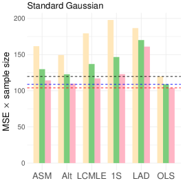
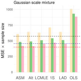
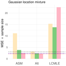
Figure 8: Plot of $n\times(\text{average squared loss})$ for different estimators, with $d=100$ and sample sizes $n\in\{600,1200,2400\}$ corresponding to the yellow, green, and pink bars respectively. The black, blue and red dashed lines indicate the values of $n\times(\text{average squared loss})$ for the oracle convex $M$-estimator when $n=600,1200,2400$ respectively.

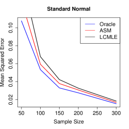
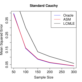
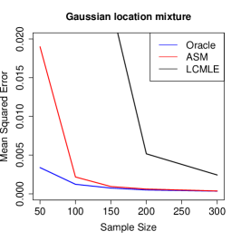
Figure 9: Comparison of the mean squared errors of different convex $M$-estimators for sample sizes $n\in\{50,100,150,200,250,300\}$ and $d=6$.

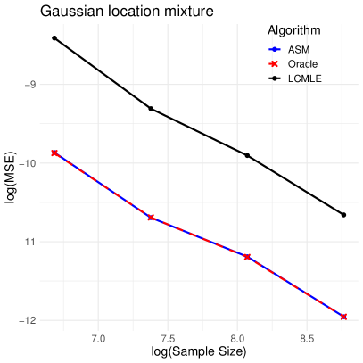
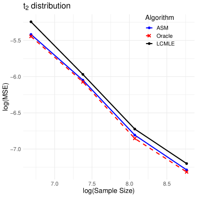
Figure 10: Log-log plots of the average squared error loss against sample size for three convex $M$-estimators. In each experiment, we set $n\in\{800,1600,3200,6400\}$ and $d=2$.

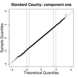
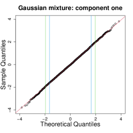
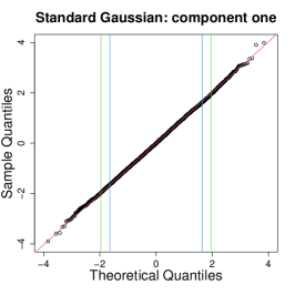
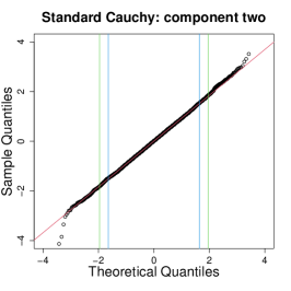
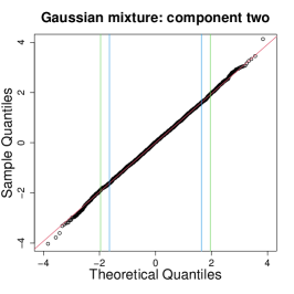
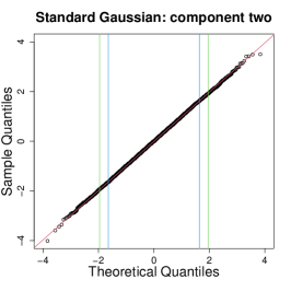
Figure 11: Q-Q plots of the standardised errors of estimates of two components of $\theta_{0}$. The blue and green vertical lines mark the 90% and 95% theoretical quantiles respectively. In each experiment, we set $n=600$ and $d=4$, and perform 8000 repetitions.

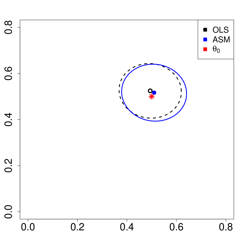
(a) Standard normal

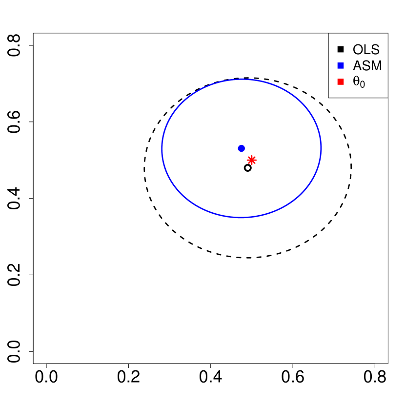
(b) Gaussian mixture

Figure 12: The projection of the $95\%$ confidence ellipsoid of $\hat{\theta}^{\mathrm{ASM}}$ onto the first two dimensions (blue) and the projection of the $95\%$ confidence ellipsoid of $\hat{\theta}_{n}^{\mathrm{OLS}}$ onto the first two dimensions (black dashed). The blue dot, black circle and red star correspond to $\hat{\theta}^{\mathrm{ASM}}$, $\hat{\theta}_{n}^{\mathrm{OLS}}$, and $\theta_{0}$ respectively.

	$\theta_{0,1}$	$\theta_{0,2}$	$\theta_{0,3}$
95% CI	0.965	0.965	0.964
90% CI	0.924	0.925	0.924

Standard Cauchy

	$\theta_{0,1}$	$\theta_{0,2}$	$\theta_{0,3}$
95% CI	0.952	0.955	0.955
90% CI	0.905	0.908	0.908

Gaussian mixture

	$\theta_{0,1}$	$\theta_{0,2}$	$\theta_{0,3}$
95% CI	0.950	0.954	0.952
90% CI	0.903	0.902	0.901

Standard Gaussian

Table 3: Empirical coverage of the confidence intervals for each coordinate of $\theta_{0}$. In each experiment, we set $n=600$ and $d=4$, and perform 8000 repetitions.

	Cauchy	Mixture	Gaussian
$i^{*}(p_{0})$	0.44	0.46	1.0
RMSE($\hat{\jmath}_{n}$)	0.01	0.05	0.1

(a) Root mean squared errors of $\hat{\jmath}_{n}$.

	Cauchy	Mixture	Gaussian
$\dfrac{\mathrm{Vol}(\hat{C}_{n}^{\mathrm{ASM}})}{\mathrm{Vol}(\hat{C}_{n}^{\mathrm{OLS}})}$	0.001	0.49	1.14

(b) Mean ratio of volumes of $\hat{C}_{n}^{\mathrm{ASM}}$ and $\hat{C}_{n}^{\mathrm{OLS}}$.

Table 4: Accuracy of estimates of the antitonic information, and comparison of the volumes of the two confidence ellipsoids. In each experiment, we set $n=600$ and $d=4$, and perform 8000 repetitions.

4.1 Estimation accuracy

In all of the experiments in this subsection, we set $d=6$, $\mu_{0}=2$ and drew $\theta_{0}$ uniformly at random from the centred Euclidean sphere in $\mathbb{R}^{d-1}$ of radius 3. For each of the estimators above, the average squared Euclidean norm errors $\|{\hat{\theta}_{n}-\theta_{0}}\|^{2}$ were computed over 200 repetitions. In the first experiment, we consider each error distribution in turn and compare the average squared estimation error when $n=600$. The results are presented in Table 1 and Figure 7. We observe that our proposed procedures ASM and Alt have the lowest estimation error except in the case of standard Gaussian error, where OLS coincides with the oracle convex loss estimator and has a slightly lower estimation error. It is interesting that the one-step estimator (1S) can perform very poorly in finite samples, and in particular, may barely improve on its initialiser. In all settings considered, ASM and Alt have comparable error.

Next, we investigate the running time and estimation accuracy of the semiparametric estimators ASM, Alt, LCMLE and 1S for moderately large sample sizes $n\in\{600,1200,2400\}$ and dimension $d=100$. We consider in turn the error distributions (i), (iii) and (iv); see Table 2 and Figure 8. We see that ASM in particular is competitive in terms of its running time, and that the performance of our procedures does not deteriorate relative to its competitors for this larger choice of $d$.

Our third numerical experiment demonstrates that the estimation error of ASM is comparable to that of the oracle convex $M$-estimator even for small sample sizes. For $n\in\{50,100,150,200,300\}$ and $d=6$, and error distributions (i), (ii) and (iv), we record in Figure 9 the average estimation error of Oracle, ASM, and LCMLE. With the exception of the smallest sample size $n=50$ in the Gaussian location mixture setting, the estimation error of ASM tracks that of the oracle very closely; on the other hand, LCMLE is somewhat suboptimal, particularly in the Gaussian location mixture setting.

Finally in this subsection, we verify empirically the suboptimality of LCMLE relative to ASM for larger sample sizes. We let $d=2$ and $n\in\{800,1600,3200,6400\}$, and consider error distribution (iv) above as well as the $t_{2}$ distribution (Example 26). We include the $t_{2}$ distribution in place of the standard Cauchy because when $P_{0}$ does not have a finite first moment, its population level log-concave maximum likelihood projection does not exist (and indeed we found empirically that LCMLE was highly unstable in the Cauchy setting). Figure 10 displays the average squared error loss of the oracle convex $M$-estimator, ASM, and LCMLE. We see that the relative efficiency of ASM with respect to Oracle approaches 1 as $n$ increases, while LCMLE has an efficiency gap that does not vanish even for large $n$, in agreement with the asymptotic calculation in Example 26.

4.2 Inference

In this subsection, we assess the finite-sample performance of the inferential procedures for $\theta_{0}$ described in Section 3.3, but do not perform sample splitting or cross-fitting. Here, we instead estimate the antitonic information $i^{*}(p_{0})$ by

$$\hat{\jmath}_{n}:=\frac{1}{n}\sum_{i=1}^{n}\hat{\psi}_{n}(\hat{\varepsilon}_{i})^{2},$$

rather than $\hat{\imath}_{n}$, where $\hat{\varepsilon}_{i}:=Y_{i}-\bar{\mu}_{n}-\tilde{X}_{i}^{\top}\bar{\theta}_{n}$ for $i\in[n]$ is the $i$th residual of the pilot estimator $(\bar{\theta}_{n},\bar{\mu}_{n})$. We then compute $\tilde{\mathcal{J}}_{n}:=\frac{\tilde{\jmath}_{n}}{n}\sum_{i=1}^{n}(\tilde{X}_{i}-\bar{X}_{n})(\tilde{X}_{i}-\bar{X}_{n})^{\top}$.

We first verify that the standardised error vector $\sqrt{n}\tilde{\mathcal{J}}_{n}^{1/2}(\hat{\theta}_{n}^{\mathrm{ASM}}-\theta_{0})$ has a distribution very close to $N_{d-1}(0,I_{d-1})$ under three different noise distributions: standard Gaussian, standard Cauchy, and the Gaussian mixture $P_{0}=\frac{2}{3}N(0,1)+\frac{1}{3}N\bigl{(}\frac{1}{2},9\bigr{)}$. Setting $n=600$ and $d=4$, we present the Q-Q plot for 8000 repetitions in Figure 11. Moreover, Table 4(a) demonstrates that the average squared estimation error $\bigl{(}\hat{\jmath}_{n}-i^{*}(p_{0})\bigr{)}^{2}$ is small.

Next, we show that the empirical coverage of the confidence ellipsoid

$$\hat{C}_{n}^{\mathrm{ASM}}:=\bigl{\{}v\in\mathbb{R}^{d-1}:n(\hat{\theta}_{n}^{\mathrm{ASM}}-v)^{\top}\tilde{\mathcal{J}}_{n}(\hat{\theta}_{n}^{\mathrm{ASM}}-v)\leq\chi^{2}_{d-1}(\alpha)\bigr{\}}$$

is close to the nominal level $1-\alpha$ when $n=600$. Indeed, for the standard Gaussian and Gaussian mixture noise distributions above, Table 3 reveals that we maintain nominal coverage while for standard Cauchy errors, our confidence set is slightly conservative. We also compare the volume of $\hat{C}_{n}^{\mathrm{ASM}}$ with that of the OLS confidence ellipsoid

$$\hat{C}_{n}^{\mathrm{OLS}}:=\bigl{\{}v\in\mathbb{R}^{d-1}:n(\hat{\theta}_{n}^{\mathrm{OLS}}-v)^{\top}\hat{I}_{n}^{\mathrm{OLS}}(\hat{\theta}_{n}^{\mathrm{OLS}}-v)\leq\chi^{2}_{d-1}(\alpha)\bigr{\}},$$

where $\hat{I}_{n}^{\mathrm{OLS}}:=n^{-1}\sum_{i=1}^{n}\hat{\sigma}^{-2}_{n}(\tilde{X}_{i}-\bar{X}_{n})(\tilde{X}_{i}-\bar{X}_{n})^{\top}$ and $\hat{\sigma}_{n}^{2}:=n^{-1}\sum_{i=1}^{n}(Y_{i}-\hat{\mu}^{\mathrm{OLS}}_{n}-\tilde{X}_{i}^{\top}\hat{\theta}_{n}^{\mathrm{OLS}})^{2}$. We plot examples of $\hat{C}_{n}^{\mathrm{ASM}}$ and $\hat{C}_{n}^{\mathrm{OLS}}$ in Figure 12, and compute the average ratio of their volumes in Table 4(b). The ASM ellipsoid is appreciably smaller than the OLS ellipsoid except when the noise distribution is standard Gaussian, in which case the OLS ellipsoid is slightly smaller.

5 Discussion

Despite the Gauss–Markov theorem, one of the messages of this paper is that the success of ordinary least squares is relatively closely tied to Gaussian or near-Gaussian error distributions. Our antitonic score matching approach represents a middle ground that frees the practitioner from the Gaussian straitjacket while retaining the convenience and stability of working with convex loss functions. The Fisher divergence projection framework brings together previously disparate ideas on shape-constrained estimation, score matching, information theory and classical robust statistics. Given the prevalence of procedures in statistics and machine learning that are constructed as optimisers of pre-specified loss functions, we look forward to seeing how related insights may lead to more flexible, data-driven approaches that combine robustness and efficiency.

Acknowledgements: The authors thank Cun-Hui Zhang for helpful discussions. The research of YCK and MX was supported by National Science Foundation grants DMS-2311299 and DMS-2113671; OYF and RJS were supported by Engineering and Physical Sciences Research Council Programme Grant EP/N031938/1, while RJS was also supported by European Research Council Advanced Grant 101019498.

6 Appendix

6.1 Proofs for Section 2

Throughout this subsection, we work in the setting of Lemmas 1 and 5. Moreover, define $Q_{0}(u):=\sup\{z\in[-\infty,\infty]:F_{0}(z)\leq u\}$ for $u\in[0,1]$. Then $z_{\min}:=\inf(\operatorname{supp}p_{0})=Q_{0}(0)$ and $z_{\max}:=\sup(\operatorname{supp}p_{0})=F_{0}^{-1}(1)$, and $\mathcal{S}_{0}=\{z\in\mathbb{R}:F_{0}(z)\in(0,1)\}$.

Proof of Lemma 1.

If $F_{0}^{-1}(v)<Q_{0}(v)$ for some $v\in[0,1]$, then because $p_{0}(\pm\infty)=0$ and $p_{0},F_{0}$ are both continuous, we have $p_{0}(z)=0$ for all $z\in[F_{0}^{-1}(v),Q_{0}(v)]=\{z\in[-\infty,\infty]:F_{0}(z)=v\}$. Therefore, $p_{0}(z)=J_{0}\bigl{(}F_{0}(z)\bigr{)}$ for all $z\in\mathbb{R}$ and $J_{0}(v)=p_{0}\bigl{(}F_{0}^{-1}(v)\bigr{)}=p_{0}\bigl{(}Q_{0}(v)\bigr{)}$ for all $v\in[0,1]$, with $J_{0}(0)=J_{0}(1)=0$. Since $\lim_{u\nearrow v}F_{0}^{-1}(u)=F_{0}^{-1}(v)$ and $\lim_{u\searrow v}F_{0}^{-1}(u)=Q_{0}(v)$ for all $v\in[0,1]$, it follows from the continuity of $p_{0}$ on $[-\infty,\infty]$ that $J_{0}$ is continuous on $[0,1]$. Moreover, the least concave majorant $\hat{J}_{0}$ satisfies $\sup_{u\in[0,1]}\hat{J}_{0}(u)=\sup_{u\in[0,1]}J_{0}(u)<\infty$ and

$$\hat{J}_{0}(0)=J_{0}(0)=0=J_{0}(1)=\hat{J}_{0}(1).$$ (42)

In particular, $\hat{J}_{0}$ is concave and bounded, so it is also continuous on $[0,1]$. By Rockafellar, (1997, Theorem 24.1), the right derivative $\hat{J}_{0}^{(\mathrm{R})}$ is decreasing and right-continuous on $[0,1)$, with $\hat{J}_{0}^{(\mathrm{R})}(u)\in\mathbb{R}$ for all $u\in(0,1)$. Thus, $\psi_{0}^{*}$ is finite-valued on $\mathcal{S}_{0}$. If $z_{n}\searrow z$ for some $z\in\mathbb{R}$, then either $u_{n}:=F_{0}(z_{n})\searrow F_{0}(z)=:u<1$ or $u_{n}=u=1$ for all $n$. In both cases, $\psi_{0}^{*}(z_{n})=\hat{J}_{0}^{(\mathrm{R})}(u_{n})\nearrow\hat{J}_{0}^{(\mathrm{R})}(u)=\psi_{0}^{*}(z)$, so $\psi_{0}^{*}$ is right-continuous as a function from $\mathbb{R}$ to $[-\infty,\infty]$. Since $F_{0}$ is increasing, $\psi_{0}^{*}$ is decreasing.

We have $z_{\min}=\inf\{z\in\mathbb{R}:F_{0}(z)>0\}$ and $\log F_{0}(z)\searrow-\infty$ as $z\searrow z_{\min}$. Thus, if $z_{\min}>-\infty$, then

$$\limsup_{u\searrow 0}\frac{J_{0}(u)}{u}=\limsup_{z\searrow z_{\min}}\frac{J_{0}\bigl{(}F_{0}(z)\bigr{)}}{F_{0}(z)}=\limsup_{z\searrow z_{\min}}\frac{p_{0}(z)}{F_{0}(z)}=\limsup_{z\searrow z_{\min}}\,(\log F_{0})^{\prime}(z)=\infty,$$ (43)

where the final equality follows from the mean value theorem. Together with Lemma 46, this implies that $\psi_{0}^{*}(z)=\hat{J}_{0}^{(\mathrm{R})}(0)=\infty$ for all $z\leq z_{\min}$. Similarly, if $z_{\max}<\infty$, then $\psi_{0}^{*}(z)=\hat{J}_{0}^{(\mathrm{R})}(1)=-\infty$ for all $z\geq z_{\max}$. Therefore, in all cases, $\psi_{0}^{*}(z)\in\mathbb{R}$ if and only if $z\in\mathcal{S}_{0}$. ∎

The next lemma characterises precisely the class of density quantile functions of uniformly continuous densities on $\mathbb{R}$, and shows explicitly how to recover a density from a continuous density quantile function that is strictly positive on $(0,1)$.

Lemma 19.

A function $J\colon[0,1]\to[0,\infty)$ is the density quantile function of a uniformly continuous density on $\mathbb{R}$ if and only if

$$\text{ $J$ is continuous on $[0,1]$ with $J(0)=J(1)=0$ and }Q_{J}(u):=\int_{1/2}^{u}\frac{1}{J}<\infty$$ (44)

for all $u\in(0,1)$. In this case, $Q_{J}$ is a strictly increasing, continuously differentiable bijection from $(0,1)$ to $\bigl{(}Q_{J}(0),Q_{J}(1)\bigr{)}$, and the function $p_{J}\colon\mathbb{R}\to\mathbb{R}$ given by

$$p_{J}(z):=\begin{cases}(Q_{J}^{-1})^{\prime}(z)\;&\text{for }z\in\bigl{(}Q_{J}(0),Q_{J}(1)\bigr{)}\\ 0\;&\text{otherwise}\end{cases}$$

is a uniformly continuous density with corresponding density quantile function $J$. If in addition $J>0$ on $(0,1)$, then a density $p_{0}$ has density quantile function $J$ if and only if $p_{0}(\cdot)=p_{J}(\cdot-\mu)$ for some $\mu\in\mathbb{R}$.

Proof.

If $p_{0}$ is a uniformly continuous density with density quantile function $J_{0}=p_{0}\circ F_{0}^{-1}$, then Lemma 1 shows that $J_{0}$ is continuous with $J_{0}(0)=J_{0}(1)=0$. Introducing $U\sim U(0,1)$ and $Z:=F_{0}^{-1}(U)\sim P_{0}$, we have $p_{0}(Z)=J_{0}(U)$ and $\mathbb{P}\bigl{(}J_{0}(U)=0\bigr{)}=\mathbb{P}\bigl{(}p_{0}(Z)=0\bigr{)}=0$. Moreover, since $F_{0}$ is continuous, $(F_{0}\circ F_{0}^{-1})(u)=u$ for all $u\in(0,1)$, so $U=F_{0}(Z)$. Therefore,

$$\int_{1/2}^{u}\frac{1}{J_{0}}=\mathbb{E}\biggl{(}\frac{1}{J_{0}(U)}\mathbbm{1}_{\{U\in[1/2,u)\}}\biggr{)}=\mathbb{E}\biggl{(}\frac{1}{p_{0}(Z)}\mathbbm{1}_{\{Z\in[F_{0}^{-1}(1/2),F_{0}^{-1}(u))\}}\biggr{)}\leq F_{0}^{-1}(u)-F_{0}^{-1}\Bigl{(}\frac{1}{2}\Bigr{)}<\infty$$ (45)

for $u\in[1/2,1)$, with equality if and only if $p_{0}(z)>0$ Lebesgue almost everywhere on $\bigl{[}F_{0}^{-1}(1/2),F_{0}^{-1}(u)\bigr{)}$. Similarly, for $u\in(0,1/2]$, (45) remains true, with an analogous equality condition.

Conversely, if $J\colon[0,1]\to\mathbb{R}$ satisfies (44), then $Q_{J}$ is strictly increasing with $Q_{J}^{\prime}(u)=1/J(u)$ for all $u\in(0,1)$. Thus, $Q_{J}$ is a continuously differentiable bijection from $(0,1)$ to $\bigl{(}Q_{J}(0),Q_{J}(1)\bigr{)}$, so by the inverse function theorem, $F_{J}:=Q_{J}^{-1}\colon\bigl{(}Q_{J}(0),Q_{J}(1)\bigr{)}\to(0,1)$ is a well-defined, continuously differentiable bijection with derivative $p_{J}:=F_{J}^{\prime}=1/(Q_{J}^{\prime}\circ F_{J})=J\circ F_{J}$ satisfying $J=p_{J}\circ F_{J}^{-1}$ on $(0,1)$. We have $\lim_{z\searrow Q_{J}(0)}F_{J}(z)=0$ and $\lim_{z\nearrow Q_{J}(1)}F_{J}(z)=1$, while $\lim_{z\searrow Q_{J}(0)}p_{J}(z)=\lim_{z\nearrow Q_{J}(1)}p_{J}(z)=0$ since $J$ is continuous at $0$ and $1$. Therefore, setting $p_{J}(z)=0$ for $z\in\mathbb{R}\setminus\bigl{(}Q_{J}(0),Q_{J}(1)\bigr{)}$, we conclude that $p_{J}$ is a uniformly continuous density on $\mathbb{R}$ with corresponding distribution function $F_{J}$, quantile function $Q_{J}$ and density quantile function $J$. Moreover, for every $\mu\in\mathbb{R}$, the density $p_{J}(\cdot-\mu)$ also has density quantile function $J$.

Finally, if $p_{0}$ is a uniformly continuous density with density quantile function $J=p_{0}\circ F_{0}^{-1}>0$ on $(0,1)$, then for every $u\in(0,1)$, equality holds in (44) and hence

$$Q_{J}(u)=\int_{1/2}^{u}\frac{1}{J}=F_{0}^{-1}(u)-F_{0}^{-1}\Bigl{(}\frac{1}{2}\Bigr{)}.$$

Therefore, letting $\mu:=F_{0}^{-1}(1/2)$, we deduce that $p_{0}(\cdot)=p_{J}(\cdot-\mu)$, which completes the proof. ∎

Lemma 20.

Let $\mathcal{T}$ be as in Proposition 9(a). If $t\in\mathcal{T}$, then $p_{0}(t)=\hat{J}_{0}\bigl{(}F_{0}(t)\bigr{)}>0$.

Proof.

Since $\hat{J}_{0}$ is a non-negative concave function, we must have $\hat{J}_{0}>0$ on $(0,1)$, as otherwise $J_{0}=\hat{J}_{0}=0$ and hence $p_{0}=J_{0}\circ F_{0}=0$ on $\mathbb{R}$ by Lemma 1, which is a contradiction. Moreover, $\psi_{0}^{*}(t)\in\mathbb{R}$, so again by Lemma 1, $t\in\mathcal{S}_{0}$. Thus, $v:=F_{0}(t)\in(0,1)$ and $p_{0}(t)=(J_{0}\circ F_{0})(t)=J_{0}(v)$. Suppose for a contradiction that $J_{0}(v)<\hat{J}_{0}(v)$. Then by Lemma 45 and the fact that $J_{0}$ and $\hat{J}_{0}$ are continuous at $v$, there exists $\delta>0$ such that $\hat{J}_{0}$ is affine on $[v-\delta,v+\delta]$. Thus, $\hat{J}_{0}^{(\mathrm{R})}$ is constant on $[v-\delta,v+\delta)$, so $\psi_{0}^{*}=\hat{J}_{0}^{(\mathrm{R})}\circ F_{0}$ is constant on the open interval $\bigl{(}Q_{0}(v-\delta),F_{0}^{-1}(v+\delta)\bigr{)}$, which contains $t$. This contradicts the definition of $\mathcal{T}$, so $p_{0}(t)=J_{0}(v)=\hat{J}_{0}(v)>0$, as required. ∎

Lemma 21.

If $\psi\in\Psi_{\downarrow}(p_{0})$ satisfies $\psi=\psi_{0}^{*}$ $P_{0}$-almost everywhere, then in fact $\psi=\psi_{0}^{*}$ on $\mathbb{R}$.

Proof.

First consider $z\in\mathcal{S}_{0}$, let $u:=F_{0}(z)\in(0,1)$ and let $u_{1}:=\inf\bigl{\{}v\in[0,1]:\hat{J}_{0}^{(\mathrm{R})}(v)=\hat{J}_{0}^{(\mathrm{R})}(u)\bigr{\}}$. Then $\hat{J}_{0}^{(\mathrm{R})}(u_{1})=\hat{J}_{0}^{(\mathrm{R})}(u)$ by the right-continuity of $\hat{J}_{0}^{(\mathrm{R})}$. Moreover, define $z_{1}:=F_{0}^{-1}(u_{1})$ and $z_{2}:=Q_{0}(u)$, so that $z_{1}\leq z\leq z_{2}$ and

$$F_{0}(z_{1}-\delta)<u_{1}=F_{0}(z_{1})\leq F_{0}(z_{2})=u<F_{0}(z_{2}+\delta)$$

for all $\delta>0$. Then $\psi_{0}^{*}(z_{1}-\delta)=\hat{J}_{0}^{(\mathrm{R})}\bigl{(}F_{0}(z_{1}-\delta)\bigr{)}>\hat{J}_{0}^{(\mathrm{R})}(u_{1})=\psi_{0}^{*}(z_{1})$ for all such $\delta$, so $z_{1}\in\mathcal{T}$ and hence $p_{0}(z_{1})>0$ by Lemma 20. It follows that $P_{0}\bigl{(}[z_{j},z_{j}+\delta)\bigr{)}>0$ for $j\in\{1,2\}$, so because $\psi$ and $\psi_{0}^{*}$ are decreasing, right-continuous functions that agree $P_{0}$-almost everywhere,

$$\psi(z)\leq\psi(z_{1})=\psi_{0}^{*}(z_{1})=\hat{J}_{0}^{(\mathrm{R})}(u_{1})=\hat{J}_{0}^{(\mathrm{R})}(u)=\psi_{0}^{*}(z_{2})=\psi(z_{2})\leq\psi(z).$$

Thus, $\psi(z)=\psi_{0}^{*}(z)$ for all $z\in\mathcal{S}_{0}$. Together with Lemma 1, this implies that $\lim_{z\searrow z_{\min}}\psi(z)=\lim_{z\searrow z_{\min}}\psi_{0}^{*}(z)=\infty$ and $\lim_{z\nearrow z_{\max}}\psi(z)=\lim_{z\nearrow z_{\max}}\psi_{0}^{*}(z)=-\infty$, so $\psi=\psi_{0}^{*}=\infty$ on $(-\infty,z_{\min}]$ and $\psi=\psi_{0}^{*}=-\infty$ on $[z_{\max},\infty)$. Thus, $\psi=\psi_{0}^{*}$ on $\mathbb{R}$, as required. ∎

Proof of Theorem 2.

Let $\chi_{t}:=\mathbbm{1}_{(-\infty,t)}\in\Psi_{\downarrow}(p_{0})$ for $t\in(\infty,\infty]$. Then, letting $U\sim U(0,1)$, we have $(F_{0}\circ F_{0}^{-1})(U)=U$, so

$$\int_{\mathbb{R}}\psi_{0}^{*}\chi_{t}\,dP_{0}=\int_{(-\infty,t)}(\hat{J}_{0}^{(\mathrm{R})}\circ F_{0})\,dP_{0} =\mathbb{E}\bigl{\{}\bigl{(}\hat{J}_{0}^{(\mathrm{R})}\circ F_{0}\circ F_{0}^{-1}\bigr{)}(U)\,\mathbbm{1}_{\{F_{0}^{-1}(U)\leq t\}}\bigr{\}}$$

$$=\mathbb{E}\bigl{\{}\hat{J}_{0}^{(\mathrm{R})}(U)\,\mathbbm{1}_{\{U\leq F_{0}(t)\}}\bigr{\}}=\int_{0}^{F_{0}(t)}\hat{J}_{0}^{(\mathrm{R})}$$

$$=\hat{J}_{0}\bigl{(}F_{0}(t)\bigr{)}-\hat{J}_{0}(0)\geq J_{0}\bigl{(}F_{0}(t)\bigr{)}=p_{0}(t),$$

where the last two equalities are due to Rockafellar, (1997, Corollary 24.2.1) and Lemma 1 respectively. By (42) and Lemma 20, equality holds throughout in the final line if $F_{0}(t)\in\{0,1\}$ or $t\in\mathcal{T}$, so

$$\int_{\mathbb{R}}\psi_{0}^{*}\chi_{t}\,dP_{0}\,\begin{cases}\geq p_{0}(t)&\;\text{for all }t\in(\infty,\infty]\\ =p_{0}(t)&\;\text{for all }t\in(-\infty,z_{\min}]\cup[z_{\max},\infty]\cup\mathcal{T}.\end{cases}$$ (46)

(a) In particular, taking $t=\infty$, we have $\int_{\mathbb{R}}\psi_{0}^{*}\,dP_{0}=0$.

(b, c) Case 1: Suppose that $i^{*}(p_{0})=\int_{\mathbb{R}}(\psi_{0}^{*})^{2}\,dP_{0}<\infty$. Then $\psi_{0}^{*}\in\Psi_{\downarrow}(p_{0})$ since it is decreasing and right-continuous. For measurable functions $\psi$ on $\mathbb{R}$, we write $\|{\psi}\|\equiv\|{\psi}\|_{L^{2}(P_{0})}:=(\int_{\mathbb{R}}\psi^{2}\,dP_{0})^{1/2}$, and for $\psi_{1},\psi_{2}\in L^{2}(P_{0})$, denote by $\langle\psi_{1},\psi_{2}\rangle\equiv\langle\psi_{1},\psi_{2}\rangle_{L^{2}(P_{0})}:=\int_{\mathbb{R}}\psi_{1}\psi_{2}\,dP_{0}$ their $L^{2}(P_{0})$ inner product. Recalling that $D_{p_{0}}(\cdot\,,\lambda)$ is a convex (quadratic) function on the convex cone $\Psi_{\downarrow}(p_{0})$, we will deduce from (46) that $\psi_{0}^{*}$ satisfies the first-order stationarity condition

$$-\int_{\mathcal{S}_{0}}p_{0}\,d\psi\leq\int_{\mathbb{R}}\psi_{0}^{*}\psi\,dP_{0}=\langle\psi_{0}^{*},\psi\rangle\in\mathbb{R}$$ (47)

for all $\psi\in\Psi_{\downarrow}(p_{0})$, with equality when $\psi=\psi_{0}^{*}$. To see this, fix $t_{0}\in\mathcal{S}_{0}$ and define $g(z,t):=\mathbbm{1}_{\{z<t\leq t_{0}\}}-\mathbbm{1}_{\{t_{0}<t\leq z\}}$ for $z,t\in\mathbb{R}$. Then $g(\cdot,t)=\chi_{t}(\cdot)-\mathbbm{1}_{\{t>t_{0}\}}$ for all $t\in\mathbb{R}$ and $\psi(t_{0})-\psi(z)=\int_{\mathcal{S}_{0}}g(z,t)\,d\psi(t)$ for all $z\in\mathcal{S}_{0}$. Since $\int_{\mathbb{R}}|\psi_{0}^{*}||\psi(t_{0})-\psi|\,dP_{0}\leq\|{\psi_{0}^{*}}\|\bigl{(}|\psi(t_{0})|+\|{\psi}\|\bigr{)}<\infty$ and $\int_{\mathbb{R}}\psi_{0}^{*}\,dP_{0}=0$ by (46), we can apply Fubini’s theorem to obtain

$$\int_{\mathbb{R}}\psi_{0}^{*}\psi\,dP_{0} =\psi(t_{0})\int_{\mathbb{R}}\psi_{0}^{*}\,dP_{0}-\int_{\mathbb{R}}\psi_{0}^{*}(z)\int_{\mathcal{S}_{0}}g(z,t)\,d\psi(t)\,dP_{0}(z)=-\int_{\mathcal{S}_{0}}\int_{\mathbb{R}}\psi_{0}^{*}(z)\,g(z,t)\,dP_{0}(z)\,d\psi(t).$$ (48)

On the right-hand side of (48), the outer Lebesgue–Stieltjes integral is with respect to a negative measure, so it follows from (46) that

$$\int_{\mathcal{S}_{0}}\int_{\mathbb{R}}\psi_{0}^{*}(z)\,g(z,t)\,dP_{0}(z)\,d\psi(t) =\int_{(z_{\min},t_{0}]}\biggl{(}\int_{\mathbb{R}}\psi_{0}^{*}\chi_{t}\,dP_{0}\biggr{)}\,d\psi(t)+\int_{(t_{0},z_{\max})}\biggl{(}\int_{\mathbb{R}}\psi_{0}^{*}(\chi_{t}-1)\,dP_{0}\biggr{)}\,d\psi(t)$$

$$\leq\int_{(z_{\min},t_{0}]}p_{0}(t)\,d\psi(t)+\int_{(t_{0},z_{\max})}p_{0}(t)\,d\psi(t)=\int_{\mathcal{S}_{0}}p_{0}\,d\psi.$$ (49)

Together with (48), this proves the inequality (47) for all $\psi\in\Psi_{\downarrow}(p_{0})$. It remains to show that (47) holds with equality when $\psi=\psi_{0}^{*}$. Let $\nu^{*}$ for the Lebesgue–Stieltjes measure induced by $\psi_{0}^{*}$, so that the set $\mathcal{T}$ in Lemma 20 is the support of $\nu^{*}$. Then $\mathcal{T}^{c}$ is an open set with $\nu^{*}(\mathcal{T}^{c})=0$, so $\psi_{0}^{*}(t_{0})-\psi_{0}^{*}(z)=\int_{\mathcal{T}}g(z,t)\,d\psi_{0}^{*}(t)$ for all $z\in\mathbb{R}$. Thus, (48) holds for $\psi=\psi_{0}^{*}$ when the Lebesgue–Stieltjes integrals (with respect to $\nu^{*}$) are restricted to $\mathcal{S}_{0}\cap\mathcal{T}$. Moreover, (49) is still valid if we intersect the domains of all outer integrals with $\mathcal{T}$, again because $\nu^{*}(\mathcal{T}^{c})=0$. We established that (46) is an equality for all $t\in\mathcal{T}$, so (49) and hence (47) hold with equality when $\psi=\psi_{0}^{*}$.

For $\psi\in\Psi_{\downarrow}(p_{0})$, it follows from (47) that $\int_{\mathcal{S}_{0}}p_{0}\,d\psi>-\infty$ and hence $D_{p_{0}}(\psi,\lambda)\in\mathbb{R}$ for every $\lambda>0$, so

$$D_{p_{0}}(\psi,\lambda) =\int_{\mathbb{R}}(\psi-\lambda\psi_{0}^{*})^{2}\,dP_{0}+\int_{\mathbb{R}}(\lambda\psi_{0}^{*})^{2}\,dP_{0}+2\lambda\,\biggl{\{}\int_{\mathbb{R}}\psi_{0}^{*}(\psi-\lambda\psi_{0}^{*})\,dP_{0}+\int_{\mathcal{S}_{0}}p_{0}\,d\psi\biggr{\}}$$

$$\geq\int_{\mathbb{R}}(\psi-\lambda\psi_{0}^{*})^{2}\,dP_{0}-\lambda^{2}\int_{\mathbb{R}}(\psi_{0}^{*})^{2}\,dP_{0}$$ (50)

$$=\int_{\mathbb{R}}(\psi-\lambda\psi_{0}^{*})^{2}\,dP_{0}+\int_{\mathbb{R}}(\lambda\psi_{0}^{*})^{2}\,dP_{0}+2\lambda^{2}\int_{\mathcal{S}_{0}}p_{0}\,d\psi_{0}^{*}$$

$$=\int_{\mathbb{R}}(\psi-\lambda\psi_{0}^{*})^{2}\,dP_{0}+D_{p_{0}}(\lambda\psi_{0}^{*},\lambda)\geq D_{p_{0}}(\lambda\psi_{0}^{*},\lambda).$$

Thus, $\psi\in\operatorname*{argmin}_{\psi\in\Psi_{\downarrow}(p_{0})}D_{p_{0}}(\psi,\lambda)$ if and only if $\psi=\lambda\psi_{0}^{*}$ $P_{0}$-almost everywhere. By Lemma 21, this holds if and only if $\psi=\lambda\psi_{0}^{*}$ on $\mathbb{R}$, which proves the uniqueness assertion in (b).

Moreover, since $\hat{J}_{0}^{(\mathrm{R})}(0)=\lim_{u\searrow 0}\hat{J}_{0}^{(\mathrm{R})}(u)>0$ and $F_{0}(z)>0$ for all $z>Q_{0}(0)=z_{\min}$, we have $\int_{(z_{\min},z)}(\psi_{0}^{*})^{2}\,dP_{0}=\int_{(z_{\min},z)}(\hat{J}_{0}^{(\mathrm{R})}\circ F_{0})^{2}\,dP_{0}>0$ for all $z>z_{\min}$, so $i^{*}(p_{0})=\|{\psi_{0}^{*}}\|^{2}>0$. Now for $\psi\in\Psi_{\downarrow}(p_{0})$ such that $\int_{\mathbb{R}}\psi^{2}\,dP_{0}>0$, we have $-\int_{\mathcal{S}_{0}}p_{0}\,d\psi\geq 0$ since $\psi$ is decreasing. It follows from (47) and the Cauchy–Schwarz inequality that

$$V_{p_{0}}(\psi)=\frac{\int_{\mathbb{R}}\psi^{2}\,dP_{0}}{\bigl{(}\int_{\mathcal{S}_{0}}p_{0}\,d\psi\bigr{)}^{2}}\geq\frac{\|{\psi}\|^{2}}{\langle\psi_{0}^{*},\psi\rangle^{2}}\geq\frac{1}{\|{\psi_{0}^{*}}\|^{2}}=\frac{1}{i^{*}(p_{0})}\in(0,\infty),$$

with equality if and only if $\psi=\lambda\psi_{0}^{*}$ $P_{0}$-almost everywhere for some $\lambda>0$. By Lemma 21, this holds if and only if $\psi=\lambda\psi_{0}^{*}$ on $\mathbb{R}$, so the proof of (c) is complete.

Case 2: Suppose instead that $i^{*}(p_{0})=\int_{\mathbb{R}}(\psi_{0}^{*})^{2}\,dP_{0}=\infty$. For each $n\in\mathbb{N}$, define $\psi_{n}^{*}:=(\psi_{0}^{*}\wedge n)\vee(-n)$. This is bounded, decreasing and right-continuous, so $\psi_{n}^{*}\in\Psi_{\downarrow}(p_{0})$, and we claim that

$$-\int_{\mathcal{S}_{0}}p_{0}\,d\psi_{n}^{*}=\int_{\mathbb{R}}\psi_{0}^{*}\psi_{n}^{*}\,dP_{0}\in\mathbb{R}.$$ (51)

Indeed, by the quantile transform used to establish (46), $|\int_{\mathbb{R}}\psi_{0}^{*}\psi_{n}^{*}\,dP_{0}|\leq n\int_{\mathbb{R}}|\psi_{0}^{*}|\,dP_{0}=n\int_{0}^{1}|\hat{J}_{0}^{(\mathrm{R})}|\leq 2n\sup_{u\in[0,1]}\hat{J}_{0}(u)<\infty$ since $\hat{J}_{0}$ is concave and bounded. Therefore, we may apply Fubini’s theorem as above to see that (48) above holds when $\psi=\psi_{n}^{*}$. Furthermore, writing $\nu_{n}^{*}$ for the Lebesgue–Stieltjes measure associated with $\psi_{n}^{*}$, we have $\nu_{n}^{*}(\mathcal{T}^{c})=\nu^{*}(\mathcal{T}^{c}\cap I_{n})=0$, where $I_{n}:=\{z\in\mathbb{R}:\psi_{0}^{*}(z)\in(-n,n]\}$. Consequently, by intersecting the domains of all outer integrals in (49) with $\mathcal{T}$ and arguing as above, we deduce that (49) holds with equality for $\psi=\psi_{n}^{*}$. This yields (51) for every $n\in\mathbb{N}$. For $\lambda>0$, it then follows by the monotone convergence theorem that

$$D_{p_{0}}(\lambda\psi_{n}^{*},\lambda)=\lambda^{2}\,\biggl{(}\int_{\mathbb{R}}(\psi_{n}^{*})^{2}\,dP_{0}-2\int_{\mathbb{R}}\psi_{0}^{*}\psi_{n}^{*}\,dP_{0}\biggr{)}\leq-\lambda^{2}\int_{\mathbb{R}}(\psi_{n}^{*})^{2}\,dP_{0} =-\lambda^{2}\int_{\mathbb{R}}\bigl{(}(\psi_{0}^{*})^{2}\wedge n^{2}\bigr{)}\,dP_{0}$$

$$\searrow-\lambda^{2}\int_{\mathbb{R}}(\psi_{0}^{*})^{2}\,dP_{0}=-\infty$$

as $n\to\infty$. Thus, $\inf_{\psi\in\Psi_{\downarrow}(p_{0})}D_{p_{0}}(\psi,\lambda)=-\infty$.

Together with (50), this shows that $\inf_{\psi\in\Psi_{\downarrow}(p_{0})}D_{p_{0}}(\psi,\lambda)=-\lambda^{2}i^{*}(p_{0})$ in both cases, which completes the proof of (b).

(d) Suppose that $p_{0}$ is absolutely continuous on $\mathbb{R}$ with score function $\psi_{0}=p_{0}^{\prime}/p_{0}$. Recall that $(F_{0}\circ F_{0}^{-1})(u)=u$ for all $u\in(0,1)$, so that letting $U\sim U(0,1)$ and $Z=F_{0}^{-1}(U)\sim P_{0}$, we have

$$\int_{0}^{u}\psi_{0}\circ F_{0}^{-1} =\mathbb{E}\bigl{(}(\psi_{0}\circ F_{0}^{-1})(U)\mathbbm{1}_{\{U\leq(F_{0}\circ F_{0}^{-1})(u)\}}\bigr{)}$$ (52)

$$=\mathbb{E}\bigl{(}\psi_{0}(Z)\mathbbm{1}_{\{Z\leq F_{0}^{-1}(u)\}}\bigr{)}=\int_{(-\infty,F_{0}^{-1}(u)]}\psi_{0}\,dP_{0}=\int_{-\infty}^{F_{0}^{-1}(u)}p_{0}^{\prime}=(p_{0}\circ F_{0}^{-1})(u)=J_{0}(u)$$

for all $u\in(0,1)$. This yields the representation (17) of $\psi_{0}^{*}$.

We assume henceforth that $i(p_{0})=\int_{\mathbb{R}}\psi_{0}^{2}\,dP_{0}=\|{\psi_{0}}\|^{2}<\infty$, since otherwise the inequality $i^{*}(p_{0})\leq i(p_{0})$ holds trivially. Then $\int_{\mathbb{R}}|\psi\psi_{0}|\,dP_{0}=\langle|\psi|,|\psi_{0}|\rangle\leq\|{\psi}\|\,\|{\psi_{0}}\|<\infty$ for all $\psi\in\Psi_{\downarrow}(p_{0})$. In particular, $\int_{\mathbb{R}}|p_{0}^{\prime}|=\int_{\mathbb{R}}|\psi_{0}|\,dP_{0}<\infty$, so by the dominated convergence theorem,

$$\int_{\mathbb{R}}\psi_{0}\,dP_{0}=\int_{\mathbb{R}}p_{0}^{\prime}=\lim_{t\to\infty}\int_{-t}^{t}p_{0}^{\prime}=\lim_{t\to\infty}\bigl{(}p_{0}(t)-p_{0}(-t)\bigr{)}=p_{0}(\infty)-p_{0}(-\infty)=0.$$

Recalling that $g(z,t)=\mathbbm{1}_{\{z<t\leq t_{0}\}}-\mathbbm{1}_{\{t_{0}<t\leq z\}}$ for $z,t\in\mathbb{R}$ and $\psi(t_{0})-\psi(z)=\int_{\mathcal{S}_{0}}g(z,t)\,d\psi(t)$ for all $z\in\mathcal{S}_{0}$, we similarly have $\int_{\mathbb{R}}p_{0}^{\prime}(z)g(z,t)\,dz=-\bigl{(}p_{0}(\infty)-p_{0}(t)\bigr{)}=p_{0}(t)$ for all $t>t_{0}$ and $\int_{\mathbb{R}}p_{0}^{\prime}(z)g(z,t)\,dz=p_{0}(t)-p_{0}(-\infty)=p_{0}(t)$ for all $t\leq t_{0}$. For $\psi\in\Psi_{\downarrow}(p_{0})$, it then follows from Fubini’s theorem that

$$\int_{\mathbb{R}}\psi\psi_{0}\,dP_{0}=\psi(t_{0})\int_{\mathbb{R}}\psi_{0}\,dP_{0}-\int_{\mathbb{R}}p_{0}^{\prime}(z)\int_{\mathcal{S}_{0}}g(z,t)\,d\psi(t)\,dz=-\int_{\mathcal{S}_{0}}p_{0}(t)\,d\psi(t)$$

and hence that

$$D_{p_{0}}(\psi,\lambda)=\int_{\mathbb{R}}\psi^{2}\,dP_{0}+2\lambda\int_{\mathcal{S}_{0}}p_{0}\,d\psi=\|{\psi}\|^{2}-2\lambda\langle\psi,\psi_{0}\rangle =\|{\psi-\lambda\psi_{0}}\|^{2}-\|{\lambda\psi_{0}}\|^{2}$$ (53)

$$\geq-\lambda^{2}\|{\psi_{0}}\|^{2}=-\lambda^{2}i(p_{0})>-\infty.$$

Thus, by (b), $-\lambda^{2}i^{*}(p_{0})=\inf_{\psi\in\Psi_{\downarrow}(p_{0})}D_{p_{0}}(\psi,\lambda)\geq-\lambda^{2}i(p_{0})>-\infty$, so $i^{*}(p_{0})\leq i(p_{0})<\infty$. Equality holds if and only if $\inf_{\psi\in\Psi_{\downarrow}(p_{0})}\|{\psi-\lambda\psi_{0}}\|=0$, i.e. $\psi_{0}\in\Psi_{\downarrow}(p_{0})$, which is equivalent to $p_{0}$ being log-concave. ∎

Proof of Lemma 4.

(a) By Lemma 46 and (42),

$$\lim_{z\to-\infty}\psi_{0}^{*}(z)=\lim_{z\to-\infty}\hat{J}_{0}^{(\mathrm{R})}\bigl{(}F_{0}(z)\bigr{)}=\hat{J}_{0}^{(\mathrm{R})}(0)=\sup_{u\in(0,1)}\frac{J_{0}(u)}{u}>0.$$

On the other hand, recalling from Lemma 1 that $p_{0}=J_{0}\circ F_{0}$, we have

$$\limsup_{z\searrow z_{\min}}\,h_{0}(z)=\limsup_{z\searrow z_{\min}}\frac{p_{0}(z)}{F_{0}(z)}=\limsup_{u\searrow 0}\frac{J_{0}(u)}{u},$$

which by (43) can only be finite if $z_{\min}=-\infty$. Since $J_{0}$ is continuous, $\sup_{u\in(0,1)}J_{0}(u)/u<\infty$ if and only if $\limsup_{u\searrow 0}J_{0}(u)/u<\infty$, which implies the desired conclusion.

(b) Likewise,

$$\lim_{z\to\infty}\psi_{0}^{*}(z)=\hat{J}_{0}^{(\mathrm{L})}(1)=-\sup_{u\in(0,1)}\frac{J_{0}(u)}{1-u}\in[-\infty,0),$$

and is finite if and only if

$$\limsup_{z\nearrow z_{\max}}\,h_{0}(z)=\limsup_{z\nearrow z_{\max}}\frac{p_{0}(z)}{1-F_{0}(z)}=\limsup_{u\nearrow 1}\frac{J_{0}(u)}{1-u}$$

is finite, in which case $z_{\max}=\infty$ by arguing similarly to (43). ∎

Lemma 22.

Let $s_{0}:=\inf\{z\in\mathbb{R}:\psi_{0}^{*}(z)\leq 0\}$ and $t_{0}:=\sup\{z\in\mathbb{R}:\psi_{0}^{*}(z)<0\}$. For $s,t\in\mathcal{S}_{0}$ such that $s\leq t$, we have

$$\int_{s}^{t}\psi_{0}^{*}\,\begin{cases}\geq\log\hat{J}_{0}\bigl{(}F_{0}(t)\bigr{)}-\log\hat{J}_{0}\bigl{(}F_{0}(s)\bigr{)}\;\;&\text{if }t\leq t_{0}\\ \leq\log\hat{J}_{0}\bigl{(}F_{0}(t)\bigr{)}-\log\hat{J}_{0}\bigl{(}F_{0}(s)\bigr{)}\;\;&\text{if }s\geq s_{0},\end{cases}$$ (54)

and hence

$$\begin{cases}p_{0}(t)\leq p_{0}(s)\exp\bigl{(}\int_{s}^{t}\psi_{0}^{*}\bigr{)}\;&\text{if }t\leq t_{0}\text{ and }s\in\mathcal{T}\\ p_{0}(t)\geq p_{0}(s)\exp\bigl{(}\int_{s}^{t}\psi_{0}^{*}\bigr{)}\;&\text{if }s\geq s_{0}\text{ and }t\in\mathcal{T}.\end{cases}$$ (55)

Proof.

For $s,t\in\mathcal{S}_{0}$ with $s\leq t$, we have $0<F_{0}(s)\leq F_{0}(t)<1$. By Lemma 1 and the fact that $\psi_{0}^{*}$ is decreasing,

$$-\infty<\psi_{0}^{*}(t)(t-s)\leq\int_{s}^{t}\psi_{0}^{*}\leq\psi_{0}^{*}(s)(t-s)<\infty.$$

Introducing $U\sim U(0,1)$ and $Z:=F_{0}^{-1}(U)\sim P_{0}$, we have $F_{0}(Z)=U$ by the continuity of $F_{0}$. Therefore, $\psi_{0}^{*}(Z)=\hat{J}_{0}^{(\mathrm{R})}(U)$ and $\mathbb{P}\bigl{(}J_{0}(U)=0\bigr{)}=\mathbb{P}\bigl{(}p_{0}(Z)=0\bigr{)}=0$. If $t\leq t_{0}$, then $\hat{J}_{0}^{(\mathrm{R})}\circ F_{0}=\psi_{0}^{*}\geq 0$ on $(s,t]$ and hence $\hat{J}_{0}^{(\mathrm{R})}\geq 0$ on $(F_{0}(s),F_{0}(t)]$. Therefore,

$$\int_{s}^{t}\psi_{0}^{*} \geq\mathbb{E}\biggl{(}\frac{\psi_{0}^{*}(Z)}{p_{0}(Z)}\mathbbm{1}_{\{Z\in(s,t]\}}\biggr{)}=\mathbb{E}\biggl{(}\frac{\hat{J}_{0}^{(\mathrm{R})}(U)}{J_{0}(U)}\mathbbm{1}_{\{U\in(F_{0}(s),F_{0}(t)]\}}\biggr{)}$$

$$=\int_{F_{0}(s)}^{F_{0}(t)}\frac{\hat{J}_{0}^{(\mathrm{R})}}{J_{0}}\geq\int_{F_{0}(s)}^{F_{0}(t)}\frac{\hat{J}_{0}^{(\mathrm{R})}}{\hat{J}_{0}}=\log\hat{J}_{0}\bigl{(}F_{0}(t)\bigr{)}-\log\hat{J}_{0}\bigl{(}F_{0}(s)\bigr{)},$$

where the final equality holds because $\log\hat{J}_{0}$ is finite-valued, Lipschitz and hence absolutely continuous on $[F_{0}(s),F_{0}(t)]$ with derivative equal to $\hat{J}_{0}^{(\mathrm{R})}/\hat{J}_{0}$, Lebesgue almost everywhere. This proves the first line of (54). If $s\in\mathcal{T}$, then by Lemma 20,

$$\log\hat{J}_{0}\bigl{(}F_{0}(t)\bigr{)}-\log\hat{J}_{0}\bigl{(}F_{0}(s)\bigr{)}=\log\frac{\hat{J}_{0}\bigl{(}F_{0}(t)\bigr{)}}{p_{0}(s)}\geq\log\frac{J_{0}\bigl{(}F_{0}(t)\bigr{)}}{p_{0}(s)}=\log\frac{p_{0}(t)}{p_{0}(s)},$$

which yields the first line of (55). The proofs in the case $s_{0}\leq s\leq t$ are analogous, except that now $\hat{J}_{0}^{(\mathrm{R})}\circ F_{0}=\psi_{0}^{*}\leq 0$ on $(s,t]$ and hence $\hat{J}_{0}^{(\mathrm{R})}\leq 0$ on $(F_{0}(s),F_{0}(t)]$, so the directions of all inequalities above are reversed. ∎

Proof of Lemma 5.

Since $\sup_{u\in(0,1)}\hat{J}_{0}(u)=\sup_{u\in(0,1)}J_{0}(u)=\sup_{z\in\mathcal{S}_{0}}p_{0}(z)>0$ and $\hat{J}_{0}$ is concave, we have

$$\hat{J}_{0}^{(\mathrm{R})}(0)=\lim_{u\searrow 0}\hat{J}_{0}^{(\mathrm{R})}(u)>0>\lim_{u\nearrow 1}\hat{J}_{0}^{(\mathrm{R})}(u)=\hat{J}_{0}^{(\mathrm{R})}(1).$$

We have $(F_{0}\circ F_{0}^{-1})(u)=u$ for all $u\in(0,1)$, so if $\delta>0$ is sufficiently small, then $z_{1}:=F_{0}^{-1}(\delta)$ and $z_{2}:=F_{0}^{-1}(1-\delta)$ are elements of $\mathcal{S}_{0}$ satisfying $\psi_{0}^{*}(z_{1})=\hat{J}_{0}^{(\mathrm{R})}(\delta)>0>\hat{J}_{0}^{(\mathrm{R})}(1-\delta)=\psi_{0}^{*}(z_{2})$. By Lemma 1, $\psi_{0}^{*}$ is decreasing and $\{z\in\mathbb{R}:\psi_{0}^{*}(z)\in\mathbb{R}\}=\mathcal{S}_{0}$, so

$$\phi_{0}^{*}(z):=\int_{z_{1}}^{z}\psi_{0}^{*}$$

is well-defined in $[-\infty,\infty)$ for all $z\in\mathbb{R}$, with $\phi_{0}^{*}(z)\in\mathbb{R}$ for all $z\in\mathcal{S}_{0}$. By Lemma 22,

$$\phi_{0}^{*}(z)=\begin{cases}-\int_{z}^{z_{1}}\psi_{0}^{*}\leq\log\hat{J}_{0}\bigl{(}F_{0}(z)\bigr{)}-\log\hat{J}_{0}(\delta)\;\;&\text{for }z\leq z_{1}\\ \phi_{0}^{*}(z_{2})+\int_{z_{2}}^{z}\psi_{0}^{*}\leq\phi_{0}^{*}(z_{2})+\log\hat{J}_{0}\bigl{(}F_{0}(z)\bigr{)}-\log\hat{J}_{0}(1-\delta)\;\;&\text{for }z\geq z_{2}.\end{cases}$$

Together with (42), this shows that $\phi_{0}^{*}(z)=\phi_{0}^{*}(z_{\min})=\lim_{z^{\prime}\searrow z_{\min}}\phi_{0}^{*}(z^{\prime})=-\infty$ for all $z\leq z_{\min}$, and $\phi_{0}^{*}(z)=\phi_{0}^{*}(z_{\max})=\lim_{z^{\prime}\nearrow z_{\max}}\phi_{0}^{*}(z^{\prime})=-\infty$ for all $z\geq z_{\max}$. We deduce that $\phi_{0}^{*}$ is concave and continuous as a function from $\mathbb{R}$ to $[-\infty,\infty)$, with $\{z\in\mathbb{R}:\phi_{0}^{*}(z)>-\infty\}=\mathcal{S}_{0}$. By Rockafellar, (1997, Theorem 24.2), $\phi_{0}^{*}$ has right derivative $\psi_{0}^{*}$ on $\mathcal{S}_{0}$, with $(\phi_{0}^{*})^{\prime}=\psi_{0}^{*}$ Lebesgue almost everywhere on $\mathcal{S}_{0}$. Since $\psi_{0}^{*}$ is decreasing,

$$\phi_{0}^{*}(z)\leq\begin{cases}-\psi_{0}^{*}(z_{1})(z_{1}-z)&\;\;\text{for }z\leq z_{1}\\ \phi_{0}^{*}(z_{2})+\int_{z_{2}}^{z}\psi_{0}^{*}\leq\phi_{0}^{*}(z_{2})-|\psi_{0}^{*}(z_{2})|(z-z_{2})&\;\;\text{for }z\geq z_{2},\end{cases}$$

so

$$\int_{\mathbb{R}}e^{\phi_{0}^{*}}\leq\frac{e^{\phi_{0}^{*}(z_{1})}}{\psi_{0}^{*}(z_{1})}+\int_{z_{1}}^{z_{2}}e^{\phi_{0}^{*}}+\frac{e^{\phi_{0}^{*}(z_{2})}}{|\psi_{0}^{*}(z_{2})|}<\infty.$$

Therefore, $p_{0}^{*}:=e^{\phi_{0}^{*}}/\int_{\mathbb{R}}e^{\phi_{0}^{*}}$ is a continuous log-concave density such that $\operatorname{supp}p_{0}^{*}=\mathcal{S}_{0}$ and $\log p_{0}^{*}=\phi_{0}^{*}-\log\bigl{(}\int_{\mathbb{R}}e^{\phi_{0}^{*}}\bigr{)}$ has right derivative $\psi_{0}^{*}$ on $\mathcal{S}_{0}$.

If $\tilde{p}$ is another continuous log-concave density such that $\log\tilde{p}$ has right derivative $\psi_{0}^{*}$ on $\mathcal{S}_{0}$, then by Rockafellar, (1997, Corollary 24.2.1), $\log\tilde{p}(z)=\log\tilde{p}(z_{1})+\int_{z_{1}}^{z}\psi_{0}^{*}$ for all $z\in\mathbb{R}$. This implies that $\tilde{p}=p_{0}^{*}$, so $p_{0}^{*}$ is the unique density with the required properties.

Finally, suppose that $p_{0}$ is a continuous log-concave density on $\mathbb{R}$. Then $\phi_{0}:=\log p_{0}$ is concave, and on $\mathcal{S}_{0}=\operatorname{supp}p_{0}=\{z\in\mathbb{R}:\phi_{0}(z)>-\infty\}$, its right derivative $\psi_{0}:=\phi_{0}^{(\mathrm{R})}$ is decreasing and right-continuous. Thus, $p_{0}$ has right derivative $p_{0}^{(\mathrm{R})}=\psi_{0}p_{0}$ on $\mathcal{S}_{0}$. Moreover, $F_{0}$ is strictly increasing and differentiable on $\mathcal{S}_{0}=\{z\in\mathbb{R}:F_{0}(z)\in(0,1)\}$, so $F_{0}^{-1}$ is differentiable on $(0,1)$ with derivative $(F_{0}^{-1})^{\prime}(u)=1/(p_{0}\circ F_{0}^{-1})(u)$ for $u\in(0,1)$, and $(F_{0}^{-1}\circ F_{0})(z)=z$ for all $z\in\mathcal{S}_{0}$. Consequently, $J_{0}=p_{0}\circ F_{0}^{-1}$ has right derivative $J_{0}^{(\mathrm{R})}(u)=p_{0}^{(\mathrm{R})}\bigl{(}F_{0}^{-1}(u)\bigr{)}/p_{0}\bigl{(}F_{0}^{-1}(u)\bigr{)}=(\psi_{0}\circ F_{0}^{-1})(u)$ for $u\in(0,1)$. Since $\psi_{0}$ is decreasing, $J_{0}$ is therefore concave on $(0,1)$ by Rockafellar, (1997, Theorem 24.2); see also Bobkov, (1996, Proposition A.1(c)). Therefore, $\hat{J}_{0}=J_{0}$ and $\hat{J}_{0}^{(\mathrm{R})}=J_{0}^{(\mathrm{R})}=\psi_{0}\circ F_{0}^{-1}$ on $(0,1)$, so $\psi_{0}^{*}=\psi_{0}\circ F_{0}^{-1}\circ F_{0}=\psi_{0}$ on $\mathcal{S}_{0}$. Together with the arguments in the previous paragraph, this implies that $\phi_{0}^{*}=\phi_{0}$ and hence $p_{0}^{*}=p_{0}$, as claimed. ∎

Proof of Proposition 6.

Given $\epsilon\in(0,1)$, let $a\geq(1-\epsilon^{2})/\epsilon^{2}>(1-\epsilon)/\epsilon$ and define $p_{0}\colon\mathbb{R}\to\mathbb{R}$ by

$$p_{0}(z)=\begin{cases}\epsilon ae^{-a(|z|-1)}/2\;\;&\text{for }|z|\geq 1\\ \epsilon ae^{b(|z|-1)}/2\;\;&\text{for }|z|\leq 1,\end{cases}$$

where $b>0$ uniquely satisfies $1-\epsilon=\int_{-1}^{1}\epsilon ae^{b(|z|-1)}/2\,dz=\epsilon a(1-e^{-b})/b$. Then $\int_{\mathbb{R}}p_{0}=1$, so $p_{0}$ is a symmetric, absolutely continuous and piecewise log-affine density, and $b=(1-e^{-b})a\epsilon/(1-\epsilon)\leq a\epsilon/(1-\epsilon)$. Moreover,

$$\psi_{0}(z):=\frac{p_{0}^{\prime}(z)}{p_{0}(z)}=\begin{cases}-a\;\;&\text{for }z>1\\ b\;\;&\text{for }z\in(0,1)\\ -\psi_{0}(-z)\;\;&\text{for }z<0,\end{cases}$$

so $i(p_{0})=\int_{\mathbb{R}}\psi_{0}^{2}\,p_{0}=b^{2}(1-\epsilon)+a^{2}\epsilon$ and $\psi_{0}$ is increasing on $(-1,0)\cup(0,1)$. Thus, $p_{0}$ is log-convex on $[-1,1]$, and log-affine on both $(-\infty,1]$ and $[1,\infty)$. Since $\int_{\mathbb{R}}zp_{0}(z)\,dz=0$, the proof of Dümbgen et al., (2011, Remark 2.11(ii)) ensures that the log-concave maximum likelihood projection $q_{0}\equiv p_{0}^{\mathrm{ML}}$ of $p_{0}$ satisfies

$$p_{0}^{\mathrm{ML}}(z)=\begin{cases}p_{0}(z)\;\;&\text{for }|z|\geq 1+\delta\\ p_{0}(1+\delta)=\dfrac{\epsilon ae^{-a\delta}}{2}\;\;&\text{for }|z|\leq 1+\delta,\end{cases}$$

where $\delta>0$ uniquely solves $1=\int_{\mathbb{R}}p_{0}^{\mathrm{ML}}=\epsilon\bigl{(}a(1+\delta)+1\bigr{)}e^{-a\delta}$. Then the associated score function $\psi_{0}^{\mathrm{ML}}:=q_{0}^{(\mathrm{R})}/q_{0}$ is given by

$$\psi_{0}^{\mathrm{ML}}(z)=\begin{cases}a\;\;&\text{for }z<-(1+\delta)\\ 0\;\;&\text{for }z\in[-(1+\delta),1+\delta)\\ -a\;\;&\text{for }z\geq 1+\delta.\end{cases}$$

Therefore, $\psi_{0}^{\mathrm{ML}}\in\Psi_{\downarrow}(p_{0})$ with

$$\int_{\mathbb{R}}(\psi_{0}^{\mathrm{ML}})^{2}\,dP_{0}=2a^{2}\int_{1+\delta}^{\infty}p_{0}=a^{2}\epsilon e^{-a\delta}=a\bigl{(}p_{0}(1+\delta)+p_{0}(-1-\delta)\bigr{)}=-\int_{\mathbb{R}}p_{0}\,d\psi_{0}^{\mathrm{ML}},$$

so

$$\frac{1}{V_{p_{0}}(\psi_{0}^{\mathrm{ML}})}=\frac{\bigl{(}\int_{\mathbb{R}}p_{0}\,d\psi_{0}^{\mathrm{ML}}\bigr{)}^{2}}{\int_{\mathbb{R}}(\psi_{0}^{\mathrm{ML}})^{2}\,dP_{0}}=-\int_{\mathbb{R}}p_{0}\,d\psi_{0}^{\mathrm{ML}}=a^{2}\epsilon e^{-a\delta}.$$

Furthermore, $J_{0}^{\prime}(u)=(\psi_{0}\circ F_{0}^{-1})(u)$ whenever $u=F_{0}(z)$ for $z\neq\{-1,0,1\}$, so $J_{0}$ is symmetric about $1/2$, convex on $[F_{0}(-1),F_{0}(1)]$, and linear on both $[0,F_{0}(-1)]$ and $[F_{0}(1),1]$. Hence, $\hat{J}_{0}=J_{0}$ on $[0,F_{0}(-1)]\cup[F_{0}(1),1]$ and $\hat{J}_{0}=p_{0}(1)$ on $[F_{0}(-1),F_{0}(1)]$, so

$$\psi_{0}^{*}(z)=\hat{J}_{0}^{(\mathrm{R})}\bigl{(}F_{0}(z)\bigr{)}=\begin{cases}a\;\;&\text{for }z<-1\\ 0\;\;&\text{for }z\in[-1,1)\\ -a\;\;&\text{for }z\geq 1.\end{cases}$$

Thus, by Theorem 2(c), $1/V_{p_{0}}(\psi_{0}^{*})=i^{*}(p_{0})=\int_{\mathbb{R}}(\psi_{0}^{*})^{2}\,p_{0}=a^{2}\epsilon$, so

$$\frac{V_{p_{0}}(\psi_{0}^{*})}{V_{p_{0}}(\psi_{0}^{\mathrm{ML}})}=e^{-a\delta}=\frac{1}{\epsilon\bigl{(}a(1+\delta)+1\bigr{)}}<\frac{1}{\epsilon(a+1)}\leq\epsilon$$

and

$$\mathrm{ARE}^{*}(p_{0})=\frac{i^{*}(p_{0})}{i(p_{0})}=\frac{a^{2}\epsilon}{b^{2}(1-\epsilon)+a^{2}\epsilon}\geq\frac{a^{2}\epsilon}{(a\epsilon)^{2}/(1-\epsilon)+a^{2}\epsilon}=1-\epsilon,$$

as required. ∎

Proof of Lemma 7.

By Lemma 1, $\hat{J}_{0}$ is continuous on $[0,1]$ with $\hat{J}_{0}(0)=\hat{J}_{0}(1)=0$, and we can find $u^{*}\in(0,1)$ such that $\hat{J}_{0}(u^{*})=J_{0}(u^{*})=\|{J_{0}}\|_{\infty}=\|{p_{0}}\|_{\infty}<\infty$. Then by the Cauchy–Schwarz inequality and Rockafellar, (1997, Corollary 24.2.1),

$$\int_{0}^{u^{*}}\bigl{(}\hat{J}_{0}^{(\mathrm{R})}\bigr{)}^{2} \geq\frac{\bigl{(}\int_{0}^{u^{*}}\hat{J}_{0}^{(\mathrm{R})}\bigr{)}^{2}}{u^{*}}=\frac{\hat{J}_{0}(u^{*})^{2}}{u^{*}}=\frac{\|{p_{0}}\|_{\infty}^{2}}{u^{*}},$$

$$\int_{u^{*}}^{1}\bigl{(}\hat{J}_{0}^{(\mathrm{R})}\bigr{)}^{2} \geq\frac{\bigl{(}\int_{u^{*}}^{1}\hat{J}_{0}^{(\mathrm{R})}\bigr{)}^{2}}{1-u^{*}}=\frac{\hat{J}_{0}(u^{*})^{2}}{1-u^{*}}=\frac{\|{p_{0}}\|_{\infty}^{2}}{1-u^{*}},$$

with equality if and only if $\hat{J}_{0}$ is linear on both $[0,u^{*}]$ and $[u^{*},1]$. Thus, by Remark 3,

$$i^{*}(p_{0})=\int_{0}^{1}\bigl{(}\hat{J}_{0}^{(\mathrm{R})}\bigr{)}^{2}\geq\|{p_{0}}\|_{\infty}^{2}\Bigl{(}\frac{1}{u^{*}}+\frac{1}{1-u^{*}}\Bigr{)}\geq 4\|{p_{0}}\|_{\infty}^{2}.$$

Equality holds if and only if $u^{*}=1/2$ and $\hat{J}_{0}(u)=\min(u,1-u)/\sigma$ for some $\sigma>0$. In this case, letting $\mu:=F_{0}^{-1}(1/2)$, we deduce that $\psi_{0}^{*}(z)=(\hat{J}_{0}^{(\mathrm{R})}\circ F_{0})(z)=-\operatorname{sgn}(z-\mu)/\sigma$ for all $z\in\mathbb{R}$, so $p_{0}^{*}$ is a Laplace density of the stated form. ∎

To prove Proposition 9, we require some further definitions and lemmas. Let $\mathcal{T}$ be as in the proposition. Then $\mathcal{T}^{c}$ is an open subset of $\mathbb{R}$ and hence has a unique representation as a countable disjoint union $\bigcup_{k=1}^{K}(s_{k},t_{k})$ of open intervals, where $K\in\mathbb{N}_{0}\cup\{\infty\}$ and $-\infty\leq s_{k}<t_{k}\leq\infty$ for every $k$. Recall from Lemma 22 that $s_{0}=\inf\{z\in\mathbb{R}:\psi_{0}^{*}(z)\leq 0\}$ and $t_{0}=\sup\{z\in\mathbb{R}:\psi_{0}^{*}(z)<0\}$. For $t\in\mathbb{R}$, let $\psi_{0}(t-):=\lim_{z\nearrow t}\psi_{0}^{*}(z)$. For $k\in\mathbb{N}$ such that $k\leq K$, inductively define $p_{k}\colon[-\infty,\infty]\to\mathbb{R}$ by

$$p_{k}(z):=\begin{cases}p_{k-1}(z)\;\;&\text{for }z\leq s_{k}\\ p_{k-1}(s_{k})e^{\psi_{0}^{*}(s_{k})(z-s_{k})}\;\;&\text{for }z\in[s_{k},t_{k}]\\ p_{k-1}(z)\cdot\dfrac{p_{k-1}(s_{k})e^{\psi_{0}^{*}(s_{k})(t_{k}-s_{k})}}{p_{k-1}(t_{k})}\;\;&\text{for }z>t_{k}\end{cases}$$

if $s_{k}>s_{0}$, and otherwise let

$$p_{k}(z):=\begin{cases}p_{k-1}(z)\cdot\dfrac{p_{k-1}(t_{k})e^{\psi_{0}^{*}(t_{k}-)(s_{k}-t_{k})}}{p_{k-1}(s_{k})}\;\;&\text{for }z<s_{k}\\[6.0pt] p_{k-1}(t_{k})e^{\psi_{0}^{*}(t_{k}-)(z-t_{k})}\;\;&\text{for }z\in[s_{k},t_{k}]\\ p_{k-1}(z)\;\;&\text{for }z\geq t_{k}.\end{cases}$$

if $s_{k}\leq s_{0}$. When $K<\infty$, define $p_{k}:=p_{K}$ for all $k\in\mathbb{N}$ with $k>K$. By Lemmas 1 and 20, $\psi_{0}^{*}(z)\in\mathbb{R}$ and $p_{0}(z)>0$ for all $z\in\mathcal{T}$. Since $s_{k},t_{k}\in\mathcal{T}\cup\{-\infty,\infty\}$ and $p_{k}(s_{0})=p_{k-1}(s_{0})$ for $k\in\mathbb{N}$ such that $k\leq K$, it follows by induction that $p_{k}>0$ on $\mathcal{T}$ for all $k\in\mathbb{N}$, with $p_{k}(s_{0})=p_{0}(s_{0})$. In particular, $p_{k-1}(s_{k})>0$ whenever $s_{k}>-\infty$ and $p_{k-1}(t_{k})>0$ whenever $t_{k}<\infty$.

Lemma 23.

For every $k\in\mathbb{N}_{0}$, the following statements hold.

1. $p_{k}\leq p_{0}$ on $\mathcal{T}$, and $\|{p_{k}}\|_{\infty}=\|{p_{0}}\|_{\infty}$;

2. $\displaystyle p_{0}(z)\int_{s}^{t}p_{k}\geq p_{k}(z)\int_{s}^{t}p_{0}$ if $z\in\{s,t\}$ for some $s,t\in\mathcal{T}\cup\{-\infty,\infty\}$ such that $s\leq t$;

3. $\dfrac{p_{k}(z)}{p_{k}(s_{j})}=\begin{cases}p_{0}(z)/p_{0}(s_{j})&\text{if }z\in[s_{j},t_{j}]\text{ for some }j\in\mathbb{N}\text{ with }j>k\\ p_{j}(z)/p_{j}(s_{j})&\text{if }z\in[s_{j},t_{j}]\text{ for some }j\in\mathbb{N}\text{ with }j<k;\end{cases}$

4. $\displaystyle\psi_{0}^{*}(t-)\int_{s}^{t}p_{k}\leq p_{k}(t)-p_{k}(s)\leq\psi_{0}^{*}(s)\int_{s}^{t}p_{k}$ for all $s,t\in\mathcal{T}\cup\{-\infty,\infty\}$ such that $s\leq t$.

Proof.

We will proceed by induction on $k$. When $k=0$, (a), (b) and (c) hold trivially, so it remains to prove (d). This holds with equality when $s=t$, so now let $s,t\in\mathcal{T}\cup\{-\infty,\infty\}$ be such that $s<t$. By the concavity of $\hat{J}_{0}$ together with Lemmas 1 and 20, $v:=F_{0}(s)$ and $w:=F_{0}(t)$ satisfy $0\leq v<w\leq 1$ and

$$p_{0}(t)-p_{0}(s)=\hat{J}_{0}(w)-\hat{J}_{0}(v)\begin{cases}\leq\hat{J}_{0}^{(\mathrm{R})}(v)(w-v)=\psi_{0}^{*}(s)\int_{s}^{t}p_{0}\\[3.0pt] \geq\hat{J}_{0}^{(\mathrm{L})}(w)(w-v)=\displaystyle\lim_{u\nearrow w}\hat{J}_{0}^{(\mathrm{R})}(u)(w-v)=\textstyle\psi_{0}^{*}(t-)\int_{s}^{t}p_{0},\end{cases}$$ (56)

where $\hat{J}_{0}^{(\mathrm{L})}(w)=\lim_{u\nearrow w}\hat{J}_{0}^{(\mathrm{R})}(u)$ by Rockafellar, (1997, Theorem 24.1).

Next, consider a general $k\in\mathbb{N}$. If $k>K$, then $p_{k}=p_{k-1}$ and hence (a)–(d) hold by induction. Supposing now that $k\leq K$, let $a_{k}:=\psi_{0}^{*}(s_{k})$ if $s_{k}>-\infty$ and otherwise let $a_{k}:=\psi_{0}^{*}(t_{k}-)$, so that $\psi_{0}^{*}=a_{k}$ on $(s_{k},t_{k})$.

(a) By part (c) of the inductive hypothesis and (55),

$$r_{k}:=\frac{p_{k-1}(t_{k})e^{a_{k}(s_{k}-t_{k})}}{p_{k-1}(s_{k})}=\frac{p_{0}(t_{k})e^{a_{k}(s_{k}-t_{k})}}{p_{0}(s_{k})}\begin{cases}\leq 1\;\;&\text{if }s_{k}\leq s_{0}\\ \geq 1\;\;&\text{if }s_{k}\geq s_{0}.\end{cases}$$ (57)

Therefore,

$$\begin{cases}p_{k}=r_{k}p_{k-1}\leq p_{k-1}\text{ on }(-\infty,s_{k}]\quad\text{and}\quad p_{k}=p_{k-1}\text{ on }[t_{k},\infty)\;\;&\text{if }s_{k}\leq s_{0}\\ p_{k}=p_{k-1}\text{ on }(-\infty,s_{k}]\quad\text{and}\quad p_{k}=r_{k}^{-1}p_{k-1}\leq p_{k-1}\text{ on }[t_{k},\infty)\;\;&\text{if }s_{k}\geq s_{0},\end{cases}$$ (58)

while for $z\in[s_{k},t_{k}]$, we have

$$p_{k}(z)=\begin{cases}p_{k-1}(t_{k})e^{a_{k}(z-t_{k})}\leq p_{k-1}(t_{k})\;\;&\text{if }s_{k}\leq s_{0}\\ p_{k-1}(s_{k})e^{a_{k}(z-s_{k})}\leq p_{k-1}(s_{k})\;\;&\text{if }s_{k}\geq s_{0}.\end{cases}$$

This shows that $p_{k}\leq p_{k-1}$ on $\mathbb{R}\setminus(s_{k},t_{k})\supseteq\mathcal{T}$ and $\|{p_{k}}\|_{\infty}=\|{p_{k-1}}\|_{\infty}$, so (a) holds by induction.

(b) Taking $s=s_{k}$ and $t=t_{k}$ in (56), we deduce from part (c) of the inductive hypothesis that

$$\frac{p_{k-1}(t_{k})-p_{k-1}(s_{k})}{\int_{s_{k}}^{t_{k}}p_{k-1}}=\frac{p_{0}(t_{k})-p_{0}(s_{k})}{\int_{s_{k}}^{t_{k}}p_{0}}=a_{k}\begin{cases}\geq 0\;\;&\text{if }s_{k}\leq s_{0}\\ \leq 0\;\;&\text{if }s_{k}\geq s_{0}.\end{cases}$$ (59)

There is nothing to prove when $s=t$, so let $s,t\in\mathcal{T}\cup\{-\infty,\infty\}$ be such that $s<t$. If either $(s,t)\subseteq(-\infty,s_{k})$ or $(s,t)\subseteq(t_{k},\infty)$, then (58) implies that $p_{k}=rp_{k-1}$ on $[s,t]$ for some $r\in\{1,r_{k},r_{k}^{-1}\}$, so by part (c) of the inductive hypothesis,

$$p_{0}(z)\int_{s}^{t}p_{k}=rp_{0}(z)\int_{s}^{t}p_{k-1}\geq rp_{k-1}(z)\int_{s}^{t}p_{0}=p_{k}(z)\int_{s}^{t}p_{0}$$

for $z\in\{s,t\}$. It remains to consider the case $(s_{k},t_{k})\subseteq(s,t)$. Assume first that $s_{k}\leq s_{0}$, so that $a_{k}\in[0,\infty)$. If $a_{k}=0$, then by part (c) of the inductive hypothesis and (55),

$$p_{k-1}(z)=\frac{p_{0}(z)}{p_{0}(s_{k})}\cdot p_{k-1}(s_{k})\leq p_{k-1}(s_{k})\leq p_{k-1}(s_{k})=p_{k-1}(t_{k})$$

for all $z\in[s_{k},t_{k}]$, so

$$\int_{s}^{t}p_{k}=\frac{p_{k-1}(t_{k})}{p_{k-1}(s_{k})}\int_{-\infty}^{s_{k}}p_{k-1}+\int_{s_{k}}^{t_{k}}p_{k-1}(t_{k})\,dz+\int_{t_{k}}^{t}p_{k-1}\geq\int_{s}^{s_{k}}p_{k-1}+\int_{s_{k}}^{t_{k}}p_{k-1}+\int_{t_{k}}^{t}p_{k-1}=\int_{s}^{t}p_{k-1}.$$

Suppose instead that $a_{k}>0$. Taking $s=-\infty$ and $t=s_{k}$ in part (d) of the inductive hypothesis, we obtain $p_{k-1}(s_{k})\geq\psi_{0}^{*}(s_{k}-)\int_{-\infty}^{s_{k}}p_{k-1}\geq a_{k}\int_{-\infty}^{s_{k}}p_{k-1}$, so

$$\frac{\int_{-\infty}^{s_{k}}p_{k-1}}{p_{k-1}(s_{k})}\leq\frac{1}{a_{k}}.$$

Together with (59), this implies that

$$\int_{-\infty}^{t_{k}}p_{k}=\int_{-\infty}^{s_{k}}r_{k}p_{k-1}+p_{k-1}(t_{k})\cdot\frac{1-e^{a_{k}(s_{k}-t_{k})}}{a_{k}} =p_{k-1}(t_{k})e^{a_{k}(s_{k}-t_{k})}\biggl{(}\frac{\int_{-\infty}^{s_{k}}p_{k-1}}{p_{k-1}(s_{k})}-\frac{1}{a_{k}}\biggr{)}+\frac{p_{k-1}(t_{k})}{a_{k}}$$

$$\geq p_{k-1}(s_{k})\biggl{(}\frac{\int_{-\infty}^{s_{k}}p_{k-1}}{p_{k-1}(s_{k})}-\frac{1}{a_{k}}\biggr{)}+\frac{p_{k-1}(t_{k})}{a_{k}}$$

$$=\int_{-\infty}^{s_{k}}p_{k-1}+\frac{p_{k-1}(t_{k})-p_{k-1}(s_{k})}{a_{k}}=\int_{-\infty}^{t_{k}}p_{k-1}.$$

Combining this with (57) and (58) yields

$$\int_{s}^{t}p_{k}=\int_{-\infty}^{t_{k}}p_{k}-\int_{-\infty}^{s}r_{k}p_{k-1}+\int_{t_{k}}^{t}p_{k-1}\geq\int_{-\infty}^{t_{k}}p_{k-1}-\int_{-\infty}^{s}p_{k-1}+\int_{t_{k}}^{t}p_{k-1}=\int_{s}^{t}p_{k-1}.$$

In view of (58) and part (b) of the inductive hypothesis, we conclude that if $(s_{k},t_{k})\subseteq(s,t)$ and $s_{k}\leq s_{0}$, then

$$p_{0}(z)\int_{s}^{t}p_{k}=p_{0}(z)\int_{s}^{t}p_{k-1}\geq p_{k-1}(z)\int_{s}^{t}p_{0}\geq p_{k}(z)\int_{s}^{t}p_{0}$$

for $z\in\{s,t\}$, which proves (b) in this case. On the other hand, if $(s_{k},t_{k})\subseteq(s,t)$ and $s_{k}>s_{0}$, then instead $a_{k}\in(-\infty,0]$, but the arguments are similar and hence omitted.

(c) For $j\in[K]$ such that $j>k$, we have $(s_{j},t_{j})\cap(s_{k},t_{k})=\emptyset$, so by (58) and part (c) of the inductive hypothesis,

$$\frac{p_{k}(z)}{p_{k}(s_{j})}=\frac{p_{k-1}(z)}{p_{k-1}(s_{j})}=\begin{cases}p_{0}(z)/p_{0}(s_{j})&\text{if }z\in[s_{j},t_{j}]\text{ for }j\in\mathbb{N}\text{ with }j>k\\ p_{j}(z)/p_{j}(s_{j})&\text{if }z\in[s_{j},t_{j}]\text{ for }j\in\mathbb{N}\text{ with }j<k.\end{cases}$$

(d) There is nothing to prove when $s=t$, so let $s,t\in\mathcal{T}\cup\{-\infty,\infty\}$ be such that $s<t$. If either $(s,t)\subseteq(-\infty,s_{k})$ or $(s,t)\subseteq(t_{k},\infty)$, then by (58), $p_{k}=rp_{k-1}$ on $[s,t]$ for some $r\in\{1,r_{k},r_{k}^{-1}\}$. Thus, by part (d) of the inductive hypothesis,

$$p_{k}(t)-p_{k}(s)=r\bigl{(}p_{k-1}(t)-p_{k-1}(s)\bigl{)}\>\begin{cases}\leq r\psi_{0}^{*}(s)\int_{s}^{t}p_{k-1}=\psi_{0}^{*}(s)\int_{s}^{t}p_{k}\\[3.0pt] \geq r\psi_{0}^{*}(t-)\int_{s}^{t}p_{k-1}=\psi_{0}^{*}(t-)\int_{s}^{t}p_{k},\end{cases}$$

as required. In the remaining case, $(s_{k},t_{k})\subseteq(s,t)$, and similarly by (58) and part (d) of the inductive hypothesis,

$$\psi_{0}^{*}(s_{k}-)\int_{s}^{s_{k}}p_{k} \leq p_{k}(s_{k})-p_{k}(s)\leq\psi_{0}^{*}(s)\int_{s}^{s_{k}}p_{k},$$

$$\psi_{0}^{*}(t-)\int_{t_{k}}^{t}p_{k} \leq p_{k}(t)-p_{k}(t_{k})\leq\psi_{0}^{*}(t_{k})\int_{t_{k}}^{t}p_{k}.$$

Moreover, $a_{k}\int_{s_{k}}^{t_{k}}p_{k}=a_{k}p_{k}(t_{k})\int_{s_{k}}^{t_{k}}e^{a(z-t_{k})}\,dz=p_{k}(t_{k})-p_{k}(s_{k})$ and $a_{k}=\psi_{0}^{*}(s_{k})=\psi_{0}^{*}(t_{k}-)$, so

$$\psi_{0}^{*}(t_{k}-)\int_{s_{k}}^{t_{k}}p_{k}=p_{k}(t_{k})-p_{k}(s_{k})=\psi_{0}^{*}(s_{k})\int_{s_{k}}^{t_{k}}p_{k}.$$

Since $\psi_{0}^{*}$ is decreasing, combining this with the two inequalities above yields (d). ∎

Lemma 24.

For $z\in\mathbb{R}$, we have

$$\lim_{k\to\infty}p_{k}(z)=\frac{p_{0}(s_{0})}{p_{0}^{*}(s_{0})}\cdot p_{0}^{*}(z).$$ (60)

Moreover, let $t_{\min}:=\inf\mathcal{T}$ and $t_{\max}:=\sup\mathcal{T}$. If $s,t\in\mathcal{T}\cup\{-\infty,\infty\}$ are such that $-\infty<s\vee t_{\min}\leq t\wedge t_{\max}<\infty$, then

$$\lim_{k\to\infty}\int_{s}^{t}p_{k}=\frac{p_{0}^{*}(s_{0})}{p_{0}(s_{0})}\int_{s}^{t}p_{0}^{*}.$$ (61)

Proof.

For $k\in\mathbb{N}$, let $\phi_{k}:=\log p_{k}$ and define $r_{k}$ as in (57). Then as noted above, $\phi_{k}>-\infty$ on $\mathcal{T}$, and Lemma 23(c) ensures that

$$\log r_{k}=\psi_{0}^{*}(s_{k})(t_{k}-s_{k})-\bigl{(}\phi_{k-1}(t_{k})-\phi_{k-1}(s_{k})\bigr{)}=\int_{s_{k}}^{t_{k}}\psi_{0}^{*}(z)\,dz-\bigl{(}\phi_{0}(t_{k})-\phi_{0}(s_{k})\bigr{)}.$$ (62)

Fix $t\in\mathcal{T}$ such that $t\geq s_{0}$, and for convenience, define $[K]=\emptyset$ when $K=0$ and $[K]=\mathbb{N}$ when $K=\infty$. Let $\mathcal{K}$ be the set of $\ell\in[K]$ such that $(s_{\ell},t_{\ell})\subseteq(s_{0},t)$, so that $(s_{\ell},t_{\ell})\cap(s_{0},t)=\emptyset$ for $\ell\in[K]\setminus\mathcal{K}$ and hence $\mathcal{T}^{c}\cap(s_{0},t)=\bigcup_{\ell\in\mathcal{K}}(s_{\ell},t_{\ell})$. Similarly to the proof of Lemma 22, let $U\sim U(0,1)$, so that $Z:=F_{0}^{-1}(U)\sim P_{0}$, $F_{0}(Z)=U$ and $\psi_{0}^{*}(Z)=\hat{J}_{0}^{(\mathrm{R})}(U)$. We have $\psi_{0}^{*}\leq 0$ and $p_{0}>0$ on $\mathcal{T}\cap(s_{0},t)$, and moreover $\hat{J}_{0}$ is Lipschitz on $(F_{0}(s_{0}),F_{0}(t)]$ with $\hat{J}_{0}^{(\mathrm{R})}\leq 0$, so

$$\int_{s_{0}}^{t}\psi_{0}^{*}\mathbbm{1}_{\mathcal{T}} =\mathbb{E}\biggl{(}\frac{\psi_{0}^{*}(Z)}{p_{0}(Z)}\mathbbm{1}_{\{Z\in\mathcal{T}\cap(s_{0},t)\}}\biggr{)}=\mathbb{E}\biggl{(}\frac{\hat{J}_{0}^{(\mathrm{R})}(U)}{\hat{J}_{0}(U)}\mathbbm{1}_{\{F_{0}^{-1}(U)\in\mathcal{T}\cap(s_{0},t)\}}\biggr{)}$$

$$=\mathbb{E}\biggl{(}\frac{\hat{J}_{0}^{(\mathrm{R})}(U)}{\hat{J}_{0}(U)}\mathbbm{1}_{\{F_{0}^{-1}(U)\in(s_{0},t]\}}\biggr{)}-\sum_{\ell\in\mathcal{K}}\mathbb{E}\biggl{(}\frac{\hat{J}_{0}^{(\mathrm{R})}(U)}{\hat{J}_{0}(U)}\mathbbm{1}_{\{F_{0}^{-1}(U)\in(s_{\ell},t_{\ell}]\}}\biggr{)}$$

$$=\int_{F_{0}(s_{0})}^{F_{0}(t)}\frac{\hat{J}_{0}^{(\mathrm{R})}}{\hat{J}_{0}}-\sum_{\ell\in\mathcal{K}}\int_{F_{0}(s_{\ell})}^{F_{0}(t_{\ell})}\frac{\hat{J}_{0}^{(\mathrm{R})}}{\hat{J}_{0}}$$

$$=\log\hat{J}_{0}\bigl{(}F_{0}(t)\bigr{)}-\log\hat{J}_{0}\bigl{(}F_{0}(s_{0})\bigr{)}-\sum_{\ell\in\mathcal{K}}\bigl{\{}\log\hat{J}_{0}\bigl{(}F_{0}(t_{\ell})\bigr{)}-\log\hat{J}_{0}\bigl{(}F_{0}(s_{\ell})\bigr{)}\bigr{\}}$$

$$=\phi_{0}(t)-\phi_{0}(s_{0})-\sum_{\ell\in\mathcal{K}}\bigl{(}\phi_{0}(t_{\ell})-\phi_{0}(s_{\ell})\bigr{)},$$ (63)

where the second and final equalities above follow from Lemma 20 and the fact that $s_{0},t,s_{\ell},t_{\ell}\in\mathcal{T}\cup\{-\infty,\infty\}$ for $\ell\in[K]$. In addition, for all such $\ell$, we have $\phi_{\ell}(t)=\phi_{\ell-1}(t)+(\log r_{\ell})\mathbbm{1}_{\{\ell\in\mathcal{K}\}}$ by the definition of $p_{\ell}$, and $\phi_{0}^{*}:=\log p_{0}^{*}$ satisfies $\phi_{0}^{*}(t)-\phi_{0}^{*}(s_{0})=\int_{s_{0}}^{t}\psi_{0}^{*}$. Thus, by induction together with (62) and (63),

$$\phi_{k}(t)-\phi_{0}(s_{0}) =\phi_{0}(t)-\phi_{0}(s_{0})+\sum_{\ell\in\mathcal{K}\cap[k]}\log r_{\ell}=\phi_{0}(t)-\phi_{0}(s_{0})-\sum_{\ell\in\mathcal{K}\cap[k]}\Bigl{(}\phi_{0}(t_{\ell})-\phi_{0}(s_{\ell})-\int_{s_{\ell}}^{t_{\ell}}\psi_{0}^{*}\Bigr{)}$$

$$=\biggl{(}\int_{s_{0}}^{t}\psi_{0}^{*}\mathbbm{1}_{\mathcal{T}}+\sum_{\ell\in\mathcal{K}}\int_{s_{\ell}}^{t_{\ell}}\psi_{0}^{*}\biggr{)}+\sum_{\ell\in\mathcal{K}:\ell>k}\Bigl{(}\phi_{0}(t_{\ell})-\phi_{0}(s_{\ell})-\int_{s_{\ell}}^{t_{\ell}}\psi_{0}^{*}\Bigr{)}$$

$$=\int_{s_{0}}^{t}\psi_{0}^{*}+\sum_{\ell\in\mathcal{K}:\ell>k}\Bigl{(}\phi_{0}(t_{\ell})-\phi_{0}(s_{\ell})-\int_{s_{\ell}}^{t_{\ell}}\psi_{0}^{*}\Bigr{)}\to\phi_{0}^{*}(t)-\phi_{0}^{*}(s_{0})$$

as $k\to\infty$, which yields (60) for $z=t$. On the other hand, if $t\in\mathcal{T}$ and $t<s_{0}$, then we can instead let $\mathcal{K}$ be the set of $\ell\in[K]$ such that $(s_{\ell},t_{\ell})\subseteq(t,s_{0})$, and deduce by similar reasoning that

$$\phi_{k}(t)-\phi_{0}(s_{0}) =\phi_{0}(t)-\phi_{0}(s_{0})+\sum_{\ell\in\mathcal{K}\cap[k]}\Bigl{(}\phi_{0}(t_{\ell})-\phi_{0}(s_{\ell})-\int_{s_{\ell}}^{t_{\ell}}\psi_{0}^{*}\Bigr{)}$$

$$=-\int_{t}^{s_{0}}\psi_{0}^{*}-\sum_{\ell\in\mathcal{K}:\ell>k}\Bigl{(}\phi_{0}(t_{\ell})-\phi_{0}(s_{\ell})-\int_{s_{\ell}}^{t_{\ell}}\psi_{0}^{*}\Bigr{)}\to\int_{s_{0}}^{t}\psi_{0}^{*}=\phi_{0}^{*}(t)-\phi_{0}^{*}(s_{0})$$

as $k\to\infty$. Having proved that (60) holds for all $z\in\mathcal{T}$, we now consider $z\in\mathcal{T}^{c}$, for which there exists a unique $\ell\in[K]$ such that $z\in(s_{\ell},t_{\ell})$. If $s_{\ell}>s_{0}$, then $p_{\ell}(z)=p_{\ell}(s_{\ell})e^{\psi_{0}^{*}(s_{\ell})(z-s_{\ell})}$, while if $s_{\ell}\leq s_{0}$, then $p_{\ell}(z)=p_{\ell}(t_{\ell})e^{\psi_{0}^{*}(s_{\ell})(z-t_{\ell})}$. For $k>\ell$, it follows from Lemma 23(c) that

$$p_{k}(z)=\begin{cases}p_{k}(t_{\ell})e^{\psi_{0}^{*}(s_{\ell})(z-t_{\ell})}&\text{if }s_{\ell}\leq s_{0}\\ p_{k}(s_{\ell})e^{\psi_{0}^{*}(s_{\ell})(z-s_{\ell})}&\text{if }s_{\ell}>s_{0}.\end{cases}$$

Moreover, $s_{\ell},t_{\ell}\in\mathcal{T}\cup\{-\infty,\infty\}$, so if $s_{\ell}\leq s_{0}$, then

$$p_{k}(z)=p_{k}(t_{\ell})e^{\psi_{0}^{*}(s_{\ell})(z-t_{\ell})}\to\frac{p_{0}(s_{0})}{p_{0}^{*}(s_{0})}\cdot p_{0}^{*}(t_{\ell})e^{\psi_{0}^{*}(s_{\ell})(z-t_{\ell})}=\frac{p_{0}(s_{0})}{p_{0}^{*}(s_{0})}\cdot p_{0}^{*}(z)$$

as $K\to\infty$, and (60) holds similarly when $s_{\ell}>s_{0}$.

Finally, let $s,t\in\mathcal{T}\cup\{-\infty,\infty\}$ be such that $-\infty<s\vee t_{\min}\leq t\wedge t_{\max}<\infty$. If $t>t_{\max}$, then there exists a unique $j\in[K]$ such that $t_{\max}=s_{j}<t_{j}=t=\infty$, and by Lemma 5 and its proof, $\psi_{0}^{*}(t_{\max})=\lim_{z\to\infty}\psi_{0}^{*}(z)\in(-\infty,0)$. Moreover, by Lemma 23(c),

$$p_{k}(z)=p_{k}(t_{\max})e^{\psi_{0}^{*}(t_{\max})(z-t_{\max})}$$

for all $z>t_{\max}$ and $k\geq j$. Similarly, if $s<t_{\min}$, then there exists a unique $\ell\in[K]$ such that $-\infty=s=s_{\ell}<t_{\ell}=t_{\min}$, and $\psi_{0}^{*}(t_{\min}-)=\lim_{z\to-\infty}\psi_{0}^{*}(z)\in(0,\infty)$. In addition, by Lemma 23(c),

$$p_{k}(z)=p_{k}(t_{\min})e^{\psi_{0}^{*}(t_{\min}-)(z-t_{\min})}$$

for all $z<t_{\min}$ and $k\geq\ell$. Thus, for $k\geq j\vee\ell$, it follows from Lemma 23(a) that in all cases,

$$p_{k}(z)\leq\begin{cases}p_{0}(t_{\min})e^{\psi_{0}^{*}(t_{\min}-)(z-t_{\min})}\;\;&\quad\text{for }z\in(s,s\vee t_{\min})\\ \|{p_{0}}\|_{\infty}\;\;&\quad\text{for }z\in[s\vee t_{\min},t\wedge t_{\max}]\\ p_{0}(t_{\max})e^{\psi_{0}^{*}(t_{\max})(z-t_{\max})}\;\;&\quad\text{for }z\in(t\wedge t_{\max},t),\end{cases}$$

so the pointwise supremum $\sup_{k\geq j\vee\ell}p_{k}$ is integrable on $(s,t)$, and hence (61) follows from (60) and the dominated convergence theorem. ∎

Proof of Proposition 9.

(a) We will prove the following stronger statement: for $s,t\in\mathcal{T}\cup\{-\infty,\infty\}$ such that $s\leq t$, and $z\in\{s,t\}$, we have

$$\frac{p_{0}^{*}(z)}{F_{0}^{*}(t)-F_{0}^{*}(s)}\leq\frac{p_{0}(z)}{F_{0}(t)-F_{0}(s)}.$$ (64)

Assume that at least one of $s,t$ is finite, since otherwise (64) holds trivially. Let $t_{\min}:=\inf\mathcal{T}$ and $t_{\max}:=\sup\mathcal{T}$. If $-\infty<s\vee t_{\min}\leq t\wedge t_{\max}<\infty$, then by Lemma 24,

$$p_{0}(z)\int_{s}^{t}p_{0}^{*}=\frac{p_{0}^{*}(s_{0})}{p_{0}(s_{0})}\cdot p_{0}(z)\lim_{k\to\infty}\int_{s}^{t}p_{k}\geq\lim_{k\to\infty}\frac{p_{0}^{*}(s_{0})}{p_{0}(s_{0})}\cdot p_{k}(z)\int_{s}^{t}p_{0}=p_{0}^{*}(z)\int_{s}^{t}p_{0}$$ (65)

for $z\in\{s,t\}$. Otherwise, it follows from (65) that

$$\displaystyle p_{0}(s)\int_{s}^{\infty}p_{0}^{*}=p_{0}(s)\cdot\sup_{t^{\prime}\in\mathcal{T}}\int_{s}^{t^{\prime}}p_{0}^{*}\geq p_{0}^{*}(s)\cdot\sup_{t^{\prime}\in\mathcal{T}}\int_{s}^{t^{\prime}}p_{0}=p_{0}^{*}(s)\int_{s}^{\infty}p_{0}\quad \text{if }-\infty<s<t_{\max}=t=\infty$$

$$\displaystyle p_{0}(t)\int_{-\infty}^{t}p_{0}^{*}=p_{0}(t)\cdot\sup_{s^{\prime}\in\mathcal{T}}\int_{s^{\prime}}^{t}p_{0}^{*}\geq p_{0}^{*}(t)\cdot\sup_{s^{\prime}\in\mathcal{T}}\int_{s^{\prime}}^{t}p_{0}=p_{0}^{*}(t)\int_{-\infty}^{t}p_{0}\quad \text{if }-\infty=s=t_{\min}<t<\infty,$$

which completes the proof of (64). In particular, for $z\in\mathcal{T}$, taking $(s,t)=(-\infty,z)$ and $(s,t)=(z,\infty)$ in (64), we obtain

$$p_{0}(z)\int_{z}^{\infty}p_{0}^{*}\geq p_{0}^{*}(z)\int_{z}^{\infty}p_{0}\qquad\text{and}\qquad p_{0}(z)\int_{-\infty}^{z}p_{0}^{*}\geq p_{0}^{*}(z)\int_{-\infty}^{z}p_{0},$$

which proves (23). Summing these inequalities yields $p_{0}(z)\geq p_{0}^{*}(z)$, as required.

(b) Since $s_{0}\in\mathcal{T}$ and $p_{0}^{*}(z)=p_{0}^{*}(s_{0})\exp\bigl{(}\int_{s_{0}}^{z}\psi_{0}^{*}\bigr{)}\leq p_{0}^{*}(s_{0})$ for $z\in\mathbb{R}$, we deduce that $\|{p_{0}^{*}}\|_{\infty}=p_{0}^{*}(s_{0})\leq p_{0}(s_{0})\leq\|{p_{0}}\|_{\infty}$. Finally, by Theorem 2(c), $i^{*}(p_{0})=\bigl{(}\int_{\mathbb{R}}(\psi_{0}^{*})^{2}\,p_{0}\big{/}V_{p_{0}}(\psi_{0}^{*})\bigr{)}^{1/2}=-\int_{\mathbb{R}}p_{0}\,d\psi_{0}^{*}$; see the equality case of (47). Similarly, $i(p_{0}^{*})=-\int_{\mathbb{R}}p_{0}^{*}\,d\psi_{0}^{*}$, so because $p_{0}^{*}\leq p_{0}$ on the support $\mathcal{T}$ of the Lebesgue–Stieltjes measure induced by $\psi_{0}^{*}$, we have

$$i^{*}(p_{0})=-\int_{\mathbb{R}}p_{0}\,d\psi_{0}^{*}\geq-\int_{\mathbb{R}}p_{0}^{*}\,d\psi_{0}^{*}=i(p_{0}^{*}),$$

as required. ∎

6.2 Additional examples for Section 2

Example 25.

For densities $p_{0}$ that are uniformly continuous and locally absolutely continuous on $\mathbb{R}$, it is possible to have $i^{*}(p_{0})<\infty=i(p_{0})$. This is unfavourable from the perspective of statistical efficiency because $\mathrm{ARE}^{*}(p_{0})=0$ in this case. To construct an example of such a density $p_{0}$, let

$$J_{0}(u):=\begin{cases}u\biggl{(}2+\sin\Bigl{(}\dfrac{\pi}{4u}\Bigr{)}\biggr{)}\;&\text{for }u\in(0,1/2]\\ 0&\text{for }u=0\end{cases}\qquad\text{and}\qquad J_{0}(u):=J_{0}(1-u)\;\;\text{for }u\in(1/2,1],$$

so that $J_{0}$ is continuous on $[0,1]$ and infinitely differentiable on $(0,1)$, with $u\leq J_{0}(u)\leq 3u$ for all $u\in[0,1/2]$. The least concave majorant $\hat{J}_{0}$ of $J_{0}$ is given by $\hat{J}_{0}(u)=3\min(u,1-u)$ for $u\in[0,1]$. In addition, by the Cauchy–Schwarz inequality,

$$\biggl{(}\int_{0}^{1}(J_{0}^{\prime})^{2}\biggr{)}^{1/2}\geq\int_{0}^{1}|J_{0}^{\prime}|=2\int_{0}^{1/2}\,\Bigl{|}2+\sin\Bigl{(}\frac{u}{4\pi}\Bigr{)}-\frac{\pi}{4u}\cos\Bigl{(}\frac{u}{4\pi}\Bigr{)}\Bigr{|}=\infty,$$

so $J_{0}$ is not of bounded variation on $(0,1)$. Next, defining $Q_{0}\colon(0,1)\to\mathbb{R}$ by $Q_{0}(u):=\int_{1/2}^{u}1/J_{0}$, we have $\lim_{u\nearrow 1}Q_{0}(u)=-\lim_{u\searrow 0}Q_{0}(u)=\int_{0}^{1/2}1/J_{0}\geq\int_{0}^{1/2}1/(3u)\,du=\infty$. Then by Lemma 19, $Q_{0}$ is a strictly increasing, continuously differentiable bijection from $(0,1)$ to $\mathbb{R}$, and $p_{0}:=(Q_{0}^{-1})^{\prime}$ is a strictly positive, uniformly continuous density on $\mathbb{R}$ with density quantile function $J_{0}$. Moreover, by Lemma 1, $p_{0}^{\prime}=(J_{0}^{\prime}\circ F_{0})\,p_{0}$ is continuous, so $p_{0}$ is locally absolutely continuous on $\mathbb{R}$. By Remark 3,

$$i^{*}(p_{0})=\int_{0}^{1}\bigl{(}\hat{J}_{0}^{(\mathrm{R})}\bigr{)}^{2}=\int_{0}^{1}3^{2}=9<\infty=\int_{0}^{1}(J_{0}^{\prime})^{2}=i(p_{0}),$$

so indeed $\mathrm{ARE}^{*}(p_{0})=0$. By modifying this construction slightly, one can also exhibit a unimodal density $p_{0}$ with $\mathrm{ARE}^{*}(p_{0})=0$.

Example 26.

For $z\in\mathbb{R}$, let

$$p_{0}(z):=\frac{1}{2}(1+z^{2})^{-3/2},$$

so that $p_{0}$ is the density of $W/\sqrt{2}$ when $W\sim t_{2}$. Then by Dümbgen et al., (2011, Example 2.9), the log-concave maximum likelihood projection $p_{0}^{\mathrm{ML}}$ is a standard Laplace density given by

$$p_{0}^{\mathrm{ML}}(z)=\frac{1}{2}e^{-|z|}$$

for $z\in\mathbb{R}$, with score function $\psi_{0}^{\mathrm{ML}}(\cdot)=-\operatorname{sgn}(\cdot)$. Therefore, the corresponding regression $M$-estimator $\hat{\beta}_{\psi_{0}^{\mathrm{ML}}}\in\operatorname*{argmax}_{\beta\in\mathbb{R}^{d}}\sum_{i=1}^{n}\log p_{0}^{\mathrm{ML}}(Y_{i}-X_{i}^{\top}\beta)=\operatorname*{argmin}_{\beta\in\mathbb{R}^{d}}\sum_{i=1}^{n}|Y_{i}-X_{i}^{\top}\beta|$ is the LAD estimator. On the other hand, by straightforward computations,

$$\psi_{0}(z) =(\log p_{0})^{\prime}(z)=-\frac{3z}{1+z^{2}},$$

$$\psi_{0}^{*}(z) =(\hat{J}_{0}^{(\mathrm{R})}\circ F_{0})(z)=\psi_{0}\bigl{(}(z\wedge 3^{-1/2})\vee(-3^{-1/2})\bigr{)}=\Bigl{(}-\frac{3\sqrt{3}}{4}\Bigr{)}\vee\psi_{0}(z)\wedge\frac{3\sqrt{3}}{4}$$

for $z\in\mathbb{R}$, so similarly to Example 11, the optimal convex loss is a Huber-like function given by

$$\ell_{0}^{*}(z)=-\log p_{0}^{*}(z)=-\int_{0}^{z}\psi_{0}^{*}+\log 2=\begin{cases}\,\dfrac{3\log\bigl{(}(1+z^{2})/2\bigr{)}}{2}&\text{for }z\in[-3^{-1/2},3^{-1/2}]\\[6.0pt] \,\dfrac{3\bigl{(}\sqrt{3}|z|-1+\log(4/9)\bigr{)}}{4}&\text{for }z\in\mathbb{R}\setminus[-3^{-1/2},3^{-1/2}].\end{cases}$$

This means that $p_{0}^{*}\neq p_{0}^{\mathrm{ML}}$, and $\hat{\beta}_{\psi_{0}^{*}}\in\operatorname*{argmin}_{\beta\in\mathbb{R}^{d}}\sum_{i=1}^{n}\ell_{0}^{*}(Y_{i}-X_{i}^{\top}\beta)$ is usually different from $\hat{\beta}_{\psi_{0}^{\mathrm{ML}}}$, with the ratio of their asymptotic covariances being equal to

$$\frac{V_{p_{0}}(\psi_{0}^{*})}{V_{p_{0}}(\psi_{0}^{\mathrm{ML}})}=\frac{1/i^{*}(p_{0})}{1/\bigl{(}4p_{0}(0)^{2}\bigr{)}}=\frac{1}{i^{*}(p_{0})}=-\biggl{(}\int_{-1/\sqrt{3}}^{1/\sqrt{3}}\;p_{0}\,d\psi_{0}\biggr{)}^{-1}=\frac{80}{93}\approx 0.860.$$

Example 27.

For $\alpha,\sigma>0$, consider the symmetrised Pareto density $p_{0}\colon\mathbb{R}\to\mathbb{R}$ given by

$$p_{0}(z):=\frac{\alpha\sigma^{\alpha}}{2(|z|+\sigma)^{\alpha+1}}.$$

The corresponding distribution has a finite mean if and only if $\alpha>1$, in which case its log-concave maximum likelihood projection (Dümbgen et al.,, 2011) is a Laplace density given by

$$p_{0}^{\mathrm{ML}}(z):=\frac{\alpha-1}{2\sigma}\exp\biggl{(}-\frac{(\alpha-1)|z|}{\sigma}\biggr{)}$$ (66)

for $z\in\mathbb{R}$; see Chen and Samworth, (2013, p. 1382) or Samworth and Shah, (2024, Exercise 10.14). On the other hand, for general $\alpha,\sigma>0$, routine calculations yield

$$J_{0}(u)=\frac{\alpha\bigl{(}2\min(u,1-u)\bigr{)}^{1+1/\alpha}}{2\sigma}\quad\text{and}\quad\hat{J}_{0}(u)=\frac{\alpha\min(u,1-u)}{\sigma}$$

for $u\in[0,1]$. Since $p_{0}$ is symmetric about 0, it follows that $\psi_{0}^{*}(z)=(1-2\mathbbm{1}_{\{z\geq 0\}})\alpha/\sigma$ and hence

$$\ell_{0}^{*}(z)=-\log p_{0}^{*}(z)=\log\Bigl{(}\frac{\alpha}{2\sigma}\Bigr{)}-\frac{\alpha|z|}{\sigma},\qquad p_{0}^{*}(z)=\frac{\alpha}{2\sigma}\exp\Bigl{(}-\frac{\alpha|z|}{\sigma}\Bigr{)}$$

for $z\in\mathbb{R}$. Therefore, $p_{0}^{*}$ is also a Laplace density, but while $p_{0}^{\mathrm{ML}}\neq p_{0}^{*}$ when $\alpha>1$, both corresponding regression $M$-estimators $\hat{\beta}_{\psi_{0}^{\mathrm{ML}}}$ and $\hat{\beta}_{\psi_{0}^{*}}$ in (21) minimise $\beta\mapsto\sum_{i=1}^{n}|Y_{i}-X_{i}^{\top}\beta|$ over $\mathbb{R}^{d}$, and hence coincide when there is a unique minimiser (i.e. least absolute deviation estimator).

Proposition 28.

For $\rho\in(0,1)$, $\mu_{1},\mu_{2}\in\mathbb{R}$ and $\sigma>0$, let $P_{0}:=(1-\rho)N(\mu_{1},\sigma^{2})+\rho N(\mu_{2},\sigma^{2})$ and denote by $p_{0}^{\mathrm{ML}}$ and $p_{0}^{*}$ its log-concave maximum likelihood and Fisher divergence projections respectively.

1. If $|\mu_{1}-\mu_{2}|\leq 2\sigma$, then $P_{0}$ has density $p_{0}^{\mathrm{ML}}=p_{0}^{*}$.

2. If $|\mu_{1}-\mu_{2}|>2\sigma$, then $p_{0}^{\mathrm{ML}}\neq p_{0}^{*}$. Moreover, $\psi_{0}^{*}$ is continuous on $\mathbb{R}$, and there exist $z_{1}\in(-\infty,a]$ and $z_{2}\in[b,\infty)$ such that $\psi_{0}^{*}$ is decreasing on $(-\infty,z_{1}]\cup[z_{2},\infty)$ and constant on $[z_{1},z_{2}]$.

Proof.

By Cule et al., (2010) and Samworth and Shah, (2024, Exercise 10.11), $p_{0}$ is log-concave if and only if $|\mu_{1}-\mu_{2}|\leq 2\sigma$. We will slightly refine this result by first noting that

$$p_{0}(z) =\frac{1-\rho}{\sqrt{2\pi}\sigma}\exp\biggl{(}-\frac{(z-\mu_{1})^{2}}{2\sigma^{2}}\biggr{)}+\frac{\rho}{\sqrt{2\pi}\sigma}\exp\biggl{(}-\frac{(z-\mu_{2})^{2}}{2\sigma^{2}}\biggr{)}$$

$$\psi_{0}(z) =(\log p_{0})^{\prime}(z)=\frac{1}{p_{0}(z)}\biggl{\{}\frac{(1-\rho)(\mu_{1}-z)}{\sqrt{2\pi}\sigma^{3}}\exp\biggl{(}-\frac{(z-\mu_{1})^{2}}{2\sigma^{2}}\biggr{)}+\frac{\rho(\mu_{2}-z)}{\sqrt{2\pi}\sigma^{3}}\exp\biggl{(}-\frac{(z-\mu_{2})^{2}}{2\sigma^{2}}\biggr{)}\biggr{\}}$$

$$\psi_{0}^{\prime}(z) =(\log p_{0})^{\prime\prime}(z)=-\frac{g(z)}{2\pi\sigma^{4}p_{0}(z)^{2}}\exp\biggl{(}-\frac{(z-\mu_{1})^{2}+(z-\mu_{2})^{2}}{2\sigma^{2}}\biggr{)}$$

for $z\in\mathbb{R}$, where

$$g(z):=(1-\rho)^{2}\exp\Bigl{(}-\frac{\mu_{2}-\mu_{1}}{2\sigma^{2}}(2z-\mu_{1}-\mu_{2})\Bigr{)} +\rho^{2}\exp\Bigl{(}\frac{\mu_{2}-\mu_{1}}{2\sigma^{2}}(2z-\mu_{1}-\mu_{2})\Bigr{)}$$

$$+\rho(1-\rho)\Bigl{\{}2-\Bigl{(}\frac{\mu_{1}-\mu_{2}}{\sigma}\Bigr{)}^{2}\Bigr{\}}$$

is a convex function of $z$ with

$$\min_{z\in\mathbb{R}}g(z)=\rho(1-\rho)\Bigl{\{}4-\Bigl{(}\frac{\mu_{1}-\mu_{2}}{\sigma}\Bigr{)}^{2}\Bigr{\}}.$$

(a) If $|\mu_{1}-\mu_{2}|\leq 2\sigma$, then $g\geq 0$ on $\mathbb{R}$ and hence $P_{0}$ has a log-concave density $p_{0}=p_{0}^{\mathrm{ML}}=p_{0}^{*}$.

(b) Otherwise, if $|\mu_{1}-\mu_{2}|>2\sigma$, then there exist $a<b$ such that $g\geq 0$ and hence $\psi_{0}^{\prime}\leq 0$ on $(-\infty,a]\cup[b,\infty)$, while $g\leq 0$ and $\psi_{0}^{\prime}\geq 0$ on $[a,b]$. Therefore, by Dümbgen et al., (2011, Examples 2.11(ii) and 2.12), there exist $a^{\prime}\in(-\infty,a]$ and $b^{\prime}\in[b,\infty)$ such that $\phi:=\log p_{0}^{\mathrm{ML}}$ agrees with $\phi_{0}:=\log p_{0}$ on $(-\infty,a^{\prime}]\cup[b^{\prime},\infty)$, and $\phi$ is affine on $[a^{\prime},b^{\prime}]$.

Suppose for a contradiction that $p_{0}^{\mathrm{ML}}$ is differentiable on $\mathbb{R}$. Then $\psi_{0}(a^{\prime})=\phi_{0}^{\prime}(a^{\prime})=\phi^{\prime}(a^{\prime})=\phi^{\prime}(b^{\prime})=\psi_{0}(b^{\prime})$, so defining $\ell\colon\mathbb{R}\to\mathbb{R}$ by $\ell(z):=\phi_{0}(a^{\prime})+\psi_{0}(a^{\prime})(z-a^{\prime})$, we have $\phi=\ell$ on $[a^{\prime},b^{\prime}]$ and $\ell(z)=\phi_{0}(b^{\prime})+\psi_{0}(b^{\prime})(z-b^{\prime})$ for $z\in\mathbb{R}$. Since $\phi_{0}$ is concave on both $(-\infty,a]$ and $[b,\infty)$ while being convex on $[a,b]$, it follows that $\phi_{0}\leq\ell$ on $(-\infty,a]\cup[b,\infty)$ and

$$\phi_{0}(z)\leq\frac{b-z}{b-a}\,\phi_{0}(a)+\frac{z-a}{b-a}\,\phi_{0}(b)\leq\frac{b-z}{b-a}\,\ell(a)+\frac{z-a}{b-a}\,\ell(b)=\ell(z)=\phi(z)$$

for all $z\in[a,b]$. Therefore, $\log p_{0}=\phi_{0}\leq\phi=\log p_{0}^{\mathrm{ML}}$ on $\mathbb{R}$, but since $\int_{\mathbb{R}}p_{0}=\int_{\mathbb{R}}p_{0}^{\mathrm{ML}}=1$, we must have $p_{0}=p_{0}^{\mathrm{ML}}$ because both functions are continuous. However, this contradicts the fact that $p_{0}$ is not log-concave, so $p_{0}^{\mathrm{ML}}$ is not differentiable (at either $a^{\prime}$ or $b^{\prime}$).

On the other hand, $p_{0}$ and its corresponding quantile function $F_{0}^{-1}$ are differentiable on $\mathbb{R}$, so $J_{0}=p_{0}\circ F_{0}^{-1}$ is differentiable on $(0,1)$. By Lemma 47, $\hat{J}_{0}$ is continuously differentiable on $(0,1)$, so $(\log p_{0}^{*})^{(\mathrm{R})}=\psi_{0}^{*}=\hat{J}_{0}^{(\mathrm{R})}\circ F_{0}$ is continuous on $\mathbb{R}$. Therefore, $\log p_{0}^{*}$ is differentiable on $\mathbb{R}$ and hence $p_{0}^{\mathrm{ML}}\neq p_{0}^{*}$.

Moreover, by the first line of the proof of (b), $J_{0}^{\prime}=\psi_{0}\circ F_{0}^{-1}$ is increasing on $[F_{0}(a),F_{0}(b)]$, and decreasing on both $(0,F_{0}(a)]$ and $[F_{0}(b),1)$. We deduce from Lemma 48 that there exist $z_{1}\in(-\infty,a]$ and $z_{2}\in[b,\infty)$ such that $\psi_{0}^{*}$ is decreasing on $(-\infty,z_{1}]\cup[z_{2},\infty)$ and constant on $[z_{1},z_{2}]$. ∎

6.3 Proofs for Section 3

Proof of Proposition 13.

In both (a) and (b), $X_{1}$ and $\varepsilon_{1}$ are independent, so by the final assertion of Lemma 1, we have $\mathbb{E}\bigl{\{}X_{1}\psi_{0}^{*}(Y_{1}-X_{1}^{\top}\beta_{0})\bigr{\}}=\mathbb{E}(X_{1})\,\mathbb{E}\psi_{0}^{*}(\varepsilon_{1})=0$. Therefore, $(\beta_{0},\psi_{0}^{*})$ satisfies the constraint (29). Moreover, $Y_{1}-X_{1}^{\top}\beta_{0}=\varepsilon_{1}$ has density $q_{\beta_{0}}=p_{0}$, so by Theorem 2(b, c),

$$Q(\beta_{0},\psi_{0}^{*})=D_{p_{0}}(\psi_{0}^{*})=-\frac{1}{i^{*}(p_{0})}=\inf_{\psi\in\Psi_{\downarrow}(p_{0})}D_{p_{0}}(\psi)=\inf_{\psi\in\Psi_{\downarrow}(p_{0})}Q(\beta_{0},\psi).$$

(a) Since $p_{0}$ is symmetric and has a continuous distribution function $F_{0}$, we have $F_{0}(z)=1-F_{0}(-z)$ for every $z\in\mathbb{R}$, so $J_{0}(u):=(p_{0}\circ F_{0}^{-1})(u)=p_{0}\bigl{(}-F_{0}^{-1}(1-u)\bigr{)}=J_{0}(1-u)$ and hence $\hat{J}_{0}(u)=\hat{J}_{0}(1-u)$ for all $u\in[0,1]$. For every $z\in\mathbb{R}$, we have $F_{0}(z)\in(0,1)$ because $\mathcal{S}(p_{0})=\mathbb{R}$, so

$$\psi_{0}^{*}(-z)=\hat{J}_{0}^{(\mathrm{R})}\bigl{(}F_{0}(-z)\bigr{)}=\hat{J}_{0}^{(\mathrm{R})}\bigl{(}1-F_{0}(z)\bigr{)}=-\hat{J}_{0}^{(\mathrm{L})}\bigl{(}F_{0}(z)\bigr{)}=-\lim_{u\nearrow F_{0}(z)}\hat{J}_{0}^{(\mathrm{R})}(u)=-\lim_{z^{\prime}\nearrow z}\psi_{0}^{*}(z^{\prime}),$$ (67)

where the penultimate equality follows from Rockafellar, (1997, Theorem 24.1). Thus, $\psi_{0}^{*}\in\Psi_{\downarrow}^{\mathrm{anti}}(p_{0})=\Psi_{\downarrow}^{\mathrm{anti}}(q_{\beta_{0}})$.

Next, we claim that if $(\beta,\psi)\in\Gamma^{\mathrm{anti}}$ is such that $\beta\neq\beta_{0}$, then necessarily $Q(\beta,\psi)\geq 0>Q(\beta_{0},\psi_{0}^{*})$, which proves (a). Indeed, $\mathbb{E}(X_{1}X_{1}^{\top})$ is positive definite by assumption, so $T:=X_{1}^{\top}(\beta-\beta_{0})$ satisfies $\mathbb{E}(T^{2})=(\beta-\beta_{0})^{\top}\mathbb{E}(X_{1}X_{1}^{\top})(\beta-\beta_{0})>0$ and hence $\mathbb{P}(T\neq 0)>0$. By (29), $\mathbb{E}\bigl{(}T\psi(\varepsilon_{1}-T)\bigr{)}=0$, so because $T$ and $\varepsilon_{1}$ are independent, there exists $t\neq 0$ such that $\mathbb{E}|\psi(\varepsilon_{1}-t)|<\infty$. Since $\varepsilon_{1}\overset{d}{=}-\varepsilon_{1}$ and $\psi$ agrees Lebesgue almost everywhere on $\mathbb{R}$ with an antisymmetric function, we have $\mathbb{E}\psi(\varepsilon_{1}+t)=\mathbb{E}\psi(-\varepsilon_{1}+t)=-\mathbb{E}\psi(\varepsilon_{1}-t)\in\mathbb{R}$. Finally, since $|\psi(\varepsilon_{1})|\leq|\psi(\varepsilon_{1}-t)|\vee|\psi(\varepsilon_{1}+t)|$, this shows that $\mathbb{E}|\psi(\varepsilon_{1})|<\infty$. Thus, $\mathbb{E}\psi(\varepsilon_{1})=\mathbb{E}\psi(-\varepsilon_{1})=-\mathbb{E}\psi(\varepsilon_{1})$, so again because $T$ and $\varepsilon_{1}$ are independent,

$$\mathbb{E}\bigl{(}T\psi(\varepsilon_{1})\bigr{)}=\mathbb{E}(T)\,\mathbb{E}\psi(\varepsilon_{1})=0=\mathbb{E}\bigl{(}T\psi(\varepsilon_{1}-T)\bigr{)}.$$ (68)

For $z\in\mathbb{R}$, we have

$$T^{2}\int_{0}^{1}p_{0}(z+sT)\,ds=T\int_{z}^{z+T}p_{0}(w)\,dw=\int_{-\infty}^{\infty}Tp_{0}(w)\bigl{(}\mathbbm{1}_{\{w-T<z\leq w\}}-\mathbbm{1}_{\{w<z\leq w-T\}}\bigr{)}\,dw.$$

Hence, by Fubini’s theorem and the independence of $T$ and $\varepsilon_{1}$, we have

$$\mathbb{E}\int_{0}^{1}\int_{\mathbb{R}}T^{2}p_{0}(z+sT)\,d\psi(z)\,ds =\mathbb{E}\int_{-\infty}^{\infty}p_{0}(w)\int_{\mathbb{R}}T\bigl{(}\mathbbm{1}_{\{w-T<z\leq w\}}-\mathbbm{1}_{\{w<z\leq w-T\}}\bigr{)}\,d\psi(z)\,dw$$

$$=\mathbb{E}\int_{-\infty}^{\infty}T\bigl{(}\psi(w)-\psi(w-T)\bigr{)}\,p_{0}(w)\,dw$$

$$=\mathbb{E}\bigl{(}T\psi(\varepsilon_{1})\bigr{)}-\mathbb{E}\bigl{(}T\psi(\varepsilon_{1}-T)\bigr{)}=0.$$

Defining $g\colon[0,1]\to\mathbb{R}$ by $g(s):=-\mathbb{E}\int_{\mathbb{R}}T^{2}p_{0}(z+sT)\,d\psi(z)\geq 0$, we therefore have $\int_{0}^{1}g=0$, so $g=0$ Lebesgue almost everywhere. Now $p_{0}$ is continuous on $\mathbb{R}$, so by Fatou’s lemma,

$$0 \leq-\mathbb{E}\int_{\mathbb{R}}T^{2}p_{0}(z+T)\,d\psi(z)=g(1)\leq\liminf_{s\nearrow 1}g(s)=0,$$ (69)

$$0 \leq-\mathbb{E}(T^{2})\int_{\mathbb{R}}p_{0}(z)\,d\psi(z)=-\mathbb{E}\int_{\mathbb{R}}T^{2}p_{0}(z)\,d\psi(z)=g(0)\leq\liminf_{s\searrow 0}g(s)=0.$$ (70)

By (69), $\int_{\mathbb{R}}p_{0}(z+T)\mathbbm{1}_{\{T\neq 0\}}\,d\psi(z)=0$ almost surely. Moreover, since $\mathbb{E}(T^{2})>0$, (70) implies that $\int_{\mathbb{R}}p_{0}(z+T)\mathbbm{1}_{\{T=0\}}\,d\psi(z)=\mathbbm{1}_{\{T=0\}}\int_{\mathbb{R}}p_{0}(z)\,d\psi(z)=0$ almost surely, so

$$\mathbb{E}\int_{\mathbb{R}}p_{0}\bigl{(}z+X_{1}^{\top}(\beta-\beta_{0})\bigr{)}\,d\psi(z)=\mathbb{E}\int_{\mathbb{R}}p_{0}(z+T)\,d\psi(z)=0.$$ (71)

Hence, by the definition of $Q(\beta,\psi)$ in (28),

$$Q(\beta,\psi)=\mathbb{E}\int_{-\infty}^{\infty}\psi^{2}\bigl{(}z-X_{1}^{\top}(\beta-\beta_{0})\bigr{)}\,p_{0}(z)\,dz\geq 0>Q(\beta_{0},\psi_{0}^{*}),$$

as claimed.

(b) For $c\in\mathbb{R}$, $\beta\in\mathbb{R}^{d}$, $\psi\in\Psi_{\downarrow}(q_{\beta})$ and $x=(\tilde{x},1)\in\mathbb{R}^{d-1}\times\mathbb{R}$, we have $x^{\top}(\beta_{0}-\beta)=x^{\top}(\beta_{0}-\beta-c\mathsf{e}_{d})+c$, so $\psi_{c}(\cdot):=\psi(\cdot+c)$ satisfies

$$\int_{-\infty}^{\infty}\psi_{c}^{2}\bigl{(}z+x^{\top}(\beta_{0}-\beta-c\mathsf{e}_{d})\bigr{)}\,p_{0}(z)\,dz =\int_{-\infty}^{\infty}\psi^{2}\bigl{(}z+x^{\top}(\beta_{0}-\beta)\bigr{)}\,p_{0}(z)\,dz,$$

$$\text{and}\quad\int_{\mathbb{R}}p_{0}\bigl{(}z-x^{\top}(\beta_{0}-\beta-c\mathsf{e}_{d})\bigr{)}\,d\psi_{c}(z) =\int_{\mathbb{R}}p_{0}\bigl{(}z-x^{\top}(\beta_{0}-\beta-c\mathsf{e}_{d})-c\bigr{)}\,d\psi(z)$$

$$=\int_{\mathbb{R}}p_{0}\bigl{(}z-x^{\top}(\beta_{0}-\beta)\bigr{)}\,d\psi(z).$$

It follows that if $X_{1d}=1$ almost surely, then $Q(\beta+c\mathsf{e}_{d},\psi_{c})=Q(\beta,\psi)$.

For $\beta_{c}:=\beta_{0}+c\mathsf{e}_{d}$, we have $q_{\beta_{c}}(\cdot)=p_{0}(\cdot+c)$, and $\psi_{c}\in\Psi_{\downarrow}(q_{\beta_{c}})$ if and only if $\psi\in\Psi_{\downarrow}(q_{\beta_{0}})=\Psi_{\downarrow}(p_{0})$. Thus,

$$0>-\frac{1}{i^{*}(p_{0})}=Q(\beta_{0},\psi_{0}^{*})=\inf_{\psi\in\Psi_{\downarrow}(p_{0})}Q(\beta_{0},\psi)=\inf_{\psi_{c}\in\Psi_{\downarrow}(q_{\beta_{c}})}Q(\beta_{c},\psi_{c})$$ (72)

for all $c\in\mathbb{R}$.

Next, for any $(\beta,\psi)\in\Gamma$, we claim that there exists $c\in\mathbb{R}$ such that $\mathbb{E}\psi(\varepsilon_{1}-c)=0$. Indeed, $X_{1d}=1$ almost surely, so $T=X_{1}^{\top}(\beta-\beta_{0})$ satisfies $\mathbb{E}\psi(\varepsilon_{1}-T)=\mathbb{E}\psi(Y_{1}-X_{1}^{\top}\beta)=0$. By the independence of $T$ and $\varepsilon$, it follows that $\varPsi(t):=\int_{-\infty}^{\infty}\psi(z-t)\,p_{0}(z)\,dz=\mathbb{E}\psi(\varepsilon_{1}-t)$ is well-defined and finite for $P_{T}$-almost every $t\in\mathbb{R}$, where $P_{T}$ denotes the distribution of $T$. Since $\psi$ is decreasing, $\varPsi$ is increasing, so there exist $t_{1}\leq t_{2}$ in the support of $P_{T}$ such that $-\infty<\varPsi(t_{1})\leq 0\leq\varPsi(t_{2})<\infty$, and $|\psi(\varepsilon_{1}-t)|\leq|\psi(\varepsilon_{1}-t_{1})|\vee|\psi(\varepsilon_{1}-t_{2})|$ for all $t\in[t_{1},t_{2}]$. It follows from the dominated convergence theorem that $\varPsi(t)$ is continuous in $t\in[t_{1},t_{2}]$, so by the intermediate value theorem, there exists $c\in[t_{1},t_{2}]$ such that $\mathbb{E}\psi(\varepsilon_{1}-c)=\varPsi(c)=0$, as claimed.

By (29) together with the independence of $\tilde{T}:=T-c=X_{1}^{\top}(\beta-\beta_{c})$ and $\varepsilon_{1}$, we deduce that

$$\mathbb{E}\bigl{(}\tilde{T}\psi(\varepsilon_{1}-c)\bigr{)}=0=\mathbb{E}\bigl{(}\tilde{T}\psi(\varepsilon_{1}-c-\tilde{T})\bigr{)}.$$

This is similar to (68) in the proof of (a), but with $T$ and $\varepsilon_{1}$ replaced by $\tilde{T}$ and $\varepsilon_{1}-c$ respectively.

Suppose now that $\beta\neq\beta_{c^{\prime}}$ for any $c^{\prime}\in\mathbb{R}$. Since $\mathbb{E}(X_{1}X_{1}^{\top})$ is positive definite by assumption, $\mathbb{E}(\tilde{T}^{2})=(\beta-\beta_{c})^{\top}\mathbb{E}(X_{1}X_{1}^{\top})(\beta-\beta_{c})>0$. By arguing similarly to (a) and noting that $p_{c}(\cdot):=p_{0}(\cdot+c)$ is the density of $\varepsilon_{1}-c$, we conclude as in (71) that

$$\mathbb{E}\int_{\mathbb{R}}p_{0}\bigl{(}z+X_{1}^{\top}(\beta-\beta_{0})\bigr{)}\,d\psi(z)=\mathbb{E}\int_{\mathbb{R}}p_{0}(z+T)\,d\psi(z)=\mathbb{E}\int_{\mathbb{R}}p_{c}(z+\tilde{T})\,d\psi(z)=0.$$

Thus, if $(\beta,\psi)\in\Gamma$ is such that $\beta\neq\beta_{c^{\prime}}$ for any $c^{\prime}\in\mathbb{R}$, then

$$Q(\beta,\psi)=\mathbb{E}\int_{-\infty}^{\infty}\psi^{2}\bigl{(}z-X_{1}^{\top}(\beta-\beta_{0})\bigr{)}\,p_{0}(z)\,dz\geq 0>Q(\beta_{0},\psi_{0}^{*}).$$

Together with (72), this completes the proof. ∎

In the rest of this section, we establish the antitonic efficiency results in Sections 3.1 and 3.2. We first present a unified analysis of the score estimators in both settings, before completing the proofs of Theorems 14 and 16 in Sections 6.3.1 and 6.3.2 respectively.

Lemma 29 below demonstrates the $L^{2}(P_{0})$ consistency of the initial score estimates $\tilde{\psi}_{n,j}$. It extends the proof of van der Vaart, (1998, Lemma 25.64) to kernel density estimators based on out-of-sample residuals $\{\hat{\varepsilon}_{i}:i\in I_{j+1}\}$ instead of the unobserved regression errors $\varepsilon_{i}$. The three folds of the data will be denoted by $\mathcal{D}_{j}\equiv\mathcal{D}_{n,j}:=\{(X_{i},Y_{i}):i\in I_{j}\}$ for $j=1,2,3$.

Lemma 29.

Under (A2)–(A4), suppose that for $j\in\{1,2,3\}$, the pilot estimators $\bar{\beta}_{n}^{(j)}$ in (30) are defined in terms of a differentiable, antisymmetric and strictly decreasing function $\psi$ satisfying $\mathbb{E}\psi(\varepsilon_{1})=0$. Then for each $j$, we have

$$\int_{\mathbb{R}}(\tilde{\psi}_{n,j}-\psi_{0})^{2}\,p_{0}\overset{p}{\to}0$$

as $n\to\infty$.

Proof.

It suffices to prove the result for $\tilde{\psi}_{n}\equiv\tilde{\psi}_{n,1}$, since $\tilde{\psi}_{n,2},\tilde{\psi}_{n,3}$ are obtained by permuting the three folds of the data (which have roughly the same size). Since $\mathbb{E}\{X_{1}\psi(Y_{1}-X_{1}^{\top}\beta_{0})\}=\mathbb{E}(X_{1})\,\mathbb{E}\psi(\varepsilon_{1})=0$, it follows from e.g. Yohai and Maronna, (1979) or He and Shao, (2000) that $\bar{\beta}_{n}\equiv\bar{\beta}_{n}^{(1)}$ satisfies $\sqrt{n}(\bar{\beta}_{n}-\beta_{0})=O_{p}(1)$. We have $nh_{n}^{2}=(nh_{n}^{3}\gamma_{n}^{2})(h_{n}\gamma_{n}^{2})^{-1}\to\infty$ by (A2), so $\|{\bar{\beta}_{n}-\beta_{0}}\|=o_{p}(h_{n})$ as $n\to\infty$.

By (A4) and the Cauchy–Schwarz inequality, $\|{p_{0}}\|_{\infty}\leq\int_{\mathbb{R}}|p_{0}^{\prime}|\leq\bigl{(}\int_{\{p_{0}>0\}}(p_{0}^{\prime})^{2}/p_{0}\bigr{)}^{1/2}=i(p_{0})^{1/2}<\infty$. Since $K$ is twice continuously differentiable and supported on $[-1,1]$ by (A3), we have $\int_{\mathbb{R}}K^{2}\vee\int_{\mathbb{R}}(K^{\prime})^{2}<\infty$. Denote by $P_{X}$ the distribution of $X_{1}$ on $\mathbb{R}^{d}$. For $y\in\mathbb{R}$, $n\in\mathbb{N}$ and $h\equiv h_{n}$, let $\tilde{p}_{n}(y)\equiv\tilde{p}_{n,1}(y)=|I_{2}|^{-1}\sum_{i\in I_{2}}K_{h}(y-\hat{\varepsilon}_{i})$ and

$$p_{n}(y):=\mathbb{E}\bigl{(}\tilde{p}_{n}(y)\!\bigm{|}\!\mathcal{D}_{1}\bigr{)} =\int_{\mathbb{R}^{d}}\int_{\mathbb{R}}K_{h}\bigl{(}y-z-x^{\top}(\beta_{0}-\bar{\beta}_{n})\bigr{)}p_{0}(z)\,dz\,dP_{X}(x)$$

$$=\int_{\mathbb{R}^{d}}\int_{\mathbb{R}}p_{0}\bigl{(}y-uh-x^{\top}(\beta_{0}-\bar{\beta}_{n})\bigr{)}K(u)\,du\,dP_{X}(x).$$

Since $\|\bar{\beta}_{n}-\beta_{0}\|=o_{p}(h)$ and $p_{0}$ is uniformly continuous on $\mathbb{R}$, it follows from the bounded convergence theorem that $p_{n}(y)\overset{p}{\to}p_{0}(y)$ for every $y\in\mathbb{R}$. Moreover, by Fubini’s theorem,

$$\int_{\mathbb{R}}|p_{n}-p_{0}|$$

$$\hskip 14.22636pt=\int_{\mathbb{R}}\,\biggl{|}\int_{\mathbb{R}^{d}}\int_{\mathbb{R}}\bigl{\{}p_{0}\bigl{(}y-uh-x^{\top}(\beta_{0}-\bar{\beta}_{n})\bigr{)}-p_{0}(y)\bigr{\}}K(u)\,du\,dP_{X}(x)\biggr{|}\,dy$$

$$\hskip 14.22636pt\leq\int_{\mathbb{R}}\int_{\mathbb{R}^{d}}\int_{\mathbb{R}}\int_{\mathbb{R}}|p_{0}^{\prime}(z)|(\mathbbm{1}_{\{y<z\leq y-uh-x^{\top}(\beta_{0}-\bar{\beta}_{n})\}}+\mathbbm{1}_{\{y-uh-x^{\top}(\beta_{0}-\bar{\beta}_{n})<z\leq y\}})\,dz\,K(u)\,du\,dP_{X}(x)\,dy$$

$$\hskip 14.22636pt=\biggl{(}\int_{\mathbb{R}}|p_{0}^{\prime}(z)|\,dz\biggr{)}\int_{\mathbb{R}^{d}}\int_{\mathbb{R}}|uh+x^{\top}(\bar{\beta}_{n}-\beta_{0})|K(u)\,du\,dP_{X}(x)$$

$$\hskip 14.22636pt\leq\biggl{(}\int_{\mathbb{R}}|p_{0}^{\prime}|\biggr{)}\biggl{(}h\int_{\mathbb{R}}|u|K(u)\,du+\|{\bar{\beta}_{n}-\beta_{0}}\|\cdot\mathbb{E}\|{X_{1}}\|\biggr{)}=O_{p}(h).$$ (73)

By (A2) and the dominated convergence theorem, we may differentiate under the integral sign to obtain

$$p_{n}^{\prime}(y)=\mathbb{E}\bigl{(}\tilde{p}_{n}^{\prime}(y)\!\bigm{|}\!\mathcal{D}_{1}\bigr{)} =\int_{\mathbb{R}^{d}}\int_{\mathbb{R}}K_{h}^{\prime}\bigl{(}y-z-x^{\top}(\beta_{0}-\bar{\beta}_{n})\bigr{)}p_{0}(z)\,dz\,dP_{X}(x).$$

For $y\in\mathbb{R}$, we have

$$\operatorname{Var}\bigl{(}\tilde{p}_{n}(y)\!\bigm{|}\!\mathcal{D}_{1}\bigr{)} \leq\frac{1}{|I_{2}|}\int_{\mathbb{R}^{d}}\int_{\mathbb{R}}K_{h}\bigl{(}y-z-x^{\top}(\beta_{0}-\bar{\beta}_{n})\bigr{)}^{2}p_{0}(z)\,dz\,dP_{X}(x)\leq\frac{\|{p_{0}}\|_{\infty}\int_{\mathbb{R}}K^{2}}{|I_{2}|h},$$ (74)

$$\operatorname{Var}\bigl{(}\tilde{p}_{n}^{\prime}(y)\!\bigm{|}\!\mathcal{D}_{1}\bigr{)} \leq\frac{1}{|I_{2}|}\int_{\mathbb{R}^{d}}\int_{\mathbb{R}}K_{h}^{\prime}\bigl{(}y-z-x^{\top}(\beta_{0}-\bar{\beta}_{n})\bigr{)}^{2}p_{0}(z)\,dz\,dP_{X}(x)\leq\frac{\|{p_{0}}\|_{\infty}\int_{\mathbb{R}}(K^{\prime})^{2}}{|I_{2}|h^{3}}.$$ (75)

Since $|I_{2}|h_{n}^{3}\to\infty$ by (A2), it follows from Lemma 41 that $\tilde{p}_{n}(y)-p_{n}(y)\overset{p}{\to}0$ and $\tilde{p}_{n}^{\prime}(y)-p_{n}^{\prime}(y)\overset{p}{\to}0$. Defining $\tau(z):=\int_{\mathbb{R}}|p_{0}^{\prime}(y-z)-p_{0}^{\prime}(y)|\,dy\leq 2\int_{\mathbb{R}}|p_{0}^{\prime}|$ for $z\in\mathbb{R}$, we have $\lim_{z\to 0}\tau(z)=0$ by continuity of translation (Folland,, 1999, Proposition 8.5). Thus, since $\bar{\beta}_{n}-\beta_{0}\overset{p}{\to}0$, it follows from the bounded convergence theorem that

$$\int_{\mathbb{R}}|p_{n}^{\prime}-p_{0}^{\prime}| =\int_{\mathbb{R}}\,\biggl{|}\int_{\mathbb{R}^{d}}\int_{\mathbb{R}}\bigl{\{}p_{0}^{\prime}\bigl{(}y-uh-x^{\top}(\beta_{0}-\bar{\beta}_{n})\bigr{)}-p_{0}^{\prime}(y)\bigr{\}}K(u)\,du\,dP_{X}(x)\biggr{|}\,dy$$

$$\leq\int_{\mathbb{R}^{d}}\int_{\mathbb{R}}\tau\bigl{(}uh+x^{\top}(\beta_{0}-\bar{\beta}_{n})\bigr{)}K(u)\,du\,dP_{X}(x)\overset{p}{\to}0.$$

This means that every subsequence of $(p_{n})$ has a further subsequence $(p_{n_{k}})$ such that with probability 1, we have $p_{n_{k}}^{\prime}\to p_{0}^{\prime}$ and hence $(p_{n_{k}}^{\prime})^{2}/p_{n_{k}}\to(p_{0}^{\prime})^{2}/p_{0}$ Lebesgue almost everywhere. By the Cauchy–Schwarz inequality,

$$\frac{p_{n}^{\prime}(y)^{2}}{p_{n}(y)} =\frac{\bigl{(}\int_{\mathbb{R}^{d}}\int_{\mathbb{R}}p_{0}^{\prime}\bigl{(}y-uh-x^{\top}(\beta_{0}-\bar{\beta}_{n})\bigr{)}K(u)\,du\,dP_{X}(x)\bigr{)}^{2}}{\int_{\mathbb{R}^{d}}\int_{\mathbb{R}}p_{0}\bigl{(}y-uh-x^{\top}(\beta_{0}-\bar{\beta}_{n})\bigr{)}K(u)\,du\,dP_{X}(x)}$$

$$\leq\int_{\mathbb{R}^{d}}\int_{\mathbb{R}}\frac{(p_{0}^{\prime})^{2}}{p_{0}}\bigl{(}y-uh-x^{\top}(\beta_{0}-\bar{\beta}_{n})\bigr{)}K(u)\,du\,dP_{X}(x)$$

for $y\in\mathbb{R}$ and $n\in\mathbb{N}$, so by Fubini’s theorem,

$$\int_{\mathbb{R}}\frac{(p_{n}^{\prime})^{2}}{p_{n}}\leq\int_{\mathbb{R}}\frac{(p_{0}^{\prime})^{2}}{p_{0}}$$ (76)

for all $n$. Thus, by applying a slight generalisation of Scheffé’s lemma (van der Vaart,, 1998, Lemma 2.29) to subsequences of $(p_{n})$, we obtain

$$\int_{\mathbb{R}}\Bigl{(}\frac{p_{n}^{\prime}}{\sqrt{p_{n}}}-\frac{p_{0}^{\prime}}{\sqrt{p_{0}}}\Bigr{)}^{2}\overset{p}{\to}0$$ (77)

as $n\to\infty$. Since $\int_{\mathbb{R}}\psi_{0}^{2}\,p_{0}=i(p_{0})<\infty$ and $\alpha_{n}\to\infty$ while $\gamma_{n}\to 0$, we can argue similarly to the proof of van der Vaart, (1998, Lemma 25.64) and deduce by the dominated convergence theorem that

$$\mathbb{E}\biggl{(}\int_{\tilde{S}_{n,1}^{c}}(\tilde{\psi}_{n}-\psi_{0})^{2}\,p_{0}\biggm{|}\mathcal{D}_{1}\biggr{)}=\int_{\mathbb{R}}\psi_{0}(y)^{2}\,p_{0}(y)\cdot\bigl{\{}\mathbb{P}\bigl{(}|\tilde{p}_{n}^{\prime}(y)|>\alpha_{n}\!\bigm{|}\!\mathcal{D}_{1}\bigr{)}+\mathbb{P}\bigl{(}\tilde{p}_{n}(y)<\gamma_{n}\!\bigm{|}\!\mathcal{D}_{1}\bigr{)}\bigr{\}}\,dy\overset{p}{\to}0.$$

Moreover, on $\tilde{S}_{n,1}$, we have

$$|\tilde{\psi}_{n}-\psi_{0}|\sqrt{p_{0}} \leq\frac{|\tilde{p}_{n}^{\prime}|}{\tilde{p}_{n}}|\sqrt{p_{0}}-\sqrt{p_{n}}|+\frac{\sqrt{p_{n}}}{\tilde{p}_{n}}|\tilde{p}_{n}^{\prime}-p_{n}^{\prime}|+\frac{|p_{n}^{\prime}|}{\sqrt{p_{n}}}\frac{|p_{n}-\tilde{p}_{n}|}{|\tilde{p}_{n}|}+\Bigl{|}\frac{p_{n}^{\prime}}{\sqrt{p_{n}}}-\frac{p_{0}^{\prime}}{\sqrt{p_{0}}}\Bigr{|}$$

$$\leq\frac{\alpha_{n}}{\gamma_{n}}|p_{0}-p_{n}|^{1/2}+\frac{\sqrt{p_{n}}}{\gamma_{n}}|\tilde{p}_{n}^{\prime}-p_{n}^{\prime}|+\frac{|p_{n}^{\prime}|}{\sqrt{p_{n}}}\frac{|p_{n}-\tilde{p}_{n}|}{\gamma_{n}}+\Bigl{|}\frac{p_{n}^{\prime}}{\sqrt{p_{n}}}-\frac{p_{0}^{\prime}}{\sqrt{p_{0}}}\Bigr{|},$$

so by (74)–(77) and (A2),

$$\frac{1}{4}\,\mathbb{E}\biggl{(}\int_{\tilde{S}_{n,1}}(\tilde{\psi}_{n}-\psi_{0})^{2}\,p_{0}\biggm{|}\mathcal{D}_{1}\biggr{)}$$

$$\hskip 14.22636pt\leq\frac{\alpha_{n}^{2}}{\gamma_{n}^{2}}\int_{\mathbb{R}}|p_{n}-p_{0}|+\int_{\mathbb{R}}\frac{p_{n}(y)}{\gamma_{n}^{2}}\operatorname{Var}\bigl{(}\tilde{p}_{n}^{\prime}(y)\,|\,\mathcal{D}_{1}\bigr{)}\,dy+\int_{\mathbb{R}}\frac{(p_{n}^{\prime})^{2}}{\gamma_{n}^{2}\,p_{n}}(y)\operatorname{Var}\bigl{(}\tilde{p}_{n}(y)\,|\,\mathcal{D}_{1}\bigr{)}\,dy$$

$$\hskip 312.9803pt+\int_{\mathbb{R}}\Bigl{(}\frac{p_{n}^{\prime}}{\sqrt{p_{n}}}-\frac{p_{0}^{\prime}}{\sqrt{p_{0}}}\Bigr{)}^{2}$$

$$\hskip 14.22636pt\leq\frac{\alpha_{n}^{2}}{\gamma_{n}^{2}}\int_{\mathbb{R}}|p_{n}-p_{0}|+\frac{\|{p_{0}}\|_{\infty}\int_{\mathbb{R}}(K^{\prime})^{2}}{|I_{2}|h_{n}^{3}\gamma_{n}^{2}}+\frac{\|{p_{0}}\|_{\infty}\int_{\mathbb{R}}K^{2}}{|I_{2}|h_{n}\gamma_{n}^{2}}\int_{\mathbb{R}}\frac{(p_{0}^{\prime})^{2}}{p_{0}}+\int_{\mathbb{R}}\Bigl{(}\frac{p_{n}^{\prime}}{\sqrt{p_{n}}}-\frac{p_{0}^{\prime}}{\sqrt{p_{0}}}\Bigr{)}^{2}$$

$$\hskip 14.22636pt=O_{p}\Bigl{(}\frac{\alpha_{n}^{2}}{\gamma_{n}^{2}}h_{n}\Bigr{)}+O_{p}\Bigl{(}\frac{1}{|I_{2}|h_{n}^{3}\gamma_{n}^{2}}\Bigr{)}+o_{p}(1)=o_{p}(1).$$

Therefore, by Lemma 41, $\int_{\mathbb{R}}(\tilde{\psi}_{n}-\psi_{0})^{2}\,p_{0}\overset{p}{\to}0$. ∎

Next, we use Lemma 29 and properties of antitonic projections (Section 6.5) to show that the projected score estimates $\hat{\psi}_{n,j}$ are consistent in $L^{2}(P_{0})$ for the population-level antitonic projection $\psi_{0}^{*}$ of $\psi_{0}$.

Lemma 30.

Suppose that (A1)–(A5) hold and that $\mathbb{E}\psi(\varepsilon_{1})=0$. Then for $j\in\{1,2,3\}$, we have

$$\int_{\mathbb{R}}(\hat{\psi}_{n,j}-\psi_{0}^{*})^{2}\,p_{0}\overset{p}{\to}0.$$ (78)

Moreover, $\hat{\Psi}_{n,j}(t):=\int_{\mathbb{R}}\hat{\psi}_{n,j}(z-t)\,p_{0}(z)\,dz\in\mathbb{R}$ for all $t\in\mathbb{R}$, and for any sequence $(u_{n})$ satisfying $u_{n}(\alpha_{n}/\gamma_{n})\to 0$, we have

$$\sup_{s,t\in[-u_{n},u_{n}]}\int_{\mathbb{R}}\bigl{(}\hat{\psi}_{n,j}(z-t)-\hat{\psi}_{n,j}(z-s)\bigr{)}^{2}\,p_{0}(z)\,dz\overset{p}{\to}0,$$ (79)

$$\Delta_{n}(u_{n}):= \sup_{\begin{subarray}{c}s,t\in[-u_{n},u_{n}]:\\ s\neq t\end{subarray}}\,\biggl{|}\frac{\hat{\Psi}_{n,j}(t)-\hat{\Psi}_{n,j}(s)}{t-s}-i^{*}(p_{0})\biggr{|}\overset{p}{\to}0$$ (80)

as $n\to\infty$.

Proof.

Similarly to Lemma 29, it suffices to prove this result when $j=1$, so we will drop the index $j$ in all of our notation below. In the terminology of Section 6.5, $\hat{\psi}_{n}\equiv\hat{\psi}_{n,1}=\Pi_{\downarrow}(\tilde{\psi}_{n},\tilde{P}_{n})$ is defined as an $L^{2}(\tilde{P}_{n})$-antitonic projection of the initial score estimator $\tilde{\psi}_{n}\equiv\tilde{\psi}_{n,1}$, where $\tilde{P}_{n}\equiv\tilde{P}_{n,1}$ denotes the distribution with density $\tilde{p}_{n}\equiv\tilde{p}_{n.1}$. For each $n$, let

$$\tilde{\psi}_{n}^{*}:=\Pi_{\downarrow}(\tilde{\psi}_{n},P_{0})$$

denote the $L^{2}(P_{0})$-antitonic projection of $\tilde{\psi}_{n}$. Then by (116) and the definition (31) of $\tilde{\psi}_{n}$, we have $\|{\hat{\psi}_{n}}\|_{\infty}\vee\|{\tilde{\psi}_{n}^{*}}\|_{\infty}\leq\|{\tilde{\psi}_{n}}\|_{\infty}\leq\alpha_{n}/\gamma_{n}<\infty$. We have $\tilde{\psi}_{n}\in L^{2}(P_{0})\cap L^{2}(\tilde{P}_{n})$ for all $n$, so by (114) in Lemma 44 together with the triangle inequality,

$$\|{\hat{\psi}_{n}-\tilde{\psi}_{n}^{*}}\|_{L^{2}(P_{0})}^{2} \leq\int_{\mathbb{R}}(\tilde{\psi}_{n}^{*}-\hat{\psi}_{n})(\hat{\psi}_{n}-\tilde{\psi}_{n})\,d(\tilde{P}_{n}-P_{0})$$

$$\leq\|{(\tilde{\psi}_{n}^{*}-\hat{\psi}_{n})(\hat{\psi}_{n}-\tilde{\psi}_{n})}\|_{\infty}\int_{\mathbb{R}}|\tilde{p}_{n}-p_{0}|\leq 4\Bigl{(}\frac{\alpha_{n}}{\gamma_{n}}\Bigr{)}^{2}\int_{\mathbb{R}}(|\tilde{p}_{n}-p_{n}|+|p_{n}-p_{0}|),$$ (81)

where $p_{n}(y)=\mathbb{E}\bigl{(}\tilde{p}_{n}(y)\!\bigm{|}\!\mathcal{D}_{1}\bigr{)}$ for $y\in\mathbb{R}$. By (A4), $\mathbb{E}(|\varepsilon_{1}|^{\delta})=\int_{\mathbb{R}}|z|^{\delta}\,p_{0}(z)\,dz<\infty$ for some $\delta\in(0,1]$. Fix $\rho\in\bigl{(}0,\delta/(\delta+1)\bigr{)}$. Then by Lemma 39, (A1), (A3) and the fact that $\bar{\beta}_{n}\overset{p}{\to}\beta_{0}$ when $\mathbb{E}\psi(\varepsilon_{1})=0$, we have

$$\mathbb{E}\biggl{(}\int_{\mathbb{R}}|\tilde{p}_{n}-p_{n}|\Bigm{|}\mathcal{D}_{1}\biggr{)} \leq\frac{2^{1-2\rho}\|{K}\|_{\infty}C_{\delta,\rho}^{\rho}}{(|I_{2}|h)^{\rho}}(1+h)^{\delta(1-\rho)}\Bigl{(}1+\int_{\mathbb{R}^{d}}\int_{\mathbb{R}}|z|^{\delta}\,p_{0}\bigl{(}z-x^{\top}(\bar{\beta}_{n}-\beta_{0})\bigr{)}\,dz\,dP_{X}(x)\Bigr{)}$$

$$=\frac{2^{1-2\rho}\|{K}\|_{\infty}C_{\delta,\rho}^{\rho}}{(|I_{2}|h)^{\rho}}(1+h)^{\delta(1-\rho)}\bigl{(}1+\mathbb{E}\bigl{\{}|\varepsilon_{1}+X_{1}^{\top}(\bar{\beta}_{n}-\beta_{0})|^{\delta}\!\bigm{|}\!\mathcal{D}_{1}\bigr{\}}\bigr{)}$$

$$\leq\frac{2^{1-2\rho}\|{K}\|_{\infty}C_{\delta,\rho}^{\rho}}{(|I_{2}|h)^{\rho}}(1+h)^{\delta(1-\rho)}\bigl{\{}1+\mathbb{E}(|\varepsilon_{1}|^{\delta})+\mathbb{E}(\|{X_{1}}\|^{\delta})\cdot\|{\bar{\beta}_{n}-\beta_{0}}\|^{\delta}\bigr{\}}$$

$$=O_{p}\bigl{(}(nh)^{-\rho}\bigr{)}$$

as $n\to\infty$ and $h\to 0$ with $nh\to\infty$, where $C_{\delta,\rho}=\int_{\mathbb{R}}(1+|z|)^{-\delta(1-\rho)/\rho}\,dz<\infty$. Thus, by Lemma 41 and (A2), $\int_{\mathbb{R}}|\tilde{p}_{n}-p_{n}|=O_{p}\bigl{(}(nh)^{-\rho}\bigr{)}=O_{p}(n^{-2\rho/3})$. Combining this with (6.3), (81) and (A2) yields $\|{\hat{\psi}_{n}-\tilde{\psi}_{n}^{*}}\|_{L^{2}(P_{0})}^{2}=O_{p}\bigl{(}(h_{n}\vee n^{-2\rho/3})(\alpha_{n}/\gamma_{n})^{2}\bigr{)}=o_{p}(1)$ as $n\to\infty$. Hence, by applying the triangle inequality for $\|{{\cdot}}\|_{L^{2}(P_{0})}$ together with (115) and Lemma 29, we obtain

$$\biggl{(}\int_{\mathbb{R}}(\hat{\psi}_{n}-\psi_{0}^{*})^{2}\,p_{0}\biggr{)}^{1/2}=\|{\hat{\psi}_{n}-\psi_{0}^{*}}\|_{L^{2}(P_{0})} \leq\|{\hat{\psi}_{n}-\tilde{\psi}_{n}^{*}}\|_{L^{2}(P_{0})}+\|{\tilde{\psi}_{n}^{*}-\psi_{0}^{*}}\|_{L^{2}(P_{0})}$$

$$\leq\|{\hat{\psi}_{n}-\tilde{\psi}_{n}^{*}}\|_{L^{2}(P_{0})}+\|{\tilde{\psi}_{n}-\psi_{0}}\|_{L^{2}(P_{0})}\overset{p}{\to}0,$$

which proves (78).

For $t\in\mathbb{R}$, let $p_{t}(\cdot):=p_{0}(\cdot+t)$. We have $\|{\hat{\psi}_{n}}\|_{\infty}\leq\|{\tilde{\psi}_{n}}\|_{\infty}\leq\alpha_{n}/\gamma_{n}$ for each $n$, so $\hat{\Psi}_{n}(t)\equiv\hat{\Psi}_{n,1}(t)=\int_{\mathbb{R}}\hat{\psi}_{n}\,p_{t}$ is finite for every $t$. Moreover,

$$\int_{\mathbb{R}}(\hat{\psi}_{n}-\psi_{0}^{*})^{2}\,p_{t} \leq 3\biggl{(}\int_{\mathbb{R}}\hat{\psi}_{n}^{2}\bigl{(}\sqrt{p_{t}}-\sqrt{p_{0}}\bigr{)}^{2}+\int_{\mathbb{R}}\bigl{(}\hat{\psi}_{n}\sqrt{p_{0}}-\psi_{0}^{*}\sqrt{p_{0}}\bigr{)}^{2}+\int_{\mathbb{R}}(\psi_{0}^{*})^{2}\bigl{(}\sqrt{p_{0}}-\sqrt{p_{t}}\bigr{)}^{2}\biggr{)}$$

$$\leq 3\biggl{(}\Bigl{(}\frac{\alpha_{n}}{\gamma_{n}}\Bigr{)}^{2}\int_{\mathbb{R}}\bigl{(}\sqrt{p_{t}}-\sqrt{p_{0}}\bigr{)}^{2}+\int_{\mathbb{R}}(\hat{\psi}_{n}-\psi_{0}^{*})^{2}\,p_{0}+\int_{\mathbb{R}}(\psi_{0}^{*})^{2}\bigl{(}\sqrt{p_{0}}-\sqrt{p_{t}}\bigr{)}^{2}\biggr{)}$$ (82)

and

$$\int_{\mathbb{R}}\bigl{(}\hat{\psi}_{n}(z-t)-\hat{\psi}_{n}(z)\bigr{)}^{2}\,p_{0}(z)\,dz$$

$$\hskip 28.45274pt\leq 3\int_{\mathbb{R}}\bigl{\{}\bigl{(}\hat{\psi}_{n}(z-t)-\psi_{0}^{*}(z-t)\bigr{)}^{2}+\bigl{(}\psi_{0}^{*}(z-t)-\psi_{0}^{*}(z)\bigr{)}^{2}+\bigl{(}\psi_{0}^{*}(z)-\hat{\psi}_{n}(z)\bigr{)}^{2}\bigr{\}}\,p_{0}(z)\,dz$$

$$\hskip 28.45274pt=3\biggl{(}\int_{\mathbb{R}}(\hat{\psi}_{n}-\psi_{0}^{*})^{2}\,p_{t}+\int_{\mathbb{R}}\bigl{(}\psi_{0}^{*}(z-t)-\psi_{0}^{*}(z)\bigr{)}^{2}\,p_{0}(z)\,dz+\int_{\mathbb{R}}(\hat{\psi}_{n}-\psi_{0}^{*})^{2}\,p_{0}\biggr{)}.$$ (83)

Since $\psi_{0}^{*}$ is decreasing, it is continuous Lebesgue almost everywhere and $(\psi_{0}^{*})^{2}(z-t)\leq(\psi_{0}^{*})^{2}(z-t_{0})\vee(\psi_{0}^{*})^{2}(z+t_{0})$ for all $z\in\mathbb{R}$ and $t\in[-t_{0},t_{0}]$. Thus, by (A5) and the dominated convergence theorem, $\int_{\mathbb{R}}(\psi_{0}^{*})^{2}\,p_{t}=\int_{\mathbb{R}}(\psi_{0}^{*})^{2}(z-t)\,p_{0}(z)\,dz\to\int_{\mathbb{R}}(\psi_{0}^{*})^{2}\,p_{0}$ as $t\to 0$. Hence by the continuity of $p_{0}$ and a slight generalisation of Scheffé’s lemma (van der Vaart,, 1998, Lemma 2.29),

$$\int_{\mathbb{R}}(\psi_{0}^{*})^{2}\bigl{(}\sqrt{p_{0}}-\sqrt{p_{t}}\bigr{)}^{2}\to 0\quad\text{and}\quad\int_{\mathbb{R}}\bigl{(}\psi_{0}^{*}(z-t)-\psi_{0}^{*}(z)\bigr{)}^{2}p_{0}(z)\,dz\to 0$$ (84)

as $t\to 0$. Furthermore, $i(p_{0})<\infty$ by (A4), so Lemma 37 implies that

$$\int_{\mathbb{R}}\,(\sqrt{p_{t}}-\sqrt{p_{0}})^{2}=O(t^{2})$$ (85)

as $t\to 0$. Therefore, letting $(u_{n})$ be such that $u_{n}(\alpha_{n}/\gamma_{n})\to 0$, we deduce from (78), (82) and (84) that

$$\sup_{t\in[-u_{n},u_{n}]}\int_{\mathbb{R}}(\hat{\psi}_{n}-\psi_{0}^{*})^{2}\,p_{t}\overset{p}{\to}0.$$ (86)

Hence by (83) and (84),

$$\sup_{s,t\in[-u_{n},u_{n}]}\int_{\mathbb{R}}\bigl{(}\hat{\psi}_{n}(z-t)-\hat{\psi}_{n}(z-s)\bigr{)}^{2}\,p_{0}(z)\,dz\leq 4\sup_{t\in[-u_{n},u_{n}]}\int_{\mathbb{R}}\bigl{(}\hat{\psi}_{n}(z-t)-\hat{\psi}_{n}(z)\bigr{)}^{2}\,p_{0}(z)\,dz\overset{p}{\to}0.$$

This yields (79). Next, define $\Psi_{0}^{*}(t):=\int_{\mathbb{R}}\psi_{0}^{*}(z-t)\,p_{0}(z)\,dz=\int_{\mathbb{R}}\psi_{0}^{*}\,p_{t}$ for $t\in[-t_{0},t_{0}]$, and observe that $\Psi_{0}^{*}(t)\in\mathbb{R}$ for all $t\in[-t_{0},t_{0}]$ by (A5) and the Cauchy–Schwarz inequality. Then by Cauchy–Schwarz again,

$$\bigl{|}\hat{\Psi}_{n}(t)-\hat{\Psi}_{n}(s)-\bigl{(}\Psi_{0}^{*}(t)-\Psi_{0}^{*}(s)\bigr{)}\bigr{|}^{2} =\biggl{|}\int_{\mathbb{R}}(\hat{\psi}_{n}-\psi_{0}^{*})(p_{t}-p_{s})\biggr{|}^{2}$$

$$\leq\biggl{\{}\int_{\mathbb{R}}(\hat{\psi}_{n}-\psi_{0}^{*})^{2}\bigl{(}\sqrt{p_{t}}+\sqrt{p_{s}}\bigr{)}^{2}\biggr{\}}\biggl{\{}\int_{\mathbb{R}}\bigl{(}\sqrt{p_{t}}-\sqrt{p_{s}}\bigr{)}^{2}\biggr{\}}$$

$$\leq\biggl{\{}2\int_{\mathbb{R}}(\hat{\psi}_{n}-\psi_{0}^{*})^{2}(p_{t}+p_{s})\biggr{\}}\biggl{\{}\int_{\mathbb{R}}\bigl{(}\sqrt{p_{t}}-\sqrt{p_{s}}\bigr{)}^{2}\biggr{\}}$$

for $s,t\in[-t_{0},t_{0}]$. By (85), $\int_{\mathbb{R}}\bigl{(}\sqrt{p_{t}}-\sqrt{p_{s}}\bigr{)}^{2}=\int_{\mathbb{R}}\bigl{(}\sqrt{p_{t-s}}-\sqrt{p_{0}}\bigr{)}^{2}=O\bigl{(}(t-s)^{2}\bigr{)}$ as $s,t\to 0$, so it follows from (86) that

$$\sup_{\begin{subarray}{c}s,t\in[-u_{n},u_{n}]:\\ s\neq t\end{subarray}}\,\biggl{|}\frac{\hat{\Psi}_{n}(t)-\hat{\Psi}_{n}(s)-\bigl{(}\Psi_{0}^{*}(t)-\Psi_{0}^{*}(s)\bigr{)}}{t-s}\biggr{|}=o_{p}(1)$$ (87)

as $n\to\infty$. Similarly, by the Cauchy–Schwarz inequality,

$$\bigl{|}\Psi_{0}^{*}(t)-\Psi_{0}^{*}(s)-\bigl{(}\Psi_{0}^{*}(t-s)-\Psi_{0}^{*}(0)\bigr{)}\bigr{|}^{2} =\biggl{|}\int_{\mathbb{R}}\bigl{(}\psi_{0}^{*}(z-s)-\psi_{0}^{*}(z)\bigr{)}\bigl{(}p_{0}(z+t-s)-p_{0}(z)\bigr{)}\,dz\biggr{|}^{2}$$

$$\leq 2\!\int_{\mathbb{R}}\bigl{(}\psi_{0}^{*}(z-s)-\psi_{0}^{*}(z)\bigr{)}^{2}(p_{t-s}+p_{0})(z)\,dz\!\int_{\mathbb{R}}\bigl{(}\sqrt{p_{t-s}}-\sqrt{p_{0}}\bigr{)}^{2}.$$

Since $\int_{\mathbb{R}}\bigl{(}\psi_{0}^{*}(z-s)-\psi_{0}^{*}(z)\bigr{)}^{2}p_{t-s}(z)\,dz=\int_{\mathbb{R}}\bigl{(}\psi_{0}^{*}(z-t)-\psi_{0}^{*}(z+s-t)\bigr{)}^{2}p_{0}(z)\,dz$, we deduce from (84) and (85) that

$$\sup_{\begin{subarray}{c}s,t\in[-u_{n},u_{n}]:\\ s\neq t\end{subarray}}\,\biggl{|}\frac{\Psi_{0}^{*}(t)-\Psi_{0}^{*}(s)-\bigl{(}\Psi_{0}^{*}(t-s)-\Psi_{0}^{*}(0)\bigr{)}}{t-s}\biggr{|}\to 0$$ (88)

as $n\to\infty$. Finally, by (A4), $\int_{\mathbb{R}}|p_{0}^{\prime}|\leq i(p_{0})^{1/2}<\infty$, so $p_{0}$ is of bounded variation on $\mathbb{R}$. Moreover, by (A4)–(A5),

$$0\leq-\int_{\mathbb{R}}p_{0}(z+t)\,d\psi_{0}^{*}(z) =\int_{\mathbb{R}}\psi_{0}^{*}(z-t)p_{0}^{\prime}(z)\,dz=\int_{\mathbb{R}}\psi_{0}^{*}(z-t)\,\psi_{0}(z)\,p_{0}(z)\,dz$$

$$\leq\biggl{(}\int_{\mathbb{R}}\psi_{0}^{*}(z-t)^{2}\,p_{0}(z)\,dz\biggr{)}^{1/2}\biggl{(}\int_{\mathbb{R}}\psi_{0}^{2}(z)\,p_{0}(z)\,dz\biggr{)}^{1/2}<\infty$$

for $t\in\{-t_{0},t_{0}\}$, where the first equality holds by Fubini’s theorem, similarly to (111). Therefore, by Lemma 38(i) and Theorem 2(c), $(\Psi_{0}^{*})^{\prime}(0)=-\int_{\mathbb{R}}p_{0}\,d\psi_{0}^{*}=\bigl{(}\int_{\mathbb{R}}(\psi_{0}^{*})^{2}\,p_{0}\big{/}V_{p_{0}}(\psi_{0}^{*})\bigr{)}^{1/2}=i^{*}(p_{0})\in(0,\infty)$, so

$$\sup_{\begin{subarray}{c}s,t\in[-u_{n},u_{n}]:\\ s\neq t\end{subarray}}\,\biggl{|}\frac{\Psi_{0}^{*}(t-s)-\Psi_{0}^{*}(0)}{t-s}-i^{*}(p_{0})\biggr{|}\to 0$$ (89)

as $n\to\infty$. Combining (87)–(89) yields (80). ∎

6.3.1 Proofs for Section 3.1

Since the function $\psi$ in (30) is chosen to be antisymmetric and bounded, the condition $\mathbb{E}\psi(\varepsilon_{1})=\int_{\mathbb{R}}\psi p_{0}=0$ in Lemma 29 is satisfied whenever $p_{0}$ is symmetric.

Corollary 31.

Suppose that $p_{0}$ is symmetric and that (A1)–(A5) hold. Then for $j\in\{1,2,3\}$ and $t\in\mathbb{R}$, we have

$$\hat{\Psi}_{n,j}^{\mathrm{anti}}(t):=\int_{\mathbb{R}}\hat{\psi}_{n,j}^{\mathrm{anti}}(z-t)\,p_{0}(z)\,dz=\frac{\hat{\Psi}_{n,j}(t)-\hat{\Psi}_{n,j}(-t)}{2},$$

and the conclusions of Lemma 30 hold for $(\hat{\psi}_{n,j}^{\mathrm{anti}})$ and $(\hat{\Psi}_{n,j}^{\mathrm{anti}})$ in place of $(\hat{\psi}_{n,j})$ and $(\hat{\Psi}_{n,j})$ respectively.

Proof.

It suffices to consider $j=1$. We write $\hat{\psi}_{n}^{\mathrm{anti}}\equiv\hat{\psi}_{n,1}^{\mathrm{anti}}$ and $\hat{\Psi}_{n}^{\mathrm{anti}}\equiv\hat{\Psi}_{n,1}^{\mathrm{anti}}$. Since $p_{0}$ is symmetric, $\psi_{0}(z)=p_{0}^{\prime}(z)/p_{0}(z)=-\psi_{0}(-z)$ for all $z\in\mathbb{R}$. By (67), $\psi_{0}^{*}(z)=-\psi_{0}^{*}(-z)$ for Lebesgue almost every $z\in\mathbb{R}$, so

$$\int_{\mathbb{R}}(\hat{\psi}_{n}^{\mathrm{anti}}-\psi_{0}^{*})^{2}\,p_{0} =\int_{\mathbb{R}}\biggl{(}\frac{\hat{\psi}_{n}(z)-\hat{\psi}_{n}(-z)}{2}-\frac{\psi_{0}^{*}(z)-\psi_{0}^{*}(-z)}{2}\biggr{)}^{2}\,p_{0}(z)\,dz$$

$$\leq\int_{\mathbb{R}}\frac{\bigl{(}\hat{\psi}_{n}(z)-\psi_{0}^{*}(z)\bigr{)}^{2}+\bigl{(}\hat{\psi}_{n}(-z)-\psi_{0}^{*}(-z)\bigr{)}^{2}}{2}\,p_{0}(z)\,dz=\int_{\mathbb{R}}(\hat{\psi}_{n}-\psi_{0}^{*})^{2}\,p_{0}$$

for each $n$. Similarly, for $s,t\in\mathbb{R}$, we have

$$\int_{\mathbb{R}}\bigl{(}\hat{\psi}_{n}^{\mathrm{anti}}(z-t) -\hat{\psi}_{n}^{\mathrm{anti}}(z-s)\bigr{)}^{2}\,p_{0}(z)\,dz$$

$$\leq\int_{\mathbb{R}}\frac{\bigl{(}\hat{\psi}_{n}(z-t)-\hat{\psi}_{n}(z-s)\bigr{)}^{2}+\bigl{(}\hat{\psi}_{n}(z+t)-\hat{\psi}_{n}(z+s)\bigr{)}^{2}}{2}\,p_{0}(z)\,dz$$

and

$$\hat{\Psi}_{n}^{\mathrm{anti}}(t)=\int_{\mathbb{R}}\frac{\hat{\psi}_{n}(z-t)-\hat{\psi}_{n}(t-z)}{2}\,p_{0}(z)\,dz=\int_{\mathbb{R}}\frac{\hat{\psi}_{n}(z-t)-\hat{\psi}_{n}(t+z)}{2}\,p_{0}(z)\,dz=\frac{\hat{\Psi}_{n}(t)-\hat{\Psi}_{n}(-t)}{2}.$$

Since $\mathbb{E}\psi(\varepsilon_{1})=0$, the desired conclusions for $(\hat{\psi}_{n,j}^{\mathrm{anti}})$ and $(\hat{\Psi}_{n,j}^{\mathrm{anti}})$ therefore follow from Lemma 30. ∎

The proof of Theorem 14 relies on the following ‘asymptotic equicontinuity’ result, which is similar to Bickel, (1975, Lemma 4.1).

Lemma 32.

Suppose that (A1)–(A5) hold for a linear model (27) in which $p_{0}$ is symmetric. For $\beta\in\mathbb{R}^{d}$, $n\in\mathbb{N}$ and $j\in\{1,2,3\}$, define

$$R_{n,j}(\beta):=\frac{1}{\sqrt{n}}\sum_{i\in I_{j+2}}X_{i}\bigl{\{}\hat{\psi}_{n,j}^{\mathrm{anti}}(\varepsilon_{i}-X_{i}^{\top}\beta)-\hat{\Psi}_{n,j}^{\mathrm{anti}}(X_{i}^{\top}\beta)\bigr{\}}.$$

Then for every $j\in\{1,2,3\}$ and $M>0$, writing $\Theta_{n}:=\{\beta\in\mathbb{R}^{d}:\|{\beta}\|\leq Mn^{-1/2}\}$, we have

$$\sup_{\beta\in\Theta_{n}}\|{R_{n,j}(\beta)-R_{n,j}(0)}\|=o_{p}(1)$$

as $n\to\infty$.

Proof.

It suffices to consider $j=1$, so we drop the $j$ subscript from $\hat{\psi}_{n,j}^{\mathrm{anti}}$, $\hat{\Psi}_{n,j}^{\mathrm{anti}}$ and $R_{n,j}$; we also write $\mathcal{D}^{\prime}\equiv\mathcal{D}_{n}^{\prime}:=\mathcal{D}_{1}\cup\mathcal{D}_{2}\cup\{X_{i}:i\in I_{3}\}$. For each $\beta\in\Theta_{n}$ and $i\in I_{3}$, we have $\mathbb{E}\bigl{\{}\hat{\psi}_{n}^{\mathrm{anti}}(\varepsilon_{i}-X_{i}^{\top}\beta)\,|\,\mathcal{D}^{\prime}\bigr{\}}=\hat{\Psi}_{n}^{\mathrm{anti}}(X_{i}^{\top}\beta)$, so $\mathbb{E}\bigl{(}R_{n}(\beta)\!\bigm{|}\!\mathcal{D}^{\prime}\bigr{)}=0$. Since $\max_{i\in[n]}|X_{i}^{\top}\beta|\,\alpha_{n}/\gamma_{n}=o_{p}(1)$ by Cauchy–Schwarz and (A1), it follows from the weak law of large numbers and Corollary 31 that

$$\bigl{\|}\operatorname{Cov}\bigl{(}R_{n}(\beta)-R_{n}(0)\bigm{|}\mathcal{D}^{\prime}\bigr{)}\bigr{\|}_{\mathrm{op}} \leq\frac{1}{n}\sum_{i\in I_{3}}\bigl{\|}\operatorname{Cov}\bigl{(}X_{i}\{\hat{\psi}_{n}^{\mathrm{anti}}(\varepsilon_{i}-X_{i}^{\top}\beta)-\hat{\psi}_{n}^{\mathrm{anti}}(\varepsilon_{i})\}\bigm{|}\mathcal{D}^{\prime}\bigr{)}\bigr{\|}_{\mathrm{op}}$$

$$=\frac{1}{n}\sum_{i\in I_{3}}\|{X_{i}}\|^{2}\operatorname{Var}\bigl{(}\hat{\psi}_{n}^{\mathrm{anti}}(\varepsilon_{i}-X_{i}^{\top}\beta)-\hat{\psi}_{n}^{\mathrm{anti}}(\varepsilon_{i})\bigm{|}\mathcal{D}^{\prime}\bigr{)}$$

$$\leq\biggl{(}\frac{1}{n}\sum_{i\in I_{3}}\|{X_{i}}\|^{2}\biggr{)}\max_{i\in I_{3}}\int_{\mathbb{R}}\bigl{(}\hat{\psi}_{n}^{\mathrm{anti}}(z-X_{i}^{\top}\beta)-\hat{\psi}_{n}^{\mathrm{anti}}(z)\bigr{)}^{2}\,p_{0}(z)\,dz$$

$$=O_{p}(1)\,o_{p}(1)=o_{p}(1).$$

Thus, for every $\epsilon>0$, we have

$$\mathbb{P}\bigl{(}\|{R_{n}(\beta)-R_{n}(0)}\|>\epsilon\!\bigm{|}\!\mathcal{D}^{\prime}\bigr{)} \leq\epsilon^{-2}\,\mathbb{E}\bigl{(}\|{R_{n}(\beta)-R_{n}(0)}\|^{2}\!\bigm{|}\!\mathcal{D}^{\prime}\bigr{)}$$

$$\leq d\epsilon^{-2}\,\bigl{\|}\operatorname{Cov}\bigl{(}R_{n}(\beta)-R_{n}(0)\!\bigm{|}\!\mathcal{D}^{\prime}\bigr{)}\bigr{\|}_{\mathrm{op}}\overset{p}{\to}0$$

as $n\to\infty$, so $\|{R_{n}(\beta)-R_{n}(0)}\|\overset{p}{\to}0$ for every $\beta\in\Theta_{n}$ by Lemma 41.

For each $\delta\in(0,1)$ and $n\in\mathbb{N}$, we can find a $(\delta Mn^{-1/2})$-covering set $\Theta_{n,\delta}$ of $\Theta_{n}$ such that $|\Theta_{n,\delta}|\leq 3\delta^{-d}$ (e.g. Wainwright,, 2019, Example 5.8), so since $d$ is fixed as $n\to\infty$, it follows by a union bound that

$$\max_{\beta\in\Theta_{n,\delta}}\|{R_{n}(\beta)-R_{n}(0)}\|\overset{p}{\to}0.$$

In addition, for every $\beta\in\Theta_{n}$, there exists $\vartheta_{\beta}\in\Theta_{n,\delta}$ such that $\|{\beta-\vartheta}\|\leq\delta Mn^{-1/2}$. Since $\hat{\psi}_{n}^{\mathrm{anti}}$ is decreasing and $\hat{\Psi}_{n}^{\mathrm{anti}}$ is increasing for each $n$, we have

$$\hat{\psi}_{n}^{\mathrm{anti}}\bigl{(}\varepsilon_{i}-X_{i}^{\top}\vartheta_{\beta}+\delta Mn^{-1/2}\|{X_{i}}\|\bigr{)} \leq\hat{\psi}_{n}^{\mathrm{anti}}(\varepsilon_{i}-X_{i}^{\top}\beta^{\prime})\leq\hat{\psi}_{n}^{\mathrm{anti}}\bigl{(}\varepsilon_{i}-X_{i}^{\top}\vartheta_{\beta}-\delta Mn^{-1/2}\|{X_{i}}\|\bigr{)},$$

$$\hat{\Psi}_{n}^{\mathrm{anti}}\bigl{(}X_{i}^{\top}\vartheta_{\beta}-\delta Mn^{-1/2}\|{X_{i}}\|\bigr{)} \leq\hat{\Psi}_{n}^{\mathrm{anti}}(X_{i}^{\top}\beta^{\prime})\leq\hat{\Psi}_{n}^{\mathrm{anti}}\bigl{(}X_{i}^{\top}\vartheta_{\beta}+\delta Mn^{-1/2}\|{X_{i}}\|\bigr{)}$$

for $\beta^{\prime}\in\{\beta,\vartheta_{\beta}\}$. For each $\vartheta\in\Theta_{n,\delta}$, let

$$r_{n}(\vartheta):=\sum_{i\in I_{3}}\frac{\|{X_{i}}\|}{\sqrt{n}}\biggl{\{}\hat{\psi}_{n}^{\mathrm{anti}}\biggl{(}\varepsilon_{i}-X_{i}^{\top}\vartheta-\frac{\delta M\|{X_{i}}\|}{\sqrt{n}}\biggr{)}-\hat{\psi}_{n}^{\mathrm{anti}}\biggl{(}\varepsilon_{i}-X_{i}^{\top}\vartheta+\frac{\delta M\|{X_{i}}\|}{\sqrt{n}}\biggr{)}\biggr{\}}.$$

Then

$$\sup_{\beta\in\Theta_{n}}\|R_{n}(\beta)-R_{n}(\vartheta_{\beta})\|\leq\max_{\vartheta\in\Theta_{n,\delta}}\bigl{\{}r_{n}(\vartheta)+\mathbb{E}\bigl{(}r_{n}(\vartheta)\bigm{|}\mathcal{D}^{\prime}\bigr{)}\bigr{\}}.$$

By (A1), $V_{n}:=\max_{i\in I_{3}}M(1+\delta)n^{-1/2}\|{X_{i}}\|=o_{p}(\gamma_{n}/\alpha_{n})$, so it follows from Corollary 31, the independence of $\mathcal{D}_{1},\mathcal{D}_{2},\mathcal{D}_{3}$ and Lemma 42 that

$$\operatorname{Var}\bigl{(}r_{n}(\vartheta)\bigm{|}\mathcal{D}^{\prime}\bigr{)}$$

$$\leq\sum_{k\in I_{3}}\frac{\|{X_{k}}\|^{2}}{n}\max_{i\in I_{3}}\int_{\mathbb{R}}\biggl{\{}\hat{\psi}_{n}^{\mathrm{anti}}\biggl{(}z-X_{i}^{\top}\vartheta-\frac{\delta M\|{X_{i}}\|}{\sqrt{n}}\biggr{)}-\hat{\psi}_{n}^{\mathrm{anti}}\biggl{(}z-X_{i}^{\top}\vartheta+\frac{\delta M\|{X_{i}}\|}{\sqrt{n}}\biggr{)}\biggr{\}}^{2}p_{0}(z)\,dz=o_{p}(1).$$

Together with a union bound over $\vartheta\in\Theta_{n,\delta}$, this shows that $\max_{\vartheta\in\Theta_{n,\delta}}\bigl{\{}r_{n}(\vartheta)-\mathbb{E}\bigl{(}r_{n}(\vartheta)\bigm{|}\mathcal{D}^{\prime}\bigr{)}\bigr{\}}=o_{p}(1)$. Moreover, by (A1) and Corollary 31,

$$\max_{\vartheta\in\Theta_{n,\delta}}\mathbb{E}\bigl{(}r_{n}(\vartheta)\bigm{|}\mathcal{D}^{\prime}\bigr{)} =\max_{\vartheta\in\Theta_{n,\delta}}\sum_{i\in I_{3}}\frac{\|{X_{i}}\|}{\sqrt{n}}\biggl{\{}\hat{\Psi}_{n}^{\mathrm{anti}}\biggl{(}X_{i}^{\top}\vartheta+\frac{\delta M\|{X_{i}}\|}{\sqrt{n}}\biggr{)}-\hat{\Psi}_{n}^{\mathrm{anti}}\biggl{(}X_{i}^{\top}\vartheta-\frac{\delta M\|{X_{i}}\|}{\sqrt{n}}\biggr{)}\biggr{\}}$$

$$\leq\sum_{i\in I_{3}}\frac{2\delta Mi^{*}(p_{0})\|{X_{i}}\|^{2}}{n}(1+\eta_{n,i})=\frac{2\delta Mi^{*}(p_{0})}{3}\mathbb{E}(\|{X_{1}}\|^{2})+o_{p}(1),$$

where by (80) and Lemma 42, $(\eta_{n,i}:i\in I_{3})$ are random variables satisfying $\max_{i\in I_{3}}|\eta_{n,i}|\leq\Delta_{n}(V_{n})=o_{p}(1)$. Thus,

$$\sup_{\beta\in\Theta_{n}}\|{R_{n}(\beta)-R_{n}(0)}\|\leq\sup_{\beta\in\Theta_{n}}\|R_{n}(\beta)-R_{n}(\vartheta_{\beta})\|+\max_{\vartheta\in\Theta_{n,\delta}}\|{R_{n}(\vartheta)-R_{n}(0)}\|$$

$$\hskip 28.45274pt\leq\max_{\vartheta\in\Theta_{n,\delta}}\bigl{\{}r_{n}(\vartheta)-\mathbb{E}\bigl{(}r_{n}(\vartheta)\bigm{|}\mathcal{D}^{\prime}\bigr{)}\bigr{\}}+2\max_{\vartheta\in\Theta_{n,\delta}}\mathbb{E}\bigl{(}r_{n}(\vartheta)\bigm{|}\mathcal{D}^{\prime}\bigr{)}+\max_{\vartheta\in\Theta_{n,\delta}}\|{R_{n}(\vartheta)-R_{n}(0)}\|$$

$$\hskip 28.45274pt\leq\frac{4\delta Mi^{*}(p_{0})}{3}\,\mathbb{E}(\|{X_{1}}\|^{2})+o_{p}(1)$$

as $n\to\infty$. Since this holds for all $\delta\in(0,1)$, the desired conclusion follows. ∎

As a first step towards proving the asymptotic normality of $\hat{\beta}_{n}^{\dagger}$ and $\hat{\beta}_{n}^{\ddagger}$ in Theorem 14, we show in Lemma 33 below that they are $\sqrt{n}$-consistent estimators of $\beta_{0}$. To this end, we exploit the convexity of the induced loss functions $z\mapsto\hat{\ell}_{n,j}^{\mathrm{sym}}(z)=-\int_{0}^{z}\hat{\psi}_{n,j}^{\mathrm{anti}}$, similarly to He and Shao, (2000, Theorem 2.1). We denote the Euclidean unit sphere in $\mathbb{R}^{d}$ by $\mathcal{S}_{d-1}:=\{u\in\mathbb{R}^{d}:\|u\|=1\}$.

Lemma 33.

For $n\in\mathbb{N}$, $j\in\{1,2,3\}$ and $t>0$, we have

$$\bigl{\{}\|{\hat{\beta}_{n}^{(j)}-\beta_{0}}\|>t\bigr{\}} \subseteq\biggl{\{}\inf_{u\in\mathcal{S}_{d-1}}u^{\top}\sum_{i\in I_{j+2}}X_{i}\hat{\psi}_{n,j}^{\mathrm{anti}}\bigl{(}\varepsilon_{i}-tX_{i}^{\top}u\bigr{)}\leq 0\biggr{\}},$$ (90)

$$\bigl{\{}\|{\hat{\beta}_{n}^{\ddagger}-\beta_{0}}\|>t\bigr{\}} \subseteq\biggl{\{}\inf_{u\in\mathcal{S}_{d-1}}u^{\top}\sum_{j=1}^{3}\sum_{i\in I_{j+2}}X_{i}\hat{\psi}_{n,j}^{\mathrm{anti}}\bigl{(}\varepsilon_{i}-tX_{i}^{\top}u\bigr{)}\leq 0\biggr{\}}.$$ (91)

As a consequence, if $p_{0}$ is symmetric and (A1)–(A5) are satisfied, then

1. $\sqrt{n}(\hat{\beta}_{n}^{(j)}-\beta_{0})=O_{p}(1)$ and $\sqrt{n}(\hat{\beta}_{n}^{\ddagger}-\beta_{0})=O_{p}(1)$;

2. $\displaystyle\frac{1}{\sqrt{n}}\sum_{i\in I_{j+2}}X_{i}\hat{\psi}_{n,j}^{\mathrm{anti}}\bigl{(}Y_{i}-X_{i}^{\top}\hat{\beta}_{n}^{(j)}\bigr{)}=o_{p}(1)$  and  $\displaystyle\frac{1}{\sqrt{n}}\sum_{j=1}^{3}\sum_{i\in I_{j+2}}X_{i}\hat{\psi}_{n,j}^{\mathrm{anti}}\bigl{(}Y_{i}-X_{i}^{\top}\hat{\beta}_{n}^{\ddagger}\bigr{)}=o_{p}(1)$.

Proof.

It suffices to consider $j=1$. We write $\hat{\psi}_{n}^{\mathrm{anti}}\equiv\hat{\psi}_{n,1}^{\mathrm{anti}}$ and $\hat{\ell}_{n}^{\mathrm{sym}}\equiv\hat{\ell}_{n,1}^{\mathrm{sym}}$. The function $\beta\mapsto\sum_{i\in I_{3}}\hat{\ell}_{n}^{\mathrm{sym}}(Y_{i}-X_{i}^{\top}\beta)=:\hat{L}_{n}^{\mathrm{sym}}(\beta)$ is convex on $\mathbb{R}^{d}$, with $\hat{\beta}_{n}\equiv\hat{\beta}_{n}^{(1)}\in\operatorname*{argmin}_{\beta\in\mathbb{R}^{d}}\hat{L}_{n}^{\mathrm{sym}}(\beta)$, so $h\mapsto\hat{L}_{n}^{\mathrm{sym}}\bigl{(}(1-h)\hat{\beta}_{n}+h\beta_{0}\bigr{)}=:G(h)$ is convex and increasing on $[0,\infty)$. Since

$$g(h):=-(\hat{\beta}_{n}-\beta_{0})^{\top}\sum_{i\in I_{3}}X_{i}\hat{\psi}_{n}^{\mathrm{anti}}\bigl{(}\varepsilon_{i}-(1-h)X_{i}^{\top}(\hat{\beta}_{n}-\beta_{0})\bigr{)}$$

is a subgradient of $G$ at $h$, it follows that $g(h)\geq 0$ for every $h>0$. Hence, if $\|{\hat{\beta}_{n}-\beta_{0}}\|>t>0$, then

$$0\leq g\biggl{(}1-\frac{t}{\|{\hat{\beta}_{n}-\beta_{0}}\|}\biggr{)} =-(\hat{\beta}_{n}-\beta_{0})^{\top}\sum_{i\in I_{3}}X_{i}\hat{\psi}_{n}^{\mathrm{anti}}\biggl{(}\varepsilon_{i}-tX_{i}^{\top}\frac{\hat{\beta}_{n}-\beta_{0}}{\|{\hat{\beta}_{n}-\beta_{0}}\|}\biggr{)}$$

$$\leq-\|{\hat{\beta}_{n}-\beta_{0}}\|\inf_{u\in\mathcal{S}_{d-1}}u^{\top}\sum_{i\in I_{3}}X_{i}\hat{\psi}_{n}^{\mathrm{anti}}(\varepsilon_{i}-tX_{i}^{\top}u),$$ (92)

so (90) holds. By analogous reasoning based on $\beta\mapsto\hat{L}_{n}^{\ddagger}(\beta):=\sum_{j=1}^{3}\sum_{i\in I_{j+2}}\hat{\ell}_{n,j}^{\mathrm{sym}}(Y_{i}-X_{i}^{\top}\beta)$, we obtain (91).

(a) Fix $M>0$ and write $\hat{\Psi}_{n}^{\mathrm{anti}}\equiv\hat{\Psi}_{n,1}^{\mathrm{anti}}$. By (A1), $V_{n}:=\max_{i\in I_{3}}Mn^{-1/2}\|{X_{i}}\|=o_{p}(\gamma_{n}/\alpha_{n})$. We have $|I_{3}|/n\to 1/3$, so for each $u\in\mathcal{S}_{d-1}$, Corollary 31 yields

$$\sum_{i\in I_{3}}\frac{X_{i}}{\sqrt{n}}\hat{\Psi}_{n}^{\mathrm{anti}}\Bigl{(}\frac{MX_{i}^{\top}u}{\sqrt{n}}\Bigr{)} =\sum_{i\in I_{3}}\frac{X_{i}}{\sqrt{n}}\biggl{\{}\hat{\Psi}_{n}^{\mathrm{anti}}\Bigl{(}\frac{MX_{i}^{\top}u}{\sqrt{n}}\Bigr{)}-\hat{\Psi}_{n}^{\mathrm{anti}}(0)\biggr{\}}=\frac{Mi^{*}(p_{0})}{n}\sum_{i\in I_{3}}X_{i}X_{i}^{\top}u(1+\eta_{n,i})$$

where by (80) and Lemma 42, $(\eta_{n,i}:i\in I_{3})$ are random variables satisfying $\max_{i\in I_{3}}|\eta_{n,i}|\leq\Delta_{n}(V_{n})=o_{p}(1)$. Therefore,

$$\sup_{u\in\mathcal{S}_{d-1}}\Biggl{\|}\,\sum_{i\in I_{3}}\frac{X_{i}}{\sqrt{n}}\hat{\Psi}_{n}^{\mathrm{anti}}\Bigl{(}\frac{MX_{i}^{\top}u}{\sqrt{n}}\Bigr{)}-\frac{Mi^{*}(p_{0})}{3}\,\mathbb{E}(X_{1}X_{1}^{\top})u\,\Biggr{\|}$$

$$\hskip 28.45274pt\leq Mi^{*}(p_{0})\,\Biggl{(}\Biggl{\|}\,\sum_{i\in I_{3}}\frac{X_{i}X_{i}^{\top}}{n}-\frac{\mathbb{E}(X_{1}X_{1}^{\top})}{3}\Biggr{\|}_{\mathrm{op}}+\frac{\sum_{i\in I_{3}}\|{X_{i}}\|^{2}}{n}\cdot\Delta_{n}(V_{n})\Biggr{)}=o_{p}(1).$$ (93)

Since $\mathbb{E}(X_{1}X_{1}^{\top})$ is positive definite by (A1), its minimum eigenvalue $\lambda_{\min}$ is strictly positive. Then by (93) and Lemma 32,

$$\inf_{u\in\mathcal{S}_{d-1}}u^{\top}\sum_{i\in I_{3}}\frac{X_{i}}{\sqrt{n}}\hat{\psi}_{n}^{\mathrm{anti}}\Bigl{(}\varepsilon_{i}-\frac{MX_{i}^{\top}u}{\sqrt{n}}\Bigr{)} =\inf_{u\in\mathcal{S}_{d-1}}u^{\top}\biggl{\{}\sum_{i\in I_{3}}\frac{X_{i}}{\sqrt{n}}\hat{\Psi}_{n}^{\mathrm{anti}}\Bigl{(}\frac{MX_{i}^{\top}u}{\sqrt{n}}\Bigr{)}+R_{n}\Bigl{(}\frac{Mu}{\sqrt{n}}\Bigr{)}\biggr{\}}$$

$$=\inf_{u\in\mathcal{S}_{d-1}}u^{\top}\biggl{\{}\frac{Mi^{*}(p_{0})}{3}\,\mathbb{E}(X_{1}X_{1}^{\top})u+R_{n}(0)\biggr{\}}+o_{p}(1)$$

$$\geq\frac{M\lambda_{\min}i^{*}(p_{0})}{3}-\|{R_{n}(0)}\|+o_{p}(1).$$ (94)

Writing $\mathcal{D}^{\prime}:=\mathcal{D}_{1}\cup\mathcal{D}_{2}\cup\{X_{i}:i\in I_{3}\}$, we have

$$\mathbb{E}\biggl{(}\frac{1}{\sqrt{n}}\sum_{i\in I_{3}}X_{i}\bigl{(}\hat{\psi}_{n}^{\mathrm{anti}}(\varepsilon_{i})-\psi_{0}^{*}(\varepsilon_{i})\bigr{)}\biggm{|}\mathcal{D}^{\prime}\biggr{)}=\frac{1}{\sqrt{n}}\sum_{i\in I_{3}}X_{i}\int_{\mathbb{R}}(\hat{\psi}_{n}^{\mathrm{anti}}-\psi_{0}^{*})\,p_{0}=0$$

because $p_{0}$ is symmetric and $\hat{\psi}_{n}^{\mathrm{anti}},\psi_{0}^{*}$ are antisymmetric. Together with Corollary 31, this implies that

$$\mathbb{E}\biggl{(}\biggl{\|}\frac{1}{\sqrt{n}}\sum_{i\in I_{3}}X_{i}\bigl{(}\hat{\psi}_{n}^{\mathrm{anti}}(\varepsilon_{i})-\psi_{0}^{*}(\varepsilon_{i})\bigr{)}\biggr{\|}^{2}\biggm{|}\mathcal{D}^{\prime}\biggr{)} =\frac{1}{n}\sum_{i\in I_{3}}\mathbb{E}\bigl{\{}\|{X_{i}}\|^{2}(\hat{\psi}_{n}^{\mathrm{anti}}-\psi_{0}^{*})^{2}(\varepsilon_{i})\!\bigm{|}\!\mathcal{D}^{\prime}\bigr{\}}$$

$$=\frac{1}{n}\sum_{i\in I_{3}}\|{X_{i}}\|^{2}\int_{\mathbb{R}}(\hat{\psi}_{n}^{\mathrm{anti}}-\psi_{0}^{*})^{2}\,p_{0}\overset{p}{\to}0.$$

We have $\mathbb{E}\bigl{(}X_{i}\psi_{0}^{*}(\varepsilon_{i})\bigr{)}=\mathbb{E}(X_{i})\int_{\mathbb{R}}\psi_{0}^{*}\,p_{0}=0$ for each $i$, so by the central limit theorem,

$$R_{n}(0)=\frac{1}{\sqrt{n}}\sum_{i\in I_{3}}X_{i}\hat{\psi}_{n}^{\mathrm{anti}}(\varepsilon_{i})=\frac{1}{\sqrt{n}}\sum_{i\in I_{3}}X_{i}\psi_{0}^{*}(\varepsilon_{i})+o_{p}(1)=O_{p}(1)$$ (95)

as $n\to\infty$. Since $M\lambda_{\min}i^{*}(p_{0})>0$, we deduce from (90) and (94) that $\limsup_{n\to\infty}\mathbb{P}(\|{\hat{\beta}_{n}-\beta_{0}}\|\geq M/\sqrt{n})\to 0$ as $M\to\infty$, so $\sqrt{n}(\hat{\beta}_{n}-\beta_{0})=O_{p}(1)$ as $n\to\infty$. The $\sqrt{n}$-consistency of $\hat{\beta}_{n}^{\ddagger}$ follows similarly from (91).

(b) Since the errors $\varepsilon_{i}$ have an absolutely continuous density $p_{0}$, the conditional distribution of $(Y_{i}:i\in I_{3})$ given $\mathcal{D}^{\prime}=\mathcal{D}_{1}\cup\mathcal{D}_{2}\cup\{X_{i}:i\in I_{3}\}$ is absolutely continuous with respect to Lebesgue measure on $\mathbb{R}$. We used $\mathcal{D}_{1}\cup\mathcal{D}_{2}$ to obtain the convex function $\hat{\ell}_{n}^{\mathrm{sym}}$, whose subdifferential at $z\in\mathbb{R}$ is

$$\partial\hat{\ell}_{n}^{\mathrm{sym}}(x)=\bigl{[}\hat{\psi}_{n}^{\mathrm{anti}}(z),\hat{\psi}_{n}^{\mathrm{anti}}(z-)\bigr{]},$$

where $\hat{\psi}_{n}^{\mathrm{anti}}(z-):=\lim_{z^{\prime}\nearrow z}\hat{\psi}_{n}^{\mathrm{anti}}(z^{\prime})$. Since $\hat{\psi}_{n}^{\mathrm{anti}}$ is decreasing, $A:=\bigl{\{}z\in\mathbb{R}:\hat{\psi}_{n}^{\mathrm{anti}}(z)<\hat{\psi}_{n}^{\mathrm{anti}}(z-)\bigr{\}}$ is countable. Thus, applying Lemma 40 to the linear subspace $W:=\bigl{\{}(X_{i}^{\top}\beta)_{i\in I_{3}}:\beta\in\mathbb{R}^{d}\bigr{\}}$ of dimension at most $d$, we have

$$\mathbb{P}\biggl{(}\max_{\beta\in\mathbb{R}^{d}}\,\sum_{i\in I_{3}}\mathbbm{1}_{\{Y_{i}-X_{i}^{\top}\beta\in A\}}\leq d\Bigm{|}\mathcal{D}^{\prime}\biggr{)}=1.$$ (96)

Moreover, $\hat{\beta}_{n}\in\operatorname*{argmin}_{\beta\in\mathbb{R}^{d}}\hat{L}_{n}^{\mathrm{sym}}(\beta)$, so writing $\partial\hat{L}_{n}^{\mathrm{sym}}(\beta)$ for the subdifferential of the convex function $\hat{L}_{n}^{\mathrm{sym}}$ at $\beta\in\mathbb{R}^{d}$ Rockafellar, (1997, p. 315), we have

$$0\in\partial\hat{L}_{n}^{\mathrm{sym}}(\hat{\beta}_{n})=\sum_{i\in I_{3}}X_{i}\partial\hat{\ell}_{n}^{\mathrm{sym}}(Y_{i}-X_{i}^{\top}\hat{\beta}_{n}),$$

so there exist $a_{i}\in\partial\hat{L}_{n}^{\mathrm{sym}}(Y_{i}-X_{i}^{\top}\hat{\beta}_{n})$ for $i\in I_{3}$ such that $\sum_{i\in I_{3}}X_{i}a_{i}=0$. For each $i\in I_{3}$, we have $\bigl{|}a_{i}-\hat{\psi}_{n}^{\mathrm{anti}}(Y_{i}-X_{i}^{\top}\hat{\beta}_{n})\bigr{|}\leq 2\|{\hat{\psi}_{n}^{\mathrm{anti}}}\|_{\infty}\mathbbm{1}_{\{Y_{i}-X_{i}^{\top}\hat{\beta}_{n}\in A\}}\leq 2(\alpha_{n}/\gamma_{n})\,\mathbbm{1}_{\{Y_{i}-X_{i}^{\top}\hat{\beta}_{n}\in A\}}$, so by (96),

$$\Biggl{|}\,\sum_{i\in I_{3}}X_{i}\hat{\psi}_{n}^{\mathrm{anti}}(Y_{i}-X_{i}^{\top}\hat{\beta}_{n})\,\Biggr{|}\leq\sum_{i\in I_{3}}\|{X_{i}}\|\cdot\bigl{|}a_{i}-\hat{\psi}_{n}^{\mathrm{anti}}(Y_{i}-X_{i}^{\top}\hat{\beta}_{n})\bigr{|}\leq 2d\max_{i\in I_{3}}\|{X_{i}}\|\,\frac{\alpha_{n}}{\gamma_{n}}$$

almost surely. Assumption (A1) ensures that the right-hand side is $o_{p}(n^{1/2})$ as $n\to\infty$, so (b) holds for $\hat{\beta}_{n}=\hat{\beta}_{n}^{(1)}$, and the result for $\hat{\beta}_{n}^{\ddagger}$ follows similarly by considering $\hat{L}_{n}^{\ddagger}$. ∎

Proof of Theorem 14.

For $j\in\{1,2,3\}$, Lemma 33(b) implies that

$$\frac{1}{\sqrt{n}}\sum_{i\in I_{j+2}}X_{i}\hat{\Psi}_{n,j}^{\mathrm{anti}}\bigl{(}X_{i}^{\top}(\hat{\beta}_{n}^{(j)}-\beta_{0})\bigr{)}+R_{n,j}(\hat{\beta}_{n}^{(j)}-\beta_{0}) =\frac{1}{\sqrt{n}}\sum_{i\in I_{j+2}}X_{i}\hat{\psi}_{n,j}^{\mathrm{anti}}\bigl{(}\varepsilon_{i}-X_{i}^{\top}(\hat{\beta}_{n}^{(j)}-\beta_{0})\bigr{)}$$

$$=\frac{1}{\sqrt{n}}\sum_{i\in I_{j+2}}X_{i}\hat{\psi}_{n,j}^{\mathrm{anti}}(Y_{i}-X_{i}^{\top}\hat{\beta}_{n}^{(j)})=o_{p}(1)$$ (97)

and, by Lemma 33(a),

$$\biggl{\|}\frac{1}{\sqrt{n}}\sum_{i\in I_{j+2}}X_{i}X_{i}^{\top}(\hat{\beta}_{n}^{(j)}-\beta_{0})\biggr{\|}\leq\frac{1}{n}\sum_{i\in I_{j+2}}\|{X_{i}}\|^{2}\|{\sqrt{n}(\hat{\beta}_{n}^{(j)}-\beta_{0})}\|=O_{p}(1).$$

Moreover, by (A1) and Lemma 33(a), $\max_{i\in I_{j+2}}|X_{i}^{\top}(\hat{\beta}_{n}^{(j)}-\beta_{0})|\,\alpha_{n}/\gamma_{n}=o_{p}(1)$ as $n\to\infty$, so arguing similarly to (93), we have

$$\frac{1}{\sqrt{n}}\sum_{i\in I_{j+2}}X_{i}\hat{\Psi}_{n,j}^{\mathrm{anti}}\bigl{(}X_{i}^{\top}(\hat{\beta}_{n}^{(j)}-\beta_{0})\bigr{)}=\frac{i^{*}(p_{0})}{3}\,\mathbb{E}(X_{1}X_{1}^{\top})\sqrt{n}(\hat{\beta}_{n}^{(j)}-\beta_{0})+o_{p}(1).$$ (98)

From (98) and (97), followed by Lemma 32 and Lemma 33(a), and then (95), we deduce that

$$\frac{i^{*}(p_{0})}{3}\mathbb{E}(X_{1}X_{1}^{\top})\sqrt{n}(\hat{\beta}_{n}^{(j)}-\beta_{0}) =-R_{n,j}(\hat{\beta}_{n}^{(j)}-\beta_{0})+o_{p}(1)$$

$$=-R_{n,j}(0)+o_{p}(1)=-\frac{1}{\sqrt{n}}\sum_{i\in I_{j+2}}X_{i}\psi_{0}^{*}(\varepsilon_{i})+o_{p}(1)$$

for each $j\in\{1,2,3\}$. Hence, by the central limit theorem,

$$\sqrt{n}(\hat{\beta}_{n}^{\dagger}-\beta_{0})=\sum_{j=1}^{3}\frac{\sqrt{n}}{3}(\hat{\beta}_{n}^{(j)}-\beta_{0}) =-\frac{\{\mathbb{E}(X_{1}X_{1}^{\top})\}^{-1}}{i^{*}(p_{0})\sqrt{n}}\sum_{j=1}^{3}\sum_{i\in I_{j+2}}X_{i}\psi_{0}^{*}(\varepsilon_{i})+o_{p}(1)$$

$$=-\frac{\{\mathbb{E}(X_{1}X_{1}^{\top})\}^{-1}}{i^{*}(p_{0})\sqrt{n}}\sum_{i=1}^{n}X_{i}\psi_{0}^{*}(\varepsilon_{i})+o_{p}(1)\overset{d}{\to}N_{d}\Bigl{(}0,\frac{\{\mathbb{E}(X_{1}X_{1}^{\top})\}^{-1}}{i^{*}(p_{0})}\Bigr{)}$$

as $n\to\infty$. By analogous reasoning based on Lemmas 32 and 33, $\sqrt{n}(\hat{\beta}_{n}^{\ddagger}-\beta_{0})$ has the same limiting distribution; note in particular that $R_{n}^{\ddagger}:=\sum_{j=1}^{3}R_{n,j}^{\ddagger}$ satisfies $\sup_{\|{\beta}\|\leq Mn^{-1/2}}\|{R_{n}^{\ddagger}(\beta)-R_{n}^{\ddagger}(0)}\|=o_{p}(1)$. ∎

6.3.2 Proofs for Section 3.2

First, we verify the expression in (37) for the efficient score function. The score function $\dot{\ell}_{\beta_{0}}$ in Remark 15 can be decomposed as

$$\dot{\ell}_{\beta_{0}}(x,y)\equiv\begin{pmatrix}\dot{\ell}_{\beta_{0}}^{(1)}(x,y)\\[3.0pt] \dot{\ell}_{\beta_{0}}^{(2)}(x,y)\end{pmatrix}:=\begin{pmatrix}\tilde{x}\psi_{0}(y-x^{\top}\beta_{0})\\ \psi_{0}(y-x^{\top}\beta_{0})\end{pmatrix}\in\mathbb{R}^{d-1}\times\mathbb{R}$$

for $x\equiv(x_{1},\dotsc,x_{d})\in\mathbb{R}^{d}$ and $y\in\mathbb{R}$, where $\tilde{x}=(x_{1},\dotsc,x_{d-1})$ and $\dot{\ell}_{\beta_{0}}^{(2)}$ is called the nuisance score function. The nuisance tangent space at $\beta_{0}$ is $\Lambda:=\{v\dot{\ell}_{\beta_{0}}^{(2)}:v\in\mathbb{R}^{d-1}\}$. By (A1) and (A4), $\mathbb{E}(\|{X_{1}}\|^{2})$ and $i(p_{0})$ are both finite. Denoting by $P_{\beta_{0}}$ the joint distribution of $(X_{1},Y_{1})$, we have $\dot{\ell}_{\beta_{0}}(X_{1},Y_{1})=X_{1}\psi_{0}(\varepsilon_{1})$, so $\dot{\ell}_{\beta_{0}}\in L^{2}(P_{\beta_{0}})^{d}$ and $\Lambda$ is a $(d-1)$-dimensional subspace of $L^{2}(P_{\beta_{0}})^{d-1}$. For $h\in L^{2}(P_{\beta_{0}})^{d-1}$, let

$$\Pi_{\beta_{0}}h:=\operatorname*{argmin}_{g\in\Lambda}\mathbb{E}_{\beta_{0}}\bigl{(}\|h(X_{1},Y_{1})-g(X_{1},Y_{1})\|^{2}\bigr{)}=\dot{\ell}_{\beta_{0}}^{(2)}\cdot\operatorname*{argmin}_{v\in\mathbb{R}^{d-1}}\mathbb{E}_{\beta_{0}}\bigl{(}\bigl{\|}h(X_{1},Y_{1})-v\dot{\ell}_{\beta_{0}}^{(2)}(X_{1},Y_{1})\bigr{\|}^{2}\bigr{)}$$

denote its componentwise orthogonal projection onto $\Lambda$, so that

$$\Pi_{\beta_{0}}h_{j}(x,y)=\frac{\mathbb{E}_{\beta_{0}}\bigl{\{}\dot{\ell}_{\beta_{0}}^{(2)}(X_{1},Y_{1})\cdot h_{j}(X_{1},Y_{1})\bigr{\}}}{\mathbb{E}_{\beta_{0}}\bigl{\{}\dot{\ell}_{\beta_{0}}^{(2)}(X_{1},Y_{1})^{2}\bigr{\}}}\,\dot{\ell}_{\beta_{0}}^{(2)}(x,y)=\frac{\mathbb{E}\bigl{\{}\psi_{0}(\varepsilon_{1})\cdot h_{j}(X_{1},X_{1}^{\top}\beta_{0}+\varepsilon_{1})\bigr{\}}}{i(p_{0})}\,\psi_{0}(y-x^{\top}\beta_{0})$$

for $j\in[d-1]$ and $(x,y)\in\mathbb{R}^{d}\times\mathbb{R}$. Since $\dot{\ell}_{\beta_{0}}^{(1)}\in L^{2}(P_{\beta_{0}})^{d-1}$, the efficient score function $\tilde{\ell}_{\beta_{0}}\colon\mathbb{R}^{d}\times\mathbb{R}\to\mathbb{R}^{d-1}$ is given by

$$\tilde{\ell}_{\beta_{0}}(x,y):=\bigl{(}\dot{\ell}_{\beta_{0}}^{(1)}-\Pi_{\beta_{0}}\dot{\ell}_{\beta_{0}}^{(1)}\bigr{)}(x,y)=\bigl{(}\tilde{x}-\mathbb{E}(\tilde{X}_{1})\bigr{)}\cdot\psi_{0}(y-x^{\top}\beta_{0}),$$

as claimed; see van der Vaart, (1998, Chapter 25.4) and Chernozhukov et al., (2018, Section 2.2.1).

We now turn to the proof of Theorem 16, which proceeds along similar lines to that of Theorem 14, with analogous preliminary lemmas. For $n\in\mathbb{N}$ and $j\in\{1,2,3\}$, let $\delta_{n}^{(j)}:=\bar{\mu}_{n}^{(j)}-\mu_{0}+\bar{X}_{n,j}^{\top}(\bar{\theta}_{n}^{(j)}-\theta_{0})$ and $Z_{i}:=\tilde{X}_{i}-\bar{X}_{n,j}$ for $i\in I_{j+2}$. By replacing $X_{i}$ with $Z_{i}$ and $\hat{\psi}_{n,j}^{\mathrm{anti}}$ with $\hat{\psi}_{n,j}$ in the proof of Lemma 32, we obtain the following result.

Lemma 34.

For $\beta\equiv(\theta,\mu)\in\mathbb{R}^{d-1}\times\mathbb{R}$, $n\in\mathbb{N}$ and $j\in\{1,2,3\}$, define

$$\tilde{R}_{n,j}(\beta)\equiv\tilde{R}_{n,j}(\theta,\mu):=\frac{1}{\sqrt{n}}\sum_{i\in I_{j+2}}Z_{i}\{\hat{\psi}_{n,j}(\varepsilon_{i}-\mu-Z_{i}^{\top}\theta)-\hat{\Psi}_{n,j}(\mu+Z_{i}^{\top}\theta)\}.$$

Suppose that (A1)–(A5) are satisfied for a linear model (35) in which $\mathbb{E}\psi(\varepsilon_{1})=0$. Then for every $j\in\{1,2,3\}$ and $M>0$, recalling that $\Theta_{n}=\{\beta\in\mathbb{R}^{d}:\|{\beta}\|\leq Mn^{-1/2}\}$, we have

$$\sup_{\beta\in\Theta_{n}}\|{\tilde{R}_{n,j}(\beta)-\tilde{R}_{n,j}(0)}\|=o_{p}(1).$$

Lemma 35.

For $n\in\mathbb{N}$, $j\in\{1,2,3\}$ and $t>0$, we have

$$\bigl{\{}\|{\hat{\theta}_{n}^{(j)}-\theta_{0}}\|>t\bigr{\}} \subseteq\biggl{\{}\inf_{u\in\mathcal{S}_{d-2}}u^{\top}\sum_{i\in I_{j+2}}Z_{i}\hat{\psi}_{n,j}\bigl{(}\varepsilon_{i}-\delta_{n}^{(j)}-tZ_{i}^{\top}u\bigr{)}\leq 0\biggr{\}},$$ (99)

$$\bigl{\{}\|{\hat{\theta}_{n}^{\ddagger}-\theta_{0}}\|>t\bigr{\}} \subseteq\biggl{\{}\inf_{u\in\mathcal{S}_{d-2}}u^{\top}\sum_{j=1}^{3}\sum_{i\in I_{j+2}}Z_{i}\hat{\psi}_{n,j}\bigl{(}\varepsilon_{i}-\delta_{n}^{(j)}-tZ_{i}^{\top}u\bigr{)}\leq 0\biggr{\}}.$$ (100)

Consequently, if (A1)–(A5) hold for the linear model (35), then provided that $\mathbb{E}\psi(\varepsilon_{1})=0$, we have

1. $\sqrt{n}(\hat{\theta}_{n}^{(j)}-\theta_{0})=O_{p}(1)$ and $\sqrt{n}(\hat{\theta}_{n}^{\ddagger}-\theta_{0})=O_{p}(1)$;

2. $\displaystyle\frac{1}{\sqrt{n}}\sum_{i\in I_{j+2}}Z_{i}\hat{\psi}_{n}\bigl{(}\varepsilon_{i}-\delta_{n}^{(j)}-Z_{i}^{\top}(\hat{\theta}_{n}^{(j)}-\theta_{0})\bigr{)}=o_{p}(1)$, $\displaystyle\frac{1}{\sqrt{n}}\sum_{j=1}^{3}\sum_{i\in I_{j+2}}Z_{i}\hat{\psi}_{n}\bigl{(}\varepsilon_{i}-\delta_{n}^{(j)}-Z_{i}^{\top}(\hat{\theta}_{n}^{\ddagger}-\theta_{0})\bigr{)}=o_{p}(1)$.

Proof.

Similarly to the proof of Lemma 33, it suffices to consider $j=1$. We write $\hat{\psi}_{n}\equiv\hat{\psi}_{n,1}$ and $\hat{\Psi}_{n}\equiv\hat{\Psi}_{n,1}$. By definition, $\hat{\theta}_{n}\equiv\hat{\theta}_{n}^{(1)}$ minimises the convex function

$$\theta\mapsto\sum_{i\in I_{3}}\hat{\ell}_{n}\bigl{(}Y_{i}-\bar{\mu}_{n}^{(1)}-\bar{X}_{n,1}^{\top}\bar{\theta}_{n}^{(1)}-Z_{i}^{\top}\theta\bigr{)}=\sum_{i\in I_{3}}\hat{\ell}_{n}\bigl{(}\varepsilon_{i}-\delta_{n}-Z_{i}^{\top}(\theta-\theta_{0})\bigr{)}=:\hat{L}_{n}(\theta)$$

over $\mathbb{R}^{d-1}$, where $\hat{\ell}_{n}\equiv\hat{\ell}_{n,1}$ and $\delta_{n}\equiv\delta_{n}^{(1)}$. Thus, $h\mapsto\hat{L}_{n}\bigl{(}(1-h)\hat{\theta}_{n}+h\theta_{0}\bigr{)}=:G(h)$ is convex and increasing on $[0,\infty)$, so

$$g(h):=-(\hat{\theta}_{n}-\theta_{0})^{\top}\sum_{i\in I_{3}}Z_{i}\hat{\psi}_{n}\bigl{(}\varepsilon_{i}-\delta_{n}-(1-h)Z_{i}^{\top}(\hat{\theta}_{n}-\theta_{0})\bigr{)}\geq 0$$

for $h\geq 0$. This means that if $\|{\hat{\theta}_{n}-\theta_{0}}\|>t>0$, then we can take $h=1-t/\|{\hat{\theta}_{n}-\theta_{0}}\|\in[0,1]$ and argue as in (92) to obtain (99). By similar reasoning based on $\theta\mapsto\sum_{j=1}^{3}\sum_{i\in I_{j+2}}\hat{\ell}_{n}\bigl{(}\varepsilon_{i}-\delta_{n}^{(j)}-Z_{i}^{\top}(\theta-\theta_{0})\bigr{)}$, we obtain (100).

(a) By (A1), $\operatorname{Cov}(\tilde{X}_{1})$ is positive definite, so its minimum eigenvalue $\lambda_{\min}$ is strictly positive. Since $\mathbb{E}\psi(\varepsilon_{1})=0$, we have $\bar{\beta}_{n}^{(1)}-\beta_{0}=O_{p}(n^{-1/2})$ (Yohai and Maronna,, 1979), so it follows from (A1) that $\delta_{n}=O_{p}(n^{-1/2})=o_{p}(\gamma_{n}/\alpha_{n})$ and hence $V_{n}:=|\delta_{n}|+n^{-1/2}\max_{i\in I_{3}}\|{Z_{i}}\|=o_{p}(\gamma_{n}/\alpha_{n})$ as $n\to\infty$. Moreover, $\sum_{i\in I_{3}}Z_{i}=0$ and $n^{-1}\sum_{i\in I_{3}}Z_{i}Z_{i}^{\top}\overset{p}{\to}\operatorname{Cov}(\tilde{X}_{1})/3$. Thus, for $M>0$ and $u\in\mathcal{S}_{d-2}$, we deduce from Lemma 30 that

$$\sum_{i\in I_{3}}\frac{Z_{i}}{\sqrt{n}}\hat{\Psi}_{n}\Bigl{(}\delta_{n}+\frac{MZ_{i}^{\top}u}{\sqrt{n}}\Bigr{)}=\sum_{i\in I_{3}}\frac{Z_{i}}{\sqrt{n}}\Bigl{\{}\hat{\Psi}_{n}\Bigl{(}\delta_{n}+\frac{MZ_{i}^{\top}u}{\sqrt{n}}\Bigr{)}-\hat{\Psi}_{n}(\delta_{n})\Bigr{\}}=\frac{M}{n}\sum_{i\in I_{3}}Z_{i}Z_{i}^{\top}u(1+\eta_{n,i})\,i^{*}(p_{0})$$ (101)

where by (80), $(\eta_{n,i}:i\in I_{3})$ are random variables satisfying $\max_{i\in I_{3}}|\eta_{n,i}|\leq\Delta_{n}(V_{n})=o_{p}(1)$. Therefore, arguing similarly to (93), we have

$$\sup_{u\in\mathcal{S}_{d-2}}\Biggl{\|}\,\sum_{i\in I_{3}}\frac{Z_{i}}{\sqrt{n}}\hat{\Psi}_{n}\Bigl{(}\delta_{n}+\frac{MZ_{i}^{\top}u}{\sqrt{n}}\Bigr{)}-\frac{Mi^{*}(p_{0})}{3}\operatorname{Cov}(\tilde{X}_{1})u\,\Biggr{\|}=o_{p}(1),$$

so by Lemma 34,

$$\inf_{u\in\mathcal{S}_{d-2}}u^{\top}\sum_{i\in I_{3}}\frac{Z_{i}}{\sqrt{n}}\hat{\psi}_{n}\Bigl{(}\varepsilon_{i}-\delta_{n}-\frac{MZ_{i}^{\top}u}{\sqrt{n}}\Bigr{)} =\inf_{u\in\mathcal{S}_{d-2}}u^{\top}\biggl{\{}\sum_{i\in I_{3}}\frac{Z_{i}}{\sqrt{n}}\hat{\Psi}_{n}\Bigl{(}\delta_{n}+\frac{MZ_{i}^{\top}u}{\sqrt{n}}\Bigr{)}+\tilde{R}_{n,1}\Bigl{(}\frac{Mu}{\sqrt{n}},\delta_{n}\Bigr{)}\biggr{\}}$$

$$=\inf_{u\in\mathcal{S}_{d-2}}u^{\top}\Bigl{\{}\frac{Mi^{*}(p_{0})}{3}\operatorname{Cov}(\tilde{X}_{1})u+\tilde{R}_{n,1}(0,0)\Bigr{\}}+o_{p}(1)$$

$$\geq\frac{M\lambda_{\min}i^{*}(p_{0})}{3}-\|{\tilde{R}_{n,1}(0,0)}\|+o_{p}(1).$$ (102)

Writing $\mathcal{D}^{\prime}=\mathcal{D}_{1}\cup\mathcal{D}_{2}\cup\{X_{i}:i\in I_{3}\}$, we have

$$\mathbb{E}\Bigl{(}\frac{1}{n}\sum_{i\in I_{3}}Z_{i}\bigl{(}\hat{\psi}_{n}(\varepsilon_{i})-\psi_{0}^{*}(\varepsilon_{i})\bigr{)}\Bigm{|}\mathcal{D}^{\prime}\Bigr{)}=\frac{1}{n}\sum_{i\in I_{3}}Z_{i}\int_{\mathbb{R}}(\hat{\psi}_{n}-\psi_{0}^{*})\,p_{0}=0,$$

it follows from Lemma 30 that

$$\mathbb{E}\Bigl{(}\Bigl{\|}\frac{1}{\sqrt{n}}\sum_{i\in I_{3}}Z_{i}\bigl{(}\hat{\psi}_{n}(\varepsilon_{i})-\psi_{0}^{*}(\varepsilon_{i})\bigr{)}\Bigr{\|}^{2}\Bigm{|}\mathcal{D}^{\prime}\Bigr{)} =\frac{1}{n}\sum_{i\in I_{3}}\|{Z_{i}}\|^{2}\,\mathbb{E}\bigl{\{}(\hat{\psi}_{n}-\psi_{0}^{*})^{2}(\varepsilon_{i})\!\bigm{|}\!\mathcal{D}^{\prime}\bigr{\}}$$

$$=\frac{1}{n}\sum_{i\in I_{3}}\|{Z_{i}}\|^{2}\int_{\mathbb{R}}(\hat{\psi}_{n}-\psi_{0}^{*})^{2}\,p_{0}\overset{p}{\to}0.$$

Moreover, by Lemma 1, $n^{-1}\sum_{i\in I_{3}}\psi_{0}^{*}(\varepsilon_{i})\overset{p}{\to}\int_{\mathbb{R}}\psi_{0}^{*}\,p_{0}=0$, so letting $\tilde{\nu}:=\mathbb{E}(\tilde{X}_{1})$, we deduce by the central limit theorem that

$$\tilde{R}_{n,1}(0,0)=\frac{1}{\sqrt{n}}\sum_{i\in I_{3}}Z_{i}\hat{\psi}_{n}(\varepsilon_{i}) =\frac{1}{\sqrt{n}}\sum_{i\in I_{3}}(\tilde{X}_{i}-\tilde{\nu})\psi_{0}^{*}(\varepsilon_{i})-\sqrt{n}(\bar{X}_{n,1}-\tilde{\nu})\sum_{i\in I_{3}}\frac{\psi_{0}^{*}(\varepsilon_{i})}{n}+o_{p}(1)$$

$$=\frac{1}{\sqrt{n}}\sum_{i\in I_{3}}(\tilde{X}_{i}-\tilde{\nu})\psi_{0}^{*}(\varepsilon_{i})+o_{p}(1)=O_{p}(1)$$ (103)

as $n\to\infty$. We have $M\lambda_{\min}i^{*}(p_{0})>0$, so by (99) and (102), $\limsup_{n\to\infty}\mathbb{P}(\|{\hat{\theta}_{n}-\theta_{0}}\|\geq M/\sqrt{n})\to 0$ as $M\to\infty$, so $\sqrt{n}(\hat{\theta}_{n}-\theta_{0})=O_{p}(1)$ as $n\to\infty$. The $\sqrt{n}$-consistency of $\hat{\theta}_{n}^{\ddagger}$ follows similarly from (100).

(b) Arguing similarly to the proof of Lemma 33, we deduce from Lemma 40 that

$$\mathbb{P}\biggl{(}\max_{\theta\in\mathbb{R}^{d-1}}\,\sum_{i\in I_{3}}\mathbbm{1}_{\{\varepsilon_{i}-\delta_{n}^{(j)}-Z_{i}^{\top}(\theta-\theta_{0})\in A\}}\leq d-1\Bigm{|}\mathcal{D}^{\prime}\biggr{)}=1,$$

where $A$ denotes the countable set of discontinuities of the decreasing function $\hat{\psi}_{n}$. Thus, by (A1) and the fact that $\hat{\theta}_{n}\in\operatorname*{argmin}_{\theta\in\mathbb{R}^{d-1}}\hat{L}_{n}(\theta)$, we have

$$\Biggl{|}\,\sum_{i\in I_{3}}Z_{i}\hat{\psi}_{n}\bigl{(}\varepsilon_{i}-\delta_{n}^{(j)}-Z_{i}^{\top}(\hat{\theta}_{n}-\theta_{0})\bigr{)}\,\Biggr{|}\leq(d-1)\max_{i\in I_{3}}\|{Z_{i}}\|\,\frac{\alpha_{n}}{\gamma_{n}}=o_{p}(n^{1/2})$$

as $n\to\infty$. The proof of the analogous conclusion for $\hat{\theta}_{n}^{\ddagger}$ is similar. ∎

Proof of Theorem 16.

Our choice of $\psi$ in (30) ensures that $t\mapsto\mathbb{E}\psi(\varepsilon_{1}-t)$ is strictly increasing and continuous on $\mathbb{R}$, with $\lim_{t\to-\infty}\mathbb{E}\psi(\varepsilon_{1}-t)<0<\lim_{t\to\infty}\mathbb{E}\psi(\varepsilon_{1}-t)$. Therefore, there exists a unique $c\in\mathbb{R}$ such that $\mathbb{E}\psi(\varepsilon_{1}-c)=0$, and we can equivalently rewrite the linear model (35) in the form

$$Y_{i}=\tilde{\mu}_{0}+\tilde{X}_{i}^{\top}\theta_{0}+\tilde{\varepsilon}_{i}$$

for $i\in[n]$, where $\tilde{\mu}_{0}:=\mu_{0}+c$ and $\tilde{\varepsilon}_{i}:=\varepsilon_{i}-c$ for each $i$. We have $\mathbb{E}\psi(\tilde{\varepsilon}_{1})=0$, so for the purposes of estimating $\theta_{0}$, we may assume without loss of generality in the proof below that $c=0$, i.e. that the condition $\mathbb{E}\psi(\varepsilon_{1})=0$ in Lemma 29 above is satisfied.

By Lemmas 5 and 30, $\lim_{z\to-\infty}\psi_{0}^{*}(z)>0>\lim_{z\to\infty}\psi_{0}^{*}(z)$ and $\int_{\mathbb{R}}(\hat{\psi}_{n,j}-\psi_{0}^{*})^{2}\,p_{0}\overset{p}{\to}0$ for $j\in\{1,2,3\}$. Thus, with probability tending to 1 as $n\to\infty$, we have $\lim_{z\to-\infty}\hat{\psi}_{n,j}(z)>0>\lim_{z\to\infty}\hat{\psi}_{n,j}(z)$, in which case there exists $\hat{\theta}_{n}^{(j)}$ satisfying (38) for each $j$. For $j\in\{1,2,3\}$, Lemma 35 implies that

$$\frac{1}{\sqrt{n}}\sum_{i\in I_{j+2}}Z_{i}\hat{\Psi}_{n,j}\bigl{(}\delta_{n}^{(j)} +Z_{i}^{\top}(\hat{\theta}_{n}^{(j)}-\theta_{0})\bigr{)}+\tilde{R}_{n,j}\bigl{(}\hat{\theta}_{n}^{(j)}-\theta_{0},\delta_{n}^{(j)}\bigr{)}$$

$$\hskip 14.22636pt=\frac{1}{\sqrt{n}}\sum_{i\in I_{j+2}}Z_{i}\hat{\psi}_{n,j}\bigl{(}\varepsilon_{i}-\delta_{n}^{(j)}-Z_{i}^{\top}(\hat{\theta}_{n}^{(j)}-\theta_{0})\bigr{)}=o_{p}(1)$$ (104)

and

$$\biggl{\|}\frac{1}{\sqrt{n}}\sum_{i\in I_{j+2}}Z_{i}Z_{i}^{\top}(\hat{\theta}_{n}^{(j)}-\theta_{0})\biggr{\|}\leq\frac{1}{n}\sum_{i\in I_{j+2}}\|{Z_{i}}\|^{2}\|{\sqrt{n}(\hat{\theta}_{n}^{(j)}-\theta_{0})}\|=O_{p}(1).$$

Moreover, by (A1) and Lemma 35(a), $\bigl{(}|\delta_{n}^{(j)}|+\max_{i\in I_{j+2}}|Z_{i}^{\top}(\hat{\theta}_{n}^{(j)}-\theta_{0})|\bigr{)}\,\alpha_{n}/\gamma_{n}=o_{p}(1)$ as $n\to\infty$, so arguing similarly to (101), we have

$$\frac{1}{\sqrt{n}}\sum_{i\in I_{j+2}}Z_{i}\hat{\Psi}_{n,j}\bigl{(}\delta_{n}^{(j)}+Z_{i}^{\top}(\hat{\theta}_{n}^{(j)}-\theta_{0})\bigr{)} =\frac{i^{*}(p_{0})}{n}\sum_{i\in I_{j+2}}Z_{i}Z_{i}^{\top}\sqrt{n}(\hat{\theta}_{n}^{(j)}-\theta_{0})+o_{p}(1)$$

$$=\frac{i^{*}(p_{0})}{3}\operatorname{Cov}(\tilde{X}_{1})\sqrt{n}(\hat{\theta}_{n}^{(j)}-\theta_{0})+o_{p}(1).$$ (105)

We have $\sum_{i\in I_{j+2}}Z_{i}=0$, so by (105) and (104) followed by Lemmas 32 and 35(a), and then (103),

$$\frac{i^{*}(p_{0})}{3}\operatorname{Cov}(\tilde{X}_{1})\sqrt{n}(\hat{\theta}_{n}^{(j)}-\theta_{0}) =-\tilde{R}_{n,j}\bigl{(}\hat{\theta}_{n}^{(j)}-\theta_{0},\delta_{n}^{(j)}\bigr{)}+o_{p}(1)$$

$$=-\tilde{R}_{n,j}(0,0)+o_{p}(1)=-\frac{1}{\sqrt{n}}\sum_{i\in I_{j+2}}(\tilde{X}_{i}-\tilde{\nu})\psi_{0}^{*}(\varepsilon_{i})+o_{p}(1)$$

for each $j\in\{1,2,3\}$, where $\tilde{\nu}=\mathbb{E}(\tilde{X}_{1})$. Therefore, by the central limit theorem,

$$\sqrt{n}(\hat{\theta}_{n}^{\dagger}-\theta_{0})=\sum_{j=1}^{3}\frac{\sqrt{n}}{3}(\hat{\theta}_{n}^{(j)}-\theta_{0}) =-\frac{\operatorname{Cov}(\tilde{X}_{1})^{-1}}{i^{*}(p_{0})\sqrt{n}}\sum_{j=1}^{3}\sum_{i\in I_{j+2}}(\tilde{X}_{i}-\tilde{\nu})\psi_{0}^{*}(\varepsilon_{i})+o_{p}(1)$$

$$=-\frac{\operatorname{Cov}(\tilde{X}_{1})^{-1}}{i^{*}(p_{0})\sqrt{n}}\sum_{i=1}^{n}(\tilde{X}_{i}-\tilde{\nu})\psi_{0}^{*}(\varepsilon_{i})+o_{p}(1)\overset{d}{\to}N_{d-1}\Bigl{(}0,\frac{\operatorname{Cov}(\tilde{X}_{1})^{-1}}{i^{*}(p_{0})}\Bigr{)}$$

as $n\to\infty$. By similar reasoning based on Lemmas 34 and 35, $\sqrt{n}(\hat{\theta}_{n}^{\ddagger}-\theta_{0})$ has the same limiting distribution. ∎

Proof of Lemma 17.

By Rockafellar, (1997, Corollary 24.2.1) and (42), we have $\hat{J}_{0}(v)=\int_{0}^{v}\hat{J}_{0}^{(\mathrm{R})}$ for all $v\in[0,1]$, so applying Fubini’s theorem and the Cauchy–Schwarz inequality yields

$$\biggl{(}\int_{0}^{1}J_{0}\biggr{)}^{2}\leq\biggl{(}\int_{0}^{1}\hat{J}_{0}\biggr{)}^{2} =\biggl{(}\int_{0}^{1}\int_{0}^{1}\hat{J}_{0}^{(\mathrm{R})}(u)\,\mathbbm{1}_{\{u\leq v\}}\,du\,dv\biggr{)}^{2}=\biggl{(}\int_{0}^{1}(1-u)\,\hat{J}_{0}^{(\mathrm{R})}(u)\,du\biggr{)}^{2}$$

$$=\biggl{(}\int_{0}^{1}\Bigl{(}\frac{1}{2}-u\Bigr{)}\,\hat{J}_{0}^{(\mathrm{R})}(u)\,du\biggr{)}^{2}$$

$$\leq\biggl{(}\int_{0}^{1}\Bigl{(}\frac{1}{2}-u\Bigr{)}^{2}\,du\biggr{)}\int_{0}^{1}\bigl{(}\hat{J}_{0}^{(\mathrm{R})}\bigr{)}^{2}=\frac{1}{12}\int_{0}^{1}\bigl{(}\hat{J}_{0}^{(\mathrm{R})}\bigr{)}^{2},$$

where the equality in the second line holds because $\int_{0}^{1}\hat{J}_{0}^{(\mathrm{R})}=\hat{J}_{0}(1)=0$. Thus, by Remark 3,

$$i^{*}(p_{0})=\int_{0}^{1}\bigl{(}\hat{J}_{0}^{(\mathrm{R})}\bigr{)}^{2}\geq 12\,\biggl{(}\int_{0}^{1}J_{0}\biggr{)}^{2}=\frac{1}{V_{p_{0},\mathrm{CQ}}},$$

and equality holds if and only if $J_{0}=\hat{J}_{0}$ and there exists $\lambda>0$ such that $\hat{J}_{0}^{(\mathrm{R})}(u)=\lambda(1-2u)$ for $u\in[0,1]$, i.e. $J_{0}(u)=\lambda u(1-u)$ for all such $u$. Now by direct calculation, the logistic density $q_{\lambda}\colon\mathbb{R}\to\mathbb{R}$ given by

$$q_{\lambda}(z):=\frac{\lambda e^{-\lambda z}}{(1+e^{-\lambda z})^{2}}$$

has corresponding quantile function $J_{0}$. Since $J_{0}>0$ on $(0,1)$, it follows from the last assertion of Lemma 19 that $p_{0}(\cdot)=q_{\lambda}(\cdot-\mu)$ for some $\mu\in\mathbb{R}$, as claimed.

Finally, given $\epsilon\in(0,1/2]$, define the log-concave density $p_{0}\colon\mathbb{R}\to\mathbb{R}$ by

$$p_{0}(z):=\exp\biggl{(}\frac{(1-2\epsilon-2|z|)\wedge 0}{2\epsilon}\biggr{)}.$$

Then the corresponding density quantile function $J_{0}=p_{0}\circ F_{0}^{-1}$ satisfies

$$J_{0}(u)=\begin{cases}\min(u/\epsilon,1)\;&\text{for }u\in[0,1/2]\\ J_{0}(1-u)\;&\text{for }u\in[1/2,1],\end{cases}$$

so $i(p_{0})=i^{*}(p_{0})=\int_{0}^{1}\bigl{(}\hat{J}_{0}^{(\mathrm{R})}\bigr{)}^{2}=2/\epsilon<\infty$ and hence

$$\frac{1}{i^{*}(p_{0})\,V_{p_{0},\mathrm{CQ}}}=\frac{12\,\bigl{(}\int_{0}^{1}J_{0}\bigr{)}^{2}}{\int_{0}^{1}\bigl{(}\hat{J}_{0}^{(\mathrm{R})}\bigr{)}^{2}}=6\epsilon(1-\epsilon)^{2}.$$

By taking $\epsilon$ to be arbitrarily small, we obtain the final assertion of the lemma. ∎

6.3.3 Proofs for Section 3.3

Proof of Lemma 18.

If $p_{0}$ is symmetric, then because $\psi$ is bounded and antisymmetric in (30), the condition $\mathbb{E}\psi(\varepsilon_{1})=0$ in Lemma 29 is satisfied. Otherwise, if $X_{1d}=1$ almost surely, then by the reasoning in the proof of Theorem 16, we may assume without loss of generality that $\mathbb{E}\psi(\varepsilon_{1})=0$ below.

We first consider $j=1$, and write $\hat{\psi}_{n}\equiv\hat{\psi}_{n,1}$ and $\bar{\beta}_{n}\equiv\bar{\beta}_{n}^{(1)}$. Then

$$\biggl{|}\frac{1}{n}\sum_{i\in I_{3}}\bigl{(}\hat{\psi}_{n}(\breve{\varepsilon}_{i})^{2}-\hat{\psi}_{n}(\varepsilon_{i})^{2}\bigr{)}\biggr{|}$$

$$\hskip 5.69046pt=\biggl{|}\frac{1}{n}\sum_{i\in I_{3}}\Bigl{\{}\bigl{(}\hat{\psi}_{n}(\breve{\varepsilon}_{i})-\hat{\psi}_{n}(\varepsilon_{i})\bigr{)}^{2}+2\bigl{(}\hat{\psi}_{n}(\breve{\varepsilon}_{i})-\hat{\psi}_{n}(\varepsilon_{i})\bigr{)}\cdot\hat{\psi}_{n}(\varepsilon_{i})\Bigr{\}}\biggr{|}$$ (106)

$$\hskip 5.69046pt\leq\biggl{(}\frac{1}{n}\sum_{i\in I_{3}}\bigl{(}\hat{\psi}_{n}(\breve{\varepsilon}_{i})-\hat{\psi}_{n}(\varepsilon_{i})\bigr{)}^{2}\biggr{)}^{1/2}\biggl{\{}\biggl{(}\frac{1}{n}\sum_{i\in I_{3}}\bigl{(}\hat{\psi}_{n}(\breve{\varepsilon}_{i})-\hat{\psi}_{n}(\varepsilon_{i})\bigr{)}^{2}\biggr{)}^{1/2}+2\biggl{(}\frac{1}{n}\sum_{i\in I_{3}}\hat{\psi}_{n}(\varepsilon_{i})^{2}\biggr{)}^{1/2}\biggr{\}}$$

and similarly

$$\biggl{|}\frac{1}{n}\sum_{i\in I_{3}}\bigl{(}\hat{\psi}_{n}(\varepsilon_{i})^{2}-\psi_{0}^{*}(\varepsilon_{i})^{2}\bigr{)}\biggr{|}$$ (107)

$$\hskip 8.5359pt\leq\biggl{(}\frac{1}{n}\sum_{i\in I_{3}}\bigl{(}\hat{\psi}_{n}(\varepsilon_{i})-\psi_{0}^{*}(\varepsilon_{i})\bigr{)}^{2}\biggr{)}^{1/2}\biggl{\{}\biggl{(}\frac{1}{n}\sum_{i\in I_{3}}\bigl{(}\hat{\psi}_{n}(\varepsilon_{i})-\psi_{0}^{*}(\varepsilon_{i})\bigr{)}^{2}\biggr{)}^{1/2}+2\biggl{(}\frac{1}{n}\sum_{i\in I_{3}}\psi_{0}^{*}(\varepsilon_{i})^{2}\biggr{)}^{1/2}\biggr{\}}.$$

Since $\mathbb{E}\psi(\varepsilon_{1})=0$, we have $\sqrt{n}(\bar{\beta}_{n}-\beta_{0})=O_{p}(1)$. Moreover, the residuals $\{\breve{\varepsilon}_{i}=\varepsilon_{i}+X_{i}^{\top}(\beta_{0}-\bar{\beta}_{n}):i\in I_{3}\}$ are conditionally independent given $\mathcal{D}^{\prime}\equiv\mathcal{D}_{n}^{\prime}=\mathcal{D}_{1}\cup\mathcal{D}_{2}\cup\{X_{i}:i\in I_{3}\}$, and $\max_{i\in I_{3}}\|{X_{i}}\|\,\alpha_{n}/\gamma_{n}=o_{p}(n^{1/2})$ by (A1). Thus, by (79) in Lemma 30,

$$\mathbb{E}\Bigl{(}\frac{1}{n}\sum_{i\in I_{3}}\bigl{(}\hat{\psi}_{n}(\breve{\varepsilon}_{i})-\hat{\psi}_{n}(\varepsilon_{i})\bigr{)}^{2}\Bigm{|}\mathcal{D}^{\prime}\Bigr{)} =\frac{1}{n}\sum_{i\in I_{3}}\int_{\mathbb{R}}\bigl{\{}\hat{\psi}_{n}\bigl{(}z+X_{i}^{\top}(\beta_{0}-\bar{\beta}_{n})\bigr{)}-\hat{\psi}_{n}(z)\bigr{\}}^{2}\,p_{0}(z)\,dz$$

$$\leq\max_{i\in I_{3}}\int_{\mathbb{R}}\bigl{\{}\hat{\psi}_{n}\bigl{(}z+X_{i}^{\top}(\beta_{0}-\bar{\beta}_{n})\bigr{)}-\hat{\psi}_{n}(z)\bigr{\}}^{2}\,p_{0}(z)\,dz\overset{p}{\to}0$$

and

$$\mathbb{E}\Bigl{(}\frac{1}{n}\sum_{i\in I_{3}}\bigl{(}\hat{\psi}_{n}(\varepsilon_{i})-\psi_{0}^{*}(\varepsilon_{i})\bigr{)}^{2}\Bigm{|}\mathcal{D}^{\prime}\Bigr{)}=\frac{|I_{3}|}{n}\int_{\mathbb{R}}(\hat{\psi}_{n}-\psi_{0}^{*})^{2}\,p_{0}\overset{p}{\to}0$$

as $n\to\infty$. Finally, by the weak law of large numbers and the fact that $|I_{3}|/n\to 1/3$, we have $n^{-1}\sum_{i\in I_{3}}\psi_{0}^{*}(\varepsilon_{i})^{2}\overset{p}{\to}\int_{\mathbb{R}}(\psi_{0}^{*})^{2}\,p_{0}/3=i^{*}(p_{0})$/3, so it follows from (106), (107) and Lemma 41 that

$$\frac{1}{n}\sum_{i\in I_{3}}\hat{\psi}_{n}(\breve{\varepsilon}_{i})^{2}=\frac{1}{n}\sum_{i\in I_{3}}\psi_{0}^{*}(\varepsilon_{i})^{2}+o_{p}(1)=\frac{i^{*}(p_{0})}{3}+o_{p}(1).$$

By arguing similarly for $j=2,3$, we conclude that

$$\hat{\imath}_{n}=\frac{1}{n}\sum_{j=1}^{3}\sum_{i\in I_{j+2}}\hat{\psi}_{n,j}(\breve{\varepsilon}_{i})^{2}\overset{p}{\to}\sum_{j=1}^{3}\frac{i^{*}(p_{0})}{3}=i^{*}(p_{0})$$

as $n\to\infty$. ∎

6.4 Auxiliary results and proofs

Huber, (1964, Theorem 3) established an equivalent variational characterisation of the Fisher information for information; see Huber and Ronchetti, (2009, Theorem 4.2) for an alternative proof of the following fact based on Hilbert space theory.

Proposition 36.

For a distribution $P_{0}$ on $\mathbb{R}$, the following are equivalent:

1. $P_{0}$ has an absolutely continuous density $p_{0}$ on $\mathbb{R}$ with respect to Lebesgue measure, with $i(p_{0})=\int_{\{p_{0}>0\}}(p_{0}^{\prime})^{2}/p_{0}<\infty$.

2. $I(P_{0}):=\displaystyle\sup_{\psi}\frac{\bigl{(}\int_{\mathbb{R}}\psi^{\prime}\,dP_{0}\bigr{)}^{2}}{\int_{\mathbb{R}}\psi^{2}\,dP_{0}}<\infty$, where the supremum is taken over all compactly supported, continuously differentiable $\psi\colon\mathbb{R}\to\mathbb{R}$ such that $\int_{\mathbb{R}}\psi^{2}\,dP_{0}>0$.

Furthermore, if either (i) or (ii) holds, then $I(P_{0})=i(p_{0})$.

The proof of Lemma 30 requires the next three lemmas, the first of which is adapted from van der Vaart, (1998, Lemma 7.6 and Example 7.8).

Lemma 37.

Suppose that $p_{0}$ is an absolutely continuous density on $\mathbb{R}$ with $i(p_{0})<\infty$. For $\theta\in\mathbb{R}$, let $p_{\theta}(\cdot):=p_{0}(\cdot-\theta)$, so that $p_{\theta}^{\prime}(\cdot)=p_{0}^{\prime}(\cdot-\theta)$. Then the location model $\{p_{\theta}:\theta\in\mathbb{R}\}$ is differentiable in quadratic mean at every $\theta\in\mathbb{R}$, i.e.

$$\int_{\mathbb{R}}\,\biggl{(}\frac{\sqrt{p_{\theta+h}}-\sqrt{p_{\theta}}}{h}+\frac{p_{\theta}^{\prime}}{2\sqrt{p_{\theta}}}\biggr{)}^{2}\to 0\quad\text{as }h\to 0$$

for every $\theta\in\mathbb{R}$.

Proof.

Under our assumptions on $p_{0}$, we will show first that $\sqrt{p_{0}}$ is locally absolutely continuous on $\mathbb{R}$ with derivative $p_{0}^{\prime}/(2\sqrt{p_{0}})$ Lebesgue almost everywhere. This essentially follows from Serrin and Varberg, (1969, Theorem 3 and Corollary 8), but we give a direct argument here for completeness. For $n\in\mathbb{N}$, define $\varphi_{n},\Phi_{n}\colon\mathbb{R}\to\mathbb{R}$ by $\varphi_{n}(z):=1/(2\sqrt{z})$ for $z>1/n$ and $\varphi_{n}(z):=0$ otherwise, and $\Phi_{n}(z):=\int_{0}^{z}\varphi_{n}$. Then for every $z\in\mathbb{R}$, we have $\Phi_{n}(z)\nearrow z_{+}^{1/2}$ and $\varphi_{n}(z)\nearrow 1/(2\sqrt{z})\mathbbm{1}_{\{z>0\}}=:\varphi(x)$ as $n\to\infty$. Now $p_{0}$ is absolutely continuous on $\mathbb{R}$ and each $\Phi_{n}$ is Lipschitz on $\mathbb{R}$ with weak derivative $\varphi_{n}$, so $\Phi_{n}\circ p_{0}$ is absolutely continuous on $\mathbb{R}$ for each $n$, with $(\Phi_{n}\circ p_{0})^{\prime}(z)=(\varphi_{n}\circ p_{0})(z)\cdot p_{0}^{\prime}(z)$ for Lebesgue almost every $z\in\mathbb{R}$. Thus, for all $x,y\in\mathbb{R}$, we have

$$(\Phi_{n}\circ p_{0})(y)-(\Phi_{n}\circ p_{0})(x)=\int_{x}^{y}(\varphi_{n}\circ p_{0})\,p_{0}^{\prime},$$

and by the Cauchy–Schwarz inequality, $\bigl{(}\int_{x}^{y}|(\varphi\circ p_{0})\,p_{0}^{\prime}|\bigr{)}^{2}\leq|y-x|\int_{\mathbb{R}}\bigl{(}(\varphi\circ p_{0})\,p_{0}^{\prime}\bigr{)}^{2}=|y-x|\,i(p_{0})/4<\infty$. It follows by the dominated convergence theorem that

$$\sqrt{p_{0}(y)}-\sqrt{p_{0}(x)} =\lim_{n\to\infty}\bigl{(}(\Phi_{n}\circ p_{0})(y)-(\Phi_{n}\circ p_{0})(x)\bigr{)}$$

$$=\lim_{n\to\infty}\int_{x}^{y}(\varphi_{n}\circ p_{0})\,p_{0}^{\prime}=\int_{x}^{y}(\varphi\circ p_{0})\,p_{0}^{\prime}=\int_{x}^{y}\frac{p_{0}^{\prime}}{2\sqrt{p_{0}}}$$ (108)

for all $x,y\in\mathbb{R}$, so $\sqrt{p_{0}}$ is indeed locally absolutely continuous on $\mathbb{R}$.

Thus, for $\theta\in\mathbb{R}$ and Lebesgue almost every $z\in\mathbb{R}$, we have

$$\frac{\sqrt{p_{\theta+h}(z)}-\sqrt{p_{\theta}(z)}}{h} =\frac{\sqrt{p_{0}(z-\theta-h)}-\sqrt{p_{0}(z-\theta)}}{h}$$

$$\to-\frac{p_{0}^{\prime}(z-\theta)}{2\sqrt{p_{0}(z-\theta)}}=-\frac{p_{\theta}^{\prime}(z)}{2\sqrt{p_{\theta}(z)}}=:q_{\theta}(z)$$ (109)

as $h\to 0$. Moreover, for $\theta\in\mathbb{R}$ and $h\neq 0$, we deduce from (108), the Cauchy–Schwarz inequality and Fubini’s theorem that

$$\int_{\mathbb{R}}\,\biggl{(}\frac{\sqrt{p_{\theta+h}(z)}-\sqrt{p_{\theta}(z)}}{h}\biggr{)}^{2}\,dz =\int_{\mathbb{R}}\,\biggl{(}\int_{0}^{1}q_{\theta+th}(z)\,dt\biggr{)}^{2}dz$$

$$\leq\int_{\mathbb{R}}\int_{0}^{1}q_{\theta+th}(z)^{2}\,dt\,dz=\int_{0}^{1}\int_{\mathbb{R}}\frac{p_{\theta+th}^{\prime}(z)^{2}}{4p_{\theta+th}(z)}\,dz\,dt$$

$$=\int_{0}^{1}\int_{\mathbb{R}}\frac{p_{\theta}^{\prime}(z)^{2}}{4p_{\theta}(z)}\,dz\,dt=\int_{\mathbb{R}}q_{\theta}^{2}(z)\,dz=\frac{i(p_{0})}{4}<\infty.$$ (110)

It follows from (6.4), (110) and van der Vaart, (1998, Proposition 2.29) that

$$\int_{\mathbb{R}}\,\biggl{(}\frac{\sqrt{p_{\theta+h}}-\sqrt{p_{\theta}}}{h}-q_{\theta}\biggr{)}^{2}\to 0\quad\text{as }h\to 0,$$

as required. ∎

Lemma 38.

Let $\psi\colon\mathbb{R}\to\mathbb{R}$ be a decreasing and right-continuous function, and let $p_{0}$ be a continuous density on $\mathbb{R}$. Suppose that there exists $\delta>0$ such that

$$\varPsi(t):=\int_{\mathbb{R}}\psi(z-t)\,p_{0}(z)\,dz$$

is finite for $t\in\{-\delta,\delta\}$. Then $\varPsi(t)\in\mathbb{R}$ for all $t\in[-\delta,\delta]$. Assume further that at least one of the following conditions holds:

1. $p_{0}$ is of bounded variation on $\mathbb{R}$, and there exists $\epsilon>0$ such that $-\int_{\mathbb{R}}p_{0}(t-\epsilon)\,d\psi(t)<\infty$ and $-\int_{\mathbb{R}}p_{0}(t+\epsilon)\,d\psi(t)<\infty$.

2. For some $\epsilon>0$, the function $q_{\epsilon}\colon\mathbb{R}\to\mathbb{R}$ given by $q_{\epsilon}(t):=\sup_{r\in(0,\epsilon)}r^{-1}\bigl{(}\int_{t-r}^{t}p_{0}\vee\int_{t}^{t+r}p_{0}\bigr{)}$ satisfies $-\int_{\mathbb{R}}q_{\epsilon}\,d\psi<\infty$.

Then $t\mapsto\varPsi(t)$ is differentiable at 0 with $\varPsi^{\prime}(0)=-\int_{\mathbb{R}}p_{0}\,d\psi\in[0,\infty)$.

Proof.

Since $\psi$ is decreasing, $|\psi(z-t)|\leq|\psi(z-\delta)|\vee|\psi(z+\delta)|$ for all $z\in\mathbb{R}$ and $t\in[-\delta,\delta]$. Since $\int_{\mathbb{R}}|\psi(z-t)|\,p_{0}(z)\,dz<\infty$ for $t\in\{-\delta,\delta\}$, it follows that $\varPsi(t)$ is finite for all $t\in[-\delta,\delta]$.

Suppose that (i) holds. Since $p_{0}$ is a density of bounded variation on $\mathbb{R}$, we must have $\lim_{|z|\to\infty}p_{0}(z)=0$ and hence $\int_{(-\infty,t)}dp_{0}=-\int_{[t,\infty)}dp_{0}=p_{0}(t)$ for all $t\in\mathbb{R}$. Define $g(z,t):=\mathbbm{1}_{\{z<t\leq 0\}}-\mathbbm{1}_{\{0<t\leq z\}}$ for $z,t\in\mathbb{R}$. Then $\int_{\mathbb{R}}g(z,t+\epsilon)\,d\psi(t)=\psi(-\epsilon)-\psi(z-\epsilon)$ for all $z\in\mathbb{R}$ and $\int_{\mathbb{R}}g(z,t+\epsilon)\,dp_{0}(z)=p_{0}(t+\epsilon)$ for all $t\in\mathbb{R}$, so by (i) and Fubini’s theorem,

$$\infty>-\int_{\mathbb{R}}p_{0}(t+\epsilon)\,d\psi(t)=-\int_{\mathbb{R}}\int_{\mathbb{R}}g(z,t+\epsilon)\,dp_{0}(z)\,d\psi(t) =\int_{\mathbb{R}}\bigl{(}\psi(z-\epsilon)-\psi(-\epsilon)\bigr{)}\,dp_{0}(z)$$

$$=\int_{\mathbb{R}}\psi(z-\epsilon)\,dp_{0}(z).$$ (111)

Similarly, $\int_{\mathbb{R}}\psi(z+\epsilon)\,dp_{0}(z)=-\int_{\mathbb{R}}p_{0}(t-\epsilon)\,d\psi(t)\in[0,\infty)$. Writing $\nu_{0}=\nu_{0}^{+}-\nu_{0}^{-}$ for the Hahn–Jordan decomposition of the Lebesgue–Stieltjes measure $\nu_{0}$ induced by $p_{0}$, define $|\nu_{0}|:=\nu_{0}^{+}+\nu_{0}^{-}$. We have shown that $z\mapsto\psi_{\epsilon}(z):=|\psi(z-\epsilon)|+|\psi(z+\epsilon)|$ is $|\nu_{0}|$-integrable. Since $\psi$ is decreasing,

$$|\psi(z)|\leq\biggl{|}\frac{1}{s}\int_{z-s}^{z}\psi\biggr{|}\vee\biggl{|}\frac{1}{s}\int_{z}^{z+s}\psi\biggr{|}\leq\psi_{\epsilon}(z)$$

for all $s\in[-\epsilon,\epsilon]\setminus\{0\}$ and $z\in\mathbb{R}$. Therefore, $\psi$ is $|\nu_{0}|$-integrable, and similarly to (111), $\int_{\mathbb{R}}\psi\,dp_{0}=-\int_{\mathbb{R}}p_{0}\,d\psi\in[0,\infty)$. For $t\in(0,\delta\vee\epsilon]$, it follows by Fubini’s theorem that

$$\frac{\varPsi(t)-\varPsi(0)}{t}=\int_{\mathbb{R}}\frac{p_{0}(z+t)-p_{0}(z)}{t}\,\psi(z)\,dz =\int_{\mathbb{R}}\frac{1}{t}\int_{\mathbb{R}}\mathbbm{1}_{\{z<s\leq z+t\}}\,dp_{0}(s)\,\psi(z)\,dz$$

$$=\int_{\mathbb{R}}\frac{1}{t}\int_{s-t}^{s}\psi(z)\,dz\,dp_{0}(s).$$

Similarly,

$$\frac{\varPsi(0)-\varPsi(-t)}{t}=\int_{\mathbb{R}}\frac{1}{t}\int_{\mathbb{R}}\mathbbm{1}_{\{z-t<s\leq z\}}\,dp_{0}(s)\,\psi(z)\,dz=\int_{\mathbb{R}}\frac{1}{t}\int_{s}^{s+t}\psi(z)\,dz\,dp_{0}(s).$$

Therefore, by the $|\nu_{0}|$-integrability of $\psi_{\epsilon}$ and the dominated convergence theorem,

$$\varPsi^{\prime}(0)=\lim_{t\to 0}\frac{\varPsi(t)-\varPsi(0)}{t}=\int_{\mathbb{R}}\psi(s)\,dp_{0}(s)=-\int_{\mathbb{R}}p_{0}\,d\psi.$$

Now suppose that (ii) holds. For $t\in(0,\delta]$, it follows by Fubini’s theorem that

$$\frac{\varPsi(t)-\varPsi(0)}{t}=-\int_{\mathbb{R}}\frac{\psi(z)-\psi(z-t)}{t}\,p_{0}(z)\,dz =-\int_{\mathbb{R}}\frac{1}{t}\int_{\mathbb{R}}\mathbbm{1}_{\{z-t<s\leq z\}}\,d\psi(s)\,p_{0}(z)\,dz$$

$$=-\int_{\mathbb{R}}\frac{1}{t}\int_{s}^{s+t}p_{0}(z)\,dz\,d\psi(s)$$

and similarly

$$\frac{\varPsi(0)-\varPsi(-t)}{t}=-\int_{\mathbb{R}}\frac{1}{t}\int_{\mathbb{R}}\mathbbm{1}_{\{z<s\leq z+t\}}\,d\psi(s)\,p_{0}(z)\,dz =-\int_{\mathbb{R}}\frac{1}{s}\int_{s-t}^{s}p_{0}(z)\,dz\,d\psi(s).$$

Since $p_{0}$ is continuous, $\lim_{t\to 0}t^{-1}\int_{s}^{s+t}p_{0}(z)\,dz=p_{0}(s)$ for all $s\in\mathbb{R}$. Therefore, by (ii) and the dominated convergence theorem, $-\int_{\mathbb{R}}t^{-1}\int_{s}^{s+t}p_{0}(z)\,dz\,d\psi(s)\to-\int_{\mathbb{R}}p_{0}(s)\,d\psi(s)$ as $t\to 0$, so $\varPsi^{\prime}(0)=-\int_{\mathbb{R}}p_{0}\,d\psi$. ∎

Lemma 39.

Let $p_{0}\colon\mathbb{R}\to[0,\infty)$ be a Lebesgue density. For $h>0$, define $p_{0,h}\colon\mathbb{R}\to[0,\infty]$ by $p_{0,h}(z):=(2h)^{-1}\int_{z-h}^{z+h}p_{0}$. Given $\varepsilon_{1},\dotsc,\varepsilon_{n}\overset{\mathrm{iid}}{\sim}p_{0}$ and a kernel $K\colon\mathbb{R}\to\mathbb{R}$ that is supported on $[-1,1]$, define $\hat{p}_{n,h}\colon\mathbb{R}\to[0,\infty)$ by $\hat{p}_{n,h}(z):=n^{-1}\sum_{i=1}^{n}K_{h}(z-\varepsilon_{i})$, where $K_{h}(\cdot)=h^{-1}K(\cdot/h)$. Then for $\rho\in[0,1/2]$ and $\delta>\rho/(1-\rho)$, we have

$$\mathbb{E}\int_{\mathbb{R}}|\hat{p}_{n,h}(z)-\mathbb{E}\hat{p}_{n,h}(z)|\,dz \leq\|{K}\|_{\infty}\int_{\mathbb{R}}\,\min\biggl{\{}\frac{p_{0,h}^{1/2}}{(nh)^{1/2}},2p_{0,h}\biggr{\}}\leq\frac{2^{1-2\rho}\|{K}\|_{\infty}\int_{\mathbb{R}}p_{0,h}^{1-\rho}}{(nh)^{\rho}}$$

$$\leq\frac{2^{1-2\rho}\|{K}\|_{\infty}C_{\delta,\rho}^{\rho}(1+h)^{\delta(1-\rho)}\bigl{(}1+\int_{\mathbb{R}}|z|^{\delta}\,p_{0}(z)\,dz\bigr{)}^{1-\rho}}{(nh)^{\rho}},$$

where $C_{\rho,\delta}:=\int_{\mathbb{R}}(1+|z|)^{-\delta(1-\rho)/\rho}\,dz=2\rho/\bigl{(}(1-\rho)\delta-\rho\bigr{)}\in(0,\infty)$.

Proof.

For $z\in\mathbb{R}$ and $h>0$, we have

$$\mathbb{E}|\hat{p}_{n,h}(z)|=\mathbb{E}|K_{h}(z-\varepsilon_{1})|=\int_{\mathbb{R}}|K(u)|\,p_{0}(z-uh)\,du\leq\|{K}\|_{\infty}\,p_{0,h}(z)$$

and similarly

$$\operatorname{Var}\hat{p}_{n,h}(z)=\frac{\operatorname{Var}K_{h}(z-\varepsilon_{1})}{n}\leq\frac{\mathbb{E}\{K_{h}(z-\varepsilon_{1})^{2}\}}{n}=\int_{\mathbb{R}}\frac{K(u)^{2}}{nh}\,p_{0}(z-uh)\,du\leq\frac{\|{K}\|_{\infty}^{2}\,p_{0,h}(z)}{nh},$$

so

$$\mathbb{E}|\hat{p}_{n,h}(z)-\mathbb{E}\hat{p}_{n,h}(z)|\leq\min\bigl{\{}\operatorname{Var}^{1/2}\hat{p}_{n,h}(z),2\mathbb{E}|\hat{p}_{n,h}(z)|\bigr{\}}\leq\|{K}\|_{\infty}\min\biggl{\{}\frac{p_{0,h}(z)^{1/2}}{(nh)^{1/2}},2p_{0,h}(z)\biggr{\}}.$$

By Fubini’s theorem and the fact that $\min(a,b)\leq a^{2\rho}b^{1-2\rho}$ for $a,b\geq 0$ and $\rho\in[0,1/2]$, we have

$$\mathbb{E}\int_{\mathbb{R}}|\hat{p}_{n,h}(z)-\mathbb{E}\hat{p}_{n,h}(z)|\,dz \leq\|{K}\|_{\infty}\int_{\mathbb{R}}\,\min\biggl{\{}\frac{p_{0,h}(z)^{1/2}}{(nh)^{1/2}},2p_{0,h}(z)\biggr{\}}\,dz$$

$$\leq\|{K}\|_{\infty}\int_{\mathbb{R}}\,\biggl{(}\frac{p_{0,h}(z)}{nh}\biggr{)}^{\rho}\bigl{(}2p_{0,h}(z)\bigr{)}^{1-2\rho}\,dz=\frac{2^{1-2\rho}\|{K}\|_{\infty}\int_{\mathbb{R}}p_{0,h}^{1-\rho}}{(nh)^{\rho}}.$$

Finally, if $U\sim U[-1,1]$ is independent of $\varepsilon_{1}$, then $hU+\varepsilon_{1}$ has density $p_{0,h}$, so by Hölder’s inequality,

$$\int_{\mathbb{R}}p_{0,h}^{1-\rho} \leq\biggl{(}\int_{\mathbb{R}}(1+|z|)^{-\delta(1-\rho)/\rho}\,dz\biggr{)}^{\rho}\biggl{(}\int_{\mathbb{R}}(1+|z|)^{\delta}\,p_{0,h}(z)\,dz\biggr{)}^{1-\rho}$$

$$=C_{p,\delta}^{\rho}\,\bigl{[}\mathbb{E}\bigl{\{}(1+|hU+\varepsilon_{1}|)^{\delta}\bigr{\}}\bigr{]}^{1-\rho}$$

$$\leq C_{p,\delta}^{\rho}\,\bigl{[}\mathbb{E}\bigl{\{}(1+h|U|)^{\delta}\cdot(1+|\varepsilon_{1}|)^{\delta}\bigr{\}}\bigr{]}^{1-\rho}\leq C_{p,\delta}^{\rho}(1+h)^{\delta(1-\rho)}\biggl{(}1+\int_{\mathbb{R}}|z|^{\delta}\,p_{0}(z)\,dz\biggr{)}^{1-\rho}.$$

This completes the proof. ∎

For instance, when $p_{0}$ is a Cauchy density and $h>8/n$, taking $\rho=1/2-1/\log(nh)$ and $\delta=2\rho=1-2/\log(nh)$ in Lemma 39 yields a bound on $\mathbb{E}\int_{\mathbb{R}}|\hat{p}_{n,h}(z)-\mathbb{E}\hat{p}_{n,h}(z)|\,dz$ of order $\log(nh)/\sqrt{nh}$, which is tight up to a universal constant.

Lemma 40.

Let $W\subseteq\mathbb{R}^{n}$ be a linear subspace of dimension $d<n$. If $A\subseteq\mathbb{R}$ is countable, then

$$\mathcal{A}:=\Bigl{\{}(y_{1},\dotsc,y_{n})\in\mathbb{R}^{n}:\sum_{i=1}^{n}\mathbbm{1}_{\{y_{i}-w_{i}\in A\}}\geq d+1\text{ for some }(w_{1},\dotsc,w_{n})\in W\Bigr{\}}$$

has Lebesgue measure 0.

Proof.

For $I\subseteq[n]$ with $|I|=d+1$, denote by $E_{I}$ the linear span of $(\mathsf{e}_{i}:i\in I^{c})$, which has dimension $n-d-1$. Then $E_{I}+W=\{z+w:z\in E_{I},\,w\in W\}\subseteq\mathbb{R}^{n}$ is a linear subspace of dimension at most $(n-d-1)+d=n-1$, so it is a null set (i.e. has Lebesgue measure 0). Moreover, $A_{I}:=\{\sum_{i\in I}a_{i}\mathsf{e}_{i}:a_{i}\in A\text{ for all }i\in I\}$ is countable. Therefore,

$$\mathcal{A}=\bigcup_{\begin{subarray}{c}I\subseteq[n]\\ |I|=d+1\end{subarray}}\bigcup_{a\in A_{I}}(a+E_{I}+W)$$

is a countable union of null sets, and hence is also a null set. ∎

Lemma 41 (Chernozhukov et al.,, 2018, Lemma 6.1).

Suppose that $(X_{n})$ is a sequence of random vectors and $(\mathcal{G}_{n})$ is a sequence of $\sigma$-algebras. If $\mathbb{E}(\|{X_{n}}\|\,|\,\mathcal{G}_{n})=o_{p}(1)$, then $\|{X_{n}}\|=o_{p}(1)$ as $n\to\infty$. Similarly, if $\mathbb{E}(\|{X_{n}}\|\,|\,\mathcal{G}_{n})=O_{p}(1)$, then $\|{X_{n}}\|=O_{p}(1)$.

Proof.

Fix $\varepsilon>0$. If $\mathbb{E}(\|{X_{n}}\|\,|\,\mathcal{G}_{n})=o_{p}(1)$, then $\mathbb{P}(\|{X_{n}}\|>\varepsilon\,|\,\mathcal{G}_{n})\leq\varepsilon^{-1}\mathbb{E}(\|{X_{n}}\|\,|\,\mathcal{G}_{n})\overset{p}{\to}0$ by Markov’s inequality, so the bounded convergence theorem implies that $\mathbb{P}(\|{X_{n}}\|>\varepsilon)=\mathbb{E}\,\mathbb{P}(\|{X_{n}}\|>\varepsilon\,|\,\mathcal{G}_{n})\to 0$ as $n\to\infty$. Since $\varepsilon>0$ was arbitrary, we conclude that $\|{X_{n}}\|=o_{p}(1)$.

On the other hand, suppose that $\mathbb{E}(\|{X_{n}}\|\,|\,\mathcal{G}_{n})=O_{p}(1)$. Then for any sequence $M_{n}\to\infty$, we have $\mathbb{P}(\|{X_{n}}\|>M_{n}\,|\,\mathcal{G}_{n})\leq M_{n}^{-1}\mathbb{E}(\|{X_{n}}\|\,|\,\mathcal{G}_{n})=o_{p}(1)$ by Markov’s inequality, so similarly $\mathbb{P}(\|{X_{n}}\|>M_{n})=\mathbb{E}\,\mathbb{P}(\|{X_{n}}\|>M_{n}\,|\,\mathcal{G}_{n})\to 0$ as $n\to\infty$. Thus, $\|{X_{n}}\|=O_{p}(1)$. ∎

Lemma 42.

Let $(\Delta_{n})$ be a sequence of random measurable functions $\Delta_{n}\colon\mathbb{R}\to\mathbb{R}$. Assume that for some deterministic sequence $w_{n}\to 0$, we have $\Delta_{n}(v_{n})\overset{p}{\to}0$ as $n\to\infty$ whenever $(v_{n})$ is a deterministic sequence such that $v_{n}=o(w_{n})$. Then for any sequence of random variables $(V_{n})$ independent of $(\Delta_{n})$, we have $\Delta_{n}(V_{n})\overset{p}{\to}0$ whenever $V_{n}=o_{p}(w_{n})$.

Proof.

Fix $\varepsilon>0$ and let $g_{n}(v):=\mathbb{P}(|\Delta_{n}(v)|>\varepsilon)$ for $v\in\mathbb{R}$ and $n\in\mathbb{N}$. Then by assumption, $g_{n}(v_{n})\to 0$ whenever $v_{n}=o(w_{n})$. Since $(V_{n})$ and $(\Delta_{n})$ are independent, we have $\mathbb{P}\bigl{(}|\Delta_{n}(V_{n})|>\varepsilon\,|\,V_{n}\bigr{)}=g_{n}(V_{n})\overset{p}{\to}0$ whenever $V_{n}=o_{p}(w_{n})$. Therefore, by the bounded convergence theorem, $\mathbb{P}(|\Delta_{n}(V_{n})|>\varepsilon)=\mathbb{E}\,\mathbb{P}\bigl{(}|\Delta_{n}(V_{n})|>\varepsilon\,|\,V_{n}\bigr{)}\to 0$, as required. ∎

6.5 Antitonic projections and least concave majorants

Denote by $\Psi_{\downarrow}$ the set of all decreasing functions on $\mathbb{R}$. For an integrable function $f\colon(0,1)\to\mathbb{R}$, recall from Section 1.2 the definitions of $\widehat{\mathcal{M}}_{\mathrm{L}}f$ and $\widehat{\mathcal{M}}_{\mathrm{R}}f$ on $[0,1]$.

Proposition 43.

If $\psi\in L^{2}(P)$ for some Borel probability measure $P$ on $\mathbb{R}$ with distribution function $F$, then

$$\psi_{P}^{*}:=\widehat{\mathcal{M}}_{\mathrm{L}}(\psi\circ F^{-1})\circ F\in\operatorname*{argmin}_{g\in\Psi_{\downarrow}}\,\int_{I}(g-\psi)^{2}\,dP=:\Pi_{\downarrow}(\psi,P).$$ (112)

We have $\psi_{P}^{*}\in L^{2}(P)$, and moreover $\psi\in\Pi_{\downarrow}(\psi,P)$ if and only if $\psi=\psi_{P}^{*}$ $P$-almost everywhere. Furthermore, if $F$ is continuous, then also $\widehat{\mathcal{M}}_{\mathrm{R}}(\psi\circ F^{-1})\circ F\in\Pi_{\downarrow}(\psi,P)$.

A version of this result appears as Exercise 10.24 in Samworth and Shah, (2024). We refer to $\Pi_{\downarrow}(\psi,P)$ as the $L^{2}(P)$ antitonic (decreasing isotonic) projection of $\psi$. Since $\Psi_{\downarrow}$ is a convex class of functions,

$$\int_{I}(g-\psi_{P}^{*})(\psi-\psi_{P}^{*})\,dP\leq 0\;\;\text{for all }g\in\Psi_{\downarrow};$$ (113)

see e.g. Samworth and Shah, (2024, Theorem 10.36). This can be used to derive the following basic inequalities.

Lemma 44.

Given Borel probability measures $P,Q$ on $\mathbb{R}$ and $\psi\in L^{2}(P)\cap L^{2}(Q)$, define $\psi_{P}^{*},\psi_{Q}^{*}$ as in (112). Then

$$\|{\psi_{P}^{*}-\psi_{Q}^{*}}\|_{L^{2}(P)}^{2}\leq\int_{\mathbb{R}}(\psi-\psi_{Q}^{*})(\psi_{Q}^{*}-\psi_{P}^{*})\,d(Q-P).$$ (114)

Moreover, if $\psi_{1},\psi_{2}\in L^{2}(P)$ and $\psi_{\ell}^{*}:=(\psi_{\ell})_{P}^{*}$ for $\ell=1,2$, then

$$\|{\psi_{1}^{*}-\psi_{2}^{*}}\|_{L^{2}(P)} \leq\|{\psi_{1}-\psi_{2}}\|_{L^{2}(P)},$$ (115)

and if $\psi_{1},\psi_{2}$ are both bounded on $\mathbb{R}$, then

$$\|{\psi_{1}^{*}-\psi_{2}^{*}}\|_{\infty}\leq\|{\psi_{1}-\psi_{2}}\|_{\infty}.$$ (116)

Proof.

By (113),

$$\int_{\mathbb{R}}(\psi_{Q}^{*}-\psi_{P}^{*})(\psi-\psi_{P}^{*})\,dP\leq 0\leq\int_{\mathbb{R}}(\psi_{P}^{*}-\psi_{Q}^{*})(\psi_{Q}^{*}-\psi)\,dQ,$$

and adding $\int_{\mathbb{R}}\,(\psi_{Q}^{*}-\psi_{P}^{*})(\psi_{Q}^{*}-\psi)\,dP$ to both sides yields (114).

For the second assertion, define

$$D(t) :=\bigl{\|}(1-t)\psi_{1}^{*}+t\psi_{1}-\{(1-t)\psi_{2}^{*}+t\psi_{2}\}\bigr{\|}_{L^{2}(P)}^{2}=\bigl{\|}(\psi_{1}^{*}-\psi_{2}^{*})+t(\psi_{1}-\psi_{1}^{*}+\psi_{2}^{*}-\psi_{2})\bigr{\|}_{L^{2}(P)}^{2}$$

$$\phantom{:}=\|{\psi_{1}^{*}-\psi_{2}^{*}}\|_{L^{2}(P)}^{2}+2t\int_{\mathbb{R}}(\psi_{1}^{*}-\psi_{2}^{*})(\psi_{1}-\psi_{1}^{*}+\psi_{2}^{*}-\psi_{2})\,dP+t^{2}\|{\psi_{1}-\psi_{1}^{*}+\psi_{2}^{*}-\psi_{2}}\|_{L^{2}(P)}^{2},$$

which is a quadratic function of $t\in\mathbb{R}$. By (113), $\int_{\mathbb{R}}(\psi_{1}^{*}-\psi_{2}^{*})(\psi_{1}-\psi_{1}^{*}+\psi_{2}^{*}-\psi_{2})\,dP\geq 0$, so $D$ is non-decreasing on $[0,\infty)$. Thus, $\|{\psi_{1}^{*}-\psi_{2}^{*}}\|_{L^{2}(P)}^{2}=D(0)\leq D(1)=\|{\psi_{1}-\psi_{2}}\|_{L^{2}(P)}^{2}$, which proves (115).

Finally, it follows from the min-max formulae for the isotonic projection (Samworth and Shah,, 2024, Exercise 10.25(b) and Theorem 10.37) that for $\psi_{1},\psi_{2}\in L^{2}(P)$, we have

$$\psi_{1}\leq\psi_{2}\;\;P\text{-almost everywhere}\quad\Rightarrow\quad\psi_{1}^{*}\leq\psi_{2}^{*}\;\;P\text{-almost everywhere}.$$ (117)

Now defining $d:=\|{\psi_{1}-\psi_{2}}\|_{\infty}$ for $\psi_{1},\psi_{2}\in L^{\infty}(P)$, we have $\psi_{1}-d\leq\psi_{2}\leq\psi_{1}+d$ $P$-almost everywhere on $\mathbb{R}$, so (117) implies that $\psi_{1}^{*}-d=(\psi_{1}-d)^{*}\leq\psi_{2}^{*}\leq(\psi_{1}+d)^{*}=\psi_{1}^{*}+d$ $P$-almost everywhere. In other words, $\|{\psi_{1}^{*}-\psi_{2}^{*}}\|_{\infty}=\|{\psi_{1}^{*}-\psi_{2}^{*}}\|_{L^{\infty}(P)}\leq d$, so (116) holds. ∎

Lemma 45.

For a function $F\colon[0,1]\to\mathbb{R}$, suppose that its least concave majorant $\hat{F}$ on $[0,1]$ satisfies $F(v)<\hat{F}(v)<\infty$ for some $v\in(0,1)$ at which $F$ is continuous. Then there exists $\delta\in\bigl{(}0,\min(v,1-v)\bigr{)}$ such that $\hat{F}$ is affine on $[v-\delta,v+\delta]$.

Proof.

Since $\hat{F}$ is concave on $[0,1]$ with $\hat{F}\geq F>-\infty$ and $\hat{F}(v)\in\mathbb{R}$, Rockafellar, (1997, Theorem 10.1) ensures that $\hat{F}$ is continuous at $v$. Therefore, because $F$ is also continuous at $v$, there exists $\delta\in\bigl{(}0,\min(v,1-v)\bigr{)}$ such that $\inf_{u\in[v-\delta,v+\delta]}\hat{F}(u)>\sup_{u\in[v-\delta,v+\delta]}F(u)$. Define $\ell\colon[0,1]\rightarrow\mathbb{R}$ to be the affine function that agrees with $\hat{F}$ at $v-\delta$ and $v+\delta$. Then $\ell>F$ on $[v-\delta,v+\delta]$ and moreover $\ell\geq\hat{F}\geq F$ on $[0,1]\setminus[v-\delta,v+\delta]$, so $\ell\geq F$ on $[0,1]$. It follows from the definition of the least concave majorant that $\hat{F}\wedge\ell=\hat{F}$ and hence that $\hat{F}=\ell$ on $[v-\delta,v+\delta]$, as required. ∎

Lemma 46.

For a continuous function $F\colon[0,1]\to\mathbb{R}$, we have $\hat{F}(u)=F(u)$ for $u\in\{0,1\}$ and

$$\sup_{u\in(0,1)}\frac{F(u)-F(0)}{u}=\hat{F}^{(\mathrm{R})}(0),\qquad\inf_{u\in(0,1)}\frac{F(1)-F(u)}{1-u}=\hat{F}^{(\mathrm{L})}(1).$$

Proof.

Let $C:=\sup_{u\in(0,1)}\bigl{(}F(u)-F(0)\bigr{)}/u$, so that $F(u)\leq F(0)+Cu$ for all $u\in[0,1]$, where we adopt the convention $0\times\infty=0$. Since $\hat{F}$ is the least concave majorant of $F$, we deduce that $\hat{F}(u)\leq F(0)+Cu$ for all $u\in(0,1]$ and $\hat{F}(0)=F(0)$. Thus, $\sup_{u\in(0,1)}\bigl{(}\hat{F}(u)-\hat{F}(0)\bigr{)}/u=C$. Moreover, by the concavity of $\hat{F}$ and Rockafellar, (1997, Corollary 24.2.1),

$$\hat{F}^{(\mathrm{R})}(0)=\sup_{u\in(0,1)}\hat{F}^{(\mathrm{R})}(u)\leq\sup_{u\in(0,1)}\frac{\int_{0}^{u}\hat{F}^{(\mathrm{R})}}{u}=\sup_{u\in(0,1)}\frac{\hat{F}(u)-\hat{F}(0)}{u}\leq\hat{F}^{(\mathrm{R})}(0),$$

so

$$\sup_{u\in(0,1)}\frac{F(u)-F(0)}{u}=\sup_{u\in(0,1)}\frac{\hat{F}(u)-\hat{F}(0)}{u}=\hat{F}^{(\mathrm{R})}(0).$$

The remaining assertions of the lemma follow similarly by considering $u\mapsto F(1-u)$ instead. ∎

Lemma 47.

If $F\colon[0,1]\to\mathbb{R}$ is differentiable at $v\in(0,1)$ and its least concave majorant $\hat{F}$ is finite at $v$, then $\hat{F}$ is differentiable at $v$. Moreover, $\hat{F}^{(\mathrm{L})}$ and $\hat{F}^{(\mathrm{R})}$ are both continuous (and coincide) at $v$.

Proof.

If $F(v)<\hat{F}(v)$, then by Lemma 45, $\hat{F}$ is affine on some open interval around $v$, so $\hat{F}$ is differentiable at $v$ in this case. On the other hand, if $F(v)=\hat{F}(v)$, then

$$\liminf_{u\nearrow v}\frac{F(v)-F(u)}{v-u}\geq\lim_{u\nearrow v}\frac{\hat{F}(v)-\hat{F}(u)}{v-u} =\hat{F}^{(\mathrm{L})}(v)$$

$$\geq\hat{F}^{(\mathrm{R})}(v)=\lim_{u\searrow v}\frac{\hat{F}(u)-\hat{F}(v)}{u-v}\geq\limsup_{u\searrow v}\frac{F(u)-F(v)}{u-v}.$$

Thus, if $F$ is also differentiable at $v$, then $\hat{F}^{(\mathrm{L})}(v)=\hat{F}^{(\mathrm{R})}(v)=F^{\prime}(v)$, and Rockafellar, (1997, Theorem 24.1) ensures that $\hat{F}^{(\mathrm{L})}$ and $\hat{F}^{(\mathrm{R})}$ are both continuous at $v$. ∎

Lemma 48.

Given $0\leq u\leq v\leq 1$, suppose that $F\colon[0,1]\to\mathbb{R}$ is convex on $[u,v]$, and concave on both $[0,u]$ and $[v,1]$. Then there exist $u^{\prime}\in[0,u]$ and $v^{\prime}\in[v,1]$ such that the least concave majorant $\hat{F}$ is affine on $[u^{\prime},v^{\prime}]$ and coincides with $F$ on $[0,u^{\prime}]\cup[v^{\prime},1]$.

Proof.

If $u=v$, then the conclusion holds with $u^{\prime}=u=v=v^{\prime}$, so suppose now that $u<v$ and define the affine function $\ell\colon[0,1]\to\mathbb{R}$ by

$$\ell(w):=\frac{v-w}{v-u}\,\hat{F}(u)+\frac{w-u}{v-u}\,\hat{F}(v).$$

Then $\hat{F}(w)=\ell(w)$ for $w\in\{u,v\}$, so $\hat{F}\leq\ell$ on $[0,u]\cup[v,1]$ by the concavity of $\hat{F}$. Moreover, since $F$ is convex on $[u,v]$, we have

$$F(w)\leq\frac{v-w}{v-u}\,F(u)+\frac{w-u}{v-u}\,F(v)\leq\ell(w)\leq\hat{F}(w)$$

for all $w\in[u,v]$. Therefore, $\hat{F}\wedge\ell\geq F$ on $[0,1]$, so by the definition of the least concave majorant, $\hat{F}\wedge\ell=\hat{F}$. Let $u^{\prime}:=\inf\{w\in[0,u]:\hat{F}(w)=\ell(w)\}$ and $v^{\prime}:=\sup\{w\in[v,1]:\hat{F}(w)=\ell(w)\}$. Then $\hat{F}=\ell$ on $[u^{\prime},v^{\prime}]$ but $\hat{F}$ is not locally affine at either $u^{\prime}$ or $v^{\prime}$, so by Lemma 45, $\hat{F}(w)=F(w)$ for $w\in\{u^{\prime},v^{\prime}\}$. Since $F\leq\ell$ is concave on both $[0,u^{\prime}]$ and $[v^{\prime},1]$, we conclude that $\hat{F}=F$ on $[0,u^{\prime}]\cup[v^{\prime},1]$ and $\hat{F}=\ell$ on $[u^{\prime},v^{\prime}]$, as claimed. ∎

References

- Amari and Nagaoka, (2000) Amari, S.-i. and Nagaoka, H. (2000). Methods of Information Geometry, volume 191. American Mathematical Society.
- Arcones, (1998) Arcones, M. A. (1998). Asymptotic theory for -estimators over a convex kernel. Econometric Theory, 14(4):387–422.
- Barber and Samworth, (2021) Barber, R. F. and Samworth, R. J. (2021). Local continuity of log-concave projection, with applications to estimation under model misspecification. Bernoulli, 27(4):2437–2472.
- Barron, (2019) Barron, J. T. (2019). A general and adaptive robust loss function. In Proceedings of the IEEE/CVF Conference on Computer Vision and Pattern Recognition, pages 4331–4339.
- Bean et al., (2013) Bean, D., Bickel, P. J., El Karoui, N., and Yu, B. (2013). Optimal -estimation in high-dimensional regression. Proceedings of the National Academy of Sciences, 110(36):14563–14568.
- Benton et al., (2024) Benton, J., Shi, Y., De Bortoli, V., Deligiannidis, G., and Doucet, A. (2024). From denoising diffusions to denoising Markov models. Journal of the Royal Statistical Society, Series B: Statistical Methodology, to appear.
- Beran, (1978) Beran, R. (1978). An efficient and robust adaptive estimator of location. The Annals of Statistics, 6(2):292–313.
- Betancourt et al., (2017) Betancourt, M., Byrne, S., Livingstone, S., and Girolami, M. (2017). The geometric foundations of Hamiltonian Monte Carlo. Bernoulli, 23(4A):2257–2298.
- Bickel, (1975) Bickel, P. J. (1975). One-step Huber estimates in the linear model. Journal of the American Statistical Association, 70(350):428–434.
- Bickel, (1982) Bickel, P. J. (1982). On adaptive estimation. The Annals of Statistics, 10(3):647–671.
- Bobkov, (1996) Bobkov, S. G. (1996). Extremal properties of half-spaces for log-concave distributions. The Annals of Probability, 24(1):35–48.
- Boyd and Vandenberghe, (2004) Boyd, S. P. and Vandenberghe, L. (2004). Convex Optimization. Cambridge University Press.
- Brunel, (2023) Brunel, V.-E. (2023). Geodesically convex -estimation in metric spaces. In The Thirty Sixth Annual Conference on Learning Theory, pages 2188–2210. PMLR.
- Catoni, (2012) Catoni, O. (2012). Challenging the empirical mean and empirical variance: a deviation study. Annales de l’Institut Henri Poincaré – Probabilités et Statistiques, 48(4):1148–1185.
- Chen and Samworth, (2013) Chen, Y. and Samworth, R. J. (2013). Smoothed log-concave maximum likelihood estimation with applications. Statistica Sinica, 23(3):1373–1398.
- Cheng et al., (2018) Cheng, X., Chatterji, N. S., Bartlett, P. L., and Jordan, M. I. (2018). Underdamped Langevin MCMC: a non-asymptotic analysis. In Conference on Learning Theory, pages 300–323. PMLR.
- Chernozhukov et al., (2018) Chernozhukov, V., Chetverikov, D., Demirer, M., Duflo, E., Hansen, C., Newey, W., and Robins, J. (2018). Double/debiased machine learning for treatment and structural parameters. The Econometrics Journal, 21(1):C1–C68.
- Chinot et al., (2020) Chinot, G., Lecué, G., and Lerasle, M. (2020). Robust statistical learning with Lipschitz and convex loss functions. Probability Theory and Related Fields, 176(3):897–940.
- Cook, (1977) Cook, R. D. (1977). Detection of influential observation in linear regression. Technometrics, 19(1):15–18.
- Cover and Thomas, (2006) Cover, T. M. and Thomas, J. A. (2006). Elements of Information Theory. John Wiley & Sons, 2nd edition.
- Cox, (1985) Cox, D. D. (1985). A penalty method for nonparametric estimation of the logarithmic derivative of a density function. Annals of the Institute of Statistical Mathematics, 37(2):271–288.
- Cule et al., (2010) Cule, M., Samworth, R., and Stewart, M. (2010). Maximum likelihood estimation of a multi-dimensional log-concave density. Journal of the Royal Statistical Society Series B: Statistical Methodology, 72(5):545–607.
- Dalalyan et al., (2006) Dalalyan, A. S., Golubev, G. K., and Tsybakov, A. B. (2006). Penalized maximum likelihood and semiparametric second-order efficiency. The Annals of Statistics, 34(1):169–201.
- De Bortoli et al., (2022) De Bortoli, V., Mathieu, E., Hutchinson, M., Thornton, J., Teh, Y. W., and Doucet, A. (2022). Riemannian score-based generative modelling. Advances in Neural Information Processing Systems, 35:2406–2422.
- Derenski et al., (2023) Derenski, J., Fan, Y., James, G., and Xu, M. (2023). An empirical Bayes shrinkage method for functional data. Submitted.
- Donoho and Montanari, (2015) Donoho, D. L. and Montanari, A. (2015). Variance breakdown of Huber -estimators: . arXiv preprint arXiv:1503.02106.
- Doss and Wellner, (2019) Doss, C. R. and Wellner, J. A. (2019). Univariate log-concave density estimation with symmetry or modal constraints. Electronic Journal of Statistics, 13(2):2391–2461.
- Dümbgen et al., (2011) Dümbgen, L., Samworth, R., and Schuhmacher, D. (2011). Approximation by log-concave distributions, with applications to regression. The Annals of Statistics, 39(2):702–730.
- Dümbgen et al., (2013) Dümbgen, L., Samworth, R. J., and Schuhmacher, D. (2013). Stochastic search for semiparametric linear regression models. In From Probability to Statistics and Back: High-Dimensional Models and Processes–A Festschrift in Honor of Jon A. Wellner, volume 9, pages 78–91. Institute of Mathematical Statistics.
- Efron, (2011) Efron, B. (2011). Tweedie’s formula and selection bias. Journal of the American Statistical Association, 106(496):1602–1614.
- Eggermont and LaRiccia, (2000) Eggermont, P. P. B. and LaRiccia, V. N. (2000). Maximum likelihood estimation of smooth monotone and unimodal densities. The Annals of Statistics, 28(3):922–947.
- El Karoui et al., (2013) El Karoui, N., Bean, D., Bickel, P. J., Lim, C., and Yu, B. (2013). On robust regression with high-dimensional predictors. Proceedings of the National Academy of Sciences, 110(36):14557–14562.
- Faraway, (1992) Faraway, J. J. (1992). Smoothing in adaptive estimation. The Annals of Statistics, 20(1):414–427.
- Folland, (1999) Folland, G. B. (1999). Real Analysis: Modern Techniques and their Applications, volume 40. John Wiley & Sons.
- Groeneboom and Jongbloed, (2014) Groeneboom, P. and Jongbloed, G. (2014). Nonparametric Estimation under Shape Constraints. Cambridge University Press.
- Gupta et al., (2023) Gupta, S., Lee, J. C. H., and Price, E. (2023). Finite-sample symmetric mean estimation with Fisher information rate. In The Thirty Sixth Annual Conference on Learning Theory, pages 4777–4830. PMLR.
- Hampel, (1974) Hampel, F. R. (1974). The influence curve and its role in robust estimation. Journal of the American Statistical Association, 69(346):383–393.
- Hampel et al., (2011) Hampel, F. R., Ronchetti, E. M., Rousseeuw, P. J., and Stahel, W. A. (2011). Robust Statistics: The approach based on influence functions. John Wiley & Sons.
- Hansen, (2022) Hansen, B. E. (2022). A modern Gauss–Markov theorem. Econometrica, 90(3):1283–1294.
- He and Shao, (2000) He, X. and Shao, Q.-M. (2000). On parameters of increasing dimensions. Journal of Multivariate Analysis, 73(1):120–135.
- Hoerl and Kennard, (1970) Hoerl, A. E. and Kennard, R. W. (1970). Ridge regression: biased estimation for nonorthogonal problems. Technometrics, 12(1):55–67.
- Huber, (1964) Huber, P. J. (1964). Robust estimation of a location parameter. The Annals of Mathematical Statistics, 35(1):73–101.
- Huber, (1967) Huber, P. J. (1967). The behavior of maximum likelihood estimates under nonstandard conditions. In Proceedings of the fifth Berkeley Symposium on Mathematical Statistics and Probability, volume 1, pages 221–233. Berkeley, CA: University of California Press.
- Huber and Ronchetti, (2009) Huber, P. J. and Ronchetti, E. M. (2009). Robust Statistics. Wiley, 2nd edition.
- Hyvärinen, (2005) Hyvärinen, A. (2005). Estimation of non-normalized statistical models by score matching. Journal of Machine Learning Research, 6:695–709.
- Hyvärinen, (2007) Hyvärinen, A. (2007). Some extensions of score matching. Computational Statistics & Data Analysis, 51(5):2499–2512.
- Janková et al., (2020) Janková, J., Shah, R. D., Bühlmann, P., and Samworth, R. J. (2020). Goodness-of-fit testing in high dimensional generalized linear models. Journal of the Royal Statistical Society Series B: Statistical Methodology, 82(3):773–795.
- Jin, (1990) Jin, K. (1990). Empirical Smoothing Parameter Selection in Adaptive Estimation. University of California, Berkeley.
- Johnson, (2004) Johnson, O. (2004). Information Theory and the Central Limit Theorem. World Scientific.
- Johnson and Barron, (2004) Johnson, O. and Barron, A. (2004). Fisher information inequalities and the central limit theorem. Probability Theory and Related Fields, 129:391–409.
- Jolicoeur-Martineau et al., (2020) Jolicoeur-Martineau, A., Piché-Taillefer, R., Combes, R. T. d., and Mitliagkas, I. (2020). Adversarial score matching and improved sampling for image generation. arXiv preprint arXiv:2009.05475.
- Jones, (1992) Jones, M. C. (1992). Estimating densities, quantiles, quantile densities and density quantiles. Annals of the Institute of Statistical Mathematics, 44:721–727.
- Kao et al., (2023) Kao, Y.-C., Xu, M., and Zhang, C.-H. (2023). Rate adaptive estimation of the center of a symmetric distribution. arXiv preprint arXiv:2303.01992.
- Koehler et al., (2022) Koehler, F., Heckett, A., and Risteski, A. (2022). Statistical efficiency of score matching: The view from isoperimetry. arXiv preprint arXiv:2210.00726.
- Laha, (2021) Laha, N. (2021). Adaptive estimation in symmetric location model under log-concavity constraint. Electronic Journal of Statistics, 15(1):2939–3014.
- Lederer and Oesting, (2023) Lederer, J. and Oesting, M. (2023). Extremes in high dimensions: methods and scalable algorithms. arXiv preprint arXiv:2303.04258.
- Lei and Wooldridge, (2022) Lei, L. and Wooldridge, J. (2022). What estimators are unbiased for linear models? arXiv preprint arXiv:2212.14185.
- Lerasle, (2019) Lerasle, M. (2019). Selected topics on robust statistical learning theory. arXiv preprint arxiv:1908.10761.
- Ley and Swan, (2013) Ley, C. and Swan, Y. (2013). Stein’s density approach and information inequalities. Electronic Communications in Probability, 18:1–14.
- Li et al., (2023) Li, G., Wei, Y., Chen, Y., and Chi, Y. (2023). Towards faster non-asymptotic convergence for diffusion-based generative models. arXiv preprint arXiv:2306.09251.
- Loh, (2021) Loh, P.-L. (2021). Scale calibration for high-dimensional robust regression. Electronic Journal of Statistics, 15(2):5933–5994.
- Lyu, (2012) Lyu, S. (2012). Interpretation and generalization of score matching. arXiv preprint arXiv:1205.2629.
- Mammen, (1989) Mammen, E. (1989). Asymptotics with increasing dimension for robust regression with applications to the bootstrap. The Annals of Statistics, pages 382–400.
- Mammen and Park, (1997) Mammen, E. and Park, B. U. (1997). Optimal smoothing in adaptive location estimation. Journal of Statistical Planning and Inference, 58(2):333–348.
- Mardia et al., (2016) Mardia, K. V., Kent, J. T., and Laha, A. K. (2016). Score matching estimators for directional distributions. arXiv preprint arXiv:1604.08470.
- Maronna and Yohai, (1981) Maronna, R. A. and Yohai, V. J. (1981). Asymptotic behavior of general -estimates for regression and scale with random carriers. Zeitschrift für Wahrscheinlichkeitstheorie und verwandte Gebiete, 58:7–20.
- Parisi, (1981) Parisi, G. (1981). Correlation functions and computer simulations. Nuclear Physics B, 180(3):378–384.
- Parzen, (1979) Parzen, E. (1979). Nonparametric statistical data modeling. Journal of the American Statistical Association, 74(365):105–121.
- Portnoy, (1985) Portnoy, S. (1985). Asymptotic behavior of estimators of regression parameters when is large; II. normal approximation. The Annals of Statistics, 13(4):1403–1417.
- Pötscher and Preinerstorfer, (2022) Pötscher, B. M. and Preinerstorfer, D. (2022). A modern Gauss–Markov theorem? Really? arXiv preprint arXiv:2203.01425.
- Roberts and Tweedie, (1996) Roberts, G. O. and Tweedie, R. L. (1996). Exponential convergence of Langevin distributions and their discrete approximations. Bernoulli, pages 341–363.
- Rockafellar, (1997) Rockafellar, R. T. (1997). Convex Analysis. Princeton University Press.
- Samworth and Johnson, (2004) Samworth, R. and Johnson, O. (2004). Convergence of the empirical process in Mallows distance, with an application to bootstrap performance. arXiv preprint math/0406603.
- Samworth and Shah, (2024) Samworth, R. J. and Shah, R. D. (2024). Modern Statistical Methods and Theory. Cambridge University Press.
- Schick, (1986) Schick, A. (1986). On asymptotically efficient estimation in semiparametric models. The Annals of Statistics, 14(3):1139–1151.
- Serrin and Varberg, (1969) Serrin, J. and Varberg, D. E. (1969). A general chain rule for derivatives and the change of variables formula for the Lebesgue integral. The American Mathematical Monthly, 76(5):514–520.
- Silverman, (1986) Silverman, B. W. (1986). Density Estimation. Chapman & Hall.
- Song and Ermon, (2019) Song, Y. and Ermon, S. (2019). Generative modeling by estimating gradients of the data distribution. Advances in Neural Information Processing Systems, 32:11895–11907.
- Song et al., (2020) Song, Y., Garg, S., Shi, J., and Ermon, S. (2020). Sliced score matching: A scalable approach to density and score estimation. In Uncertainty in Artificial Intelligence, pages 574–584.
- Song and Kingma, (2021) Song, Y. and Kingma, D. P. (2021). How to train your energy-based models. arXiv preprint arXiv:2101.03288.
- Song et al., (2021) Song, Y., Sohl-Dickstein, J., Kingma, D. P., Kumar, A., Ermon, S., and Poole, B. (2021). Score-based generative modeling through stochastic differential equations. arXiv preprint arXiv:2011.13456.
- Sriperumbudur et al., (2017) Sriperumbudur, B., Fukumizu, K., Gretton, A., Hyvärinen, A., and Kumar, R. (2017). Density estimation in infinite dimensional exponential families. Journal of Machine Learning Research, 18:1–59.
- (83) Stein, C. (1956a). Efficient nonparametric testing and estimation. In Proceedings of the Third Berkeley Symposium on Mathematical Statistics and Probability, volume 1, pages 187–195.
- (84) Stein, C. (1956b). Inadmissibility of the usual estimator for the mean of a multivariate normal distribution. In Proceedings of the Third Berkeley Symposium on Mathematical Statistics and Probability, Volume 1: Contributions to the Theory of Statistics, volume 3, pages 197–207. University of California Press.
- Stone, (1975) Stone, C. J. (1975). Adaptive maximum likelihood estimators of a location parameter. The Annals of Statistics, 3(2):267–284.
- van der Vaart, (1998) van der Vaart, A. W. (1998). Asymptotic Statistics. Cambridge University Press.
- van Eeden, (1970) van Eeden, C. (1970). Efficiency-robust estimation of location. The Annals of Mathematical Statistics, 41(1):172–181.
- Vincent, (2011) Vincent, P. (2011). A connection between score matching and denoising autoencoders. Neural Computation, 23(7):1661–1674.
- Wainwright, (2019) Wainwright, M. J. (2019). High-Dimensional Statistics: A Non-Asymptotic Viewpoint, volume 48. Cambridge University Press.
- Yang et al., (2019) Yang, Y., Martin, R., and Bondell, H. (2019). Variational approximations using Fisher divergence. arXiv preprint arXiv:1905.05284.
- Yohai and Maronna, (1979) Yohai, V. J. and Maronna, R. A. (1979). Asymptotic behavior of -estimators for the linear model. The Annals of Statistics, pages 258–268.
- Young and Shah, (2023) Young, E. H. and Shah, R. D. (2023). Sandwich boosting for accurate estimation in partially linear models for grouped data. arXiv preprint arXiv:2307.11401.
- Yu et al., (2020) Yu, M., Gupta, V., and Kolar, M. (2020). Simultaneous inference for pairwise graphical models with generalized score matching. Journal of Machine Learning Research, 21(91):1–51.
- Yu et al., (2022) Yu, S., Drton, M., and Shojaie, A. (2022). Generalized score matching for general domains. Information and Inference: A Journal of the IMA, 11(2):739–780.
- Zou and Yuan, (2008) Zou, H. and Yuan, M. (2008). Composite quantile regression and the oracle model selection theory. The Annals of Statistics, 36(3):1108–1126.