Optimal Mass Transport of Nonlinear Systems under Input and Density Constraints

Abstract

We investigate optimal mass transport problem of affine-nonlinear dynamical systems with input and density constraints. Three algorithms are proposed to tackle this problem, including two Uzawa-type methods and a splitting algorithm based on the Douglas-Rachford algorithm. Some preliminary simulation results are presented to demonstrate the effectiveness of our approaches.

1 Introduction

In recent years, there has been a growing interest in leveraging optimal mass transport techniques in various control applications, including multi-robotic swarm [16], mean-field control [12, 11], and optimal steering [7, 6]. These applications typically aim to control an initial density, representing the probability distribution of multi-agent systems, towards a target density while minimizing associated costs.

The problem is not new. In the 2000s, important theoretical advancements were made utilizing optimal control theory and partial differential equation techniques. Bernard and Buffoni, for instance, characterized the existence and regularity of optimal plans using Hamilton-Jacobi equation [5]. Agrachev and Lee further explored optimal transport of non-holonomic systems employing Pontryagin maximum principle [1], see also an earlier related work by Ambrosio et al. [2]. More recently, Ghoussoub et al. extended these findings to the free terminal time case [13].

Another significant line of research stems from the seminal work of Benamou and Brenier, who introduced a computational fluid dynamics approach to solving the optimal transport problem [4]. Their method has been particularly successful in numerical computations due to the convex nature of the problem formulation, enabling the development of efficient algorithms, see e.g., [17]. It is also worth mentioning that [18] applied similar techniques to convexify the search for stabilizing nonlinear controllers. Building upon this foundation, Chen et al. systematically investigated optimal transport and steering for linear dynamical systems, under which explicit solutions are sometimes available [7, 6]. More recently, Elamvazhuthi et al. explored optimal transport of affine nonlinear systems [10]. Nevertheless, numerical algorithms capable of handling input and density constraints were not proposed. Similarly, Kerrache and Nakauchi extended Benamou and Brenier’s work to include density constraints [15], but did not consider dynamical systems nor input constraints.

In this paper, we address the challenge of optimal transport of affine nonlinear systems under both input and density constraints. The contribution is three algorithms which solve the problem successfully. The first two are based on the recent work [15] and the third one is based on the celebrated Douglas-Rachford algorithm.

2 Problem formulation

We study optimal mass transport (OMT) over the following nonlinear dynamical system:

$$\dot{x}=f(x,t)+B(x,t)u$$ (1)

where $x\in X\subseteq\mathbb{R}^{n}$ denotes the state, $u=(u_{1},\cdots,u_{m})\in U\subseteq\mathbb{R}^{r}$ represents the input and $B(x,t)={\rm col}(b_{1}(x,t),\cdots,b_{r}(x,t))$. The vector fields $f$ and $b_{i}$s are assumed to be continuously differentiable and $B(x,t)$ has full rank for all $x$ and $t$. The set $X$ and $U$ are both compact. We call $u(\cdot)$ an admissible control as long as $u(t)\in U$ for all $t\geq 0$. The problem of optimal transport amounts to finding a control policy $u$ to steer an initial density of agents with dynamics (1) to a target density with minimum cost.

The main interest of this paper is to incorporate constraints in the optimal mass transport of nonlinear dynamical systems (1). We consider two types of constraints. The first type is constraints on the density flow $\rho(t,\cdot)$ of the agents. For example, in scenarios where agents must avoid spedific obstacles at time $t$, $\rho(t,x)$ should vanish at those spatial points. Similarly, if the density is not allowed to exceed a certain level, it should be bounded accordingly. We use the function $I(\rho)$ to represent the density constraint. For example when $\rho(t,x)\leq h(x)$ for all $t$ and $x$ for a given function $h$, then $I(\rho)=1_{\{\phi:\;\phi\leq h\}}(\rho)$ where

$$1_{A}(x)=\begin{cases}0,&x\in A\\ +\infty,&\text{otherwise}\end{cases}$$

Meanwhile, we impose constraints on the input, which is implicitly encoded in the admissible control region $U$. This consideration is relevant when dealing with physical applications where the control actions are subject to constraints. While a recent paper [10] considered the case $u\in U$ where $U$ is convex, the algorithm proposed therein appears to be applicable only in constraint-free scenarios, i.e., when $U=\mathbb{R}^{m}$.

Motivated by these considerations, we propose to investigate the following constrained OMT problem:

Problem 1

Given an initial density $\rho_{0}\in\mathscr{P}(X)$ of homogeneous agents, each governed by dynamics (1), determine an admissible control law $u$ such that the density of the agents at the terminal time $T$ is $\rho_{T}\in\mathscr{P}(X)$, while minimizing the cost functional

$$J(\rho,u)=\frac{1}{2}\int_{0}^{T}\int_{X}\rho(t,x)|u(t,x)|^{2}dxdt+I(\rho)$$ (J)

under the PDE constraints

$$\left\{\begin{aligned} &\partial_{t}\rho+\nabla\cdot(\rho(f+Bu))=0\\ &\rho(0,\cdot)=\rho_{0}\\ &\rho(T,\cdot)=\rho_{T}\end{aligned}\right.$$ (2)

3 Main Results

We make the following standing assumptions:

Assumption 1: The system (1) is controllable.

Assumption 2: Both the control region $U$ and the density constraint function $I(\rho)$ are convex.

3.1 Uzawa Type Algorithm: A Direct Method

Following [4] and the recent work [10], we introduce a Lagrangian multiplier $\phi\in C^{1}(\mathbb{R}\times X;\mathbb{R})$ to handle the PDE constraints (2). Assume that $\rho$ is compactly supported in the interior of $X$, then applying integration by parts yields

$$\inf_{\rho,u}J(\rho,u)$$

$$= \inf_{\rho,m}\sup_{\phi}\int\frac{|m|^{2}}{2\rho}-\rho\partial_{t}\phi-Bm\cdot\nabla\phi dxdt-G(\phi)+I(\rho)$$

where we have denoted $m=\rho u$ and

$$G(\phi)=\int_{X}\phi(0,x)\rho_{0}(x)-\phi(T,x)\rho_{T}(x)dx.$$ (3)

Following [4], we transform the term $|m|^{2}/2\rho$ into a more tractable form:

$$\frac{|m|^{2}}{2\rho}=\sup_{a,b}a\rho+m\cdot b,\quad(a,b)\in K$$

where

$$K:=\left\{(a,b):a+\frac{|b|^{2}}{2}\leq 0\right\}$$ (4)

This transformation has two merits: 1) it ensures $\rho$ to be non-negative and 2) the cost $a\rho+m\cdot b$ becomes linear in the optimization variable $(\rho,m)$.

Denoting $q=(a,b)$, and $\mu=(\rho,m)$, the original problem is reformulated as follows:

$$\inf_{\rho,u}J(\rho,u)$$

$$= \inf_{\mu}\sup_{q,\phi}-I_{K}(q)-G(\phi)+I(\rho)+\left\langle\mu,q-P\nabla_{t,x}\phi\right\rangle_{H}$$

where

$$P(x)=\begin{bmatrix}1&f(x)^{\top}\\ 0&B(x)^{\top}\end{bmatrix}\in\mathbb{R}^{(r+1)\times(n+1)}.$$

and $\left\langle\cdot,\cdot\right\rangle_{H}$ denotes the inner product in the Hilbert space

$$H=:L^{2}([0,T]\times X;\mathbb{R}^{r+1}),$$ (5)

that is,

$$\left\langle\mu_{1},\mu_{2}\right\rangle_{H}=\int_{[0,T]\times X}\mu_{1}\cdot\mu_{2}dxdt.$$

Remember that we still have a constraint on $u$, whereas our optimization variables are $\mu,q,\phi$. Thus it remains to rephrase the input constraint in the language of the new variables. To that end, recalling that $U$ is convex, we can express it as $U=\cap_{\alpha}\{z\in\mathbb{R}^{r}:a_{\alpha}^{\top}z+b_{\alpha}\leq 0\}$ for suitable vectors $(a_{\alpha},b_{\alpha})_{\alpha\in\mathcal{A}}$. But this is equivalent to

$$(\rho,m)\in\mathcal{U}=\bigcap_{\alpha}\{(\rho,m)\in\mathbb{R}_{+}\times\mathbb{R}^{r}:a_{\alpha}^{\top}m+b_{\alpha}\rho\leq 0\}.$$

and $\mathcal{U}$ is again a convex set. Using $I(\mu)$ to include both the input constraints and the density constraint $I(\rho)$, we now propose the final formulation of the problem under consideration:

$$\sup_{\mu}\inf_{q,\phi}L(\mu,q,\phi)$$ (P1)

$$= \sup_{\mu}\inf_{q,\phi}I_{K}(q)+G(\phi)-I(\mu)+\left\langle\mu,P\nabla_{t,x}\phi-q\right\rangle_{H}.$$

For this problem to be well-defined, we need a Hilbert space in which the function $\phi$ lives. Since the cost involves time and space derivatives, the natural candidate is the Sobolev space $H^{1}([0,T]\times X)$. However, for technical reasons, we shall, as in [4, 10], impose an extra condition that $\int\phi(t,x)dxdt=0$. Thus we define

$$V:=\left\{\phi\in H^{1}([0,T]\times X);\;\int\phi dxdt=0\right\}$$

with inner product

$$\left\langle\phi_{1},\phi_{2}\right\rangle_{V}=\int\phi_{1}\phi_{2}+\nabla_{t,x}\phi_{1}\cdot\nabla_{t,x}\phi_{2}dxdt.$$

This type of problem has been previously studied in [15], where it was tackled using Uzawa-type algorithms, see Algorithm 1. However, the algorithm therein requires the operator $E=P\nabla$ to be injective and has closed range, which however, is not satisfied in our case. To remedy this, let $B_{2}(x,t)\in\mathbb{R}^{n\times(n-r)}$ be such that $\tilde{B}(x,t):={\rm col}(B,B_{2})$ is invertible. Introduce an additional control input $v$ so that the system (1) becomes

$$\dot{x}=f(x)+\tilde{B}(x,t)\begin{bmatrix}u\\ v\end{bmatrix}.$$

while imposing the linear constraint $v=0$. Now we can replace $P$ in (P1) by the invertible matrix $\tilde{P}(x,t)\in\mathbb{R}^{(n+1)\times(n+1)}$:

$$\tilde{P}(x,t)=\begin{bmatrix}1&f^{\top}\\ 0&\tilde{B}^{\top}\end{bmatrix}(x,t)$$

and that the operator $E=\tilde{P}\nabla$ becomes injective and has closed range. The algorithm is summarized in Algorithm 1 where $E\phi=P\nabla\phi$.

Algorithm 1 Direct approach

Initialization: $(p^{0},b^{0},\mu^{1},\nu^{0},\eta^{0})$ given arbitrarily.

Repeat:

1. Compute $\phi^{n}$ by solving

   $$\phi^{n}=\arg\min_{\phi}G(\phi) +\left\langle\nu^{n-1},E\phi-p^{n-1}\right\rangle_{H}$$

   $$+\frac{r}{2}\|E\phi-p^{n-1}\|_{H}^{2}$$

2. $p^{n}=p^{n-1}-\rho_{r}(\mu^{n}-\nu^{n-1}+r(p^{n-1}-B\phi^{n})$;

3. $\nu^{n}=\nu^{n-1}+\rho_{s}(E\phi^{n}-p^{n-1}-s(\nu^{n-1}-\mu^{n}))$;

4. Compute $q^{n}$ by solving

   $$q^{n}=\arg\min_{q\in K}\left|b^{n-1}+\frac{\eta^{n-1}}{r}-q\right|^{2}$$

   pointwisely.

5. $b^{n}=b^{n-1}-\rho_{r}(\eta^{n-1}-\mu^{n}+r(b^{n-1}-q^{n})$;

6. $\eta^{n}=\eta^{n-1}+\rho_{s}(b^{n-1}-q^{n}-s(\eta^{n-1}-\mu^{n}))$;

7. Compute $\mu^{n+1}$ by solving

   $$\mu^{n+1}=\arg\min_{\mu}s\left|\mu-[\nu^{n}+\eta^{n}+(p^{n}-b^{n})/s]/2\right|+I(\mu)$$

   pointwisely.

In Algorithm 1, several auxiliary optimization variables, namely $p,b,\nu$ and $\eta$ along with some positive optimization parameters, namely $r,s,\rho_{r},\rho_{s}$ need to be introduced. It has been demonstrated in [15] that the algorithm converges, at least weakly, to a saddle point $(\phi^{*},q^{*},\mu^{*})$ under the following additional assumptions:

1. The auxiliary cost function

   $$\mathcal{L}_{r,s}( \phi,q,p,b,\mu,\nu,\eta)=F(q)+G(\phi)-I(\mu)$$

   $$+\left\langle\mu,p-b\right\rangle_{H}+\left\langle\nu,P\nabla\phi-p\right\rangle_{H}+\left\langle\eta,b-q\right\rangle_{H}$$

   $$+\frac{r}{2}\|P\nabla\phi-p\|_{H}^{2}+\frac{r}{2}\|b-q\|_{H}^{2}$$

   $$-\frac{s}{2}\|\mu-\nu\|_{H}^{2}-\frac{s}{2}\|\mu-\eta\|_{H}^{2}$$

   admits a saddle point $(\phi^{*},q^{*},p^{*},b^{*},\mu^{*},\nu^{*},\eta^{*})$.

2. The optimization parameters satisfy

   $$2s-\rho_{r}-\rho_{s}s^{2}-|\rho_{r}r-\rho_{s}s| >0,$$

   $$2r-\rho_{r}r^{2}-\rho_{s}-|\rho_{r}r-\rho_{s}s| >0.$$

Remark 2

The existence of saddle points of the optimization problem (P1) is a delicate issue and can potentially be analyzed using the same techniques as in the work [14].

The most pivotal part of this algorithm lies in step 1), which amounts to solving the following partial differential equation:

$$-r\nabla_{t,x}\cdot(\tilde{P}^{\top}\tilde{P}\nabla_{t,x}\phi^{n})=\nabla_{t,x}\cdot(\tilde{P}^{\top}\nu^{n-1}-r\tilde{P}^{\top}p^{n-1})$$ (6)

with pure Neumann boundary conditions

$$r(\tilde{P}^{\top}\tilde{P}\nabla_{t,x}\phi^{n})_{0}(0,\cdot) =\rho_{0}-(\tilde{P}^{\top}\nu^{n-1})_{0}(0,\cdot)$$

$$\quad\quad+r(\tilde{P}^{\top}p^{n-1})_{0}(0,\cdot)$$

$$r(\tilde{P}^{\top}\tilde{P}\nabla_{t,x}\phi^{n})_{0}(T,\cdot) =\rho_{T}-(\tilde{P}^{\top}\nu^{n-1})_{0}(T,\cdot)$$

$$\quad\quad+r(\tilde{P}^{\top}p^{n-1})_{0}(T,\cdot).$$

The presence of the matrix function $\tilde{P}$ in (6) can lead to potential challenges for the PDE: 1) it may possibly degrade the well-posedness of the equation and may 2) have worse regularity properties compared to the PDEs encountered in [4] and [10]. In response, we propose an alternative approach which only involves solving a standard Poisson equation.

3.2 Uzawa Type Algorithm: An indirect method

We introduce a new vector field $v=f(x,t)+B(x,t)u$. Then the cost function (J) can be recast as:

$$J=\frac{1}{2}\int\rho|B^{{\dagger}}(v-f)|^{2}dxdt+I(\rho)$$

where $B^{\dagger}$ is the Moore-Penrose inverse of $B$.

Denote $m=\rho v$ as the new momentum variable, we can rewrite $J$ as

$$J=\int\frac{|B^{{\dagger}}m|^{2}}{2\rho}+\frac{\rho}{2}|B^{{\dagger}}f|^{2}-B^{{\dagger}}m\cdot B^{{\dagger}}fdxdt+I(\rho)$$

After introducing the set of admissible momentum variables:

$$\mathfrak{M}_{{\rm ad}}=\{m=\rho(f+Bu)|\ u(t)\in U,\;\forall t\in[0,T]\}.$$

Problem 1 can be reformulated as the optimization problem

$$\min_{\rho\geq 0,\;m\in\mathfrak{M}_{{\rm ad}}}J(\rho,m).$$

Let $\phi\in C^{1}(\mathbb{R}\times X;\mathbb{R})$ be a Lagrangian multiplier. The cost (J) can be recast as

$$J(\rho, m,\phi)=\int_{0}^{T}\int_{X}\frac{|B^{{\dagger}}m|^{2}}{2\rho}+\frac{\rho}{2}|B^{{\dagger}}f|^{2}$$

$$\quad-B^{{\dagger}}m\cdot B^{{\dagger}}f+\phi\left\{\frac{\partial\rho}{\partial t}+{\rm div}\left\{v\right\}\right\}dxdt+I(\rho)$$

$$=\int_{0}^{T}\int_{X}\frac{|B^{{\dagger}}m|^{2}}{2\rho}+\frac{\rho}{2}|B^{{\dagger}}f|^{2}-B^{{\dagger}}m\cdot B^{{\dagger}}f$$

$$\quad-\rho\frac{\partial\phi}{\partial t}-\nabla\phi\cdot mdxdt-G(\phi)+I(\rho)$$

where $G(\phi)$ is as (3). Remembering the fact that

$$\frac{|B^{{\dagger}}m|^{2}}{2\rho}=\sup_{a,b\in K}(a\rho+b\cdot B^{{\dagger}}m),$$

with $K$ identical to (4), Problem 1 can further be transformed to

$$\inf_{\rho,\;m\in\mathfrak{M}_{{\rm ad}}}\sup_{q,\phi}\int\rho(\alpha-\partial_{t}\phi) +m\cdot(\rho-\nabla_{x}\phi)dxdt$$

$$-G(\phi)+I(\rho)+I_{K_{f}}(q)$$

in which

$$K_{f}=:\{(\alpha,\beta):\alpha+B^{\dagger}\beta\cdot B^{\top}f+\frac{1}{2}|B^{\top}\beta|^{2}\leq 0\}.$$

Indeed,

$$\inf_{\rho\geq 0,\;m\in\mathfrak{M}_{{\rm ad}}}\sup_{\phi}J(\rho,m,\phi)$$

$$= \inf_{\rho\geq 0,m\in\mathfrak{M}_{{\rm ad}}}\sup_{(a,b)\in K,\;\phi}\int\{\rho(a+\frac{1}{2}|B^{{\dagger}}f|^{2}-\partial_{t}\phi)$$

$$+\left.m\cdot((B^{{\dagger}})^{\top}b-(B^{{\dagger}})^{\top}B^{{\dagger}}f-\nabla_{x}\phi)\right\}dxdt$$

$$-G(\phi)+I(\rho)$$

Letting

$$\alpha=a+\frac{1}{2}|B^{{\dagger}}f|^{2},\quad\beta=(B^{{\dagger}})^{\top}b-(B^{{\dagger}})^{\top}B^{{\dagger}}f$$

yields the above formulation.

It still remains to remove the constraints $m\in\mathfrak{M}_{{\rm ad}}$. Denote $\mu=(\rho,m)$ and let $I(\mu)$ represent the overall input constraints and density constraints $I(\rho)$ . The problem is thus reformulated as:

$$-\sup_{\mu}\inf_{\phi,q}I_{K_{f}}(q)+G(\phi)-I(\mu)+\left\langle\mu,\nabla_{t,x}\phi-q\right\rangle_{H}$$ (P2)

The optimization problem (P2) again mirrors the structure in [15]. The key difference lies in $K_{f}$, which is now dependent on the drift vector $f$ and the input matrix $B(x,t)$. Thus $K_{f}$ encapsulates the complete dynamical system information.

Consequently, we can apply Algorithm 1 again where $E$ simply becomes $\nabla_{t,x}$ – an injective operator with closed range – ensuring the convergence of the algorithm under the aforementioned conditions. The algorithm is outlined in Algorithm 2.

Algorithm 2 Indirect approach

Initialization: $(p^{0},b^{0},\mu^{1},\nu^{0},\eta^{0})$ given arbitrarily.

Repeat:

1. Compute $\phi^{n}$ by solving the PDE

   $$-r\Delta_{t,x}\phi^{n}=\nu^{n-1}-rp^{n-1}$$

   with pure Neumann boundary conditions

   $$r\partial_{t}\phi^{n}(0,\cdot) =\rho_{0}-\nu_{0}^{n-1}(0,\cdot)+rp_{0}^{n-1}(0,\cdot)$$

   $$r\partial_{t}\phi^{n}(T,\cdot) =\rho_{T}-\nu_{0}^{n-1}(T,\cdot)+rp_{0}^{n-1}(T,\cdot).$$

2. $p^{n}=p^{n-1}-\rho_{r}(\mu^{n}-\nu^{n-1}+r(p^{n-1}-\nabla_{t,x}\phi^{n})$;

3. $\nu^{n}=\nu^{n-1}+\rho_{s}(\nabla_{t,x}\phi^{n}-p^{n-1}-s(\nu^{n-1}-\mu^{n}))$;

4. Compute $q^{n}$ by solving

   $$q^{n}=\arg\min_{q\in K_{f}}\left|b^{n-1}+\frac{\eta^{n-1}}{r}-q\right|^{2}$$

   point-wisely where

   $$K_{f}=:\{(\alpha,\beta):\alpha+B^{\dagger}\beta\cdot B^{\top}f+\frac{1}{2}|B^{\top}\beta|^{2}\leq 0\}.$$

5. $b^{n}=b^{n-1}-\rho_{r}(\eta^{n-1}-\mu^{n}+r(b^{n-1}-q^{n})$;

6. $\eta^{n}=\eta^{n-1}+\rho_{s}(b^{n-1}-q^{n}-s(\eta^{n-1}-\mu^{n}))$;

7. Compute $\mu^{n+1}$ by solving

   $$\mu^{n+1}=\arg\min_{\mu}s\left|\mu-[\nu^{n}+\eta^{n}+(p^{n}-b^{n})/s]/2\right|+I(\mu)$$

   pointwisely.

Remark 3

It is noteworthy that although we intially required the inverse of the matrix $B$ – which could be unbounded or discontinuous – to reframe the optimization problem, in the end, the need vanishes entirely.

3.3 Douglas-Rachford algorithm

Douglas-Rachford algorithm (DR) is a splitting algorithm tailored for addressing the optimization problem [9]:

$$\inf_{x}F_{1}(x)+F_{2}(x)$$ (DR)

This algorithm is useful when the proximal operators of the convex functions $F_{1}$ and $F_{2}$ are readily computable. Given an initial pair $(x^{0},\bar{x}^{0}),$ the DR algorithm iterates through the following steps:

$$\begin{cases}\hat{x}^{k}=2x^{k}-\bar{x}^{k}\\ \bar{x}^{k+1}=\overline{x}^{k}+{\rm prox}_{F_{1}}(\hat{x}^{k})-x^{k}\\ x^{k+1}={\rm prox}_{F_{2}}(\bar{x}^{k+1}).\end{cases}$$

To reframe Problem 1 into the form of (DR), we work with the original formulation rather than adding Lagragian multipliers as in the previous two algorithms. For clarity, we make the following assumption.

Assumption 3: The state space is $X=[0,1]^{n}$. The density constraint is $g(t,x)\leq\rho(t,x)\leq h(t,x)$ for some non-negative functions $g$ and $h$, while the input constraints take the form $|u_{i}|\leq k_{i}$ for some non-negative constants $k_{i}$ for all $i$.

Under this assumption, the constraints can be expressed as

$$R\mu\leq\gamma$$

for some constant matrix $R$ and a fixed vector-valued function $\gamma$. Now introduce a linear (unbounded) operator $A$

$$A\mu=\begin{bmatrix}\partial_{t}\rho+\nabla\cdot m\\ \rho(0,\cdot)\\ \rho(T,\cdot)\end{bmatrix},$$

and a vector $\theta=[0,\rho_{0},\rho_{T}]^{\top}$. Then Problem 1 can be stated as

$$\inf_{\rho,m}M(\mu)+I_{\theta}(A\mu)+I_{C_{\gamma}}(R\mu)$$ (P3)

where

$$M(\mu)=\int\frac{|B^{{\dagger}}m|^{2}}{2\rho}+\frac{\rho}{2}|B^{{\dagger}}f|^{2}-B^{{\dagger}}m\cdot B^{{\dagger}}fdxdt$$

and $C_{\gamma}=\{\xi:\xi\leq\gamma\}$.

The cost function of (P3) contains three terms. Various splitting algorithms exists to tackle optimization problems of this type, namely $\min_{x}f(x)+g(x)+h(Ax)$, see e.g., [8, 19]. Typically, these algorithms require $f$ to be differentiable and $A$ to be bounded, which do not fit into our setting. One may potentially modify the Hilbert space, say e.g., Sobelev space $H^{1}$ for $\mu$. But this leads to additional complexities. Thus we employ DR algorithm which converges under very mild condition: when (P3) admists a minimizer and that $F$ and $G$ are convex.

To transform it into the standard form (DR), we introduce two additional variables $\eta$ and $\xi$ so that (P3) becomes:

$$\inf_{\mu,\eta,\xi}\left\{M(\mu)+I_{\theta}(\eta)+I_{C_{\gamma}}(\xi)\right\}+I_{\{A\mu=\eta,R\mu=\xi\}}(\mu,\eta,\xi)$$

Denoting

$$F(\mu,\eta,\xi) =M(\mu)+I_{\theta}(\eta)+I_{C_{\gamma}}(\xi)$$

$$N(\mu,\eta,\xi) =I_{\{A\mu=\eta,R\mu=\xi\}}(\mu,\eta,\xi)$$

reduces the problem to standard form (DR).

The function $F$ has the form $\sum_{i}f_{i}(x_{i})$, whose proximal can be separated:

$${\rm prox}_{F}(\mu,\eta,\xi)={\rm prox}_{M}(\mu)+{\rm prox}_{I_{\theta}}(\eta)+{\rm prox}_{I_{C_{\gamma}}}(\xi)$$ (7)

where each proximal operator can be readily computed. The proximal of $N$ is a projection to a linear subspace which is the most involved part of the algorithm. We proceed to calculate the proximal operators one by one.

1) ${\rm prox}_{M(\mu)}$. This amounts to solving the point-wise optimization problem:

$${\rm prox}_{M}(\mu) =\arg\min_{\tilde{\mu}}\frac{1}{2}|\tilde{\mu}-\mu|^{2}$$

$$\quad+\frac{|B^{{\dagger}}\tilde{m}|^{2}}{2\tilde{\rho}}+\frac{\tilde{\rho}}{2}|B^{{\dagger}}f|^{2}-B^{{\dagger}}\tilde{m}\cdot B^{{\dagger}}f.$$

2) ${\rm prox}_{I_{\theta}}$. Since $\theta$ is a singleton, ${\rm prox}_{I_{\theta}}(\eta)=\theta$ for all $\eta$.

3) ${\rm prox}_{I_{C_{\gamma}}}$. This is a point-wise optimization on the space $[0,T]\times X$: ${\rm prox}_{I_{C_{\gamma}}}(\xi)=\arg\min_{\tilde{\xi}\leq\gamma}\frac{1}{2}|\tilde{\xi}-\xi|^{2}$.

4) ${\rm prox}_{N}$. We show in the appendix that this amounts to solving a partial differential equation.

The complete algorithm is outlined in Algorithm 2.

3.4 Numerical Example: Double integrator

Consider the double integrator $\dot{x}_{1}=x_{2}$, $\dot{x}_{2}=u$, on $X=[0,1]\times[0,1]$ with initial density $\rho_{0}(x)$ which is equal to $10$ on the region $(x_{1}-0.25)^{2}+(x_{2}-0.4)^{2}<0.15$ and $0$ otherwise. The target density $\rho_{T}(x)$ is equal to $10$ on the region $(x_{1}-0.75)^{2}+(x_{2}-0.6)^{2}<0.15$ and $0$ otherwise. Assume $T=1$. We consider a density constraints $\rho\leq h$ which is equal to $10$ on the region $\max\{|x_{1}-0.5|,|x_{2}-0.5|\}\leq 0.05$ and $0$ otherwise: this represents an obstacle in the center of the space, see Fig. 1.

Figure 1: Density constraint.

The optimal transport plans under constraints $|u|\leq 20$ and $|u|\leq 1$ are shown in Fig. 2 and 3 respectively. The simulation is done using Algorithm 2. We can see that the density flows are comparable under the two constraints.

Fig 4 and 5 show the corresponding control input in space and time – the warmer the color, the higher the control actions. We can observe that, the control constraints somehow smooth the distribution of the control input in space and that when there is no input constraints, large control actions may appear which is not allowed in practice.

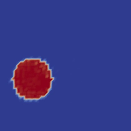
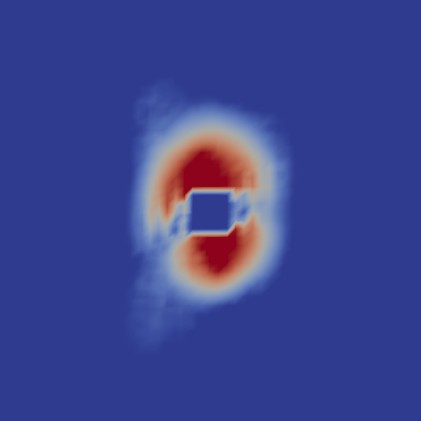
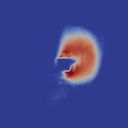
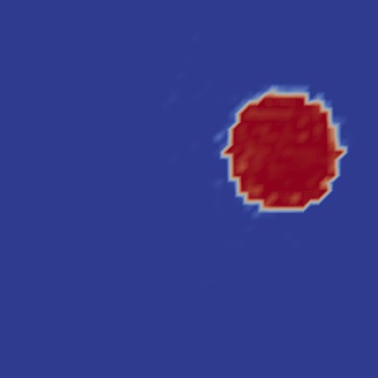
Figure 2: Density flow under constraints $|u|\leq 20$

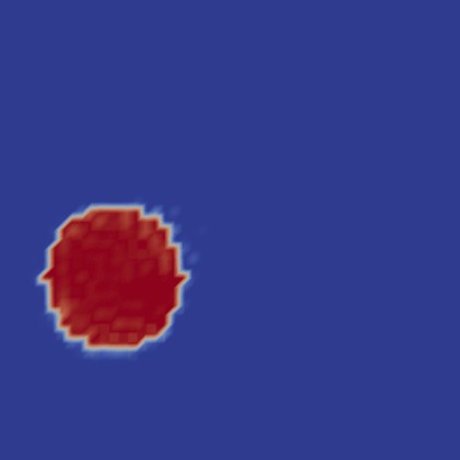
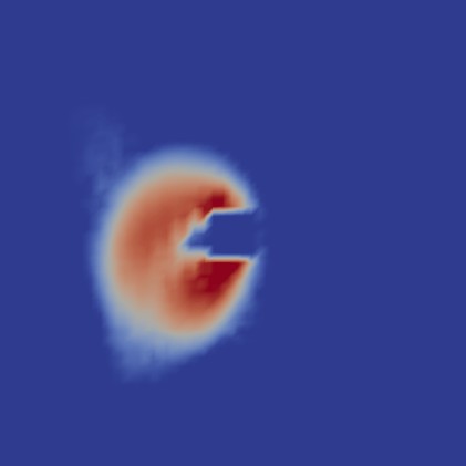
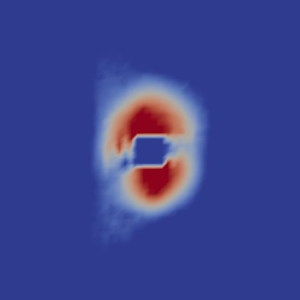
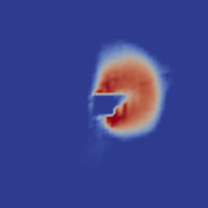
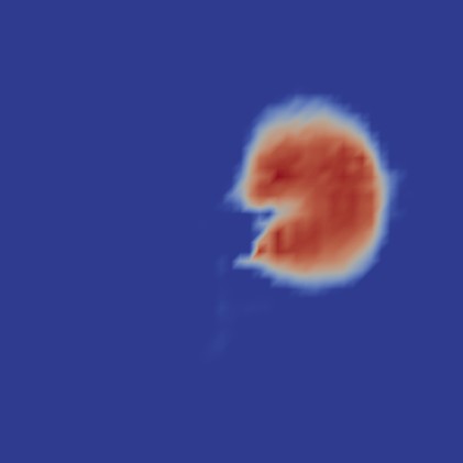
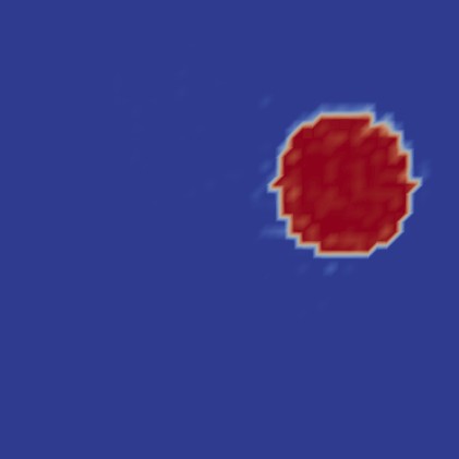
Figure 3: Density flow under constraints $|u|\leq 1$.

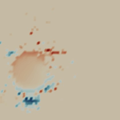
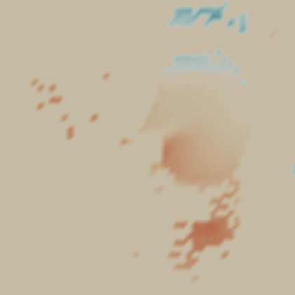
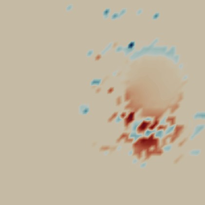
Figure 4: Input on space $|u|\leq 20$.

Figure 5: Input on space, $|u|\leq 1$.

4 Conclusion

In this paper, we have studied optimal mass transport of affine nonlinear control systems under input and density constraints. The proposed algorithms has guaranteed convergence under mild conditions. Future direction includes extending these results to systems on large scale graphs.

5 Acknowledgement

We would like to thank Professor Pontus Giselsson for insightful discussions and valuable feedback during the preparation of this manuscript.

We have used dolfinx [3] to solve the PDEs in this paper. And the computations were enabled by resources provided by the Swedish National Infrastructure for Computing (SNIC) at the PDC Center for High Performance Computing, KTH Royal Institute of Technology, partially funded by the Swedish Research Council through grant agreement no. 2018-05973.

6 Appendix

Computation of ${\rm prox}_{N}(\mu,\eta,\xi)$

By definition of the proximal operator

$${\rm prox}_{N}(\mu,\eta,\xi)$$

$$= \inf_{\tilde{\mu},\tilde{\eta},\tilde{\xi}}\int\frac{1}{2}|\tilde{\mu}-\mu|^{2}+\frac{1}{2}|\tilde{\xi}-\xi|^{2}+\frac{1}{2}|\tilde{\eta}_{0}-\eta_{0}|^{2}dxdt$$

$$\quad+\int\frac{1}{2}|\tilde{\eta}_{1}-\eta_{1}|^{2}+\frac{1}{2}|\tilde{\eta}_{2}-\eta_{2}|^{2}dx$$ (8)

under the constraints

$$\begin{cases}\nabla_{t,x}\cdot\tilde{\mu}=\tilde{\eta}_{0}\\ \tilde{\rho}(0,\cdot)=\tilde{\eta}_{1},\tilde{\rho}(T,\cdot)=\tilde{\eta}_{2}\\ R\tilde{\mu}=\tilde{\xi}\end{cases}$$

We substitute the last two constraints into (8), and then we are left with two optimization variables, namely, $\tilde{\mu}$ and $\tilde{\eta}_{0}$. Introduce a Lagrangian multiplier $\phi(t,x)$ and define $\phi_{Q}(t,x)=\phi\left(Q^{-1}\begin{bmatrix}t\\ x\end{bmatrix}\right)$ for the first constraint, where

$$Q=(I+R^{\top}R)^{-1}.$$

The problem then becomes

$$\inf_{\tilde{\mu},\tilde{\eta}_{0}}\sup_{\phi} \int\frac{1}{2}|\tilde{\mu}-\mu|^{2}+\frac{1}{2}|R\tilde{\mu}-\xi|^{2}+\frac{1}{2}|\tilde{\eta}_{0}-\eta_{0}|^{2}dxdt$$

$$+\int\frac{1}{2}|\tilde{\rho}(0,\cdot)-\eta_{1}|^{2}+\frac{1}{2}|\tilde{\rho}(T,\cdot)-\eta_{2}|^{2}dx$$

$$-\int Q^{-1}\nabla\phi\cdot\tilde{\mu}+\phi\tilde{\eta}_{0}dxdt$$

$$+\int\phi_{Q}(T,\cdot)\tilde{\rho}(T,\cdot)-\phi_{Q}(0,\cdot)\tilde{\rho}(0,\cdot)dx$$

Algorithm 3 Douglas-Rachford based Algorithm

Initialization: $(\mu^{0},\eta^{0},\xi^{0},\overline{\mu}^{0},\overline{\eta}^{0},\overline{\xi}^{0})$ given arbitrarily.

Repeat:

1. Calculate $\hat{\mu}^{k},\hat{\eta}^{k},\hat{\xi}^{k}$:

   $$\hat{\mu}^{k} =2\mu^{k}-\overline{\mu}^{k},$$

   $$\hat{\eta}^{k} =2\eta^{k}-\overline{\eta}^{k},$$

   $$\hat{\xi}^{k} =2\xi^{k}-\overline{\xi}^{k}$$

2. Calculate $\mu^{k+1},\eta^{k+1},\xi^{k+1}$:

   1. $\mu^{k+1}=\mu^{k}+\Phi(\hat{\mu}^{k})-\bar{\mu}^{k}$, where $\Phi(\hat{\mu}^{k})$ is the solution to the finite dimensional nonlinear equation (only the positive root of $\tilde{\rho}$ is relevant):

      $$\left\{\begin{aligned} &\rho-\hat{\rho}^{k}-\frac{|B^{{\dagger}}m|^{2}}{2(\hat{\rho}^{k})^{2}}+\frac{1}{2}|B^{{\dagger}}f|^{2}=0\\ &m-\hat{m}^{k}+\frac{(B^{{\dagger}})^{\top}B^{{\dagger}}m}{\rho}-(B^{{\dagger}})^{\top}B^{{\dagger}}f=0\end{aligned}\right.$$ (9)

      with dependent variables $(\rho,m)$.

   2. $\eta^{k+1}=\eta^{k}+\theta-\bar{\eta}^{k}$.

   3. Solve $\xi^{k+1}=\arg\min_{\xi\leq\gamma}\frac{1}{2}|\xi-\hat{\xi}^{k}|^{2}$ pointwisely.

3. Find $\phi^{k}$ by solving the PDE:

   $$-\Delta_{t,x}\phi^{k}+\phi^{k}=\nabla\cdot(\mu^{k+1}+R^{\top}\xi^{k+1})-\eta_{0}^{k+1}$$

   with boundary conditions:

   $$\left\{\begin{aligned} &\left.\partial_{t}\phi^{k}\right|_{t=0}-\phi^{k}(0,\cdot)=\eta_{1}^{k+1}\\ &\hskip 85.35826pt-(\mu^{k+1}+R^{\top}\xi^{k+1})_{0}(0,\cdot)\\ &\left.\partial_{t}\phi^{k}\right|_{t=T}+\phi^{k}(T,\cdot)=\eta_{2}^{k+1}\\ &\hskip 85.35826pt-(\mu^{k+1}+R^{\top}\xi^{k+1})_{0}(T,\cdot)\\ &\left.\partial_{i}\phi^{k}\right|_{x_{i}=0,1}=-(R^{\top}\xi^{k+1})_{i}|_{x_{i}=0,1},\quad\forall i\end{aligned}\right.$$ (10)

   where $\partial_{i}\phi^{k}=\partial\phi^{k}/\partial x_{i}$.

4. Update $\overline{\mu}^{k+1},\overline{\eta}^{k+1},\overline{\xi}^{k+1}$:

   $$\bar{\mu}^{k+1} =Q^{-1}(\nabla\phi^{k}+\mu^{k+1}+R^{\top}\xi^{k+1})$$

   $$\bar{\eta}_{0}^{k+1} =\phi^{k}+\eta_{0}^{k+1}$$

   $$\overline{\eta}_{1}^{k+1} =\rho^{k+1}(0,\cdot)-\phi^{k}(0,\cdot)$$

   $$\bar{\eta}_{2}^{k+1} =\rho^{k+1}(T,\cdot)+\phi^{k}(T,\cdot)$$

   $$\bar{\xi}^{k+1} =R\bar{\mu}^{k+1}$$

from which the KKT condition can be derived:

$$\tilde{\mu}-\mu+R^{\top}(R\tilde{\mu}-\xi)-Q^{-1}\nabla\phi =0$$

$$\tilde{\eta}_{0}-\eta_{0}-\phi =0$$

$$\tilde{\rho}(0,\cdot)-\eta_{1}-\phi_{Q}(0,\cdot) =0$$

$$\tilde{\rho}(T,\cdot)-\eta_{2}+\phi_{Q}(T,\cdot) =0$$

Solving $\phi$ from the KKT condition and plugging into the cost, we get

$$\sup_{\phi} \int\frac{1}{2}|b+\nabla\phi-\mu|^{2}+\frac{1}{2}|R(b+\nabla\phi)-\xi|^{2}+\frac{1}{2}\phi^{2}dxdt$$

$$+\int\frac{1}{2}\phi_{Q}(0,\cdot)^{2}+\frac{1}{2}\phi_{Q}(T,\cdot)^{2}dx$$

$$+\int-Q^{-1}\nabla\phi\cdot(b+\nabla\phi)-\phi(\eta_{0}+\phi)dxdt$$

$$+\int\phi_{Q}(T,\cdot)(\eta_{2}-\phi_{Q}(T,\cdot))-\phi_{Q}(0,\cdot)(\eta_{1}+\phi_{Q}(0,\cdot))dx$$

where $b=Q(\mu+R^{\top}\xi)$. To find the optimal $\phi$, it is sufficient to equate the variation of the cost at $\phi$ to $0$. That is, for all $\varphi$, there must hold

$$0=- \int\nabla\varphi\cdot(\mu+R^{\top}\xi+Q^{-1}\nabla\phi)-\varphi(\phi+\eta_{0})dxdt$$

$$+\int \varphi(T,\cdot)(\eta_{2}-\phi_{Q}(T,\cdot))-\varphi(0,\cdot)(\eta_{1}+\phi_{Q}(0,\cdot))dx$$

Applying integration by parts yields

$$\int\varphi\{(\nabla\cdot(\mu+R^{\top}\xi+\nabla\phi_{Q})-(\phi+\eta_{0})\}dxdt$$

$$+ \int\varphi(0,\cdot)[(\mu+R^{\top}\xi)_{0}(0,\cdot)+\partial_{t}\phi_{Q}(0,\cdot)]dx$$

$$+ \int-\varphi(T,)[(\mu+R^{\top}\xi)_{0}(T,\cdot)+\partial_{t}\phi_{Q}(T,\cdot)]dx$$

$$+ \sum_{i=1}^{n}\varphi|_{x_{i}=0}[(\mu+R^{\top}\xi)_{i}+\partial_{i}\phi_{Q})]_{x_{i}=0}$$

$$+ \sum_{i=1}^{n}\varphi|_{x_{i}=1}[(\mu+R^{\top}\xi)_{i}+\partial_{i}\phi_{Q})]_{x_{i}=1}$$

$$+ \int\varphi(T,\cdot)[\eta_{2}-\phi_{Q}(T,\cdot)]-\varphi(0,\cdot)[\eta_{1}+\phi_{Q}(0,\cdot)]dx$$

Since $\varphi$ is arbitrary, we immediately get

$$\Delta\phi_{Q}+\nabla\cdot(\mu+R^{\top}\xi)-(\phi_{Q}+\eta_{0})=0$$

$$\partial_{t}\phi_{Q}(0,\cdot)+(\mu+R^{\top}\xi)_{0}(0,\cdot)-\eta_{1}(\cdot)-\phi_{Q}(0,\cdot)=0$$

$$-\partial_{t}\phi_{Q}(T,\cdot)-(\mu+R^{\top}\xi)_{0}(T,\cdot)+\eta_{2}(\cdot)-\phi_{Q}(T,\cdot)=0$$

$$\partial_{i}\phi_{Q}|_{x_{i}=0,1}+(R^{\top}\xi)_{i}|_{x_{i}=0,1}=0$$

Once $\phi_{Q}$ has been found, we can solve for the optimal solution by employing the KKT condition.

References

- [1] Andrei Agrachev and Paul Lee. Optimal transportation under nonholonomic constraints. Transactions of the American Mathematical Society, 361(11):6019–6047, 2009.
- [2] Luigi Ambrosio and Séverine Rigot. Optimal mass transportation in the Heisenberg group. Journal of Functional Analysis, 208(2):261–301, 2004.
- [3] Igor A Barrata, Joseph P Dean, Jørgen S Dokken, Michal Habera, Jack Hale, Chris Richardson, Marie E Rognes, Matthew W Scroggs, Nathan Sime, and Garth N Wells. Dolfinx: The next generation fenics problem solving environment. 2023.
- [4] Jean-David Benamou and Yann Brenier. A computational fluid mechanics solution to the Monge-Kantorovich mass transfer problem. Numerische Mathematik, 84(3):375–393, January 2000.
- [5] Patrick Bernard and Boris Buffoni. Optimal mass transportation and mather theory. Journal of the European Mathematical Society, 9(1):85–121, 2007.
- [6] Yongxin Chen, Tryphon T Georgiou, and Michele Pavon. Optimal steering of a linear stochastic system to a final probability distribution, part i. IEEE Transactions on Automatic Control, 61(5):1158–1169, 2015.
- [7] Yongxin Chen, Tryphon T Georgiou, and Michele Pavon. Optimal transport over a linear dynamical system. IEEE Transactions on Automatic Control, 62(5):2137–2152, 2016.
- [8] Laurent Condat. A primal–dual splitting method for convex optimization involving Lipschitzian, proximable and linear composite terms. Journal of optimization theory and applications, 158(2):460–479, 2013.
- [9] Jim Douglas and Henry H Rachford. On the numerical solution of heat conduction problems in two and three space variables. Transactions of the American mathematical Society, 82(2):421–439, 1956.
- [10] Karthik Elamvazhuthi, Siting Liu, Wuchen Li, and Stanley Osher. Dynamical optimal transport of nonlinear control-affine systems. Journal of Computational Dynamics, 10(4):425–449, 2023.
- [11] Massimo Fornasier, Benedetto Piccoli, and Francesco Rossi. Mean-field sparse optimal control. Philosophical Transactions of the Royal Society A: Mathematical, Physical and Engineering Sciences, 372(2028):20130400, 2014.
- [12] Massimo Fornasier and Francesco Solombrino. Mean-field optimal control. ESAIM: Control, Optimisation and Calculus of Variations, 20(4):1123–1152, 2014.
- [13] Nassif Ghoussoub, Young-Heon Kim, and Aaron Zeff Palmer. Optimal transport with controlled dynamics and free end times. SIAM Journal on Control and Optimization, 56(5):3239–3259, 2018.
- [14] Romain Hug, Emmanuel Maitre, and Nicolas Papadakis. On the convergence of augmented lagrangian method for optimal transport between nonnegative densities. Journal of Mathematical Analysis and Applications, 485(2):123811, 2020.
- [15] Said Kerrache and Yasushi Nakauchi. Constrained mass optimal transport. arXiv preprint arXiv:2206.13352, 2022.
- [16] Vishaal Krishnan and Sonia Martínez. Distributed optimal transport for the deployment of swarms. In 2018 IEEE Conference on Decision and Control (CDC), pages 4583–4588. IEEE, 2018.
- [17] Nicolas Papadakis, Gabriel Peyré, and Edouard Oudet. Optimal transport with proximal splitting. SIAM Journal on Imaging Sciences, 7(1):212–238, 2014.
- [18] Anders Rantzer. A dual to Lyapunov’s stability theorem. Systems & Control Letters, 42(3):161–168, 2001.
- [19] Bàng Công Vũ. A splitting algorithm for dual monotone inclusions involving cocoercive operators. Advances in Computational Mathematics, 38(3):667–681, 2013.